CHAPTER 5

SINGLE-CASE EXPERIMENTAL DESIGNS

Michael Perone and Daniel E. Hursh

Single-case experimental designs are characterized by repeated measurements of an individual's behav­ior, comparisons across experimental conditions imposed on that individual, and assessment of the measurements' reliability within and across the con­ditions. Such designs were integral to the develop­ment of behavioral science. Early work in the field of psychology depended on the analysis of the expe­riences of one or a few individuals (Ebbinghaus, 1885/1913; Thorndike, 1911; Wertheimer, 1912). The investigator identified a phenomenon (e.g., learning and memory, the law of effect, the phi phe­nomenon) and pursued experimental arrangements that assessed its reliability and the functional rela­tions among the pertinent variables (e.g., the rela­tion between the length of a series of nonsense syllables and learning curves, recall, and retention; the relation between the consequences of behavior and the rate of the behavior; the relation between an observer's distance from blinking lights and appear­ance of movement). Because the research was con­ducted on the investigators themselves (e.g., the memory work of Ebbinghaus) or on just a few par­ticipants (e.g., Thorndike's cats and Wertheimer's human observers), the experimental arrangements often involved intensive study, with numerous mea­surements of behavior recorded while each individ­ual was studied under a variety of conditions.

Only after the development of statistical methods for analyzing aggregate data did the focus shift to comparisons across groups of participants, with each group exposed to a single condition (see also Chapter 8, this volume). In the original case, the

"participants" were plants in fields split into plots. The statistical methods were developed to assess the significance of differences in yields of plots of plants treated differently. R. A. Fisher's (1925) Statistical Methods for Research Workers set the course for the field. Fisher began development of his methods while employed as the statistician at an agricultural experiment station early in his career. The fact that data on large numbers of participants tend to be normally distributed (regardless of whether the par­ticipants are plants, people, or other animals) led to the easy adaptation of group statistical methods to research with humans. The standard practice came to emphasize the importance of group means, differ­ences in these means, and the use of statistical tests to draw inferences about the likelihood that the group differences were representative of differences in the populations of interest (e.g., Kazdin, 1999; Perone, 1999).

Despite the rise of group statistical methods, Single-case designs continued to be used in some important work because they allowed the investiga­tor to study the details of relations among variables as expressed in the behavior of individuals (e.g., Bijou, 1955; Skinner, 1938; Watson, 1913), which resulted in reasonably clear demonstrations of func­tional relations among the variables being studied (e.g., conditioned startle responses, reinforcement, and schedules of reinforcement). Articulation of the necessary elements of Single-case designs, notably in Sidman's (1960) seminal Tactics of Scientific Research, helped make the designs practically de rigueur in basic research on free-operant behavior

DOl: 10.1037/13937-005 APAHandbook ofBehaviorAnalysis:Vol. 1. Methods and Principles, G.]. Madden (Editor-in-Chief)

- ~ - --~ ..... ~ A ••• : l')_~ ..... 1-.,..,1 ....,.,.;,.,,1 ACcor'-:llirm All richts reserved. 107 .1

Perone andHursh

(Baron &:. Perone, 1998;]ohnston &:. Pennypacker, 2009; Perone, 1991). Translation of basic laboratory research for application in everyday situations resulted in the further development of how single­case research designs were to serve applied research­ers (Baer, Wolf, &:. Risley, 1968, 1987; Bailey &:. Burch, 2002; Barlow, Nock, &:. Hersen, 2009; Mor­gan &:. Morgan, 2009; see Chapter 8, this volume).

In this chapter, we describe and provide exam­ples of the various design elements that constitute single-case methods. We begin by considering the fundamental requirement of any experiment­internal validity-and the kinds of obstacles to internal validity that are most likely to be encoun­tered in single-case experiments. Next, we describe a variety of designs, ranging in complexity, that are commonly associated with the single-case approach. Included are designs to study irreversible or revers­ible changes in behavior, experimental conditions arranged successively or simultaneously, and the effects of one or more independent variables. In each instance, we evaluate the degree to which the design can overcome obstacles to internal validity. Some designs, for practical or ethical reasons, exclude important controls and thus compromise internal validity, but most single-case designs are robust in promoting internal validity. A great strength of the single-case approach is its flexibility, and we describe how single-case designs can be adjusted dynamically, over the course of an experi­ment, in response to the ongoing pattern of results. We go on to review the commitment of single-case investigators to identifying and taking command of the variables that control behavior. This commit­ment is expressed in the steady-state strategy that underlies most contemporary single-case research. Finally, we describe how interparticipant replication, a seeming departure from a Single-case approach, is needed to assess the degree to which an investigator has succeeded in identifying and controlling relevant variables (see also Chapter 7, this volume).

INTERNAL VALIDITY OF SINGLE-CASE EXPERIMENTS

The essential goal of an experiment is to make valid decisions about causal relations between the

variables of interest. When the results of an experi­ment provide clear evidence that manipulation of the independent variable caused the changes mea­sured in the dependent variable, the experiment is said to have internal validity. Investigators are also concerned with other kinds of validity. Kazdin (1999) and Shadish, Cook, and Campbell (2002) listed construct validity, statistical conclusion valid­ity, and external validity. Of these, external validity, which is concerned with the generality of experi­mental outcomes across populations, settings, times, or variables, seems to draw the lion's share of atten­tion from methodologists. This critically important issue is addressed by Branch and Pennypacker in this volume's Chapter 7. Here we need only say that from the standpoint of experimental design, internal validity takes precedence because it is prerequisite to external validity. Unless an investigator can describe the functional relation between the inde­pendent and dependent variables with confidence, worrying about the generality of the relation would be premature. As Campbell and Stanley (1963) put it, "Internal validity is the basic minimum without which an experiment is uninterpretable" (p. 5). (For a thoughtful discussion of the interplay between internal and external validity, see Kazdin, 1999, pp. 35-38, and for a more general discussion considering all four types of validity, see Shadish et al., 2002, pp. 93-102.)

Experimental designs are judged largely in terms of how well they promote internal validity. It may be helpful to think of a completed experiment as a kind of argument in which the design and results lead to a con­clusion about causality. Internal validity has to do with the persuasiveness of the argument. Consumers of the research-journal reviewers and editors initially-will differ in their susceptibility to the argument, which is why editors weigh the judgments of several reviewers to render a verdict on the validity of an experiment and whether a report of it merits publication.

It may also be helpful to remember, as you read this or any other chapter about experimental design, that good design can only foster internal validity; it cannot guarantee it. Internal validity is determined not only by the experimental design but also by the experimental outcomes. Consider, for example, a Simple experiment to evaluate a treatment to reduce

108

Single-Case Experimental Designs

smoking. The investigator begins by taking a few weeks to measure the baseline rate of smoking (e.g., in cigarettes per day). Suppose the treatment is' applied, and after a few weeks smoking ceases alto­gether. Finally, the treatment is withdrawn, that is, the investigator reinstates the baseline conditions. What happens next is critical to an evaluation of the experiment's internal validity. If smoking recovers, returning to levels near those observed during the initial baseline, the investigator can make a strong inference about the reductive effect of the treatment on smoking. If smoking fails to recover, however, the causal status of the treatment is ambiguous. It might have been the cause of a permanent reduction in smoking, but the evidence is open to alternative accounts. It is possible that some other variable, operating over the course of time, is responsible for the absence of smoking. Fortunately, there are ways to resolve the ambiguity; they are discussed later in the Designs for Irreversible Effects section. The gen­eral point remains: A final decision about internal validity must wait until the data have been collected and analyzed and conclusions about the effect of the experimental treatment have been made.

Internal validity is fostered by designs that elimi­nate or reduce the influence of extraneous variables that could compete with the independent variable for control of the dependent variable. The investiga­tor's design objective is to eliminate such variables­famously labeled by Campbell and Stanley (1963) as threats to internal validity-or, if that is not possible, to equalize their effects across experimental condi­tions so that they are not confounded with the inde­pendent variable. Because single-case experiments compare conditions imposed on an individual, investigators must guard against threats that operate as a function of time or repeated exposure to experi­mental treatments: history, maturation, testing, and instrumentation.

History, in this context, generally refers to the influence of factors outside the laboratory. For example, an increase in the tobacco tax during a smoking cessation study could contribute to a smoker's success in giving up the habit and inflate the apparent effect of the experimental treatment.

Maturation refers to processes occurring within the research participant. As the name implies, they

may be developmental in character; for example, with age, changes in cognitive and social develop­ment could affect the efficacy of cartoons as rein­forcers. Maturational variables may also involve shorter term processes such as fatigue, boredom, and hunger, and investigators should be aware of these processes even in highly controlled laboratory experiments. Working in the animal laboratory, McSweeney and her colleagues (e.g., McSweeney &:

Roll, 1993) showed that even when the procedure is held constant, response rates may change systemati­cally over the course of a session. There has been some disagreement about the responsible process (the primary contenders are satiation and habitua­tion; see McSweeney &: Murphy, 2000), but from the standpoint of experimental design this disagree­ment does not matter. What does matter is that any design that compares treatment conditions arranged early and late in a session may confound the condi­tions with a maturational process.

Testing is a concern when repeated exposure to a measurement procedure may, in itself, affect behav­ior. Investigators who rely on verbal measures may be especially concerned. It is obvious that asking a participant the same questions over and over could lead to stereotyped answers, thus blocking the test's sensitivity to changes in experimental treatments. It may be less obvious that purely operant procedures are also susceptible to the testing threat. For exam­ple, as rats gain experience with fixed-ratio sched­ules, they tend to acquire increasingly efficient response topographies. Over a series of sessions with a fixed-ratio schedule, these changes in responding will be confounded with the effects of the experimental conditions.

Instrumentation is a threat when systematic changes or drift in a measuring device may contami­nate the data collected over the course of a study. An investigator may neglect to periodically recalibrate the force required to activate an operandum, for example, or the sensitivity of a computer touch screen may be reduced by repeated use. The instru­mentation threat is most likely an issue in research that relies on human observers to collect or code data (Chapter 6, this volume). Prudent investigators will carefully consider both the methods used to train their human observers and those aspects of

109

Perone and Hursh

their experimental protocol that may influence the consistency of the observers' work.

These four time- and experience-related threats to internal validity can be addressed successfully in single-case designs by way of replication. Through­out an experiment, behavior is measured repeatedly so that the effect of the experimental manipulation can be assessed on a nearly continuous basis. Kazdin (1982) emphasized the importance of repeated measurement by calling it the fundamen­tal requirement of single-case designs (p, 104). If the behavioral measures show (a) minimal varia­tion in value across time within each experimental condition, (b) systematic differences across condi­tions, and (c) comparable values when conditions are replicated, then the experimental manipulation is the most plausible causal factor. With such a pat­tern of results, the influence of extraneous factors categorized as history, maturation, testing, or instrumentation would appear to be either elimi­nated or held constant.

DESIGNS

Next, we turn to some illustrative designs and con­sider the degree to which they are likely to be suc­cessful in addressing threats to internal validity.

Designs Without Replicated Conditions Two simple designs that omit replication of experi­mental conditions have appeared in the literature. These designs do, however, involve repeated mea­surement within a condition, allowing investigators to rely on patterns in the results over time to assess the possible impact of an intervention.

The intervention-only design (Moxley, 1998) is most useful in situations in which it is unethical to take the time to collect baseline data (as with dan­gerous or illegal behavior) or it is not feasible (as in instructional situations in which the yet-to-be­taught behavior is absent from the participant's rep­ertoire). The data collected early in the process of intervening serves as a kind of baseline for changes that occur as the intervention proceeds. Changes that are systematic, such as accelerations, decelera­tions, or changes in variability, are taken as evidence of the intervention's effectiveness.

llO

Considered in the abstract, the intervention-only design would appear to be unacceptably weak in its defense against threats to internal validity. Consider the idealized pattern of results in Figure 5.1. The increase in behavior could be the result of the inter­vention, but it is also easy to imagine how it might result from, say, historical or maturational factors. Details about the procedure and the independent and dependent variables might lead to a more posi­tive evaluation of the study'S validity. Suppose, for example, the behavior represented in Figure 5.1 is correct operations of a factory machine and the intervention is some procedure for training the cor­rect operation. Suppose also that the machine is unique in both form and operation-nothing similar is available outside the factory training environ­ment. Under these restricted circumstances, attrib­uting the improved performance to the training is plausible. Still, one must admit that the conclusion is limited, and the restricted circumstances needed to support it might be rare.

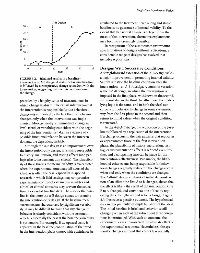
The baseline intervention or A-B deSign improves on the intervention-only design by adding a true baseline phase. In the idealized results shown in Figure 5.2, a stable behavioral baseline is followed by a conspicuous change that coincides with the intervention. The time course of behavioral change in the intervention phase is similar to that shown in Figure 5.1 for the intervention-only design. The evi­dence of an intervention effect is strengthened in the A-B design because the intervention results are

Intervention-Qnly Design 40

3S

30

C<: 25 0 ~ 20

~ 15 <Xl

10

5

0 0 5 10 15 20 25

TIME

FIGURE 5.1. Idealized results in an intervention-only design. The increase in behavior over the initial val­ues, consistent with the goal or expected effect of the intervention, is taken as evidence that the intervention caused the increase.

Single-Case Experimental Designs

A-B Design attributed to the treatment. Even a long and stable 30 B baseline is no guarantee of internal validity: To the

extent that behavioral change is delayed from the 25

onset of the intervention, alternative explanations 20

may become increasingly plausible. ex: 0

In recognition of these sometimes insurmount­

I I I I ! I IIII ! IIII I I I I

A

20 25

~ 15 :I: uJ able limitations of designs without replications, a '" 10

considerable range of designs has evolved that 5 includes replications.

0 ~: 0 5 10 15

TIME

FIGURE 5.2. Idealized results in a baseline­intervention or A-B design. A stable behavioral baseline is followed by a conspicuous change coincident with the intervention, suggesting that the intervention caused the change.

preceded by a lengthy series of measurements in which change is absent. The causal inference-that the intervention is responsible for the behavioral change-is supported by the fact that the behavior changed only when the intervention was imple­mented. More generally, an immediate change in level, trend, or variability coincident with the begin­ning of the intervention is taken as evidence of a possible functional relation between the interven­tion and the dependent variable.

Although the A-B design is an improvement over the intervention-only design, it remains susceptible to history, maturation, and testing effects (and per­

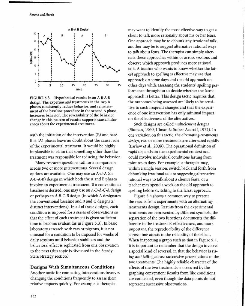
Designs With Successive Conditions A straightforward extension of the A-B design yields a major improvement in promotinginternal validity: Simply reinstate the baseline condition after the intervention-an A-E-A design. A common variation is the B-A-B design, in which the intervention is imposed in the first phase, withdrawn in the second, and reinstated in the third. In either case, the under­lying logic is the same, and in both the ideal out­come is for behavior to change in some systematic way from the first phase to the second and then return to initial values when the original condition is reinstated.

In the A-B-A-B design, the replication of the base­line is followed by a replication of the intervention. If a change occurs in the data patterns that replicates or approximates those of the first intervention phase, the plausibility of history, maturation, test­ing, or instrumentation effects is reduced even fur­ther, and a compelling case can be made for the

I:

I

haps also to instrumentation effects). The plausibil­ity of these threats to internal validity is exacerbated when the experimental outcomes fall short of the ideal, as is often the case, especially in applied research in which field settings may compromise experimental control of extraneous variables and ethical or clinical concerns may prevent the collec­tion of extended baseline data. The shorter the base­line is, the more the A-Bdesign comes to resemble the intervention-only design. If the baseline mea­surements are characterized by significant variabil­ity, it may be difficult to claim that any change in behavior is clearly coincident with the treatment, which is especially the case if the baseline variability is systematic. For example, if an upward trend is apparent in the baseline, continuation of the trend in the intervention phase cannot with confidence be

intervention's effectiveness. Put Simply, the likeli­hood of other events being responsible for behav­ioral changes is greatly reduced if the changes occur when and only when the conditions are changed. The A-B-A-B design contains an initial demonstra­tion of an effect (the first A to B change), shows that the effect is likely the result of the intervention (the B to A change), and convinces one of that by repli­cating the effect (the second A to B change). Figure 5.3 illustrates a possible outcome. The hypothetical data in this particular example fall short of the ideal: The initial baseline is brief, and behavior is still changing when each of the subsequent three condi­tions is terminated. With such an outcome, the experiment leaves unanswered the ultimate effect of the experimental treatment. Nevertheless, the sys­tematic changes in trend that coincide repeatedly

111

Perone andHUTsh

A-B-A-BDesign 30

A: B : A l B

25 V-: : : 20

a: o ~ 15 :I: UJ co 1'- Vl~I I~,10 I I l

I I I I I I I I ,5 I I I I I I I • I

5 10 15 20 25 30 35

TIME

FIGURE 5.3. Hypothetical results in an A-B-A-B design. The experimental treatments in the two B phases consistently reduce behavior, and reinstate­ment of the baseline procedure in the second A phase increases behavior. The reversibility of the behavior change in this pattern of results supports causal infer­ences about the experimental treatment.

with the initiation of the intervention (B) and base­line (A) phases leave no doubt about the causal role of the experimental treatment. It would be highly implausible to claim that something other than the treatment was responsible for reducing the behavior.

Many research questions call for a comparison across two or more interventions. Several design options are available. One may use an A-B-A (or A-B-A-B) design in which both the A and B phases involve an experimental treatment. If a conventional baseline is desired, one may use an A-B-A-C-Adesign or perhaps an A-B-C-B design (in which A designates the conventional baseline and Band C designate distinct interventions). In all of these designs, each condition is imposed for a series of observations so that the effect of each treatment is given sufficient time to become evident (as in Figure 5.3). In basic laboratory research with rats or pigeons, it is not unusual for a condition to be imposed for weeks of daily sessions until behavior stabilizes and the behavioral effect is replicated from one observation to the next (this topic is discussed in the Steady­State Strategy section).

Designs With Simultaneous Conditions Another tactic for comparing interventions involves changing the conditions frequently to assess their relative impacts quickly. For example, a therapist

112

may want to identify the most effective way to get a client to talk more rationally about his or her fears. One approach may be to debunk any irrational talk; another may be to suggest alternative rational ways to talk about fears. The therapist can simply alter­nate these approaches within or across sessions and observe which approach produces more rational talk. A teacher who wants to know whether the lat­est approach to spelling is effective may use that approach on some days and the old approach on other days while assessing the students' spelling per­formance throughout to decide whether the latest approach is better. This design tactic requires that the outcomes being assessed are likely to be sensi­tive to such frequent changes and that the experi­ence of one intervention has only minimal impact on the effectiveness of the alternatives.

Such designs are called multielement deSigns (Sidman, 1960; Ulman &: Sulzer-Azaroff, 1975). In one variation on this tactic, the alternating-treatments deSign, two or more treatments are alternated rapidly (Barlow et al., 2009). The operational definition of rapid depends on the experimental context and could involve individual conditions lasting from minutes to days. For example, a therapist may, within a Single session, switch back and forth from debunking irrational talk to suggesting alternative rational ways to talk about a client's fears, or a teacher may spend a week on the old approach to spelling before switching to the latest approach.

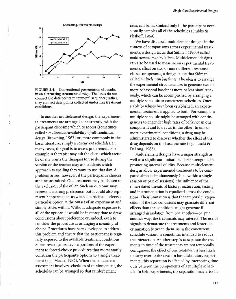
Figure 5.4 shows a common way to present the results from experiments with an alternating­treatments design. Results from the experimental treatments are represented by different symbols; the separation of the two functions documents the dif­ference in the treatments' effectiveness, and more important, the reproducibility of the difference across time attests to the reliability of the effect. When inspecting a graph such as that in Figure 5.4, it is important to remember that the design involves a special kind of reversal, in that the behavior is ris­ing and falling across successive presentations of the two treatments. The highly reliable character of the effects of the two treatments is obscured by the graphing convention: Results from like conditions are connected, even though the data points do not represent successive observations.

Single-Case Experimental Designs

Altematlng-Treatments Design

TIME

FIGURE 5.4. Conventional presentation of results in an alternating-treatments design. The lines do not connect the data points in temporal sequence; rather, they connect data points collected under like treatment conditions.

In another multielement design, the experimen­tal treatments are arranged concurrently, with the participant choosing which to access (sometimes called simultaneous-availability-of-all-conditions design [Browning, 1967] or, more commonly in the basic literature, simply a concurrent schedule). In many cases, the goal is to assess preferences. For example, a therapist may ask the client which tactic he or she wants the therapist to use during the session or the teacher may ask students which approach to spelling they want to use that day. A problem arises, however, if the participant's choices are unconstrained: One treatment may be chosen to the exclusion of the other. Such an outcome may represent a strong preference, but it could also rep­resent happenstance, as when a participant selects a particular option at the outset of an experiment and simply sticks with it. Without adequate exposure to all of the options, it would be inappropriate to draw conclusions about preference or, indeed, even to consider the procedure as arranging a meaningful choice. Procedures have been developed to address this problem and ensure that the participant is regu­larly exposed to the available treatment conditions. Some investigators devote portions of the experi­ment to forced-choice procedures that momentarily constrain the participant's options to a single treat­ment (e.g., Mazur, 1985). When the concurrent assessment involves schedules of reinforcement, the schedules can be arranged so that reinforcement

rates can be maximized only if the participant occa­sionally samples all of the schedules (Stubbs &: Pliskoff, 1969).

We have discussed multielement designs in the context of comparisons across experimental treat­ments, a design tactic that Sidman (1960) called multielement manipulations. Multielement designs can also be used to measure an experimental treat­ment's effect on two or more different response classes or operants, a design tactic that Sidman called multielement baselines. The idea is to arrange the experimental circumstances to generate two or more behavioral baselines more or less simultane­ously, which can be accomplished by arranging a multiple schedule or concurrent schedules. Once stable baselines have been established, an experi­mental treatment is applied to both. For example, a multiple schedule might be arranged with contin­gencies to engender high rates of behavior in one component and low rates in the other. In one or more experimental conditions, a drug may be administered to discover whether the effect of the drug depends on the baseline rate (e.g., Lucki &: DeLong, 1983).

Multielement designs have a major strength as well as a significant limitation. Their strength is in promoting internal validity. Because multielement designs allow experimental treatments to be com­pared almost simultaneously (i.e., within a single session or pair of sessions), the influence of the time-related threats of history, maturation, testing, and instrumentation is equalized across the condi­tions. Their limitation is that the temporal juxtapo­sition of the two conditions may generate different effects than the conditions might generate if arranged in isolation from one another-or, put another way, the treatments may interact. The use of signals to demarcate the treatments and foster dis­crimination between them, as in the concurrent schedule variant, is sometimes intended to reduce the interaction. Another step is to separate the treat­ments in time; if the treatments are not temporally contiguous, the effect of one treatment is less likely to carry over to the next. In basic laboratory experi­ments, this separation is effected by interposing time outs between the components of a multiple sched­ule. In field experiments, the separation may arise in

113

Perone andHursh

the customary scheme of things-for example, when treatments are alternated across school days or across weekly therapy sessions. There is no guaran­tee, however, that these steps actually do prevent interacting treatments. The only sure way to allay this concern is to conduct additional research in which each treatment is studied in isolation.

Designs for Irreversible Effects So far, we have considered two general classes of experimental designs. The first consists of the intervention-only and baseline-intervention (A-B) designs. Although these designs may be justifiable under special circumstances, they are undesirable because, in general, they provide little protection against time- and experience-related threats to internal validity. The second class of experimental designs promotes internal validity through replica­tion of experimental conditions. The difference between the two classes can be summarized this way: In an experiment with an A-B design, any change observed from A to B might be related to the experimental treatment, but-depending on the particulars of the experiment-the change might reflect the operation of maturation, history, testing, or instrumentation. Adding replications (e.g., in A-B-A, A-B-A-B, or multielement designs) tests these alternative explanations. Each replica­tion, if accompanied by appropriate changes in behavior, makes it less plausible that something other than the experimental treatment could have caused the changes.

To promote internal validity, the designs in the second class require that the participant experience another treatment or a return to baseline. Replicat­ing conditions is not always possible or desirable, however, for several reasons. First, some treatment effects are not likely to disappear simply because the treatment has been discontinued (e.g., the learning of a math fact, reading skill, or social skill that allows the learner access to desirable items or activi­ties). The use of an A-B-A design to assess such an irreversible outcome will yield ambiguous results: When the baseline condition is replicated, the behavior remains unchanged. It is not possible to say whether the outcome is the persistent effect of the treatment or the effect of some other factor.

114

Another problem arises in cases in which a partici­pant's experience with one treatment has an impact on the effects produced by another treatment (e.g., being taught decoding skills can result in more rapid sight word learning). If the two treatments were compared in an alternating-treatments design, their effects would be obscured. The last problem is ethi­cal rather than logistical: If the treatment effect is beneficial (e.g., reduction in self-injurious behav­ior), it would be undesirable to withdraw it and return behavior to pretreatment values even if the withdrawal might decisively demonstrate the treat­ment's efficacy.

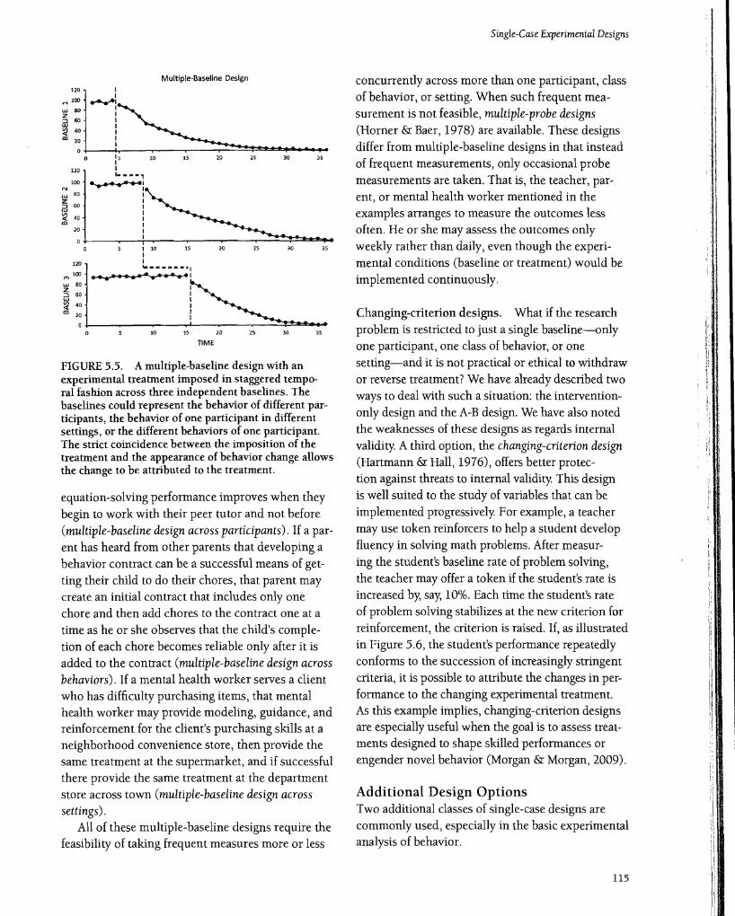
Multiple-baseline designs. One way to avoid the practical, ethical, and confounding problems of Withdrawing, reversing, or alternating treatments is to arrange for the replication of a treatment's impact to occur across participants, behaviors, or settings. These multiple-baseline designs (Baer et al., 1968) were developed just for such situations. Data are collected under two or more independent baseline conditions. The baselines often come from more than one participant, but they may also come from the same participant engaged in different behaviors or from the same participant behaving in different settings. Once the baseline behavior is shown to be stable, the experimental treatment is implemented in time-staggered fashion to one baseline (i.e., one participant, behavior, or setting) at a time. Adding the treatment to a second baseline is only done once the impact of the treatment for the first base­line has become obvious. Thus, the baseline data for untreated participants, responses, or settings serves as a control for confounding variables. That is, if changes are observed when and only when the treatment is applied to each of the participants, responses, or settings, it is unlikely that other vari­ables can account for the changes. An idealized pat­tern of results is shown in Figure 5.5.

Some examples may help illustrate the three common variants of the multiple-baseline design. If a teacher has experience suggesting that peer tutor­ing may help some of her students who struggle with solving equations, that teacher may assign a peer tutor to one struggling student at a time to observe whether each of the struggling students'

Multiple-Baseline Design

.-.'00120 I :.........1

Z 1UJ80 l~:::J 60 I

~ 40 :

! •,• al ': • f •• « ••

o : 5 10 15 20 25 30 35

1120 I•••• ,

N 100 :

LU 80 I Z 1

1 1

::J 60 1

~ 40 : al

20 1

3S

.. 10 lS 20 2S 3S'0

TIME

FIGURE 5.5. A multiple-baseline design with an experimental treatment imposed in staggered tempo­ral fashion across three independent baselines. The baselines could represent the behavior of different par­ticipants, the behavior of one participant in different settings, or the different behaviors of one participant. The strict coincidence between the imposition of the treatment and the appearance of behavior change allows the change to be attributed to the treatment.

equation-solving performance improves when they begin to work with their peer tutor and not before (multiple-baseline design across participants). If a par­ent has heard from other parents that developing a behavior contract can be a successful means of get­ting their child to do their chores, that parent may create an initial contract that includes only one chore and then add chores to the contract one at a time as he or she observes that the child's comple­tion of each chore becomes reliable only after it is added to the contract (multiple-baseline design across behaviors). If a mental health worker serves a client who has difficulty purchasing items, that mental health worker may provide modeling, guidance, and reinforcement for the client's purchasing skills at a neighborhood convenience store, then provide the same treatment at the supermarket, and if successful there provide the same treatment at the department store across town (multiple-baseline design across settings).

All of these multiple-baseline designs require the feasibility of taking frequent measures more or less

Single-Case Experimental Designs

concurrently across more than one participant, class of behavior, or setting. When such frequent mea­surement is not feasible, multiple-probe designs (Horner &: Baer, 1978) are available. These designs differ from multiple-baseline designs in that instead of frequent measurements, only occasional probe measurements are taken. That is, the teacher, par­ent, or mental health worker mentioned in the examples arranges to measure the outcomes less often. He or she may assess the outcomes only weekly rather than daily, even though the experi­mental conditions (baseline or treatment) would be implemented continuously.

Changing-criterion designs. What if the research I,

problem is restricted to just a single baseline-only I

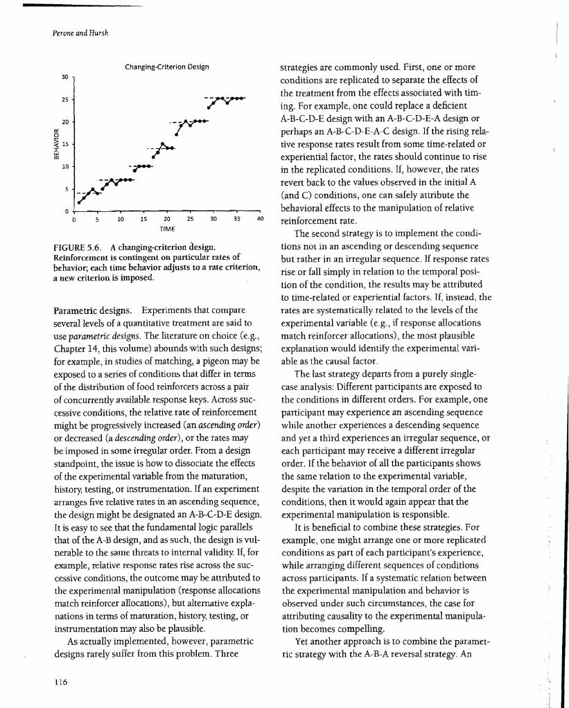
one participant, one class of behavior, or one l setting-and it is not practical or ethical to withdraw Ii or reverse treatment? We have already described two ways to deal with such a situation: the intervention­only design and the A-B design. We have also noted the weaknesses of these designs as regards internal validity. A third option, the changing-criterion design (Hartmann &: Hall, 1976), offers better protec­tion against threats to internal validity. This design is well suited to the study of variables that can be implemented progressively. For example, a teacher may use token reinforcers to help a student develop fluency in solving math problems. After measur­ing the student's baseline rate of problem solving, the teacher may offer a token if the student's rate is increased by, say, 10%. Each time the student's rate of problem solving stabilizes at the new criterion for reinforcement, the criterion is raised. If, as illustrated

'Ii'Iin Figure 5.6, the student's performance repeatedly conforms to the succession of increasingly stringent Ii,I criteria, it is possible to attribute the changes in per­

If

formance to the changing experimental treatment. II 1·1 "1As this example implies, changing-criterion designs !)

are especially useful when the goal is to assess treat­ O'if

ments designed to shape skilled performances or engender novel behavior (Morgan &: Morgan, 2009).

Additional Design Options Two additional classes of single-case designs are commonly used, especially in the basic experimental analysis of behavior.

115

Perone andHursh

Changing-Criterion Design 30

25 .rr: 20

a: .rr:o ~ 15 I UJ -r'"

10 -~

.~

5~

04--......--r---.--..---......--r--.----. o 5 10 15 20 25 30 35 40

TIME

FIGURE 5.6. A changing-criteriondesign. Reinforcement is contingent on particular rates of behavior; each time behavior adjusts to a rate criterion, a new criterion is imposed.

Parametric designs. Experiments that compare several levels of a quantitative treatment are said to use parametric designs. The literature on choice (e.g., Chapter 14, this volume) abounds with such designs; for example, in studies of matching, a pigeon may be exposed to a series of conditions that differ in terms of the distribution of food reinforcers across a pair of concurrently available response keys. Across suc­cessive conditions, the relative rate of reinforcement might be progressively increased (an ascending order) or decreased (a descending order), or the rates may be imposed in some irregular order. From a design standpoint, the issue is how to dissociate the effects of the experimental variable from the maturation, history, testing, or instrumentation. If an experiment arranges five relative rates in an ascending sequence, the design might be designated an A-B-C-D-E design. It is easy to see that the fundamental logic parallels that of the A-B design, and as such, the design is vul­nerable to the same threats to internal validity If, for example, relative response rates rise across the suc­cessive conditions, the outcome may be attributed to the experimental manipulation (response allocations match reinforcer allocations), but alternative expla­nations in terms of maturation, history, testing, or instrumentation may also be plausible.

As actually implemented, however, parametric designs rarely suffer from this problem. Three

116

strategies are commonly used. First, one or more conditions are replicated to separate the effects of the treatment from the effects associated with tim­ing. For example, one could replace a deficient A-B-C-D-E design with an A-B-C-D-E-Adesign or perhaps an A-B-C-D-E-A-C design. If the rising rela­tive response rates result from some time-related or experiential factor, the rates should continue to rise in the replicated conditions. If, however, the rates revert back to the values observed in the initial A (and C) conditions, one can safely attribute the behavioral effects to the manipulation of relative reinforcement rate.

The second strategy is to implement the condi­tions not in an ascending or descending sequence but rather in an irregular sequence. If response rates rise or fall simply in relation to the temporal posi­tion of the condition, the results may be attributed to time-related or experiential factors. If, instead, the rates are systematically related to the levels of the experimental variable (e.g., if response allocations match reinforcer allocations), the most plausible explanation would identify the experimental vari­able as the causal factor.

The last strategy departs from a purely single­case analysis: Different participants are exposed to the conditions in different orders. For example, one participant may experience an ascending sequence while another experiences a descending sequence and yet a third experiences an irregular sequence, or each participant may receive a different irregular order. If the behavior of all the participants shows the same relation to the experimental variable, despite the variation in the temporal order of the conditions, then it would again appear that the experimental manipulation is responsible.

It is beneficial to combine these strategies. For example, one might arrange one or more replicated conditions as part of each participant's experience, while arranging different sequences of conditions across participants. If a systematic relation between the experimental manipulation and behavior is observed under such circumstances, the case for attributing causality to the experimental manipula­tion becomes compelling.

Yet another approach is to combine the paramet­ric strategy with the A-B-A reversal strategy. An

Single-Case Experimental Designs

investigator might begin the experiment with a base­line Condition A (or treat the first level of the quan­titative independent variable as a baseline) and, after stabilizing behavior at each successive level of the quantitative variable (Conditions B, C, etc.), return to the baseline condition. Thus, an A-B-C-D-E design could be replaced with an A-B-A-C-A-D-A­E-A design. The obvious disadvantage is the large investment of time in repeating the baseline condi­tion. The advantage is that the effect of each treat­ment can be evaluated relative to a fixed baseline.

Factorial designs. Behavior is controlled by multi­ple variables at any given moment, and experiments may be designed to analyze such control by includ­ing all possible combinations of the levels of two or more independent variables. These factorial designs are ubiquitous in the behavioral and biomedical sci­ences. They tend to be associated with group statisti­cal traditions-indeed, a staple of graduate training in psychology is to teach the statistical methods of analysis of variance in the context of factorial research designs (e.g., Keppel &: Wickens, 2004). Nevertheless, the factorial strategy is by no means restricted to group statistical approaches (Smith, Best, Cylke, &: Stubbs, 2000) and is readily used in single-case experiments.

As an example, consider an unpublished experi­ment (Wade-Galuska, Galuska, &: Perone, 2004) concerned with variables that affect pausing on fixed-ratio schedules. A pigeon was trained on a multiple-baseline schedule in which 100 pecks on a response key produced either 2-second or 6-second access to mixed grain. Different key colors signaled the two schedule components, designated here as lean (ending in 2-second access to grain) and rich (ending in 6-second access). This arrangement (details are available in Perone &: Courtney, 1992) made it possible to study, on a within-session basis, the effects of two factors on the pausing that took place between components: the magnitude of the reinforcer delivered before the pause (the past rein­forcer, lean or rich) and the signaled magnitude of the reinforcer to be delivered on completing the next ratio (the upcoming reinforcer, lean or rich). Another factor was manipulated across successive phases of the experiment: The pigeon's body weight

was 70%, 80%, or 90% of its free-feeding weight. Thus, the experiment had a 2 X 2 X 3 factorial design (two levels of past reinforcer X two levels of upcoming reinforcer X three levels of body weight) and, therefore, 12 combinations of the levels of the three factors.

The results are shown in Figure 5.7. Each panel represents one of the body weight conditions. Note that this factor was manipulated quantitatively in an ascending series (70%,80%,90%), with a final phase devoted to a replication of the 70% condition. In this way, following the recommendations offered earlier in the Parametric Designs section, the experi­ment disentangled any confound between time- or experience-related processes and the experimental variable of body weight. Within each panel are the median pauses, calculated over the last 10 sessions of each body weight condition, in each of the four possible combinations of the other two experimental variables, the past and upcoming reinforcer magni­tudes. The past reinforcer is shown on the x-axis and the upcoming reinforcer is shown with filled (lean) and unfilled (rich) data points.

300..,------,-------,----,----..,

70 80 90 70

200

~ w (JJ

~ a.. 100

o

L R L R L R L R

PAST SCHEDULE (LEAN OR RICH)

FIGURE 5.7. A factorial design to study three factors that could affect pausing on a fixed-ratio schedule: Past schedule condition (lean [L] or rich [R], represented on the x-axis), upcoming (Upc.) schedule condition (L or R, represented by filled and unfilled circles, respectively), and body weight (expressed as a percent­age of free-feeding weight; each weight condition is represented in a different panel). Note the replication of the 70% body weight condition (rightmost panel). The results are from a single pigeon; shown are medians and interquartile ranges of the last 10 sessions of each con­dition. Data from Wade-Galuska, Galuska, and Perone (2004).

118

Perone andHursh

Within each condition, pausing was a joint func­tion of the past and upcoming schedules of rein­forcement. When the key color signaled that the upcoming schedule would be rich (unfilled circles), the past reinforcer had no apparent effect: Pausing was brief after both lean and rich schedules. When the key color signaled that the upcoming schedule would be lean (filled circles), however, the past rein­forcer had a major impact: Pausing was extended after a rich schedule. In other words, the effect of the past reinforcer was bounded by, or depended on, the signaled magnitude of the next reinforcer. When the effect of one factor depends on the level of another factor, the factors are said to interact. In the conventional terminology of factorial research design, the interaction between the past and upcom­ing magnitudes of reinforcement would be called a two-way interaction.

The interaction itself depended on the level of the body weight factor: As body weight was increased, the interaction between the past and upcoming magnitudes of reinforcement was enhanced. This kind of finding constitutes a three­way interaction. Note also that in the final phase of the experiment, replicating the 70% body weight condition reduced the interaction between the mag­nitudes to the values observed in the first phase.

In applied research, the use of single-case facto­rial designs can also prove beneficial. An example is assessment of the interaction between the type of directive and reinforcement contingencies as they affect participants' compliance with the directives and disruptive behavior (Richman et al., 2001). This three-experiment sequence first established the effectiveness of various forms of directives, then assessed their effectiveness across situations, and finally assessed the interaction between the forms of the directives and targets of differential reinforce­ment contingencies. All of the experiments used multielement designs to determine the impact of the independent variables on the outcomes for each of the participants.

Factorial designs are prevalent in the behavioral sciences specifically because they provide a frame­work for describing how multiple variables interact to control behavior. The presence of an interaction sheds light on the boundaries of a variable's effect

and thereby allows for more complete and general descriptions of functional relations between envi­ronment and behavior.

FLEXIBILITY OF IMPLEMENTATION

A strength of single-case research designs lies in the dynamics of their implementation. The examples we have offered of various Single-case designs are merely the usual ways in which the single-case research design strategy is used. It is important to recognize that, in practice, the designs may be modified in response to the pattern of results that emerges as the data are collected. Indeed, this fea­ture of the approach is what led Skinner (1956) to favor single-case designs. It is also possible to com­bine aspects of the basic single-case designs and even include aspects of group comparisons. This kind of flexibility can be an asset to any program of experimental research. It takes on special signifi­cance when the research topic is novel, when the investigator's ability to exert experimental control is limited by ethical or logistical considerations, and when the goal is to produce an empirically validated therapeutic result for an individual.

It is possible that once a behavior is changed, withdrawal of the treatment or reversal of the con­tingencies in an A-B-A design may not return the behavior to baseline values. From a therapeutic or educational standpoint, this is not a bad thing: In the long run, the therapist or teacher usually wants the participant's behavior to come under the control of, and be maintained by, the consequences it au to­matically produces, so that the participant no longer depends on an intervention or treatment (see Chap­ter 7, this volume). However, from an experimental standpoint, it is a serious problem because it leaves unanswered the question of what caused the behav­ior to change in the first place: Was it the experi­mental treatment or some process of maturation, history, testing, or instrumentation? When behavior fails to revert to baseline values in an A-B-A design, the investigator may switch to a multiple-baseline design (if data have been collected for more than one participant, behavior, or setting). Thus, it is advisable for any investigator to consider the feasi­bility of establishing multiple baselines from the

beginning, in case the behavior of interest does not return to the baseline value.

Multiple-baseline designs have their own set of challenges requiring dynamic decision making by the investigator. Sometimes imposing the experi­mental treatment on one baseline will be followed by behavioral change not only in the treated baseline but also in the as-yet-untreated baselines. This might reflect the operation of maturation, history, testing, or instrumentation-in other words, it might mean that the treatment is ineffective. Another possibility is that the treatment really is responsible for change, and the effect has spread across the baselines because they are not indepen­dent of one another. This threat to internal validity, which Cook and Campbell (1979) called diffusion of treatments, can jeopardize multiple-baseline experi­ments under several circumstances: (a) In a multiple­baseline across-participants design, all of the participants are in the same environment and may learn by observing the treatment being applied; (b) in a multiple-baseline across-behaviors design, all of the responses are coming from the same par­ticipant, and learning one response may facilitate the learning of other responses; or (c) in a multiple­baseline across-settings design, the same participant is responding in all of the settings, and when the response is treated and changed in one setting, it may change in the untreated settings. The antidote, of course, is for the investigator to select partici­pants, behaviors, or settings that experience and logic suggest will be independent of one another. Because experience and logic do not guarantee that an investigator will choose independent partici­pants, behaviors, or settings, it is advisable to select as many baselines as is feasible so that the probabil­ity of at least some of them being independent is increased.

Interdependence of a few baselines (changes occurring concurrently across those baselines) with independence of other baselines (changes occurring only when treatment is applied) in a multiple­baseline design can be informative. The investigator has the opportunity to inspect the similarities across the baselines that change concurrently and the dif­ferences between those baselines and the baselines that change only when the treatment is applied.

Single-Case Experimental Designs

These comparisons and contrasts can help to isolate the participant, behavior, and setting variables that interact with the treatment to produce the changes. For example, a teacher modeling tactics for solving various types of math problems may see students solving problems for which the solutions have yet to be modeled. If the teacher is also collecting data on the students' solving of social studies problems and does not observe those problems being solved until the solutions are modeled, one can make the case for the general effects of modeling problem solu­tions. This then sets the occasion for designing another investigation to systematically study the fea­tures of the modeling of the math problem solutions to determine which features are essential for which types of problems.

If having many baselines is not feasible and the investigator faces interdependence of all of the base­lines, the possible design tactics include (a) withdraw­ing the treatment or reversing the contingencies or (b) arranging for a changing criterion within the treatment. The first choice depends on the probabil­ity of the behavior's return to baseline values and the ethical appropriateness of such a tactic. The sec­ond choice depends on the feasibility of incorporat­ing the changing criterion into the treatment and the sensitivity of the behavior being measured to such changes. Either tactic, when successful, demon­strates the functional relation between the treatment and the outcomes. They both also set up the ratio­nale for studying the interdependence of the base­lines in a subsequent investigation. As with all efforts to investigate natural phenomena, unex­pected results help to hone understanding of the phenomena and guide further investigations.

Other design combinations may be considered. Withdrawing the treatment or reversing the contin­gencies in a successful multiple-baseline experiment can probe for the durability of the treatment effects and add another degree of replication should the changes not be durable. Gradually removing compo­nents of interventions to assess the importance of each or the intervention's durability is another varia­tion (a partialwithdrawal deSign; Rusch &:. Kazdin, 1981). Withdrawing treatment from some partici­pants, responses, or settings (a sequential with­drawal deSign; Rusch &:. Kazdin, 1981) to assess the

119

120

4

Perone andHursh

durability of treatment effects is another variation to be considered depending on the focus of the investigation.

The point of all of these additional design options is that although the research question drives the initial selection of the elements of single-case design, once the data collection begins decisions about the next condition are driven by the patterns emerging in the data being collected. Unexpected patterns can and should lead the investigator to ask how best to arrange the next phase of the investiga­tion to ensure that the original or revised research question can be answered unambiguously.

STEADY-STATE STRATEGY

Behavioral experiments assess the effect of a treat­ment by comparing behavior measured during expo­sure to the treatment with behavior measured without the treatment or, if the experimental logic dictates, with behavior measured during exposure to some other treatment. In a Single-case experiment, the conditions are imposed on an individual over some period of time, and behavior is measured repeatedly within each condition. Inferences about the experimental treatment's effectiveness are usu­ally supported by demonstrations that the difference in behavior observed across the conditions clearly exceeds any variability observed within the condi­tions. The basic strategy is not unlike the one that underlies conventional tests of statistical inference: The F ratio associated with the analysis of variance is formed by dividing an estimate of variance between experimental groups by an estimate of vari­ance within the groups, and only if the between­groups variance is large relative to the within-group variance does the investigator conclude that the experimental treatment made a statistically signifi­cant difference.

The prevailing approach in single-case experiments-the steady-state strategy-is to impose a condition until behavior is more or less stable from one measurement (session, lesson, etc.) to the next. The idea is to fix the environ­mental variables controlling behavior until the environment-behavior relation reaches equilib­rium or, as Sidman (1960) put it, a steady state.

At this point, the experimental environment is rearranged to impose the next condition, again until behavior stabilizes.

Strategic Requirements The steady-state strategy has three requirements (Perone, 1994):

1. The investigator must have sufficient control over extraneous variables to allow behavior to stabilize.

2. The investigator must be able to maintain each condition long enough to allow behavior to stabi­lize; even under ideal laboratory controls, it will take time for behavior to reach a new equilib­rium when conditions are changed.

3. The investigator must be able to recognize the steady state when it is achieved.

Meeting the first two requirements is not a mat­ter of experimental design; rather, the key issues are scientific understanding and resources, including time and access to participants' behavior. The inves­tigator must have a reasonable idea of the extrane- ' ous variables to be eliminated or held constant to allow the potential effect of the experimental vari­able to become manifest. The investigator must have the wherewithal to control the extraneous variables, and he or she must have relatively unimpeded access to the behavior of interest: An A-B-A-B design, for example, may require scores of sessions distributed over several months or more if behavior is to be given time to stabilize in each phase.

In any given area of study, initial investigations will suffer from gaps in the understanding of the behavioral processes at work and, consequently, of the variables in need of control. Persistent efforts at experimental analysis will pay dividends in identify­ing the relevant variables and developing the means to control them.

Persistence alone, however, cannot provide an investigator the access to behavior that may be needed to execute the steady-state strategy. Much depends on the nature of the topic at hand and the available resources. Investigators of topics in basic research may be in the most advantageous position, especially if they study animals. Not only are they able to control almost every facet of the animal's

living arrangements (e.g., diet, housing, light-dark cycles, opportunities to engage conspecifics), they also have unfettered access to the animal's behavior. Sessions may be conducted daily for months without interruption. Such circumstances are ideal for steady-state research.

Special problems arise when human participants replace rats and pigeons (Baron &: Perone, 1998). The typical human participant lives, works, plays, eats, drinks, and sleeps outside of the investigator's influence and is thus exposed to numerous factors that may playa role in the participant's experimental behavior (only in rare cases do human participants live in the laboratory; for an interesting example, see Bernstein &: Ebbesen, 1978). These limitations indi­cate a need for strong countermeasures, such as experimental manipulations that are "especially forcing" (Morse &: Kelleher, 1977; see also Baron &:

Perone, 1998, pp. 68-69) and increased exposure to the laboratory environment over an extended series of sessions. Unfortunately, human research-when extended access to the participant's behavior may be needed most-is when such access is most difficult to attain. Monetary incentives can help bring partici­pants to the laboratory for repeated study, of course, but even well-funded investigators will find that the number of sessions that, say, a college student will tolerate is lower than that commonly conducted in research with rats. To address this practical con­straint, some investigators arrange brief sessions, sometimes lasting as little as 10 minutes (e.g., Okouchi, 2009), and schedule a series of such ses­sions each time the participant visits the laboratory. Of course, the duration of the sessions is not the critical issue; rather, the question is whether one can complete an experiment in a few hours in the human laboratory and compare the results to experi­ments that take months or years in the animal labo­ratory. The answer will depend on the goals of the research as well as the investigator's judgment about the size of the anticipated effects and the speed of their onset. Relatively brief experiments can be defended when they are successful in producing sta­ble and reproducible behavioral outcomes within and across participants. Caution is warranted in planning and interpreting such experiments, however, because the behavioral effects of the experimental

Single-Case Experimental Designs

manipulations may not always develop according to the investigator's timetable. Sometimes there is no substitute for prolonged exposure to the contingen­cies, and what happens in the short term may not predict what happens in the long term (for an illus­tration, see Baron &: Perone, 1998, pp. 50-52). In applied research, logistical and ethical issues mag­nify the problem of behavioral access. Participants with clinically relevant repertoires may not be avail­able in large numbers, and the nature of their prob­lem behavior may sharply limit the duration of sessions. If the research is conducted in a therapeu­tic context, addressing the participant's problem will take priority over purely scientific considerations, and ethical concerns about leaving problem behav­ior untreated may restrict the nature of the experi­mental designs as well as the durations of both baseline and treatment conditions.

The steady-state strategy works best when behav­ior is measured repeatedly under controlled experi­mental conditions imposed long enough for the behavior to reach demonstrable states of equilib­rium. The pages of the]oumal of theExperimental Analysis of Behavior and the]oumal ofApplied Behavior Analysis attest that these challenges can be met. It is inevitable, however, that some experi­ments will fall short. In some cases, conducting single-case experiments in the absence of steady states will still be possible, as suggested by the hypo­thetical outcomes depicted in Figures 5.2, 5.3, and 5.6. Even in these examples, however, the number of behavioral observations is large. We suggest, therefore, that although single-case experiments may be viable in some cases without steady states, they are not likely to succeed without significant access to the behavior in the form of extensive repeated measurement (for a comprehensive discus­sion of this issue in the context of applied research, see Barlow et al., 2009, pp. 62-65 and 88-94, and Johnston &: Pennypacker, 2009, pp. 191-218).

When the efforts to achieve steady states fallshort, an investigator may consider the use of statistical tests to discriminate treatment effects from a noisy back­ground of behavioral variability. Many arguments, both pro and con, have been made in this connection (e.g., Ator, 1999; Baron, 1999; Branch, 1999; Crosbie, 1999; Davison, 1999; Kratochwill &: Levin, 2010;

121

Perone andHursh

Perone, 1999; Shull, 1999; Smith et al., 2000; Todman &: Dugard, 2001; see Chapters 7 and 11, this volume). We are concerned that reliance on inferential statistics may retard the search for effective forms of control. By comparison, the major advantage of the steady­state strategy is that it fosters the development of strong control. Unsystematic variability (noise or bounce in the data) is addressed by reducing the influence of extraneous factors and increasing the influence of the independent variable. Systematic vari­ability (the trend that occurs in the transition between steady states) is addressed by holding the experimen­tal environment constant until behavior stabilizes. Put Simply, the steady-state strategy demands that treat­ment effects be clarified by improving direct control

of behavior.

Stability Criteria The final requirement of the steady-state strategy is that of recognizing the production of a steady state. Various decision rules have been devised for this purpose. These stability criteria are often expressed in mathematical terms and indicate, in one way or another, the kind and amount of variation in behav­ior that will be acceptable over a series of observa­tions. Commonly used criteria specify (a) the number of sessions or observations to be considered in assessing the evidence of a steady state, (b) that an increasing or decreasing trend must be absent, and (c) how much bounce can be tolerated in the behavior across sessions. If the most recent behavior within a condition (e.g., responding in the last six sessions) is absent of trend and reasonably free from bounce, behavior is said to be stable.

Sidman (1960) provided the seminal discussion

of stability criteria. Detailed descriptions of stability criteria, with examples from the human and animal literature, can be found in Baron and Perone (1998) and Perone (1991).

Perhaps the most important difference among stability criteria is in how they specify the tolerable limits on bounce. Some criteria use relative mea­sures; for example, when considering the most recent six sessions, the mean response rate in the first three sessions and the mean in the last three sessions may differ by no more than 10% of the overall six-session mean. Other criteria may use

absolute measures; for example, the mean rates in the first three sessions and last three sessions may differ by no more than five responses per minute.

Not all stability criteria are expressed in quantita­tive terms. In some experiments, steady states are identified by visual inspection of graphed results. In other experiments, each condition is imposed for a fixed number of sessions (e.g., 30), and behavior in the last several sessions (e.g., five) is considered rep­resentative of the steady state.

As Sidman (1960) noted, the selection of a stabil­

ity criterion depends on the nature of the experi­mental question and the investigator'S judgment and experience. The visual stability criterion may be jus­tified, for example, when the investigator's experi­ence leads to the expectation of large or dramatic changes across conditions. The fixed-time stability criterion works well when a program of research has progressed to the point at which the investigator can confidently predict how many sessions will be needed to achieve a steady state. Even the quantita­tive criteria-the relative stability criterion and the absolute stability criterion-are specified in light of the experimental question and the investigator's judgment and experience. In the abstract, divorced from such considerations, it is impossible to say, for example, whether a 10% relative criterion is more or less stringent than a five-responses-per-minute abso­lute criterion (for a detailed discussion of the rela­tionship between relative and absolute stability criteria, see Perone, 1991, pp. 141-144).

The adequacy of a stability criterion is assessed over the course of an experiment. A criterion is ade­quate, according to Sidman (1960, p. 259), if it yields orderly and replicable functional relations between the independent and dependent variables. In this connection, it is important to recognize that any stability criterion, no matter how stringent, may be met by chance, that is, in the absence of an actual steady state. However, a criterion is highly unlikely to be repeatedly met by chance across the various experimental conditions.

ONCE IS NOT ENOUGH

Single-case designs are Single because the primary unit of analysis is the behavior of the individual

organism. Treatment effects are assessed by compar­ing the individual's response with different levels of the independent variable, and control is demon­strated by two kinds of replication: (a) the stability of the individual's behavior from one observation to the next under constant circumstances within a con­dition and (b) the stability of the change in the indi­vidual's behavior from one experimental condition to another.

The singledescriptor is misleading in that single­case research rarely involves just one individual. In addition to the within-participant forms of repli­cation that we have emphasized throughout this chapter, procedures are also replicated across participants. Single-case investigators approach interparticipant replication in two general ways, described by Sidman (1960) as direct replication and systematic replication (see also Chapter 7, this volume).

In the context of interparticipant replication, direct replication consists of repeating the experi­mental procedures with additional participants. A review of any representative sample of the literature of basic or applied behavior analysis will document that direct interparticipant replication is, for all intents and purposes, required to establish the credi­bility of single-case experimentation-even in basic laboratory research with animals, where control is at its utmost. Why, in a science devoted to the analysis of behavior in the individual organism, should be this so? Interparticipant replication is needed to show that the investigator has been successful in identifying the relevant variables and bringing them under satisfactory degrees of control. Whenever manipulation of an independent variable produces the same kind of behavioral change in a new partici­pant, one grows increasingly confident that the investigator is both manipulating the causal factor and eliminating (or otherwise controlling) the influ­ence of extraneous factors that could obscure the causal relation.

What if the attempt at interparticipant replica­tion fails? Suppose, for example, that an A-B-A-B design produces a clear, reliable effect in one partici­pant but not in another? One might be inclined to question the reality of the original result, to declare it a fluke. However, this would be a strategic error of

Single-Case Experimental Designs

elephantine proportions. A result that can be repli­cated on an intraparticipant basis (i.e., from A to B, back to A, and back again to B) cannot be dismissed so easily. The failure to replicate the effect in another participant does not negate the original finding; rather, it unveils the incompleteness of one's understanding of the original finding. The investigator may have erred in his or her operational definition of the independent variable, his or her control of the independent variable may be defec­tive, or the investigator may have failed to recognize other relevant variables and isolate the experiment from their influence. "If this proves to be the case," said Sidman (1960, p. 74), "failure of [interpartici­pant] replication will serve as a spur to further research rather than lead to a simple rejection of the original data."

Systematic replication is an attempt to replicate a functional relation under circumstances that differ from those of the original experiment. The experi­mental conditions might be imposed in a different order. The range of a parametric variable might be extended. The personal characteristics of a thera­peutic agent or teacher might be changed (e.g., from female to male). The classification of the partici­pants might differ (e.g., pigeons might be studied instead of rats or typically developing children instead of those with developmental delays). New behavioral repertoires might be observed (e.g., swimming instead of studying), new stimulus modalities might be activated (e.g., with auditory rather than visual stimuli), or new behavioral conse­quences might be arranged (e.g., attention instead of edibles or the postponement of a shock instead of the presentation of a food pellet). In this way-by replicating functional relations across a range of individuals, behaviors, and operations-investigators can discover the boundaries of a phenomenon and thereby reach conclusions about its generality. This issue is discussed in more detail in this volume's Chapter 7.

Direct replications are often considered an inte­gral part of a given experiment: The report of a typi­cal experiment incorporates single-case results from several participants, and the similarity of results across the participants is a key feature in assessing the adequacy of control over the variables under

123