Embed Size (px)
Citation preview
SIMULATING CO2 SEQUESTRATION IN A DEPLETED GAS RESERVOIR
A THESIS SUBMITTED TO THE GRADUATE SCHOOL OF NATURAL AND APPLIED SCIENCES
OF MIDDLE EAST TECHNICAL UNIVERSITY
BY
ÖKE İSMET ÖZKILIÇ
IN PARTIAL FULFILLMENT OF THE REQUIREMENTS FOR
THE DEGREE OF MASTER OF SCIENCE IN
PETROLEUM AND NATURAL GAS ENGINEERING
SEPTEMBER 2005

Approval of the Graduate School of Natural and Applied Sciences
Prof. Dr. Canan ÖZGEN Director
I certify that this thesis satisfies all the requirements as a thesis for the degree of Master of Science.
Prof. Dr. Birol DEMİRAL Head of Department
This is to certify that we have read this thesis and that in our opinion it is fully adequate, in scope and quality, as a thesis for the degree of Master of Science.
Prof. Dr. Fevzi GÜMRAH Supervisor
Examining Committee Members
Prof. Dr. Ender OKANDAN (METU, PETE)
Prof. Dr. Fevzi GÜMRAH (METU, PETE)
Prof. Dr. Birol DEMİRAL (METU, PETE)
Assoc. Prof. Dr. Serhat AKIN (METU, PETE)
Mrs. Ilhan TOPKAYA, Msc. (METU, TPAO)

iii
I hereby declare that all information in this document has been obtained
and presented in accordance with academic rules and ethical conduct. I
also declare that, as required by these rules and conduct, I have fully cited
and referenced all material and results that are not original to this work.
Öke İsmet ÖZKILIÇ
iv
ABSTRACT
SIMULATING CO2 SEQUESTRATION IN A DEPLETED GAS RESERVOIR
ÖZKILIÇ, Öke İsmet
M.S., Department of Petroleum and Natural Gas Engineering
Supervisor: Prof. Dr. Fevzi GÜMRAH
September 2005, 129 pages
Carbon dioxide is one of the greenhouse gases which have strong impacts
on the environment and its amount in the atmosphere is far beyond to be
ignored. Carbon dioxide levels are projected to be reduced by
sequestering it directly to the underground.
High amounts of carbon dioxide can be safely stored in underground
media for very long time periods. Storage in depleted gas reservoirs
provides an option for sequestering carbon dioxide.
In 2002, production of Kuzey Marmara gas reservoir has been stopped due
to gas storage plans. Carbon dioxide sequestration in Kuzey Marmara field
has been considered in this study as an alternative to the gas storage
projects.
Reservoir porosity and permeability maps were prepared with the help of
Surfer software demo version. These maps were merged with the available
Kuzey Marmara production information to create an input file for CMG-
GEM simulator and a three dimensional model of the reservoir was created.
v
History match of the field model was made according to the 1998-2002
production data to verify the similarity between the model and actual
reservoir.
Kuzey Marmara field is regarded as a candidate for future gas storage
projects. The reservoir still contains producible natural gas. Four different
scenarios were prepared by considering this fact with variations in the
regional field properties and implemented into previously built simulation
model. These scenarios primarily focus on sequestering carbon dioxide while
producing as much as natural gas possible.
After analyzing the results from the scenarios it is realized that; CO2 injection
can be applied to increase natural gas recovery of Kuzey Marmara field
but sequestering high rate CO2 emissions is found out to be inappropriate.
Keywords: CO2, Carbon Dioxide, Sequestration, Depleted Gas Reservoir,
Kuzey Marmara, CMG, GEM, Simulator, Simulation, Greenhouse Gases,
Greenhouse Effect.
vi
ÖZ
CO2 TECRİDİNİN TÜKETİLMİŞ BİR GAZ REZERVUARLARINDA SİMÜLASYONU
ÖZKILIÇ, Öke İsmet
Yüksek Lisans, Petrol ve Doğal Gaz Mühendisliği Bölümü
Tez Yöneticisi: Prof. Dr. Fevzi GÜMRAH
Eylül 2005, 129 sayfa
Sera gazlarından biri olan karbon dioksitin atmosferdeki miktarı göz ardı
edilemeyecek miktarlara ulaşmıştır. Bu gazın konsantrasyonunu düşürmek
amacı ile düşünülen projeler arasında karbon dioksitin yeraltına tecridi yer
almaktadır.
Çok miktarlarda karbon dioksit, uzun süreler boyunca ve güvenli bir şekilde
yer altında depolanabilmektedir. Yer altında yapılabilecek depolama
ortamlarından biri de bitmiş gaz rezervarlarıdır.
Silivri açıklarındaki Kuzey Marmara sahasının üretimi 2002 yılında
durdurulmuş, ileriki zamanlarda gaz depolaması amaçlı kullanılması
düşünülmüştür. Bu çalışmada gaz depolaması projelerine alternatif olarak
Kuzey Marmara sahasına karbon dioksit tecridi yapılması ele alınmıştır.
Surfer programının tanıtım versiyonu yardımı ile rezervuarın geçirgenlik ve
gözeneklilik kontur haritaları hazırlanmıştır. Bu veriler elde bulunan Kuzey
Marmara üretim bilgileri ile birleştirilerek CMG-GEM simulatörü için girdi
dosyası oluşturulmuş ve rezervuarın üç boyutlu modeli yaratılmıştır.

vii
Ortaya çıkan saha modelinde 1998-2002 yılları üretim verileri doğrultusunda
geçmiş eşleştirmesi yapılmış ve modelin aslına olan benzerliği doğrulanmıştır.
Kuzey Marmara sahasının ileride gaz depolama amaçlı kullanılması
düşünüldüğünden içerisinde hala üretilebilir gaz bulunmaktadır. Bu
doğrultuda bölgesel kayaç özellikleri gözetilerek dört farklı senaryo yaratılmış
ve tarihsel eşleştirme yapılmış olan modele aktarılmıştır. Senaryolarda bir
taraftan sahadaki gaz üretilirken, diğer bir taraftan karbon dioksit tecridi
yapılması ele alınmıştır.
Senaryolarda elde edilen sonuçlar incelendikten sonra farkedilmiştirki; Kuzey
Marmara sahasında üretimi arttırmak amacı ile CO2 enjeksiyonu
kullanılabilirliğine karşın, saha yüksek debide CO2 tecridi için uygun
bulunmamıştır.
Keywords: CO2, Karbon Dioksit, Tecrid, Tüketilmiş Gaz Rezervuarı, Kuzey
Marmara, CMG, GEM, Simülatör, Simulasyon, Sera Gazları, Sera Etkisi.

viii
ACKNOWLEDGEMENTS
I would like to express my gratitude to the following people for their help
and contributions during the development of this thesis:
Prof. Dr. Fevzi GÜMRAH: This project would never come to a conclusion
without his supervision and enthusiastic efforts.
My wife, Ezgi ÖZKILIÇ: Her support and suggestions raised my determination
in my most desperate times.
Software companies: All of the developers of Computer Modeling Group,
Golden Software and Microsoft deserve my greatest thanks and
appreciations.
I would like to thank to Türkiye Petrolleri Anonim Ortaklığı for providing
information about Kuzey Marmara field.

ix
TABLE OF CONTENTS
Abstract....................................................................................................................... iv
Öz .................................................................................................................................vi
Acknowledgements ............................................................................................... viii
Table of Contents...................................................................................................... ix
List of Tables...............................................................................................................xiii
List of Figures..............................................................................................................xv
Abbreviations and Acronyms ................................................................................ xx
Introduction .................................................................................................................1
Literature Review........................................................................................................3
Greenhouse Effect .................................................................................................3
Greenhouse Gases ................................................................................................3
Future Climate Predictions....................................................................................6
Past Climate Changes ..........................................................................................8
Energy Concern ...................................................................................................10
Energy Related CO2 Emissions .......................................................................10
Power Plants......................................................................................................13
Coal Fired Plants............................................................................................13
Natural Gas Fired Power Plants ..................................................................14
Oil Fired Power Plants ...................................................................................14
CO2 Capture and Sequestration.......................................................................15

x
CO2 Capture.....................................................................................................15
Solvent Scrubbing .........................................................................................15
Cryogenics .....................................................................................................15
Membranes ....................................................................................................15
Adsorption ......................................................................................................16
Capture Efficiency ...........................................................................................16
CO2 Storage......................................................................................................20
Deep Saline Aquifers ....................................................................................21
Coal Seams ....................................................................................................21
Oil and Gas Reservoirs..................................................................................21
Oceans ...........................................................................................................22
Statement of the Problem ......................................................................................23
Kuzey Marmara Field ...............................................................................................24
Field History ............................................................................................................24
Geology .................................................................................................................25
Reservoir Content.................................................................................................28
Gas Storage Project.............................................................................................30
Method of Solution...................................................................................................31
Software.................................................................................................................31
Computer Modeling Group (CMG)..............................................................31
Generalized Equation of State Model Compositional Reservoir
Simulator (GEM).............................................................................................32

xi
WinProp...........................................................................................................33
Golden Software ..............................................................................................33
Surfer................................................................................................................33
Reservoir Model Construction............................................................................34
Production Data...............................................................................................34
Field ....................................................................................................................34
Grid Top ..........................................................................................................36
Porosity ............................................................................................................38
Permeability ...................................................................................................40
Relative Permeability....................................................................................41
Wells....................................................................................................................42
Wellbore Model .............................................................................................43
Perforations ....................................................................................................44
History Match ....................................................................................................45
Root Mean Square Error (RMSE) .................................................................46
Simulations .............................................................................................................46
Constraints.........................................................................................................47
Assumptions.......................................................................................................47
Scenarios ...........................................................................................................49
Scenario 1.......................................................................................................51
Scenario 2.......................................................................................................51

xii
Scenario 3.......................................................................................................51
Scenario 4.......................................................................................................52
Results and Discussion..............................................................................................53
History Match ........................................................................................................53
Scenarios................................................................................................................60
Scenario 1..........................................................................................................60
Scenario 2..........................................................................................................66
Scenario 3..........................................................................................................75
Scenario 4..........................................................................................................84
Scenario Review...............................................................................................91
Conclusions ...............................................................................................................94
References.................................................................................................................96
Appendix A .............................................................................................................100
Appendix B ..............................................................................................................112
Appendix C .............................................................................................................113
Appendix D .............................................................................................................118
Appendix E ..............................................................................................................125
xiii
LIST OF TABLES
Table 1 Increase in CO2 emissions by sector in 1990 – 2010 (million tones of CO2) [10] ....................................................................................................................12
Table 2 Increase in CO2 emissions by sector in 2000 – 2030 (million tones of CO2) [10] ....................................................................................................................12
Table 3 Performance of power plants without CO2 recovery [12, 8]..............17
Table 4 Performance of power plants with CO2 recovery [12, 8]....................17
Table 5 Capital costs of power plants ($/kW) [12] .............................................19
Table 6 Annual costs of power plants ($/kW-year) [12].....................................19
Table 7 Kuzey Marmara reservoir gas content [16]............................................28
Table 8 Fluid properties of the field [22] ...............................................................28
Table 9 Condensate production rates .................................................................29
Table 10 Water production rates...........................................................................29
Table 11 Field properties [2, 22] .............................................................................35
Table 12 Map properties that vary with respect to grid locations...................39
Table 13 Map properties at well locations...........................................................42
Table 14 Properties of KMNew well .......................................................................43
Table 15 Common wellbore properties................................................................44
Table 16 Well tubing lengths and true vertical depths ......................................44
Table 17 Perforation interval of wells with respect to grid layers .....................45
Table 18 Well flow rates of each scenario ...........................................................50
Table 19 Calculated RMSE values and cumulative production rates ............54
Table 20 Scenario 1 production results .................................................................62
Table 21 Scenario 1 injection results......................................................................62
Table 22 Scenario 2 production results .................................................................67
xiv
Table 23 Scenario 2 injection results......................................................................67
Table 24 Scenario 3 production results .................................................................76
Table 25 Scenario 3 injection results......................................................................76
Table 26 Scenario 4 production results .................................................................85
Table 27 Scenario 4 injection results......................................................................85
Table 28 Scenario results overview........................................................................93
Table 29 RMSE applications for wellhead pressure and cumulative production of KM1 well [22]..................................................................................100
Table 30 RMSE applications for wellhead pressure and cumulative production of KM3 well [22]..................................................................................102
Table 31 RMSE applications for wellhead pressure and cumulative production of KM4 well [22]..................................................................................104
Table 32 RMSE applications for wellhead pressure and cumulative production of KM5 well [22]..................................................................................106
Table 33 RMSE applications for wellhead pressure and cumulative production of KM6 well [22]..................................................................................108
Table 34 RMSE application for cumulative production of total field [22].....110
Table 35 Kuzey Marmara relative permeability chart (kr vs. Sw).....................112
Table 36 Reservoir information of KM1-A [22] ....................................................118
Table 37 Reservoir information of KM3 [22] ........................................................119
Table 38 Production information of KM4 [22] ....................................................120
Table 39 Production information of KM5 [22] ....................................................121
Table 40 Production information of KM6 [22] ...................................................123
xv
LIST OF FIGURES
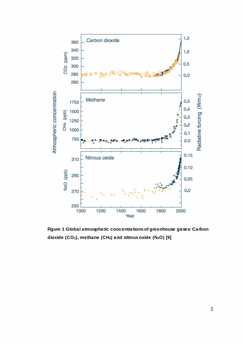
Figure 1 Global atmospheric concentrations of greenhouse gases: Carbon dioxide (CO2), methane (CH4) and nitrous oxide (N2O) [9]................................5
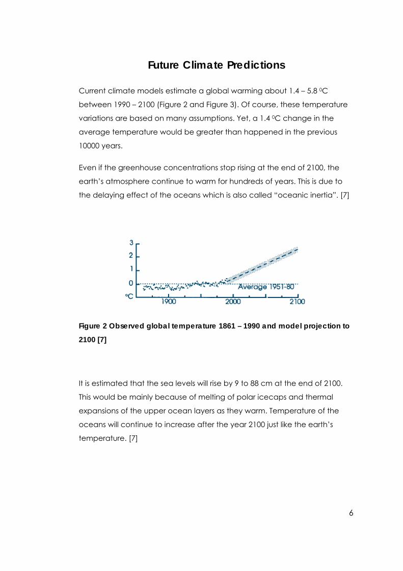
Figure 2 Observed global temperature 1861 – 1990 and model projection to 2100 [7] .........................................................................................................................6
Figure 3 Schematic global temperature from 8000 BC and model projection to 2100 [7] ....................................................................................................................7
Figure 4 Schematic global temperature from 100 million years ago and model projection to 2100 [7] ....................................................................................8
Figure 5 Variation of the earth’s surface temperature for the past 140 years [9] ..................................................................................................................................9
Figure 6 Energy related CO2 emissions by region [10] .......................................10
Figure 7 CO2 Emissions of Turkey in 1980 – 2002 (million tones of CO2) [27] ...11
Figure 8 Increase in CO2 emissions by sector in 2000 – 2030 [10].....................13
Figure 9 Power plant efficiencies after/before removal of CO2. [12] .............18
Figure 10 Power plant emission rates with/without CO2 separation. [12].......18
Figure 11 Global CO2 storage capacities of geological media [10]..............20
Figure 12 Location map of Kuzey Marmara [2] ..................................................26
Figure 13 Structure map of Kuzey Marmara reservoir [2] ..................................27
Figure 14 Initial 3D structure map of Kuzey Marmara field................................36
Figure 15 Final 3D structure map of Kuzey Marmara field.................................37
Figure 16 Dimensions of a single reservoir grid block .........................................38
Figure 17 2D porosity map of Kuzey Marmara reservoir ....................................39
Figure 18 2D permeability map of Kuzey Marmara reservoir ...........................40
Figure 19 Relative permeability chart (krw vs. Sw) ................................................41
Figure 20 Cumulative gas production comparison between field data and simulator results .........................................................................................................54
xvi
Figure 21 Wellhead pressure comparison of KM1 between field data and simulator results .........................................................................................................55
Figure 22 Cumulative gas production comparison of KM1 between field data and simulator results.......................................................................................55
Figure 23 Wellhead pressure comparison of KM3 between field data and simulator results .........................................................................................................56
Figure 24 Cumulative gas production comparison of KM3 between field data and simulator results.......................................................................................56
Figure 25 Wellhead pressure comparison of KM4 between field data and simulator results .........................................................................................................57
Figure 26 Cumulative gas production comparison of KM4 between field data and simulator results.......................................................................................57
Figure 27 Wellhead pressure comparison of KM5 between field data and simulator results .........................................................................................................58
Figure 28 Cumulative gas production comparison of KM5 between field data and simulator results.......................................................................................58
Figure 29 Wellhead pressure comparison of KM6 between field data and simulator results .........................................................................................................59
Figure 30 Cumulative gas production comparison of KM6 between field data and simulator results.......................................................................................59
Figure 31 Scenario 1, CO2 molar fraction distribution of grid layer 1 in 2018-10-01 ...........................................................................................................................63
Figure 32 Scenario 1, CO2 molar fraction distribution of grid layer 5 in 2018-10-01 ...........................................................................................................................63
Figure 33 Scenario 1, CO2 molar fraction distribution of grid layer 1 in the end.....................................................................................................................................64
Figure 34 Scenario 1, CO2 molar fraction distribution of grid layer 5 in the end.....................................................................................................................................64
Figure 35 Scenario 1, average reservoir pressure ...............................................65
Figure 36 Scenario 1, cumulative CO2 injection .................................................65
Figure 37 Scenario 2, CO2 molar fraction distribution of grid layer 1 at production start date ..............................................................................................68
Figure 38 Scenario 2, CO2 molar fraction distribution of grid layer 5 at production start date ..............................................................................................68
xvii
Figure 39 Scenario 2, CO2 molar fraction distribution of grid layer 1 at KM4 shutin date.................................................................................................................69
Figure 40 Scenario 2, CO2 molar fraction distribution of grid layer 5 at KM4 shutin date.................................................................................................................69
Figure 41 Scenario 2, CO2 molar fraction distribution of grid layer 1 at KM1 shutin date.................................................................................................................70
Figure 42 Scenario 2, CO2 molar fraction distribution of grid layer 5 at KM1 shutin date.................................................................................................................70
Figure 43 Scenario 2, CO2 molar fraction distribution of grid layer 1 in the end.....................................................................................................................................71
Figure 44 Scenario 2, CO2 molar fraction distribution of grid layer 5 in the end.....................................................................................................................................71
Figure 45 Scenario 2, wellhead pressures of producers (KM1 and KM4)........72
Figure 46 Scenario 2, bottomhole pressures of injectors (KM3 and KMNew) 72
Figure 47 Scenario 2, KM1 molar production rates.............................................73
Figure 48 Scenario 2, KM4 molar production rates.............................................73
Figure 49 Scenario 2, average reservoir pressure ...............................................74
Figure 50 Scenario 2, cumulative field injection and production....................74
Figure 51 Scenario 3, CO2 molar fraction distribution of grid layer 1 at production start date ..............................................................................................77
Figure 52 Scenario 3, CO2 molar fraction distribution of grid layer 5 at production start date ..............................................................................................77
Figure 53 Scenario 3, CO2 molar fraction distribution of grid layer 1 at KMNew shutin date..................................................................................................78
Figure 54 Scenario 3, CO2 molar fraction distribution of grid layer 5 at KMNew shutin date..................................................................................................78
Figure 55 Scenario 3, CO2 molar fraction distribution of grid layer 1 at KM3 shutin date.................................................................................................................79
Figure 56 Scenario 3, CO2 molar fraction distribution of grid layer 5 at KM3 shutin date.................................................................................................................79
Figure 57 Scenario 3, CO2 molar fraction distribution of grid layer 1 in the end.....................................................................................................................................80
xviii
Figure 58 Scenario 3, CO2 molar fraction distribution of grid layer 5 in the end.....................................................................................................................................80
Figure 59 Scenario 3, wellhead pressures of producers (KM3 and KMNew)..81
Figure 60 Scenario 3, bottomhole pressure of injectors (KM1 and KM4) ........81
Figure 61 Scenario 3, KM3 molar production rates.............................................82
Figure 62 Scenario 3, KMNew molar production rates ......................................82
Figure 63 Scenario 3, average reservoir pressure ...............................................83
Figure 64 Scenario 3, cumulative field injection and production....................83
Figure 65 Scenario 4, CO2 molar fraction distribution of grid layer 1 before production start ........................................................................................................86
Figure 66 Scenario 4, CO2 molar fraction distribution of grid layer 5 before production start ........................................................................................................86
Figure 67 Scenario 4, CO2 molar fraction distribution of grid layer 1 at KM3 shutin date.................................................................................................................87
Figure 68 Scenario 4, CO2 molar fraction distribution of grid layer 5 at KM3 shutin date.................................................................................................................87
Figure 69 Scenario 4, CO2 molar fraction distribution of grid layer 1 in the end.....................................................................................................................................88
Figure 70 Scenario 4, CO2 molar fraction distribution of grid layer 5 in the end.....................................................................................................................................88
Figure 71 Scenario 4, wellhead pressure of KM3.................................................89
Figure 72 Scenario 4, bottomhole pressure of KMNew......................................89
Figure 73 Scenario 4, KM3 molar production rates.............................................90
Figure 74 Scenario 4, average reservoir pressure ...............................................90
Figure 75 Scenario 4, cumulative field injection and production....................91
Figure 76 Cumulative injections of scenarios ......................................................92
Figure 77 Cumulative productions of scenarios..................................................92
Figure 78 Scenario 2, molar production rates of CO2 and CH4 in KM1........113
Figure 79 Scenario 2, molar production rates of minor gases in KM1 ..........113
Figure 80 Scenario 2, molar production rates of CO2 and CH4 in KM4........114

xix
Figure 81 Scenario 2, molar production rates of minor gases in KM4 ..........114
Figure 82 Scenario 3, molar production rates of CO2 and CH4 in KM3........115
Figure 83 Scenario 3, molar production rates of minor gases in KM3 ..........115
Figure 84 Scenario 3, molar production rates of CO2 and CH4 in KMNew..116
Figure 85 Scenario 3, molar production rates of minor gases in KMNew....116
Figure 86 Scenario 4, molar production rates of CO2 and CH4 in KM3........117
Figure 87 Scenario 4, molar production rates of minor gases in KM3 ..........117
xx
ABBREVIATIONS AND ACRONYMS
2D Two dimensional
3D Three dimensional
C1 CH4 (Methane)
C2 C2H6 (Ethane)
C3 C3H8 (Propane)
CMG Computer Modeling Group
CO2 Carbon dioxide
CSC Power plant fed by coal
EGR Enhanced gas recovery
EOR Enhanced oil recovery
EOS Equation of state
GEM Generalized equation of state model compositional
reservoir simulator
H2S Hydrogen sulfide
HC Hydrocarbon
i – C4 (CH3)2CH-CH3 (Isobutane)
i – C5 (CH3)2CH-C2H5 (Isopentane)
IGCC Integrated coal gasification combined cycle
Inj Injection
xxi
MMscf 106 standard cubic feet
MMscfd 106 standard cubic feet per day
Mscf 103 standard cubic feet
Mscfd 103 standard cubic feet per day
n - C4 C4H10 (n - Butane)
n – C5 C5H12 (n - Pentane)
N/A Not applicable
N2 Nitrogen
NGCC Natural gas combined cycle
OD Outer diameter
OGIP Original gas in place
OOIP Original oil in place
OSC Power plant fed by oil
OWIP Original water in place
PF Pulverized fuel fired power plants
Prod Production
RMSE Root mean square error
scf Standard cubic feet
Sl Liquid saturation
Sw Water saturation
TPAO Türkiye Petrolleri Anonim Ortaklığı

xxii
TVD True vertical depth
1
CHAPTER 1
INTRODUCTION
Carbon dioxide forms less than one percent of the earth’s atmosphere
together with the rest of the greenhouse gases [17]. Existence of these
gases keeps the earth warm and even little variations in the atmospheric
concentrations triggers a change in climate.
The world’s temperature has increased less than 1 0C since the beginning of
human civilization and global temperatures had risen about 0.6 0C during
the industrial revolution. It is estimated that current rate of greenhouse gas
emissions will lead to a 1.4 0C temperature increase in the following century.
Historical findings indicate mass extinction events every time the earth faces
a temperature change in such a short period of time. [7]
The seriousness of the situation had already called the attention of many
countries. Conferences and protocols about climate change continue to
be held since 1979. Many of the countries have agreed on reducing their
greenhouse gas emissions in the following years but there are still countries
that haven’t completed their industrial revolution and did not take part in
such emission reduction agreements. [7]
The problem arose from the energy requirements for production. Mass
production facilities require less human crew but much more energy to
operate. Energy is supplied from power plants. Since cost per unit of energy
is a great concern for developing countries, they prefer cheap ways of
producing electricity with the cost of damaging environment. Today, about
half of the world’s carbon dioxide emissions result from power plants and
half of the power plant emissions arose from coal fired power plants. [7, 10,
11]

2
Preventing whole world’s carbon dioxide emissions would not be an
ultimate solution even if it was possible and yet, preventing all the
greenhouse gas emissions will not change the world’s climate immediately.
[7]
Sequestering carbon dioxide into underground offers a way of reducing its
atmospheric concentrations. Underground media includes depleted gas
and oil reservoirs, deep saline aquifers and coal beds. Alternatively ocean
floors can store very large quantities of carbon dioxide.
Kuzey Marmara reservoir is a depleted gas reservoir which is also a
candidate for future gas storage projects. The field is located about 2.5km
away from Silivri coast. Availability of data makes this field a good example
for planning and running simulations concerned with carbon dioxide
sequestration. [1]
Kuzey Marmara reservoir will be the center of attention in this study. It will be
modeled in CMG-GEM simulator and scenarios will be prepared to get the
most out of this reservoir. One additional well is going to be drilled in far
region of the field. Four scenarios will be prepared using previous wells
together with the newly drilled well. Scenario alterations will be formed by
creating variations among well types and surface flow rates. Simulation
results will be evaluated according to the amount of sequestrated carbon
dioxide and produced natural gas.
Before proceeding further in this study, it must be kept in mind that
sequestering carbon dioxide into underground media is like sweeping the
dirt of a room under a carpet. It is rather a workaround than a complete
solution. An ultimate solution will be to include the carbon dioxide into one
of the steps of the carbon cycle such as encouraging forestation or
reducing the amount of fossil fuels burned.

3
CHAPTER 2
LITERATURE REVIEW
Greenhouse Effect
The earth’s atmosphere is a mixture of gases which is mainly formed up of
nitrogen and oxygen. Carbon dioxide, methane, water vapor, ozone,
nitrous oxide and industrial gases forms less than one percent of the
atmosphere and even this amount is enough to keep earth’s surface 30 0C
warmer than otherwise be. [7]
Sun keeps supplying energy to earth mainly in the form of visible light. 30% of
this energy is immediately reflected back to space and the remaining 70%
passes through the atmosphere and warms the earth. Unlike the sun, earth
can not emit this energy as visible light. Instead it emits this energy in the
form of infrared or thermal radiation. Greenhouse gases prevent infrared
radiation from escaping directly to the space. Most of this energy is carried
by air currents to higher levels of the atmosphere and released to space. [7]
Sun’s energy input is distributed between the space and earth’s climate.
Thicker layers of greenhouse gases result a reduction in energy loss to
space. The energy balance is always kept constant. Energy that remains
trapped due to greenhouse gases is used to warm up the climate. [7]
Greenhouse Gases
Apart from the industrial gases, greenhouse gases have been present in the
atmosphere for millions of years. Humans have affected the balance of
these gases by introducing new sources. This supplementary increase in the
4
sources caused an increase in the greenhouse gas releases which is also
known as the “enhanced greenhouse effect”. [7]
Water vapor is the largest contributor to the greenhouse effect but its
amount in the atmosphere is not directly dependent on human activities.
Rising amount of greenhouse gases trigger an increase in the temperature
of weather and warmer weather can hold greater amounts of water vapor
causing an additional impact to the greenhouse effect. [7]
Carbon dioxide emissions contribute 60% of the enhanced greenhouse
effect. This gas naturally occurs in the atmosphere but human activities such
as burning fossil fuels and deforestation releases the carbon in their
structure, sending them to the atmosphere. [7]
During the 10000 years before the industrial revolution, the carbon dioxide
levels varied about 10% whereas a variation of 30% was observed in 200
years period between 1800 and 2000 (Figure 1). With these high rates of
carbon dioxide releases, it is predicted that the levels will continue to rise
about 10% in every passing 20 years. [7]
Methane emissions are responsible for 20% of the greenhouse effect. Its
amount in the atmosphere has started to increase recently but its increment
rate is quite fast. During the industrial era its level has increased 50% (Figure
1). The atmospheric lifetime of methane is 12 years, making this emission a
little less dangerous when compared to carbon dioxide which has an
atmospheric lifetime between 5 to 200 years. [7, 26]
The remaining 20% enhanced greenhouse gas effect is formed by nitrous
oxide, ozone and a number of industrial gases. Nitrous oxide levels have
risen about 16% in recent years (Figure 1). Although some of the industrial
gas levels such as chlorofluorocarbons have been reduced by taken
precautions, there are still long lived gases that their concentrations are
continuously increasing. On the other hand, ozone concentrations are
increasing in some lower portions of the atmosphere although its
concentration tends to decrease globally. [7]
5
Figure 1 Global atmospheric concentrations of greenhouse gases: Carbon
dioxide (CO2), methane (CH4) and nitrous oxide (N2O) [9]
6
Future Climate Predictions
Current climate models estimate a global warming about 1.4 – 5.8 0C
between 1990 – 2100 (Figure 2 and Figure 3). Of course, these temperature
variations are based on many assumptions. Yet, a 1.4 0C change in the
average temperature would be greater than happened in the previous
10000 years.
Even if the greenhouse concentrations stop rising at the end of 2100, the
earth’s atmosphere continue to warm for hundreds of years. This is due to
the delaying effect of the oceans which is also called “oceanic inertia”. [7]
Figure 2 Observed global temperature 1861 – 1990 and model projection to
2100 [7]
It is estimated that the sea levels will rise by 9 to 88 cm at the end of 2100.
This would be mainly because of melting of polar icecaps and thermal
expansions of the upper ocean layers as they warm. Temperature of the
oceans will continue to increase after the year 2100 just like the earth’s
temperature. [7]
7
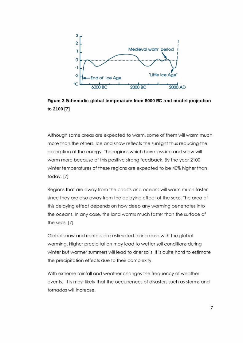
Figure 3 Schematic global temperature from 8000 BC and model projection
to 2100 [7]
Although some areas are expected to warm, some of them will warm much
more than the others. Ice and snow reflects the sunlight thus reducing the
absorption of the energy. The regions which have less ice and snow will
warm more because of this positive strong feedback. By the year 2100
winter temperatures of these regions are expected to be 40% higher than
today. [7]
Regions that are away from the coasts and oceans will warm much faster
since they are also away from the delaying effect of the seas. The area of
this delaying effect depends on how deep any warming penetrates into
the oceans. In any case, the land warms much faster than the surface of
the seas. [7]
Global snow and rainfalls are estimated to increase with the global
warming. Higher precipitation may lead to wetter soil conditions during
winter but warmer summers will lead to drier soils. It is quite hard to estimate
the precipitation effects due to their complexity.
With extreme rainfall and weather changes the frequency of weather
events. It is most likely that the occurrences of disasters such as storms and
tornados will increase.
8
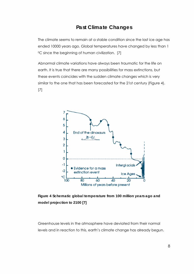
Past Climate Changes
The climate seems to remain at a stable condition since the last ice age has
ended 10000 years ago. Global temperatures have changed by less than 1 0C since the beginning of human civilization. [7]
Abnormal climate variations have always been traumatic for the life on
earth. It is true that there are many possibilities for mass extinctions, but
these events coincides with the sudden climate changes which is very
similar to the one that has been forecasted for the 21st century (Figure 4).
[7]
Figure 4 Schematic global temperature from 100 million years ago and
model projection to 2100 [7]
Greenhouse levels in the atmosphere have deviated from their normal
levels and in reaction to this, earth’s climate change has already begun.
9
This means that the climate change will continue until greenhouse gas
levels keep raising.
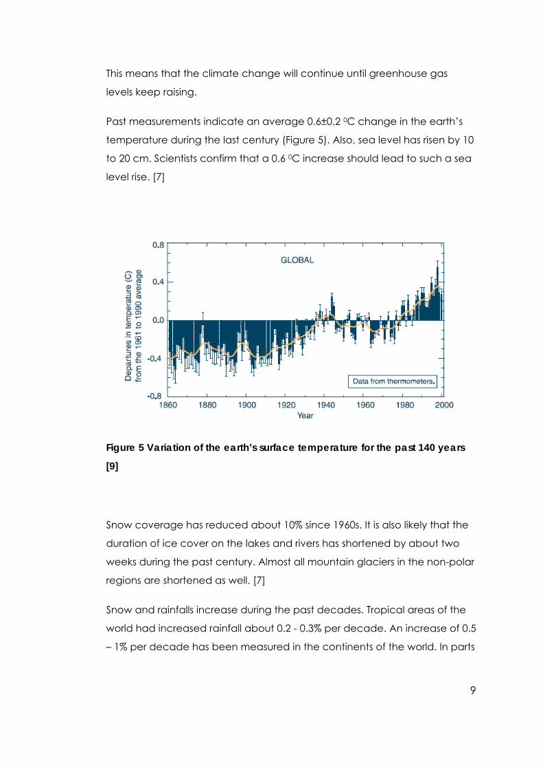
Past measurements indicate an average 0.6±0.2 0C change in the earth’s
temperature during the last century (Figure 5). Also, sea level has risen by 10
to 20 cm. Scientists confirm that a 0.6 0C increase should lead to such a sea
level rise. [7]
Figure 5 Variation of the earth’s surface temperature for the past 140 years
[9]
Snow coverage has reduced about 10% since 1960s. It is also likely that the
duration of ice cover on the lakes and rivers has shortened by about two
weeks during the past century. Almost all mountain glaciers in the non-polar
regions are shortened as well. [7]
Snow and rainfalls increase during the past decades. Tropical areas of the
world had increased rainfall about 0.2 - 0.3% per decade. An increase of 0.5
– 1% per decade has been measured in the continents of the world. In parts
10
of Africa and Asia the frequency and intensity of the droughts seem to have
worsened. [7]
Energy Concern
Energy Related CO2 Emissions
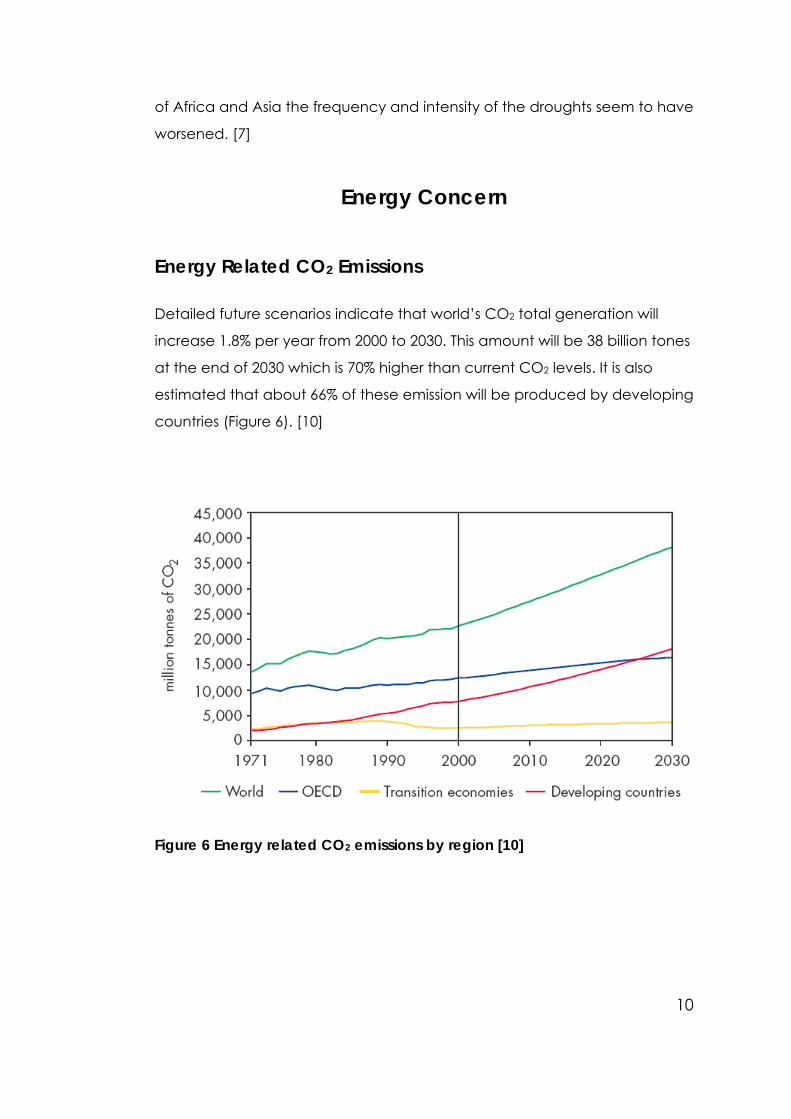
Detailed future scenarios indicate that world’s CO2 total generation will
increase 1.8% per year from 2000 to 2030. This amount will be 38 billion tones
at the end of 2030 which is 70% higher than current CO2 levels. It is also
estimated that about 66% of these emission will be produced by developing
countries (Figure 6). [10]
Figure 6 Energy related CO2 emissions by region [10]
11
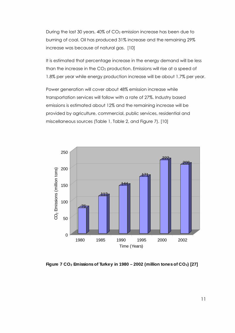
During the last 30 years, 40% of CO2 emission increase has been due to
burning of coal. Oil has produced 31% increase and the remaining 29%
increase was because of natural gas. [10]
It is estimated that percentage increase in the energy demand will be less
than the increase in the CO2 production. Emissions will rise at a speed of
1.8% per year while energy production increase will be about 1.7% per year.
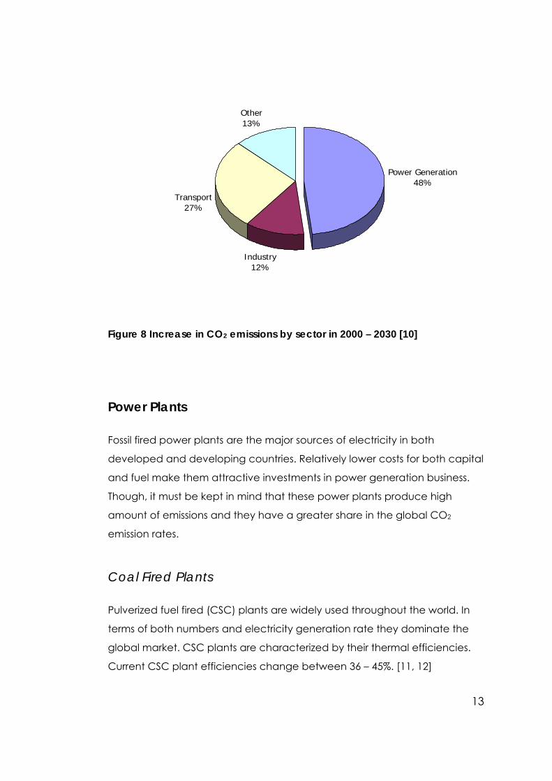
Power generation will cover about 48% emission increase while
transportation services will follow with a rate of 27%. Industry based
emissions is estimated about 12% and the remaining increase will be
provided by agriculture, commercial, public services, residential and
miscellaneous sources (Table 1, Table 2, and Figure 7). [10]
76
113
144
171
222208
0
50
100
150
200
250
CO2
Emis
sion
s (m
illio
n to
ns)
1980 1985 1990 1995 2000 2002Time (Years)
Figure 7 CO2 Emissions of Turkey in 1980 – 2002 (million tones of CO2) [27]
12
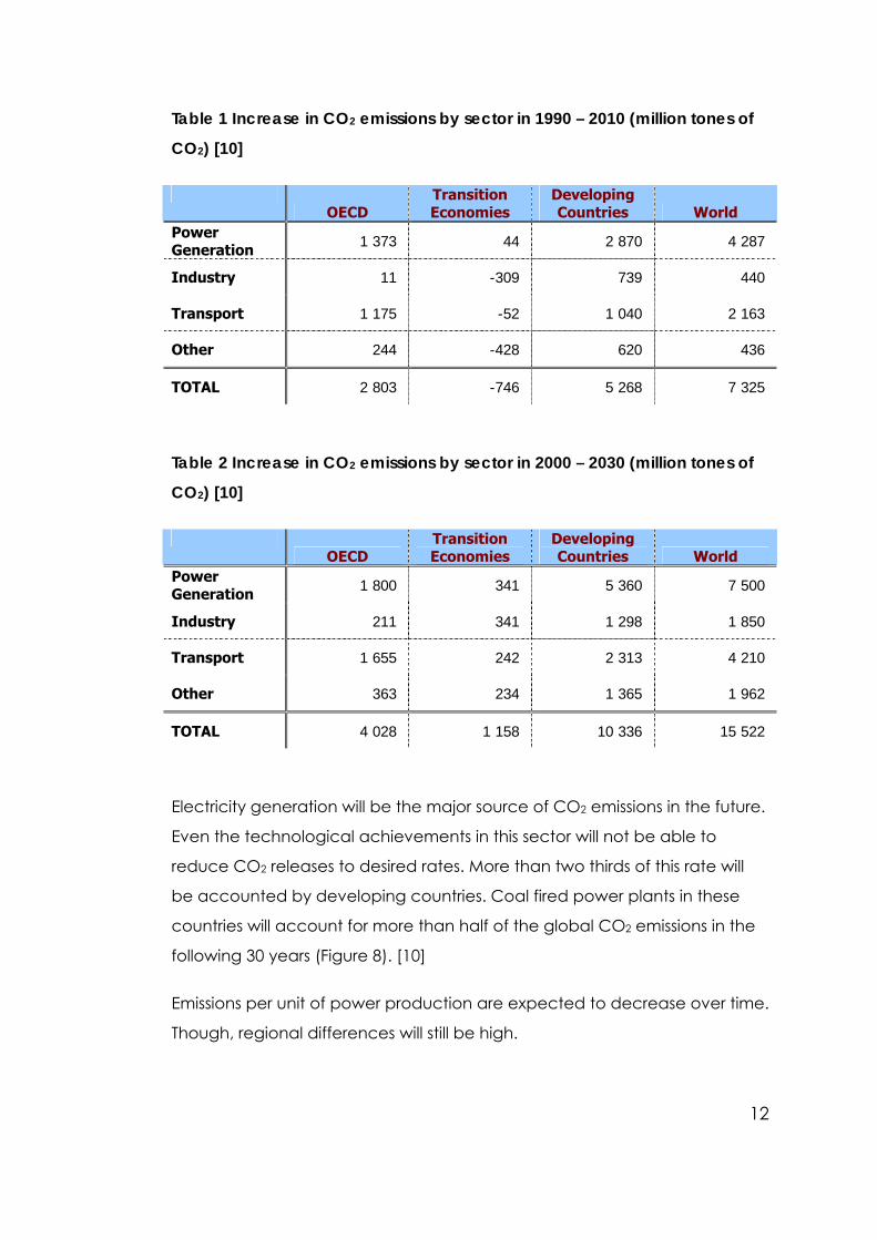
Table 1 Increase in CO2 emissions by sector in 1990 – 2010 (million tones of
CO2) [10]
OECD
Transition Economies
Developing Countries World
Power Generation 1 373 44 2 870 4 287
Industry 11 -309 739 440
Transport 1 175 -52 1 040 2 163
Other 244 -428 620 436
TOTAL 2 803 -746 5 268 7 325
Table 2 Increase in CO2 emissions by sector in 2000 – 2030 (million tones of
CO2) [10]
OECD
Transition Economies
Developing Countries World
Power Generation 1 800 341 5 360 7 500
Industry 211 341 1 298 1 850
Transport 1 655 242 2 313 4 210
Other 363 234 1 365 1 962
TOTAL 4 028 1 158 10 336 15 522
Electricity generation will be the major source of CO2 emissions in the future.
Even the technological achievements in this sector will not be able to
reduce CO2 releases to desired rates. More than two thirds of this rate will
be accounted by developing countries. Coal fired power plants in these
countries will account for more than half of the global CO2 emissions in the
following 30 years (Figure 8). [10]
Emissions per unit of power production are expected to decrease over time.
Though, regional differences will still be high.
13
Power Generation48%
Industry12%
Transport27%
Other13%
Figure 8 Increase in CO2 emissions by sector in 2000 – 2030 [10]
Power Plants
Fossil fired power plants are the major sources of electricity in both
developed and developing countries. Relatively lower costs for both capital
and fuel make them attractive investments in power generation business.
Though, it must be kept in mind that these power plants produce high
amount of emissions and they have a greater share in the global CO2
emission rates.
Coal Fired Plants
Pulverized fuel fired (CSC) plants are widely used throughout the world. In
terms of both numbers and electricity generation rate they dominate the
global market. CSC plants are characterized by their thermal efficiencies.
Current CSC plant efficiencies change between 36 – 45%. [11, 12]
14
In these power plants pulverized coal is burned to obtain a high pressure
steam and the steam is then passed through a steam turbine to produce
electricity. [11]
Another type of coal fired power plant is the integrated gasification
combined cycle (IGCC) plants which have higher efficiency rates even
with low quality coals. Unlike the CSC plants, these plants are not widely in
use. [11, 12]
Coal is mixed with steam and air in a gasifier to produce a fuel gas that
primarily consists of carbon monoxide and hydrogen. The gas is burned in a
gas turbine to produce electricity. High temperature exhaust gas is then
used to operate a separate steam cycle to produce additional electricity.
[11]
Natural Gas Fired Power Plants
Natural gas power plants are suitable for various configurations. Natural gas
combined cycle (NGCC) power plant type is one of the most common
designs that is used to produce electricity. Natural gas is burned in a gas
turbine and the hot exhaust gas is used to drive a steam turbine. These two
combined cycles result an increase in the output efficiency. [11]
Oil Fired Power Plants
Oil and air mixture is sprayed and burned in a furnace to produce heat. The
heat is used to obtain high pressure steam and drive the steam cycle. If
waste heat can be recovered than another steam cycle can be
implemented forming a combined cycle (OSC). Oil plant efficiencies vary
between 23 – 40%. [11, 12]
15
CO2 Capture and Sequestration
CO2 Capture
There are a number of solutions present for capturing CO2 from sources.
Each method provides a different mechanism and cost option for various
cases.
Solvent Scrubbing
This is the most common method used to separate CO2 exhaust gases. It
provides high removal rates with the cost of high energy requirements.
The flue gas is cooled and its impurities are removed. It is then send to an
absorption tower and put in contact with an amine solution. The amine
reacts selectively with CO2 forms a loosely bonded compound with CO2.
This compound is pumped into a stripper tower and CO2 is separated from
the amine. Amine is recovered for further CO2 binding and CO2 is obtained.
This method’s capturing efficiency can be as high as 98% and the purity of
separated CO2 is more than 99%. [11, 12]
Cryogenics
CO2 is captured from the flue gases by means of cooling and
condensation. This method is most useful for gases which require high
amounts of CO2 separation. High energy needs reduces the application of
this method. [11]
Membranes
Membrane technology exploits the physical and chemical differences
between the gases and the membrane itself. The diffusion speed of
16
molecules differs through membrane allowing modest amount of
separation through the process. [11, 13]
Membrane technology allows construction of many different designs. Due
to their variable sized and operating conditions, these membrane systems
are preferred for natural gas producing wells that require CO2 reduction.
[13]
Adsorption
Adsorption ability of certain solids can be used for CO2 separation.
However, selectivity of the solids is very low and the capacity of the system
is below the requirements to adept it to a power plant. [11]
Capture Efficiency
Capturing CO2 from flue gases has a cost. The process requires
considerable amount of energy, especially if the processing amount is high.
This required energy is expressed in terms of cost increase per unit of
electricity generated or efficiency loss. Independent of its representation,
companies do not approach the idea sympathetically unless taxation or a
similar sanction is present.
Following table (Table 3) shows typical power plant emission rates and
efficiencies before any of the capturing methods are applied. Even
preferring NGCC plants instead of coal and oil fired power plants results a
reduction in CO2 emission rates. [12]
17
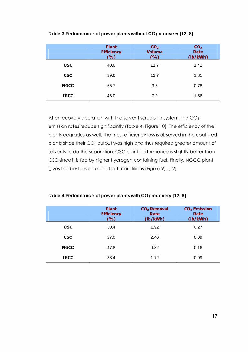
Table 3 Performance of power plants without CO2 recovery [12, 8]
Plant
Efficiency CO2
Volume CO2 Rate
(%) (%) (lb/kWh)
OSC 40.6 11.7 1.42
CSC 39.6 13.7 1.81
NGCC 55.7 3.5 0.78
IGCC 46.0 7.9 1.56
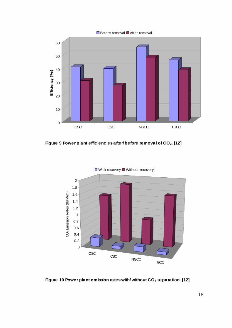
After recovery operation with the solvent scrubbing system, the CO2
emission rates reduce significantly (Table 4, Figure 10). The efficiency of the
plants degrades as well. The most efficiency loss is observed in the coal fired
plants since their CO2 output was high and thus required greater amount of
solvents to do the separation. OSC plant performance is slightly better than
CSC since it is fed by higher hydrogen containing fuel. Finally, NGCC plant
gives the best results under both conditions (Figure 9). [12]
Table 4 Performance of power plants with CO2 recovery [12, 8]
Plant
Efficiency CO2 Removal
Rate CO2 Emission
Rate (%) (lb/kWh) (lb/kWh)
OSC 30.4 1.92 0.27
CSC 27.0 2.40 0.09
NGCC 47.8 0.82 0.16
IGCC 38.4 1.72 0.09
18
0
10
20
30
40
50
60
Effi
cien
cy (
%)
OSC CSC NGCC IGCC
Before removal After removal
Figure 9 Power plant efficiencies after/before removal of CO2. [12]
OSCCSC
NGCCIGCC
0
0.2
0.4
0.6
0.8
1
1.2
1.4
1.6
1.8
2
CO2
Emis
sion
Rat
es (
lb/k
Wh)
With recovery Without recovery
Figure 10 Power plant emission rates with/without CO2 separation. [12]
19
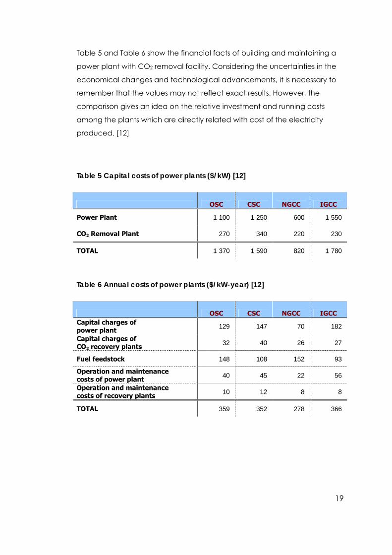
Table 5 and Table 6 show the financial facts of building and maintaining a
power plant with CO2 removal facility. Considering the uncertainties in the
economical changes and technological advancements, it is necessary to
remember that the values may not reflect exact results. However, the
comparison gives an idea on the relative investment and running costs
among the plants which are directly related with cost of the electricity
produced. [12]
Table 5 Capital costs of power plants ($/kW) [12]
OSC CSC NGCC IGCC
Power Plant 1 100 1 250 600 1 550
CO2 Removal Plant 270 340 220 230
TOTAL 1 370 1 590 820 1 780
Table 6 Annual costs of power plants ($/kW-year) [12]
OSC CSC NGCC IGCC Capital charges of power plant 129 147 70 182
Capital charges of CO2 recovery plants 32 40 26 27
Fuel feedstock 148 108 152 93
Operation and maintenance costs of power plant 40 45 22 56
Operation and maintenance costs of recovery plants 10 12 8 8
TOTAL 359 352 278 366
20
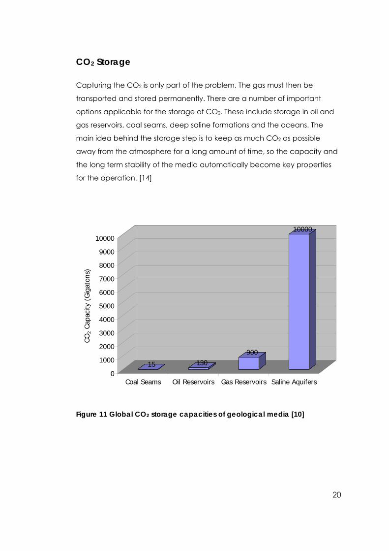
CO2 Storage
Capturing the CO2 is only part of the problem. The gas must then be
transported and stored permanently. There are a number of important
options applicable for the storage of CO2. These include storage in oil and
gas reservoirs, coal seams, deep saline formations and the oceans. The
main idea behind the storage step is to keep as much CO2 as possible
away from the atmosphere for a long amount of time, so the capacity and
the long term stability of the media automatically become key properties
for the operation. [14]
15 130900
10000
0
1000
2000
3000
4000
5000
6000
7000
8000
9000
10000
CO2
Capa
city
(G
igat
ons)
Coal Seams Oil Reservoirs Gas Reservoirs Saline Aquifers
Figure 11 Global CO2 storage capacities of geological media [10]
21
Deep Saline Aquifers
These are underground, water filled layers that are distributed widely below
many major land masses and the oceans. They are generally found in
carbonate or sandstone formations and contain large amounts of saline
water. CO2 can be injected into such reservoirs using techniques similar to
those applied to enhanced oil recovery schemes. Highly saline
underground reservoirs could provide an enormous CO2 storage capacity.
However more experiments in injecting CO2 into aquifers are needed to
gain a better understanding of the process and potential risks. Saline
reservoirs throughout the world might store as much as 10 trillion tones of
CO2, equivalent to more than ten times the total energy related emissions
projected for the next 30 years. [10, 14]
M. Sc. study of Başar Başbuğ demonstrates sequestration of CO2 in a deep
saline aquifer in detail. [31]
Coal Seams
Coal beds represent a large potential geological storage medium for CO2,
with value added benefit. The production of methane, naturally present in
coals, can be enhanced by injecting CO2 into the seam. This displaces the
methane present, which is then drained and used as a valuable fuel source.
Global coal bed storage capacity is estimated at about 15 billion tones.
[14]
Oil and Gas Reservoirs
Reinjecting CO2 into oil fields may lead to enhanced oil recovery, and this
would offset part of the cost of dealing with the gas. Global storage
potential in reservoirs has been estimated at about 1030 billion tones. [10]
22
With EOR, CO2 is injected into operational oil reservoirs in order to increase
the mobility of the oil. As well as boosting or maintaining oil output, much of
the injected CO2 remains trapped in the reservoir. Based on some current
estimates, it is suggested that, globally, 130 billion tons of CO2 could be
stored in this manner. The costs associated with injection of the CO2 can be
compensated from the increased revenue generated from the additional
oil produced. While most of the CO2 currently used for EOR operations is
sourced from naturally occurring CO2 reserves, efforts are continuing to
develop viable, cost effective techniques for utilizing CO2 from sources such
as fossil fuel combustion plants and other major point sources. [14]
It has been suggested that CO2 may have the potential to displace gas
from natural gas fields, maintaining or boosting output. EGR issues are being
investigated as component parts of several major initiatives. These are
looking at development and application of enhanced modeling and
monitoring techniques, reductions in operational costs, site characterization
and mapping, as well as capacity estimation. Another 900 billion tones
could be stored in depleted gas fields. [10, 14]
Oceans
Disposal of CO2 in the ocean might be the solution for regions with no
depleted oil and gas fields or aquifers. The oceans potentially could store all
the carbon in known fossil fuel reserves. Tests are underway on a small scale
to assess the behavior of CO2 dissolved in the ocean and its impact on the
ocean fauna. [10]
It is not yet clear how geological and oceanic systems will react to large-
scale injection of CO2. Key technologies for capture and geological
storage of CO2 have all been tested on an experimental or pilot basis, but
they will be deployed on a commercial scale only if the risks and costs can
be sufficiently reduced and a market value is placed on reducing CO2
emissions. [10]
23
CHAPTER 3
STATEMENT OF THE PROBLEM
Earth’s climate has already begun to change due to the increased amount
of greenhouse gases in the atmosphere. Countries are searching for finding
a way to reduce their emissions. Sequestering carbon dioxide in geological
media provides safe and long term storage conditions.
This study will concentrate on sequestering carbon dioxide into Kuzey
Marmara gas reservoir. Field’s simulation model will be created with CMG
software and reservoir properties will be determined by history matching.
Four different scenarios will be developed in order to find the best
sequestration scheme. Remaining natural gas content of the reservoir will
be produced during the injection of supercritical carbon dioxide.

24
CHAPTER 4
KUZEY MARMARA FIELD
Field History
Kuzey Marmara offshore gas field has been discovered with the drilling of
Kuzey Marmara – 1 well in 1988. This well has been abandoned due to
unsuitable conditions for gas production. Deviated Kuzey Marmara – 2 well
has been drilled from onshore and again abandoned due to very low
permeability and porosity values of the geological structure. [2, 6, 30]
Data from both of the wells have been analyzed and Turkey’s first offshore
field project was initiated. [6]
After careful investigations field’s probable shape has been determined
and the field was planned to be produced with 3 wells at first stage. The
third (Kuzey Marmara – 1/A) well has been drilled 250 ft away from Kuzey
Marmara – 1. Kuzey Marmara – 1/A is located 7 km southwest of Silivri, 2.5
km away from the coast (Figure 11, Figure 12). Kuzey Marmara – 3 and
Kuzey Marmara – 4 were drilled as deviated wells from Kuzey Marmara –
1/A offshore platform. [2, 6, 28, 29, 30]
Taking Kuzey Marmara – 1/A well as origin, Kuzey Marmara – 3 well has
been drilled at location S42.88E 3150 ft and Kuzey Marmara – 4 has been
drilled at the opposite location N33.71W 2550 ft (Figure 13). Drilling of these
wells has been completed at 1995. [1, 6]
During the drilling operations, underground storage options were
considered. Two more wells were drilled to increase the depletion rate in
order to accelerate the utilization of the field for gas storage. These two
25
deviated wells were completed about 1600 ft away from Kuzey Marmara –
1/A platform. The wells were completed in 1996 and the field was put to
commercial production in October 1997. The field was produced with an
unmanned well head platform located at 141 ft water depth. Natural gas
production stopped in 2002 in order to leave the remaining gas as a
cushion for the gas storage. [1, 2, 28, 29]
6 more wells were drilled until 08-05-2003. According to the agreements with
BHI field, Kuzey Marmara – 10 well drilling had started in 05-07-2003 and the
project was completed successfully with the drilling of Kuzey Marmara – 9Z
well in 21-06-2003. [28]
Geology
Kuzey Marmara structure has an elongated shape with major axis striking
from northwest to southeast. It is bounded by two normal faults at east and
west (Figure 13). The reservoir rock is Soğucak formation which consists of
primarily reefal and bioclastic limestone. The top of the reservoir is found at
a depth of 3770 ft. The porosity is about 20% and average water saturation
is about 10%. There is no water gas contact in the reservoir and current
production data do not indicate any aquifer support. Taking the existing
data into account, the reservoir is considered to be volumetric. Average
permeability changes between 20 – 200 md. The thickness of the pay
formation is about 214 ft. At the time of discovery, reservoir pressure was
determined as 2050 psi and average reservoir temperature was 135 0F. [2]
The caprock of the reservoir is Ceylan formation which consists of marl and
tuff with a varying thickness of 30 – 200 ft. [2]
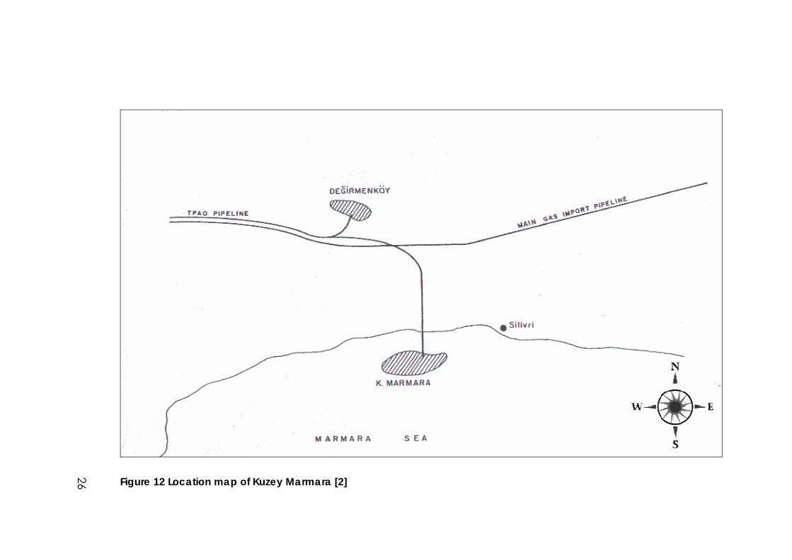
Figure 12 Location map of Kuzey Marmara [2]
26
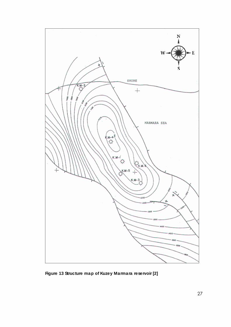
27
Figure 13 Structure map of Kuzey Marmara reservoir [2]
28
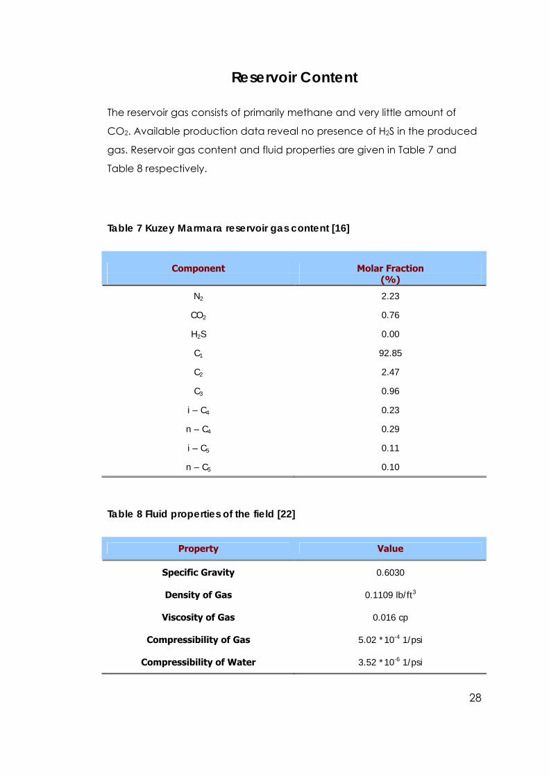
Reservoir Content
The reservoir gas consists of primarily methane and very little amount of
CO2. Available production data reveal no presence of H2S in the produced
gas. Reservoir gas content and fluid properties are given in Table 7 and
Table 8 respectively.
Table 7 Kuzey Marmara reservoir gas content [16]
Component Molar Fraction (%)
N2 2.23
CO2 0.76
H2S 0.00
C1 92.85
C2 2.47
C3 0.96
i – C4 0.23
n – C4 0.29
i – C5 0.11
n – C5 0.10
Table 8 Fluid properties of the field [22]
Property Value
Specific Gravity 0.6030
Density of Gas 0.1109 lb/ft3
Viscosity of Gas 0.016 cp
Compressibility of Gas 5.02 *10-4 1/psi
Compressibility of Water 3.52 *10-6 1/psi
29
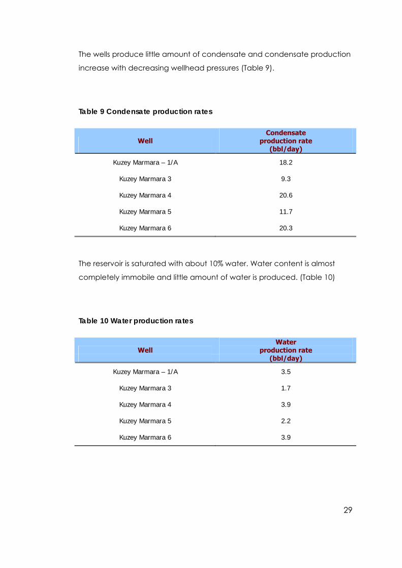
The wells produce little amount of condensate and condensate production
increase with decreasing wellhead pressures (Table 9).
Table 9 Condensate production rates
Well Condensate
production rate (bbl/day)
Kuzey Marmara – 1/A 18.2
Kuzey Marmara 3 9.3
Kuzey Marmara 4 20.6
Kuzey Marmara 5 11.7
Kuzey Marmara 6 20.3
The reservoir is saturated with about 10% water. Water content is almost
completely immobile and little amount of water is produced. (Table 10)
Table 10 Water production rates
Well Water
production rate (bbl/day)
Kuzey Marmara – 1/A 3.5
Kuzey Marmara 3 1.7
Kuzey Marmara 4 3.9
Kuzey Marmara 5 2.2
Kuzey Marmara 6 3.9
30
Gas Storage Project
Kuzey Marmara field’s good characteristic properties make it suitable for
underground gas storage. A feasibility study for converting the field was
performed in 1997. The reservoir and caprock structures were found suitable
for natural gas storage. [2]
In the injection period, natural gas will be withdrawn from the main import
pipeline and measured with the help of a measuring system. With the help
of the compressors the pressure of the gas will be raised according to the
reservoir conditions. The temperature of the compressed gas will be
decreased and the gas will be injected to the reservoir. [2]
In the production interval, gas will be produced and flow to the processing
facilities. Compressors will raise the pressure of the gas to pipeline pressure.
After quality standard measurements, the gas will be transferred to the
pipeline system. [2]

31
CHAPTER 5
METHOD OF SOLUTION
Software
Kuzey Marmara field model was created by using both Computer Modeling
Group’s Generalized Equation of State Model Compositional Reservoir
Simulator and demo version of Golden Software’s Surfer software. Field
equation of state (EOS) model was created using CMG’s WinProp and
integrated into GEM. Properties of CO2 and field gas content were
obtained from WinProp libraries and implemented together with the EOS
data.
Porosity and permeability grids were modeled with the help of Surfer
software and the output data were imported into GEM data file using
Microsoft Excel.
Appendix E contains a valid GEM data file as an example.
Computer Modeling Group (CMG)
CMG is a computer software engineering and consulting firm engaged in
the development, sale and technology transfer of reservoir simulation
software. [19]
CMG began as a company known for its expertise in heavy oil, and
expanded its expertise into all aspects of reservoir flow modeling. Over the
past 20 years, CMG has remained focused on the development and
delivery of reservoir simulation technologies that assist oil and gas
32
companies to determine reservoir capacities and maximize potential
recovery. [19]
Generalized Equation of State Model Compositional
Reservoir Simulator (GEM)
GEM is an efficient, multidimensional, equation of state compositional
simulator which can simulate all the important mechanisms of a miscible
gas injection process, such as vaporization and swelling of oil, condensation
of gas, viscosity and interfacial tension reduction, and the formation of a
miscible solvent bank through multiple contacts. [19, 20]
GEM utilizes either the Peng Robinson or the Soave Redlich Kwong equation
of state to predict the phase equilibrium compositions and densities of the
oil and gas phases, and supports various schemes for computing related
properties such as oil and gas viscosities. [20]
The quasi-Newton successive substitution method is used to solve the
nonlinear equations associated with the flash calculations. A robust stability
test based on a Gibbs energy analysis is used to detect single phase
situations. GEM can align the flash equations with the reservoir flow
equations to obtain an efficient solution of the equations at each time step.
[20]
GEM uses CMG’s grid module for interpreting the reservoir definition
keywords used to describe a complex reservoir. Grids can be of variable
thickness - variable depth type, or be of corner point type, either with or
without user controlled faulting. Other types of grids, such as Cartesian and
cylindrical, are supported as well as locally refined grids of both Cartesian
and hybrid type. [20]
Regional definitions for rock-fluid types, initialization parameters, EOS
parameter types, sector reporting, aquifers are available. Initial reservoir
conditions can be established with given gas-oil and oil-water contact
33
depths. Given proper data fluid composition can be initialized such that it
varies with depth. A linear reservoir temperature gradient may also be
specified.
Aquifers are modeled by either adding boundary cells which contain only
water or by the use of the analytical aquifer model proposed.
WinProp
WinProp is CMG’s equation of state multiphase equilibrium property
package featuring fluid characterization, lumping of components,
matching of laboratory data through regression, simulation of multiple
contact processes, phase diagram construction and solids precipitation.
[19, 21]
WinProp analyzes the phase behavior of reservoir gas and oil systems, and
generate component properties for CMG’s compositional simulator GEM.
[21]
WinProp creates keyword data files to drive the phase behavior calculation
engine. These files contain regular keywords that were required by the
simulator. [21]
Golden Software
Golden Software is one of the leading providers of scientific graphics
software in the world. They develop software for researchers in mining,
engineering, and medicine, as well as thousands of applied scientists and
engineers. [18]
Surfer
Surfer is a contouring and 3D surface mapping program. It converts data
points into contour, surface, wireframe, vector, image, shaded relief, and
34
post maps. Virtually all aspects of maps can be customized to produce the
presentation wanted. [18]
Demo version of Surfer software is fully featured except print, save, copy,
cut, and export functionalities. [18]
Reservoir Model Construction
Production Data
Scaled contour maps and average values of field properties at drilled well
locations were not enough for creating a realistic model of a reservoir. For
this purpose, Kuzey Marmara production data were obtained from
reference “Simulation of Depleted Gas Reservoir for Underground Gas
Storage” [22]. These data were used for generating porosity and
permeability grids and checking the validity of these properties afterwards.
Production information of Kuzey Marmara field between years 1998 – 2002
can be seen in Appendix D. Production tables contain wellhead pressures,
production rate, gas production, condensate production and water
production for each well.
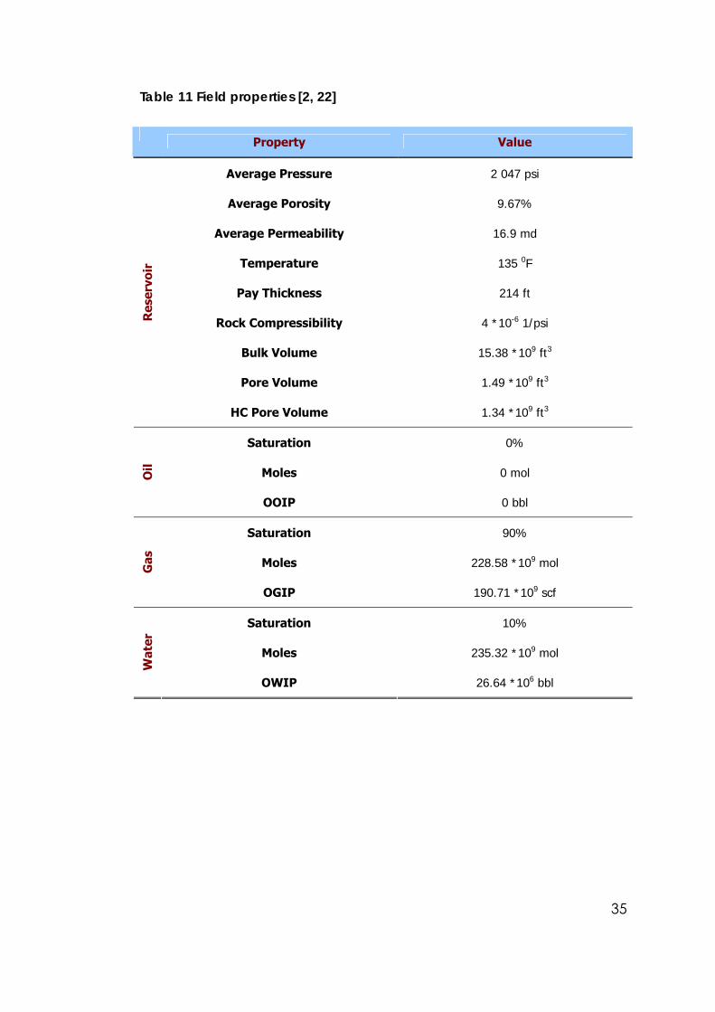
Field
Field property values vary slightly in the publications. The properties
considered in this study are shown in Table 11.
Reservoir properties are the values that obtained at the end of the history
matching simulations. Average reservoir pressure has been changed from
2050 psi to 1050 psi to represent the initial conditions at the beginning of
scenarios.
35
Table 11 Field properties [2, 22]
Property Value
Average Pressure 2 047 psi
Average Porosity 9.67%
Average Permeability 16.9 md
Temperature 135 0F
Pay Thickness 214 ft
Rock Compressibility 4 *10-6 1/psi
Bulk Volume 15.38 *109 ft3
Pore Volume 1.49 *109 ft3
Res
ervo
ir
HC Pore Volume 1.34 *109 ft3
Saturation 0%
Moles 0 mol Oil
OOIP 0 bbl
Saturation 90%
Moles 228.58 *109 mol Gas
OGIP 190.71 *109 scf
Saturation 10%
Moles 235.32 *109 mol
Wat
er
OWIP 26.64 *106 bbl
36
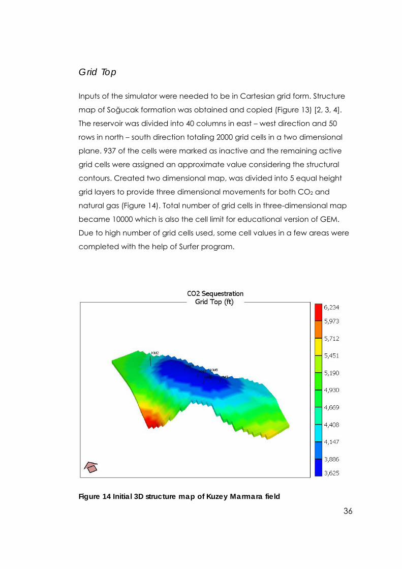
Grid Top
Inputs of the simulator were needed to be in Cartesian grid form. Structure
map of Soğucak formation was obtained and copied (Figure 13) [2, 3, 4].
The reservoir was divided into 40 columns in east – west direction and 50
rows in north – south direction totaling 2000 grid cells in a two dimensional
plane. 937 of the cells were marked as inactive and the remaining active
grid cells were assigned an approximate value considering the structural
contours. Created two dimensional map, was divided into 5 equal height
grid layers to provide three dimensional movements for both CO2 and
natural gas (Figure 14). Total number of grid cells in three-dimensional map
became 10000 which is also the cell limit for educational version of GEM.
Due to high number of grid cells used, some cell values in a few areas were
completed with the help of Surfer program.
Figure 14 Initial 3D structure map of Kuzey Marmara field
37
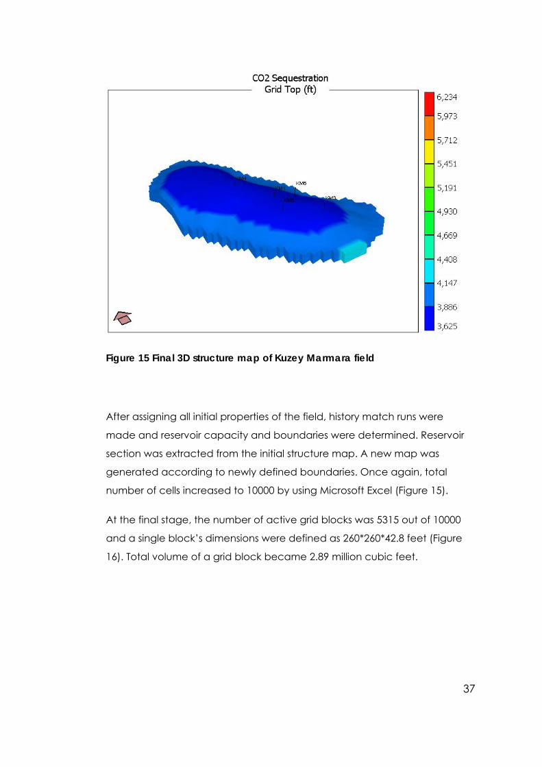
Figure 15 Final 3D structure map of Kuzey Marmara field
After assigning all initial properties of the field, history match runs were
made and reservoir capacity and boundaries were determined. Reservoir
section was extracted from the initial structure map. A new map was
generated according to newly defined boundaries. Once again, total
number of cells increased to 10000 by using Microsoft Excel (Figure 15).
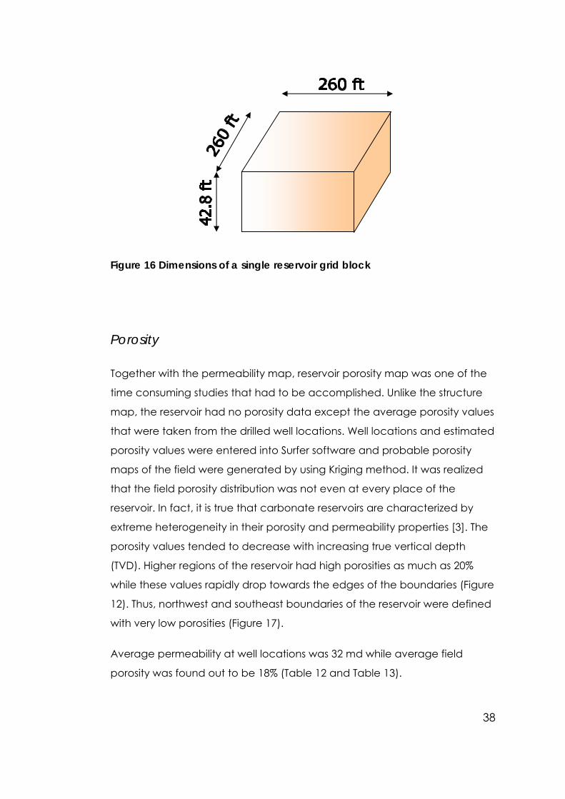
At the final stage, the number of active grid blocks was 5315 out of 10000
and a single block’s dimensions were defined as 260*260*42.8 feet (Figure
16). Total volume of a grid block became 2.89 million cubic feet.
38
Figure 16 Dimensions of a single reservoir grid block
Porosity
Together with the permeability map, reservoir porosity map was one of the
time consuming studies that had to be accomplished. Unlike the structure
map, the reservoir had no porosity data except the average porosity values
that were taken from the drilled well locations. Well locations and estimated
porosity values were entered into Surfer software and probable porosity
maps of the field were generated by using Kriging method. It was realized
that the field porosity distribution was not even at every place of the
reservoir. In fact, it is true that carbonate reservoirs are characterized by
extreme heterogeneity in their porosity and permeability properties [3]. The
porosity values tended to decrease with increasing true vertical depth
(TVD). Higher regions of the reservoir had high porosities as much as 20%
while these values rapidly drop towards the edges of the boundaries (Figure
12). Thus, northwest and southeast boundaries of the reservoir were defined
with very low porosities (Figure 17).
Average permeability at well locations was 32 md while average field
porosity was found out to be 18% (Table 12 and Table 13).
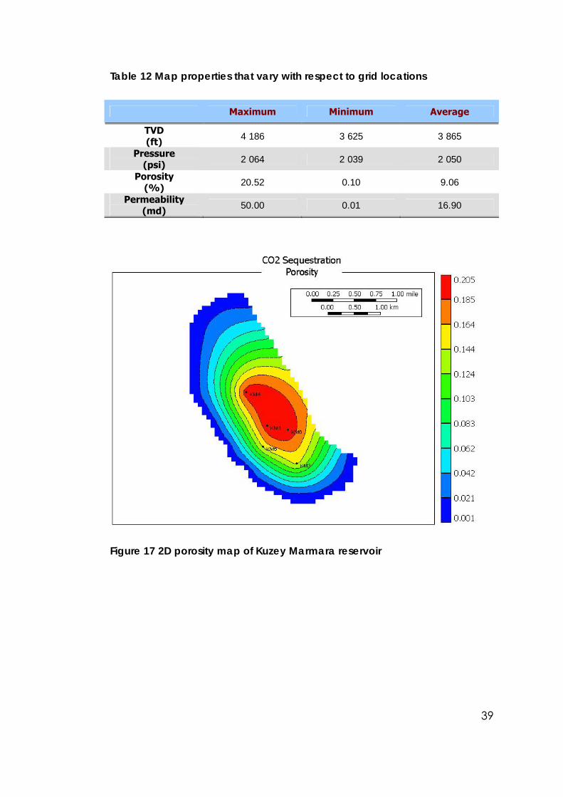
39
Table 12 Map properties that vary with respect to grid locations
Maximum Minimum Average
TVD (ft) 4 186 3 625 3 865
Pressure (psi) 2 064 2 039 2 050
Porosity (%) 20.52 0.10 9.06
Permeability (md) 50.00 0.01 16.90
Figure 17 2D porosity map of Kuzey Marmara reservoir
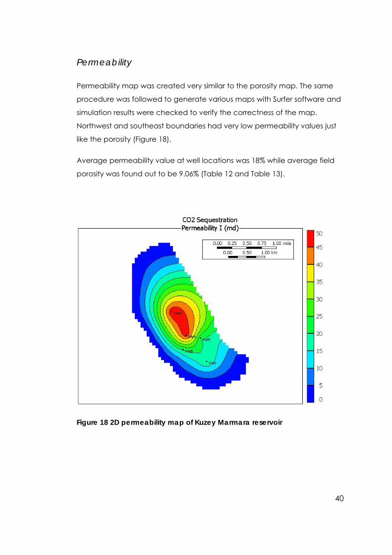
40
Permeability
Permeability map was created very similar to the porosity map. The same
procedure was followed to generate various maps with Surfer software and
simulation results were checked to verify the correctness of the map.
Northwest and southeast boundaries had very low permeability values just
like the porosity (Figure 18).
Average permeability value at well locations was 18% while average field
porosity was found out to be 9.06% (Table 12 and Table 13).
Figure 18 2D permeability map of Kuzey Marmara reservoir
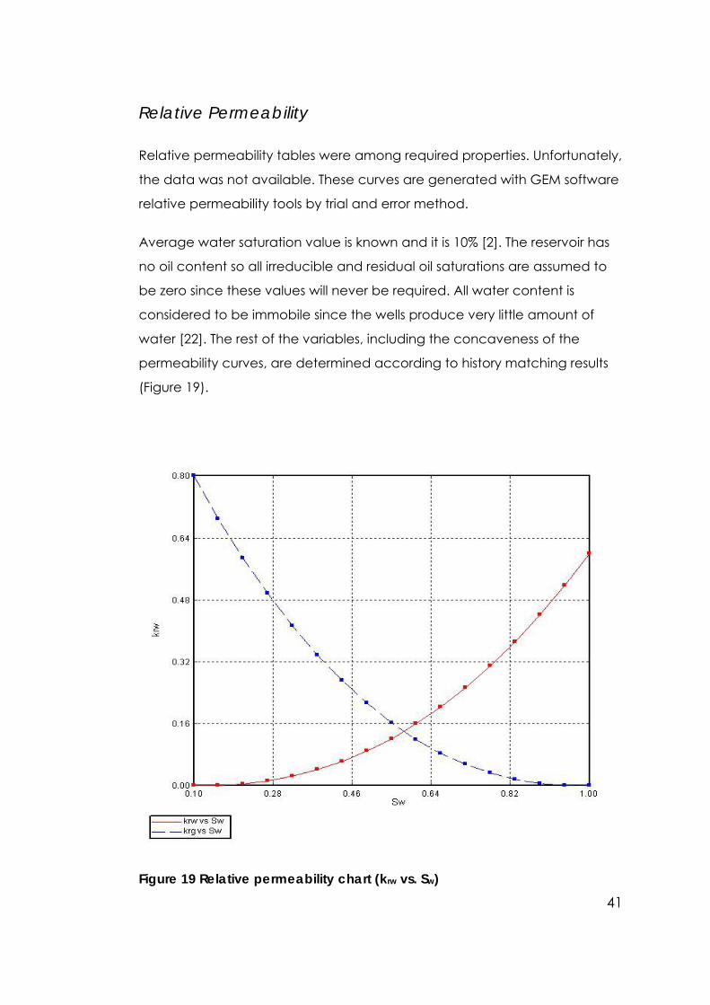
41
Relative Permeability
Relative permeability tables were among required properties. Unfortunately,
the data was not available. These curves are generated with GEM software
relative permeability tools by trial and error method.
Average water saturation value is known and it is 10% [2]. The reservoir has
no oil content so all irreducible and residual oil saturations are assumed to
be zero since these values will never be required. All water content is
considered to be immobile since the wells produce very little amount of
water [22]. The rest of the variables, including the concaveness of the
permeability curves, are determined according to history matching results
(Figure 19).
Figure 19 Relative permeability chart (krw vs. Sw)
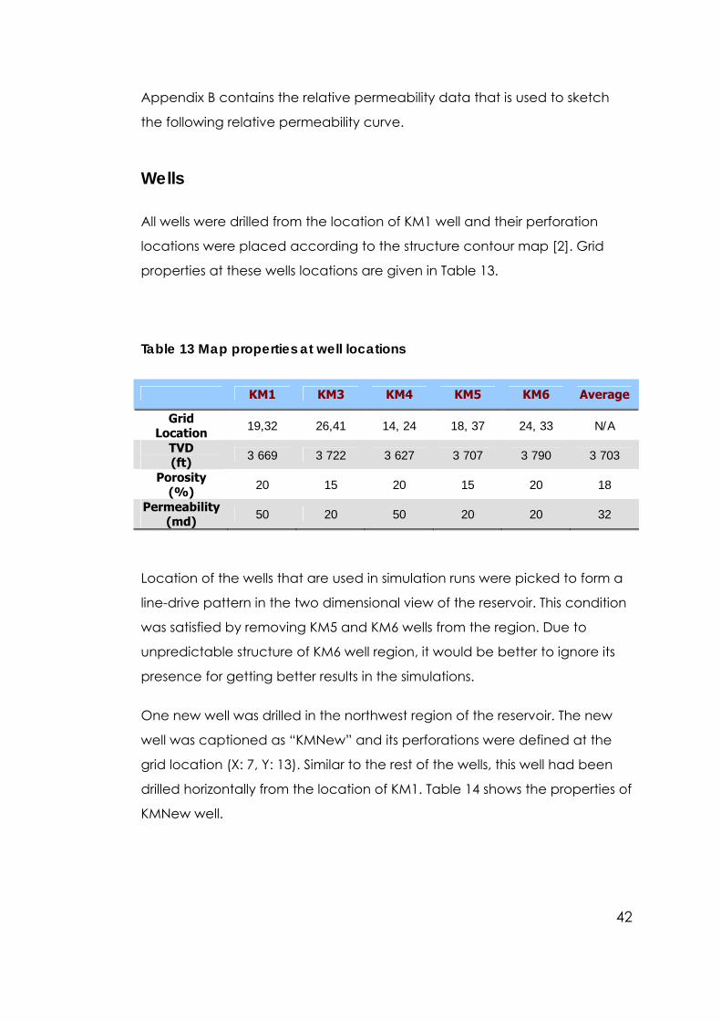
42
Appendix B contains the relative permeability data that is used to sketch
the following relative permeability curve.
Wells
All wells were drilled from the location of KM1 well and their perforation
locations were placed according to the structure contour map [2]. Grid
properties at these wells locations are given in Table 13.
Table 13 Map properties at well locations
KM1 KM3 KM4 KM5 KM6 Average
Grid Location 19,32 26,41 14, 24 18, 37 24, 33 N/A
TVD (ft) 3 669 3 722 3 627 3 707 3 790 3 703
Porosity (%) 20 15 20 15 20 18
Permeability (md) 50 20 50 20 20 32
Location of the wells that are used in simulation runs were picked to form a
line-drive pattern in the two dimensional view of the reservoir. This condition
was satisfied by removing KM5 and KM6 wells from the region. Due to
unpredictable structure of KM6 well region, it would be better to ignore its
presence for getting better results in the simulations.
One new well was drilled in the northwest region of the reservoir. The new
well was captioned as “KMNew” and its perforations were defined at the
grid location (X: 7, Y: 13). Similar to the rest of the wells, this well had been
drilled horizontally from the location of KM1. Table 14 shows the properties of
KMNew well.
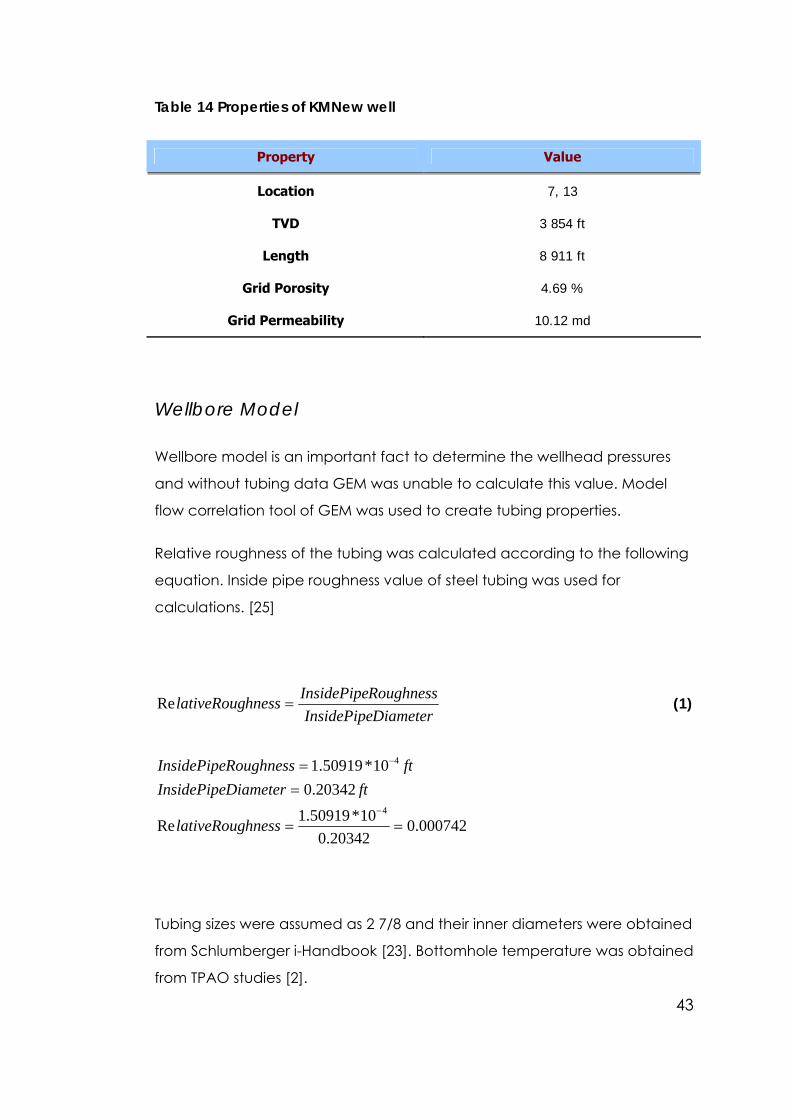
43
Table 14 Properties of KMNew well
Property Value
Location 7, 13
TVD 3 854 ft
Length 8 911 ft
Grid Porosity 4.69 %
Grid Permeability 10.12 md
Wellbore Model
Wellbore model is an important fact to determine the wellhead pressures
and without tubing data GEM was unable to calculate this value. Model
flow correlation tool of GEM was used to create tubing properties.
Relative roughness of the tubing was calculated according to the following
equation. Inside pipe roughness value of steel tubing was used for
calculations. [25]
DiameterInsidePipeRoughnessInsidePipehnesslativeRoug =Re (1)
000742.020342.0
10*50919.1Re
20342.010*50919.1
4
4
==
==
−
−
hnesslativeRoug
ftDiameterInsidePipeftRoughnessInsidePipe
Tubing sizes were assumed as 2 7/8 and their inner diameters were obtained
from Schlumberger i-Handbook [23]. Bottomhole temperature was obtained
from TPAO studies [2].
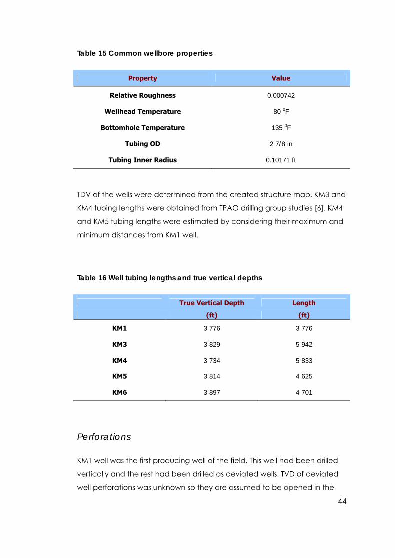
44
Table 15 Common wellbore properties
Property Value
Relative Roughness 0.000742
Wellhead Temperature 80 0F
Bottomhole Temperature 135 0F
Tubing OD 2 7/8 in
Tubing Inner Radius 0.10171 ft
TDV of the wells were determined from the created structure map. KM3 and
KM4 tubing lengths were obtained from TPAO drilling group studies [6]. KM4
and KM5 tubing lengths were estimated by considering their maximum and
minimum distances from KM1 well.
Table 16 Well tubing lengths and true vertical depths
True Vertical Depth Length
(ft) (ft)
KM1 3 776 3 776
KM3 3 829 5 942
KM4 3 734 5 833
KM5 3 814 4 625
KM6 3 897 4 701
Perforations
KM1 well was the first producing well of the field. This well had been drilled
vertically and the rest had been drilled as deviated wells. TVD of deviated
well perforations was unknown so they are assumed to be opened in the
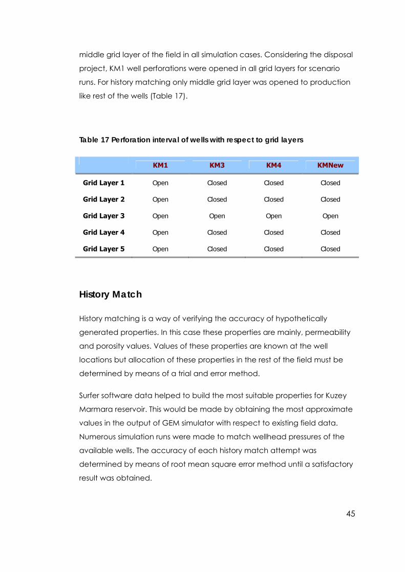
45
middle grid layer of the field in all simulation cases. Considering the disposal
project, KM1 well perforations were opened in all grid layers for scenario
runs. For history matching only middle grid layer was opened to production
like rest of the wells (Table 17).
Table 17 Perforation interval of wells with respect to grid layers
KM1 KM3 KM4 KMNew
Grid Layer 1 Open Closed Closed Closed
Grid Layer 2 Open Closed Closed Closed
Grid Layer 3 Open Open Open Open
Grid Layer 4 Open Closed Closed Closed
Grid Layer 5 Open Closed Closed Closed
History Match
History matching is a way of verifying the accuracy of hypothetically
generated properties. In this case these properties are mainly, permeability
and porosity values. Values of these properties are known at the well
locations but allocation of these properties in the rest of the field must be
determined by means of a trial and error method.
Surfer software data helped to build the most suitable properties for Kuzey
Marmara reservoir. This would be made by obtaining the most approximate
values in the output of GEM simulator with respect to existing field data.
Numerous simulation runs were made to match wellhead pressures of the
available wells. The accuracy of each history match attempt was
determined by means of root mean square error method until a satisfactory
result was obtained.
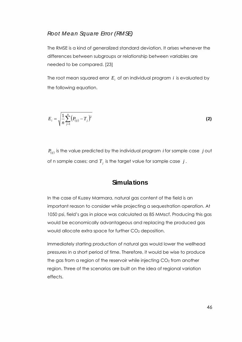
46
Root Mean Square Error (RMSE)
The RMSE is a kind of generalized standard deviation. It arises whenever the
differences between subgroups or relationship between variables are
needed to be compared. [23]
The root mean squared error iE of an individual program i is evaluated by
the following equation.
( )( )∑=
−=n
jjiji TP
nE
1
21 (2)
( )ijP is the value predicted by the individual program i for sample case j out
of n sample cases; and jT is the target value for sample case j .
Simulations
In the case of Kuzey Marmara, natural gas content of the field is an
important reason to consider while projecting a sequestration operation. At
1050 psi, field’s gas in place was calculated as 85 MMscf. Producing this gas
would be economically advantageous and replacing the produced gas
would allocate extra space for further CO2 deposition.
Immediately starting production of natural gas would lower the wellhead
pressures in a short period of time. Therefore, it would be wise to produce
the gas from a region of the reservoir while injecting CO2 from another
region. Three of the scenarios are built on the idea of regional variation
effects.
47
Constraints
Common priority target of these scenarios was to produce the remaining
natural gas in the reservoir as much as possible. Wellhead pressures had to
be kept above 500 psi to make most of the surface equipment work and
the bottomhole pressures had to be above 1070 psi to maintain supercritical
state of CO2.
Kuzey Marmara gas field has been discovered at an average pressure of
about 2050 psi and the maximum average reservoir pressure constraint was
defined as 2300 psi. This was approximately 10% more of the initial reservoir
pressure.
Also, the amount of CO2 percentage in produced gas was an important
constraint. It was aimed that this value must be below 2%. After this value
was reached, a CO2 separator was installed to the system and 2% limitation
was raised to 10% to produce more natural gas from the field.
Assumptions
Practically it is nearly impossible to simulate every detail of a modeled
system due to several reasons. The following characteristics of Kuzey
Marmara reservoir could not be included in the scenarios:
• GEM software had some limitations on the desired runs. Thus, some of the
reservoir parameters could not be included in the simulations. The most
important fact that could not be simulated was the lack of representing
the temperature changes. All scenarios were considered to occur under
isothermal conditions.
• 2004 version of GEM software was not able to handle mineral
interactions within the simulations. CMG company had already declared
implementation of a reaction interface for the upcoming releases.
48
• Provided production data include water and condensate production
rates of the field. GEM software required production ratios with
bottomhole pressures of wells at specific time points to build necessary
tubing tables. Lack of bottomhole pressure information prevented
construction of detailed tubing data. Water and condensate
productions were fairly low so both of them had to be ignored in the
simulations.
• Soğucak limestone is a very variable formation as it is a carbonate type
formation. This kind of formation continuity and thickness patterns are
very complex. This is due to the complexities of processes in the
depositional environment [3]. The properties of the reservoir were
considered to be homogeneous in various situations such as in porosity
and permeability determination.
• Kuzey Marmara reservoir consists of four different layers of formations
which vary in terms of their properties. Absence of well log data
prevented modeling of these formations as separate. All of these layers
were assumed as one single combined layer which shows average
characteristics of actual layers. [1]
• Captured injection fluid was considered to be containing 100% CO2.
Actually, the purity of separated CO2 is about 99%.
• Less than 0.12% of injected CO2 was produced together with the natural
gas after the installation of CO2 separators. Efficiency of the separators
depends on a variety of factors such as temperature, pressure and CO2
percentage of the input gas. Since the separators were assumed virtual
designs, the technical output data was unknown. Cumulative
production results include little amounts of produced but separated CO2
gas.
49
Scenarios
Simulation timelines can be divided into three basic parts.
First one is the “pre injection” period. In this part, assigned injector wells
sequester CO2 while the production wells remains closed. The aim of this
step is to increase the pressure of the reservoir a little so that required
constraints can be satisfied.
Second part is the “natural gas recovery” period. After a suitable reservoir
pressure is reached, production wells are opened and start producing
natural gas while the injector wells continue their CO2 injection. CO2
separators are installed during this period when the CO2 production in the
produced gas exceeds 2%.
Third and final part is the “disposal” period. When the CO2 amount in the
produced gas reaches 10% production wells are shut and converted to
injector wells. Also previous well injection rates are increased.
Table 18 shows information about well injection and production rates for all
scenarios.
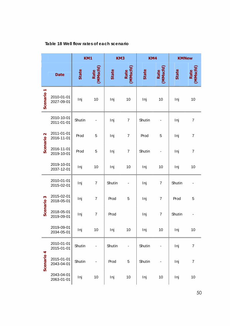
50
Table 18 Well flow rates of each scenario
KM1 KM3 KM4 KMNew
Date St
ate
Rat
e (M
Msc
fd)
Stat
e
Rat
e (M
Msc
fd)
Stat
e
Rat
e (M
Msc
fd)
Stat
e
Rat
e (M
Msc
fd)
Scen
ario
1
2010-01-012027-09-01 Inj 10 Inj 10 Inj 10 Inj 10
2010-10-012011-01-01 Shutin - Inj 7 Shutin - Inj 7
2011-01-012016-11-01 Prod 5 Inj 7 Prod 5 Inj 7
2016-11-012019-10-01 Prod 5 Inj 7 Shutin - Inj 7 Sc
enar
io 2
2019-10-012037-12-01 Inj 10 Inj 10 Inj 10 Inj 10
2010-01-012015-02-01 Inj 7 Shutin - Inj 7 Shutin -
2015-02-012018-05-01 Inj 7 Prod 5 Inj 7 Prod 5
2018-05-012019-09-01 Inj 7 Prod Inj 7 Shutin - Sc
enar
io 3
2019-09-012034-05-01 Inj 10 Inj 10 Inj 10 Inj 10
2010-01-012015-01-01 Shutin - Shutin - Shutin - Inj 7
2015-01-012043-04-01 Shutin - Prod 5 Shutin - Inj 7
Scen
ario
4
2043-04-012063-01-01 Inj 10 Inj 10 Inj 10 Inj 10
51
Scenario 1
This scenario considers immediate injection of CO2 from all of the available
wells. None of the wells produce natural gas and injection rates were
assigned as 10 MM scf/day for each of the wells (Table 18).
This was the simplest CO2 sequestration case that was simulated to
demonstrate the minimum limits of the cumulative injection amount. The
result of Scenario 1 was helpful for making a comparison among the rest of
the simulations.
Scenario 2
In this scenario CO2 deposition was made through both flanks of the
reservoir and the producers were placed in the middle region. Middle
region of the reservoir had higher porosity and permeability values when
compared to the flank regions.
Two of the initial injector rates were assigned as 7 MM scf/day each. One
year after injection has started; two production wells were opened with a
rate of 5 MM scf/day. First CO2 constraint was reached at KM4 well 5 years
and 11 moths after it had started production and the well is shutin. Producer
KM1 reached CO2 constraint after 8 years and 10 months of production
period. Both of the producers were converted to injector wells and all four
well injection rates were assigned as 10 MM scf/day until average reservoir
pressure constraint of 2300 psi was reached (Table 18).
Scenario 3
This scenario is very similar to the Scenario 2 except for the injector and
producer wells types are exchanged. Wells placed in the flanks of the
reservoir were used for production and injector wells were placed in the
middle.
52
Two of the initial injector rates were assigned as 10 MM scf/day. After five
years of injection period, KMNew and KM3 production wells were opened
with production rates of 5 MM scf/day and 4MM scf/day respectively.
KMNew well reached its CO2 constraint after producing for 3 years and 3
months time and was shutin. The other producer, KM3 well, was closed 4
years 7 months after it had started producing. Both of the producers were
converted to injector wells and all their injection rates were assigned as 10
MM scf/day each until average reservoir pressure constraint was reached
(Table 18).
Scenario 4
KMNew well was assigned as injector in the northwest flank of the field. CO2
injection rate was assigned as 7MM scf/day. After 5 years of injection period
KM3 producer was opened in the south eastern flank side and its
production rate was set to 5MM scf/day. Both wells remained open for 28
years and 3 months period. KM4 and KM1 wells were opened as injectors
and the producer KM3 was converted to an injector well. All of the four well
injection rates were set to 10MM scf/day and these wells remained open
until an average reservoir pressure of 2300 psi was reached (Table 18).
Unlike the previous scenarios, the simulation was ended because of
wellhead pressure constraint. CO2 separator was installed when it was
necessary but the produced CO2 amount never reached 10%.
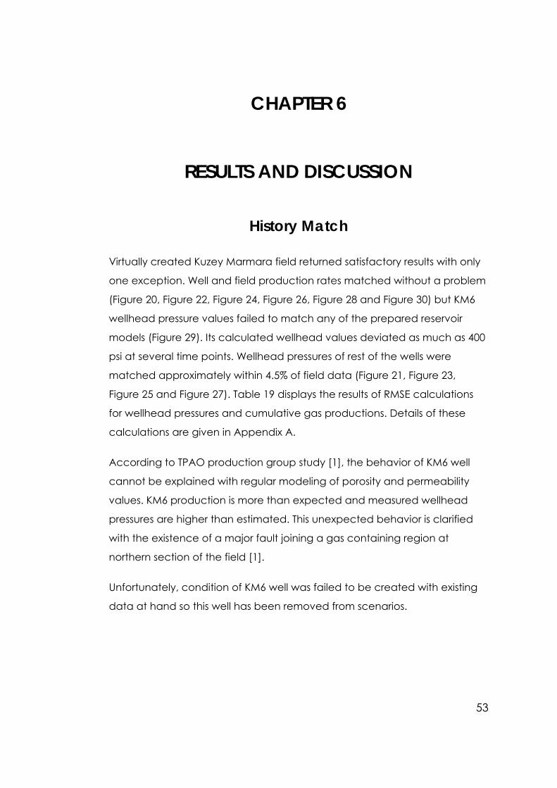
53
CHAPTER 6
RESULTS AND DISCUSSION
History Match
Virtually created Kuzey Marmara field returned satisfactory results with only
one exception. Well and field production rates matched without a problem
(Figure 20, Figure 22, Figure 24, Figure 26, Figure 28 and Figure 30) but KM6
wellhead pressure values failed to match any of the prepared reservoir
models (Figure 29). Its calculated wellhead values deviated as much as 400
psi at several time points. Wellhead pressures of rest of the wells were
matched approximately within 4.5% of field data (Figure 21, Figure 23,
Figure 25 and Figure 27). Table 19 displays the results of RMSE calculations
for wellhead pressures and cumulative gas productions. Details of these
calculations are given in Appendix A.
According to TPAO production group study [1], the behavior of KM6 well
cannot be explained with regular modeling of porosity and permeability
values. KM6 production is more than expected and measured wellhead
pressures are higher than estimated. This unexpected behavior is clarified
with the existence of a major fault joining a gas containing region at
northern section of the field [1].
Unfortunately, condition of KM6 well was failed to be created with existing
data at hand so this well has been removed from scenarios.
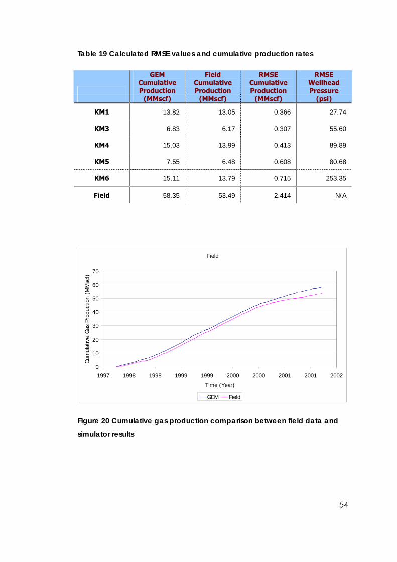
54
Table 19 Calculated RMSE values and cumulative production rates
GEM Cumulative Production
Field Cumulative Production
RMSE Cumulative Production
RMSE Wellhead Pressure
(MMscf) (MMscf) (MMscf) (psi)
KM1 13.82 13.05 0.366 27.74
KM3 6.83 6.17 0.307 55.60
KM4 15.03 13.99 0.413 89.89
KM5 7.55 6.48 0.608 80.68
KM6 15.11 13.79 0.715 253.35
Field 58.35 53.49 2.414 N/A
Field
0
10
20
30
40
50
60
70
1997 1998 1998 1999 1999 2000 2000 2001 2001 2002
Time (Year)
Cum
ulat
ive
Gas
Pro
duct
ion
(MM
scf)
GEM Field
Figure 20 Cumulative gas production comparison between field data and
simulator results
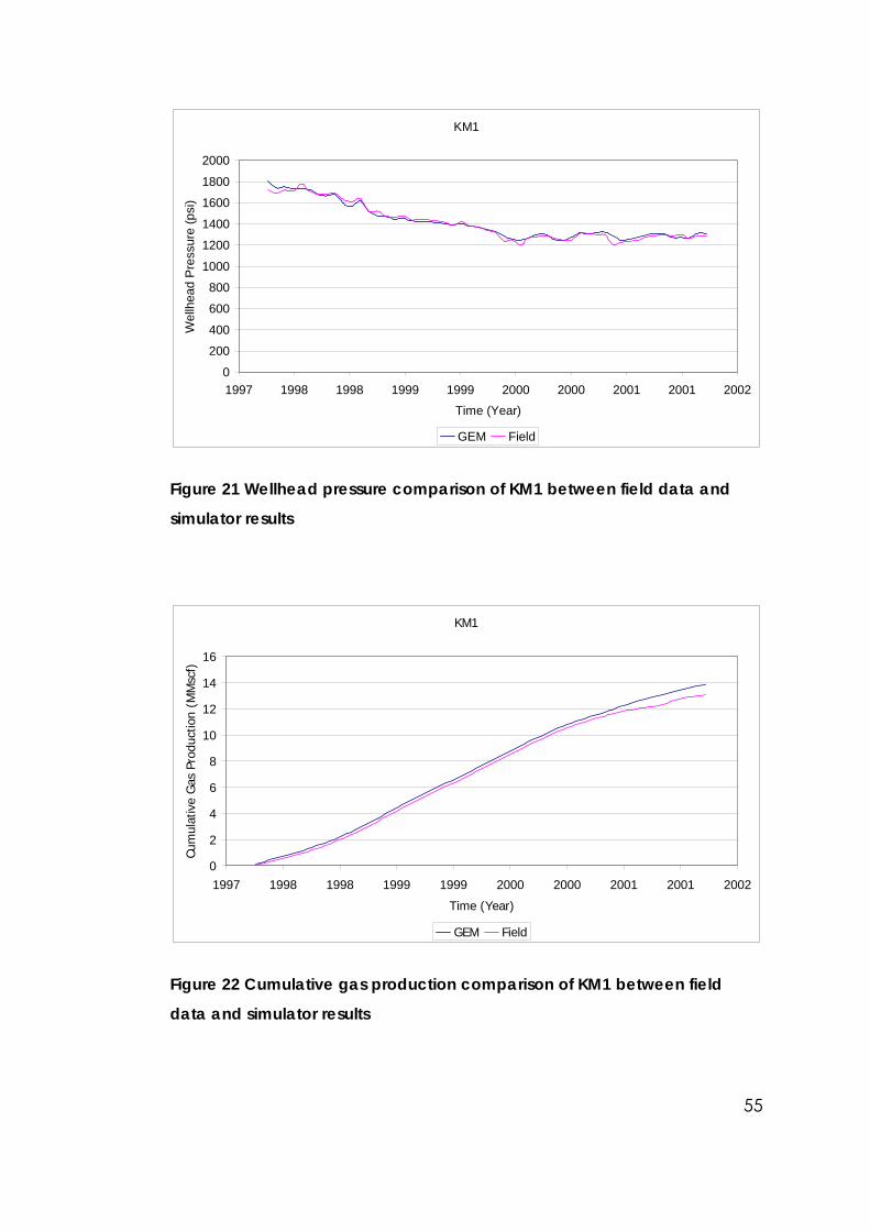
55
KM1
0
200
400
600
800
1000
1200
1400
1600
1800
2000
1997 1998 1998 1999 1999 2000 2000 2001 2001 2002Time (Year)
Wel
lhea
d P
ress
ure
(psi
)
GEM Field
Figure 21 Wellhead pressure comparison of KM1 between field data and
simulator results
KM1
0
2
4
6
8
10
12
14
16
1997 1998 1998 1999 1999 2000 2000 2001 2001 2002
Time (Year)
Cum
ulat
ive
Gas
Pro
duct
ion
(MM
scf)
GEM Field
Figure 22 Cumulative gas production comparison of KM1 between field
data and simulator results
56
KM3
0
200
400
600
800
1000
1200
1400
1600
1800
1997 1998 1998 1999 1999 2000 2000 2001 2001 2002Time (Year)
Wel
lhea
d P
ress
ure
(psi
)
GEM Field
Figure 23 Wellhead pressure comparison of KM3 between field data and
simulator results
KM3
0
1
2
3
4
5
6
7
8
1997 1998 1998 1999 1999 2000 2000 2001 2001 2002
Time (Year)
Cum
ulat
ive
Gas
Pro
duct
ion
(MM
scf)
GEM Field
Figure 24 Cumulative gas production comparison of KM3 between field
data and simulator results
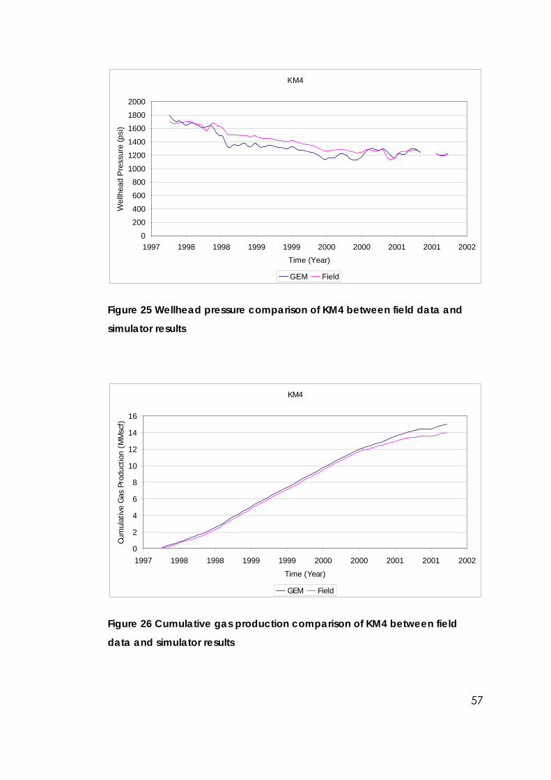
57
KM4
0
200
400
600
800
1000
1200
1400
1600
1800
2000
1997 1998 1998 1999 1999 2000 2000 2001 2001 2002Time (Year)
Wel
lhea
d P
ress
ure
(psi
)
GEM Field
Figure 25 Wellhead pressure comparison of KM4 between field data and
simulator results
KM4
0
2
4
6
8
10
12
14
16
1997 1998 1998 1999 1999 2000 2000 2001 2001 2002
Time (Year)
Cum
ulat
ive
Gas
Pro
duct
ion
(MM
scf)
GEM Field
Figure 26 Cumulative gas production comparison of KM4 between field
data and simulator results
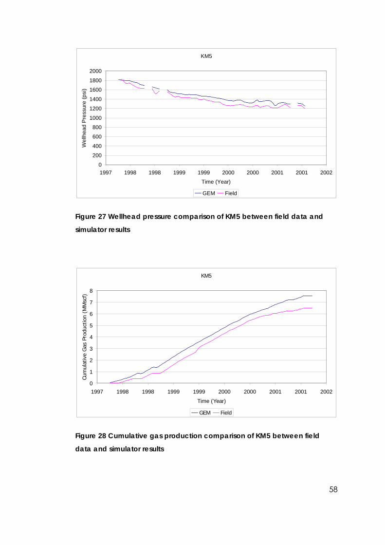
58
KM5
0
200
400
600
800
1000
1200
1400
1600
1800
2000
1997 1998 1998 1999 1999 2000 2000 2001 2001 2002Time (Year)
Wel
lhea
d P
ress
ure
(psi
)
GEM Field
Figure 27 Wellhead pressure comparison of KM5 between field data and
simulator results
KM5
0
1
2
3
4
5
6
7
8
1997 1998 1998 1999 1999 2000 2000 2001 2001 2002
Time (Year)
Cum
ulat
ive
Gas
Pro
duct
ion
(MM
scf)
GEM Field
Figure 28 Cumulative gas production comparison of KM5 between field
data and simulator results
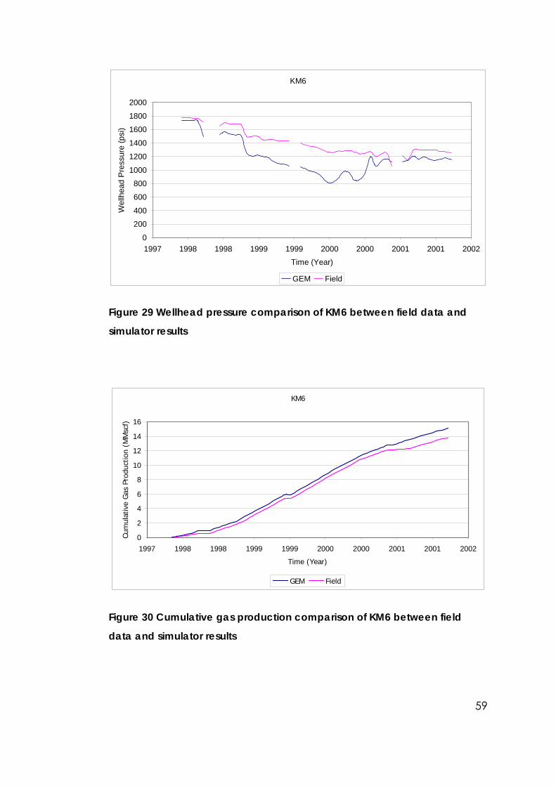
59
KM6
0
200
400
600
800
1000
1200
1400
1600
1800
2000
1997 1998 1998 1999 1999 2000 2000 2001 2001 2002Time (Year)
Wel
lhea
d P
ress
ure
(psi
)
GEM Field
Figure 29 Wellhead pressure comparison of KM6 between field data and
simulator results
KM6
0
2
4
6
8
10
12
14
16
1997 1998 1998 1999 1999 2000 2000 2001 2001 2002
Time (Year)
Cum
ulat
ive
Gas
Pro
duct
ion
(MM
scf)
GEM Field
Figure 30 Cumulative gas production comparison of KM6 between field
data and simulator results
60
Scenarios
Power plants are good sources of CO2 emissions. In fact, daily CO2 gross
emission rate of a 250 MW NGCC power plant is about 40.1 MMscf (4.68
million lb) per day which is barely enough to be sequestered in any of the
scenarios. [12]
Pressure distribution within the reservoir was pretty even. Maximum and
minimum observed pressure differences were about 200 psi at the end of
injection periods.
Scenario 1
This simple injection scenario indicated that in the worst cases Kuzey
Marmara reservoir has the ability to store 258 billion ft3 (30 billion lb) of CO2
at standard conditions (Figure 36).
Table 20 and Table 21 show the numerical results of the scenario. Figure 35
shows average reservoir pressure change during the simulation. CO2
propagation and natural gas movement is displayed through Figure 31 to
Figure 34.
Although the reservoir had no producing wells, injected CO2 was not totally
mixed with natural gas. A mixing zone formed between natural gas and
CO2 and CO2 propagated to the lower levels. Natural gas was withdrawn to
the upper grid layers and compressed due to increasing amount of CO2.
CO2 front velocity was faster in low porosity regions with respect to high
porosity regions. However, CO2 was still prone to moving towards lower grid
layers due to gravitational differences.
KMNew and KM3 wells had the most spread CO2 area throughout the
simulation. This was due to the region of the well which has relatively lower
permeability and porosity values. Lower permeability slowed downward

61
movement and lower porosity increased the front velocity through the grid
layers. Even well regions in the uppermost grid layer had wider area
coverage.
KM1 and KM4 wells were placed in high permeability and high porosity
regions so CO2 propagation was towards the deepest grid layer while the
front velocity was almost none in the uppermost grid layer.
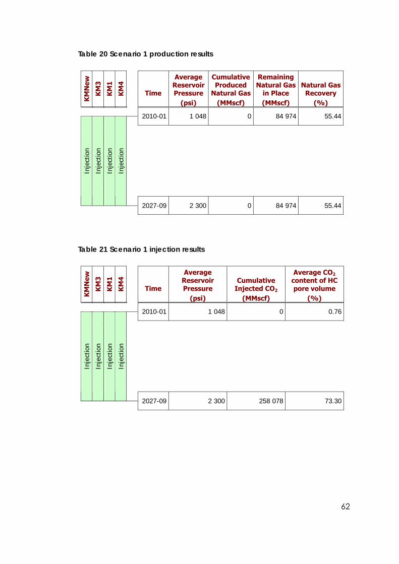
62
Table 20 Scenario 1 production results
Time
Average Reservoir Pressure
Cumulative Produced
Natural Gas
Remaining Natural Gas
in Place Natural Gas
Recovery K
MN
ew
KM
3
KM
1
KM
4
(psi) (MMscf) (MMscf) (%)
2010-01 1 048 0 84 974 55.44
Inje
ctio
n
Inje
ctio
n
Inje
ctio
n
Inje
ctio
n
2027-09 2 300 0 84 974 55.44
Table 21 Scenario 1 injection results
Time
Average Reservoir Pressure
Cumulative Injected CO2
Average CO2 content of HC pore volume
KM
New
KM
3
KM
1
KM
4
(psi) (MMscf) (%)
2010-01 1 048 0 0.76
Inje
ctio
n
Inje
ctio
n
Inje
ctio
n
Inje
ctio
n
2027-09 2 300 258 078 73.30
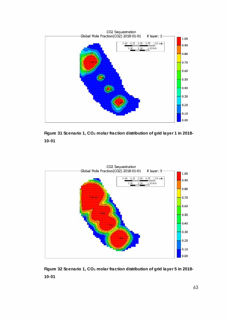
63
Figure 31 Scenario 1, CO2 molar fraction distribution of grid layer 1 in 2018-
10-01
Figure 32 Scenario 1, CO2 molar fraction distribution of grid layer 5 in 2018-
10-01
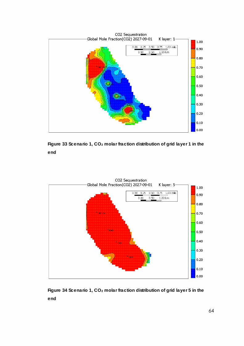
64
Figure 33 Scenario 1, CO2 molar fraction distribution of grid layer 1 in the
end
Figure 34 Scenario 1, CO2 molar fraction distribution of grid layer 5 in the
end
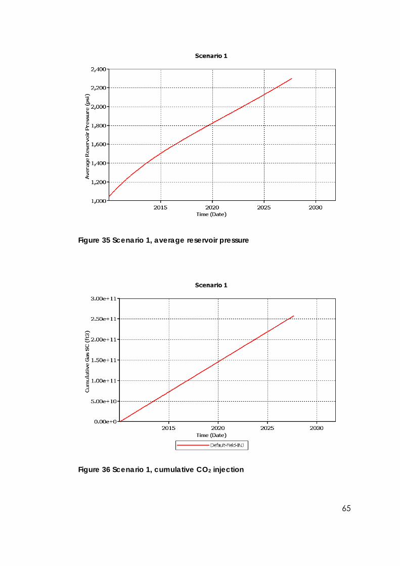
65
Figure 35 Scenario 1, average reservoir pressure
Figure 36 Scenario 1, cumulative CO2 injection
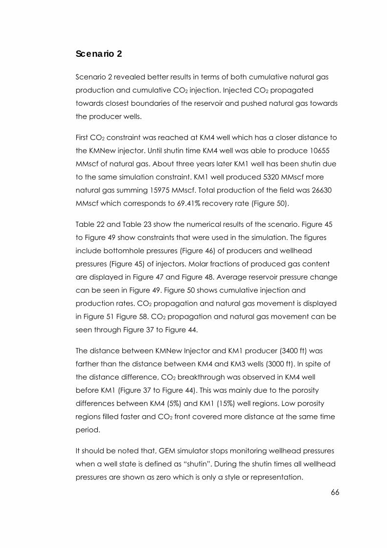
66
Scenario 2
Scenario 2 revealed better results in terms of both cumulative natural gas
production and cumulative CO2 injection. Injected CO2 propagated
towards closest boundaries of the reservoir and pushed natural gas towards
the producer wells.
First CO2 constraint was reached at KM4 well which has a closer distance to
the KMNew injector. Until shutin time KM4 well was able to produce 10655
MMscf of natural gas. About three years later KM1 well has been shutin due
to the same simulation constraint. KM1 well produced 5320 MMscf more
natural gas summing 15975 MMscf. Total production of the field was 26630
MMscf which corresponds to 69.41% recovery rate (Figure 50).
Table 22 and Table 23 show the numerical results of the scenario. Figure 45
to Figure 49 show constraints that were used in the simulation. The figures
include bottomhole pressures (Figure 46) of producers and wellhead
pressures (Figure 45) of injectors. Molar fractions of produced gas content
are displayed in Figure 47 and Figure 48. Average reservoir pressure change
can be seen in Figure 49. Figure 50 shows cumulative injection and
production rates. CO2 propagation and natural gas movement is displayed
in Figure 51 Figure 58. CO2 propagation and natural gas movement can be
seen through Figure 37 to Figure 44.
The distance between KMNew Injector and KM1 producer (3400 ft) was
farther than the distance between KM4 and KM3 wells (3000 ft). In spite of
the distance difference, CO2 breakthrough was observed in KM4 well
before KM1 (Figure 37 to Figure 44). This was mainly due to the porosity
differences between KM4 (5%) and KM1 (15%) well regions. Low porosity
regions filled faster and CO2 front covered more distance at the same time
period.
It should be noted that, GEM simulator stops monitoring wellhead pressures
when a well state is defined as “shutin”. During the shutin times all wellhead
pressures are shown as zero which is only a style or representation.
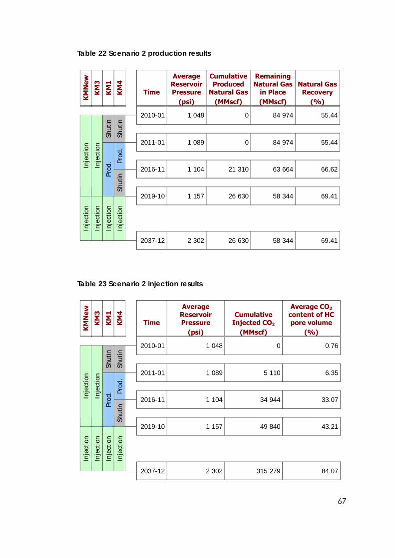
67
Table 22 Scenario 2 production results
Time
Average Reservoir Pressure
Cumulative Produced
Natural Gas
Remaining Natural Gas
in Place Natural Gas
Recovery K
MN
ew
KM
3
KM
1
KM
4
(psi) (MMscf) (MMscf) (%)
2010-01 1 048 0 84 974 55.44
Shut
in
Shut
in
2011-01 1 089 0 84 974 55.44
Prod
.
2016-11 1 104 21 310 63 664 66.62
Inje
ctio
n
Inje
ctio
n
Prod
.
Shut
in
2019-10 1 157 26 630 58 344 69.41
Inje
ctio
n
Inje
ctio
n
Inje
ctio
n
Inje
ctio
n
2037-12 2 302 26 630 58 344 69.41
Table 23 Scenario 2 injection results
Time
Average Reservoir Pressure
Cumulative Injected CO2
Average CO2 content of HC pore volume
KM
New
KM
3
KM
1
KM
4
(psi) (MMscf) (%)
2010-01 1 048 0 0.76
Shut
in
Shut
in
2011-01 1 089 5 110 6.35
Prod
.
2016-11 1 104 34 944 33.07
Inje
ctio
n
Inje
ctio
n
Prod
.
Shut
in
2019-10 1 157 49 840 43.21
Inje
ctio
n
Inje
ctio
n
Inje
ctio
n
Inje
ctio
n
2037-12 2 302 315 279 84.07
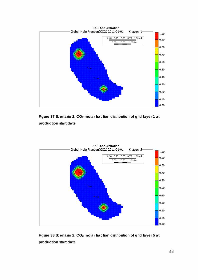
68
Figure 37 Scenario 2, CO2 molar fraction distribution of grid layer 1 at
production start date
Figure 38 Scenario 2, CO2 molar fraction distribution of grid layer 5 at
production start date
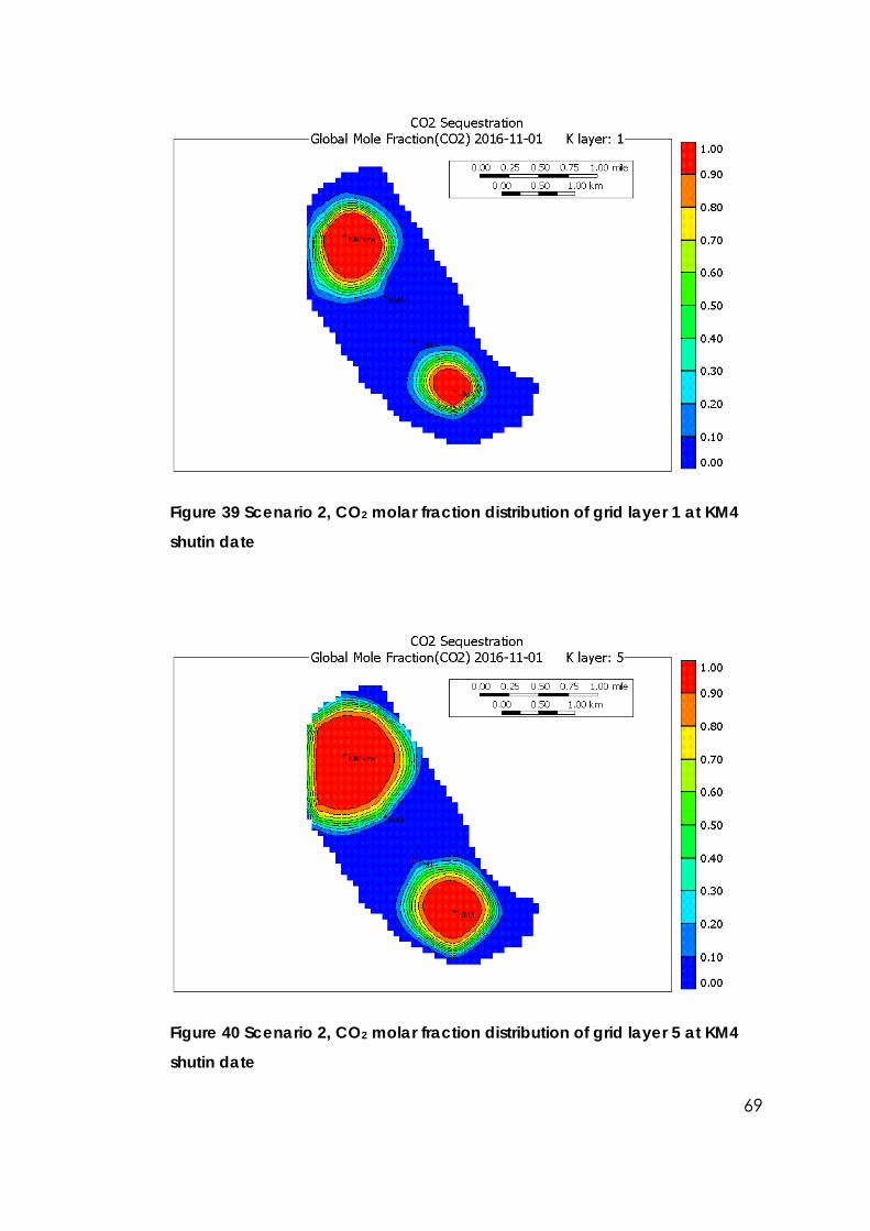
69
Figure 39 Scenario 2, CO2 molar fraction distribution of grid layer 1 at KM4
shutin date
Figure 40 Scenario 2, CO2 molar fraction distribution of grid layer 5 at KM4
shutin date
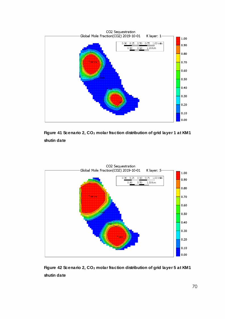
70
Figure 41 Scenario 2, CO2 molar fraction distribution of grid layer 1 at KM1
shutin date
Figure 42 Scenario 2, CO2 molar fraction distribution of grid layer 5 at KM1
shutin date
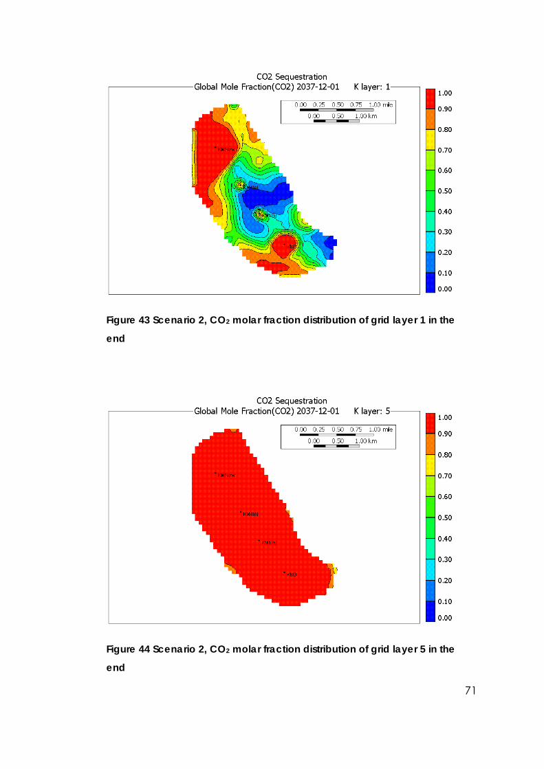
71
Figure 43 Scenario 2, CO2 molar fraction distribution of grid layer 1 in the
end
Figure 44 Scenario 2, CO2 molar fraction distribution of grid layer 5 in the
end
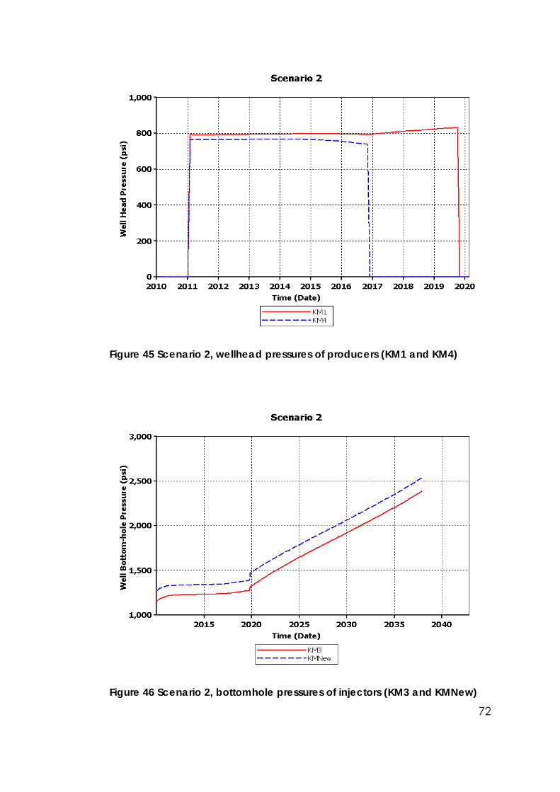
72
Figure 45 Scenario 2, wellhead pressures of producers (KM1 and KM4)
Figure 46 Scenario 2, bottomhole pressures of injectors (KM3 and KMNew)
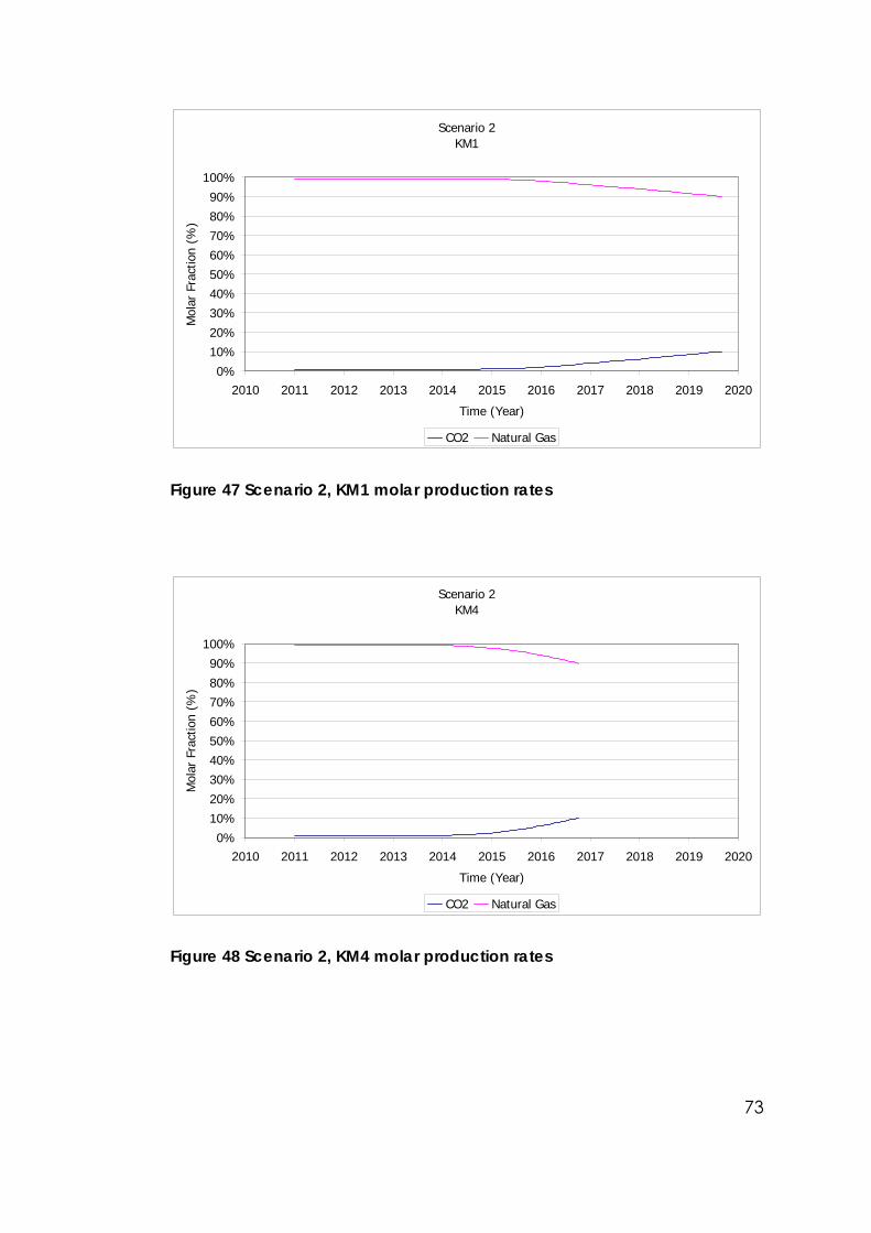
73
Scenario 2KM1
0%
10%20%
30%40%50%60%
70%80%
90%
100%
2010 2011 2012 2013 2014 2015 2016 2017 2018 2019 2020
Time (Year)
Mol
ar F
ract
ion
(%)
CO2 Natural Gas
Figure 47 Scenario 2, KM1 molar production rates
Scenario 2KM4
0%
10%20%
30%40%50%60%
70%80%
90%
100%
2010 2011 2012 2013 2014 2015 2016 2017 2018 2019 2020
Time (Year)
Mol
ar F
ract
ion
(%)
CO2 Natural Gas
Figure 48 Scenario 2, KM4 molar production rates
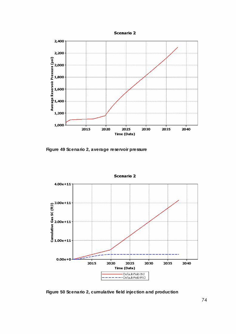
74
Figure 49 Scenario 2, average reservoir pressure
Figure 50 Scenario 2, cumulative field injection and production
75
Scenario 3
Producers required longer time before starting production because their
wellhead pressures could not be maintained if they had been opened
earlier. During 5 years of injection time CO2 propagated far towards the low
permeability regions and this shortened the CO2 breakthrough times in both
of the producers (Figure 51 and Figure 52). KMNew remained in production
about 3.5 years (Figure 53 and Figure 54) and KM3 production time was
about 4.5 years (Figure 55 and Figure 56).
Throughout the production period these wells produced 5472 MMscf and
7912 MMscf natural gas respectively. Total production from the field was
13384 MMscf with a recovery rate of 62.46%.
Less natural gas production lowered CO2 storage capacity of the reservoir.
Maximum amount of CO2 to be stored in the field became 284839 MMscf
for this case (Figure 64).
Table 24 and Table 25 show the numerical results of the scenario. Figure 59
to Figure 63 show constraints that were used in the simulation. CO2
propagation and natural gas movement is displayed in Figure 51 Figure 58.
Placing producers in high permeability region had negative effects in this
scenario. Since higher grid layers could not hold much CO2, CO2
penetrated into lower grid layers easily. This caused a faster front velocity
within lower grid layers. Reaching the lower porosity regions made the front
velocity even faster and CO2 front reached the injector wells in a
considerably shorter time.
CO2 breakthrough occurs once any one of the CO2 containing grid layers
reaches a well grid (Figure 54 and Figure 56). In the case of Kuzey Marmara
this grid layer is the deepest one. If permeability of the grid layers is high CO2
within the grid layers is able to reach faster to the producing well locations
and this causes a significant reduction in CO2 breakthrough times.
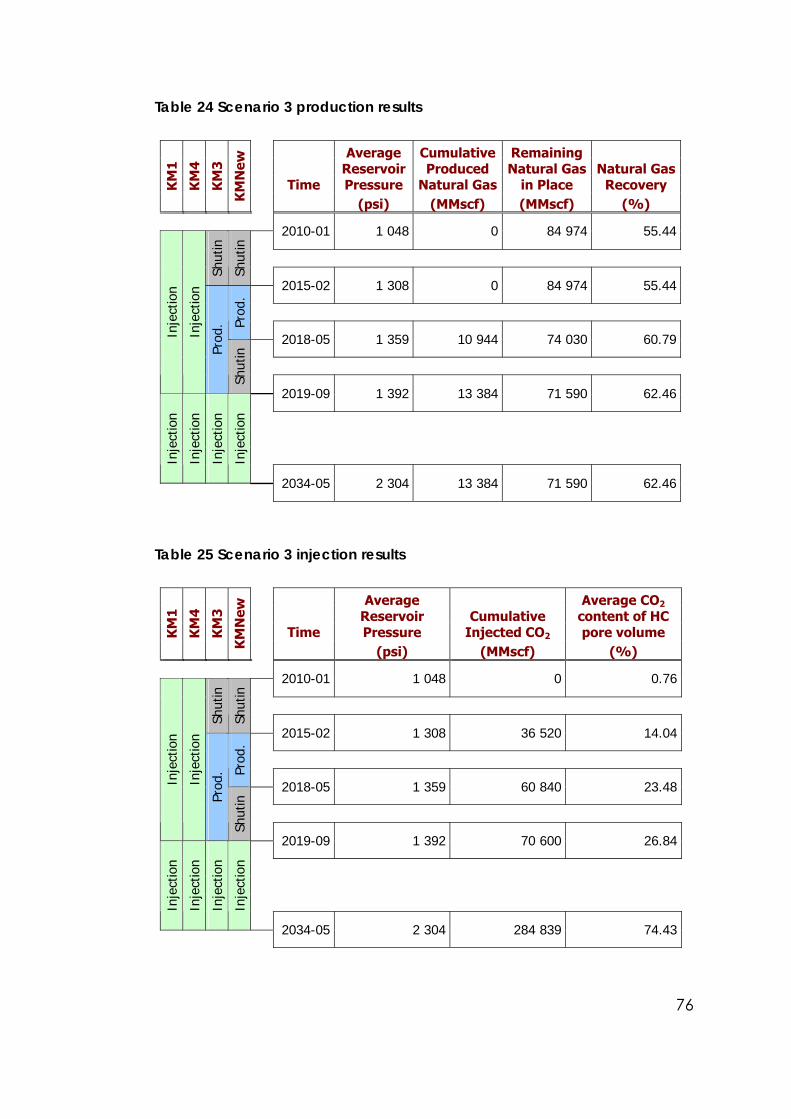
76
Table 24 Scenario 3 production results
Time
Average Reservoir Pressure
Cumulative Produced
Natural Gas
Remaining Natural Gas
in Place Natural Gas
Recovery KM
1
KM
4
KM
3
KM
New
(psi) (MMscf) (MMscf) (%)
2010-01 1 048 0 84 974 55.44
Shut
in
Shut
in
2015-02 1 308 0 84 974 55.44
Prod
.
2018-05 1 359 10 944 74 030 60.79
Inje
ctio
n
Inje
ctio
n
Prod
.
Shut
in
2019-09 1 392 13 384 71 590 62.46
Inje
ctio
n
Inje
ctio
n
Inje
ctio
n
Inje
ctio
n
2034-05 2 304 13 384 71 590 62.46
Table 25 Scenario 3 injection results
Time
Average Reservoir Pressure
Cumulative Injected CO2
Average CO2 content of HC pore volume K
M1
KM
4
KM
3
KM
New
(psi) (MMscf) (%)
2010-01 1 048 0 0.76
Shut
in
Shut
in
2015-02 1 308 36 520 14.04
Prod
.
2018-05 1 359 60 840 23.48
Inje
ctio
n
Inje
ctio
n
Prod
.
Shut
in
2019-09 1 392 70 600 26.84
Inje
ctio
n
Inje
ctio
n
Inje
ctio
n
Inje
ctio
n
2034-05 2 304 284 839 74.43
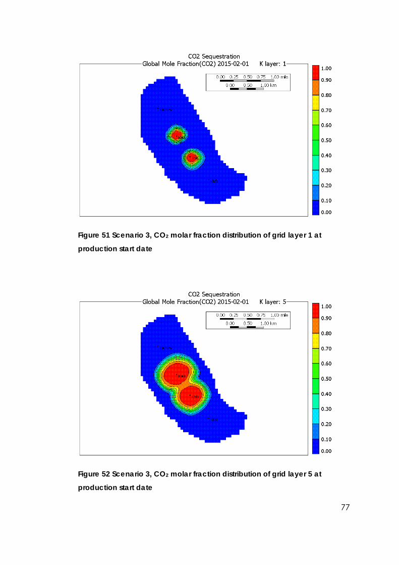
77
Figure 51 Scenario 3, CO2 molar fraction distribution of grid layer 1 at
production start date
Figure 52 Scenario 3, CO2 molar fraction distribution of grid layer 5 at
production start date

78
Figure 53 Scenario 3, CO2 molar fraction distribution of grid layer 1 at
KMNew shutin date
Figure 54 Scenario 3, CO2 molar fraction distribution of grid layer 5 at
KMNew shutin date
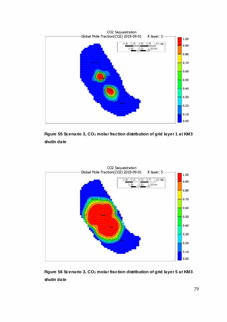
79
Figure 55 Scenario 3, CO2 molar fraction distribution of grid layer 1 at KM3
shutin date
Figure 56 Scenario 3, CO2 molar fraction distribution of grid layer 5 at KM3
shutin date
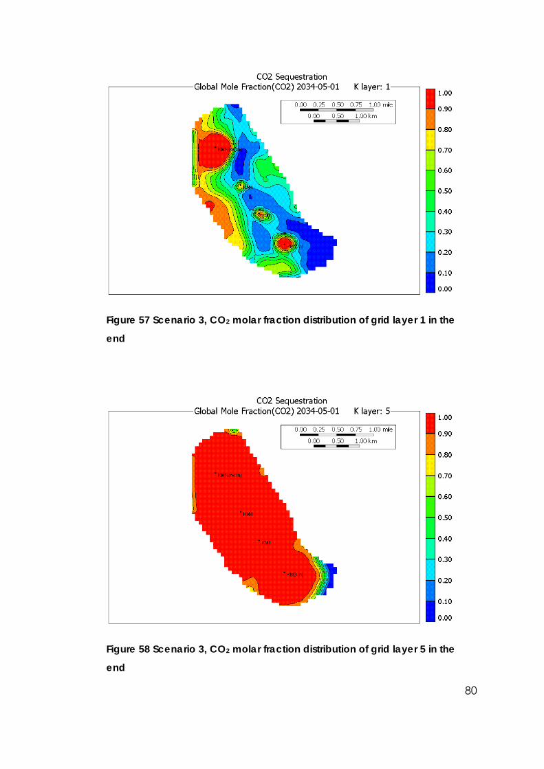
80
Figure 57 Scenario 3, CO2 molar fraction distribution of grid layer 1 in the
end
Figure 58 Scenario 3, CO2 molar fraction distribution of grid layer 5 in the
end
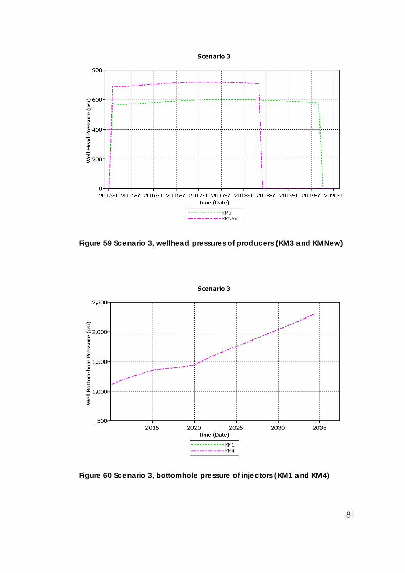
81
Figure 59 Scenario 3, wellhead pressures of producers (KM3 and KMNew)
Figure 60 Scenario 3, bottomhole pressure of injectors (KM1 and KM4)
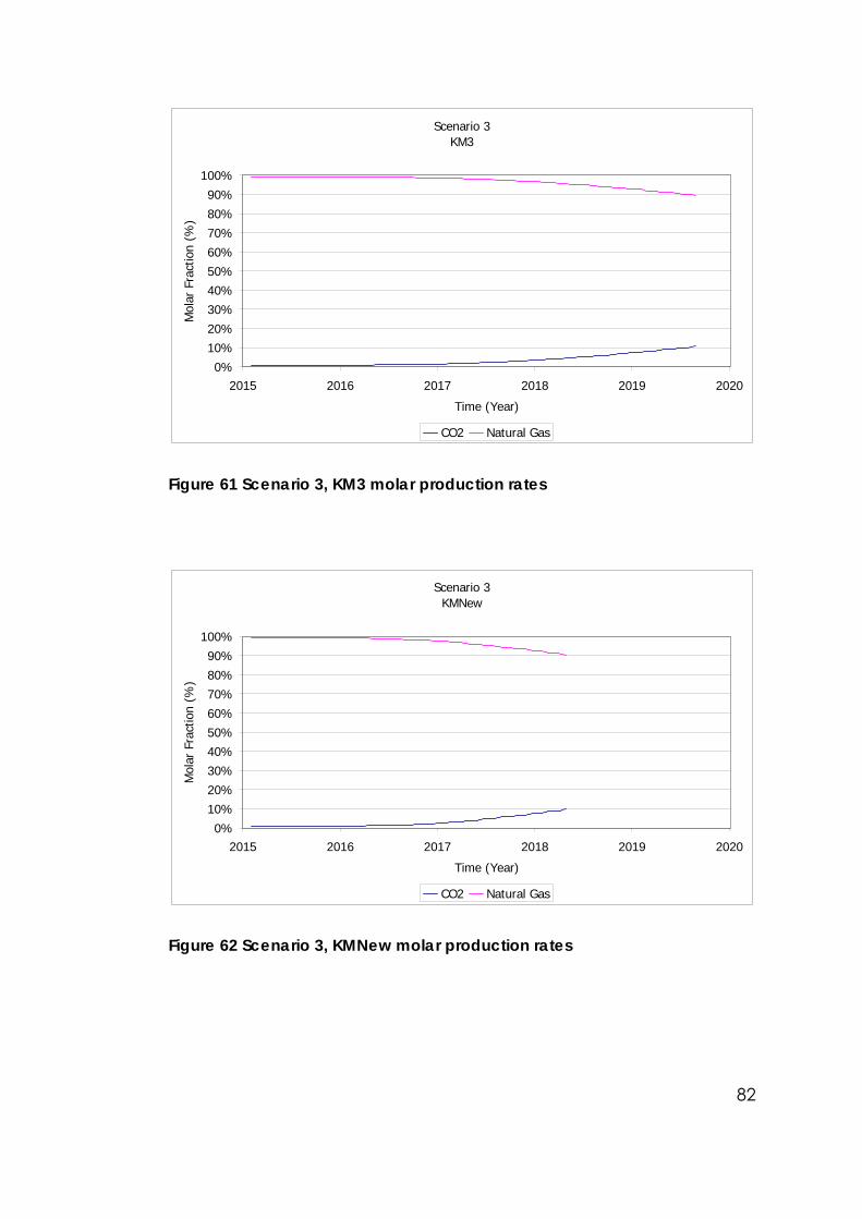
82
Scenario 3KM3
0%
10%20%
30%40%50%60%
70%80%
90%
100%
2015 2016 2017 2018 2019 2020
Time (Year)
Mol
ar F
ract
ion
(%)
CO2 Natural Gas
Figure 61 Scenario 3, KM3 molar production rates
Scenario 3KMNew
0%
10%20%
30%40%50%60%
70%80%
90%
100%
2015 2016 2017 2018 2019 2020
Time (Year)
Mol
ar F
ract
ion
(%)
CO2 Natural Gas
Figure 62 Scenario 3, KMNew molar production rates
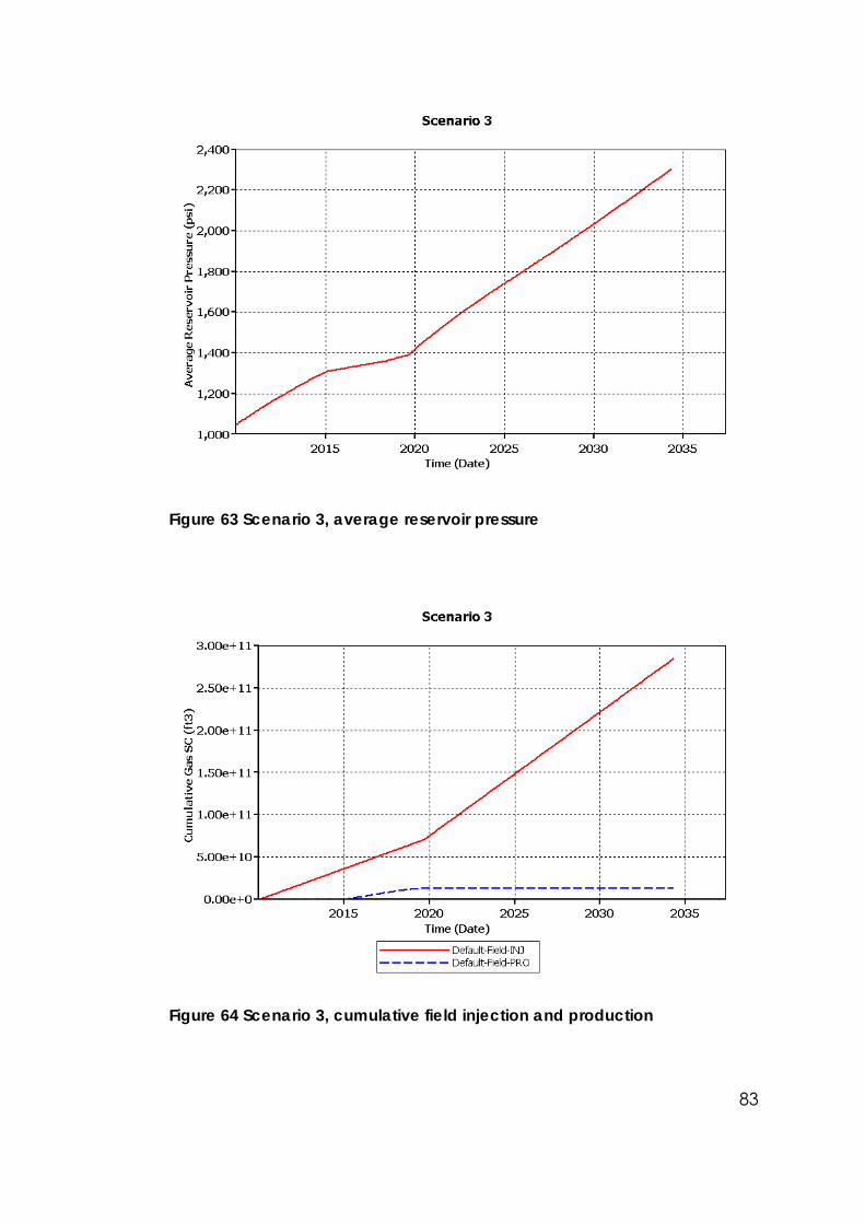
83
Figure 63 Scenario 3, average reservoir pressure
Figure 64 Scenario 3, cumulative field injection and production
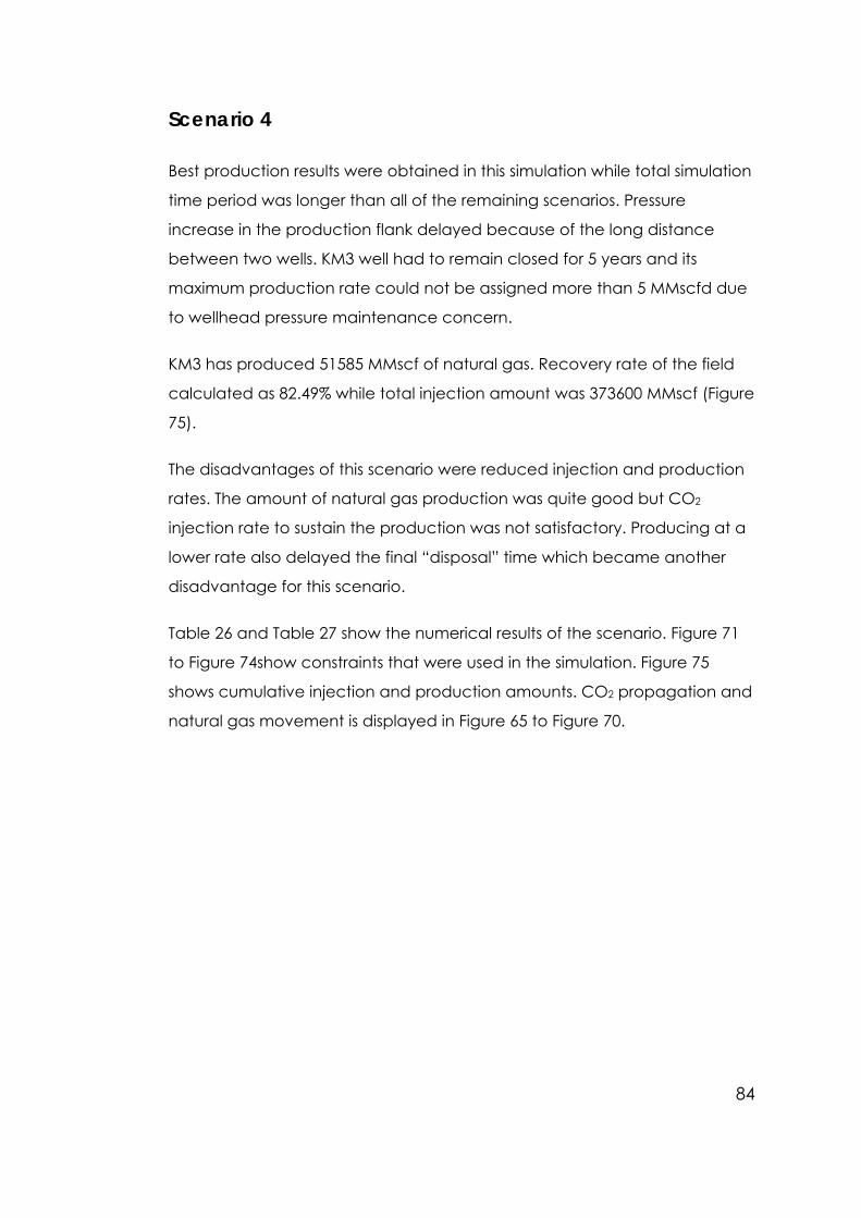
84
Scenario 4
Best production results were obtained in this simulation while total simulation
time period was longer than all of the remaining scenarios. Pressure
increase in the production flank delayed because of the long distance
between two wells. KM3 well had to remain closed for 5 years and its
maximum production rate could not be assigned more than 5 MMscfd due
to wellhead pressure maintenance concern.
KM3 has produced 51585 MMscf of natural gas. Recovery rate of the field
calculated as 82.49% while total injection amount was 373600 MMscf (Figure
75).
The disadvantages of this scenario were reduced injection and production
rates. The amount of natural gas production was quite good but CO2
injection rate to sustain the production was not satisfactory. Producing at a
lower rate also delayed the final “disposal” time which became another
disadvantage for this scenario.
Table 26 and Table 27 show the numerical results of the scenario. Figure 71
to Figure 74show constraints that were used in the simulation. Figure 75
shows cumulative injection and production amounts. CO2 propagation and
natural gas movement is displayed in Figure 65 to Figure 70.
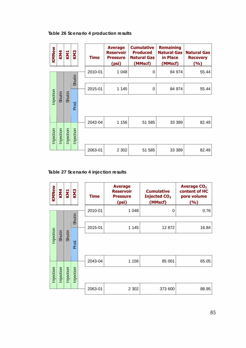
85
Table 26 Scenario 4 production results
Time
Average Reservoir Pressure
Cumulative Produced
Natural Gas
Remaining Natural Gas
in Place Natural Gas
Recovery K
MN
ew
KM
4
KM
1
KM
3
(psi) (MMscf) (MMscf) (%)
2010-01 1 048 0 84 974 55.44
Sh
utin
2015-01 1 145 0 84 974 55.44
Inje
ctio
n
Shut
in
Shut
in
Prod
.
2043-04 1 156 51 585 33 389 82.49
Inje
ctio
n
Inje
ctio
n
Inje
ctio
n
Inje
ctio
n
2063-01 2 302 51 585 33 389 82.49
Table 27 Scenario 4 injection results
Time
Average Reservoir Pressure
Cumulative Injected CO2
Average CO2 content of HC pore volume
KM
New
KM
4
KM
1
KM
3
(psi) (MMscf) (%)
2010-01 1 048 0 0.76
Shut
in
2015-01 1 145 12 872 16.84
Inje
ctio
n
Shut
in
Shut
in
Prod
.
2043-04 1 156 85 001 65.05
Inje
ctio
n
Inje
ctio
n
Inje
ctio
n
Inje
ctio
n
2063-01 2 302 373 600 88.95
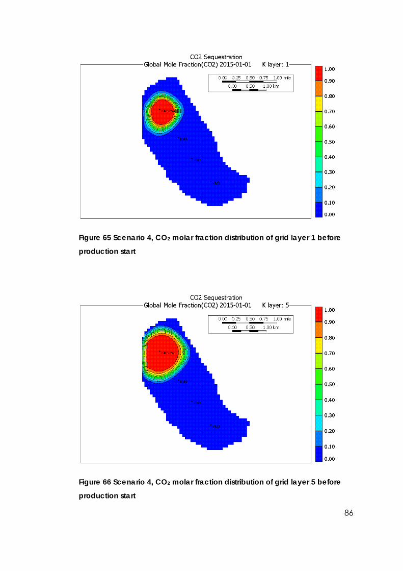
86
Figure 65 Scenario 4, CO2 molar fraction distribution of grid layer 1 before
production start
Figure 66 Scenario 4, CO2 molar fraction distribution of grid layer 5 before
production start
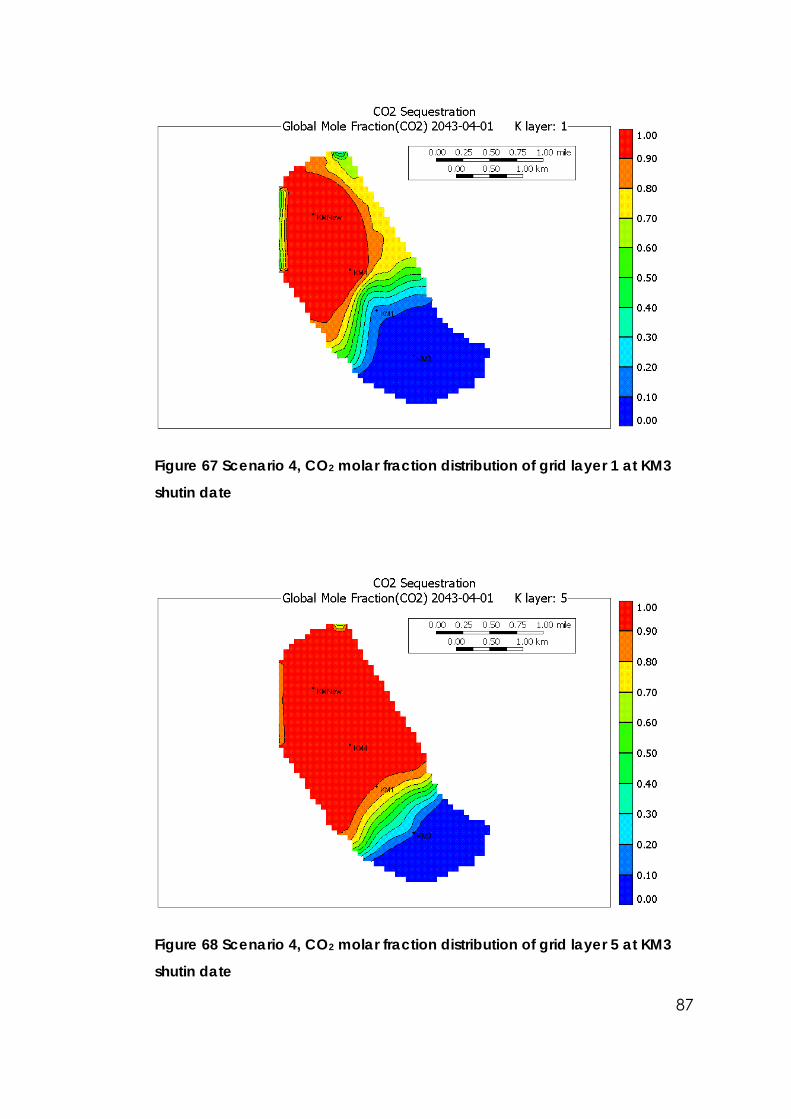
87
Figure 67 Scenario 4, CO2 molar fraction distribution of grid layer 1 at KM3
shutin date
Figure 68 Scenario 4, CO2 molar fraction distribution of grid layer 5 at KM3
shutin date
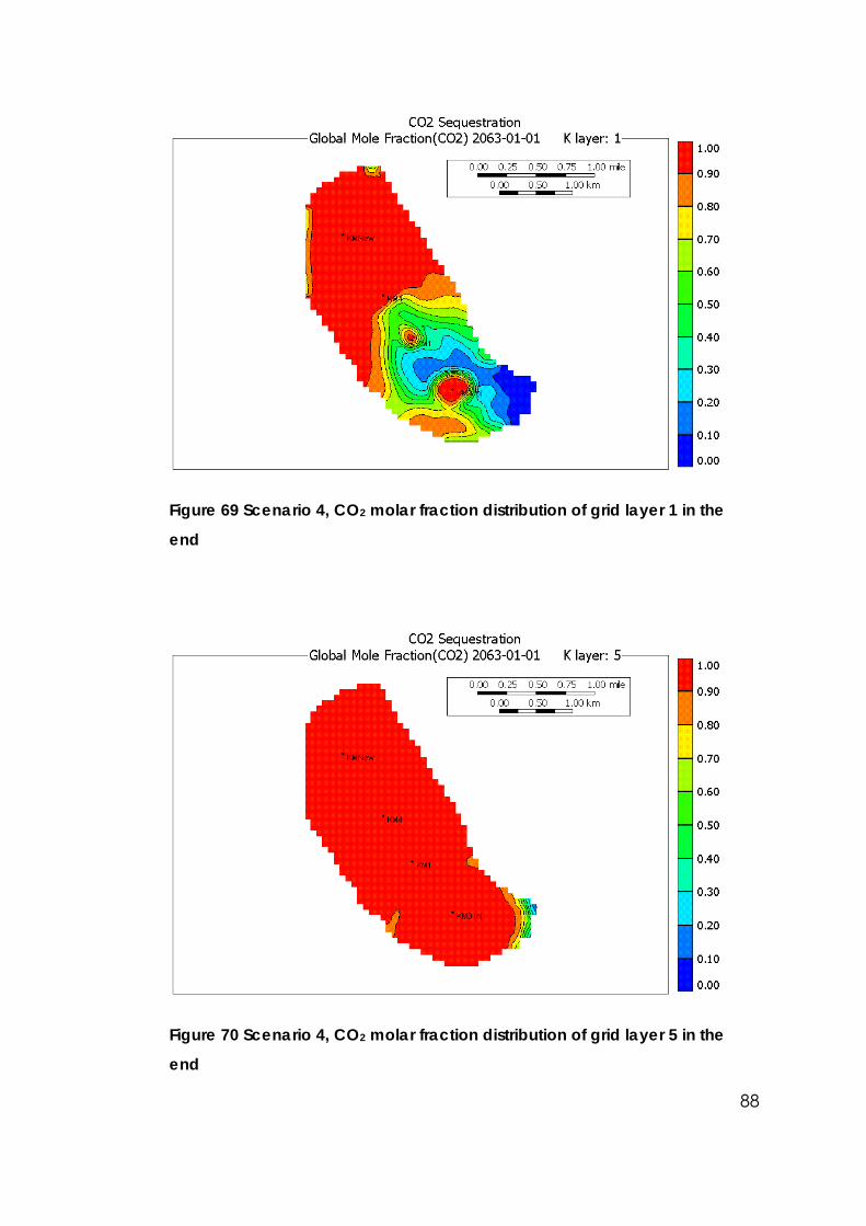
88
Figure 69 Scenario 4, CO2 molar fraction distribution of grid layer 1 in the
end
Figure 70 Scenario 4, CO2 molar fraction distribution of grid layer 5 in the
end
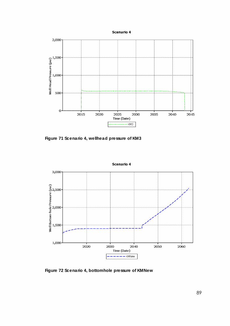
89
Figure 71 Scenario 4, wellhead pressure of KM3
Figure 72 Scenario 4, bottomhole pressure of KMNew
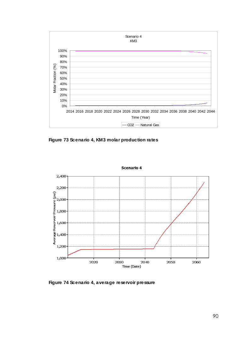
90
Scenario 4KM3
0%
10%20%
30%40%50%60%
70%80%
90%
100%
2014 2016 2018 2020 2022 2024 2026 2028 2030 2032 2034 2036 2038 2040 2042 2044
Time (Year)
Mol
ar F
ract
ion
(%)
CO2 Natural Gas
Figure 73 Scenario 4, KM3 molar production rates
Figure 74 Scenario 4, average reservoir pressure
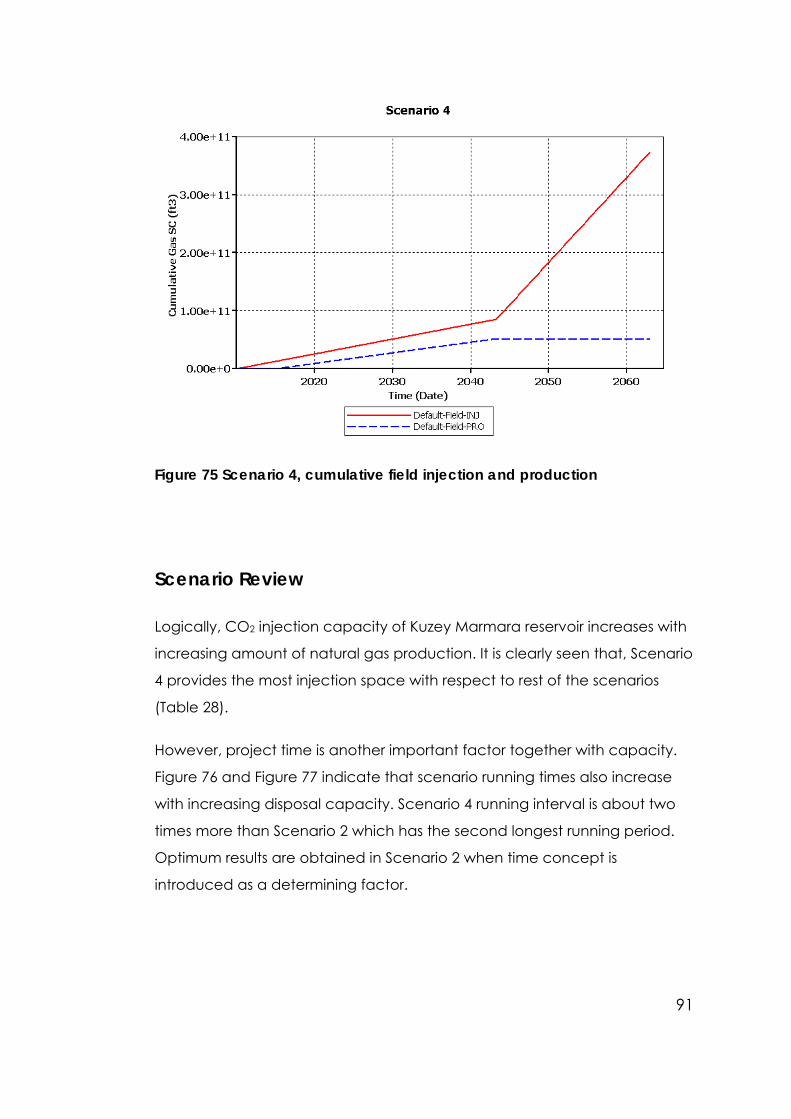
91
Figure 75 Scenario 4, cumulative field injection and production
Scenario Review
Logically, CO2 injection capacity of Kuzey Marmara reservoir increases with
increasing amount of natural gas production. It is clearly seen that, Scenario
4 provides the most injection space with respect to rest of the scenarios
(Table 28).
However, project time is another important factor together with capacity.
Figure 76 and Figure 77 indicate that scenario running times also increase
with increasing disposal capacity. Scenario 4 running interval is about two
times more than Scenario 2 which has the second longest running period.
Optimum results are obtained in Scenario 2 when time concept is
introduced as a determining factor.
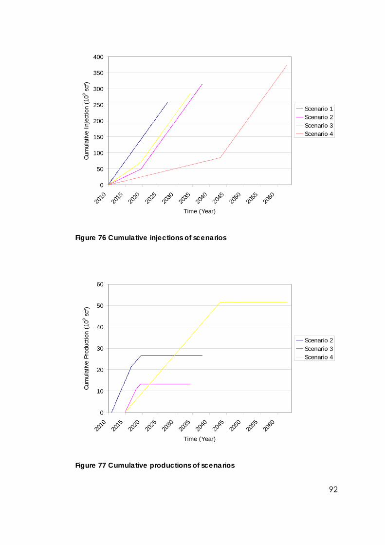
92
0
50
100
150
200
250
300
350
400
2010
2015
2020
2025
2030
2035
2040
2045
2050
2055
2060
Time (Year)
Cum
ulat
ive
Inje
ctio
n (1
09 scf
)
Scenario 1Scenario 2Scenario 3Scenario 4
Figure 76 Cumulative injections of scenarios
0
10
20
30
40
50
60
2010
2015
2020
2025
2030
2035
2040
2045
2050
2055
2060
Time (Year)
Cum
ulat
ive
Prod
uctio
n (1
09 scf
)
Scenario 2Scenario 3Scenario 4
Figure 77 Cumulative productions of scenarios

93
Table 28 Scenario results overview
Scenario Length
Cumulative Injection
Cumulative Production
∆Injection Si – S1
(Years) (MMscf) (MMscf) (MMscf)
Scenario 1 17.7 258 078 0 0
Scenario 2 27.9 315 279 26 630 57 201
Scenario 3 24.3 284 839 13 384 26 761
Scenario 4 53.0 373 600 51 585 115 522
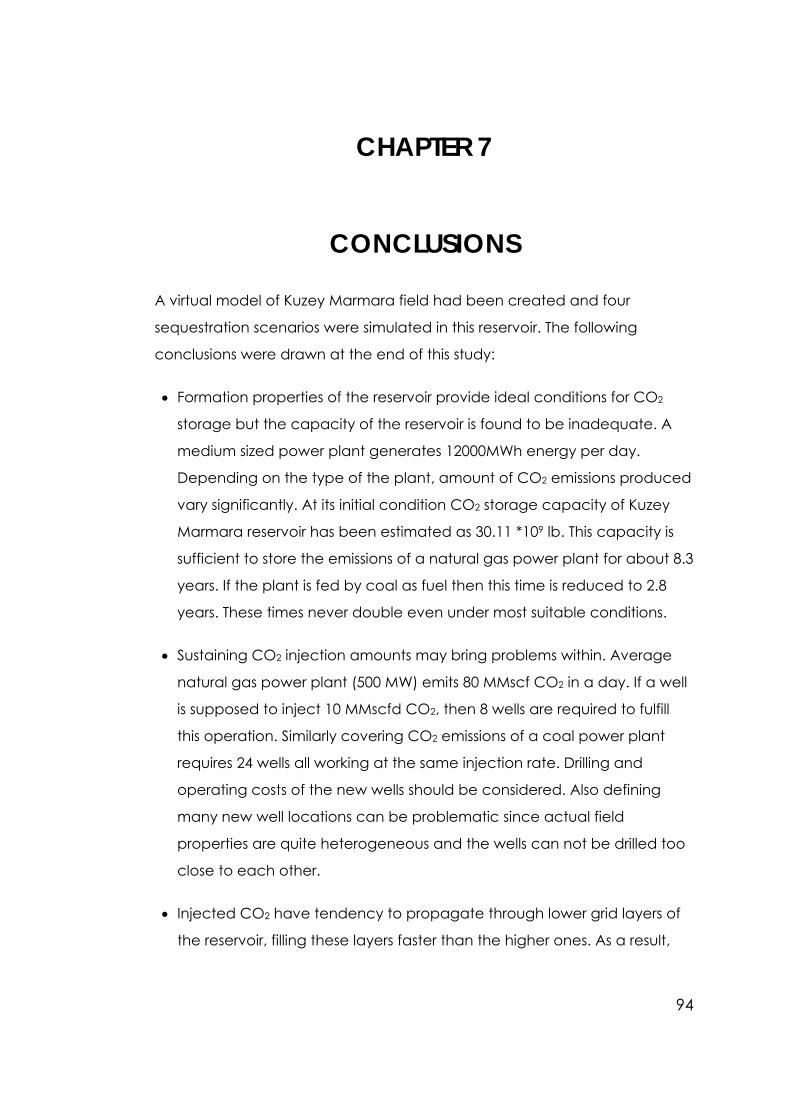
94
CHAPTER 7
CONCLUSIONS
A virtual model of Kuzey Marmara field had been created and four
sequestration scenarios were simulated in this reservoir. The following
conclusions were drawn at the end of this study:
• Formation properties of the reservoir provide ideal conditions for CO2
storage but the capacity of the reservoir is found to be inadequate. A
medium sized power plant generates 12000MWh energy per day.
Depending on the type of the plant, amount of CO2 emissions produced
vary significantly. At its initial condition CO2 storage capacity of Kuzey
Marmara reservoir has been estimated as 30.11 *109 lb. This capacity is
sufficient to store the emissions of a natural gas power plant for about 8.3
years. If the plant is fed by coal as fuel then this time is reduced to 2.8
years. These times never double even under most suitable conditions.
• Sustaining CO2 injection amounts may bring problems within. Average
natural gas power plant (500 MW) emits 80 MMscf CO2 in a day. If a well
is supposed to inject 10 MMscfd CO2, then 8 wells are required to fulfill
this operation. Similarly covering CO2 emissions of a coal power plant
requires 24 wells all working at the same injection rate. Drilling and
operating costs of the new wells should be considered. Also defining
many new well locations can be problematic since actual field
properties are quite heterogeneous and the wells can not be drilled too
close to each other.
• Injected CO2 have tendency to propagate through lower grid layers of
the reservoir, filling these layers faster than the higher ones. As a result,

95
natural gas was moved towards the upper grid layers and away from
the injection wells.
• Injecting CO2 from high porosity regions demonstrates the best
conditions for sequestration. High porosity limits front velocity while
providing much space to store injected fluid.
• Permeability is another fact that effects fluid propagation. Permeability
variation effects direction of propagation rather than propagation
velocity. Downward movement of CO2 becomes easier in high
permeability regions. At the same time front velocity in lower regions
decreases.
Finally, CO2 injection can be applied to increase natural gas recovery of
Kuzey Marmara field but sequestering high rate CO2 emissions is found out
to be inappropriate.
96
REFERENCES
1. Karaoğuz O., Kalfa Ü., Uygur E., Korucu Ö., Alper Z., Southwood D.:
“Reservoir Study for Kuzey Marmara Underground Gas Storage
Project”, Proceedings – 14th International Petroleum and Natural Gas
Congress and Exhibition of Turkey, Ankara, Turkey, 2003.
2. Bakiler C. S., Yilmaz M.: “Underground Storage of Natural gas in Kuzey
Marmara and Değirmenköy Fields”, International Symposium on
Underground Storage of Natural Gas ’99, Proceedings, Ankara,
Turkey, June, 1999.
3. Çınar G., Vrana L.: “The Development of North Marmara Offshore
Gas Field”, 9th Petroleum Congress and Exhibition of Türkiye,
Proceedings, Ankara, Turkey, February 1992.
4. Bakiler C. S., İşsever K., Atalay T., Gültekin C.: “Development of the
Kuzey Marmara Natural Gas Field, the First Offshore Field in Turkey”,
Proceedings – 12th International Petroleum Congress of Turkey,
Ankara, Turkey 1998.
5. Satman A., Karaalioğlu H., Kızılöğren H.: “Possibilities of Underground
Storage in Turkey”, 11th Petroleum Congress and Exhibition of Turkey,
Ankara, Turkey, April 1996.
6. Ulaş T., Cengiz M.: “North Marmara Development Drilling”,
“Possibilities of Underground Storage in Turkey”, 11th Petroleum
Congress and Exhibition of Turkey, Ankara, Turkey, April 1996.
7. United Nations Environment Programme and the Climate Change
Secretariat (UNFCCC): “Climate Change Information Kit”, July 2002.
8. Natural Resources Defense Council (NRDC), Public Service Enterprise
Group (PSEG), Corporate Climate Accountability Project of Coalition
97
for Environmentally Responsible Economies (CERES): “Benchmarking
Air Emissions of the 100 Largest Electric Generation Owners in the U.S.
– 2000”, Second Edition, March 2002.
9. Intergovernmental Panel on Climate Change (IPCC): ”Climate
Change 2001: The Scientific Basis”, Cambridge University Press, 2001.
10. International Energy Agency (IEA): “World Energy Outlook 2002”,
Second edition, November 2002.
11. International Energy Agency (IEA): “CO2 Capture at Power Stations
and Other Major Point Sources”, 2002.
12. Gambini M., Velini M.: “CO2 Emission Abatement from Fossil Fuel
Power Plants by Exhaust Gas Treatment”, IJPGC2000-15056
Proceedings of 2000 International Joint Power Generation
Conference, Miami Beach Florida, July 2000.
13. Dortmundt D., Doshi K.: “Recent Developments in CO2 Removal
Membrane Technology”, 1999.
14. International Energy Agency (IEA): “CO2 Capture and Storage in
Geological Formations”, 2002.
15. Oldenburg C., D. H. -S. Law, Y. Le Gallo, S. P. White: “Mixing of CO2
and CH4 in Gas Reservoirs: Code Comparison Studies", University of
California, Paper LBNL 49763, 2002.
16. Tureyen Ö. İ., Karaalioglu H., Satman S.: “Effect of Wellbore
Conditions on the Performance of Underground Gas Storage
Reservoirs”, Istanbul Technical University, SPE 59737, April 2000
17. Pidwirny M., “Fundementals of Physical Georgaphy”,
http://www.physicalgeography.net/fundamentals/7a.html, April
2004, last accessed date September 2005.

98
18. Golden Software. Inc., http://www.goldensoftware.com, 2004, last
accessed date September 2005.
19. Computer Modeling Group (CMG) Ltd., http://www.cmgroup.com,
August 2005, last accessed date September 2005.
20. Computer Modeling Group (CMG): “GEM, Advanced Compositional
Reservoir Simulator, Version 2004 User’s Guide”, 2004.
21. Computer Modeling Group (CMG): “WinProp, Phase Property
Program, Version 2004 User’s Guide”, 2004.
22. Öztürk B.: “Simulation of Depleted Gas Reservoir for Underground
Storage”, M. Sc. Department of Petroleum and Natural Gas
Engineering, Middle East Technical University, Ankara, Turkey,
December 2004.
23. Hopkins W. G.: “A New View of Statistics”,
http://www.sportsci.org/resource/stats/rmse.html, April 1997, last
accessed date September 2005.
24. Schlumberger: “i-Handbook”,
http://www.oilfield.slb.com/content/services/resources/software/iha
ndbook.asp, September 2004, last accessed date September 2005.
25. Daxesoft Ltd.: “Engineering Software for Fluid Flow and Pressure Drop
Calculations”,
http://www.pipeflow.co.uk/public/control.php?_path=/497/503/510,
2005, last accessed date September 2005.
26. Blasing T. J., Jones S.: “Current Greenhouse Gas Concentrations”,
http://cdiac.esd.ornl.gov/pns/current_ghg.html, February 2005, last
accessed date September 2005.
99
27. Globalis: “Turkey: Carbon dioxide emissions”,
http://globalis.gvu.unu.edu/indicator_detail.cfm?Country=TR&Indica
torID=48, 2002, last accessed date September 2005.
28. Gümüş A., Top A., Eren Ş., Cerrah M., Önem K., Ülgün F. S.: “ERD
Application for Kuzey Marmara Underground Gas Storage Wells”, 15th
International Petroleum and Natural Gas Congress and Exhibition of
Turkey, 11-13 May 2005, Bilkent Hotel, Ankara, Turkey.
29. Abravcı S., Titrek A., Karaman T., Uysal S.: “Turkish Petroleum
Corporation Kuzey Marmara and Değirmenköy Underground Gas
Storages”, 15th International Petroleum and Natural Gas Congress
and Exhibition of Turkey, 11-13 May 2005, Bilkent Hotel, Ankara,
Turkey.
30. Mustafa Y., Abravcı S., Saraçoğlu Ö: “Development of an
Underground Gas Storage: Kuzey Marmara Field”, 15th International
Petroleum and Natural Gas Congress and Exhibition of Turkey, 11-13
May 2005, Bilkent Hotel, Ankara, Turkey.
31. Başbuğ B.: “Modeling of Carbon Dioxide Sequestration in a Deep
Saline Aquifer”, M. Sc. Department of Petroleum and Natural Gas
Engineering, Middle East Technical University, Ankara, Turkey, July
2005.
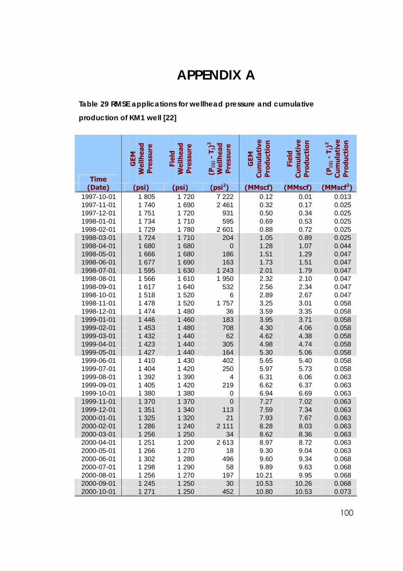
100
APPENDIX A
Table 29 RMSE applications for wellhead pressure and cumulative
production of KM1 well [22]
Time
GEM
W
ellh
ead
Pre
ssu
re
Fiel
d W
ellh
ead
Pre
ssu
re
(P(i
j) -
Tj)
2
Wel
lhea
d P
ress
ure
GEM
C
um
ula
tive
P
rodu
ctio
n
Fiel
d C
um
ula
tive
P
rodu
ctio
n
(P(i
j) -
Tj)
2
Cu
mu
lati
ve
Pro
duct
ion
(Date) (psi) (psi) (psi2) (MMscf) (MMscf) (MMscf2) 1997-10-01 1 805 1 720 7 222 0.12 0.01 0.013 1997-11-01 1 740 1 690 2 461 0.32 0.17 0.025 1997-12-01 1 751 1 720 931 0.50 0.34 0.025 1998-01-01 1 734 1 710 595 0.69 0.53 0.025 1998-02-01 1 729 1 780 2 601 0.88 0.72 0.025 1998-03-01 1 724 1 710 204 1.05 0.89 0.025 1998-04-01 1 680 1 680 0 1.28 1.07 0.044 1998-05-01 1 666 1 680 186 1.51 1.29 0.047 1998-06-01 1 677 1 690 163 1.73 1.51 0.047 1998-07-01 1 595 1 630 1 243 2.01 1.79 0.047 1998-08-01 1 566 1 610 1 950 2.32 2.10 0.047 1998-09-01 1 617 1 640 532 2.56 2.34 0.047 1998-10-01 1 518 1 520 6 2.89 2.67 0.047 1998-11-01 1 478 1 520 1 757 3.25 3.01 0.058 1998-12-01 1 474 1 480 36 3.59 3.35 0.058 1999-01-01 1 446 1 460 183 3.95 3.71 0.058 1999-02-01 1 453 1 480 708 4.30 4.06 0.058 1999-03-01 1 432 1 440 62 4.62 4.38 0.058 1999-04-01 1 423 1 440 305 4.98 4.74 0.058 1999-05-01 1 427 1 440 164 5.30 5.06 0.058 1999-06-01 1 410 1 430 402 5.65 5.40 0.058 1999-07-01 1 404 1 420 250 5.97 5.73 0.058 1999-08-01 1 392 1 390 4 6.31 6.06 0.063 1999-09-01 1 405 1 420 219 6.62 6.37 0.063 1999-10-01 1 380 1 380 0 6.94 6.69 0.063 1999-11-01 1 370 1 370 0 7.27 7.02 0.063 1999-12-01 1 351 1 340 113 7.59 7.34 0.063 2000-01-01 1 325 1 320 21 7.93 7.67 0.063 2000-02-01 1 286 1 240 2 111 8.28 8.03 0.063 2000-03-01 1 256 1 250 34 8.62 8.36 0.063 2000-04-01 1 251 1 200 2 613 8.97 8.72 0.063 2000-05-01 1 266 1 270 18 9.30 9.04 0.063 2000-06-01 1 302 1 280 496 9.60 9.34 0.068 2000-07-01 1 298 1 290 58 9.89 9.63 0.068 2000-08-01 1 256 1 270 197 10.21 9.95 0.068 2000-09-01 1 245 1 250 30 10.53 10.26 0.068 2000-10-01 1 271 1 250 452 10.80 10.53 0.073
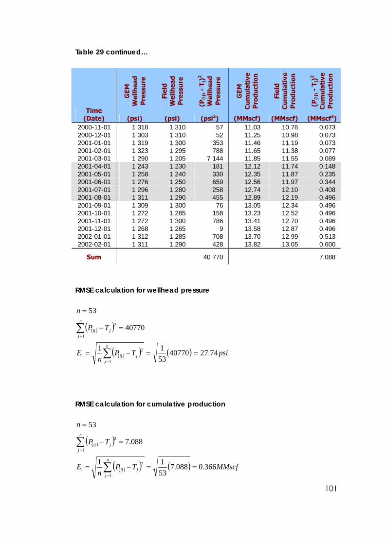
101
Table 29 continued…
Time
GEM
W
ellh
ead
Pre
ssu
re
Fiel
d W
ellh
ead
Pre
ssu
re
(P(i
j) -
Tj)
2
Wel
lhea
d P
ress
ure
GEM
C
um
ula
tive
P
rodu
ctio
n
Fiel
d C
um
ula
tive
P
rodu
ctio
n
(P(i
j) -
Tj)
2
Cu
mu
lati
ve
Pro
duct
ion
(Date) (psi) (psi) (psi2) (MMscf) (MMscf) (MMscf2) 2000-11-01 1 318 1 310 57 11.03 10.76 0.073 2000-12-01 1 303 1 310 52 11.25 10.98 0.073 2001-01-01 1 319 1 300 353 11.46 11.19 0.073 2001-02-01 1 323 1 295 788 11.65 11.38 0.077 2001-03-01 1 290 1 205 7 144 11.85 11.55 0.089 2001-04-01 1 243 1 230 181 12.12 11.74 0.148 2001-05-01 1 258 1 240 330 12.35 11.87 0.235 2001-06-01 1 276 1 250 659 12.56 11.97 0.344 2001-07-01 1 296 1 280 258 12.74 12.10 0.408 2001-08-01 1 311 1 290 455 12.89 12.19 0.496 2001-09-01 1 309 1 300 76 13.05 12.34 0.496 2001-10-01 1 272 1 285 158 13.23 12.52 0.496 2001-11-01 1 272 1 300 786 13.41 12.70 0.496 2001-12-01 1 268 1 265 9 13.58 12.87 0.496 2002-01-01 1 312 1 285 708 13.70 12.99 0.513 2002-02-01 1 311 1 290 428 13.82 13.05 0.600
Sum 40 770 7.088
RMSE calculation for wellhead pressure
( )( )
( )( ) ( ) psiTPn
E
TP
n
n
jjiji
n
jjij
74.27407705311
40770
53
1
2
1
2
==−=
=−
=
∑
∑
=
=
RMSE calculation for cumulative production
( )( )
( )( ) ( ) MMscfTPn
E
TP
n
n
jjiji
n
jjij
366.0088.75311
088.7
53
1
2
1
2
==−=
=−
=
∑
∑
=
=
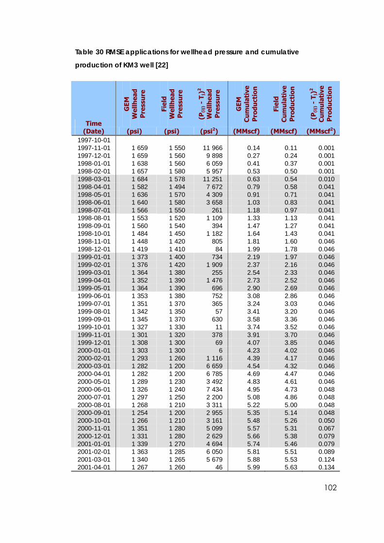
102
Table 30 RMSE applications for wellhead pressure and cumulative
production of KM3 well [22]
Time G
EM
Wel
lhea
d P
ress
ure
Fiel
d W
ellh
ead
Pre
ssu
re
(P(i
j) -
Tj)
2
Wel
lhea
d P
ress
ure
GEM
C
um
ula
tive
P
rodu
ctio
n
Fiel
d C
um
ula
tive
P
rodu
ctio
n
(P(i
j) -
Tj)
2
Cu
mu
lati
ve
Pro
duct
ion
(Date) (psi) (psi) (psi2) (MMscf) (MMscf) (MMscf2) 1997-10-01 1997-11-01 1 659 1 550 11 966 0.14 0.11 0.001 1997-12-01 1 659 1 560 9 898 0.27 0.24 0.001 1998-01-01 1 638 1 560 6 059 0.41 0.37 0.001 1998-02-01 1 657 1 580 5 957 0.53 0.50 0.001 1998-03-01 1 684 1 578 11 251 0.63 0.54 0.010 1998-04-01 1 582 1 494 7 672 0.79 0.58 0.041 1998-05-01 1 636 1 570 4 309 0.91 0.71 0.041 1998-06-01 1 640 1 580 3 658 1.03 0.83 0.041 1998-07-01 1 566 1 550 261 1.18 0.97 0.041 1998-08-01 1 553 1 520 1 109 1.33 1.13 0.041 1998-09-01 1 560 1 540 394 1.47 1.27 0.041 1998-10-01 1 484 1 450 1 182 1.64 1.43 0.041 1998-11-01 1 448 1 420 805 1.81 1.60 0.046 1998-12-01 1 419 1 410 84 1.99 1.78 0.046 1999-01-01 1 373 1 400 734 2.19 1.97 0.046 1999-02-01 1 376 1 420 1 909 2.37 2.16 0.046 1999-03-01 1 364 1 380 255 2.54 2.33 0.046 1999-04-01 1 352 1 390 1 476 2.73 2.52 0.046 1999-05-01 1 364 1 390 696 2.90 2.69 0.046 1999-06-01 1 353 1 380 752 3.08 2.86 0.046 1999-07-01 1 351 1 370 365 3.24 3.03 0.046 1999-08-01 1 342 1 350 57 3.41 3.20 0.046 1999-09-01 1 345 1 370 630 3.58 3.36 0.046 1999-10-01 1 327 1 330 11 3.74 3.52 0.046 1999-11-01 1 301 1 320 378 3.91 3.70 0.046 1999-12-01 1 308 1 300 69 4.07 3.85 0.046 2000-01-01 1 303 1 300 6 4.23 4.02 0.046 2000-02-01 1 293 1 260 1 116 4.39 4.17 0.046 2000-03-01 1 282 1 200 6 659 4.54 4.32 0.046 2000-04-01 1 282 1 200 6 785 4.69 4.47 0.046 2000-05-01 1 289 1 230 3 492 4.83 4.61 0.046 2000-06-01 1 326 1 240 7 434 4.95 4.73 0.048 2000-07-01 1 297 1 250 2 200 5.08 4.86 0.048 2000-08-01 1 268 1 210 3 311 5.22 5.00 0.048 2000-09-01 1 254 1 200 2 955 5.35 5.14 0.048 2000-10-01 1 266 1 210 3 161 5.48 5.26 0.050 2000-11-01 1 351 1 280 5 099 5.57 5.31 0.067 2000-12-01 1 331 1 280 2 629 5.66 5.38 0.079 2001-01-01 1 339 1 270 4 694 5.74 5.46 0.079 2001-02-01 1 363 1 285 6 050 5.81 5.51 0.089 2001-03-01 1 340 1 265 5 679 5.88 5.53 0.124 2001-04-01 1 267 1 260 46 5.99 5.63 0.134

103
Table 30 continued…
Time
GEM
W
ellh
ead
Pre
ssu
re
Fiel
d W
ellh
ead
Pre
ssu
re
(P(i
j) -
Tj)
2
Wel
lhea
d P
ress
ure
GEM
C
um
ula
tive
P
rodu
ctio
n
Fiel
d C
um
ula
tive
P
rodu
ctio
n
(P(i
j) -
Tj)
2
Cu
mu
lati
ve
Pro
duct
ion
(Date) (psi) (psi) (psi2) (MMscf) (MMscf) (MMscf2) 2001-05-01 1 286 1 220 4 335 6.08 5.72 0.134 2001-06-01 1 243 1 175 4 672 6.19 5.77 0.182 2001-07-01 1 274 1 250 573 6.28 5.83 0.205 2001-08-01 1 280 1 240 1 612 6.37 5.87 0.251 2001-09-01 1 301 1 250 2 603 6.45 5.90 0.302 2001-10-01 1 284 1 250 1 148 6.53 5.98 0.302 2001-11-01 1 253 1 230 510 6.62 6.03 0.342 2001-12-01 1 286 1 220 4 393 6.69 6.07 0.382 2002-01-01 1 289 1 220 4 782 6.76 6.13 0.387 2002-01-01 1 263 1 210 2 856 6.83 6.17 0.436
Sum 160 733 4.914
RMSE calculation for wellhead pressure
( )( )
( )( ) ( ) psiTPn
E
TP
n
n
jjiji
n
jjij
60.551607335211
160733
52
1
2
1
2
==−=
=−
=
∑
∑
=
=
RMSE calculation for cumulative production
( )( )
( )( ) ( ) MMscfTPn
E
TP
n
n
jjiji
n
jjij
307.0914.45211
914.4
52
1
2
1
2
==−=
=−
=
∑
∑
=
=
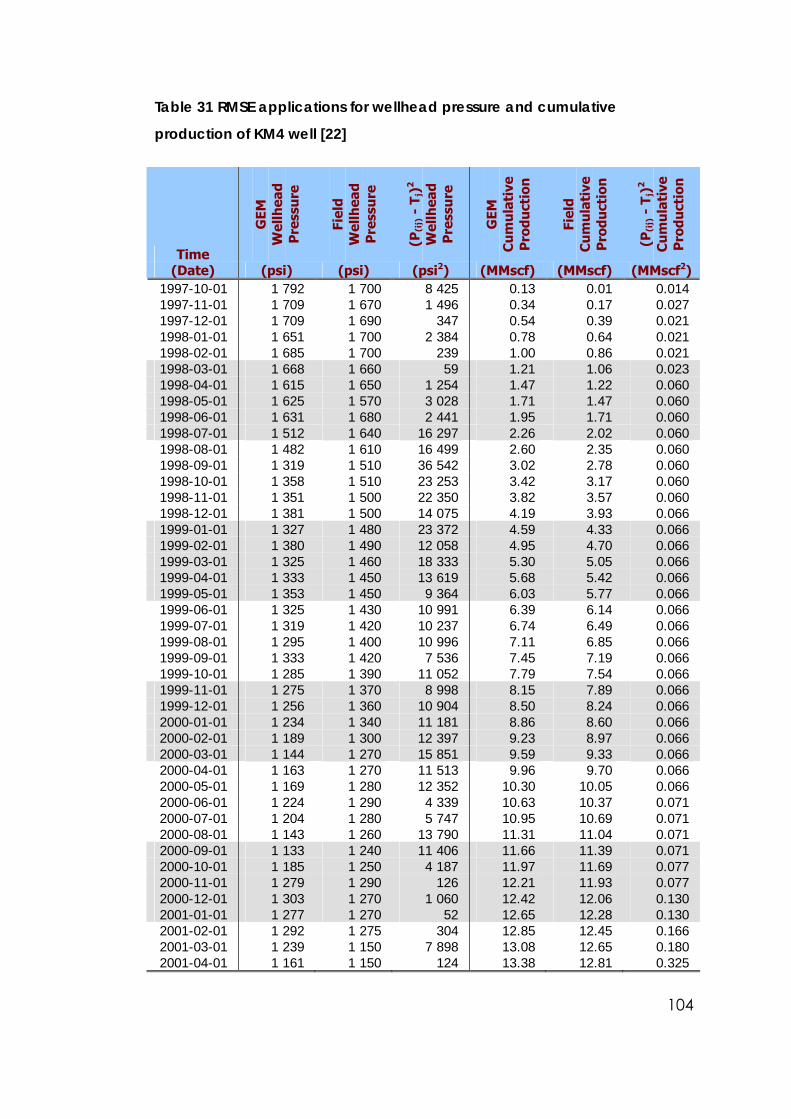
104
Table 31 RMSE applications for wellhead pressure and cumulative
production of KM4 well [22]
Time G
EM
Wel
lhea
d P
ress
ure
Fiel
d W
ellh
ead
Pre
ssu
re
(P(i
j) -
Tj)
2
Wel
lhea
d P
ress
ure
GEM
C
um
ula
tive
P
rodu
ctio
n
Fiel
d C
um
ula
tive
P
rodu
ctio
n
(P(i
j) -
Tj)
2
Cu
mu
lati
ve
Pro
duct
ion
(Date) (psi) (psi) (psi2) (MMscf) (MMscf) (MMscf2) 1997-10-01 1 792 1 700 8 425 0.13 0.01 0.014 1997-11-01 1 709 1 670 1 496 0.34 0.17 0.027 1997-12-01 1 709 1 690 347 0.54 0.39 0.021 1998-01-01 1 651 1 700 2 384 0.78 0.64 0.021 1998-02-01 1 685 1 700 239 1.00 0.86 0.021 1998-03-01 1 668 1 660 59 1.21 1.06 0.023 1998-04-01 1 615 1 650 1 254 1.47 1.22 0.060 1998-05-01 1 625 1 570 3 028 1.71 1.47 0.060 1998-06-01 1 631 1 680 2 441 1.95 1.71 0.060 1998-07-01 1 512 1 640 16 297 2.26 2.02 0.060 1998-08-01 1 482 1 610 16 499 2.60 2.35 0.060 1998-09-01 1 319 1 510 36 542 3.02 2.78 0.060 1998-10-01 1 358 1 510 23 253 3.42 3.17 0.060 1998-11-01 1 351 1 500 22 350 3.82 3.57 0.060 1998-12-01 1 381 1 500 14 075 4.19 3.93 0.066 1999-01-01 1 327 1 480 23 372 4.59 4.33 0.066 1999-02-01 1 380 1 490 12 058 4.95 4.70 0.066 1999-03-01 1 325 1 460 18 333 5.30 5.05 0.066 1999-04-01 1 333 1 450 13 619 5.68 5.42 0.066 1999-05-01 1 353 1 450 9 364 6.03 5.77 0.066 1999-06-01 1 325 1 430 10 991 6.39 6.14 0.066 1999-07-01 1 319 1 420 10 237 6.74 6.49 0.066 1999-08-01 1 295 1 400 10 996 7.11 6.85 0.066 1999-09-01 1 333 1 420 7 536 7.45 7.19 0.066 1999-10-01 1 285 1 390 11 052 7.79 7.54 0.066 1999-11-01 1 275 1 370 8 998 8.15 7.89 0.066 1999-12-01 1 256 1 360 10 904 8.50 8.24 0.066 2000-01-01 1 234 1 340 11 181 8.86 8.60 0.066 2000-02-01 1 189 1 300 12 397 9.23 8.97 0.066 2000-03-01 1 144 1 270 15 851 9.59 9.33 0.066 2000-04-01 1 163 1 270 11 513 9.96 9.70 0.066 2000-05-01 1 169 1 280 12 352 10.30 10.05 0.066 2000-06-01 1 224 1 290 4 339 10.63 10.37 0.071 2000-07-01 1 204 1 280 5 747 10.95 10.69 0.071 2000-08-01 1 143 1 260 13 790 11.31 11.04 0.071 2000-09-01 1 133 1 240 11 406 11.66 11.39 0.071 2000-10-01 1 185 1 250 4 187 11.97 11.69 0.077 2000-11-01 1 279 1 290 126 12.21 11.93 0.077 2000-12-01 1 303 1 270 1 060 12.42 12.06 0.130 2001-01-01 1 277 1 270 52 12.65 12.28 0.130 2001-02-01 1 292 1 275 304 12.85 12.45 0.166 2001-03-01 1 239 1 150 7 898 13.08 12.65 0.180 2001-04-01 1 161 1 150 124 13.38 12.81 0.325
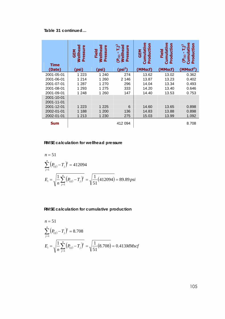
105
Table 31 continued…
Time
GEM
W
ellh
ead
Pre
ssu
re
Fiel
d W
ellh
ead
Pre
ssu
re
(P(i
j) -
Tj)
2
Wel
lhea
d P
ress
ure
GEM
C
um
ula
tive
P
rodu
ctio
n
Fiel
d C
um
ula
tive
P
rodu
ctio
n
(P(i
j) -
Tj)
2
Cu
mu
lati
ve
Pro
duct
ion
(Date) (psi) (psi) (psi2) (MMscf) (MMscf) (MMscf2) 2001-05-01 1 223 1 240 274 13.62 13.02 0.362 2001-06-01 1 214 1 260 2 146 13.87 13.23 0.402 2001-07-01 1 287 1 270 296 14.04 13.34 0.493 2001-08-01 1 293 1 275 333 14.20 13.40 0.646 2001-09-01 1 248 1 260 147 14.40 13.53 0.753 2001-10-01 2001-11-01 2001-12-01 1 223 1 225 6 14.60 13.65 0.898 2002-01-01 1 188 1 200 136 14.83 13.88 0.898 2002-01-01 1 213 1 230 275 15.03 13.99 1.092
Sum 412 094 8.708
RMSE calculation for wellhead pressure
( )( )
( )( ) ( ) psiTPn
E
TP
n
n
jjiji
n
jjij
89.894120945111
412094
51
1
2
1
2
==−=
=−
=
∑
∑
=
=
RMSE calculation for cumulative production
( )( )
( )( ) ( ) MMscfTPn
E
TP
n
n
jjiji
n
jjij
413.0708.85111
708.8
51
1
2
1
2
==−=
=−
=
∑
∑
=
=
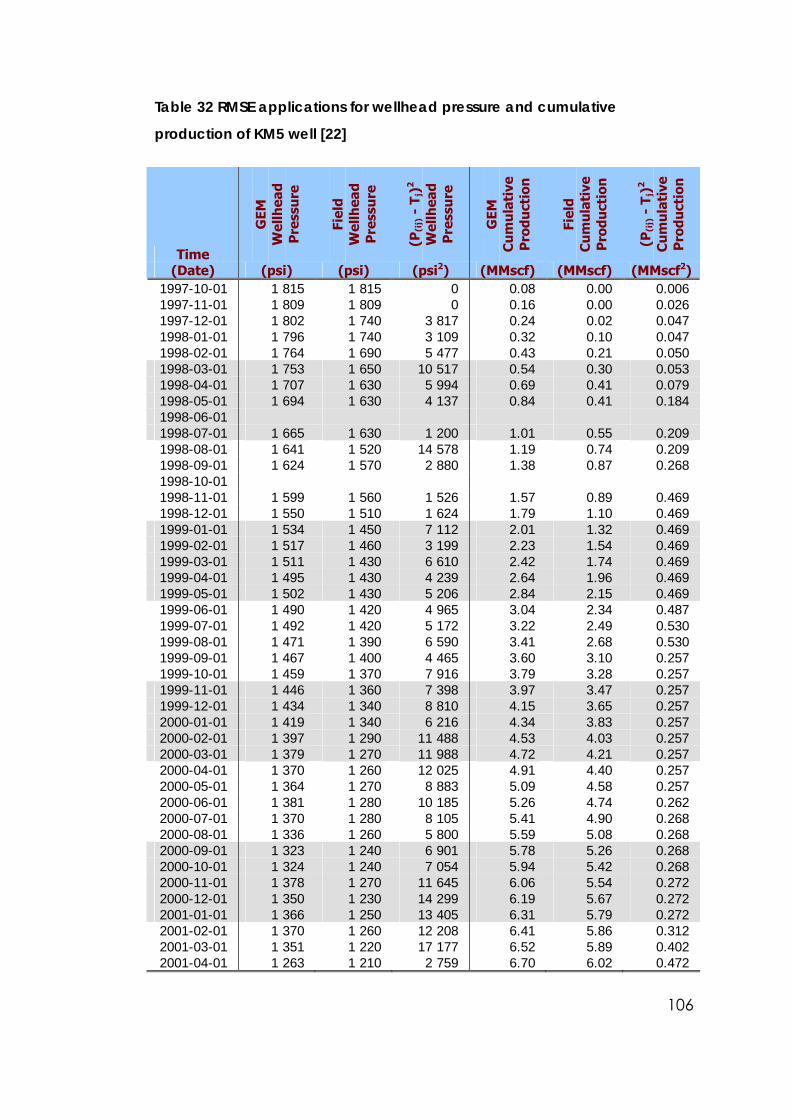
106
Table 32 RMSE applications for wellhead pressure and cumulative
production of KM5 well [22]
Time G
EM
Wel
lhea
d P
ress
ure
Fiel
d W
ellh
ead
Pre
ssu
re
(P(i
j) -
Tj)
2
Wel
lhea
d P
ress
ure
GEM
C
um
ula
tive
P
rodu
ctio
n
Fiel
d C
um
ula
tive
P
rodu
ctio
n
(P(i
j) -
Tj)
2
Cu
mu
lati
ve
Pro
duct
ion
(Date) (psi) (psi) (psi2) (MMscf) (MMscf) (MMscf2) 1997-10-01 1 815 1 815 0 0.08 0.00 0.006 1997-11-01 1 809 1 809 0 0.16 0.00 0.026 1997-12-01 1 802 1 740 3 817 0.24 0.02 0.047 1998-01-01 1 796 1 740 3 109 0.32 0.10 0.047 1998-02-01 1 764 1 690 5 477 0.43 0.21 0.050 1998-03-01 1 753 1 650 10 517 0.54 0.30 0.053 1998-04-01 1 707 1 630 5 994 0.69 0.41 0.079 1998-05-01 1 694 1 630 4 137 0.84 0.41 0.184 1998-06-01 1998-07-01 1 665 1 630 1 200 1.01 0.55 0.209 1998-08-01 1 641 1 520 14 578 1.19 0.74 0.209 1998-09-01 1 624 1 570 2 880 1.38 0.87 0.268 1998-10-01 1998-11-01 1 599 1 560 1 526 1.57 0.89 0.469 1998-12-01 1 550 1 510 1 624 1.79 1.10 0.469 1999-01-01 1 534 1 450 7 112 2.01 1.32 0.469 1999-02-01 1 517 1 460 3 199 2.23 1.54 0.469 1999-03-01 1 511 1 430 6 610 2.42 1.74 0.469 1999-04-01 1 495 1 430 4 239 2.64 1.96 0.469 1999-05-01 1 502 1 430 5 206 2.84 2.15 0.469 1999-06-01 1 490 1 420 4 965 3.04 2.34 0.487 1999-07-01 1 492 1 420 5 172 3.22 2.49 0.530 1999-08-01 1 471 1 390 6 590 3.41 2.68 0.530 1999-09-01 1 467 1 400 4 465 3.60 3.10 0.257 1999-10-01 1 459 1 370 7 916 3.79 3.28 0.257 1999-11-01 1 446 1 360 7 398 3.97 3.47 0.257 1999-12-01 1 434 1 340 8 810 4.15 3.65 0.257 2000-01-01 1 419 1 340 6 216 4.34 3.83 0.257 2000-02-01 1 397 1 290 11 488 4.53 4.03 0.257 2000-03-01 1 379 1 270 11 988 4.72 4.21 0.257 2000-04-01 1 370 1 260 12 025 4.91 4.40 0.257 2000-05-01 1 364 1 270 8 883 5.09 4.58 0.257 2000-06-01 1 381 1 280 10 185 5.26 4.74 0.262 2000-07-01 1 370 1 280 8 105 5.41 4.90 0.268 2000-08-01 1 336 1 260 5 800 5.59 5.08 0.268 2000-09-01 1 323 1 240 6 901 5.78 5.26 0.268 2000-10-01 1 324 1 240 7 054 5.94 5.42 0.268 2000-11-01 1 378 1 270 11 645 6.06 5.54 0.272 2000-12-01 1 350 1 230 14 299 6.19 5.67 0.272 2001-01-01 1 366 1 250 13 405 6.31 5.79 0.272 2001-02-01 1 370 1 260 12 208 6.41 5.86 0.312 2001-03-01 1 351 1 220 17 177 6.52 5.89 0.402 2001-04-01 1 263 1 210 2 759 6.70 6.02 0.472
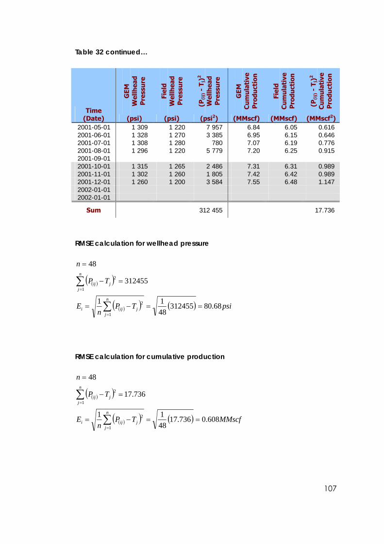
107
Table 32 continued…
Time
GEM
W
ellh
ead
Pre
ssu
re
Fiel
d W
ellh
ead
Pre
ssu
re
(P(i
j) -
Tj)
2
Wel
lhea
d P
ress
ure
GEM
C
um
ula
tive
P
rodu
ctio
n
Fiel
d C
um
ula
tive
P
rodu
ctio
n
(P(i
j) -
Tj)
2
Cu
mu
lati
ve
Pro
duct
ion
(Date) (psi) (psi) (psi2) (MMscf) (MMscf) (MMscf2) 2001-05-01 1 309 1 220 7 957 6.84 6.05 0.616 2001-06-01 1 328 1 270 3 385 6.95 6.15 0.646 2001-07-01 1 308 1 280 780 7.07 6.19 0.776 2001-08-01 1 296 1 220 5 779 7.20 6.25 0.915 2001-09-01 2001-10-01 1 315 1 265 2 486 7.31 6.31 0.989 2001-11-01 1 302 1 260 1 805 7.42 6.42 0.989 2001-12-01 1 260 1 200 3 584 7.55 6.48 1.147 2002-01-01 2002-01-01
Sum 312 455 17.736
RMSE calculation for wellhead pressure
( )( )
( )( ) ( ) psiTPn
E
TP
n
n
jjiji
n
jjij
68.803124554811
312455
48
1
2
1
2
==−=
=−
=
∑
∑
=
=
RMSE calculation for cumulative production
( )( )
( )( ) ( ) MMscfTPn
E
TP
n
n
jjiji
n
jjij
608.0736.174811
736.17
48
1
2
1
2
==−=
=−
=
∑
∑
=
=
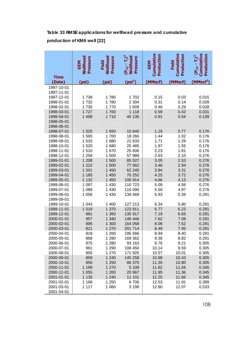
108
Table 33 RMSE applications for wellhead pressure and cumulative
production of KM6 well [22]
Time G
EM
Wel
lhea
d P
ress
ure
Fiel
d W
ellh
ead
Pre
ssu
re
(P(i
j) -
Tj)
2
Wel
lhea
d P
ress
ure
GEM
C
um
ula
tive
P
rodu
ctio
n
Fiel
d C
um
ula
tive
P
rodu
ctio
n
(P(i
j) -
Tj)
2
Cu
mu
lati
ve
Pro
duct
ion
(Date) (psi) (psi) (psi2) (MMscf) (MMscf) (MMscf2) 1997-10-01 1997-11-01 1997-12-01 1 739 1 780 1 702 0.15 0.03 0.015 1998-01-01 1 732 1 780 2 304 0.31 0.14 0.028 1998-02-01 1 730 1 770 1 609 0.46 0.29 0.028 1998-03-01 1 727 1 760 1 118 0.59 0.42 0.031 1998-04-01 1 498 1 710 45 135 0.91 0.54 0.139 1998-05-01 1998-06-01 1998-07-01 1 525 1 650 15 640 1.19 0.77 0.176 1998-08-01 1 565 1 700 18 266 1.44 1.02 0.176 1998-09-01 1 533 1 680 21 633 1.71 1.29 0.176 1998-10-01 1 520 1 680 25 485 1.97 1.55 0.176 1998-11-01 1 510 1 670 25 606 2.23 1.81 0.176 1998-12-01 1 259 1 500 57 989 2.63 2.10 0.276 1999-01-01 1 208 1 500 85 527 3.05 2.53 0.276 1999-02-01 1 222 1 500 77 562 3.46 2.94 0.276 1999-03-01 1 201 1 450 62 245 3.84 3.31 0.276 1999-04-01 1 185 1 450 70 252 4.25 3.72 0.276 1999-05-01 1 132 1 450 100 914 4.66 4.13 0.276 1999-06-01 1 097 1 430 110 723 5.09 4.56 0.276 1999-07-01 1 089 1 430 116 090 5.50 4.97 0.276 1999-08-01 1 056 1 430 139 569 5.93 5.39 0.291 1999-09-01 1999-10-01 1 043 1 400 127 213 6.34 5.80 0.291 1999-11-01 1 018 1 370 123 911 6.77 6.23 0.291 1999-12-01 981 1 350 135 917 7.19 6.65 0.291 2000-01-01 957 1 340 146 446 7.62 7.08 0.291 2000-02-01 895 1 300 164 058 8.06 7.52 0.291 2000-03-01 821 1 270 201 714 8.49 7.95 0.291 2000-04-01 818 1 260 195 566 8.94 8.40 0.291 2000-05-01 868 1 280 169 362 9.36 8.82 0.291 2000-06-01 975 1 280 93 163 9.76 9.21 0.305 2000-07-01 961 1 290 108 450 10.14 9.59 0.305 2000-08-01 855 1 270 171 925 10.57 10.01 0.305 2000-09-01 859 1 240 145 258 10.98 10.43 0.305 2000-10-01 956 1 250 86 375 11.35 10.80 0.305 2000-11-01 1 199 1 270 5 109 11.62 11.04 0.345 2000-12-01 1 055 1 200 20 967 11.95 11.36 0.345 2001-01-01 1 135 1 240 11 101 12.25 11.66 0.345 2001-02-01 1 168 1 250 6 706 12.53 11.91 0.389 2001-03-01 1 117 1 060 3 199 12.80 12.07 0.533 2001-04-01
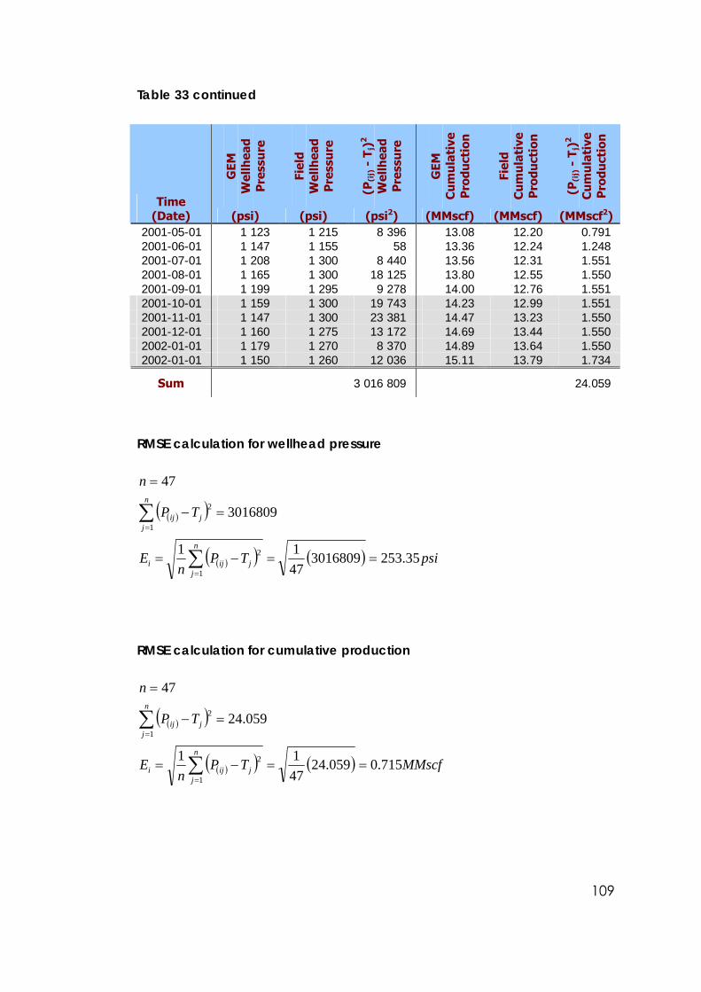
109
Table 33 continued
Time
GEM
W
ellh
ead
Pre
ssu
re
Fiel
d W
ellh
ead
Pre
ssu
re
(P(i
j) -
Tj)
2
Wel
lhea
d P
ress
ure
GEM
C
um
ula
tive
P
rodu
ctio
n
Fiel
d C
um
ula
tive
P
rodu
ctio
n
(P(i
j) -
Tj)
2
Cu
mu
lati
ve
Pro
duct
ion
(Date) (psi) (psi) (psi2) (MMscf) (MMscf) (MMscf2) 2001-05-01 1 123 1 215 8 396 13.08 12.20 0.791 2001-06-01 1 147 1 155 58 13.36 12.24 1.248 2001-07-01 1 208 1 300 8 440 13.56 12.31 1.551 2001-08-01 1 165 1 300 18 125 13.80 12.55 1.550 2001-09-01 1 199 1 295 9 278 14.00 12.76 1.551 2001-10-01 1 159 1 300 19 743 14.23 12.99 1.551 2001-11-01 1 147 1 300 23 381 14.47 13.23 1.550 2001-12-01 1 160 1 275 13 172 14.69 13.44 1.550 2002-01-01 1 179 1 270 8 370 14.89 13.64 1.550 2002-01-01 1 150 1 260 12 036 15.11 13.79 1.734
Sum 3 016 809 24.059
RMSE calculation for wellhead pressure
( )( )
( )( ) ( ) psiTPn
E
TP
n
n
jjiji
n
jjij
35.25330168094711
3016809
47
1
2
1
2
==−=
=−
=
∑
∑
=
=
RMSE calculation for cumulative production
( )( )
( )( ) ( ) MMscfTPn
E
TP
n
n
jjiji
n
jjij
715.0059.244711
059.24
47
1
2
1
2
==−=
=−
=
∑
∑
=
=
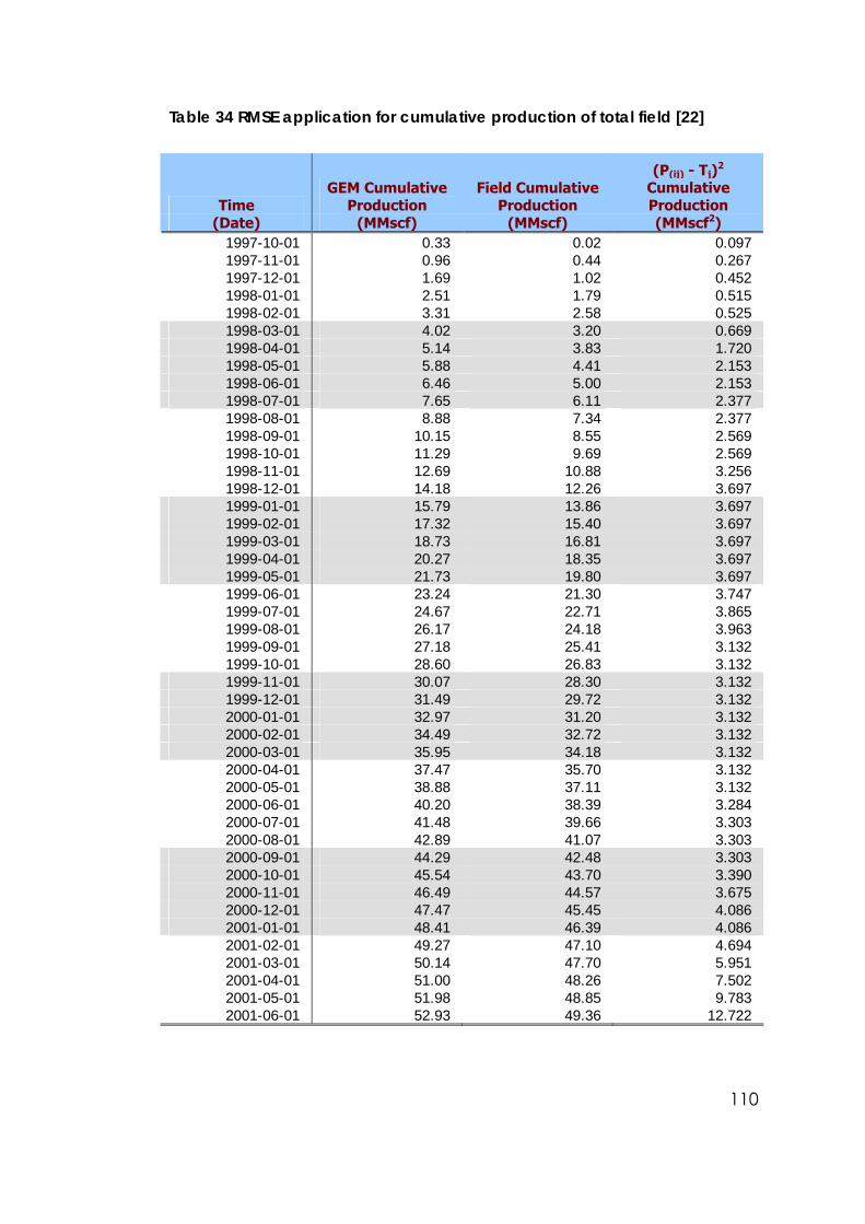
110
Table 34 RMSE application for cumulative production of total field [22]
Time GEM Cumulative
Production Field Cumulative
Production
(P(ij) - Tj)2
Cumulative Production
(Date) (MMscf) (MMscf) (MMscf2) 1997-10-01 0.33 0.02 0.097 1997-11-01 0.96 0.44 0.267 1997-12-01 1.69 1.02 0.452 1998-01-01 2.51 1.79 0.515 1998-02-01 3.31 2.58 0.525 1998-03-01 4.02 3.20 0.669 1998-04-01 5.14 3.83 1.720 1998-05-01 5.88 4.41 2.153 1998-06-01 6.46 5.00 2.153 1998-07-01 7.65 6.11 2.377 1998-08-01 8.88 7.34 2.377 1998-09-01 10.15 8.55 2.569 1998-10-01 11.29 9.69 2.569 1998-11-01 12.69 10.88 3.256 1998-12-01 14.18 12.26 3.697 1999-01-01 15.79 13.86 3.697 1999-02-01 17.32 15.40 3.697 1999-03-01 18.73 16.81 3.697 1999-04-01 20.27 18.35 3.697 1999-05-01 21.73 19.80 3.697 1999-06-01 23.24 21.30 3.747 1999-07-01 24.67 22.71 3.865 1999-08-01 26.17 24.18 3.963 1999-09-01 27.18 25.41 3.132 1999-10-01 28.60 26.83 3.132 1999-11-01 30.07 28.30 3.132 1999-12-01 31.49 29.72 3.132 2000-01-01 32.97 31.20 3.132 2000-02-01 34.49 32.72 3.132 2000-03-01 35.95 34.18 3.132 2000-04-01 37.47 35.70 3.132 2000-05-01 38.88 37.11 3.132 2000-06-01 40.20 38.39 3.284 2000-07-01 41.48 39.66 3.303 2000-08-01 42.89 41.07 3.303 2000-09-01 44.29 42.48 3.303 2000-10-01 45.54 43.70 3.390 2000-11-01 46.49 44.57 3.675 2000-12-01 47.47 45.45 4.086 2001-01-01 48.41 46.39 4.086 2001-02-01 49.27 47.10 4.694 2001-03-01 50.14 47.70 5.951 2001-04-01 51.00 48.26 7.502 2001-05-01 51.98 48.85 9.783 2001-06-01 52.93 49.36 12.722
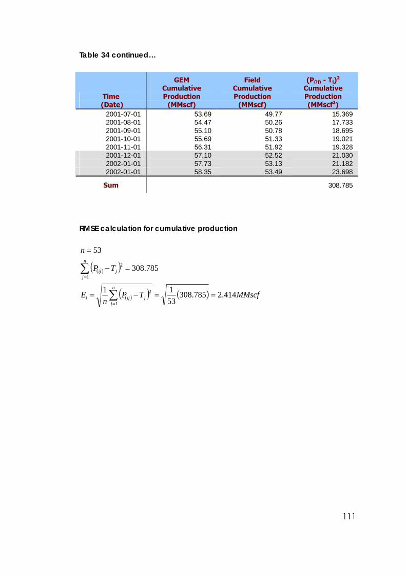
111
Table 34 continued…
Time
GEM Cumulative Production
Field Cumulative Production
(P(ij) - Tj)2
Cumulative Production
(Date) (MMscf) (MMscf) (MMscf2) 2001-07-01 53.69 49.77 15.369 2001-08-01 54.47 50.26 17.733 2001-09-01 55.10 50.78 18.695 2001-10-01 55.69 51.33 19.021 2001-11-01 56.31 51.92 19.328 2001-12-01 57.10 52.52 21.030 2002-01-01 57.73 53.13 21.182 2002-01-01 58.35 53.49 23.698
Sum 308.785
RMSE calculation for cumulative production
( )( )
( )( ) ( ) MMscfTPn
E
TP
n
n
jjiji
n
jjij
414.2785.3085311
785.308
53
1
2
1
2
==−=
=−
=
∑
∑
=
=
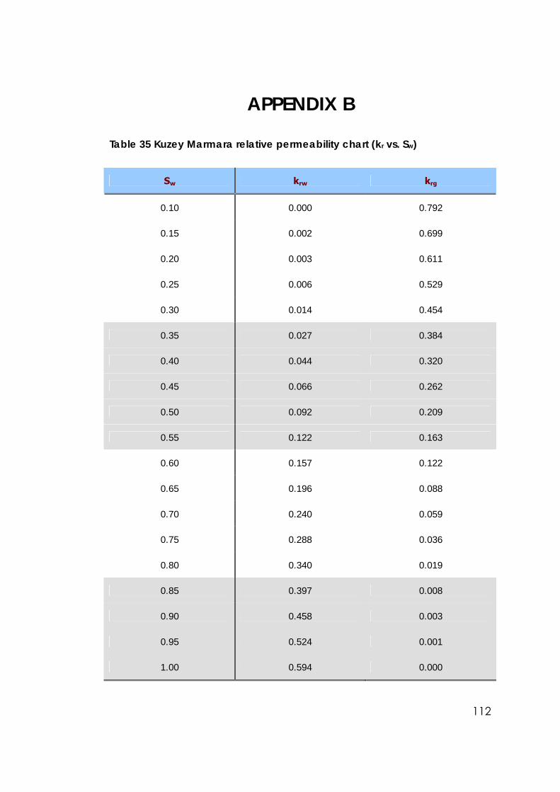
112
APPENDIX B
Table 35 Kuzey Marmara relative permeability chart (kr vs. Sw)
Sw krw krg
0.10 0.000 0.792
0.15 0.002 0.699
0.20 0.003 0.611
0.25 0.006 0.529
0.30 0.014 0.454
0.35 0.027 0.384
0.40 0.044 0.320
0.45 0.066 0.262
0.50 0.092 0.209
0.55 0.122 0.163
0.60 0.157 0.122
0.65 0.196 0.088
0.70 0.240 0.059
0.75 0.288 0.036
0.80 0.340 0.019
0.85 0.397 0.008
0.90 0.458 0.003
0.95 0.524 0.001
1.00 0.594 0.000
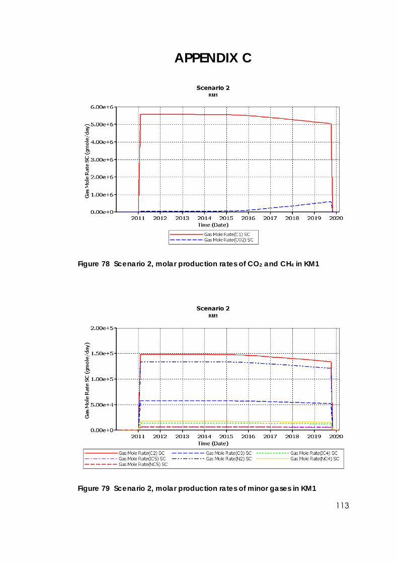
113
APPENDIX C
Figure 78 Scenario 2, molar production rates of CO2 and CH4 in KM1
Figure 79 Scenario 2, molar production rates of minor gases in KM1
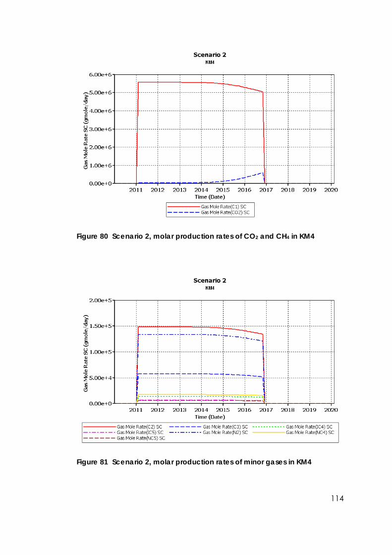
114
Figure 80 Scenario 2, molar production rates of CO2 and CH4 in KM4
Figure 81 Scenario 2, molar production rates of minor gases in KM4
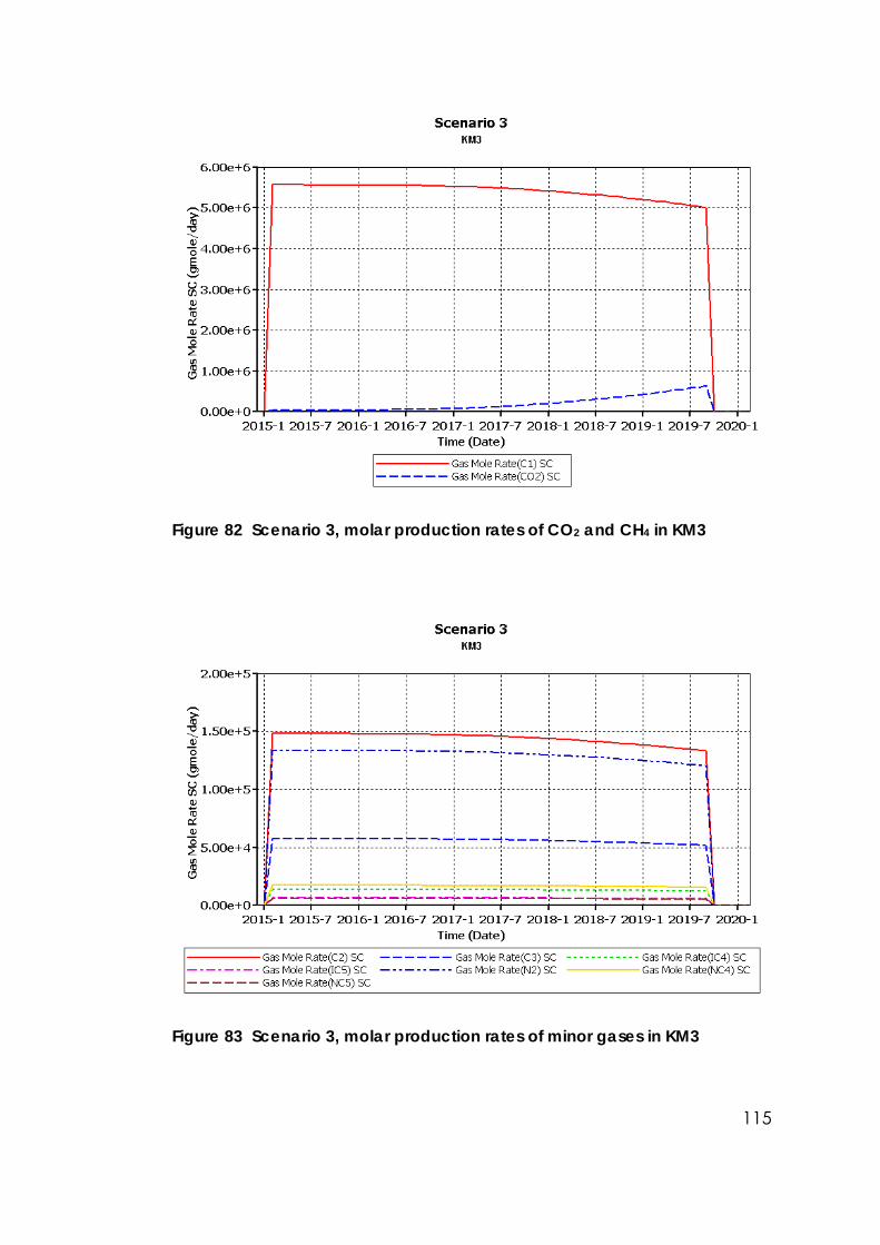
115
Figure 82 Scenario 3, molar production rates of CO2 and CH4 in KM3
Figure 83 Scenario 3, molar production rates of minor gases in KM3
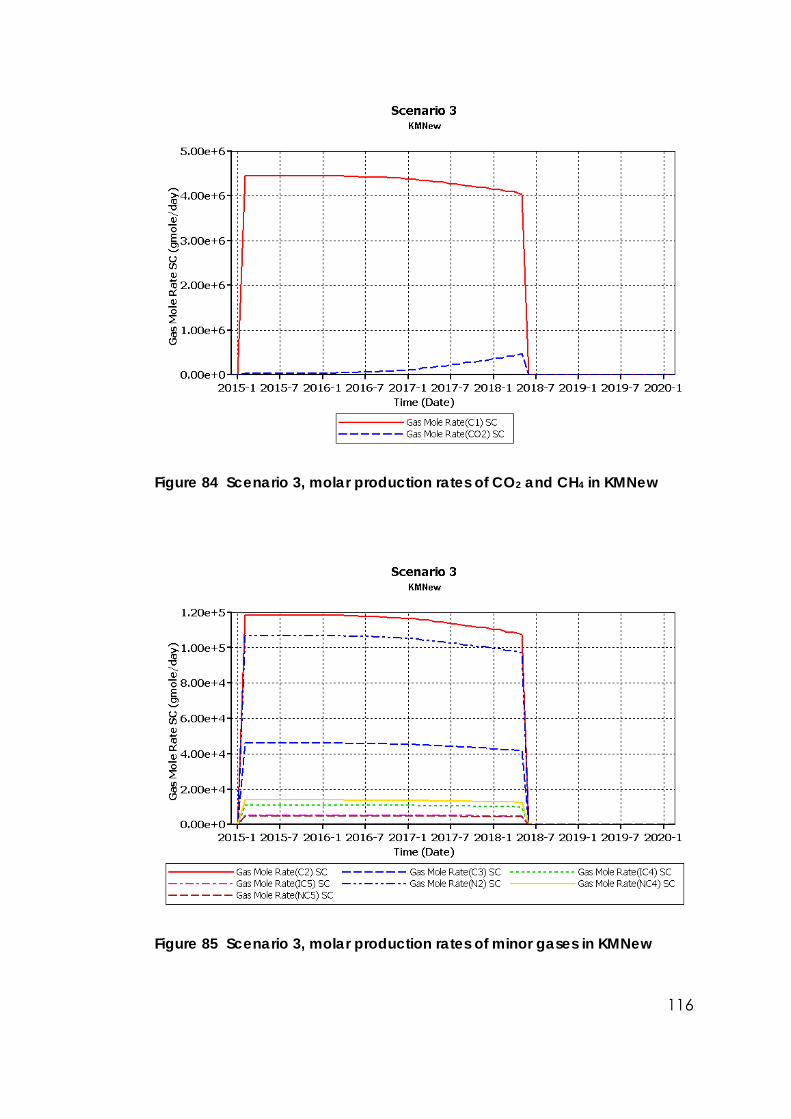
116
Figure 84 Scenario 3, molar production rates of CO2 and CH4 in KMNew
Figure 85 Scenario 3, molar production rates of minor gases in KMNew
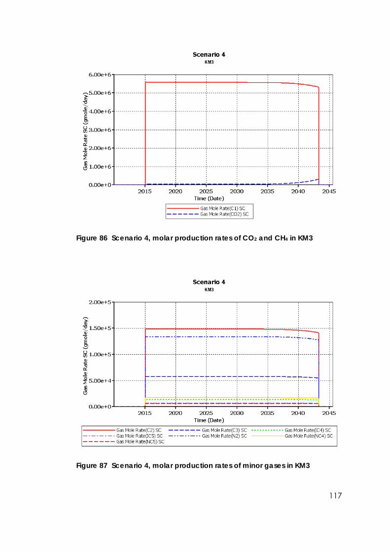
117
Figure 86 Scenario 4, molar production rates of CO2 and CH4 in KM3
Figure 87 Scenario 4, molar production rates of minor gases in KM3
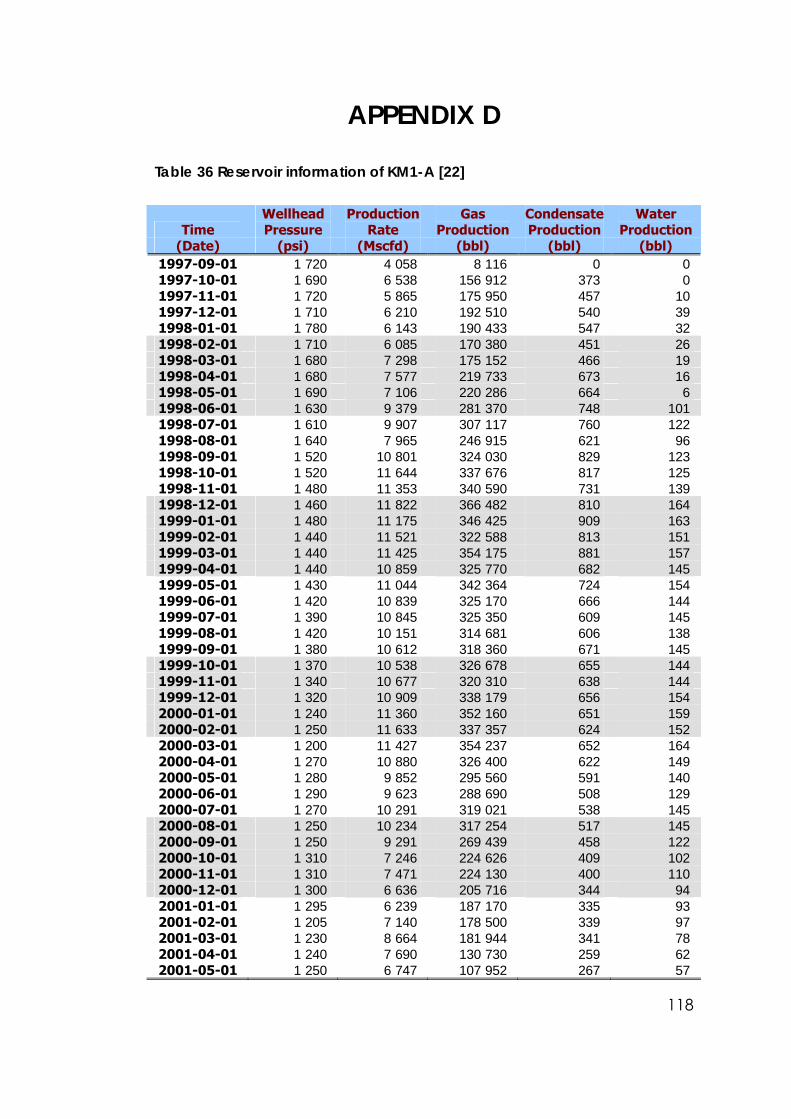
118
APPENDIX D
Table 36 Reservoir information of KM1-A [22]
Time Wellhead Pressure
Production Rate
Gas Production
Condensate Production
Water Production
(Date) (psi) (Mscfd) (bbl) (bbl) (bbl) 1997-09-01 1 720 4 058 8 116 0 0 1997-10-01 1 690 6 538 156 912 373 0 1997-11-01 1 720 5 865 175 950 457 10 1997-12-01 1 710 6 210 192 510 540 39 1998-01-01 1 780 6 143 190 433 547 32 1998-02-01 1 710 6 085 170 380 451 26 1998-03-01 1 680 7 298 175 152 466 19 1998-04-01 1 680 7 577 219 733 673 16 1998-05-01 1 690 7 106 220 286 664 6 1998-06-01 1 630 9 379 281 370 748 101 1998-07-01 1 610 9 907 307 117 760 122 1998-08-01 1 640 7 965 246 915 621 96 1998-09-01 1 520 10 801 324 030 829 123 1998-10-01 1 520 11 644 337 676 817 125 1998-11-01 1 480 11 353 340 590 731 139 1998-12-01 1 460 11 822 366 482 810 164 1999-01-01 1 480 11 175 346 425 909 163 1999-02-01 1 440 11 521 322 588 813 151 1999-03-01 1 440 11 425 354 175 881 157 1999-04-01 1 440 10 859 325 770 682 145 1999-05-01 1 430 11 044 342 364 724 154 1999-06-01 1 420 10 839 325 170 666 144 1999-07-01 1 390 10 845 325 350 609 145 1999-08-01 1 420 10 151 314 681 606 138 1999-09-01 1 380 10 612 318 360 671 145 1999-10-01 1 370 10 538 326 678 655 144 1999-11-01 1 340 10 677 320 310 638 144 1999-12-01 1 320 10 909 338 179 656 154 2000-01-01 1 240 11 360 352 160 651 159 2000-02-01 1 250 11 633 337 357 624 152 2000-03-01 1 200 11 427 354 237 652 164 2000-04-01 1 270 10 880 326 400 622 149 2000-05-01 1 280 9 852 295 560 591 140 2000-06-01 1 290 9 623 288 690 508 129 2000-07-01 1 270 10 291 319 021 538 145 2000-08-01 1 250 10 234 317 254 517 145 2000-09-01 1 250 9 291 269 439 458 122 2000-10-01 1 310 7 246 224 626 409 102 2000-11-01 1 310 7 471 224 130 400 110 2000-12-01 1 300 6 636 205 716 344 94 2001-01-01 1 295 6 239 187 170 335 93 2001-02-01 1 205 7 140 178 500 339 97 2001-03-01 1 230 8 664 181 944 341 78 2001-04-01 1 240 7 690 130 730 259 62 2001-05-01 1 250 6 747 107 952 267 57
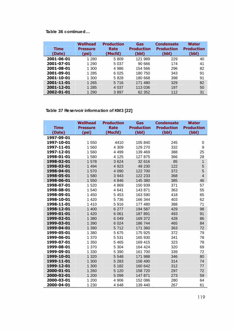
119
Table 36 continued…
Time Wellhead Pressure
Production Rate
Gas Production
Condensate Production
Water Production
(Date) (psi) (Mscfd) (bbl) (bbl) (bbl) 2001-06-01 1 280 5 809 121 989 229 40 2001-07-01 1 290 5 037 90 666 174 41 2001-08-01 1 300 4 986 154 566 296 82 2001-09-01 1 285 6 025 180 750 343 91 2001-10-01 1 300 5 828 180 668 398 91 2001-11-01 1 265 5 716 171 480 329 82 2001-12-01 1 285 4 037 113 036 197 50 2002-01-01 1 290 3 897 62 352 112 31
Table 37 Reservoir information of KM3 [22]
Time Wellhead Pressure
Production Rate
Gas Production
Condensate Production
Water Production
(Date) (psi) (Mscfd) (bbl) (bbl) (bbl) 1997-09-01 1997-10-01 1 550 4410 105 840 245 0 1997-11-01 1 560 4 309 129 270 332 9 1997-12-01 1 560 4 499 139 469 388 25 1998-01-01 1 580 4 125 127 875 366 28 1998-02-01 1 578 3 624 32 616 85 1 1998-03-01 1 494 4 923 49 230 122 5 1998-04-01 1 570 4 090 122 700 372 5 1998-05-01 1 580 3 943 122 233 368 4 1998-06-01 1 550 4 846 145 380 385 46 1998-07-01 1 520 4 869 150 939 371 57 1998-08-01 1 540 4 641 143 871 363 55 1998-09-01 1 450 5 453 163 590 418 65 1998-10-01 1 420 5 736 166 344 403 62 1998-11-01 1 410 5 916 177 480 388 71 1998-12-01 1 400 6 277 194 587 429 98 1999-01-01 1 420 6 061 187 891 493 91 1999-02-01 1 380 6 049 169 372 428 86 1999-03-01 1 390 6 024 186 744 465 84 1999-04-01 1 390 5 712 171 360 363 72 1999-05-01 1 380 5 675 175 925 372 79 1999-06-01 1 370 5 531 165 930 341 78 1999-07-01 1 350 5 465 169 415 323 78 1999-08-01 1 370 5 304 164 424 320 69 1999-09-01 1 330 5 390 161 700 339 72 1999-10-01 1 320 5 548 171 988 346 80 1999-11-01 1 300 5 283 158 490 314 74 1999-12-01 1 300 5 182 160 642 312 77 2000-01-01 1 260 5 120 158 720 297 72 2000-02-01 1 200 5 099 147 871 273 59 2000-03-01 1 200 4 906 152 086 280 64 2000-04-01 1 230 4 648 139 440 267 61
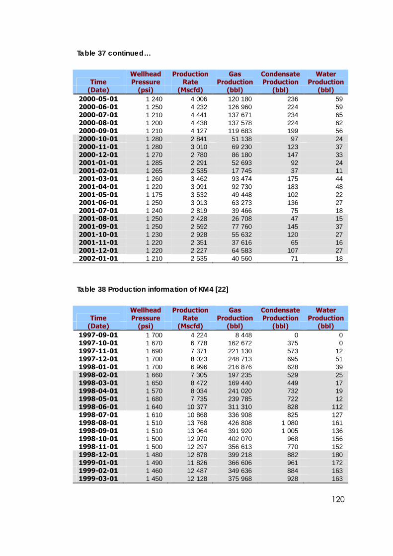
120
Table 37 continued…
Time Wellhead Pressure
Production Rate
Gas Production
Condensate Production
Water Production
(Date) (psi) (Mscfd) (bbl) (bbl) (bbl) 2000-05-01 1 240 4 006 120 180 236 59 2000-06-01 1 250 4 232 126 960 224 59 2000-07-01 1 210 4 441 137 671 234 65 2000-08-01 1 200 4 438 137 578 224 62 2000-09-01 1 210 4 127 119 683 199 56 2000-10-01 1 280 2 841 51 138 97 24 2000-11-01 1 280 3 010 69 230 123 37 2000-12-01 1 270 2 780 86 180 147 33 2001-01-01 1 285 2 291 52 693 92 24 2001-02-01 1 265 2 535 17 745 37 11 2001-03-01 1 260 3 462 93 474 175 44 2001-04-01 1 220 3 091 92 730 183 48 2001-05-01 1 175 3 532 49 448 102 22 2001-06-01 1 250 3 013 63 273 136 27 2001-07-01 1 240 2 819 39 466 75 18 2001-08-01 1 250 2 428 26 708 47 15 2001-09-01 1 250 2 592 77 760 145 37 2001-10-01 1 230 2 928 55 632 120 27 2001-11-01 1 220 2 351 37 616 65 16 2001-12-01 1 220 2 227 64 583 107 27 2002-01-01 1 210 2 535 40 560 71 18
Table 38 Production information of KM4 [22]
Time Wellhead Pressure
Production Rate
Gas Production
Condensate Production
Water Production
(Date) (psi) (Mscfd) (bbl) (bbl) (bbl) 1997-09-01 1 700 4 224 8 448 0 0 1997-10-01 1 670 6 778 162 672 375 0 1997-11-01 1 690 7 371 221 130 573 12 1997-12-01 1 700 8 023 248 713 695 51 1998-01-01 1 700 6 996 216 876 628 39 1998-02-01 1 660 7 305 197 235 529 25 1998-03-01 1 650 8 472 169 440 449 17 1998-04-01 1 570 8 034 241 020 732 19 1998-05-01 1 680 7 735 239 785 722 12 1998-06-01 1 640 10 377 311 310 828 112 1998-07-01 1 610 10 868 336 908 825 127 1998-08-01 1 510 13 768 426 808 1 080 161 1998-09-01 1 510 13 064 391 920 1 005 136 1998-10-01 1 500 12 970 402 070 968 156 1998-11-01 1 500 12 297 356 613 770 152 1998-12-01 1 480 12 878 399 218 882 180 1999-01-01 1 490 11 826 366 606 961 172 1999-02-01 1 460 12 487 349 636 884 163 1999-03-01 1 450 12 128 375 968 928 163
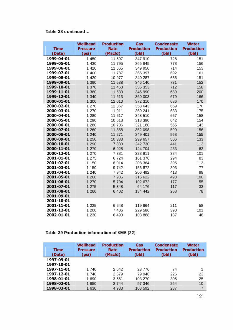
121
Table 38 continued…
Time Wellhead Pressure
Production Rate
Gas Production
Condensate Production
Water Production
(Date) (psi) (Mscfd) (bbl) (bbl) (bbl) 1999-04-01 1 450 11 597 347 910 728 151 1999-05-01 1 430 11 795 365 645 778 156 1999-06-01 1 420 11 665 349 950 714 153 1999-07-01 1 400 11 787 365 397 692 161 1999-08-01 1 420 10 977 340 287 655 151 1999-09-01 1 390 11 538 346 140 731 152 1999-10-01 1 370 11 463 355 353 712 158 1999-11-01 1 360 11 533 345 990 689 200 1999-12-01 1 340 11 613 360 003 679 166 2000-01-01 1 300 12 010 372 310 686 170 2000-02-01 1 270 12 367 358 643 669 170 2000-03-01 1 270 11 911 369 241 683 175 2000-04-01 1 280 11 617 348 510 667 158 2000-05-01 1 290 10 613 318 390 642 154 2000-06-01 1 280 10 706 321 180 565 143 2000-07-01 1 260 11 358 352 098 590 156 2000-08-01 1 240 11 271 349 401 568 155 2000-09-01 1 250 10 333 299 657 506 133 2000-10-01 1 290 7 830 242 730 441 113 2000-11-01 1 270 6 928 124 704 233 62 2000-12-01 1 270 7 381 228 811 384 101 2001-01-01 1 275 6 724 161 376 294 83 2001-02-01 1 150 8 014 208 364 395 113 2001-03-01 1 150 9 742 155 872 303 77 2001-04-01 1 240 7 942 206 492 413 98 2001-05-01 1 260 7 986 215 622 493 100 2001-06-01 1 270 5 704 102 672 177 55 2001-07-01 1 275 5 348 64 176 117 33 2001-08-01 1 260 6 402 134 442 268 78 2001-09-01 2001-10-01 2001-11-01 1 225 6 648 119 664 211 58 2001-12-01 1 200 7 406 229 586 390 101 2002-01-01 1 230 6 493 103 888 187 48
Table 39 Production information of KM5 [22]
Time Wellhead Pressure
Production Rate
Gas Production
Condensate Production
Water Production
(Date) (psi) (Mscfd) (bbl) (bbl) (bbl) 1997-09-01 1997-10-01 1997-11-01 1 740 2 642 23 776 74 1 1997-12-01 1 740 2 579 79 946 226 23 1998-01-01 1 690 3 561 103 270 305 25 1998-02-01 1 650 3 744 97 346 264 10 1998-03-01 1 630 4 933 103 592 287 7
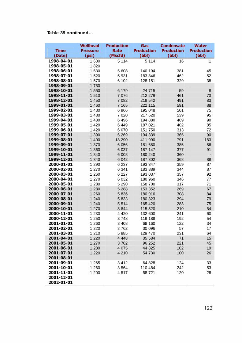
122
Table 39 continued…
Time Wellhead Pressure
Production Rate
Gas Production
Condensate Production
Water Production
(Date) (psi) (Mscfd) (bbl) (bbl) (bbl) 1998-04-01 1 630 5 114 5 114 16 1 1998-05-01 1 820 1998-06-01 1 630 5 608 140 194 381 45 1998-07-01 1 520 5 931 183 846 462 52 1998-08-01 1 570 6 102 128 151 329 38 1998-09-01 1 780 1998-10-01 1 560 6 179 24 715 59 8 1998-11-01 1 510 7 076 212 279 461 73 1998-12-01 1 450 7 082 219 542 491 83 1999-01-01 1 460 7 165 222 115 591 88 1999-02-01 1 430 6 966 195 048 501 75 1999-03-01 1 430 7 020 217 620 539 95 1999-04-01 1 430 6 496 194 880 409 90 1999-05-01 1 420 6 449 187 021 402 85 1999-06-01 1 420 6 070 151 750 313 72 1999-07-01 1 390 6 269 194 339 365 90 1999-08-01 1 400 13 290 411 990 791 183 1999-09-01 1 370 6 056 181 680 385 86 1999-10-01 1 360 6 037 187 147 377 91 1999-11-01 1 340 6 008 180 240 360 - 1999-12-01 1 340 6 042 187 302 368 88 2000-01-01 1 290 6 237 193 347 359 87 2000-02-01 1 270 6 341 183 889 344 87 2000-03-01 1 260 6 227 193 037 357 92 2000-04-01 1 270 6 032 180 960 346 77 2000-05-01 1 280 5 290 158 700 317 71 2000-06-01 1 280 5 288 153 352 269 67 2000-07-01 1 260 5 836 180 916 308 84 2000-08-01 1 240 5 833 180 823 294 79 2000-09-01 1 240 5 514 165 420 283 75 2000-10-01 1 270 3 844 115 320 210 54 2000-11-01 1 230 4 420 132 600 241 60 2000-12-01 1 250 3 748 116 188 192 54 2001-01-01 1 260 3 408 68 160 122 34 2001-02-01 1 220 3 762 30 096 57 17 2001-03-01 1 210 5 885 129 470 231 64 2001-04-01 1 220 4 448 35 584 71 15 2001-05-01 1 270 3 702 96 252 221 45 2001-06-01 1 280 4 075 44 825 102 19 2001-07-01 1 220 4 210 54 730 100 26 2001-08-01 2001-09-01 1 265 3 412 64 828 124 33 2001-10-01 1 260 3 564 110 484 242 53 2001-11-01 1 200 4 517 58 721 120 28 2001-12-01 2002-01-01
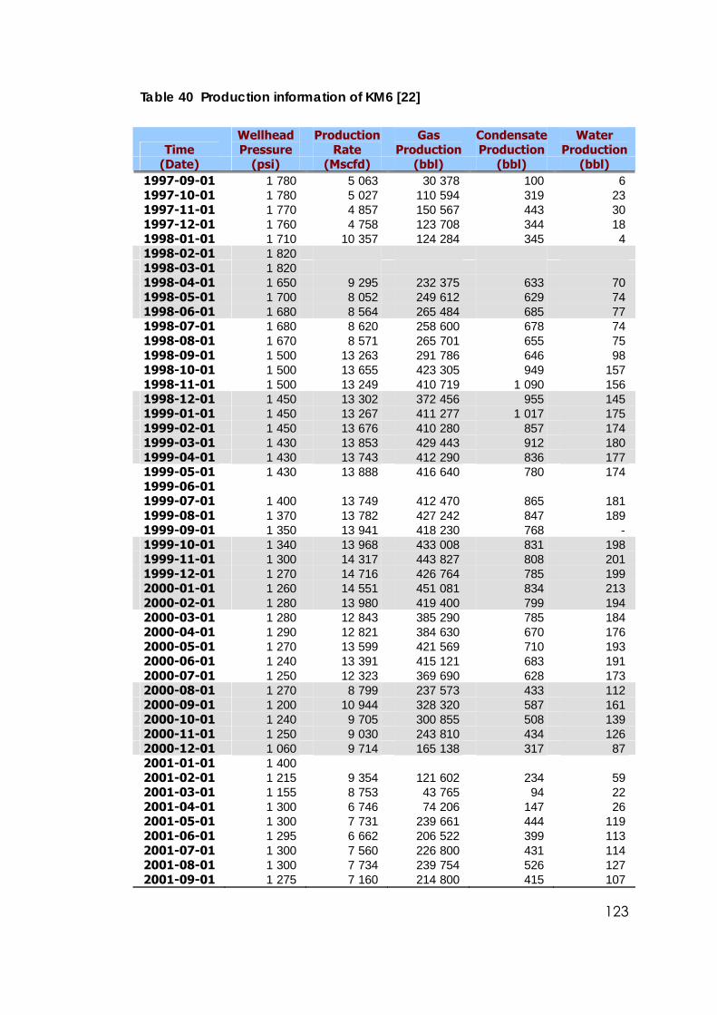
123
Table 40 Production information of KM6 [22]
Time Wellhead Pressure
Production Rate
Gas Production
Condensate Production
Water Production
(Date) (psi) (Mscfd) (bbl) (bbl) (bbl) 1997-09-01 1 780 5 063 30 378 100 6 1997-10-01 1 780 5 027 110 594 319 23 1997-11-01 1 770 4 857 150 567 443 30 1997-12-01 1 760 4 758 123 708 344 18 1998-01-01 1 710 10 357 124 284 345 4 1998-02-01 1 820 1998-03-01 1 820 1998-04-01 1 650 9 295 232 375 633 70 1998-05-01 1 700 8 052 249 612 629 74 1998-06-01 1 680 8 564 265 484 685 77 1998-07-01 1 680 8 620 258 600 678 74 1998-08-01 1 670 8 571 265 701 655 75 1998-09-01 1 500 13 263 291 786 646 98 1998-10-01 1 500 13 655 423 305 949 157 1998-11-01 1 500 13 249 410 719 1 090 156 1998-12-01 1 450 13 302 372 456 955 145 1999-01-01 1 450 13 267 411 277 1 017 175 1999-02-01 1 450 13 676 410 280 857 174 1999-03-01 1 430 13 853 429 443 912 180 1999-04-01 1 430 13 743 412 290 836 177 1999-05-01 1 430 13 888 416 640 780 174 1999-06-01 1999-07-01 1 400 13 749 412 470 865 181 1999-08-01 1 370 13 782 427 242 847 189 1999-09-01 1 350 13 941 418 230 768 - 1999-10-01 1 340 13 968 433 008 831 198 1999-11-01 1 300 14 317 443 827 808 201 1999-12-01 1 270 14 716 426 764 785 199 2000-01-01 1 260 14 551 451 081 834 213 2000-02-01 1 280 13 980 419 400 799 194 2000-03-01 1 280 12 843 385 290 785 184 2000-04-01 1 290 12 821 384 630 670 176 2000-05-01 1 270 13 599 421 569 710 193 2000-06-01 1 240 13 391 415 121 683 191 2000-07-01 1 250 12 323 369 690 628 173 2000-08-01 1 270 8 799 237 573 433 112 2000-09-01 1 200 10 944 328 320 587 161 2000-10-01 1 240 9 705 300 855 508 139 2000-11-01 1 250 9 030 243 810 434 126 2000-12-01 1 060 9 714 165 138 317 87 2001-01-01 1 400 2001-02-01 1 215 9 354 121 602 234 59 2001-03-01 1 155 8 753 43 765 94 22 2001-04-01 1 300 6 746 74 206 147 26 2001-05-01 1 300 7 731 239 661 444 119 2001-06-01 1 295 6 662 206 522 399 113 2001-07-01 1 300 7 560 226 800 431 114 2001-08-01 1 300 7 734 239 754 526 127 2001-09-01 1 275 7 160 214 800 415 107

124
Table 40 continued…
Time Wellhead Pressure
Production Rate
Gas Production
Condensate Production
Water Production
(Date) (psi) (Mscfd) (bbl) (bbl) (bbl) 2001-10-01 1 270 6 542 202 802 345 92 2001-11-01 1 260 7 171 150 591 258 56 2001-12-01 1 780 5 063 30 378 100 6 2002-01-01 1 780 5 027 110 594 319 23
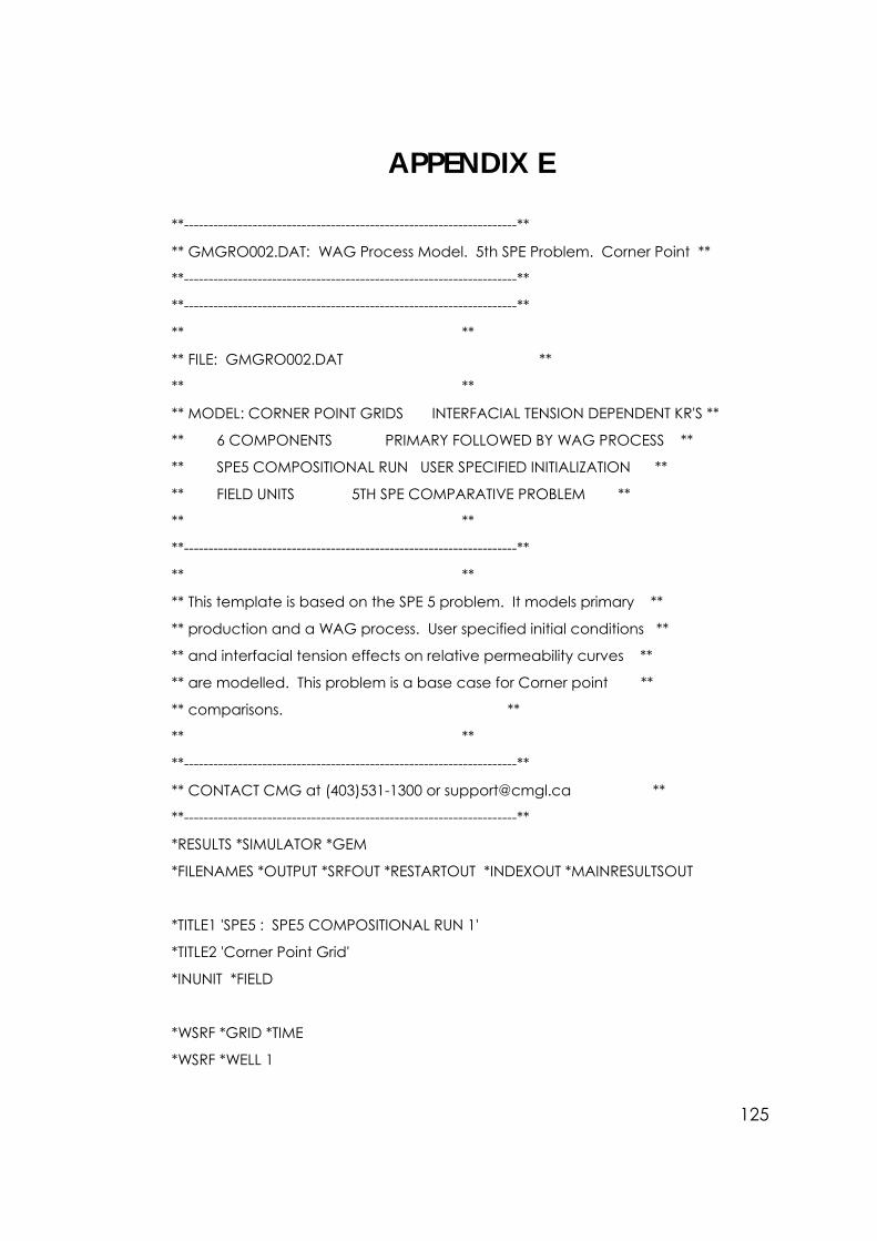
125
APPENDIX E
**--------------------------------------------------------------------**
** GMGRO002.DAT: WAG Process Model. 5th SPE Problem. Corner Point **
**--------------------------------------------------------------------**
**--------------------------------------------------------------------**
** **
** FILE: GMGRO002.DAT **
** **
** MODEL: CORNER POINT GRIDS INTERFACIAL TENSION DEPENDENT KR'S **
** 6 COMPONENTS PRIMARY FOLLOWED BY WAG PROCESS **
** SPE5 COMPOSITIONAL RUN USER SPECIFIED INITIALIZATION **
** FIELD UNITS 5TH SPE COMPARATIVE PROBLEM **
** **
**--------------------------------------------------------------------**
** **
** This template is based on the SPE 5 problem. It models primary **
** production and a WAG process. User specified initial conditions **
** and interfacial tension effects on relative permeability curves **
** are modelled. This problem is a base case for Corner point **
** comparisons. **
** **
**--------------------------------------------------------------------**
** CONTACT CMG at (403)531-1300 or [email protected] **
**--------------------------------------------------------------------**
*RESULTS *SIMULATOR *GEM
*FILENAMES *OUTPUT *SRFOUT *RESTARTOUT *INDEXOUT *MAINRESULTSOUT
*TITLE1 'SPE5 : SPE5 COMPOSITIONAL RUN 1'
*TITLE2 'Corner Point Grid'
*INUNIT *FIELD
*WSRF *GRID *TIME
*WSRF *WELL 1
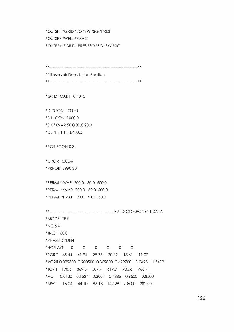
126
*OUTSRF *GRID *SO *SW *SG *PRES
*OUTSRF *WELL *PAVG
*OUTPRN *GRID *PRES *SO *SG *SW *SIG
**--------------------------------------------------------------------**
** Reservoir Description Section
**--------------------------------------------------------------------**
*GRID *CART 10 10 3
*DI *CON 1000.0
*DJ *CON 1000.0
*DK *KVAR 50.0 30.0 20.0
*DEPTH 1 1 1 8400.0
*POR *CON 0.3
*CPOR 5.0E-6
*PRPOR 3990.30
*PERMI *KVAR 200.0 50.0 500.0
*PERMJ *KVAR 200.0 50.0 500.0
*PERMK *KVAR 20.0 40.0 60.0
**--------------------------------------------------FLUID COMPONENT DATA
*MODEL *PR
*NC 6 6
*TRES 160.0
*PHASEID *DEN
*HCFLAG 0 0 0 0 0 0
*PCRIT 45.44 41.94 29.73 20.69 13.61 11.02
*VCRIT 0.099800 0.200500 0.369800 0.629700 1.0423 1.3412
*TCRIT 190.6 369.8 507.4 617.7 705.6 766.7
*AC 0.0130 0.1524 0.3007 0.4885 0.6500 0.8500
*MW 16.04 44.10 86.18 142.29 206.00 282.00
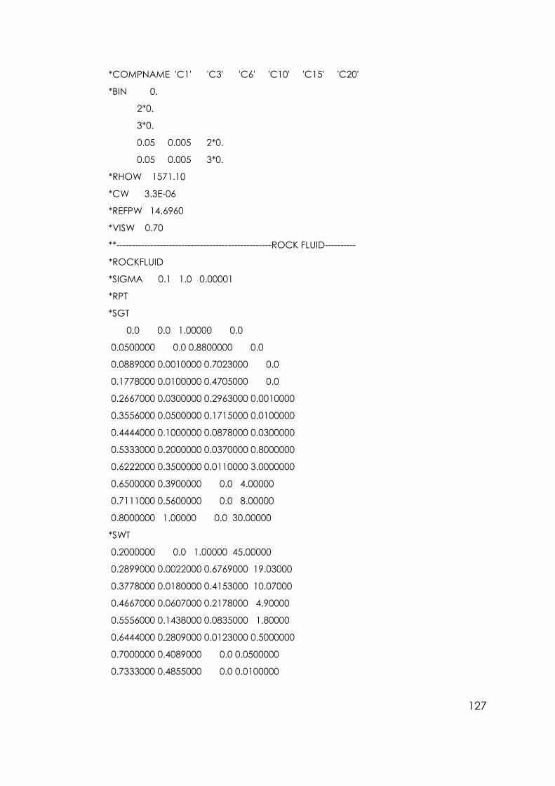
127
*COMPNAME 'C1' 'C3' 'C6' 'C10' 'C15' 'C20'
*BIN 0.
2*0.
3*0.
0.05 0.005 2*0.
0.05 0.005 3*0.
*RHOW 1571.10
*CW 3.3E-06
*REFPW 14.6960
*VISW 0.70
**--------------------------------------------------ROCK FLUID----------
*ROCKFLUID
*SIGMA 0.1 1.0 0.00001
*RPT
*SGT
0.0 0.0 1.00000 0.0
0.0500000 0.0 0.8800000 0.0
0.0889000 0.0010000 0.7023000 0.0
0.1778000 0.0100000 0.4705000 0.0
0.2667000 0.0300000 0.2963000 0.0010000
0.3556000 0.0500000 0.1715000 0.0100000
0.4444000 0.1000000 0.0878000 0.0300000
0.5333000 0.2000000 0.0370000 0.8000000
0.6222000 0.3500000 0.0110000 3.0000000
0.6500000 0.3900000 0.0 4.00000
0.7111000 0.5600000 0.0 8.00000
0.8000000 1.00000 0.0 30.00000
*SWT
0.2000000 0.0 1.00000 45.00000
0.2899000 0.0022000 0.6769000 19.03000
0.3778000 0.0180000 0.4153000 10.07000
0.4667000 0.0607000 0.2178000 4.90000
0.5556000 0.1438000 0.0835000 1.80000
0.6444000 0.2809000 0.0123000 0.5000000
0.7000000 0.4089000 0.0 0.0500000
0.7333000 0.4855000 0.0 0.0100000
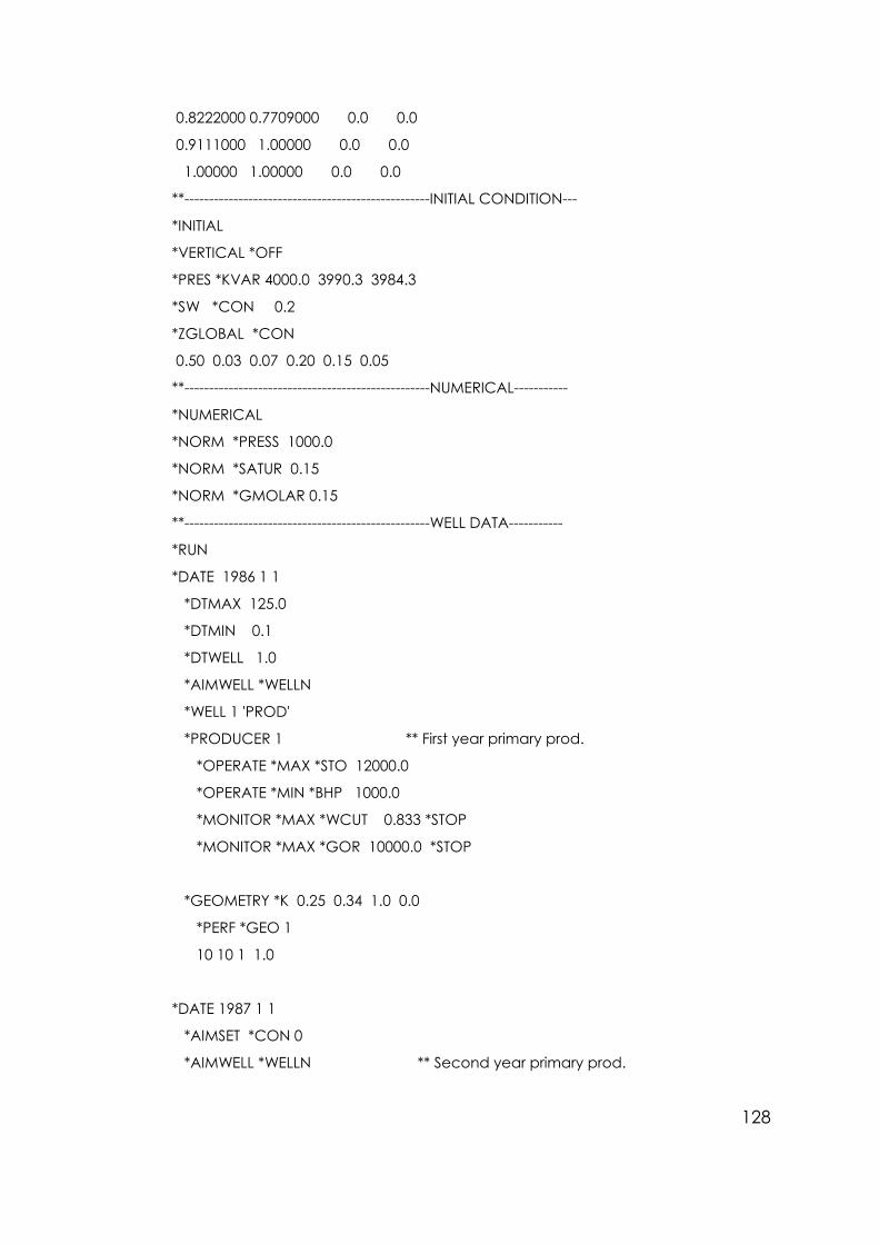
128
0.8222000 0.7709000 0.0 0.0
0.9111000 1.00000 0.0 0.0
1.00000 1.00000 0.0 0.0
**--------------------------------------------------INITIAL CONDITION---
*INITIAL
*VERTICAL *OFF
*PRES *KVAR 4000.0 3990.3 3984.3
*SW *CON 0.2
*ZGLOBAL *CON
0.50 0.03 0.07 0.20 0.15 0.05
**--------------------------------------------------NUMERICAL-----------
*NUMERICAL
*NORM *PRESS 1000.0
*NORM *SATUR 0.15
*NORM *GMOLAR 0.15
**--------------------------------------------------WELL DATA-----------
*RUN
*DATE 1986 1 1
*DTMAX 125.0
*DTMIN 0.1
*DTWELL 1.0
*AIMWELL *WELLN
*WELL 1 'PROD'
*PRODUCER 1 ** First year primary prod.
*OPERATE *MAX *STO 12000.0
*OPERATE *MIN *BHP 1000.0
*MONITOR *MAX *WCUT 0.833 *STOP
*MONITOR *MAX *GOR 10000.0 *STOP
*GEOMETRY *K 0.25 0.34 1.0 0.0
*PERF *GEO 1
10 10 1 1.0
*DATE 1987 1 1
*AIMSET *CON 0
*AIMWELL *WELLN ** Second year primary prod.

129
*DATE 1988 1 1
*DTWELL 2.0
*AIMSET *CON 0
*AIMWELL *WELLN
*WELL 2 'INJ-H2O'
*INJECTOR 2
*INCOMP *WATER ** Water injection
*OPERATE *MAX *STW 12000.0 ** WAG of 1 year cycle
*PERF *GEO 2
1 1 3 1.0
*WELL 3 'INJ-GAS'
*INJECTOR 3
*INCOMP *SOLVENT 0.77 0.20 0.03 0.0 0.0 0.0
*OPERATE *MAX *STG 1.20E+7
*PERF *GEO 3
1 1 3 1.0
*SHUTIN 3
*DATE 1989 1 1
*DTWELL 5.0
*SHUTIN 2
*OPEN 3 ** Solvent injection
*DATE 1990 1 1
*SHUTIN 3
*OPEN 2
*DATE 1991 1 1
*STOP