Embed Size (px)
Citation preview

GEOTHERMAL TRAINING PROGRAMME Reports 2008 Orkustofnun, Grensásvegur 9, Number 6 IS-108 Reykjavík, Iceland
CHARACTERIZATION OF THE HELLISHEIDI-THRENGSLI CO2 SEQUESTRATION TARGET AQUIFER BY TRACER TESTING
MSc thesis Department of Earth Sciences, Faculty of Science
University of Iceland
by
Mahnaz Rezvani Khalilabad SUNA – Renewable Energy Organization of Iran
Yadegare Emam Highway, Poonake Bakhtari Ave. Sharake Ghods, P.O. Box 14155-6398
Tehran IRAN
United Nations University Geothermal Training Programme
Reykjavík, Iceland Published in December 2008
ISBN 978-9979-68-252-3
ISSN 1670-7427

ii
This MSc thesis has also been published by the Faculty of Science – Department of Earth Sciences
University of Iceland

iii
INTRODUCTION
The Geothermal Training Programme of the United Nations University (UNU) has operated in Iceland since 1979 with six month annual courses for professionals from developing countries. The aim is to assist developing countries with significant geothermal potential to build up groups of specialists that cover most aspects of geothermal exploration and development. During 1979-2008, 402 scientists and engineers from 43 countries have completed the six month courses. They have come from Asia (44%), Africa (26%), Central America (15%), and Central and Eastern Europe (15%). There is a steady flow of requests from all over the world for the six month training and we can only meet a portion of the requests. Most of the trainees are awarded UNU Fellowships financed by the UNU and the Government of Iceland. Candidates for the six month specialized training must have at least a BSc degree and a minimum of one year practical experience in geothermal work in their home countries prior to the training. Many of our trainees have already completed their MSc or PhD degrees when they come to Iceland, but several excellent students have made requests to come again to Iceland for a higher academic degree. In 1999, it was decided to start admitting UNU Fellows to continue their studies and study for MSc degrees in geothermal science or engineering in co-operation with the University of Iceland. An agreement to this effect was signed with the University of Iceland. The six month studies at the UNU Geothermal Training Programme form a part of the graduate programme. Six UNU-GTP MSc Fellows completed their MSc degree in 2008, the biggest group to date. It is a pleasure to introduce the second woman and the sixteenth UNU Fellow to complete the MSc studies at the University of Iceland under the co-operation agreement. Ms. Mahnaz Rezvani Khalilabad, BSc in Geology from the Shahid Beheshti University in Iran, of SUNA – Renewable Energy Organization of Iran, completed the six month specialized training in Reservoir Engineering at the UNU Geothermal Training Programme in October 2003. Her research report was entitled “Reservoir parameters for well HE-5, Hellisheidi, geothermal field, SW-Iceland”. Three years later, in September 2006, she came back to Iceland for MSc studies in Reservoir Engineering and Environmental Sciences at the Department of Earth Sciences within the Faculty of Science of the University of Iceland. In September 2008, she defended her MSc thesis presented here, entitled “Characterization of the Hellisheidi-Threngsli CO2 sequestration target aquifer by tracer testing”. Her studies in Iceland were financed by a fellowship from the Government of Iceland through the UNU Geothermal Training Programme. We congratulate Ms. Mahnaz Rezvani Khalilabad on her achievements and wish her all the best in her PhD studies in Canada and for the future. We thank the Department of Earth Sciences of the University of Iceland for the co-operation, and her supervisors for the dedication. Finally, I would like to mention that Mahnaz’ MSc thesis with the figures in colour is available for downloading on our website at page www.unugtp.is/yearbook/2008. With warmest wishes from Iceland, Ingvar B. Fridleifsson, director United Nations University Geothermal Training Programme

iv
ACKNOWLEDGEMENT
This study was sponsored by the Government of Iceland, through the United Nations University Geothermal Training Programme. The associated field research operation was funded by Reykjavik Energy through the CarbFix program. I would like to express my heart-felt gratitude to Dr. Gudni Axelsson and Dr. Sigurdur Reynir Gíslason, my advisors, for their very good teaching and support. I would also like to thank friends and colleagues at Reykjavik Energy and ISOR (Iceland GeoSurvey) for the project organization, field operation and keen assistance during data collection, especially Hólmfrídur Sigurdardóttir, Grímur Björnsson, Magnús Ólafsson, Kristján Hrafn Sigurdsson, Grétar Ívarsson, Einar Gunnlaugsson, Thórólfur H. Hafstad, and Benedikt Steingrímsson. I appreciate Dr. Ingvar Birgir Fridleifsson, Director of the UNU-GTP, and Mr. Lúdvík S. Georgsson, Deputy Director, for their continuous support and assistance. This work is dedicated to my family for their encouraging efforts and full support during the study, especially my beloved husband Mr. Abolfazl Asghari and our son Aryan.
v
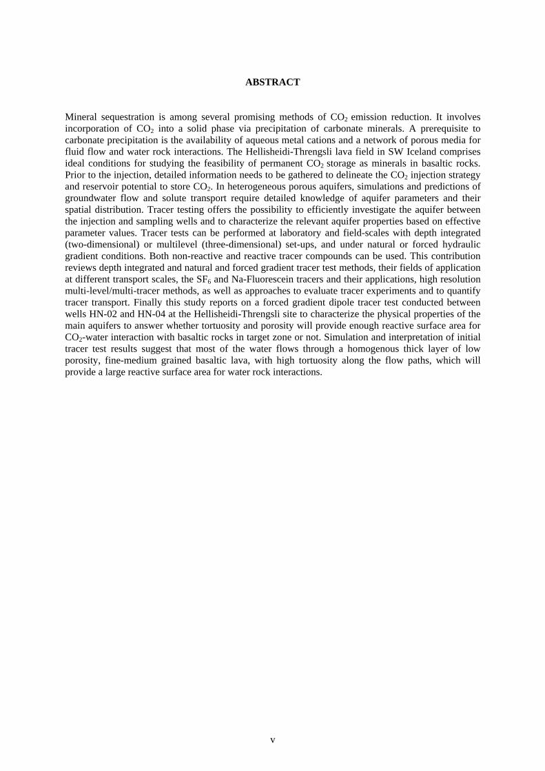
ABSTRACT
Mineral sequestration is among several promising methods of CO2 emission reduction. It involves incorporation of CO2 into a solid phase via precipitation of carbonate minerals. A prerequisite to carbonate precipitation is the availability of aqueous metal cations and a network of porous media for fluid flow and water rock interactions. The Hellisheidi-Threngsli lava field in SW Iceland comprises ideal conditions for studying the feasibility of permanent CO2 storage as minerals in basaltic rocks. Prior to the injection, detailed information needs to be gathered to delineate the CO2 injection strategy and reservoir potential to store CO2. In heterogeneous porous aquifers, simulations and predictions of groundwater flow and solute transport require detailed knowledge of aquifer parameters and their spatial distribution. Tracer testing offers the possibility to efficiently investigate the aquifer between the injection and sampling wells and to characterize the relevant aquifer properties based on effective parameter values. Tracer tests can be performed at laboratory and field-scales with depth integrated (two-dimensional) or multilevel (three-dimensional) set-ups, and under natural or forced hydraulic gradient conditions. Both non-reactive and reactive tracer compounds can be used. This contribution reviews depth integrated and natural and forced gradient tracer test methods, their fields of application at different transport scales, the SF6 and Na-Fluorescein tracers and their applications, high resolution multi-level/multi-tracer methods, as well as approaches to evaluate tracer experiments and to quantify tracer transport. Finally this study reports on a forced gradient dipole tracer test conducted between wells HN-02 and HN-04 at the Hellisheidi-Threngsli site to characterize the physical properties of the main aquifers to answer whether tortuosity and porosity will provide enough reactive surface area for CO2-water interaction with basaltic rocks in target zone or not. Simulation and interpretation of initial tracer test results suggest that most of the water flows through a homogenous thick layer of low porosity, fine-medium grained basaltic lava, with high tortuosity along the flow paths, which will provide a large reactive surface area for water rock interactions.

vi
TABLE OF CONTENTS Page 1. INTRODUCTION ......................................................................................................................... 1 1.1 Project statement – CO2 sequestration ................................................................................. 1 1.2 Research objectives of thesis project within the CarbFix project; aquifer characterization using tracer test technique ........................................................ 2 2. BACKGROUND ........................................................................................................................... 3 2.1 Flowing fluid through an aquifer ......................................................................................... 3 2.2 Concepts and definitions of fluid transport mechanics ........................................................ 4 2.3 Fickian diffusion equation ................................................................................................... 5 2.4 The advective diffusion equation ......................................................................................... 7 2.5 The Peclet number ............................................................................................................... 8 2.6 The dispersion equation ....................................................................................................... 8 2.6.1 Effective diffusion coefficient in porous media ................................................... 9 2.6.2 Mechanical dispersion in ground water .............................................................. 10 3. AQUIFER CHARACTERIZATION WITH TRACER TEST TECHNIQUE ............................. 11 3.1 Tracer test technique .......................................................................................................... 11 3.2 Aquifer heterogeneity ........................................................................................................ 11 3.3 Scale and implications of tracer testing ............................................................................. 12 3.4 Tracer test strategy ............................................................................................................. 13 3.4.1 Tracer test gradient condition ............................................................................. 13 3.4.2 Natural gradient tracer tests ................................................................................ 14 3.4.3 Forced gradient tracer tests ................................................................................. 14 3.4.4 Tracer injection methods .................................................................................... 15 3.4.5 Multi tracer approach and DNA tracers ............................................................. 16 3.4.6 High resolution multilevel- multi-tracer sampling and concentration measuring equipment .............................................................. 16 3.4.7 Multi-tracer forced gradient transport experiments, investigation of physical and hydro-geochemical aquifer properties ............ 17 3.5 Tracer material ................................................................................................................... 18 3.5.1 Tracer selection .................................................................................................. 18 3.5.2 Na-fluorescein .................................................................................................... 18 3.5.3 SF6 ...................................................................................................................... 19 3.5.4 Tracer mass and sample collection frequency .................................................... 20 4. THE HELLISHEIDI–THRENGSLI SITE - NATURAL CO2 INJECTION LABORATORY ... 22 4.1 The Hellisheidi–Threngsli CO2 injection site .................................................................... 24 4.2 Porosity and permeability structure in the Hellisheidi-Threngsli area .............................. 25 4.3 Target wells ....................................................................................................................... 27 4.3.1 Well HN-02 ........................................................................................................ 27 4.3.2 Well HN-04 ........................................................................................................ 29 4.4 Governing flow direction and velocity in the intermediate ground water system ............. 30 4.5 Execution of the initial short tracer test ............................................................................. 31 4.6 Theoretical solution adapted for the Hellisheidi-Threngsli short tracer test ...................... 32 4.6.1 Required mass of tracer ...................................................................................... 33 4.6.2 Sample collection frequency .............................................................................. 33 4.6.3 Sample analysis and breakthrough curve ........................................................... 34 4.7 Tracer test breakthrough curve and data simulation .......................................................... 35 4.8 Simulation result discussions ............................................................................................. 37 5. CONCLUDING REMARKS ....................................................................................................... 38

vii
Page LIST OF SYMBOLS ............................................................................................................................ 39 REFERENCES ............................................................................................................................ 40 LIST OF FIGURES 1. Plume created by instantaneous source in flow field ..................................................................... 5 2. Differential control volume for derivation of diffusion equation .................................................. 6 3. Dispersion in ground water ............................................................................................................ 9 4. Tortuosity arises because of longer flow-paths .............................................................................. 9 5. Causes of mechanical dispersion on different scales. .................................................................. 10 6. Stepwise flow chart of a tracer test .............................................................................................. 12 7. Multi level sampling within pumping wells. ................................................................................ 17 8. Forced gradient multilevel–multitracer approach. ....................................................................... 17 9. Atmospheric concentration of the SF6 in the last 100 years used to date the groundwater. ........ 20 10. Aerial photo of the Hellisheidi-Threngsli area ............................................................................. 22 11. Map of the Hellisheidi–Threngsli area, in the SW-part of the Hengill region. ............................ 23 12. Three-dimensional sketch of the Hellisheidi–Threngsli CO2 injection target zone ..................... 24 13. NE-SW cross section through the Hellisheidi-Threngsli field. .................................................... 25 14 Temperature profiles for well HN-02 .......................................................................................... 27 15. Temperature changes of drilling fluid before injection and after circulation during drilling of well HN-02 ................................................................................................. 28 16. Lithological log and possible aquifer locations in well HN-02 for the first 1000 m depth .......... 28 17. The design of well HN-04, measured lateral deviation towards west and numerical values for true vertical depth and lateral deviation. ........................................ 29 18. Lithological log and location of possible aquifers in ................................................................... 29 19. Available temperature logs from well HN-04 .............................................................................. 30 20. Surface set-up for tracer test between wells HN-02 and HN-04. ................................................. 32 21. Theoretical tracer recovery curves ............................................................................................... 34 22. Sampling bottle for Na-Fluorescein sampling and sanitary gloves. ............................................. 34 23. Turner Designs TD-700 Fluorimeter and calibration process. ..................................................... 35 24. The tracer test recovery results for well HN-04 ........................................................................... 35 25. Observed and simulated Na-fluorescein recovery in well HN-04 ............................................... 36 LIST OF TABLES 1. Geological features contributing to non-idealities in porous medium ......................................... 10 2. The advantages and disadvantages of the NGTT and FGTT methods......................................... 14 3. Water level measurements and elevation of wells HN-01, HK-31 and HK-26. .......................... 31 4. Model parameters used to simulate the tracer recovery with 3 channels ..................................... 36

viii

1
1. INTRODUCTION Urgent efforts need to be considered to meet the increasingly serious environmental and economic threats of climate change due to CO2 emission in the global energy supply (REN21, 2008). Efforts to reduce CO2 emissions in a Carbon-Constrained World cites an “emerging consensus” in both the scientific and political communities for a global warming limit of 2°C above pre-industrial levels. This goal can only be reached with major long-term emission reductions through different and combined options. These include larger renewable energy markets, efficiency improvements in conventional energy sectors and providing fossil fuels that are much cleaner than those on which the world’s US$60 trillion economy currently depends. Moreover, there should be a major step toward mitigating the effect of existing CO2 and ongoing facilities with large CO2 emission volumes. Some ongoing projects have already started to apply different ways of CO2 storage in various underground aquifers. These recent efforts in carbon capture could be accelerated by global and national driving forces, as has happened in many green energy strategy cases. Many renewable energy technologies have moved from being a passion for the dedicated few to a major economic sector attracting large industrial companies and financial institutions (Ragnarsson, 2003). However, basic policy questions remain, including the need to ensure technical progress, overcome implementation barriers, and accelerate the shift to new ideas. The energy sector has already taken steps to reduce CO2 emissions, in particular through utilization of renewable energy sources, as mentioned above, but major steps need to be taken to reduce or capture the CO2 emissions from conventional mobile sources and stationary sources. Scientists at the University of Iceland, Reykjavik Energy in Iceland, Columbia University in the USA, and CNRS in Toulouse, France, have taken an initiative by setting up a co-operative research project, CarbFix, to optimize methods for storing CO2 in basaltic rocks. CO2 will be provided by gas emitted from the Hellisheidi geothermal power plant located close to the targeted geological aquifer in the Hellisheidi-Threngsli area in SW-Iceland. The CarbFix project was formally launched in September 2007 and will last for 3-5 years. The schedule is optimistic and the plan is to start injection of CO2 from the Hellisheidi geothermal plant into basaltic bedrock of the Threngsli lava field in early 2009. 1.1 Project statement – CO2 sequestration CO2 emission and its effect on global warming is the most controversial issue in the scientific world today. In an attempt to reduce, or at least to slow down the increase in atmospheric CO2, a number of initiative methods have been suggested over the last few years. Geologic sequestration involves the injection of CO2 into the subsurface, typically into brine filled aquifers or in depleted oil field reservoirs (Holloway, 1997). During geologic sequestration, CO2 is stored in one of three ways, via hydrodynamics, solubility, or mineral trapping (Hitchen, 1996). Hydrodynamic trapping involves the storage of CO2 as a gas or supercritical fluid beneath a low permeability cap rock. Solubility trapping involves the dissolution of CO2 into a fluid phase, including both aqueous brines and oil. Mineral trapping involves incorporation of CO2 into a solid phase, for example, via the precipitation of carbonate minerals or its adsorption onto coal. Many have referred to mineral trapping as permanent CO2 sequestration because of the ability of many carbonate phases to remain stable for geologically significant time frames (e.g. Bachu et al., 1995 and Perkins and Gunter, 1995). A prerequisite to carbonate precipitation is the availability of aqueous divalent metal cations, originating from non-carbonate minerals, which can combine with dissolved CO2. One potential source of these cations is the dissolution of metal bearing silicate rocks like basalt. Moreover, a large potential of storage capacity in basalt porous media will provide tortuosity of flow paths and a great deal of potential reactive surface area for water rock interaction and consequently carbonate precipitation. Risks are nevertheless present. CO2 can leak from the subsurface before carbonate precipitation, returning some of the injected CO2 to the atmosphere. Furthermore, precipitation of secondary minerals to close to the injection site can lead to lower permeability arresting further CO2 injection (Oelkers and Schott, 2005).

2
In the CarbFix project the investigations are aimed at carrying out experiments in a natural “laboratory” in basaltic formations in SW-Iceland to study the possibility of permanent CO2 sequestration. CO2 will be provided by the Hellisheidi geothermal power plant located close to the targeted geological site. It will be dissolved in water at elevated pressure at about 25°C and injected into the basaltic bedrock at a depth of 400 to 800 m, i.e. the so called “target zone”. The site comprises ideal conditions for studying the feasibility of permanent CO2 storage as minerals in basaltic rocks. A glassy basaltic formation, referred to as hyaloclastite, would provide the metal bearing silicates providing divalent cations for interaction. Horizontal lava flows are cut by a number of shallow and deep wells, which have provided a great deal of geological and hydrogeological information through well logging data. Existing information will facilitate the injection experiment as well as monitoring of the changes in the target zone during CO2 injection. This project will tackle the risks involved through natural laboratory experiments, which makes it a unique project among other CO2 capture and storage studies 1.2 Research objectives of thesis project within the CarbFix project; aquifer characterization using tracer test technique Based on character of the porous media, fluid could be extracted or transported. Petrophysical characterization of the target aquifers determines the fate of CO2 storage and the available residence time for water rock interactions. Knowledge of pore size and petrophysical characteristics is essential for defining the CO2 injection strategy, including the amount of CO2 to be injected. A clear picture of the host formation is necessary; both of the macroscopic assemblage of geological layers and microstructures inside the layers. Macro scale effects like regional groundwater flow in the area could sweep away the injected CO2 for tens of kilometres. This has the benefit that a large volume of rock will be available for CO2 precipitation but it may drive the CO2 to unfavourable formations rather than the target formation. To avoid such risks, governing flow in the aquifers and flow velocities have to be precisely defined. To investigate the host formation characteristics a number of onsite tests can be performed. Regional geophysical studies and well testing with more local focuses are among the possible investigation tools. Tracer test techniques are the most effective and descriptive indirect tools available to investigate the petrophysical parameters of the target geological setting (Kass, 1998). Tracer tests will provide valuable information on porosity, type of flow path interconnection and governance of flow in the test scale area. To achieve such goals during the lifetime of the CarbFix project a number of tracer tests have been planned. This includes a short tracer test during the pre-feasibility stage of CO2 injection, the results of which will help to plan and conduct a follow-up large-scale tracer test. A large-scale tracer test is designed to establish base-line conditions of the target formation. For the initial short tracer test in the target block of Hellisheidi–Threngsli wells HN-02 and HN-04 were selected. The results have been evaluated to assess the type of permeability and amount of porosity in the target zone, which refers to the 400-800 m depth section consisting mostly of basaltic formations. This basaltic formation is the ideal aquifer for the required water–rock interaction for CO2 sequestration. This thesis will first review the theoretical background for tracer test execution and interpretation. It covers the overall description of tracer tests and their implications based on the scale of a study and the strategy of executing tracer tests in different fields. Different tracer test types will be discussed with respect to gradient conditions, tracer materials and functions. Multi tracer approaches and high-resolution multi-level/multi-tracer tests with recent technological advances will be discussed. This will be followed by a description of the details of the short tracer experiment in Hellisheidi-Threngsli as well as a description of field conditions. The tracer test design, execution, data gathering, model simulation and interpretation will, in particular, be discussed. Finally, the thesis will be concluded by a discussion of the reactive surface area available in the target zone, based on the tracer test results, and with remarks on the follow-up large-scale tracer test. The short tracer test will try to answer; will tortuosity and porosity provide enough reactive surface area for CO2-water interaction with basaltic rocks in the target zone or not?

3
2. BACKGROUND Rain fall and snow melt can flow into rivers and streams, return to the atmosphere by evaporation or transpiration, or seep into ground water to become part of the subsurface or ground, water. A so-called aquifer is a saturated geologic layer that is permeable enough to allow water to flow fairly easily through it. An aquifer sits on top of a confining bed or, as it is sometimes called, an aquitard or an aquiclude, which is a relatively impermeable layer that greatly, restricts the movement of groundwater. The two terms, aquifer and confining bed, are not precisely defined and are often used in a relative sense (Masters and Wendell, 2007). In this chapter, we will cover the ground water movement processes in detail and establish the background necessary to tackle the goal of this study. 2.1 Flowing fluid through an aquifer The amount of water that can be stored in a saturated aquifer depends on the porosity of the formation or rock that makes up the aquifer. Porosity φ is defined to be the ratio of the volume of voids to total volume of material:
( )solidofvolumeTotal
voidofVolumePorosity =ϕ (1)
While porosity describes the water-bearing capacity of the geologic formation, it is not a good indicator of the total amount of water that can be removed from a given formation. The volume of water that can actually be drained from an unconfined aquifer per unite area per unite decline in the water table (or pressure) is called specific yield, or effective porosity (Masters and Wendell, 2007). In an unconfined aquifer, the slope of the water table, measured in the direction of the steepest rate of change, is called the hydraulic gradient. It is important because ground water flow is in the direction of the gradient and at a rate proportional to the gradient. The French hydraulic engineer Henri Darcy formulated the basic equation governing ground water flow in 1856, based on laboratory experiments in which he studied the flow of water through sand filters (Bedient et al., 1994). Darcy concluded that flow rate Q is proportional to the cross sectional area times the hydraulic gradient, ∂h/∂L. Equation 2, known as Darcy’s law, describes fluid flow through porous media: ( )L
hAKQ ∂∂= (2)
where Q = Flow rate (m3/s) K = Hydraulic Conductivity, or coefficient of permeability (m/s) A = Cross-sectional area (m2) ∂h/∂L = The hydraulic gradient Aquifers that have the same hydraulic conductivity throughout are said to be homogeneous, whereas those in which hydraulic conductivity differs from place to place are heterogeneous. Not only may hydraulic conductivity vary from place to place within the aquifer, but it may also depend on the direction of flow. It is common, for example, to have higher hydraulic conductivities in the horizontal direction than in the vertical. Aquifers that have the same hydraulic conductivity in any flow direction are said to be isotropic, whereas those in which conductivity depends on direction are anisotropic. Although it is mathematically convenient to assume that aquifers are both homogeneous and isotropic, they rarely, are so. It is often important to estimate the rate at which groundwater is moving through an aquifer, especially when transport processes within the aquifer are being studied. If we combine the relationship between flow rate, average velocity, and cross-sectional area: Q=Au (3)

4
With Darcy’s law, we can solve for velocity:
( )( )LhKu
ALhAKuAQu
∂∂=∂∂=
= (4)
The velocity given in Equation 4 is known as the Darcy velocity. It is not a real velocity in that, in essence, it assumes that the full cross-sectional area A is available for water to flow through. Since much of the cross-sectional area is made up of solids, the actual area through which all the flow takes place is much smaller, and as a result, the real ground water velocity is considerably faster than the Darcy velocity. It means that average linear velocity can be determined by: ϕuPorosityvelocityDarcyu ==, (5) ( ) ϕLhKu ∂∂=, (6) 2.2 Concepts and definitions of fluid transport mechanics Studies of fluid mechanical transport deal with the fate and transport of substances through the hydrosphere and atmosphere at a local or regional scale (up to 100 km). In layman terms environmental fluid mechanics studies how fluids move substances through the natural environment as they are also transformed. In general, the substances we may be interested in are mass, momentum or heat. More specifically, mass can represent any of a wide variety of passive and reactive chemicals, such as dissolved oxygen, salinity, heavy metals, nutrients, artificial tracers and many others. Stated simply, fluid transport mechanics is the study of natural processes that change concentrations. These processes can be categorized into two broad groups: transport and transformation. Transport refers to those processes which move substances through the hydrosphere and atmosphere by physical means. The three primary modes of transport in environmental fluid mechanics are diffusion (transport associated with random motions within a fluid), advection (transport associated with the flow of a fluid) and dispersion, which is the dominant phenomenon in the media with different shear stresses in the cross section due to different flow paths or velocity. The second process, transformation, refers to those processes that change a substance of interest into another substance. The two primary modes of transformation are physical (transformations caused by physical laws, such as radioactive decay) and chemical (transformations caused by chemical or biological reactions, such as dissolution and respiration (Socolofsky and Jirka, 2005). In ground water environments, the most important transport processes are advection and dispersion, whereas transformation includes all categories of chemical, nuclear and biological processes. We can list acid-base reactions, solution, volatilization and precipitation, complexation, sorption reactions, oxidation-reduction reactions, hydrolysis reactions and isotopic reactions (Domenico and Schwartz, 1990). In advection, the mean linear fluid velocity is the governing force moving the mass along the flow path and mass spreading in steady state systems more or less defined by path lines, even in relatively complex flow system. Because advection is the dominant transport process, knowledge of ground water flow patterns provides the key to interpreting the pattern of contaminant migration in such systems (Domenico and Schwartz, 1990). A second process that causes a chemical component plume to spread out is dispersion. Since such a plume follows irregular pathways as it moves, some through large pore spaces in which portion of the plume can move quickly, while other portions of the plume have to force their way through more confining voids, there will be a difference in speed of an advancing plume that tends to cause the plume to spread out.

5
Although the most effective processes are advection and dispersion we should keep in mind that when there is a difference in concentration of a solute in groundwater, molecular diffusion will tend to cause movement from regions of high concentration to regions where the concentration is lower. That is, even in absence of ground water movement, a blob of contaminant will tend to diffuse in all directions, blurring the boundary between it and the surrounding groundwater. Since diffusion and dispersion both tend to smear the edges of the plume, they are sometimes linked together and simply referred to as hydrodynamic dispersion. A concentration cloud spreads out as it moves; it does not arrive all at the same time at a given location down gradient. As the plume moves down gradient, dispersion causes the plume to spread in the longitudinal, as well as horizontal, directions (Figure 1). Another concept that we have to keep in mind is that chemicals/contaminants may not move at the same speed as the ground water. As contaminants move through an aquifer, solids along the way absorb some, and some chemicals are adsorbed (that is adhered to the surface of particles). The general term sorption applies to both processes. Sorption of material will make a phenomenon, which is called retardation (R). 2.3 Fickian diffusion equation As mentioned, a fundamental transport process in environmental fluid mechanics is diffusion. Diffusion has two primary properties: it is random in nature, and transport is from regions of high concentration to regions of low concentration, with an equilibrium state of uniform concentration. High concentration tends to spread into regions of low concentration under the action of diffusion. The diffusion coefficient, D, is the intensity, energy and freedom of motion, of this Brownian motion. Thus, D depends on the phase (solid, liquid or gas), temperature, and molecule size. For dilute solutes in water, D is generally of order 2 x10⁻⁹ m2/s, whereas, for dispersed gases in air, D is of order 2 x10⁻⁵ m2/s, with a difference in magnitude of 104. With the constant, which we call the diffusion coefficient, D, the diffusive flux equation, defined by Equation 7, predicts this spreading-out process (Fischer et al., 1979): xCDq x ∂∂−= (7) Generalizing to three dimensions, we can write the diffusive flux vector at a point as in Equation 8:
ixCDq
CDqzC
yC
xCDq
∂∂
−=
∇−=
⎟⎟⎠
⎞⎜⎜⎝
⎛∂∂
∂∂
∂∂
−= ,,
(8)
Diffusion processes that obey this relationship are called Fickian diffusion, and Equation 8 is called Fick’s law. Although Fick’s law gives us an expression for the flux of mass due to the process of
FIGURE 1: An instantaneous (pulse) source in a flow field creates a plume that spreads as it moves down
gradient: (a) in one dimension, (b) in two dimensions, darker colours mean higher concentrations
(Bedient et al., 1994)
6
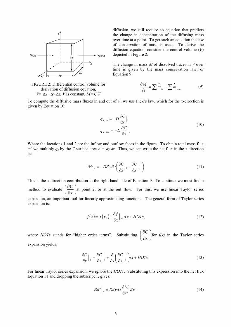
diffusion, we still require an equation that predicts the change in concentration of the diffusing mass over time at a point. To get such an equation the law of conservation of mass is used. To derive the diffusion equation, consider the control volume (V) depicted in Figure 2. The change in mass M of dissolved tracer in V over time is given by the mass conservation law, or Equation 9:
⋅
••
∑∑ −=∂∂
outinmm
tM (9)
To compute the diffusive mass fluxes in and out of V, we use Fick’s law, which for the x-direction is given by Equation 10:
2,
1,
xCDq
xCDq
outx
inx
∂∂
−=
∂∂
−= (10)
Where the locations 1 and 2 are the inflow and outflow faces in the figure. To obtain total mass flux m˙ we multiply qx by the V surface area A = δy.δz. Thus, we can write the net flux in the x-direction as:
⎟⎠⎞
⎜⎝⎛
∂∂
−∂∂
−=21 x
CxCzyDm x δδδ & (11)
This is the x-direction contribution to the right-hand-side of Equation 9. To continue we must find a
method to evaluate ⎟⎠⎞
⎜⎝⎛∂∂
xC
at point 2, or at the out flow. For this, we use linear Taylor series
expansion, an important tool for linearly approximating functions. The general form of Taylor series expansion is:
( ) ( ) ,
00 HOTsxxfxfxf x +
∂∂
+= δ (12)
where HOTs stands for “higher order terms”. Substituting ⎟⎠⎞
⎜⎝⎛∂∂
xC
for f(x) in the Taylor series
expansion yields:
⋅+⎟
⎠⎞
⎜⎝⎛∂∂
∂∂
+∂∂
=∂∂ HOTsx
xC
xxC
xC δ
112 (13)
For linear Taylor series expansion, we ignore the HOTs. Substituting this expression into the net flux Equation 11 and dropping the subscript 1, gives:
⋅∂∂
=• xxCzyDm x δδδδ 2
2
(14)
FIGURE 2: Differential control volume for derivation of diffusion equation,
V= ∆x· ∆y·∆z, V is constant, M =C·V

7
Similarly, in the y- and z-directions, the net fluxes through the control volume are:
z
zCzxDm
yyCzxDm
z
y
δδδδ
δδδδ
2
2
2
2
∂∂
=
∂∂
=
•
•
(15)
Before substituting these results into Equation 9, we also convert M to concentration by recognizing
M = C·δx·δy·δz. After substitution of the concentration C and net fluxes, δ•
m into Equation 9, we obtain the three-dimensional diffusion equation (in various types of notation). This is the fundamental equation in environmental fluid mechanics:
2
2
2
2
2
2
2
2
ixCD
tC
CDtC
zC
yC
xCD
tC
∂
∂=
∂∂
∇=∂∂
⎟⎟⎠
⎞⎜⎜⎝
⎛
∂∂
+∂∂
+∂∂
=∂∂
(16)
In the one-dimensional case, concentration gradients in the y- and z-direction are zero, and we have the one-dimensional diffusion equation:
.2
2
xCD
tC
∂∂
=∂∂ (17)
Solution of Equation 17 is discussed in many textbooks (e.g. Fischer et al., 1979; Socolofsky and Jirka, 2005; Masters and Wendell, 2007). By generalizing the solution Equation 18 is obtained, which has been derived using the separation of variables method. This solution will be used throughout this text:
⎟⎟⎠
⎞⎜⎜⎝
⎛−−−=
tDz
tDy
tDx
tDDDMtzyxC
zyxzyx 444exp
44),,,(
222
ππ (18)
2.4 The advective diffusion equation In nature, solute transport in fluids occurs through the combination of advection and diffusion. If we open a valve and allow water to flow in a pipe, we expect the centre of mass of the solute-chemical cloud to move with mean flow velocity in the pipe. If we move our frame of reference with that mean velocity and assume the non-viscous case, then we expect the solution to look same as before. This new reference frame is: )( ,
0 tuxx +−=η (19) Where η is the moving reference frame spatial coordinate, x0 is the injection point of the tracer, u is the mean flow velocity, and u’t is the distance travelled by the centre of mass of the cloud in time t. If we substitute η for x in our solution for a point source in stagnant conditions, we obtain for one-dimensional flow:

8
( )( )⎟⎟
⎠
⎞
⎜⎜
⎝
⎛ +−−=
Dttuxx
DtAMtxC
4exp
4),(
2,0
π (20)
To test whether this solution is correct, we need to derive a general equation for advective diffusion and compare its solution (e.g. Fischer et al., 1979, Socolofsky and Jirka, 2005, Masters and Wendell, 2007). 2.5 The Peclet number If the cross-flow (advection) is strong (larger u) the chemical-tracer cloud has less time to spread out and is relatively narrow as time t progresses. Conversely, if diffusion is strong (larger D) the cloud spreads out more with time. Thus, we see that diffusion versus advection dominance is a function of t, D, and u and we express this property through the non-dimensional Peclet number (Socolofsky and Jirka, 2005):
2,tu
DPe = (21)
or for a given downstream location given by L = u,t :
Lu
DPe ,= (22)
For Pe >> 1, diffusion is dominant and the cloud spreads out faster than it moves downstream; for Pe << 1, advection is dominant and the cloud moves downstream faster than it spreads out. It is important to note that the Peclet number is dependent on our zone of interest: for “large” times or distances, the Peclet number is small and advection dominates. 2.6 The dispersion equation A host of processes leads to a non-uniform velocity field, which allows the mass to spread through a much larger area up to the observation point rather than by molecular diffusion and advection alone. In this section, we are not going to formally derive the equations for non-uniform velocity fields to demonstrate their effects on the size of the zone of spreading. However, by either considering the effect of a random, turbulent velocity field or combined effects of diffusion (molecular or turbulent) with a shear velocity profile to develop equations for dispersion, the resulting equations retain their previous form. With just having the dispersion coefficients due to turbulent (Dt) orders of magnitude greater than the Molecular diffusion coefficients (Dm)(e.g. Fischer et al., 1979, Socolofsky and Jirka, 2005):
⎟⎟⎠
⎞⎜⎜⎝
⎛∂∂
∂∂
+⎟⎟⎠
⎞⎜⎜⎝
⎛∂∂
∂∂
=∂∂
+∂∂
im
iit
iii x
CDxx
CDxx
CutC (23)
As mentioned, Dt is the dispersion coefficient, which is usually much greater than the molecular diffusion coefficient Dm; thus in Equation 23 the final term is typically neglected. In groundwater, dispersion is the most important process to spread mass beyond the region it normally would occupy due to advection alone. Non uniform velocity distribution will make the dispersion effect the governing force to drive the contaminant-tracer spreading far beyond the flow paths (Figure 3).

9
Some of the mass moves in an advective front, which is defined as the product of the average linear velocity and time since displacement first started. Gradually a zone of mixing develops around the advective front leaving behind some tracer due to dispersion. More formally called hydrodynamic dispersion, it occurs because of two different process, diffusion and mechanical dispersion. These two contributions to hydrodynamic dispersion are represented mathematically as:
∗+= mLh DDD (24)
where Dh is the Coefficient of Hydrodynamic Dispersion, DL is the Coefficient of Mechanical Dispersion, and ∗
mD is the Effective Diffusion Coefficient. Now we describe the process of dispersion in ground water in more detail as follows. 2.6.1 Effective diffusion coefficient in porous media Molecular diffusion originates in mixing caused by random molecular motions due to thermal kinetic energy of solute. The diffusion coefficient in a porous medium is smaller than in pure liquids primarily because collision with the solids of the medium, hinder diffusion. In a porous medium, diffusion takes place in a liquid phase enclosed by a porous solid. Averaging techniques provide the following rigorous statement for Fick’s law in the fluid phase of porous sediments (Domenico et al., 1990):
( )⎥⎦
⎤⎢⎣
⎡+
∂∂
−= ,.
uxCDq mx
τϕ (25)
Here qx is a chemical mass flux, with the negative sign indicating that the transport is in direction of decreasing concentration, Dm is the molecular diffusion coefficient in a fluid environment, C is the concentration, φ porosity, τ is tortuosity defined as the ratio of the length of a flow channel for a fluid particle (Le) to the length of a porous medium sample (L) and u, is mean velocity (Figure 4).
Chemical molecular diffusion coefficient must be corrected to account for tortuosity and porosity. Effective diffusion coefficient in porous media increases with increasing porosity and decreases with increasing path length ratio. Effective diffusion coefficient is directly related to porosity and tortuosity:
mm DD
τϕ
∝∗ (26)
FIGURE 4: Tortuosity arises because of flow-paths longer than the most direct path
FIGURE 3: Dispersion in ground water due to non-uniform velocity distribution and different flow paths

10
2.6.2 Mechanical dispersion in ground water In mechanical dispersion, mixing occurs because of local variation in velocity around some mean velocity of flow. Thus, mechanical dispersion is an advective process and not a chemical one. The main cause of the variability in the direction and rate of transport are the porous medium non-idealities. The most important variable in this respect is effective porosity. Water travels at different speeds in individual pore channels, due to shear in contact with grains. The shear originating in the throat makes different velocity at a micro scale. On the other hand the different flow paths, because of differences in surface area and roughness relative to the volume of water in individual pore channels, make some channels are easier to flow through than others. Figure 5 shows the effect mentioned on different scales. In Table 1 some of the geological features that produce non-idealities based on scale are classified. The impression that the table should leave is that non-idealities can exist on a variety of scales ranging from microscopic to megascopic, to an even larger scale involving groups of formations. This effect can be observed in 3 dimensions. But obviously because of the mean velocity the longitudinal mechanical dispersion is much greater than that in transverse directions. Longitudinal mechanical dispersion coefficient (DL) is written as:
,. uD LL α= (27)
where αL = The longitudinal dispersivity, a function of the medium; u, = The average linear velocity or water speed in the direction of flow. Longitudinal dispersivity has the unit of length, and like hydraulic conductivity is a characteristic property of a medium. In practice, they quantify mechanical dispersion in a medium. A number of studies have tried to find a coherent relationship between median grain size and αL (Gelhar et al.,1985). Effective molecular diffusion ( ∗
mD ) is normally much lower in natural ground water systems than longitudinal mechanical dispersion. We can therefore neglect it and apply Equation 24 without ∗
mD . This is usually referred to as hydrodynamic dispersion.
FIGURE 5: A schematic figure illustrating the causes of mechanical dispersion on different scales: (a) micro scale effect on the scale of
granular flow, (b) the effect of pore width on meso- and macro scales
TABLE 1: Geological features contributing to non-idealities in porous medium (Domenico et al., 1990)
A. Microscopic heterogenity: pore to pore1- Pore size distribution2- Pore geometry3- Dead-end pore space
B. Macroscopic hetereogenity: well to well or intraformational1- Stratification characterestics
a. Nonuniform stratificationb. Stratification contrasticc. Stratification continuityd. Insulation to cross-flow
2- Permeability characteristicsa. Nonuniform permeabilityb. Permeability trendsc. Directional permeability
C. Megascopic heterogenity: formational (either field wide or regional)1- Reservoir geometry
a. Overall structural framework: faults,dipping strata,etc.b. Overall stratigraphic framework: bar ,blanket,channel fill, etc.
2-Hyperpermeability-oriented natural fracture systems

11
3. AQUIFER CHARACTERIZATION WITH TRACER TEST TECHNIQUE In various porous aquifers and permeable simulations and predictions of velocity of flow and solute (contaminant), transport requires detailed knowledge of aquifer parameters and their spatial distribution. In most cases, this information cannot easily be obtained at acceptable expenses. In general, subsurface investigation techniques are applied only at borehole locations, and the parameter values measured have to be regionalized in order to obtain continuous parameter fields. Geophysical measurements very often yield unsatisfactory results due to resolution, detection range and parameterization problems (Ptak et al., 2004). In such situations, tracer tests offer the possibility to efficiently investigate the aquifer between the wells and to characterize the relevant aquifer properties based on effective parameter values. Tracer tests can be performed at laboratory and field-scales with depth integrated (two-dimensional) or multilevel (three-dimensional) set-ups, and under natural or forced hydraulic gradient conditions. Both non-reactive and reactive tracer compounds can be used. This chapter reviews the following topics:
1. Depth integrated and multilevel natural and forced gradient tracer test methods together with their advantages and disadvantages.
2. Their fields of application on different transport scales. 3. Difficulties encountered due to subsurface heterogeneity. 4. Tracer materials. 5. Novel tracer compounds and examples of their application. 6. High resolution multi-level/multi-tracer methods. 7. High resolution multi-level/multi-tracer equipment.
The goal of this chapter is to emphasize the advantages and importance of tracer testing in tackling problems such as the application of it in the Hellisheidi-Threngsli study area. 3.1 Tracer test techniques Tracer tests involve injecting a chemical tracer into a hydrological system and monitoring its recovery, through time, at various observation points. Results are used to study flow paths and quantify fluid-flow. It is generally accepted that tracer testing is a very efficient and versatile multipurpose method to characterize subsurface properties and to investigate the spreading of both non-reactive and reactive solutes in groundwater over a wide range of investigation scales, from laboratory scale on the order of centimetres to a regional field-scale on the order of kilometres. Figure 6 shows a stepwise flow chart of a tracer test, which summarizes the main items concerning its interpretation. Transport velocity, porosity and dispersivity may describe nonreactive as well as reactive (contaminant) transport processes within an aquifer during a tracer test. Information on subsurface structure (preferential flow paths and structural anisotropy) can be obtained as well. This information may, for example, be used to set up and calibrate deterministic flow and transport models. Tracer test methods have also been applied to identify contamination pathways and to test the connectivity of different aquifer layers, etc. (e.g. Kass, 1998). 3.2 Aquifer heterogeneity The aquifer properties, defined on a ‘point scale’, for very small representative elementary volumes compared to the investigated aquifer domain, are variable in space. This variability is observed for both physical properties, such as hydraulic conductivity and porosity, as well as for hydro-geochemical properties, such as sorption capacity, and for microbiological aquifer properties. It is not surprising that aquifer structural properties, such as size, position and amount of clay lenses, sand and gravel layers, and the resulting distribution of hydraulic conductivity, porosity and hydro-geochemical parameters significantly control flow and spreading of solutes (e.g. Dagan, 1989; Gelhar, 1993 and Gelhar et al., 1992).

12
It has been observed in field tracer experiments, that dispersivities estimated at field-scale may be several orders of magnitude higher than laboratory-scale dispersivities (e.g. Gelhar, 1986; Dagan, 1989; Gelhar and Axness, 1983; Vert et al., 1999), and that they may increase with transport distance (e.g. Ptak and Teutsch, 1992; Gelhar, 1993). The reason is that on field-scale, compared to mechanical dispersion at pore level, the differential advection due to the field scale heterogeneities, preferential flow path around low conductivity zones, tends to increase the spreading of a solute plume. Chemical aquifer heterogeneity can be recognized on laboratory scale for example from different sorption properties for different lithological components and grain size fractions of aquifer material (Grathwohl and Kleineidam, 1995; Ptak and Strobel, 1998), also at field-scale, for example from an enhanced spreading of solutes (e.g. Burr et al., 1994; Ptak and Schmid, 1996). Another effect of physical and chemical aquifer heterogeneities is the so-called sorption behavior, which is characterized by an effective retardation factor increasing with time (Miralles-Wilhelm and Gelhar, 1996; Ptak and Kleiner, 1998). The effects of microbiological heterogeneities have been investigated also by Miralles-Wilhelm et al. (1997). Concluding note in heterogeneity of aquifers is that in a heterogeneous aquifer the correlations of retardation and biodegradation parameters may significantly control the field-scale dispersion process. The effective decay rate may be significantly reduced compared to the mean. It follows that subsurface heterogeneities have to be considered when tracer-based strategies are developed, when measured data are evaluated and when model simulations using tracer data have to be performed and used to predict for different scenarios. 3.3 Scale and implications of tracer testing If heterogeneity and its effects on spreading of solutes are to be investigated by tracer tests it is necessary to consider at first the relations of the investigation scale. These include target formation scale characterized by the size of the investigated aquifer domain, the scale of heterogeneity characterized by the typical size of aquifer structural elements, and the detection scale of the investigation method characterized by the size of the aquifer domain covered by the investigation method and measurement stations. A comprehensive discussion on scale problems is given e.g. by Di Federico and Neuman (1998) and Zlotnik et al. (2000).
FIGURE 6: Stepwise flow chart of a tracer test summarizes the main items concerning its interpretation (Ptak et al., 2004)

13
In most cases, the aquifer material may be treated as homogeneous, if the heterogeneity scale is very small compared to the investigation scale. On the other hand, heterogeneity becomes relevant if the heterogeneity scale is of the order of the investigation scale. At a regional investigation scale, mostly on the order of kilometres, the strong near-source irregularities in solute spreading may tend to average out, if the characteristic heterogeneity scale becomes much smaller than the investigation scale. It may then become admissible to use constant effective aquifer parameters; defined for relatively large aquifer portions e.g. transmissivities from large-scale pumping tests, constant macro-dispersivities, effective retardation factors for the quantification of flow and transport. This approach of defining parameters for a large-scale representative elementary volume is the fundamental principle of deterministic flow and transport modelling on a regional scale. In many situations typical for hydrogeological practice the investigation scale is of the order of tens to hundreds of meters. This near-source, intermediate scale will mostly correspond to only a few characteristic heterogeneity lengths. Here, a strongly irregular solute spreading and a scale dependence of effective transport parameters, for instance the effect of macro-dispersivities, which increases with transport distance, can be expected as a consequence of aquifer parameter variability. In such a situation, to resolve the heterogeneity structure, the observation scale of the investigation method should be small compared to the heterogeneity scale. Unfortunately, to obtain a characterization of aquifer parameter distributions detailed enough for a deterministic model the cost of investigation would become prohibitively high mostly because of the expensive monitoring wells which should be added. Heterogeneous aquifer site assessment and transport predictions based on parameter values obtained at a limited number of borehole locations may be highly uncertain. Due to the variability of aquifer parameters on the intermediate scale and the resulting irregular solute spread, the investigation results may depend highly on the number and locations of monitoring wells. Consequently, to overcome the difficulties in dealing with aquifer heterogeneity, detailed geological data along with solute transport simulation interpretation methods are needed. 3.4 Tracer test strategy Out of the numerous approaches for tracer testing in heterogeneous aquifers, two fundamentally different strategies can be recognized. Firstly, small-scale laboratory, column and plug flow, experiments or large-scale field investigations using for example the dipole flow set-up combined with tracer injection and detection (Sutton et al., 2000). The latter provides a direct measurement of effective subsurface parameters on field-scale. Secondly, analysis based on transport model code formulations and on consequent predictions. This approach may apply in many hydrogeological cases, where the costs to obtain the amount of input data needed for simulations, plus the efforts with respect to the geostatistical data analysis, and the computation time, become comparable with the goals of the project (e.g. Ezzedine and Rubin, 1996; Woodbury and Rubin, 2000; Fernandez-Garcia et al., 2002). In either approach tracer tests can be performed under different hydraulic gradient conditions which we discuss as follows. 3.4.1 Tracer test gradient conditions Tracer tests can be performed under natural hydraulic gradient conditions in an undisturbed groundwater flow field, or under forced gradient conditions, induced by groundwater pumping or groundwater-tracer solute injection. In the experiments, a tracer solution is injected into a well or a laboratory column, and tracer breakthrough curves are measured in monitoring wells or at column outlets. The detection scale, concentration range and detection limits, are defined by the transport distance between the tracer injection and monitoring locations. Depending on the experimental set-up, depth integrated or multilevel breakthrough curves can be observed. It should also be taken into account, that different gradient condition may yield different transport parameters such as longitudinal dispersivity. Studies carried out by Tiedeman and Hsieh (2003), in

14
forced gradient tracer tests in heterogeneous aquifers, showed that a radial flow test tends to yield the smallest longitudinal dispersivity, an equal strength dipole test tends to yield the largest longitudinal dispersivity, and an unequal strength dipole test tends to yield intermediate values due to the different aquifer portions sampled by the different experiments. Results also indicate that longitudinal dispersivity estimated from forced-gradient tests generally underestimates longitudinal dispersivity that characterizes solute dispersion under natural-gradient flow. The only exceptions are for equal and unequal strength dipole tests with large well separation distance conducted in aquifers with a low degree of heterogeneity. 3.4.2 Natural gradient tracer tests In a Natural Gradient Tracer Test (NGTT), at field-scale, the tracer solution is injected continuously, over a limited period, or pulse like, into the undisturbed groundwater flow field. Depth integrated or multilevel breakthrough curves are then measured in monitoring wells positioned in a downstream direction. A prerequisite for a successful experimental design is therefore knowledge about the approximate mean transport direction. Also, for planning sampling activities, the approximate average transport velocity needs to be known in advance. The investigation scale of NGTTs is not limited in principle, yet the experimental efforts may become too great if the transport velocity is relatively small, and the transport distance to be investigated is relatively large. Furthermore, if the mean groundwater flow direction is shifting due to changes in boundary conditions, the evaluation of the measured breakthrough curves may become difficult. Another disadvantage of the NGTT approach applied in heterogeneous aquifers is that a huge number of monitoring wells may become necessary to reliably characterize the solute plume and its development. Possible fields of application, considering the advantages and disadvantages of the NGTT method, are summarized in Table 2. To overcome some of the disadvantages, it may be advisable to perform tracer tests under forced gradient conditions. 3.4.3 Forced gradient tracer tests Forced gradient tracer tests, FGTTs, can be performed in a convergent, in a divergent, in a dipole type groundwater flow field, or with a subsequent application of divergent and convergent flow conditions (push–pull tests). Due to the forced gradient, well-defined experimental conditions are obtained, the
TABLE 2: The advantages and disadvantages of the NGTT and FGTT methods (Ptak et al., 2004)
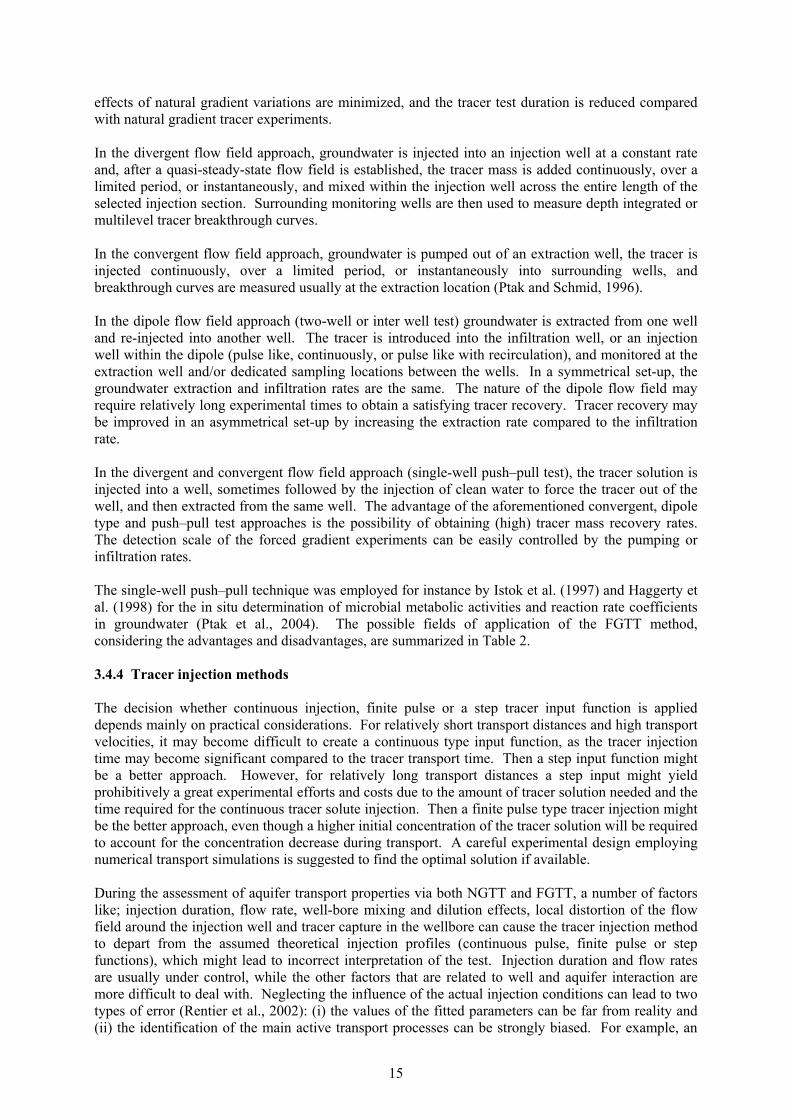
15
effects of natural gradient variations are minimized, and the tracer test duration is reduced compared with natural gradient tracer experiments. In the divergent flow field approach, groundwater is injected into an injection well at a constant rate and, after a quasi-steady-state flow field is established, the tracer mass is added continuously, over a limited period, or instantaneously, and mixed within the injection well across the entire length of the selected injection section. Surrounding monitoring wells are then used to measure depth integrated or multilevel tracer breakthrough curves. In the convergent flow field approach, groundwater is pumped out of an extraction well, the tracer is injected continuously, over a limited period, or instantaneously into surrounding wells, and breakthrough curves are measured usually at the extraction location (Ptak and Schmid, 1996). In the dipole flow field approach (two-well or inter well test) groundwater is extracted from one well and re-injected into another well. The tracer is introduced into the infiltration well, or an injection well within the dipole (pulse like, continuously, or pulse like with recirculation), and monitored at the extraction well and/or dedicated sampling locations between the wells. In a symmetrical set-up, the groundwater extraction and infiltration rates are the same. The nature of the dipole flow field may require relatively long experimental times to obtain a satisfying tracer recovery. Tracer recovery may be improved in an asymmetrical set-up by increasing the extraction rate compared to the infiltration rate. In the divergent and convergent flow field approach (single-well push–pull test), the tracer solution is injected into a well, sometimes followed by the injection of clean water to force the tracer out of the well, and then extracted from the same well. The advantage of the aforementioned convergent, dipole type and push–pull test approaches is the possibility of obtaining (high) tracer mass recovery rates. The detection scale of the forced gradient experiments can be easily controlled by the pumping or infiltration rates. The single-well push–pull technique was employed for instance by Istok et al. (1997) and Haggerty et al. (1998) for the in situ determination of microbial metabolic activities and reaction rate coefficients in groundwater (Ptak et al., 2004). The possible fields of application of the FGTT method, considering the advantages and disadvantages, are summarized in Table 2. 3.4.4 Tracer injection methods The decision whether continuous injection, finite pulse or a step tracer input function is applied depends mainly on practical considerations. For relatively short transport distances and high transport velocities, it may become difficult to create a continuous type input function, as the tracer injection time may become significant compared to the tracer transport time. Then a step input function might be a better approach. However, for relatively long transport distances a step input might yield prohibitively a great experimental efforts and costs due to the amount of tracer solution needed and the time required for the continuous tracer solute injection. Then a finite pulse type tracer injection might be the better approach, even though a higher initial concentration of the tracer solution will be required to account for the concentration decrease during transport. A careful experimental design employing numerical transport simulations is suggested to find the optimal solution if available. During the assessment of aquifer transport properties via both NGTT and FGTT, a number of factors like; injection duration, flow rate, well-bore mixing and dilution effects, local distortion of the flow field around the injection well and tracer capture in the wellbore can cause the tracer injection method to depart from the assumed theoretical injection profiles (continuous pulse, finite pulse or step functions), which might lead to incorrect interpretation of the test. Injection duration and flow rates are usually under control, while the other factors that are related to well and aquifer interaction are more difficult to deal with. Neglecting the influence of the actual injection conditions can lead to two types of error (Rentier et al., 2002): (i) the values of the fitted parameters can be far from reality and (ii) the identification of the main active transport processes can be strongly biased. For example, an

16
observed extended tailing and attenuation of the tracer breakthrough curve could erroneously be attributed to a kinetic sorption process or the occurrence of a dual porosity effect, when actually they are the result of the delayed release of the tracer, captured in the well at the end of the injection. 3.4.5 Multi tracer approach and DNA tracers As described above in the section dealing with the application of the gradient condition, see section 3.4.1, to reduce experimental efforts and to maximize gain of information from the generally costly tracer experiments, multiple tracers can be used within one experiment (Bosel et al., 2000). Then, groundwater samples have to be analyzed for multiple tracers. However, due to the physical and hydro-geochemical properties of the usually used fluorescent, gas or salt tracers, and the resulting limitations of the tracer analysis procedures, the maximum number of different tracer compounds that can be used in parallel would be limited. Another limitation with different tracers would require different analytical techniques such as fluorescence spectrometry, wet chemistry, ion chromatography and mass spectrometry that will require great experimental efforts. In the last few years, special tracing techniques involving synthetic DNA (deoxyribonucleic acid) molecules with individually coded information have been developed (Alestrom, 1995). With such new tracer compounds, it becomes principally possible to perform multitracer experiments with a theoretically unlimited number of tracers that could be injected at different locations with same analytical detection procedure. Theoretically, the detection limit goes down to one molecule (Watson et al., 1992). In addition to a practically unlimited number of different DNA sequences, meaning different tracers, the extremely low detection limit represents another huge advantage of using synthetic single stranded DNA molecules for tracing purposes in groundwater, compared to traditional tracers. The synthetic DNA molecules are usually available in 1 ml ampoules, which contain 1016–1018 identical molecules. Even if adsorbed, degraded and diluted under subsurface transport conditions by a factor of 1014–1015, which is much more than expected during standard hydro-geological applications, the tracers still remain easily detectable. One of the first experiments designed to test the mobility and migration of DNA coded molecules within sandy aquifers was performed at the Morrepen-3 research site, located near the Gardermoen Oslo airport in Norway (Sabir et al., 1999a and 1999b). 3.4.6 High resolution multi-level/multi-tracer sampling and concentration measuring equipment At some field sites with a high degree of heterogeneity, a three-dimensional subsurface characterization may become necessary, i.e. the measurement of depth-differentiated multilevel breakthrough curves. Multilevel sampling systems may be installed for this purpose (e.g. Ptak et al., 2000). However, especially at sites with deep aquifers and coarse aquifer material, monitoring well installation costs may become a limiting factor. To allow multilevel groundwater sampling also within fully screened pumping wells, avoiding installation of additional costly monitoring wells when performing forced gradient transport experiments, a flow separation technique was introduced (Ptak and Schmid, 1996). In this multilevel set-up, the screen within a pumping well is divided into individual measuring sections using a slotted-wall multilevel packer as shown in Figure 7. Each section can for instance be equipped with fibre optic probes for on-line in situ fluorescence spectrum measurements (for example if the transport velocity is relatively high, making round the clock frequent sampling necessary), and/or other probes yielding chemical and/or physical parameters. Mixing pumps can be provided in order to obtain parameter values representative of the entire section. Additional groundwater sampling tubes allow taking (level integrated) multilevel groundwater samples. In order to avoid vertical flow within the gravel pack during the multilevel sampling procedure, geo-textile clay seals can be installed within the gravel pack of the wells (Ptak and Kleiner, 1998). Geo-textile clay seals will make a separate room for each sampler.

17
3.4.7 Multi-tracer forced gradient transport experiments, investigation of physical and hydrogeochemical aquifer properties If the FGTT approach is used to investigate reactive transport processes, at least two tracers, a non-reactive and one or more reactive, are injected simultaneously at the same location into the aquifer. Since all tracers experience the same (heterogeneous) hydraulic conductivity field, the relative difference in the transport behaviour of the tracers (e.g. higher second order temporal moments of reactive tracer breakthrough curves compared to the non-reactive ones, relative retardation etc.) is only a statement of the reactive transport processes within the aquifer. Figure 8 shows the principle of this differential multi-tracer testing approach in a multi-level version. The multi-level version allows in addition the investigation of three-dimensional structural properties such as preferential flow paths, connectivity between investigated layers, structural anisotropy etc. The reactive tracer is chosen with respect to the reactive transport process investigated. Then, the parameter characterizing the reactive transport process can be deduced from the relative retardation of the reactive tracer with respect to the non-reactive tracer, if the relationship between the retardation factor and the process parameter(s) is known.
FIGURE 7: Multi level sampling within pumping wells (Ptak and Schmid, 1996)
FIGURE 8: Schematic sketch of forced gradient multi- level/multi-tracer approach (Ptak and Kleiner, 1998)

18
3.5 Tracer materials A variety of tracer compounds can be used. They can behave both non-reactive, i.e. as ideal tracers, and also reactive. The non-reactive, ideal tracers are used if the transport of solutes is being investigated; they are not subject to degradation or interaction with the subsurface material. Depending on the site specific subsurface conditions, ideal tracers might for example be salt based tracers such as Chloride (e.g. NaCl), Bromide (e.g. NaBr), fluorescent tracers such as Fluorescein, Eosine, Pyranine, Sodium–Naphthionate, Tinopal, radioactive tracers such as 1H3HO and 82Br, if the radioactive decay is accounted for, dissolved gas tracers such as He or H2, environmental isotopes and chemicals, or particle tracers such as natural, dyed, or fluorescent spores, fluorescent microspheres, other drift particles or DNA biological acids. Before selection of a conservative tracer compound laboratory testing should be performed to get the ideal or almost ideal tracer behaviour. In this section we will discuss the process of tracer material selection and we will cover two non-reactive tracer materials with their applications; Na-Fluorescein that has been used at the Hellisheidi-Threngsli injection site for the short tracer test, the subject of this research project, and SF6, which is to be used in the large scale test, both before CO2 injection and throughout the CO2 injection. 3.5.1 Tracer selection The tracer selected needs to meet a few criteria: (i) It should not be present in the reservoir or at a constant concentration much lower than the expected tracer concentration. (ii) It should not react with or absorb to the reservoir rocks. (iii) It should be easy (fast-inexpensive) to analyze. As described above in the section dealing with multi-level & multi-tracer tests, to reduce experimental efforts and to maximize the information gained from the generally costly tracer experiments, multiple tracers can be used within one experiment. Synthetic DNA materials or the same components with the mentioned ability will be the best group selection material for the ground water tracer test experiments. The synthetic DNA or synthetic carbon components (polymers) will likely be the next generation of the tracer test materials in the industry. The low detection limit up to a single molecule is another valuable advantage, which could help the small-scale tracer tests be observed precisely. Effort has to be made to define the behaviour of these tracer materials at different temperature, pH, geochemistry and host aquifer formation conditions. Now we can rewrite the criteria for tracer material as follows: a group of components with identical characters that could be detected with unique laboratory technique, which should not be present in the reservoir or at a constant concentration much lower than the expected tracer concentration and it should not react with or be absorbed to the reservoir rocks.
Radioactive materials are excellent tracers in natural environments and they are detectable at extremely low concentrations. They are, however, subject to stringent handling, transport and safety restrictions. The procedure for measuring radioactive tracer concentrations in samples collected is, furthermore, more complicated and time consuming than the procedure for measuring the concentration of most other kinds of tracers e.g. Fluorescein and Bromide. Aspects of environmental and administrative law have to be considered. In most countries, only a few compounds remain legal due to EIA mandates for injection in field experiments, mainly salt tracers and some fluorescent tracers. If new tracers, not yet known to the administration, are planned for injection, lengthy and tedious procedures to obtain permission for their use are required. 3.5.2 Na-fluorescein Sodium fluorescein (C20H10O5Na2), a highly water soluble fluorescent dye, is bright yellow-green to the eye and has a maximum excitation of 491 nm and maximum emission of 513 nm. Many groundwater-tracing studies have employed this dye since it is inexpensive, easily detectable, non-toxic, and stable over time (Gaspar, 1987; Smart and Laidlaw, 1977). It’s also detected at very low
19
levels of concentration (< 20 ppt). It can be measured using either its strong fluorescence or highly absorptive character (Klonis and Sawyer, 1996). Other advantages of fluorescein include its low sorption tendency (Behrens, 1986) and its relatively low temperature exponent (Feuerstein and Selleck, 1963). The disadvantages of fluorescein are its photochemical instability, pH sensitivity (Lindqvist, 1960). It has also been suggested that fluorescein solutions are unstable when heated (Leonhardt, et al., 1971). Therefore, sodium fluorescein has sometimes been regarded a non-quantitative tracer material. A number of studies that have examined the influence of pH, light, and heat on fluorescein, to demonstrate that fluorescein can be used for quantitative studies. In a series of experiments, which compare the degradation effects of pH, it has been shown that, it is possible to accurately predict the fluorescein absorptivity value at different pH values (Smith and Pretorius, 2002). In the same study fluorescein solutions exposed to sunlight show a rapid absorbance decrease. The average absorbance reduction for 2 hours exposure was 98% (solution without any additive component). This confirms that fluorescein degrades quickly in bright sunlight. Consequently in tests with fluorescein as a tracer the test area and samples must be protected from bright light. The simplest way to do this is to perform tests at night and to store samples in the dark. Studies have also shown that heated and room temperature fluorescein controls were stable throughout a 2 hour test period. The stability of these solutions compared with the instability of the sunlight exposed solutions showed that, it is more important to protect a fluorescein solution from bright light than from heat (Lindqvist, 1960). Fluorescein is easy to detect and relies on cost-effective and widely available analytical instruments. With reasonable precautions, fluorescein behaves conservatively. This suggests that fluorescein warrants re-evaluation as a quantitative tracer. Although the host aquifer is very important regarding the possible sorption of the tracer on the existing formation, there are a number of studies that observed the possibility of adsorption of fluorescein to clay compounds (Smart and Laidlaw, 1977). Sodium-fluorescein has been used successfully in numerous geothermal fields, both low-temperature ones and in higher temperature systems (Axelsson et al., 1995; Rose et al., 2000). 3.5.3 SF6 Sulphur hexafluoride, SF6, is considered a conservative tracer for experiments in groundwater and atmospheric applications. SF6 is an inert water-soluble gas, is biologically and chemically inert, has a low background concentration (10-15 mol/l), and can be detected at extremely low concentrations (Wanninkhof et al., 1985). Its estimated atmospheric lifetime is about 3200 years. SF6 can be routinely detected in ambient air and at extreme aqueous dilutions (i.e. ~ 10-17 mol/l) by electron capture gas chromatography (EC-GC). It is inert over a wide range of environmental conditions, non-toxic, inexpensive and safe to handle. Although it has an extremely high global warming potential, the effect as a greenhouse gas is still negligible because atmospheric concentrations are still rather low (Zoellmann et al, 2001). Sulphur hexafluoride, SF6, provides a technique for dating ground waters up to 50 years old. SF6 can help to resolve the extent to which groundwater mixing occurs, and therefore provide indications of the likely groundwater flow mechanisms. Atmospheric trace gases have been monitored at a number of sites across the globe for nearly 30 years (Prinn et al., 2000) and have been found to be generally well mixed, a factor underpinning their use in dating studies, see Figure 9 (e.g., Hohener et al., 2003).
The strong potential of SF6 as a geothermal tracer has also been reported (Wilson & Mackay, 1993). Important aspect of SF6 is its extremely low aqueous solubility, which gives it the potential to delineate unsaturated zones underground, an application to which non-volatile tracers are unsuited (Gooddy et al., 2006). With injecting SF6 to an aquifer and quantitative analysis, we can track the possible interlayer leakage or mixing of number of different groundwater systems in the area.

20
3.5.4 Tracer mass and sample collection frequency After a suitable tracer has been selected the mass of tracer to inject needs to be determined. Determination of necessary tracer mass, initial sample-collection time and subsequent sample collection frequency are the three most difficult aspects to estimate prior to a proposed tracer test. The mass needed can be calculated based on known field scale factors and measurements of discharge, transport distance, and suspected transport times. Basic field parameters commonly employed are often based on the original developers experience in a particular field. The following is a list of some important factors in mass calculation: Detection limit, tracer background (if any), injection rate (q) in the FGTT design, production rate (Q) in the FGTT design, number of wells involved and well locations, scale of the test (possible flow paths to estimate the dilution volume), return rate anticipated (slow/fast) based on available hydro-geological information or the scale of FGTT, density of water in the region or in the well (if density is different dye solution will sink and neither dilute nor transfer at the speed of the overall fluid in the aquifer). Moreover the tracer test strategy regarding the gradient condition will play a major role. The mass required may be estimated very roughly through mass-balance calculations, in which injection- and production rates are taken into account, as well as an expected recovery time-span. This time-span depends on the distances involved, but also on how directly the wells involved are connected. It is also practical to consider a measured concentration at least 5-10 times higher than the detection limit (DL) to be on the safe side. Numerous studies have been carried out to generalize equations for tracer-mass estimation and sample-collection frequency, see e.g. Field (2003). The empirically determined equations rely overall on two major methods; volumetric method and type curve method. In the volumetric method reservoir volume and dilution due to discharge rate in the block dictate the tracer mass amount. In this approach, two factors of time frame for test and length due to tortuosity will be added. For example if a test aims at short time recovery with FTTG strategy, less mass would be needed. In the type curve method, the adopted solution for the tracer study with the expected petrophysical parameter of the aquifer will be used to numerically predict the break through curve with various amounts of mass injection in the target block. An additional mass safety factor needs to be considered, which is simply aimed at protecting human health or the environment from excessive tracer –mass release. This mass is intended to ensure that adequate tracer mass is injected into the
FIGURE 9: Atmospheric concentration of SF6 in last 100 years used as calendar to mark the age of groundwater

21
system. In different studies and types of equations, this extra mass addressed in different ways but it is advised to obtain a final concentration 5 to 10 times the detection limit. The amount of tracer, or more precisely the tracer-excess coefficient, is dependent on type of tracer and host aquifer. For example as Kass (1998) indicated for Na-Fluorescein the excess factor is higher in clay aquifers than in fractured rocks or karst formation aquifers. Specific site related empirical equations have been developed as a by-product of many tracer test experiments in various host aquifers (Field, 2003). Whereas much effort has gone into methods of estimating tracer mass for tracing studies, very little appears to have been done in terms of determining sample-collection frequency. Sampling frequencies are generally based on travel distances, which are based on a direct relationship between travel distance and expected time of arrival. This relationship is obviously correct, but it’s ambiguous because transport velocity as a function of residence time is unknown. Transport velocities can achieve extreme ranges rendering invalid sampling schedules based on transport distances that are devoid of residence time estimates. But this can be overcome by recognizing that the average velocity is a rough estimate and represents a rough average travel time. The suggested sampling frequency can be appropriately adjusted to ensure that initial sample collection begins prior to likely tracer breakthrough (Ptak et al., 2004).

22
4. THE HELLISHEIDI–THRENGSLI SITE - NATURAL CO2 INJECTION LABORATORY The Hengill volcanic area, SW-Iceland, lies on the plate boundary between the North American and European crustal plates. These plates are diverging at a relative velocity of 2 cm/year. The rifting of the two plates has opened a series of north-northeast trending volcanic systems of normal faults and frequent magma intrusions in SW-Iceland. The Hengill volcanic and high-temperature geothermal area is a product of this tectonic and volcanic activity (Saemundsson and Fridleifsson, 2003). In tectonic terms the Hengill volcanic system lies at a triple junction, where the Reykjanes volcanic zone, the western volcanic zone and the South Iceland Seismic Zone meet. Mt. Hengill symbolizes the associated central volcano and rises about 550 m above its surroundings, to an elevation of 800 m a.s.l, (Figure 10). The natural formation of Mt. Hengill is a table mountain or Tuya. The main rock types in the Hengill area are interglacial lava flows and glacial hyaloclastite that are younger than 0.7 million years. Volcanic rocks of basaltic composition (of tholeiitic or olivine-tholeiitic type) cover a large part of the surface. The hyaloclastite ridges in the northeast, north, and west part of the area are composed of basaltic pillow lava, breccias and tuffs, which were formed during the last glacial period(s). Flat lying postglacial basaltic lavas cover the central parts of Hellisheidi, including postglacial lavas erupted 5000 and 2000 years ago (Saemundsson and Fridleifsson, 2003).
The Hellisheidi geothermal field is a part of the Hengill volcanic system. It is to the south of Mt. Hengill, and covers an area of about 40 km2, see Figure 10 (Saemundsson et al., 1990). The Threngsli field is at the southern part of the Hengill system and is located between two outcropping hyaloclastite formations, Lambafell to the west and Grahnukar in the east (Figure 11). The flat valley between them is covered with rough surfaced basaltic Aa lavas. The so-called CarbFix project will be carried out here, with the subsurface lavas being the target block for a CO2 injection study. Figure 10 shows an aerial photo of the Hellisheidi-Threngsli area and the location of Hellisheidi geothermal power plant (view from top of Mt. Hengill towards the south). The edge of the lava flows can be seen from the photo.
FIGURE 10: Map of Iceland with an aerial photo of the Hellisheidi-Threngsli area and the location of Hellisheidi geothermal power plant, view from top of Mt. Hengill toward south.
The neovolcanic zones and rift systems are shown on the map
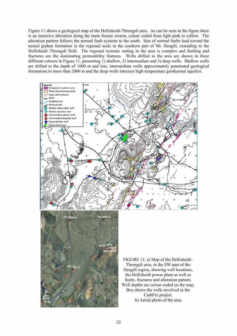
23
Figure 11 shows a geological map of the Hellisheidi-Threngsli area. As can be seen in the figure there is an intensive alteration along the main fissure swarm, colour coded from light pink to yellow. The alteration pattern follows the normal fault systems to the south. Sets of normal faults lead toward the nested graben formation in the regional scale in the southern part of Mt. Hengill, extending to the Hellisheidi–Threngsli field. The regional tectonic setting in the area is complex and faulting and fractures are the dominating permeability features. Wells drilled in the area are shown in three different colours in Figure 11, presenting 1) shallow, 2) intermediate and 3) deep wells. Shallow wells are drilled to the depth of 1000 m and less, intermediate wells approximately penetrated geological formations to more than 2000 m and the deep wells intersect high temperature geothermal aquifers.
FIGURE 11: a) Map of the Hellisheidi–
Threngsli area, in the SW-part of the Hengill region, showing well locations, the Hellisheidi power plant as well as faults, fractures and alteration pattern.
Well depths are colour coded on the map. Box shows the wells involved in the
CarbFix project. b) Aerial photo of the area b)
a)

24
The classification on the map in Figure 11 is based on depth, but it is also possible to classify them on different type of water. Shallow groundwater, which in part provides the drinking water supply in the area, with observed temperature of 0-6 °C located in the less than 100 m deep aquifers. Intermediate ground water flows in the most upper part of the geothermal fluid system and deeper than 400 m depth. Temperature below 100°C in the intermediate aquifer at 400 m to 1000 m depth, most likely results from earth thermal gradient and heat conduction. Temperature range is a good evidence of mixing of the intermediate ground water with the geothermal water in this section. The deepest system is believed to provide part of the high temperature geothermal fluid for the Hellisheidi system. Ground water dating and fluid chemistry were the major tools to distinguish the different type of fluids in the region although the stratigraphy gives some other clues to support this idea, see next section (Alfredsson et al., 2008). Wells HN-2, HN-4, HK-26 and HK-31 are drilled through the intermediate depth groundwater system, which along with wells HN-1, HK-12 and HK-25 are illustrated in right hand side of Figure 11. Except for wells HN-03 and HN-06, which are located further to the east, sited in the blue box, these are planned to be either an injection well or observation wells in the CarbFix project (Figure 11). These two wells were drilled deviated toward the main fissure swarm to intersect highly permeable faults nearby the active Mid-Atlantic Ridge shown in Figure 11. These faults define the western margin of the Hengill volcanic system. In the Hellisheidi development plan, these wells were planned for reinjection purpose as well as HN-02, HN-04 and HN-01. 4.1 The Hellisheidi–Threngsli CO2 injection site Figure 12 shows a simplified three-dimensional sketch of the region under consideration, including wells in the area (the area is marked by a blue box in Figure 11). Wells HN-02, HN-04, HK-26 and HK-31 are drilled through the intermediate depth groundwater system, while wells HN-01 and HK-25 only penetrate the shallow groundwater system above. Detailed stratigraphy of all wells in the area (Figure 13; Alfredsson et al., 2008), shows that from about 400 m depth, down to 800 m depth, aquifers are composed of fresh basaltic lavas interbedded with minor hyaloclastic layers/intrusions. This section has been referred to, as “the target zone” since the basaltic formation in this interval is the target zone for the CO2 injection experiment. Injecting CO2 at such depth will provide the possibility of water rock interactions that will fix the CO2 gas in carbonate minerals. Figure 13 shows the lithological cross section of the wells at the injection site. Based on lithological studies of drill cuttings three different lava flows have been distinguished in the region. The youngest lava flows at shallow depth in the Hellisheidi–Threngsli area are dated as 110-
FIGURE 12: Simplified three-dimensional sketch of the Hellisheidi–Threngsli CO2 injection target zone, showing the injection and monitoring wells in the block

25
125 thousand years old. The second set which dates back to 300 thousand years ago, is at approximately 400-800 m a.s.l. depth. The third set, the oldest one, has been traced in some wells to depth greater than 1000 m. Each sequence of lava flows has a fine to medium size grain texture, though coarse grain sizes were also found (very rare) in the sections studied (Alfredsson et al., 2008). Between lava flows interbedded layers of tuff, basaltic breccias and hyaloclastites could be seen. The detailed stratigraphy of wells HN-02 and HN-04 is illustrated in Figure 16 and Figure 18.
Tracer testing is being used as an advanced tool to investigate the petrophysical characteristic of the target zone. A series of tracer tests is being planned during the CarbFix project life-time; initially for aquifer characterization of the target zone and later for precise monitoring of the possible changes after CO2 injection. To obtain information on the parameters needed to delineate the CO2 injection strategy an initial short tracer test was conducted between wells HN-04 and HN-02. The purpose of the test is to try to add to the understanding of the nature of the groundwater system, including flow-patterns and flow-rates as well as the contribution of different aquifers, intersected by the wells, to the flow transport process. 4.2 Porosity and permeability structure in the Hellisheidi-Threngsli area A general phenomenon in both surface hydrology and geothermal reservoir studies is the dual porosity nature of Icelandic rocks and the bipolar distribution of permeabilities. Experience shows that most of the fluid circulating in geothermal reservoirs flows through a few widely spaced (tens, hundreds of meters) tectonic fractures. The flow through the intervening rock sequences, which probably occurs through a connected network of pores and micro-cracks, is in most cases insignificant by comparison (Hardarson et al., 2007). Information on the porosity and permeability at the Hellisheidi-Threngsli is directly and indirectly based on two set of data that have been studied at two different scales. First regional information from sections studied in the target area that have been drilled and exposed to pumping tests. These large-scale studies were directed more toward tectonic fractures and their significant contribution to fluid
FIGURE 13: NE-SW cross section through the Hellisheidi-Threngsli field, showing the three main lava flow sections and interbedded hyaloclastites (Alfredsson et al., 2008)
26
extraction in the aquifers. Second, a number of studies aimed at finding an empirical relationship between permeability and porosity in the laboratory scale using the olivine tholeiite lava sequences, which are common reservoir rocks in Icelandic geothermal systems, the same as our target aquifer. Fracture porosity and fracture permeability are difficult to study in the laboratory because fractures are frequently underrepresented in the samples. Fractured samples often fall apart and are discarded. The study of laboratory size samples are on the other hand directed more towards the rock matrix permeabilities of aquifer systems. The drilling of several wells, in particular in the western part of the Hellisheidi area, has provided valuable information (Alfredsson et al., 2008). Lithological data of wells HN-01, HN-02 and HN-04 have shown that they vertically penetrated lava flow sequences and hyaloclastite bodies and they did not intersect any faults or fracture settings in the area (Hardarson et al., 2007). Well measurement data during the injection and production test of these wells also indicated that they did not have good permeability, however, the directional wells, HN-06 and HN-03, which have an inclination toward the fissure swarms and intersect major faults and fractures, provide good permeability and high injectivity indices, (Figure 11). Based on these observations, we can say that the main permeability in the area is due to fractures and faults (Hardarson et al., 2007). The lava flow sequences and interbedded layers are not good aquifers in terms of fluid delivery. Even observed disconformities due to different lava flows, or a lava flow layer over a layer of hyaloclastite in wells HN-02 and HN-04 did not provide a comparable permeability with the fracture permeability in wells HN-06 and HN-03. A number of studies have evaluated the petrophysical behaviour of the lava flows aimed at finding an empirical relationships between permeability and porosity (e.g. Franzson et al., 2005; Frolova et al., 2005). Gudlaugsson (2000) presents the results of a microscopic scale study of porosity and permeability characteristic of lava flows in Öskjuhlíd in Reykjavík. In this research study, a large number of core samples were taken from the Öskjuhlíd lava flow. The approach chosen was to make a large number of measurements of thermal conductivity parameters in a homogenous rock spanning a wide range of porosities. The Öskjuhlíd lava flow was selected for the study, because olivine tholeiite shield lavas were thought to meet these criteria, and about 100 samples were obtained for analysis. As olivine tholeiite lava sequences is the main host rock of the target zone, this study is considered quite relevant to our research. In order to make sure that the lava flow was homogenous, the mineralogy was studied in thin sections and the chemical composition analysed. In addition to thermal conductivity and porosity, measurements were also made of the permeability, sonic P-wave velocity and grain density and also to check that the Öskjuhlíd samples were petrophysically well-behaved, i.e. did not show any unusual petrophysical behaviour that might affect the study of the thermal conductivity-porosity relationship (Fridleifsson et al., 1997). During analysis of the data, however, unusual interrelationships between the petrophysical parameters emerged. In short, it was discovered that permeabilities in the core of the lava flow, where the porosity is at a minimum, were more than an order of magnitude higher than at the vesicular top and bottom of the flow. This behaviour is opposite to the general trend of an empirical relationship between permeability and porosity in Icelandic rocks presented by Sigurdsson (2000). With use of conventional methods (microscopic and thin section analysis) two main types of pores, based on geometry, were found in the Öskjuhlíd lava flow core samples. A vesicular type pore space, characterized by smooth, round, glass-rimmed vesicles with fine to middle grained matrix that dominates the margins of the flows. By contrast, irregular inter-crystalline pores, set between the grains of a coarse-grained matrix, characterize the inner parts of the flows (Fridleifsson and Vilmundardottir, 1998). The transition between the two states is fairly sharp, but occurs at somewhat higher porosities than the transition between high and low permeabilities. Another feature also observed was the presence of abundant microcracks at grain boundaries within the sampled rock matrix (Johnson et al., 1998).

27
The preferred explanation of the permeability anomaly is that the presence of an extensive, connected network of grain-boundary microcracks is the feature that causes higher permeability in the coarse-grained inner part of the flow. Changes in the ratio of vesicular to inter-crystalline porosity and the influence of a low-permeability glass coating around vesicles are unlikely to be the primary causes of the anomaly. The microcracks are probably created by seismic activity. Testing of this hypothesis is possible by further measurements, but based on this study too few samples have been tested to provide conclusive results. There is especially a need to evaluate this hypothesis at high pressure conditions to extrapolate the result for deeper part of the reservoir, although it is probably the case in shallow and intermediate depth layers (Gudlaugsson, 2000). According to this hypothesis the reason for relatively high permeability of the lower porosity region, i.e. the inner structure of the lava flows in a seismically active region like the Hellisheidi-Threngsli area, is a network of interconnected porosities. We can propose that the total available porosity in a network of microcracks that interconnect all medium size pore spaces together, will create higher permeability relatively to the more porous margins. Furthermore, the flow-path tortuosity will be quite high in such a permeable layer. It should be emphasized, however, that this is possible because of the limited alteration of the basalt involved. And also that interbeds between layers may in some cases be more permeable than the internal parts of lava-flows. 4.3 Target wells Wells HN-04 and HN-02 are located in the northern part of the target block, see Figure 11 and Figure 12. The wells are located in the western flank of the Lambafell hyaloclastite outcrop and at the entrance to Threngsli valley quite close to the road. They are drilled from the same platform and the distance between the wells at the surface is 9 m and 60 m at 400 m depth. The plan is to use HN-02 as the injection well for the CO2 experiment. To evaluate the petrophysical characteristics of the aquifers in-situ, HN-02 was selected as a base well for the execution of tracer tests experiments. During the initial short tracer test well HN-2 was used as a tracer injection well and well HN-04 as the main observation well. Wells HN-01, HK-31 and HK-26 were also monitored but less frequently than HN-04. Wells HK-31 and HK-26 are located about 1500 and 2700 m down-stream, while HN-01 was the water supply well for the tracer test, see Figure 11 and Figure 12. Here we will discuss in more details the data available from the two main wells (HN-02 and HN-04) through different well studies. 4.3.1 Well HN-02 Well HN-02 is a deep vertical well located in Threngsli. Its coordinates are: X = 381140.2 m, Y = 393771.3 m and Z = 265.5 m a.s.l. with a total true vertical depth of 2001 m. The original purpose of the well was to find the best well site for the reinjection strategy of the 90 MWe unit of the Hellisheidi power plant (commissioned in 2006). Its location was selected downstream from the Hellisheidi well field for the disposal of waste geothermal fluid from Hellisheidi steam wells. A number of temperature logs were measured for this well during drilling and afterwards (Figure 14). The logs were measured during shut-in, injection and production conditions. In the target zone (400 – 800 FIGURE 14: Temperature profiles
for well HN-02

28
m depth) the temperature is less than 100°C, while the contribution of high temperature aquifers can be observed in the deeper parts of the well. Six depth-intervals have been proposed as possible aquifers, or feed-zones, located in the uppermost part of the well (Figure 14). Based on the temperature difference of injected mud and exit mud after circulation (Figure 15), we can see the well does not show a major aquifer before stimulation and overall, the well is relatively tight with very low contributions of aquifers. The amount of drilling fluid loss during drilling hardly indicate major permeable aquifers in the target zone and the temperature profile of the drilling fluid follows a constant thermal gradient. Figure 16 shows a detailed geological column for the well, based on analysis of drill cuttings (Franzson et al., 2004). It also shows the location of possible aquifers in the first 1000 m of the well. The major aquifer located at 400 m depth coincides with a sudden change in lithology as well as being observed in the temperature logs (Figure 16). A medium grain basaltic lava section starts at 400 m depth and continues down to 800 m depth. Basaltic lava flows comprise most of the thickness of the target zone down to the
FIGURE 15: Temperature changes of drilling fluid before injection and after circulation during drilling of well HN-02. Temperature jumps
show possible aquifers or feed-zone locations
Small aquifer
Medium aquifer
Major aquifer
Intermediate-fine grained rock
Intermediate-coarse grained rock
Medium-coarsed grained basalt
Coarse grained basalt
Intermediate Tuff
Scoria
Basaltic Tuff
Basalatic brecia
Poorly crystalized basalt
Fine-medium grained basalt
Intermediate brecia
FIGURE 16: Lithological log and possible aquifer locations in well HN-02 for the first 1000 m depth, where the total true vertical depth is 2001 m (Franzson, 2004)
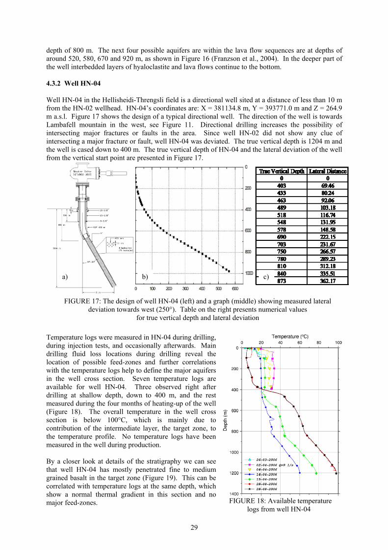
29
depth of 800 m. The next four possible aquifers are within the lava flow sequences are at depths of around 520, 580, 670 and 920 m, as shown in Figure 16 (Franzson et al., 2004). In the deeper part of the well interbedded layers of hyaloclastite and lava flows continue to the bottom. 4.3.2 Well HN-04 Well HN-04 in the Hellisheidi-Threngsli field is a directional well sited at a distance of less than 10 m from the HN-02 wellhead. HN-04’s coordinates are: X = 381134.8 m, Y = 393771.0 m and Z = 264.9 m a.s.l. Figure 17 shows the design of a typical directional well. The direction of the well is towards Lambafell mountain in the west, see Figure 11. Directional drilling increases the possibility of intersecting major fractures or faults in the area. Since well HN-02 did not show any clue of intersecting a major fracture or fault, well HN-04 was deviated. The true vertical depth is 1204 m and the well is cased down to 400 m. The true vertical depth of HN-04 and the lateral deviation of the well from the vertical start point are presented in Figure 17.
Temperature logs were measured in HN-04 during drilling, during injection tests, and occasionally afterwards. Main drilling fluid loss locations during drilling reveal the location of possible feed-zones and further correlations with the temperature logs help to define the major aquifers in the well cross section. Seven temperature logs are available for well HN-04. Three observed right after drilling at shallow depth, down to 400 m, and the rest measured during the four months of heating-up of the well (Figure 18). The overall temperature in the well cross section is below 100°C, which is mainly due to contribution of the intermediate layer, the target zone, to the temperature profile. No temperature logs have been measured in the well during production. By a closer look at details of the stratigraphy we can see that well HN-04 has mostly penetrated fine to medium grained basalt in the target zone (Figure 19). This can be correlated with temperature logs at the same depth, which show a normal thermal gradient in this section and no major feed-zones.
FIGURE 17: The design of well HN-04 (left) and a graph (middle) showing measured lateral deviation towards west (250°). Table on the right presents numerical values
for true vertical depth and lateral deviation
a) b) c)
FIGURE 18: Available temperature logs from well HN-04

30
Five possible aquifers are seen in the well (Figure 19) of which the shallow ones are believed to be the major ones based on evidence revealed by borehole geology during drill cutting studies (Franzson et al., 2004). The first three aquifers are located above 100 m depth, i.e. behind the 400 m casing. In the target zone, the only major aquifer is located at about 400 m true vertical depth and it also seems responsible for the temperature rise in the temperature profiles around the same depth. No major indications of possible aquifers are observed in the deeper part of the well except for a minor aquifer at 830 m depth. The effect of a deep aquifer can also be seen in the temperature profiles, see Figure 18. 4.4 Governing flow direction and velocity in the intermediate ground water system Based on a number of observations in different wells in the area it is believed that the drainage in the Hellisheidi-Threngsli field is towards south. This is based on noble gas dating and SF6 concentrations in the aquifers. Water level measurements in existing wells, over a period of two years, have shown that the water level drops towards the south. Surface elevation also declines towards the coast, which supports the idea of the flow direction being to south, towards the coast. Three water level data points were used to evaluate the possible velocity in the intermediate aquifer. Table 3 shows the selected wells and water level measurements. These are well HN-01 located in the northern part of the field, HK-31 in the middle and HN-26 is located in the southern part. The distance from HN-01 to HK-31 is 1.2 km and 1.8 km to HK-26, see Figure 11. The velocity is estimated for a cross section through wells HN-01, HN-31 and HK-26. With two basic assumptions, these numbers were used to estimate the possible velocity range in the intermediate ground water system in the area. First the value for the
FIGURE 19: Lithological log and location of possible aquifers in well HN-04 (Franzson et al., 2004)
Intermediate-fine grained rock
Intermediate-coarse grained rock
Medium-coarse grained basalt
Coarse grained basalt
Intermediate Tuff
Scoria
Basaltic tuff
Basalatic breccia
Poorly crystalized basalt
Fine-medium grained basalt
Intermediate brechia
Small aquifer
Medium aquifer
Major aquifer

31
overall permeability was chosen as the value estimated on basis of the longest pumping test which has been performed in the area (2007-2008), 400 mDarcy (Aradottir, personal communication). The second assumption is that the time difference between measurements is negligible as well as the effect of any other interference, like from other pumping test or other dynamic conditions in the block. The assumed value for the permeability is believed to be an underestimate based on parallel numerical calculation by other partners in the project.
TABLE 3: Water level measurements and elevation of wells HN-01, HK-31 and HK-26
By using Equation 4 and the data in Table 3, the seepage velocity is estimated to be of the order of 7.2 x10⁻⁷ (m/s). Assuming an effective porosity of 0.25 and groundwater with temperature of 25°C, the seepage velocity, or linear velocity, is estimated to be about 23 m per year using Equation 6. According to this value, it will take ~132 years for water to travel from the northern part of the field to the southern part (HN-01 up to HN-26) through the specific layers of the target zone. Keep in mind that the value is a rough estimation of fluid travelling through a homogeneous layer with an average permeability of 400 m D and neglecting any fractures or faults. 4.5 Execution of the initial short tracer test Exactly 500 g of Na-Fluorescein tracer were diluted with 100 l of water. The solution was flushed as a slug into well HN-02. The amount was based on simple mass balance estimates. Results of laboratory experiments simulating reservoir conditions carried out concurrent with a reinjection project at Laugaland in N-Iceland to study the thermal stability and sorption tendency of Na-fluorescein (Hauksdottir et al., 2000) were also taken into account. Na-Fluorescein has shown conservative behaviour for basaltic host formations and the temperature condition of the reservoir (Axelsson et al, 2001). The results of these experiments indicate that Na-fluorescein neither decays at the reservoir temperature in question (95-100°C), nor interacts with the low-altered minerals in the basaltic rocks of the reservoir, over the relevant time-scale (several months). As has been observed the temperature range of our experiment, i.e. in the target zone, is below 100°C and the alteration is minimal in the well cross sections (Hardarson et al., 2007; see Figure 11). Therefore Na-Fluorescein can be regarded as a conservative tracer regarding thermal decay or sorption. During planning of the test two methods were applied to estimate the amount of tracer needed. Assuming even dilution in the target rock volume and by using modelling by a theoretical breakthrough curve based on the dispersion model adopted, see section 4.6. Such forward modeling was also applied when setting up a sampling frequency plan (Axelsson, 2007). The tracer slug was injected into well HN-02 at 10:10 on 12.11.07. The test was continued up to early May 2008. The test was carried out under forced gradient conditions induced by a continuous doublet operation by injecting 5.5 kg/s of water into well HN-02 and pumping of 10.5 kg/s of water from HN-04. Pumping was initiated three days prior to tracer injection so that semi steady-state conditions would be in effect in the aquifers. The water was supplied by well HN-01 located about one km from HN-02 to the west, see Figure (11). The short distance, between the wellhead positions of HN-02 and HN-04, increases with the depth of the wells. Right after the kick-off point in well HN-04 at 200 m depth the offset between the wells increases as shown in Figure 17. Of the wells drilled through the basaltic target aquifer, these two wells are those closest to each other. The short distance is expected to result in a much higher rate of recovery compared to the large scale
Measurment date Well Measured water level (m)
Well elevation a.s.l. (m) Water level
5.4.2005 HN-1 110 286.5 176.526.9.2007 HK-31 103.33 274.4 171.07
18.10.2006 HK-26 89.37 256.4 167.03

32
tracer test planned between wells located far apart. Figure 20 shows the surface set-up for the short test and location of the wells. Each flow tube was equipped with a flow meter to record the flow rate and the wells were also equipped with pressure gauges recording the pressure changes in the wells throughout the test. 4.6 Theoretical solution adapted for the Hellisheidi-Threngsli short tracer test In order to define the amount of tracer material needed, to set up an appropriate sampling plan and to simulate tracer breakthrough concentration, a one-dimensional dispersion transport process was assumed. Such a model ignores diffusion and adsorption. The induced velocity due to the dipole test was assumed to result in one-dimensional flow from injection well to pumping well. As the assessment based on available data showed that the natural governing flow velocity in the block is much lower than the forced velocity in the aquifer in dipole test, therefore lateral vector of groundwater velocity was neglected. Based on the theory of solute transport Equation 23 the governing equation of the tracer movement in a one- dimensional dispersion transport is as below:
tC
xCu
xCD xh ∂
∂+
∂∂
=∂∂
2
2
(28)
Where Dh is the dispersion coefficient (m2/s), called the coefficient of hydrodynamic dispersion in groundwater, C is the tracer concentration in the flow-channel (kg/m3) and ux the fluid velocity in the channel (m/s). Effective molecular diffusion is neglected in this simple model such that
∗+= mLh DDD , xLLhm uDD~D ⋅==→∗ α0 with Lα the longitudinal dispersivity of the channel (m), see discussion in section 2.6. Assuming instantaneous injection of a mass M (kg) of tracer at time t = 0, and considering that the tracer mass will just pass through the void volume of rock, Aφ , the solution will be as below:
(29)
The flow between injection and production wells may be approximated by one-dimensional flow in flow-channels. These flow-channels may, in fact, be parts of near-vertical fracture-zones or parts of horizontal interbeds or layers. These channels may be envisioned as being delineated by the boundaries of these structures, on one hand, and flow field stream-lines, on the other hand. In other cases, these channels may be larger volumes involved in the flow between wells. In some cases more than one channel may be assumed to connect an injection and a production well, for example connecting different feed-zones in the wells involved. Based on above description the flow paths are simplified to a number of channels between wells (Axelsson et al., 2005).
FIGURE 20: Surface set-up for the short tracer test between wells HN-02 (injection) and HN-04 (production) in the Hellisheidi–Threngsli field
tDutx
h
LetDA
MtC 4/)( 2
21)( −−=πϕ

33
Based on conservation of the tracer we can write C·q= c·Q, where C is concentration of tracer in the flow channel as it enters the production well and q is the flow rate (kg/s) in the flow channel, which delivers the flow to the production well, as it connects with the production well. In addition Q is the production rate (kg/s) and c the tracer concentration in the production well fluid, i.e. at the observation point. We define the average fluid velocity in a flow channel by u,= q/ρAφ (m/s), with ρ the water density (kg/m3), A the average cross-sectional area of the flow-cannel/channels (m2) and φ the flow-channel porosity. Rewriting Equation 29 with this assumption it becomes:
DttuxeDtQ
Mutc 4/)(,
2,
21)( −−=π
ρ (30)
The above equation was used for the tracer test analysis presented later in this report. Such a simulation yields information on the flow channel cross sectional area, actually Aφ, the longitudinal dispersivity αL, as well as the mass of tracer recovered through the channel. This mass should of course be equal to, or less than, the mass of tracer injected. In the case of two or more flow channels, the analysis yields estimates of these parameters for each channel. It should be pointed out that through the estimate for Aφ the flow channel pore space volume, Aφx, has in fact been estimated. The tracer interpretation software TRINV was used for the simulation and interpretation (United Nations University Geothermal Training Programme, 1994). TRINV uses an automatic non-linear least-squares inversion technique to simulate the data and to obtain the model properties, i.e. the flow channel volume Aφx and dispersivity αL. This method has been used successfully in early stage interpretation in a number of geothermal fields worldwide (Axelsson et al., 2005). 4.6.1 Required mass of tracer To estimate the required mass of tracer a method of even dilution in the entire volume, and a method of simulation were used, as already mentioned. For an even dilution scenario a cubic volume of rock was considered based on the test set-up. Convergent FGTT test set-up was planned with a production rate twice the injection rate. In such a set-up the resulting flow paths can be expected to be more closely spaced than for radial flow. Also, applying a tracer test over a short distance will result in lower dispersion and consequently the mass of tracer required will be less. Local heterogeneity cannot interfere much with the flow paths to increase the mechanical dispersion on a macro scale, such that we can assume that they penetrate more or less the same aquifers (Figure 16 and Figure 18). A 100 m wide, 100 m long and 100 m high reservoir was considered, with a porosity value of 0.25. With half a kg of Na-Fluorescein diluted evenly in this volume, the concentration will be of the order of ~2 ppm throughout the volume. The detection limit for Na- Fluorescein is 10-20 ppt, which will provide an excess margin three orders of magnitude over the detection limit. Based on the theoretical solution adopted i.e. Equation 30, a calculation has been performed for 0.5 kg tracer mass and different distances between wells. Figure 21 illustrates the results based on assumptions listed in the table attached. The results in Figure 21 show that to detect a breakthrough of 0.5 kg of tracer 60-200 m down-stream requires resolution of about 0.02 – 0.005 ppm. This is some order of magnitudes lower than the concentration estimated on basis of an even dilution in the reservoir volume. This is still significantly higher than the detection limit of Na-Fluorescein. 4.6.2 Sample collection frequency As Figure 21 predicts based on the assumptions made, a fast breakthrough was expected and the sampling from well HN-04 was carried out at a rate of 4 samples per day for the first two weeks. Early sampling at a high frequency will enable the detection of fast breakthroughs, although the plan could be revised throughout the test as more data become available. The tracer test sampling plan was revised in our experiment as the observed concentrations showed a much slower transport than had been anticipated. After the first two weeks, sampling frequency was reduced to one sample per day

34
for 125 days and one sample per week during the last 3 weeks of the test. Samples were also collected from wells HN-01 and HK-31 to detect any possible lateral flow and tracer sweep toward the other wells, see Figure 11 and Figure 12 for their locations. Well HN-01 supplied the water for the injection well HN-02 and HK-31 is located 1.5 km downstream, to the south. No tracer was detected in these two wells during the test. We should also keep in mind that before tracer test execution the wells involved were sampled to detect the background level of the tracer for possible residual tracers in the fluid from former tracer tests. The results did not show any concentration of Na-Fluorescein in these wells. Baseline measurements are prerequisite for any geochemical analysis experiment in groundwater. 4.6.3 Sample analysis and breakthrough curve Great care was taken in the sampling process, by using dark sampling bottles and by keeping samples in cold and dark places to avoid any possible decay effect during storage. Figure 22 shows one of the sampling bottles. In addition care was taken to avoid having the personnel involved in the tracer injection near the sampling wells, at least initially. The Na-Fluorescein concentrations in the samples were determined with a Turner Designs TD-700 Fluorimeter, which provides exact concentrations after calibration. The fluorimeter mainly used a 10-089 blue mercury vapour lamp, 10-105 excitation filter (486 nm), and a 10-109R-C emission filter (510–700 nm), as specified by the manufacturer, see Figure 23. The tracer recovery data for well HN-4 during the initial short tracer test are shown in Figure 24. The filled squares in Figure 24 show the measured tracer concentrations. Overall two humps can be seen in the recovery curve. Some data points are off from the general trend. This may result from uncertainties regarding sample handling or light exposure. In later simulations these data points have been filtered out. The total mass recovery in the tracer test was 42%. Considering a FGTT execution the recovery factor is generally assumed to be much higher than this (Kass, 1998). According to the prediction of the breakthrough curve in Figure 21, a much faster recovery was also expected. At the 200 m distance the recovery was expected to be 50% after 20 days and in the case of shorter flow paths 50% after half a month.
FIGURE 22: Sampling bottle for Na-Fluorescein sampling and sanitary gloves
FIGURE 21: Theoretical tracer recovery curves for a 100 m wide and 100 m thick groundwater
reservoir with 25% porosity, dispersivity (αL) of the order of 100 m and one-dimensional flow.
Half a kg of an arbitrary tracer is injected at time t = 0. Recovery curves for distances
60, 100 and 200 m are shown
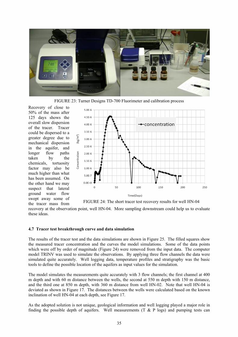
35
Recovery of close to 50% of the mass after 125 days shows the overall slow dispersion of the tracer. Tracer could be dispersed to a greater degree due to mechanical dispersion in the aquifer, and longer flow paths taken by the chemicals, tortuosity factor may also be much higher than what has been assumed. On the other hand we may suspect that lateral ground water flow swept away some of the tracer mass from recovery at the observation point, well HN-04. More sampling downstream could help us to evaluate these ideas. 4.7 Tracer test breakthrough curve and data simulation The results of the tracer test and the data simulations are shown in Figure 25. The filled squares show the measured tracer concentration and the curves the model simulations. Some of the data points which were off by order of magnitude (Figure 24) were removed from the input data. The computer model TRINV was used to simulate the observations. By applying three flow channels the data were simulated quite accurately. Well logging data, temperature profiles and stratigraphy was the basic tools to define the possible location of the aquifers as input values for the simulation. The model simulates the measurements quite accurately with 3 flow channels; the first channel at 400 m depth and with 60 m distance between the wells, the second at 550 m depth with 150 m distance, and the third one at 850 m depth, with 360 m distance from well HN-02. Note that well HN-04 is deviated as shown in Figure 17. The distances between the wells were calculated based on the known inclination of well HN-04 at each depth, see Figure 17. As the adopted solution is not unique, geological information and well logging played a major role in finding the possible depth of aquifers. Well measurements (T & P logs) and pumping tests can
FIGURE 23: Turner Designs TD-700 Fluorimeter and calibration process
FIGURE 24: The short tracer test recovery results for well HN-04

36
provide the first estimate of the number of flow channels prior to simulation. Reviewing the locations of possible aquifers based on stratigraphy, well logging and drilling fluid temperature change lead us to 3 depths. The 400 m depth has been confirmed by high temperature difference in injected and pumped drilling fluid in well HN-02 (Figure 15) and in the lithological log a sudden change in the stratigraphy from basaltic tuff to fine - medium grained basalt in HN-02 and HN-04, which borehole geologist has marked as a possible feedzone in the sections (Figure 16 and Figure 18). The second feed zone is believed to be at 550 m depth, while from 400 m depth to 1500 m depth well HN-02 did not show a sudden temperature jump neither in temperature logs nor in drilling fluid, and it follows a normal thermal gradient (Figure 14 and Figure 15). But, there are indications like a calcite vein from 520 to 570, which is considered by borehole geologists as a possible aquifer (Figure 16). This section is the same in both wells although the calcite veins were more dominant in HN-02 than in HN-04. The section consists of fine-medium grained basalt in both wells (Figure 16 and Figure 18). A second channel was defined to represent the contribution of this section to the tracer breakthrough curve. There was a slight difference in trend of temperature logs seen at 800m true vertical depth of HN-04 according to a temperature profile measured on 14.04.2006 (Figure 19) and to borehole geology (Franzson, 2004). This marks a minor aquifer at 820 m depth (Figure 18). In HN-02 at 800 m depth the stratigraphy changed from basaltic tuff to medium grained basalt, although notes regarding the minor or major aquifers were not indicated by borehole geology (Figure 16). This depth is considered as representing the deepest flow channel involved in the tracer test. The individual dashed-curves in Figure 25 represent the concentration contribution of each channel assumed, and the solid curve represents the sum of the three calculated concentrations. The sum of the three channels fits the measured concentrations quite nicely (coefficient of determination is 96.8%). Mass balance can be used to calculate the mass recovery of the tracer through individual channels. The total theoretical mass recovery of the tracer test was 50%. The parameters of the three assumed channels are shown in Table 4. These are flow path distance (x), assumed flow-channel (aquifer) depth, the calculated mass recovery of tracer through the corresponding flow channel, until infinite time, over the total injected tracer (Mi/M), dispersion coefficient (DL), fluid velocity (ux), the simulated product of flow channel area A and porosity φ, and longitudinal dispersivity (αL). TABLE 4: Model parameters used to simulate the tracer recovery with 3 channels; flow path distance (x), the calculated mass recovery of tracer through the corresponding flow channel, until infinite time
over the total injected tracer (Mi/M), dispersion coefficient (DL), fluid velocity (ux), the simulated product of flow channel area A and porosity φ (m2) and longitudinal dispersivity (αL)
Channel X (m) Depth (m) Mi/M DL(m2/s) u (m/s) Aφ (m2 ) α L
1 60 400 3.2 5.20E-03 8.20E-05 2.3 63.32 150 650 34.5 7.40E-04 4.50E-05 47 16.53 360 850 12.3 1.00E-01 5.20E-05 14 20.4
FIGURE 25: Observed and simulated Na-fluorescein recovery in well HN-04 assuming three distinct flow channels

37
4.8 Simulation result discussion The first hump in Figure 25 shows the contribution of a small volume aquifer to the total observed concentration, which may correspond to a thin interlayer or a fracture between the wells at shallow depth. Lithological stratigraphy shows a sharp change at 400 m depth in both wells, from hyaloclastite to lava flows. This unconformity may cause this fast tracer arrival. The calculated mass recovery of tracer through this flow channel was small, or 3.2 % (Table 4). The second pulse in Figure 25 is most likely caused by a much larger aquifer in the well cross section. Turning back to the feed-zone locations in well HN-02, likely tracer transport aquifers are sited at 500, 650 and 750 m depth, which all could be interpreted as inner parts of lava flows with higher permeability, below the main aquifer at 400 m depth. Possible aquifers have not been distinguished below 400 m depth in well HN-04, especially in the part of the well from 500 to 800 m depth. But based on lithology 650 m depth is considered as a representative depth for the set of lava flows seen in well HN-02. It is believed that their contribution is that of a thicker layer with semi uniform transport process delivering most of the tracer. The calculated mass recovery of tracer through this flow channel was 34.5% of the total injected tracer (Table 4). The classic shape of the curve characterizes a homogeneous porous medium in the channel. The unusual permeability behaviour of the olivine tholeiite lava of the Öskjuhlíd formation referred to in chapter 4.2 of this report may also be the case in this layer. The contribution of the interlayer transport is important because of higher permeability and the smaller matrix grain size and high tortuosity will make a longer flow path and recovery slower than what has been anticipated. Although the hypotheses of the less porous interlayer with higher permeability has not been proven in high pressure experiments, a network of micro cracks is most likely in the highly active region of the Hellisheidi-Threngsli area. This network cannot deliver a large amount of fluid but will cause dispersion and high reactive surface area for the fluid that passes through it. Channel 3 is assumed to represent the effect of an aquifer at approximately 850 m depth, which was well defined in the last section of the wells (see section 4.3.1 and 4.3.2). This aquifer responded much later as a consequence of its depth and greater distance between wells (Figure 25). The mass recovery contribution calculated for this aquifer is 12.3% (Table 4). Despite of extended recovery time about 50% of the tracer mass has not been recovered. This may indicate that either a longer recovery period would have been needed or that natural lateral flow in the ground water system has washed half the tracer away. The calculated velocity of ground water based on water level is not considered high enough to have such effect. Therefore, it is likely that the flow velocities are considerably higher in parts of the target interval. Weather a late arrival of the tracer due to tortuosity along the flow path or diffusion to dead points trapped the tracers, can’t be ruled out, however. The highest transport velocity was simulated for channel one (Table 4), bearing the sign of fracture behaviour. The velocity was less in channel 2, which along with a higher concentration of the second pulse suggests a thicker layer. The third channel showed a higher velocity than channel number 2 but its contribution arrived toward the end of the total concentration curve due to its greater length and deeper location in the well (Table 4 and Figure 25). Channel 1 had the smallest pore volume, as expected for a fracture. The pore volume is the product of the channel area A, distance x and porosity φ. Channel 2 represents a thicker layer with a higher pore-space volume, interpreted as a network of homogenous interconnected porosity. Channel 3, the deep aquifer, has high pore-space and flow velocity, and therefore despite its depth, its contribution to the measured concentration was considerable.

38
5. CONCLUDING REMARKS Preliminary characterization of the CO2 injection target zone in the Hellisheidi-Threngsli field through a short tracer test between wells HN-2 and HN-4 was successful. The tracer test provided high quality data and the interpretation presented here addresses the main factors characterizing the zone. The interpretation was based on a simple model, which was able to simulate the tracer return data quite accurately. Inferred flow channel pore-space volumes, dispersivity values and the shape of the tracer breakthrough curve imply that most of the basaltic bed rock providing the flow paths in the target zone consists of a large volume of relatively homogeneous porous media. Single path fractures are considered to play only a minor role in the flow path system. Geological information from deep wells drilled into the target zone does not indicate the existence of large aquifers associated with major fractures. The in-situ permeability is most likely matrix permeability related to inter-crystalline pores and irregular voids between the crystals constituting the rock matrix in the inner part of the lava flows. A uniform network of interconnected porosity thus provides high tortuosity along flow paths. A relatively long recovery time in spite of the short distance between the wells is probably due to high tortuosity. Thus, a large cumulative reactive surface area for water rock interactions should be available for the planned CO2 basalt sequestration. The short tracer test furthermore provides valuable information that will be used for design and pre-modelling of the large-scale tracer test planned in the area prior to the initiation of the CO2 injection. The more advanced tracer test techniques reviewed in this thesis, such as multi-tracer/multi-level approaches may be quite useful for the CO2 sequestration project as well as for other underground hydrological studies. Using a multi tracer multilevel technique inflow (or outflow) locations in wells as well as changes in flow-rate can be specified precisely. Multi level sampling can e.g. help locate the most effective aquifers in a section involved while different tracer materials will show interconnection between layers that can cause possible leakage problems or contamination of shallow ground water. Coating due to CO2 sequestration and the respective permeability change can neither be monitored accurately nor possible risks evaluated by a large-scale conventional tracer experiment. Such experiments need to be carried out either with higher resolution, to detect the coating processes, or through laboratory experiments involving large plug flow experiments with precise monitoring systems.

39
LIST OF SYMBOLS A Cross-sectional area (m2) C Concentration of injected tracer mass (kg/m3) c(t) Tracer concentration in the production well fluid D Diffusion coefficient (m2/s) Dh Coefficient of hydrodynamic dispersion (m2/s) DL Coefficient of mechanical dispersion (m2/s) Dm The molecular diffusion coefficient (m2/s)
∗mD
The effective diffusion coefficient (m2/s) Dt The dispersion coefficients (m2/s) K Hydraulic Conductivity or coefficient of permeability (m/s) Pe Non-dimensional Peclet number Q Flow rate (m3/s) Q Production rate (kg/s) q Channel flow rate (kg/s) qx Chemical mass flux R Retardation u Darcy velocity (m/s) u,
Average linear velocity (m/s) αL Longitudinal dispersivity (m) η Moving reference frame spatial coordinate (m) ρ Water density (kg/m3) τ Tortuosity φ Porosity ( )L
h∂
∂ The hydraulic gradient
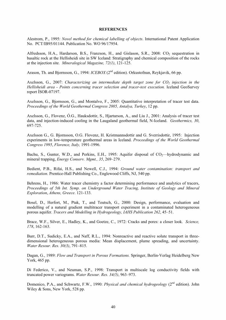
40
REFERENCES Alestrom, P., 1995: Novel method for chemical labelling of objects. International Patent Application No. PCT/IB95/01144. Publication No. WO 96/17954. Alfredsson, H.A., Hardarson, B.S., Franzson, H., and Gislason, S.R., 2008: CO2 sequestration in basaltic rock at the Hellisheidi site in SW Iceland: Stratigraphy and chemical composition of the rocks at the injection site. Mineralogical Magazine, 72(1), 121-125. Arason, Th. and Bjornsson, G., 1994: ICEBOX (2nd edition). Orkustofnun, Reykjavik, 66 pp. Axelsson, G., 2007: Characterizing an intermediate depth target zone for CO2 injection in the Hellisheidi area - Points concerning tracer selection and tracer-test execution. Iceland GeoSurvey report ÍSOR-07197. Axelsson, G., Bjornsson, G., and Montalvo, F., 2005: Quantitative interpretation of tracer test data. Proceedings of the World Geothermal Congress 2005, Antalya, Turkey, 12 pp. Axelsson, G., Flovenz, Ó.G., Hauksdottir, S., Hjartarson, A., and Liu J., 2001: Analysis of tracer test data, and injection-induced cooling in the Laugaland geothermal field, N-Iceland. Geothermics, 30, 697-725. Axelsson G., G. Bjornsson, O.G. Flovenz, H. Kristmannsdottir and G. Sverrisdottir, 1995: Injection experiments in low-temperature geothermal areas in Iceland. Proceedings of the World Geothermal Congress 1995, Florence, Italy, 1991-1996. Bachu, S., Gunter, W.D., and Perkins, E.H., 1995: Aquifer disposal of CO2—hydrodynamic and mineral trapping, Energy Conserv. Mgmt., 35, 269–279. Bedient, P.B., Rifai, H.S., and Newell, C.J., 1994: Ground water contamination: transport and remediation. Prentice-Hall Publishing Co., Englewood Cliffs, NJ, 540 pp. Behrens, H., 1986: Water tracer chemistry a factor determining performance and analytics of tracers, Proceedings of 5th Int. Symp. on Underground Water Tracing, Institute of Geology and Mineral Exploration, Athens, Greece. 121-133. Bosel, D., Herfort, M., Ptak, T., and Teutsch, G., 2000: Design, performance, evaluation and modelling of a natural gradient multitracer transport experiment in a contaminated heterogeneous porous aquifer. Tracers and Modelling in Hydrogeology, IAHS Publication 262, 45–51. Brace, W.F., Silver, E., Hadley, K., and Goetze, C., 1972: Cracks and pores: a closer look. Science, 178, 162-163. Burr, D.T., Sudicky, E.A., and Naff, R.L., 1994: Nonreactive and reactive solute transport in three-dimensional heterogeneous porous media: Mean displacement, plume spreading, and uncertainty. Water Resour. Res. 30(3), 791–815. Dagan, G., 1989: Flow and Transport in Porous Formations. Springer, Berlin-Verlag Heidelberg New York, 465 pp. Di Federico, V., and Neuman, S.P., 1998: Transport in multiscale log conductivity fields with truncated power variograms. Water Resour. Res. 34(5), 963–973. Domenico, P.A., and Schwartz, F.W., 1990: Physical and chemical hydrogeology (2nd edition). John Wiley & Sons, New York, 528 pp.
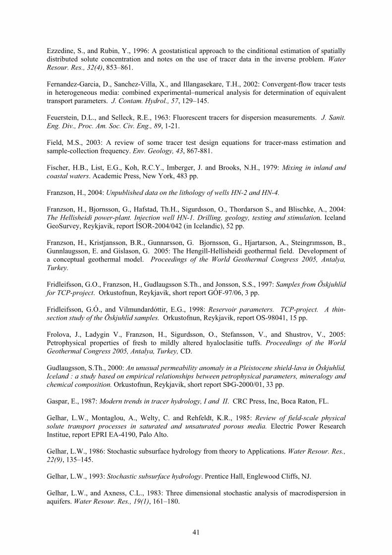
41
Ezzedine, S., and Rubin, Y., 1996: A geostatistical approach to the cinditional estimation of spatially distributed solute concentration and notes on the use of tracer data in the inverse problem. Water Resour. Res., 32(4), 853–861. Fernandez-Garcia, D., Sanchez-Villa, X., and Illangasekare, T.H., 2002: Convergent-flow tracer tests in heterogeneous media: combined experimental–numerical analysis for determination of equivalent transport parameters. J. Contam. Hydrol., 57, 129–145. Feuerstein, D.L., and Selleck, R.E., 1963: Fluorescent tracers for dispersion measurements. J. Sanit. Eng. Div., Proc. Am. Soc. Civ. Eng., 89, 1-21. Field, M.S., 2003: A review of some tracer test design equations for tracer-mass estimation and sample-collection frequency. Env. Geology, 43, 867-881. Fischer, H.B., List, E.G., Koh, R.C.Y., Imberger, J. and Brooks, N.H., 1979: Mixing in inland and coastal waters. Academic Press, New York, 483 pp. Franzson, H., 2004: Unpublished data on the lithology of wells HN-2 and HN-4. Franzson, H., Bjornsson, G., Hafstad, Th.H., Sigurdsson, O., Thordarson S., and Blischke, A., 2004: The Hellisheidi power-plant. Injection well HN-1. Drilling, geology, testing and stimulation. Iceland GeoSurvey, Reykjavik, report ÍSOR-2004/042 (in Icelandic), 52 pp. Franzson, H., Kristjansson, B.R., Gunnarsson, G. Bjornsson, G., Hjartarson, A., Steingrımsson, B., Gunnlaugsson, E. and Gislason, G. 2005: The Hengill-Hellisheidi geothermal field. Development of a conceptual geothermal model. Proceedings of the World Geothermal Congress 2005, Antalya, Turkey. Fridleifsson, G.O., Franzson, H., Gudlaugsson S.Th., and Jonsson, S.S., 1997: Samples from Öskjuhlíd for TCP-project. Orkustofnun, Reykjavik, short report GÓF-97/06, 3 pp. Fridleifsson, G.Ó., and Vilmundardóttir, E.G., 1998: Reservoir parameters. TCP-project. A thin-section study of the Öskjuhlíd samples. Orkustofnun, Reykjavik, report OS-98041, 15 pp. Frolova, J., Ladygin V., Franzson, H., Sigurdsson, O., Stefansson, V., and Shustrov, V., 2005: Petrophysical properties of fresh to mildly altered hyaloclasitie tuffs. Proceedings of the World Geothermal Congress 2005, Antalya, Turkey, CD. Gudlaugsson, S.Th., 2000: An unusual permeability anomaly in a Pleistocene shield-lava in Öskjuhlíd, Iceland : a study based on empirical relationships between petrophysical parameters, mineralogy and chemical composition. Orkustofnun, Reykjavik, short report SÞG-2000/01, 33 pp. Gaspar, E., 1987: Modern trends in tracer hydrology, I and II. CRC Press, Inc, Boca Raton, FL. Gelhar, L.W., Montaglou, A., Welty, C. and Rehfeldt, K.R., 1985: Review of field-scale physical solute transport processes in saturated and unsaturated porous media. Electric Power Research Institue, report EPRI EA-4190, Palo Alto. Gelhar, L.W., 1986: Stochastic subsurface hydrology from theory to Applications. Water Resour. Res., 22(9), 135–145. Gelhar, L.W., 1993: Stochastic subsurface hydrology. Prentice Hall, Englewood Cliffs, NJ. Gelhar, L.W., and Axness, C.L., 1983: Three dimensional stochastic analysis of macrodispersion in aquifers. Water Resour. Res., 19(1), 161–180.

42
Gelhar, L.W., Welty, C., and Rehfeldt, K.R., 1992: A critical review of data on field-scale dispersion in aquifers. Water Resour. Res., 28(7), 1955–1974. Gooddy, D.C., Darling, W.G., Abesser, C., and Lapworth, D.J., 2006: Using chlorofluorocarbons (CFCs) and sulphur hexafluoride (SF6) to characterize groundwater movement and residence time in a lowland Chalk catchment. Journal of Hydrology, 330, 44-52. Grathwohl, P., and Kleineidam, S., 1995: Impact of heterogeneous aquifer materials on sorption capacities and sorption dynamics of organic contaminants. Groundwater Quality: Remediation and Protection, IAHS Publ., 225, 79–86. Haggerty, R., Schroth, M.H., and Istok, J.D., 1998: Simplified method of push–pull test data analysis for determining in situ reaction rate coefficients. Ground Water, 36(2), 314–324. Hardarson, B.S., Helgadottir, H.M., and Franzson, H., 2007: The Hellisheidi power plant. Injection site beside Grauhnukar. Iceland GeoSurvey, Reykajvik, report ÍSOR-2007/001 (in Icelandic). Hauksdottir, S., Kristmannsdottir, H., Axelsson, G., Armannsson, H., Bjarnason, H., and Olafsson, M., 2000: The influence of effluent water discharged from the Namafjall geothermal field on local groundwater. Proceedings of the World Geothermal Congress 2000, Kyushu-Tohoku Japan, 603-608. Hitchen, B., 1996: Aquifer disposal of carbon dioxide, hydrologic and mineral trapping. Geoscience Publishing Sherwood Park, Alberta, Canada. Hohener, P., Werner, D., Balsiger, C., and Pasteris, G., 2003: Worldwide occurrence and fate of chlorofluorocarbons in groundwater. Crit. Rev. Env. Sci. Tec., 33, 1–29. Holloway, S., 1997: An overview of the underground disposal of carbon dioxide. Energy Convers. Manag., 38, 193–198. Istok, J.D., Humphrey, M.D., Schroth, M.H., Hyman, M.R., and O’Reilly, K.T., 1997: Single-Well, push pull test for in situ determination of microbial activities. Ground Water, 35(4), 619–631. Jonsson, S.S., Gudlaugsson, S.Th., Fridleifsson, G.O., Tulinius, H., and Steingrimsson, B., 1998: Reykjavík-area. wells HS-45 – HS-48. Geology and lithological logging. Orkustofnun, Reykjavik, report OS-98015 (in Icelandic), 30 pp. Kass W., 1998: Tracing technique in geohydrology. Balkema, Rotterdam. Klonis, N., Sawyer, W.H., 1996: Spectral properties of the prototropic forms of fluorescein in aqueous solution. J. Fluoresc., 6(3), 147-157. Leonhared, T H., Gordon, L., and Livingston, G., 1971: Acid-base equilibria of fluorescein and 2', 7'-dichlorofluorescein in their ground and fluorescent states. J. Phys. Chem., 75(2), 245-249. Lindqvist, L., 1960: A flash photolysis study of fluorescein. Ark. Kemi, 16, 79-138. Masters, G.M., and Wendell, P.E, 2007: Introduction to environmental engineering and science. Prentice-Hall Publishing Co., Englewood Cliffs, NJ, 708 pp. Miralles-Wilhelm, F., and Gelhar, L.W., 1996: Stochastic analysis of sorption macrokinetics in heterogeneous aquifers. Water Resour. Res. 32(6), 1541–1549. Miralles-Wilhelm, F., Gelhar, L.W., and Kapoor, V., 1997: Stochastic analysis of oxygen-limited biodegradation in three-dimensionally heterogeneous aquifers. Water Resour. Res., 33(6), 1251–1263.

43
Oelkers and Schott, 2005: Geochemical aspects of CO2 sequestration. Chemical Geology magazine 217, 183–186. Perkins, E.H., and Gunter, W.D., 1995: Aquifer disposal of CO2-rich greenhouse gases: Modeling of water–rock interaction paths in a siliciclastic aquifer. In: Kaharaka,Y.K., and Chudeav, O.V., (eds.): Water–Rock Interactions. Brookfield, Rotterdam, 895–898. Prinn, R.G., Weiss, R.F., Fraser, P.J., Simmonds, P.G., Cunnold, D.M., Alyea, F.N., O’Doherty, S., Salameh, P., Miller, B.R., Huang, J., Wang, R.H.J., Hartley, D.E., Harth, C., Steele, L.P., Sturrock, G., Midgley, P.M., and McCulloch, A., 2000: A history of chemically and radioactively important gases in air deduced from ALE/GAGE/AGAGE. J. Geophys. Res., 105, 17751–17792. Ptak, T., and Kleiner, K., 1998: Application of multilevel–multitracer transport experiments for the investigation of hydraulic and hydrogeochemical aquifer properties, Groundwater Quality: Remediation and Protection. IAHS Publication, 250, 343–351. Ptak, T., Schirmer, M., and Teutsch, G., 2000: Development and performance of a new multilevel groundwater sampling system. In: Wickramanayake, G.B., Gavaskar, A.R., Kelley, M.E., and Nehring, K.W. (Eds.): Risk, regulatory and monitoring considerations: remediation of chlorinated and recalcitrant compounds. Battelle Press, Columbus, 95–102. Ptak, T., and Schmid, G., 1996: Dual-tracer transport experiments in a physically and chemically heterogeneous porous aquifer: Effective transport parameters and spatial variability. J. Hydrol., 183(1-2), 117–138. Ptak, T., and Strobel, H., 1998: Sorption of fluorescent tracers in a physically and chemically heterogeneous aquifer material. In: Arehart, G.B., Hulston, J.R. (eds.): Water–rock interaction. Balkema, Rotterdam, 177–180. Ptak, T., Piepenbrink, M. and Martac, E., 2004: Tracer tests for the investigation of heterogeneous porous media and stochastic modelling of flow and transport—a review of some recent developments. Journal of Hydrology, 294, 122–163. Ragnarsson, A., 2003: Utilization of geothermal energy in Iceland. Proceedings of IGC 2003, Reykjavík, Iceland, 39-45. REN21, 2008: The global status report on renewable energy policy network for the 21st Century. Webpage : www.ren21.net. Rentier, C., Brouyere, S., and Dassargues, A., 2002: Integrating geophysical and tracer test data for accurate solute transport modeling in heterogeneous media. Groundwater Quality: Natural and Enhanced Restoration of Groundwater Pollution, IAHS Publication, 275, 3–10. Rose, P., Benoir, D., Lee, S.G., Tandia, B., and Kilbourn, P., 2000: Testing the naphthalene sulfonates as geothermal tracers at Dixie Valley, Ohaki and Awibengkok. Proceedings of the 25th Workshop on Geothermal Reservoir Engineering, Stanford University, Ca., 7 pp. Sabir, I.H., Torgersen, J., Haldorsen, S., and Aleström, P., 1999a: DNA tracers with information capacity and high detection sensitivity tested in groundwater studies. Hydrogeol. J., 7(3), 264–272. Sabir, I.H., Torgersen, J., Haldorsen, S., and Aleström, P., 1999b: DNA tracers with information capacity and high detection sensitivity tested in groundwater studies. Hydrogeol. J., 7(3), 264–272. Saemundsson, K., and Fridleifsson, G.O., 2003: Geological and geothermal maps of Hengill area, re-evaluation of the area south of Mt. Hengill (in Icelandic). Iceland GeoSurvey, Reykjavik, report ÍSOR-2003/020, 42 pp.

44
Saemundsson, K., Snorrason, S.P., and Fridleifsson, G.Ó., 1990: Geological map of the southern Hengill area, between Hengladalir and Krossfjöll (in Icelandic). Orkustofnun, Reykjavik, report OS-90008/JHD-02B, 15 pp. Sigurdsson, O., Gudmundsson, A., Fridleifsson G.O., Franzson, H., Gudlaugsson S.Th., and Stefansson, V., 2000: Database on Igneous Rock Properties in Icelandic Geothermal Systems. Status and Unexpected Results. Proceedings of the World Geothermal Congress 2000, Kyushu-Tohoku Japan, 2881-2886. Smart, P.L., and Laidlaw, I.M.S., 1977: An evaluation of some fluorescent dyes for water tracing. Water Resour. Res., 13, 15–33. Smith, S.A., and Pretorius, WA., 2002: The conservative behaviour of Fluorescein. Water SA, 28(4). Socolofsky, S.A., and Jirka, G.H., 2005: Lectures on special topics in mixing and transport processes in the environment engineering. Texas A&M University, Coastal and ocean engineering division, Texas. Sutton, D.J., Kabala, Z.J., Schaad, D.E., and Ruud, N.C., 2000: The dipole-flow test with a tracer: a new single-borehole tracer test for aquifer characterization. J. Contam. Hydrol., 44, 71–101. Tiedeman, C.R., and Hsieh, P.A., 2003: Evaluation of simulated forced gradient tracer tests in heterogeneous aquifers: different test types yield different longitudinal dispersivity estimates. In: Poeter, Zheng, Hill and Doherty (eds.): MODFLOW and MORE 2003—understanding through modelling. International Ground Water Modeling Center (IGWMC), Colorado School of Mines, 264– 268. Vert, M., Ptak, T., Biver, P., and Vittori, J., 1999: Geostatistical generation of three-dimensional aquifer realizations using the conditional SIS approach with direction trends imposed on variogram models. In: Gomez-Hernandez, J.J., et al. (Eds.): geoENV II—Geostatistics for environmental applications. Kluwer Academic, Dordrecht, 343–354. Wanninkhof, R., Ledwell, J.R., and Broecker, W.S., 1985: Gas exchange—wind speed relationship measured with sulfur hexafluoride on a lake. Science, 227, 1224–1226. Watson, J.D., Gilman, M., Witkowski, J., and Zoller, M., 1992: Recombinant DNA (2nd edition). WH Freeman, New York, 235 pp. Wilson, R.D., and Mackay, D.M., 1993: The use of SF6 as a conservative tracer in a saturated sandy media. Ground Water, 31, 719–724. Woodbury, A.D., and Rubin, Y., 2000: A full-Bayesian approach to parameter inference from tracer travel time moments and investigation of scale effects at the Cape Cod experimental site. Water Resour. Res, 36(1), 159–171. Zlotnik, V., Zurbuchen, B., Ptak, T., and Teutsch, G., 2000: Support volume and scale effect in hydraulic conductivity: Experimental aspects. In: Zhang, D., and Winter, C.L. (Eds.): Theory, modeling, and field investigation in hydrogeology: A special volume in honor of Shlomo P. Neuman’s 60th birthday. Geological Society of America, Boulder, Colorado, Special Paper, 348, 215–231. Zoellmann, K., Kinzelbach, W., and Fulda, C., 2001: Environmental tracer transport (3H and SF6) in the saturated and unsaturated zones and its use in nitrate pollution management. Journal of Hydrology, 240 (3-4), 187-205.