Embed Size (px)
Citation preview

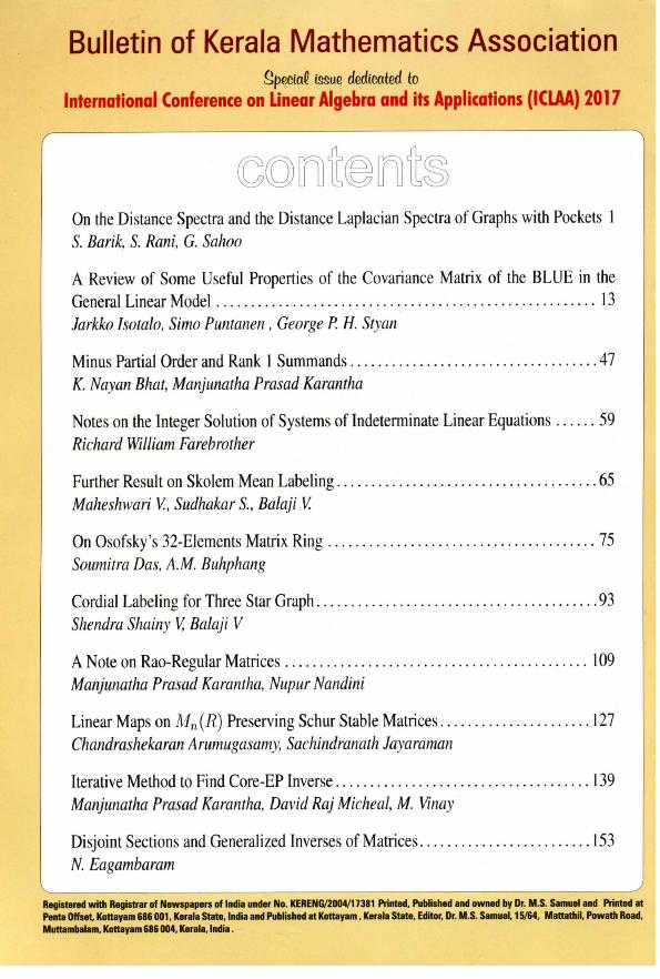
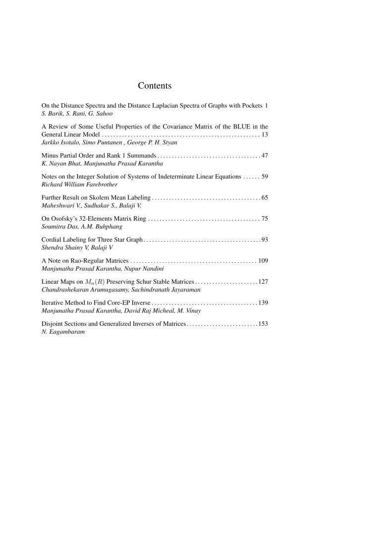
Contents
On the Distance Spectra and the Distance Laplacian Spectra of Graphs with Pockets 1
S. Barik, S. Rani, G. Sahoo
A Review of Some Useful Properties of the Covariance Matrix of the BLUE in the
General Linear Model . . . . . . . . . . . . . . . . . . . . . . . . . . . . . . . . . . . . . . . . . . . . . . . . . . . . . . . 13
Jarkko Isotalo, Simo Puntanen , George P. H. Styan
Minus Partial Order and Rank 1 Summands . . . . . . . . . . . . . . . . . . . . . . . . . . . . . . . . . . . . 47
K. Nayan Bhat, Manjunatha Prasad Karantha
Notes on the Integer Solution of Systems of Indeterminate Linear Equations . . . . . . 59
Richard William Farebrother
Further Result on Skolem Mean Labeling . . . . . . . . . . . . . . . . . . . . . . . . . . . . . . . . . . . . . . 65
Maheshwari V., Sudhakar S., Balaji V.
On Osofsky’s 32-Elements Matrix Ring . . . . . . . . . . . . . . . . . . . . . . . . . . . . . . . . . . . . . . . 75
Soumitra Das, A.M. Buhphang
Cordial Labeling for Three Star Graph . . . . . . . . . . . . . . . . . . . . . . . . . . . . . . . . . . . . . . . . . 93
Shendra Shainy V, Balaji V
A Note on Rao-Regular Matrices . . . . . . . . . . . . . . . . . . . . . . . . . . . . . . . . . . . . . . . . . . . . 109
Manjunatha Prasad Karantha, Nupur Nandini
Linear Maps on Mn(R) Preserving Schur Stable Matrices . . . . . . . . . . . . . . . . . . . . . . 127
Chandrashekaran Arumugasamy, Sachindranath Jayaraman
Iterative Method to Find Core-EP Inverse . . . . . . . . . . . . . . . . . . . . . . . . . . . . . . . . . . . . . 139
Manjunatha Prasad Karantha, David Raj Micheal, M. Vinay
Disjoint Sections and Generalized Inverses of Matrices. . . . . . . . . . . . . . . . . . . . . . . . .153
N. Eagambaram

Preface
International conference on Linear Algebra and its Applications–ICLAA 2017,
third in its sequence, following CMTGIM 2012 and ICLAA 2014, held in Manipal
Academy of Higher Education, Manipal, India in December 11-15, 2017.
Like its preceding conferences, ICLAA 2017 is also focused on the theory of
Linear Algebra and Matrix Theory, and their applications in Statistics, Network Theory
and in other branches of sciences. Study of Covariance Matrices, being part of Matrix
Method in Statistics, has applications in various branches of sciences. It plays crucial
role in the study of measurement of uncertainty and naturally in the study of Nuclear
Data. Theme meeting, which initially planned to be a preconference meeting, further
progressed into an independent event parallel to ICLAA 2017, involving discussion on
different methodology of generating the covariance information, training modules on
different techniques and deliberations on presenting new research.
About 167 delegates have registered for ICLAA 2017 alone (37 Invited+ 75 Con-
tributory + 04 Poster) and are from 17 different countries of the world. Interestingly,
more than 80% are repeaters from the earlier conference and the remaining 20% are
young students or scholars. In spite of a few dropouts due to unavoidable constraints,
it is felt evident that the group of scholars with focus area of Linear Algebra, Matrix
Methods in Statistics and Matrices and Graphs are not only consolidating, also grow-
ing as a society with a strong bond. ICLAA 2017 provided a platform for renowned
Mathematicians and Statisticians to come together and discuss research problems, it
provided ample of time for young scholars to present their contribution before eminent
scholars. Every contributory speaker got not less than thirty minutes to present their re-
sults. Also, ICLAA 2017 was with several special lectures from senior scientists aimed
at encouraging young scholars.
The sponsors of ICLAA 2017 are NBHM, SERB, CSIR and ICTP. Dr. Ebrahim
Ghorbani and Dr. Zheng Bing are the two international participants benifited from
ICTP grant for their international travel.
The conference was opened with an informal welcome and opening remark by K.
Manjunatha Prasad (Organizing Secretary) and R. B. Bapat (Chairman, Scientific Com-
mittee). Invited talks and the special lectures were organized in 13 different sessions
and contributory talks in 17 sessions. Poster presentation was arranged on December
12, 2017.
In an informal discussion, it has been consented by the present scientific commit-
tee and the organizing committee members that
(i) MAHE would continue to organize ICLAA 2020 in December 2020, the fourth
in its sequence
(ii) Manjunatha Prasad would put up a proposal to organize ILAS conference in the
earliest possible occasion (2022/23), in consultation with Kirkland

(iii) Manjunatha Prasad to initiate a dialog with the members in the present network
to have Indian Society for Linear Algebra and its Application
The organizers are very proud of bringing out two special issues related to the
conference, the one with Bulletin of Kerala Mathematics Association and the other one
with Special Matrices (De Gruyter). The organizers are thankful to managerial team of
BKMA, particularly Samuel Mattathil, and the chief editor Carlos Martins da Fonseca
of Special Matrices for their kind support in bringing up these special issues. They are
also thankful to all the authors for submitting their articles and reviewers for sparing
their valuable time.
Ravindra B Bapat, ISI, Delhi, India
Steve Kirkland, University of Manitoba, Canada
K. Manjunatha Prasad, MAHE, Manipal, India
Simo Puntanen, University of Tampere, Finland
Bulletin of Kerala Mathematics Association, Special Issue
Vol. 16, No. 1 (2018, June) 13–45
A REVIEW OF SOME USEFUL PROPERTIES OF
THE COVARIANCE MATRIX OF THE BLUE IN
THE GENERAL LINEAR MODEL
Jarkko Isotalo∗, Simo Puntanen1∗∗, George P. H. Styan∗∗∗
∗Department of Forest Sciences,
University of Helsinki, [email protected]
∗∗Faculty of Natural Sciences,
University of Tampere, [email protected]
∗∗∗Department of Mathematics and Statistics,
McGill University, Montreal, Canada
(Received 05.02.2018; Accepted 01.03.2018)
Abstract. In this paper we consider the linear statistical model y = Xβ+ε, which
can be shortly denoted as the tripletM = y,Xβ,V. Here X is a known n × pfixed model matrix, the vector y is an observable n-dimensional random vector, β
is a p × 1 vector of fixed but unknown parameters, and ε is an unobservable vector
of random errors with expectation E(ε) = 0, and covariance matrix cov(ε) =V, where the nonnegative definite matrix V is known. In our considerations it is
essential that the covariance matrix V is known; if this is not the case the statistical
considerations become much more complicated.
Our main focus is to define and introduce, in the general form, without rank
conditions, the key properties of the best linear unbiased estimator, BLUE, of Xβ.
In particular we consider some specific properties of the covariance matrix of the
BLUE. We also deal shortly with the best linear unbiased predictor, BLUP, of y∗,
when y∗ is assumed to come from y∗ = X∗β + ε∗, where X∗ is a known matrix,
β is the same vector of unknown parameters as in M , and ε∗ is a q-dimensional
random error vector. This article is of review type, providing easy-to-read collection
of useful results concerning specific properties of the covariance matrix of the BLUE.
Most results appear in literature but our aim is to create a convenient “package” of
some essential results.
14 Jarkko Isotalo, Simo Puntanen , George P. H. Styan
Keywords: BLUE, BLUP, covariance matrix, linear statistical model, Lowner par-
tial ordering, generalized inverse.
Classification: 62J05; 62J10
1. Introduction
We will consider the general linear model
y = Xβ + ε , or shortly the tripletM = y,Xβ,V , (1.1)
where X is a known n× p model matrix, the vector y is an observable n-dimensional
random vector (so-called response vector), β is p-dimensional vector of unknown but
fixed parameters, and ε is an unobservable vector of random errors with expectation
E(ε) = 0, and covariance matrix cov(ε) = V. Often the covariance matrix is of the
type cov(ε) = σ2V, where σ2 is an unknown nonzero constant. However, in most
of our considerations σ2 has no role and in such cases we omit it. The nonnegative
definite matrix V is known and can be singular. The set of nonnegative definite n× nmatrices is denoted as NNDn.
As the covariance matrix is so central concept for our considerations, we might
recall that underM it is defined as
V = cov(y) = E(y − µ)(y − µ)′, where µ = Xβ = E(y) , (1.2)
and ′ denotes the transpose of the matrix argument. Thus obviously,
cov(Ay) = AVA′, (1.3)
where A ∈ Rm×n, the set of m × n real matrices. Instead of “covariance matrix”,
some authors use the name “variance-covariance matrix” or “dispersion matrix”. The
cross-covariance matrix between random vectors u and v is defined as
cov(u,v) = E[u− E(u)][v − E(v)]′. (1.4)
Then some words about the notation. The symbols A−, A+, C (A), and C (A)⊥,
denote, respectively, a generalized inverse, the (unique) Moore–Penrose inverse, the
column space, and the orthogonal complement of the column space of the matrix A.
The Moore–Penrose inverse A+ is defined as a unique matrix satisfying the following
four conditions:
AA+A = A, A+AA+ = A+, (AA+)′ = AA+, (A+A)′ = A+A. (1.5)
1 Corresponding author
Properties of the BLUE’s covariance matrix 15
Notation A− refers to any matrix satisfying AA−A = A. By (A : B) we denote the
partitioned matrix with Aa×b and Ba×c as submatrices. The symbol A⊥ stands for
any matrix satisfying C (A⊥) = C (A)⊥. Furthermore, we will use PA = AA+ =A(A′A)−A′ to denote the orthogonal projector (with respect to the standard inner
product) onto the column space C (A), and QA = I − PA, where I refers to the
identity matrix of conformable dimension. In particular, it appears to be useful to
denote
H = PX , M = In −PX , (1.6)
in which case, for any vector y ∈ Rn,
minµ∈C (X)
‖y − µ‖2 = minβ‖y −Xβ‖2 = ‖y − µ‖2 = y′My , (1.7)
where µ = Hy = Xβ, with β being any (least-squares) solution to so-called normal
equation
X′Xβ = X′y . (1.8)
Notice that in (1.7) and (1.8) we use y, β, β and µ as “merely mathematical” vectors,
not random vectors nor parameters of the modelM .
The notation PX;V−1 , where V is positive definite, refers to the orthogonal pro-
jector onto C (X) with respect to the inner product matrix V−1, i.e.,
minµ∈C (X)
(y − µ)′V−1(y − µ) = minβ‖y −Xβ‖2
V−1 = ‖y − µ‖2V−1 , (1.9)
where ‖a‖2V−1 = a′V−1a for a ∈ Rn, and
µ = Xβ = PX;V−1y = X(X′V−1X)−X′V−1y , (1.10)
with β being any solution to the generalized normal equation
X′V−1Xβ = X′V−1y . (1.11)
We shall concentrate on the linear unbiased estimators, LUEs, and hence we need
the concept of estimability. The parametric function η = Kβ, where K ∈ Rq×p, is
estimable underM if and only if there exists a matrix B ∈ Rq×n such that
E(By) = BXβ = Kβ for all β ∈ Rp, i.e., BX = K . (1.12)
Such a matrix B exists only when
C (K′) ⊂ C (X′) , (1.13)
which, therefore, is the condition for η = Kβ to be estimable. The LUE By is the best
linear unbiased estimator, BLUE, of estimable Kβ if By has the smallest covariance
matrix in the Lowner sense among all linear unbiased estimators of Kβ:
cov(By) ≤L cov(B#y) for all B# : B#X = K , (1.14)
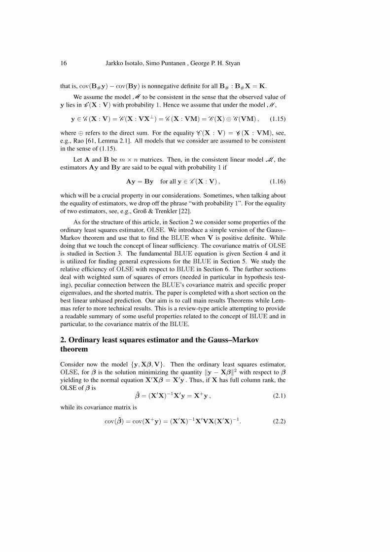
16 Jarkko Isotalo, Simo Puntanen , George P. H. Styan
that is, cov(B#y)− cov(By) is nonnegative definite for all B# : B#X = K.
We assume the modelM to be consistent in the sense that the observed value of
y lies in C (X : V) with probability 1. Hence we assume that under the modelM ,
y ∈ C (X : V) = C (X : VX⊥) = C (X : VM) = C (X)⊕ C (VM) , (1.15)
where ⊕ refers to the direct sum. For the equality C (X : V) = C (X : VM), see,
e.g., Rao [61, Lemma 2.1]. All models that we consider are assumed to be consistent
in the sense of (1.15).
Let A and B be m × n matrices. Then, in the consistent linear model M , the
estimators Ay and By are said to be equal with probability 1 if
Ay = By for all y ∈ C (X : V) , (1.16)
which will be a crucial property in our considerations. Sometimes, when talking about
the equality of estimators, we drop off the phrase “with probability 1”. For the equality
of two estimators, see, e.g., Groß & Trenkler [22].
As for the structure of this article, in Section 2 we consider some properties of the
ordinary least squares estimator, OLSE. We introduce a simple version of the Gauss–
Markov theorem and use that to find the BLUE when V is positive definite. While
doing that we touch the concept of linear sufficiency. The covariance matrix of OLSEis studied in Section 3. The fundamental BLUE equation is given Section 4 and it
is utilized for finding general expressions for the BLUE in Section 5. We study the
relative efficiency of OLSE with respect to BLUE in Section 6. The further sections
deal with weighted sum of squares of errors (needed in particular in hypothesis test-
ing), peculiar connection between the BLUE’s covariance matrix and specific proper
eigenvalues, and the shorted matrix. The paper is completed with a short section on the
best linear unbiased prediction. Our aim is to call main results Theorems while Lem-
mas refer to more technical results. This is a review-type article attempting to provide
a readable summary of some useful properties related to the concept of BLUE and in
particular, to the covariance matrix of the BLUE.
2. Ordinary least squares estimator and the Gauss–Markov
theorem
Consider now the model y,Xβ,V. Then the ordinary least squares estimator,
OLSE, for β is the solution minimizing the quantity ‖y − Xβ‖2 with respect to β
yielding to the normal equation X′Xβ = X′y . Thus, if X has full column rank, the
OLSE of β is
β = (X′X)−1X′y = X+y , (2.1)
while its covariance matrix is
cov(β) = cov(X+y) = (X′X)−1X′VX(X′X)−1. (2.2)
Properties of the BLUE’s covariance matrix 17
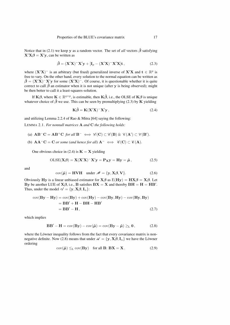
Notice that in (2.1) we keep y as a random vector. The set of all vectors β satisfying
X′Xβ = X′y, can be written as
β = (X′X)−X′y + [Ip − (X′X)−X′X]t , (2.3)
where (X′X)− is an arbitrary (but fixed) generalized inverse of X′X and t ∈ Rp is
free to vary. On the other hand, every solution to the normal equation can be written as
β = (X′X)−X′y for some (X′X)−. Of course, it is questionable whether it is quite
correct to call β an estimator when it is not unique (after y is being observed); might
be then better to call it a least-squares-solution.
If Kβ, where K ∈ Rq×p, is estimable, then Kβ, i.e., the OLSE of Kβ is unique
whatever choice of β we use. This can be seen by premultiplying (2.3) by K yielding
Kβ = K(X′X)−X′y , (2.4)
and utilizing Lemma 2.2.4 of Rao & Mitra [64] saying the following:
LEMMA 2.1. For nonnull matrices A and C the following holds:
(a) AB−C = AB+C for all B− ⇐⇒ C (C) ⊂ C (B) & C (A′) ⊂ C (B′).
(b) AA−C = C or some (and hence for all) A− ⇐⇒ C (C) ⊂ C (A).
One obvious choice in (2.4) is K = X yielding
OLSE(Xβ) = X(X′X)−X′y = PXy = Hy = µ , (2.5)
and
cov(µ) = HVH underM = y,Xβ,V. (2.6)
Obviously Hy is a linear unbiased estimator for Xβ as E(Hy) = HXβ = Xβ. Let
By be another LUE of Xβ, i.e., B satisfies BX = X and thereby BH = H = HB′.
Thus, under the model A = y,Xβ, In:
cov(By −Hy) = cov(By) + cov(Hy)− cov(By,Hy)− cov(Hy,By)
= BB′ +H−BH−HB′
= BB′ −H , (2.7)
which implies
BB′ −H = cov(By)− cov(µ) = cov(By − µ) ≥L 0 , (2.8)
where the Lowner inequality follows from the fact that every covariance matrix is non-
negative definite. Now (2.8) means that under A = y,Xβ, In we have the Lowner
ordering
cov(µ) ≤L cov(By) for all B: BX = X . (2.9)
18 Jarkko Isotalo, Simo Puntanen , George P. H. Styan
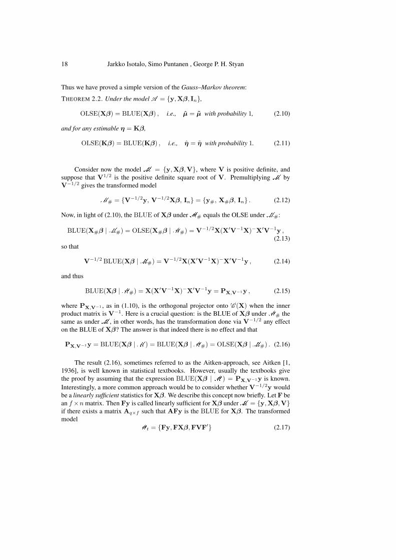
Thus we have proved a simple version of the Gauss–Markov theorem:
THEOREM 2.2. Under the model A = y,Xβ, In,
OLSE(Xβ) = BLUE(Xβ) , i.e., µ = µ with probability 1, (2.10)
and for any estimable η = Kβ,
OLSE(Kβ) = BLUE(Kβ) , i.e., η = η with probability 1. (2.11)
Consider now the model M = y,Xβ,V, where V is positive definite, and
suppose that V1/2 is the positive definite square root of V. Premultiplying M by
V−1/2 gives the transformed model
M# = V−1/2y, V−1/2Xβ, In = y#, X#β, In . (2.12)
Now, in light of (2.10), the BLUE of Xβ underM# equals the OLSE underM#:
BLUE(X#β |M#) = OLSE(X#β |M#) = V−1/2X(X′V−1X)−X′V−1y ,(2.13)
so that
V−1/2 BLUE(Xβ |M#) = V−1/2X(X′V−1X)−X′V−1y , (2.14)
and thus
BLUE(Xβ |M#) = X(X′V−1X)−X′V−1y = PX,V−1y , (2.15)
where PX,V−1 , as in (1.10), is the orthogonal projector onto C (X) when the inner
product matrix is V−1. Here is a crucial question: is the BLUE of Xβ underM# the
same as under M , in other words, has the transformation done via V−1/2 any effect
on the BLUE of Xβ? The answer is that indeed there is no effect and that
PX,V−1y = BLUE(Xβ |M ) = BLUE(Xβ |M#) = OLSE(Xβ |M#) . (2.16)
The result (2.16), sometimes referred to as the Aitken-approach, see Aitken [1,
1936], is well known in statistical textbooks. However, usually the textbooks give
the proof by assuming that the expression BLUE(Xβ | M ) = PX,V−1y is known.
Interestingly, a more common approach would be to consider whether V−1/2y would
be a linearly sufficient statistics for Xβ. We describe this concept now briefly. Let F be
an f×n matrix. Then Fy is called linearly sufficient for Xβ underM = y,Xβ,Vif there exists a matrix Aq×f such that AFy is the BLUE for Xβ. The transformed
model
Mt = Fy,FXβ,FVF′ (2.17)
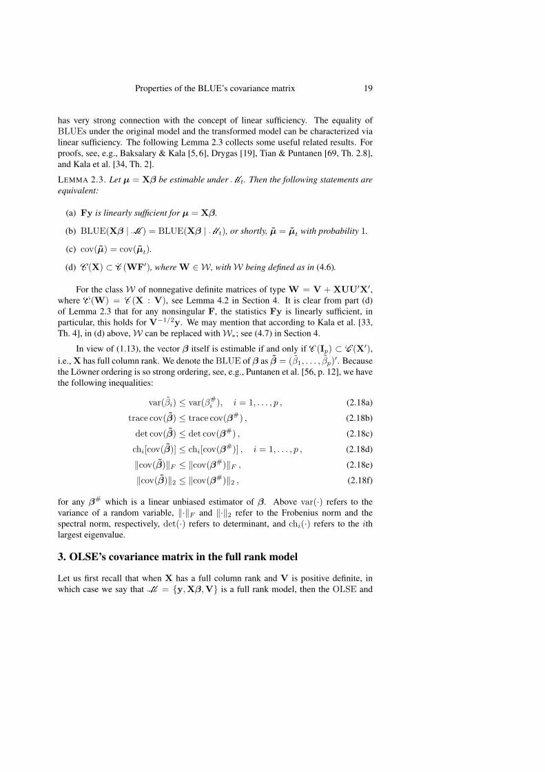
Properties of the BLUE’s covariance matrix 19
has very strong connection with the concept of linear sufficiency. The equality of
BLUEs under the original model and the transformed model can be characterized via
linear sufficiency. The following Lemma 2.3 collects some useful related results. For
proofs, see, e.g., Baksalary & Kala [5, 6], Drygas [19], Tian & Puntanen [69, Th. 2.8],
and Kala et al. [34, Th. 2].
LEMMA 2.3. Let µ = Xβ be estimable underMt. Then the following statements are
equivalent:
(a) Fy is linearly sufficient for µ = Xβ.
(b) BLUE(Xβ |M ) = BLUE(Xβ |Mt), or shortly, µ = µt with probability 1.
(c) cov(µ) = cov(µt).
(d) C (X) ⊂ C (WF′), where W ∈ W , withW being defined as in (4.6).
For the class W of nonnegative definite matrices of type W = V + XUU′X′,
where C (W) = C (X : V), see Lemma 4.2 in Section 4. It is clear from part (d)
of Lemma 2.3 that for any nonsingular F, the statistics Fy is linearly sufficient, in
particular, this holds for V−1/2y. We may mention that according to Kala et al. [33,
Th. 4], in (d) above,W can be replaced withW∗; see (4.7) in Section 4.
In view of (1.13), the vector β itself is estimable if and only if C (Ip) ⊂ C (X′),
i.e., X has full column rank. We denote the BLUE of β as β = (β1, . . . , βp)′. Because
the Lowner ordering is so strong ordering, see, e.g., Puntanen et al. [56, p. 12], we have
the following inequalities:
var(βi) ≤ var(β#i ), i = 1, . . . , p , (2.18a)
trace cov(β) ≤ trace cov(β#) , (2.18b)
det cov(β) ≤ det cov(β#) , (2.18c)
chi[cov(β)] ≤ chi[cov(β#)] , i = 1, . . . , p , (2.18d)
‖cov(β)‖F ≤ ‖cov(β#)‖F , (2.18e)
‖cov(β)‖2 ≤ ‖cov(β#)‖2 , (2.18f)
for any β# which is a linear unbiased estimator of β. Above var(·) refers to the
variance of a random variable, ‖·‖F and ‖·‖2 refer to the Frobenius norm and the
spectral norm, respectively, det(·) refers to determinant, and chi(·) refers to the ithlargest eigenvalue.
3. OLSE’s covariance matrix in the full rank model
Let us first recall that when X has a full column rank and V is positive definite, in
which case we say that M = y,Xβ,V is a full rank model, then the OLSE and
20 Jarkko Isotalo, Simo Puntanen , George P. H. Styan
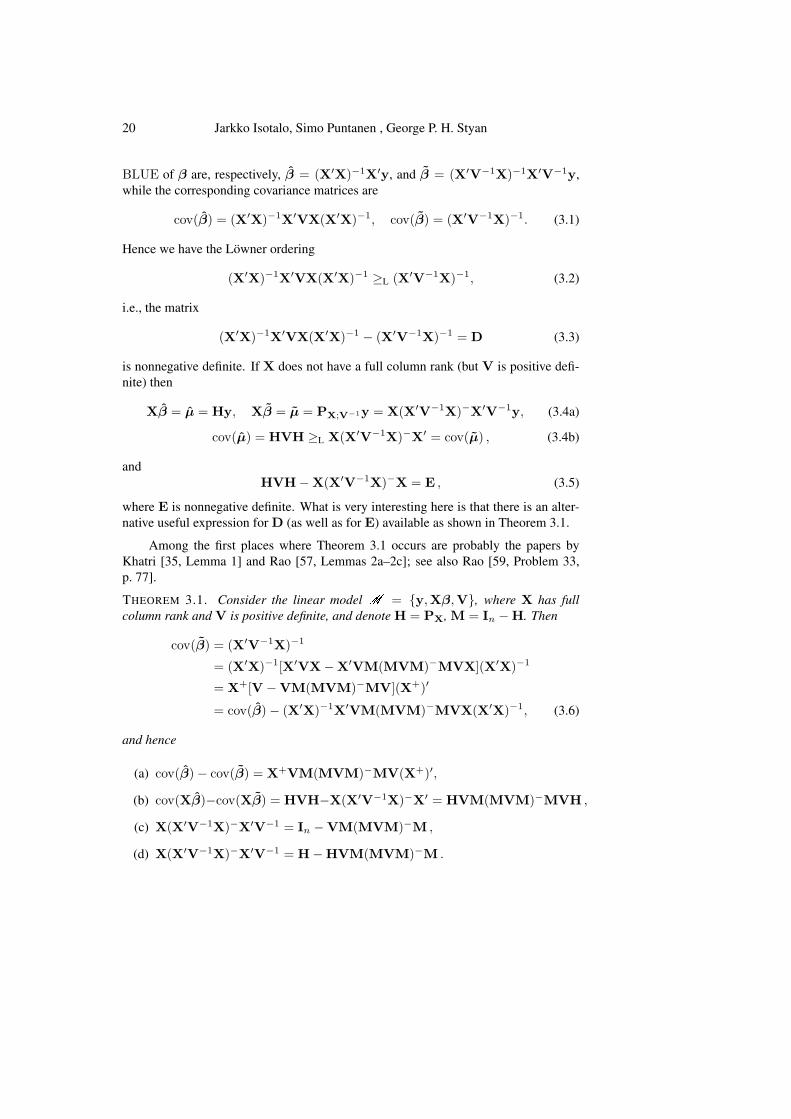
BLUE of β are, respectively, β = (X′X)−1X′y, and β = (X′V−1X)−1X′V−1y,
while the corresponding covariance matrices are
cov(β) = (X′X)−1X′VX(X′X)−1, cov(β) = (X′V−1X)−1. (3.1)
Hence we have the Lowner ordering
(X′X)−1X′VX(X′X)−1 ≥L (X′V−1X)−1, (3.2)
i.e., the matrix
(X′X)−1X′VX(X′X)−1 − (X′V−1X)−1 = D (3.3)
is nonnegative definite. If X does not have a full column rank (but V is positive defi-
nite) then
Xβ = µ = Hy, Xβ = µ = PX;V−1y = X(X′V−1X)−X′V−1y, (3.4a)
cov(µ) = HVH ≥L X(X′V−1X)−X′ = cov(µ) , (3.4b)
and
HVH−X(X′V−1X)−X = E , (3.5)
where E is nonnegative definite. What is very interesting here is that there is an alter-
native useful expression for D (as well as for E) available as shown in Theorem 3.1.
Among the first places where Theorem 3.1 occurs are probably the papers by
Khatri [35, Lemma 1] and Rao [57, Lemmas 2a–2c]; see also Rao [59, Problem 33,
p. 77].
THEOREM 3.1. Consider the linear model M = y,Xβ,V, where X has full
column rank and V is positive definite, and denote H = PX, M = In −H. Then
cov(β) = (X′V−1X)−1
= (X′X)−1[X′VX−X′VM(MVM)−MVX](X′X)−1
= X+[V −VM(MVM)−MV](X+)′
= cov(β)− (X′X)−1X′VM(MVM)−MVX(X′X)−1, (3.6)
and hence
(a) cov(β)− cov(β) = X+VM(MVM)−MV(X+)′,
(b) cov(Xβ)−cov(Xβ) = HVH−X(X′V−1X)−X′ = HVM(MVM)−MVH ,
(c) X(X′V−1X)−X′V−1 = In −VM(MVM)−M ,
(d) X(X′V−1X)−X′V−1 = H−HVM(MVM)−M .
Properties of the BLUE’s covariance matrix 21
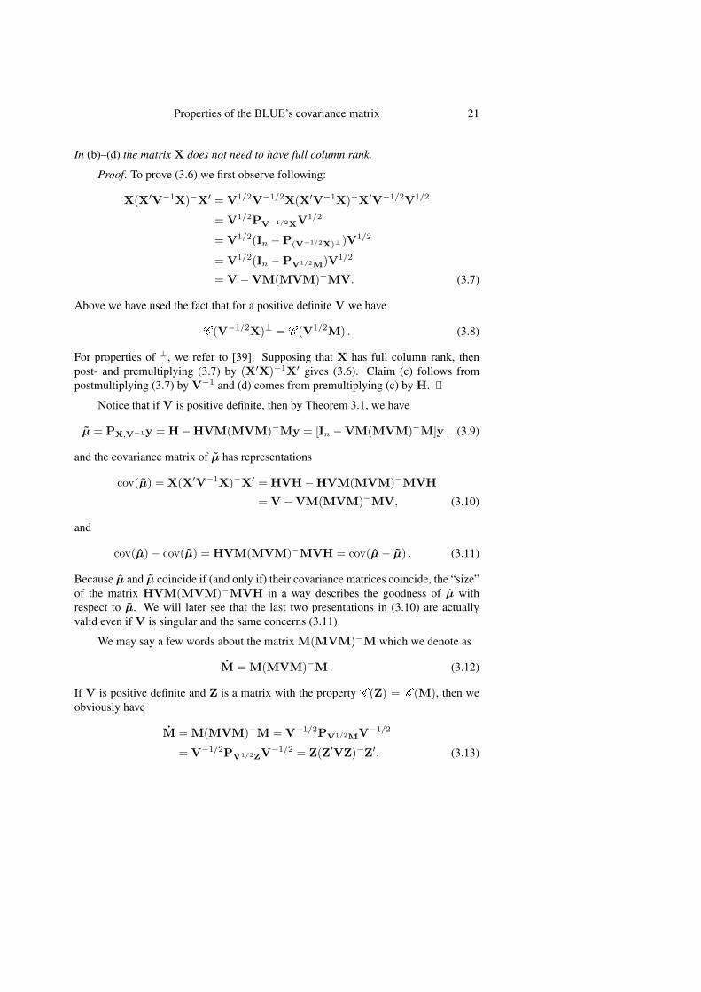
In (b)–(d) the matrix X does not need to have full column rank.
Proof. To prove (3.6) we first observe following:
X(X′V−1X)−X′ = V1/2V−1/2X(X′V−1X)−X′V−1/2V1/2
= V1/2PV−1/2XV1/2
= V1/2(In −P(V−1/2X)⊥)V1/2
= V1/2(In −PV1/2M)V1/2
= V −VM(MVM)−MV. (3.7)
Above we have used the fact that for a positive definite V we have
C (V−1/2X)⊥ = C (V1/2M) . (3.8)
For properties of ⊥, we refer to [39]. Supposing that X has full column rank, then
post- and premultiplying (3.7) by (X′X)−1X′ gives (3.6). Claim (c) follows from
postmultiplying (3.7) by V−1 and (d) comes from premultiplying (c) by H.
Notice that if V is positive definite, then by Theorem 3.1, we have
µ = PX;V−1y = H−HVM(MVM)−My = [In −VM(MVM)−M]y , (3.9)
and the covariance matrix of µ has representations
cov(µ) = X(X′V−1X)−X′ = HVH−HVM(MVM)−MVH
= V −VM(MVM)−MV, (3.10)
and
cov(µ)− cov(µ) = HVM(MVM)−MVH = cov(µ− µ) . (3.11)
Because µ and µ coincide if (and only if) their covariance matrices coincide, the “size”
of the matrix HVM(MVM)−MVH in a way describes the goodness of µ with
respect to µ. We will later see that the last two presentations in (3.10) are actually
valid even if V is singular and the same concerns (3.11).
We may say a few words about the matrix M(MVM)−M which we denote as
M = M(MVM)−M . (3.12)
If V is positive definite and Z is a matrix with the property C (Z) = C (M), then we
obviously have
M = M(MVM)−M = V−1/2PV1/2MV−1/2
= V−1/2PV1/2ZV−1/2 = Z(Z′VZ)−Z′, (3.13)
22 Jarkko Isotalo, Simo Puntanen , George P. H. Styan
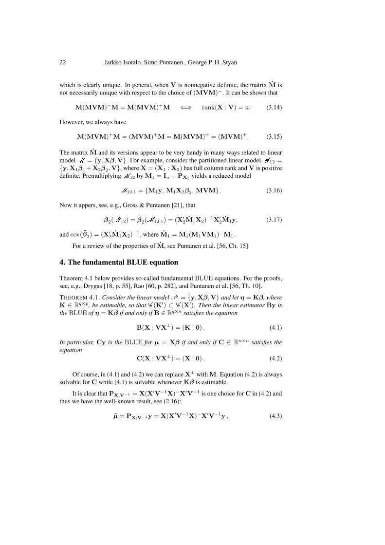
which is clearly unique. In general, when V is nonnegative definite, the matrix M is
not necessarily unique with respect to the choice of (MVM)−. It can be shown that
M(MVM)−M = M(MVM)+M ⇐⇒ rank(X : V) = n. (3.14)
However, we always have
M(MVM)+M = (MVM)+M = M(MVM)+ = (MVM)+. (3.15)
The matrix M and its versions appear to be very handy in many ways related to linear
modelM = y,Xβ,V. For example, consider the partitioned linear modelM12 =y,X1β1+X2β2,V, where X = (X1 : X2) has full column rank and V is positive
definite. PremultiplyingM12 by M1 = In −PX1yields a reduced model
M12·1 = M1y, M1X2β2, MVM . (3.16)
Now it appers, see, e.g., Gross & Puntanen [21], that
β2(M12) = β2(M12·1) = (X′2M1X2)
−1X′2M1y, (3.17)
and cov(β2) = (X′2M1X2)
−1, where M1 = M1(M1VM1)−M1.
For a review of the properties of M, see Puntanen et al. [56, Ch. 15].
4. The fundamental BLUE equation
Theorem 4.1 below provides so-called fundamental BLUE equations. For the proofs,
see, e.g., Drygas [18, p. 55], Rao [60, p. 282], and Puntanen et al. [56, Th. 10].
THEOREM 4.1. Consider the linear modelM = y,Xβ,V and let η = Kβ, where
K ∈ Rq×p, be estimable, so that C (K′) ⊂ C (X′). Then the linear estimator By is
the BLUE of η = Kβ if and only if B ∈ Rq×n satisfies the equation
B(X : VX⊥) = (K : 0) . (4.1)
In particular, Cy is the BLUE for µ = Xβ if and only if C ∈ Rn×n satisfies the
equation
C(X : VX⊥) = (X : 0) . (4.2)
Of course, in (4.1) and (4.2) we can replace X⊥ with M. Equation (4.2) is always
solvable for C while (4.1) is solvable whenever Kβ is estimable.
It is clear that PX;V−1 = X(X′V−1X)−X′V−1 is one choice for C in (4.2) and
thus we have the well-known result, see (2.16):
µ = PX;V−1y = X(X′V−1X)−X′V−1y . (4.3)
Properties of the BLUE’s covariance matrix 23
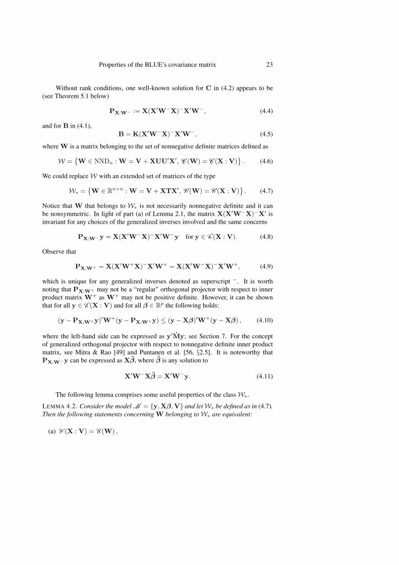
Without rank conditions, one well-known solution for C in (4.2) appears to be
(see Theorem 5.1 below)
PX;W− := X(X′W−X)−X′W−, (4.4)
and for B in (4.1),
B = K(X′W−X)−X′W−, (4.5)
where W is a matrix belonging to the set of nonnegative definite matrices defined as
W =W ∈ NNDn : W = V +XUU′X′, C (W) = C (X : V)
. (4.6)
We could replaceW with an extended set of matrices of the type
W∗ =W ∈ Rn×n : W = V +XTX′, C (W) = C (X : V)
. (4.7)
Notice that W that belongs to W∗ is not necessarily nonnegative definite and it can
be nonsymmetric. In light of part (a) of Lemma 2.1, the matrix X(X′W−X)−X′ is
invariant for any choices of the generalized inverses involved and the same concerns
PX;W−y = X(X′W−X)−X′W−y for y ∈ C (X : V). (4.8)
Observe that
PX;W+ = X(X′W+X)−X′W+ = X(X′W−X)−X′W+, (4.9)
which is unique for any generalized inverses denoted as superscript −. It is worth
noting that PX;W+ may not be a “regular” orthogonal projector with respect to inner
product matrix W+ as W+ may not be positive definite. However, it can be shown
that for all y ∈ C (X : V) and for all β ∈ Rp the following holds:
(y −PX;W+y)′W+(y −PX;W+y) ≤ (y −Xβ)′W+(y −Xβ) , (4.10)
where the left-hand side can be expressed as y′My; see Section 7. For the concept
of generalized orthogonal projector with respect to nonnegative definite inner product
matrix, see Mitra & Rao [49] and Puntanen et al. [56, §2.5]. It is noteworthy that
PX;W−y can be expressed as Xβ, where β is any solution to
X′W−Xβ = X′W−y. (4.11)
The following lemma comprises some useful properties of the classW∗.
LEMMA 4.2. Consider the modelM = y,Xβ,V and letW∗ be defined as in (4.7).
Then the following statements concerning W belonging toW∗ are equivalent:
(a) C (X : V) = C (W) ,
24 Jarkko Isotalo, Simo Puntanen , George P. H. Styan
(b) C (X) ⊂ C (W) ,
(c) X′W−X is invariant for any choice of W−,
(d) C (X′W−X) = C (X′) for any choice of W−,
(e) X(X′W−X)−X′W−X = X for any choices of W− and (X′W−X)−.
Moreover, each of these statements is equivalent also to C (X : V) = C (W′),and hence to the statements (b)–(e) by replacing W with W′.
Observe that obviously C (W) = C (W′) and that the invariance properties in (d)
and (e) concern not only the the choice of the generalized inverse of W but also the
choice of W ∈ W∗. For further properties ofW∗, see, e.g., Baksalary & Puntanen [8,
Th. 1], Baksalary et al. [10, Th. 2], Baksalary & Mathew [7, Th. 2], and Puntanen et
al. [56, §12.3].
5. General expressions for the BLUE
Using Lemma 4.2 and the equality
VM(MVM)−MVM = VM , (5.1)
which follows from part (b) of Lemma 2.1, it is easy to prove the following:
THEOREM 5.1. The solution for G satisfying
G(X : VM) = (X : 0) (5.2)
can be expressed, for example, in the following ways:
(a) G1 = X(X′W−X)−X′W−, where W ∈ W∗,
(b) G2 = In −VM(MVM)−M ,
(c) G3 = H−HVM(MVM)−M ,
and thus each Giy = BLUE(Xβ) underM = y,Xβ,V and
G1y = G2y = G3y for all y ∈ C (X : V) = C (W). (5.3)
It is important to observe that the multipliers Gi of y are not necessarily the same.
Equation (5.2) has a unique solution if and only if C (X : V) = Rn. It is also worth
noting that in light of part (b) of Theorem 5.1,
µ = y −VM(MVM)−My, (5.4)
Properties of the BLUE’s covariance matrix 25
and hence the BLUE’s residual ε, say, and its covariance matrix are
ε = y − µ = VM(MVM)−My, cov(ε) = VM(MVM)−MV. (5.5)
The linear modelM = y,Xβ,V where
C (X) ⊂ C (V) , (5.6)
is often called a weakly singular linear model or Zyskind–Martin model, see Zyskind
& Martin [72]. When dealing with such a model we can choose W = V ∈ W∗ and
thus by Theorem 5.1 we have
µ = PX;V−y = X(X′V−X)−X′V−y, cov(µ) = X(X′V−X)−X′. (5.7)
All expressions in (5.7) are invariant with respect to the choice of generalized inverses
involved. Now one might be curious to know whether
X(X′V+X)−X′V+y, (5.8)
where (X′V+X)− is some given generalized inverse of X′V+X, is the BLUE for
Xβ, i.e., it satisfies the BLUE equation
X(X′V+X)−X′V+(X : VM) = (X : 0) , (5.9)
that is,
X(X′V+X)−X′V+X = X , (5.10a)
X(X′V+X)− X′PVM = 0 . (5.10b)
In light of part (b) of Theorem 5.1, (5.10a) implies that C (X′) ⊂ C (X′V+X) =C (X′V) and thus
rank(X′) = rank(X′V) = rank(PVX) . (5.11)
Premultiplying (5.10b) by X′V+ and using (b) of Theorem 5.1 yields X′PVM = 0
and so
C (PVX) ⊂ C (X) . (5.12)
Now (5.11) and (5.12) together imply (5.6). Thus we have proved that
X(X′V+X)−X′V+y = BLUE(Xβ) ⇐⇒ C (X) ⊂ C (V) . (5.13)
The following lemma gives some “mathematical” equalities which are related to
“statistical” equalities in Theorem 5.1.; for further details, see, e.g., Isotalo et al. [29,
pp. 1444–1446].
LEMMA 5.2. Using the earlier notation and letting W ∈ W∗, the following matrix
equalities hold:
26 Jarkko Isotalo, Simo Puntanen , George P. H. Styan
(a) VM(MVM)−MV +X(X′W−X)−X′ = W,
(b) PWMPW = W+ −W+X(X′W−X)−X′W+,
(c) PX;W+ = X(X′W−X)−X′W+
= H−HVM(MVM)−MPW
= H−HVM(MVM)+M
= PW −VM(MVM)−MPW ,
where M = M(MVM)−M. In particular, in the above representations, we use the
Moore–Penrose inverse whenever the superscript + is used while the superscript −
means that we can use any generalized inverse.
Using Theorem 5.1 and Lemma 5.2 it is straightforward to introduce the following
representations for the covariance matrix of the µ = BLUE(Xβ).
• General case:
cov(µ) = HVH−HVM(MVM)−MVH
= V −VM(MVM)−MV
= V −VMV
= X(X′W−X)−X′ −XTX′, (5.14)
where M = M(MVM)−M, and W = V +XTX′ ∈ W∗.
• C (X) ⊂ C (V), i.e., the model is weakly singular:
cov(µ) = X(X′V−X)−X′
= Xb(X′bV
−Xb)−X′
b
= H(HV−H)−H
= (HV−H)+, (5.15)
where Xb is a matrix with a property C (Xb) = C (X).
• V is positive definite:
cov(µ) = X(X′V−1X)−X′
= Xb(X′bV
−1Xb)−1X′
b
= H(HV−1H)−H
= (HV−1H)+. (5.16)
Properties of the BLUE’s covariance matrix 27
In passing we may note that in view of (5.14) and (5.5) we have cov(µ) = V −VM(MVM)−MV and thereby
cov(y) = cov(µ) + cov(ε) , (5.17)
where ε = y − µ = VM(MVM)−My refers to the residual of the BLUE of Xβ.
There is one further special situation worth attention. This concerns the case when
there are no unit canonical correlations between Hy and the vector of the OLS residuals
My. We recall, see, e.g., Anderson [2, §12.2] and Styan [68], that when
cov
(Hy
My
)=
(HVH HVM
MVH MVM
):= Σ =
(Σ11 Σ12
Σ21 Σ22
), (5.18)
then the nonzero canonical correlations between Hy and My are the nonzero eigen-
values of the matrix Ψ, say, where
Ψ = Σ+11Σ12Σ
+22Σ21 = (HVH)+HVM(MVM)+MVH . (5.19)
The number of unit canonical correlations, say u, appears to be
u = rank(HPVM) = dimC (VH) ∩ C (VM)
= dimC (V1/2H) ∩ C (V1/2M) , (5.20)
see, e.g., Baksalary et al. [10, p. 289], Puntanen et al. [56, §15.10], and Puntanen &
Scott [53, Th. 2.6]. Now the following can be shown.
• The situation when HPVM = 0, i.e., there are no unit canonical correlations
between Hy and My:
cov(µ) = Xo(X′oV
+Xo)+X′
o
= H(HV+H)+H
= PVH(HV+H)−HPV
= PVXo(X′oV
+Xo)−X′
oPV
= PVX(X′V+X)−X′PV , (5.21)
where Xo is a matrix whose columns form an orthonormal basis for C (X).
It is interesting to observe that the covariance matrix of µ is a special Schur com-
plement: it is the Schur complement of MVM in Σ in (5.18):
cov(µ) = HVH−HVM(MVM)−MVH := Σ11·2 . (5.22)
Since the rank is additive on the Schur complement, see, e.g., Puntanen & Styan [55,
§6.3.3], that is,
rank(Σ) = rank(Σ22) + rank(Σ11·2) , (5.23)
28 Jarkko Isotalo, Simo Puntanen , George P. H. Styan
we have
rank(Σ) = rank(V) = rank(MVM) + rank[cov(µ)] , (5.24)
and so
rank[cov(µ)] = rank(V)− rank(VM) = dimC (X) ∩ C (V) , (5.25)
where we have used the rank rule of Marsaglia & Styan [40, Cor. 6.2], which gives
rank(VM) = rank(V)− dimC (X) ∩ C (V).
6. The relative efficiency of OLSE
Consider the linear modelM = y,Xβ,V, where X has full column rank and V is
positive definite. Then the covariance matrices of OLSE and BLUE of β are
cov(β) = (X′X)−1X′VX(X′X)−1, cov(β) = (X′V−1X)−1. (6.1)
By Lemma 3.1,
cov(β) = (X′V−1X)−1
= (X′X)−1[X′VX−X′VM(MVM)−MVX](X′X)−1
= cov(β)−X+VM(MVM)−MV(X+)′, (6.2)
and hence
cov(β)− cov(β) = (X′X)−1X′VM(MVM)−MVX(X′X)−1. (6.3)
The relative efficiency, so-called Watson efficiency, see [70, p. 330], of OLSE vs.
BLUE is defined as the ratio determinants of the covariance matrices:
eff(β) =|cov(β)||cov(β)|
. (6.4)
We have 0 < eff(β) ≤ 1, with eff(β) = 1 if and only if β = β. Moreover, the
efficiency can be expressed as
eff(β) =|cov(β)||cov(β)|
=|X′X|2
|X′VX| · |X′V−1X|
=|X′VX−X′VM(MVM)−MVX|
|X′VX|= |Ip −X′VM(MVM)−MVX(X′VX)−1|= (1− κ2
1) · · · (1− κ2p)
= θ21 · · · θ2p , (6.5)
Properties of the BLUE’s covariance matrix 29
where κi and the θi are the canonical correlations between X′y and My, and β and β,
respectively. Notice that
cov
(X′y
My
)=
(X′VX X′VM
MVX MVM
), (6.6a)
cov
(β
β
)=
(cov(β) cov(β)
cov(β) cov(β)
)
=
((X′X)−1X′VX(X′X)−1 (X′V−1X)−1
(X′V−1X)−1 (X′V−1X)−1
), (6.6b)
and thus
θ21, . . . , θ2p = ch[[cov(β)]−1 cov(β)
], (6.7)
where ch(·) denotes the set of the eigenvalues of the matrix argument. On account of
(6.3), it can be shown that indeed
θ21, . . . , θ2p = ch[Ip − (X′VX)−1X′VM(MVM)−MVX] . (6.8)
The efficiency formula (6.5) in terms of κi’s and θi’s was first introduced by Bart-
mann & Bloomfield [11]. It is interesting to observe that in view of (6.7), the squared
canonical correlations θ2i ’s are the roots of the equation
|cov(β)− θ2 cov(β)| = 0 , (6.9)
and thereby they are solutions to
cov(β)w = θ2 cov(β)w, w 6= 0 . (6.10)
Here θ2 is an eigenvalue and w the corresponding eigenvector of cov(β) with respect
to cov(β); see (8.6) in Section 8.
It can be shown that the nonzero canonical correlations between X′y and My
are the same as those between Hy and My. For the further references regarding
the relative efficiency and canonical correlations, see Chu et al. [14, 15] and Drury et
al. [17].
In this context we may also mention the following Lowner inequality:
(X′X)−1X′VX(X′X)−1 ≤L
(λ1 + λn)2
4λ1λn(X′V−1X)−1, (6.11a)
cov(β) ≤L cov(β) ≤L
(λ1 + λn)2
4λ1λncov(β) . (6.11b)
Further generalizations of the matrix inequalities of the type (6.11) appear in Baksalary
& Puntanen [9], Pecaric et al. [51], and Drury et al. [17].
30 Jarkko Isotalo, Simo Puntanen , George P. H. Styan
As regards the lower bound of the OLSE’s efficiency, we may mention that [12]
and [36] proved the following inequality:
eff(β) ≥ 4λ1λn
(λ1 + λn)2· 4λ2λn−1
(λ2 + λn−1)2· · · 4λpλn−p+1
(λp + λn−p+1)2= τ21 τ22 · · · τ2p , (6.12)
i.e.,
minX
eff(β) =
p∏
i=1
4λiλn−i+1
(λi + λn−i+1)2=
p∏
i=1
τ2i , (6.13)
where λi = chi(V), and τi = ith antieigenvalue of V. The concept of antieigenvalue
was introduced by Gustafson [23]. For further papers in the antieigenvalues, see, e.g.,
Gustafson [24, 25], and Rao [62, 63].
We conclude this section by commenting on the equality of OLSE and BLUEwhich happens precisely when they have identical covariance matrices. In view of of
(5.14), we have
cov(µ) = HVH−HVM(MVM)−MVH
= cov(µ)−HVM(MVM)−MVH , (6.14)
which means that µ = µ (with probability 1) if and only if
HVM(MVM)−MVH = 0 . (6.15)
It is easy to conclude that (6.15) holds if and only if HVM = 0. In Theorem 6.1
we collect some characterizations for the OLSE and the BLUE to be equal. For the
proofs, see, e.g., Rao [57] and Zyskind [71], and for a detailed review, see Puntanen &
Styan [54].
THEOREM 6.1. Consider the general linear modelM = y,Xβ,V. Then OLSE(Xβ) =BLUE(Xβ) if and only if any one of the following six equivalent conditions holds:
(a) HV = VH, (b) HVM = 0, (c) C (VX) ⊂ C (X),
(d) C (X) has a basis comprising a set of r = rank(X) orthonormal eigenvectors
of V,
(e) V = HN1H+MN2M for some N1,N2 ∈ NNDn,
(f) V = αIn+HN3H+MN4M for some α ∈ R, and N3 and N4 are symmetric.
7. Weighted sum of squares of errors
The ordinary, unweighted sum of squares of errors SSE is defined as
SSE(I) = minβ‖y −Xβ‖2 = y′My , (7.1)
Properties of the BLUE’s covariance matrix 31
while the weighted SSE, when V is positive definite, is
SSE(V ) = minβ‖y −Xβ‖2
V−1 = ‖y −PX;V−1y‖2V−1
= y′[V−1 −V−1X(X′V−1X)−X′V−1]y
= y′M(MVM)−My = y′My . (7.2)
In the general case, the weighted SSE can be defined as
SSE(W ) = (y − µ)′W−(y − µ) , (7.3)
where W ∈ W∗. Then, recalling that by (5.5), the BLUE’s residual is
ε = y − µ = VM(MVM)−My = VMy, (7.4)
it is straightforward to confirm the following:
SSE(W ) = (y − µ)′W−(y − µ)
= ε′W−ε = y′MVW−VMy
= y′MWW−WMy = y′MWMy
= y′MVMy = y′MVV−VMy
= ε′V−ε = y′My . (7.5)
Note that SSE(W ) is invariant with respect to the choice of W−.
In light of part (b) of Lemma 5.2, the following holds:
PWMPW = W+ −W+X(X′W−X)−X′W+. (7.6)
From (7.6) it follows that for every y ∈ C (W) = C (X : V),
y′PWMPWy = y′[W+ −W+X(X′W−X)−X′W+]y, (7.7)
i.e.,
SSE(W ) = y′My = y′[W− −W−X(X′W−X)−X′W−]y. (7.8)
It can be further shown that SSE(W ) provides an unbiased estimator of σ2:
E(y′My/f) = σ2, where f = rank(VM) . (7.9)
The weighted SSE has an essential role in testing linear hypothesis. Consider the
model M = y,Xβ, σ2V, where rank(X) = r, V is positive definite, y follows
normal distribution with parameters Xβ and σ2V, i.e., y ∼ Nn(Xβ, σ2V), and F is
the F -statistic for testing linear hypothesis H: Kβ = d, where d ∈ Rq , η = Kβ is
estimable and rank(Kq×p) = q. Denoting η = BLUE(Kβ), we have, for example,
the following:
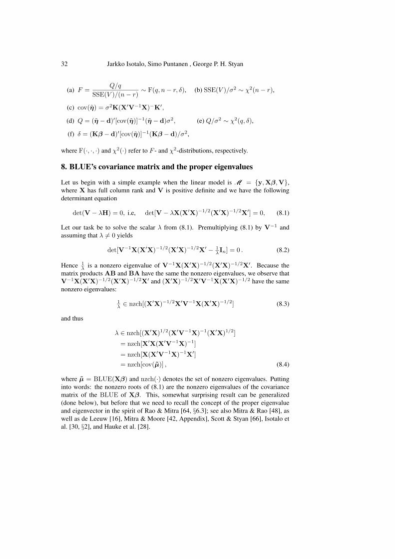
32 Jarkko Isotalo, Simo Puntanen , George P. H. Styan
(a) F =Q/q
SSE(V )/(n− r)∼ F(q, n− r, δ), (b) SSE(V )/σ2 ∼ χ2(n− r),
(c) cov(η) = σ2K(X′V−1X)−K′,
(d) Q = (η − d)′[cov(η)]−1(η − d)σ2, (e) Q/σ2 ∼ χ2(q, δ),
(f) δ = (Kβ − d)′[cov(η)]−1(Kβ − d)/σ2,
where F(·, ·, ·) and χ2(·) refer to F - and χ2-distributions, respectively.
8. BLUE’s covariance matrix and the proper eigenvalues
Let us begin with a simple example when the linear model is M = y,Xβ,V,where X has full column rank and V is positive definite and we have the following
determinant equation
det(V − λH) = 0, i.e, det[V − λX(X′X)−1/2(X′X)−1/2X′] = 0, (8.1)
Let our task be to solve the scalar λ from (8.1). Premultiplying (8.1) by V−1 and
assuming that λ 6= 0 yields
det[V−1X(X′X)−1/2(X′X)−1/2X′ − 1λIn] = 0 . (8.2)
Hence 1λ is a nonzero eigenvalue of V−1X(X′X)−1/2(X′X)−1/2X′. Because the
matrix products AB and BA have the same the nonzero eigenvalues, we observe that
V−1X(X′X)−1/2(X′X)−1/2X′ and (X′X)−1/2X′V−1X(X′X)−1/2 have the same
nonzero eigenvalues:
1λ ∈ nzch[(X′X)−1/2X′V−1X(X′X)−1/2] (8.3)
and thus
λ ∈ nzch[(X′X)1/2(X′V−1X)−1(X′X)1/2]
= nzch[X′X(X′V−1X)−1]
= nzch[X(X′V−1X)−1X′]
= nzch[cov(µ)] , (8.4)
where µ = BLUE(Xβ) and nzch(·) denotes the set of nonzero eigenvalues. Putting
into words: the nonzero roots of (8.1) are the nonzero eigenvalues of the covariance
matrix of the BLUE of Xβ. This, somewhat surprising result can be generalized
(done below), but before that we need to recall the concept of the proper eigenvalue
and eigenvector in the spirit of Rao & Mitra [64, §6.3]; see also Mitra & Rao [48], as
well as de Leeuw [16], Mitra & Moore [42, Appendix], Scott & Styan [66], Isotalo et
al. [30, §2], and Hauke et al. [28].
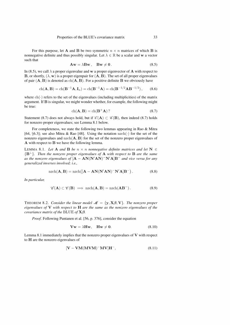
Properties of the BLUE’s covariance matrix 33
For this purpose, let A and B be two symmetric n × n matrices of which B is
nonnegative definite and thus possibly singular. Let λ ∈ R be a scalar and w a vector
such that
Aw = λBw , Bw 6= 0 . (8.5)
In (8.5), we call λ a proper eigenvalue and w a proper eigenvector of A with respect to
B, or shortly, (λ,w) is a proper eigenpair for (A,B). The set of all proper eigenvalues
of pair (A,B) is denoted as ch(A,B). For a positive definite B we obviously have
ch(A,B) = ch(B−1A, In) = ch(B−1A) = ch(B−1/2AB−1/2) , (8.6)
where ch(·) refers to the set of the eigenvalues (including multiplicities) of the matrix
argument. If B is singular, we might wonder whether, for example, the following might
be true:
ch(A,B) = ch(B+A) ? (8.7)
Statement (8.7) does not always hold, but if C (A) ⊂ C (B), then indeed (8.7) holds
for nonzero proper eigenvalues; see Lemma 8.1 below.
For completeness, we state the following two lemmas appearing in Rao & Mitra
[64, §6.3]; see also Mitra & Rao [48]. Using the notation nzch(·) for the set of the
nonzero eigenvalues and nzch(A,B) for the set of the nonzero proper eigenvalues of
A with respect to B we have the following lemma.
LEMMA 8.1. Let A and B be n × n nonnegative definite matrices and let N ∈B⊥. Then the nonzero proper eigenvalues of A with respect to B are the same
as the nonzero eigenvalues of [A − AN(N′AN)−N′A]B− and vice versa for any
generalized inverses involved; i.e.,
nzch(A,B) = nzch([A−AN(N′AN)−N′A]B−
). (8.8)
In particular,
C (A) ⊂ C (B) =⇒ nzch(A,B) = nzch(AB−) . (8.9)
THEOREM 8.2. Consider the linear model M = y,Xβ,V. The nonzero proper
eigenvalues of V with respect to H are the same as the nonzero eigenvalues of the
covariance matrix of the BLUE of Xβ.
Proof. Following Puntanen et al. [56, p. 376], consider the equation
Vw = λHw, Hw 6= 0. (8.10)
Lemma 8.1 immediately implies that the nonzero proper eigenvalues of V with respect
to H are the nonzero eigenvalues of
[V −VM(MVM)−MV]H−, (8.11)
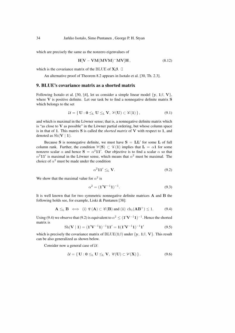
34 Jarkko Isotalo, Simo Puntanen , George P. H. Styan
which are precisely the same as the nonzero eigenvalues of
H[V −VM(MVM)−MV]H , (8.12)
which is the covariance matrix of the BLUE of Xβ.
An alternative proof of Theorem 8.2 appears in Isotalo et al. [30, Th. 2.3].
9. BLUE’s covariance matrix as a shorted matrix
Following Isotalo et al. [30, §4], let us consider a simple linear model y, 1β, V,where V is positive definite. Let our task be to find a nonnegative definite matrix S
which belongs to the set
U = U : 0 ≤L U ≤L V, C (U) ⊂ C (1) , (9.1)
and which is maximal in the Lowner sense; that is, a nonnegative definite matrix which
is “as close to V as possible” in the Lowner partial ordering, but whose column space
is in that of 1. This matrix S is called the shorted matrix of V with respect to 1, and
denoted as Sh(V | 1).Because S is nonnegative definite, we must have S = LL′ for some L of full
column rank. Further, the condition C (S) ⊂ C (1) implies that L = α1 for some
nonzero scalar α and hence S = α211′. Our objective is to find a scalar α so that
α211′ is maximal in the Lowner sense, which means that α2 must be maximal. The
choice of α2 must be made under the condition
α211′ ≤L V. (9.2)
We show that the maximal value for α2 is
α2 = (1′V−11)−1. (9.3)
It is well known that for two symmetric nonnegative definite matrices A and B the
following holds see, for example, Liski & Puntanen [38]:
A ≤L B ⇐⇒ (i) C (A) ⊂ C (B) and (ii) ch1(AB+) ≤ 1. (9.4)
Using (9.4) we observe that (9.2) is equivalent to α2 ≤ (1′V−11)−1. Hence the shorted
matrix is
Sh(V | 1) = (1′V−11)−111′ = 1(1′V−11)−11′ (9.5)
which is precisely the covariance matrix of BLUE(1β) under y, 1β, V. This result
can be also generalized as shown below.
Consider now a general case of U :
U = U : 0 ≤L U ≤L V, C (U) ⊂ C (X) . (9.6)
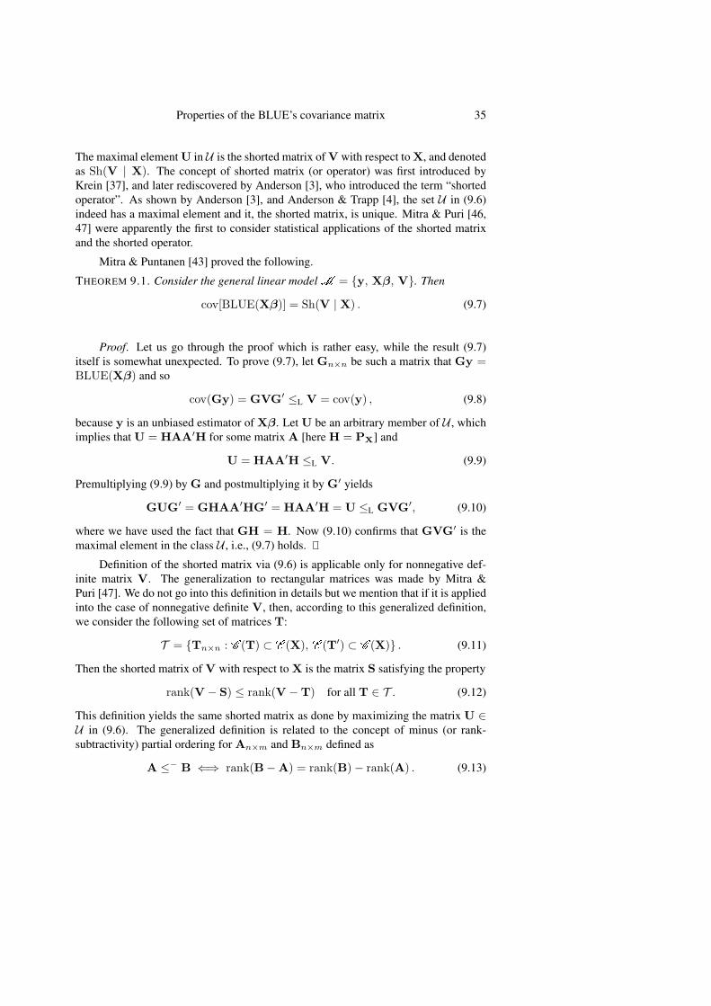
Properties of the BLUE’s covariance matrix 35
The maximal element U in U is the shorted matrix of V with respect to X, and denoted
as Sh(V | X). The concept of shorted matrix (or operator) was first introduced by
Krein [37], and later rediscovered by Anderson [3], who introduced the term “shorted
operator”. As shown by Anderson [3], and Anderson & Trapp [4], the set U in (9.6)
indeed has a maximal element and it, the shorted matrix, is unique. Mitra & Puri [46,
47] were apparently the first to consider statistical applications of the shorted matrix
and the shorted operator.
Mitra & Puntanen [43] proved the following.
THEOREM 9.1. Consider the general linear modelM = y, Xβ, V. Then
cov[BLUE(Xβ)] = Sh(V | X) . (9.7)
Proof. Let us go through the proof which is rather easy, while the result (9.7)
itself is somewhat unexpected. To prove (9.7), let Gn×n be such a matrix that Gy =BLUE(Xβ) and so
cov(Gy) = GVG′ ≤L V = cov(y) , (9.8)
because y is an unbiased estimator of Xβ. Let U be an arbitrary member of U , which
implies that U = HAA′H for some matrix A [here H = PX] and
U = HAA′H ≤L V. (9.9)
Premultiplying (9.9) by G and postmultiplying it by G′ yields
GUG′ = GHAA′HG′ = HAA′H = U ≤L GVG′, (9.10)
where we have used the fact that GH = H. Now (9.10) confirms that GVG′ is the
maximal element in the class U , i.e., (9.7) holds.
Definition of the shorted matrix via (9.6) is applicable only for nonnegative def-
inite matrix V. The generalization to rectangular matrices was made by Mitra &
Puri [47]. We do not go into this definition in details but we mention that if it is applied
into the case of nonnegative definite V, then, according to this generalized definition,
we consider the following set of matrices T:
T = Tn×n : C (T) ⊂ C (X), C (T′) ⊂ C (X) . (9.11)
Then the shorted matrix of V with respect to X is the matrix S satisfying the property
rank(V − S) ≤ rank(V −T) for all T ∈ T . (9.12)
This definition yields the same shorted matrix as done by maximizing the matrix U ∈U in (9.6). The generalized definition is related to the concept of minus (or rank-
subtractivity) partial ordering for An×m and Bn×m defined as
A ≤− B ⇐⇒ rank(B−A) = rank(B)− rank(A) . (9.13)
36 Jarkko Isotalo, Simo Puntanen , George P. H. Styan
For the following lemma, see Mitra et al. [44].
LEMMA 9.2. The following statements are equivalent when considering the linear
model y,Xβ,V with X∼ being a generalized inverse of X.
(a) XX∼V(X∼)′X′ ≤L V,
(b) XX∼y is the BLUE for Xβ,
(c) XX∼V(X∼)′X′ ≤− V,
(d) XX∼V(X∼)′X′ = Sh(V | X).
For a review of shorted matrices and their applications in statistics, see Mitra et
al. [44] and Mitra et al. [41], and for relations of shorted matrices and matrix partial
orderings, see, e.g., Mitra & Prasad [45], Eagambaram et al. [20] and Prasad et al. [52].
10. Best linear unbiased predictor, BLUP
We can extend the modelM = y,Xβ,V by considering a q× 1 random vector y∗,
which is an unobservable random vector containing new future observations. These
new observations are assumed to be generated from
y∗ = X∗β + ε∗ , (10.1)
where X∗ is a known q × p matrix, β ∈ Rp is the same vector of fixed but unknown
parameters as in M , and ε∗ is a q-dimensional random error vector with E(ε∗) = 0.
We will also use the notations µ = Xβ and µ∗ = X∗β. The covariance matrix of y∗
and the cross-covariance matrix between y and y∗ are assumed to be known and thus
we have
E
(y
y∗
)=
(µ
µ∗
)=
(X
X∗
)β , cov
(y
y∗
)=
(V V12
V21 V22
)= Γ , (10.2)
where the (n+ q)× (n+ q) covariance matrix Γ is known. This setup can be denoted
shortly as
M∗ =
(y
y∗
),
(X
X∗
)β,
(V V12
V21 V22
). (10.3)
We are particularly interested in predicting the unobservable y∗ on the basis of the
observable y. While doing this, we look for linear predictors of the type Ay, where
A ∈ Rq×n.
The random vector y∗ is called predictable under M∗ if there exists a matrix A
such that the expected prediction error is zero, i.e., E(y∗ −Ay) = 0 for all β ∈ Rp.Then Ay is a linear unbiased predictor (LUP) of y∗. Such a matrix A ∈ Rq×n exists
if and only if C (X′∗) ⊂ C (X′), that is, X∗β is estimable under M . Thus y∗ is
Properties of the BLUE’s covariance matrix 37
predictable under M∗ if and only if X∗β is estimable. Now a LUP Ay is the best
linear unbiased predictor, BLUP, for y∗, if we have the Lowner ordering
cov(y∗ −Ay) ≤L cov(y∗ −A#y) for all A# : A#X = X∗ . (10.4)
Theorem 10.1 below provides so-called fundamental BLUP equations, see, e.g.,
Christensen [13, p. 294], and Isotalo & Puntanen [32, p. 1015], For the reviews of the
BLUP-properties, see, Robinson [65] and Haslett & Puntanen [27].
THEOREM 10.1. Consider the linear model with new observations defined as M∗ in
(10.3), where C (X′∗) ⊂ C (X′), i.e., y∗ is predictable. Then the linear predictor Ay
is the BLUP for y∗ if and only if A ∈ Rq×n satisfies the equation
A(X : VX⊥) = (X∗ : V21X⊥) . (10.5)
Moreover, the linear predictor By is the BLUP for ε∗ if and only if B ∈ Rq×n satisfies
the equation
B(X : VX⊥) = (0 : V21X⊥) . (10.6)
We will use the following short notations:
y∗ = BLUP(y∗) , µ∗ = BLUE(µ∗) , ε∗ = BLUP(ε∗) . (10.7)
Suppose that the parametric function µ∗ = X∗β is estimable underM∗ which happens
if and only if C (X′∗) ⊂ C (X′) so that
X∗ = LX for some matrix L ∈ Rq×f , µ∗ = X∗β = LXβ = Lµ . (10.8)
Now the BLUP(y∗) underM∗, see, e.g., Isotalo et al. [31, Sec. 4], can be written as
y∗ = µ∗ + ε∗ , (10.9)
and further as
BLUP(y∗) = BLUE(µ∗) + BLUP(ε∗)
= LGy +V21V−(In −G)y
= LGy +V21M(MVM)−My , (10.10)
where G = PX;W− = X(X′W−X)−X′W−, and W ∈ W∗.
What about the covariance matrix of BLUP(y∗)? We observe that the random
vectors µ∗ and ε∗ are uncorrelated and so
cov(y∗) = cov(µ∗) + cov(ε∗) . (10.11)
38 Jarkko Isotalo, Simo Puntanen , George P. H. Styan
Now we have
cov(µ∗) = L cov(µ)L′, cov(ε∗) = V21M(MVM)−MV12 . (10.12)
For calculating the covariance matrix of the prediction error y∗ − y∗, it is conve-
nient to express the prediction error as
y∗ − y∗ = (y∗ −V21V−y) + (V21V
−y − y∗) , (10.13)
see Sengupta & Jammalamadaka [67, p. 292]. In view of (10.10), we get
y∗ − y∗ = (y∗ −V21V−y) + (V21V
− − L)Gy
= (y∗ −V21V−y) +Nµ , (10.14)
where N = V21V−−L. The random vectors y∗−V21V
−y and Nµ are uncorrelated
and hence
cov(y∗ − y∗) = cov(y∗ −V21V−y) + cov(Nµ)
= V22 −V21V−V12 +N cov(µ)N′. (10.15)
The first term Γ22·1 := V22 −V21V−V12 in (10.15) is the Schur complement of V
in
Γ =
(V V12
V21 V22
), (10.16)
and as Sengupta & Jammalamadaka [67, p. 293] point out, Γ22·1 is the covariance
matrix of the prediction error associated with the best linear predictor, BLP, (supposing
that Xβ were known) while the second term represents the increase in the covariance
matrix of the prediction error due to estimation of Xβ.
We may complete our paper by briefly touching the concept of the best linear
predictor, BLP. Notice first that the word “unbiased” is missing in this concept. The
following lemma is essential when dealing with the best linear prediction; see, e.g.,
Puntanen et al. [56, Ch. 9].
LEMMA 10.2.
Let u and v be u- and v-dimensional random vectors, respectively, and let z =(uv
)be a partitioned random vector with covariance matrix
cov(z) = cov
(u
v
)=
(Ωuu Ωuv
Ωvu Ωvv
)= Ω . (10.17)
Then
cov(v − Fu) ≥L cov(v −ΩvuΩ−uuu) for all F ∈ Rv×u, (10.18)
Properties of the BLUE’s covariance matrix 39
and the minimal covariance matrix is
cov(v −ΩvuΩ−uuu) = Ωvv −ΩvuΩ
−uuΩuv = Ωvv·u , (10.19)
the Schur complement of Ωuu in Ω.
A linear predictor Cu + c, where C ∈ Rv×u and c ∈ Rv , is the best linear
predictor, BLP, of the random vector v on the basis of u if it minimizes, in the Lowner
sense, the mean squared error matrix
E[v − (Cu+ c)][v − (Cu+ c)]′ = cov(v −Cu) + ‖µv − (Cµu + c)‖2, (10.20)
where µu = E(u) and µv = E(v). The random vector v = µv + ΣvuΣ−uu(u −
µu) appears to be the BLP of v on the basis of u, and the covariance matrix of the
prediction error v − v is Ωvv·u.
In Lemma 10.2 our attempt is to find a matrix F which minimizes the covariance
matrix of the difference v − Fu. This is strikingly close to the task of finding the
BLUP for y∗, where we are minimizing the covariance matrix of the prediction error
y∗ −Ay. However, the major difference between these two tasks is that in (10.18) we
have no restrictions to F while in (10.4) we assume that AX = X∗.
Acknowledgements
The authors thank the support of so and so project/funding. Part of this article was pre-
sented by Simo Puntanen in The Fourth DAE-BRNS Theme Meeting on Generation and
use of Covariance Matrices in the Applications of Nuclear Data, Manipal University,
Manipal, Karnataka, India, 9–13 December 2017. Thanks go to Professor K. Manju-
natha Prasad and his team for excellent hospitality. Due to the topic of this conference,
it might be appropriate to cite a few words from the Appendix of article [58], published
by Professor C. Radhakrishna Rao in 1971. The title of the Appendix was “The Atom
Bomb and Generalized Inverse”. Below the first and last paragraph of the Appendix
are quoted.
“The author was first led to the definition of a pseudo-inverse (now called
generalized inverse or g-inverse) of a singular matrix in 1945–1955 when
he undertook to carry out multivariate analysis of anthropometric data ob-
tained on families of Hiroshima and Nagasaki to study the effects of radi-
ation due atom bomb explosions, on request from Dr. W.J. Schull of the
University of Michigan. The computation and use of a pseudo-inverse are
given in a statistical report prepared by the author, which is incorporated
in Publication No. 461 of the National Academy of Sciences, U.S.A., by
Neel and Schull (1956), [50]. It may be of interest to the audience to know
the circumstances under which the pseudo-inverse had to be introduced.”
“It is hard to believe that scientist have found in what has been described
as the greatest tragedy a source for providing material and simulation for
research in many directions.”
40 Jarkko Isotalo, Simo Puntanen , George P. H. Styan
REFERENCES
[1] Aitken A.C. (1936). On least squares and linear combination of observations.
Proc. Roy. Soc. Edinburgh Sect. A, 55, 42–48.
[2] Anderson, T.W. (2003). An Introduction to Multivariate Statistical Analysis,
3rd Ed. Wiley, New York.
[3] Anderson W.N. Jr. (1971). Shorted operators. SIAM J. Appl. Math., 20, 520–
525.
[4] Anderson, W.N. Jr. & Trapp G.E. (1975). Shorted operators, II. SIAM J. Appl.
Math., 28, 60–71.
[5] Baksalary J.K. & Kala R. (1981). Linear transformations preserving best linear
unbiased estimators in a general Gauss–Markoff model. Ann. Statist., 9, 913–
916.
[6] Baksalary J.K. & Kala R. (1986). Linear sufficiency with respect to a given
vector of parametric functions. J. Statist. Plann. Inference, 14, 331–338.
[7] Baksalary J.K. & Mathew T. (1990). Rank invariance criterion and its applica-
tion to the unified theory of least squares. Linear Algebra Appl., 127, 393–401.
[8] Baksalary J.K. & Puntanen S. (1989). Weighted-least-squares estimation in
the general Gauss–Markov model. Statistical Data Analysis and Inference.
(Y. Dodge, ed.) Elsevier Science Publishers B.V., Amsterdam, 355–368.
[9] Baksalary J.K. & Puntanen S. (1991). Generalized matrix versions of the
Cauchy–Schwarz and Kantorovich inequalities. Aequationes Mathematicae,
41, 103–110.
[10] Baksalary J.K., Puntanen S. & Styan G.P.H. (1990). A property of the disper-
sion matrix of the best linear unbiased estimator in the general Gauss–Markov
model. Sankhya Ser. A, 52, 279–296.
[11] Bartmann F.C. & Bloomfield P. (1981). Inefficiency and correlation.
Biometrika, 68, 67–71.
[12] Bloomfield P. & Watson G.S. (1975). The inefficiency of least squares.
Biometrika, 62, 121–128.
[13] Christensen R. (2011). Plane Answers to Complex Questions: the Theory of
Linear Models, 4th Ed. Springer, New York.
[14] Chu K.L., Isotalo J., Puntanen S. & Styan G.P.H. (2004). On decomposing the
Watson efficiency of ordinary least squares in a partitioned weakly singular
linear model. Sankhya, 66, 634–651.
Properties of the BLUE’s covariance matrix 41
[15] Chu K.L., Isotalo J., Puntanen S. & Styan G.P.H. (2005). Some further results
concerning the decomposition of the Watson efficiency in partitioned linear
models. Sankhya, 67, 74–89.
[16] de Leeuw J. (1982). Generalized eigenvalue problems with positive semidefi-
nite matrices. Psychometrika, 1, 87–93.
[17] Drury S.W., Liu S., Lu C.-Y., Puntanen S. & Styan G.P.H. (2002). Some com-
ments on several matrix inequalities with applications to canonical correlations:
historical background and recent developments. Sankhya Ser. A, 64, 453–507.
[18] Drygas H. (1970). The Coordinate-Free Approach to Gauss–Markov Estima-
tion. Springer, Berlin.
[19] Drygas H. (1983). Sufficiency and completeness in the general Gauss–Markov
model. Sankhya Ser. A, 45, 88–98.
[20] Eagambaram M., Prasad K.M. & Mohana K.S. (2013). Column space decom-
position and partial order on matrices. Electron. J. Linear Algebra, 26, 795–
815.
[21] Groß J. & Puntanen S. (2000). Estimation under a general partitioned linear
model. Linear Algebra Appl. 321,131–144.
[22] Groß J. & Trenkler G. (1998). On the equality of linear statistics in general
Gauss–Markov Model. Frontiers in Probability and Statistics. (S.P. Mukherjee,
S.K. Basu & B.K. Sinha, eds.) Narosa Publishing House, New Delhi, pp.189–
194. [Proc. of the Second International Triennial Calcutta Symposium on Prob-
ability and Statistics, Calcutta, 30 December 1994 – 2 January 1995.]
[23] Gustafson K. (1972). Antieigenvalue inequalities in operator theory. Inequali-
ties, III (Proc. Third Sympos., Univ. California, Los Angeles, 1969; Dedicated
to the Memory of Theodore S.Motzkin). (O. Shisha, ed.) Academic Press, New
York, pp. 115–119.
[24] Gustafson K. (2006). The trigonometry of matrix statistics. Internat. Statist.
Rev., 74, 187–202.
[25] Gustafson K. (2012). Antieigenvalue Analysis. World Scientific, Singapore.
[26] Haslett S.J., Isotalo J., Liu Y. & Puntanen S. (2014). Equalities between OLSE,
BLUE and BLUP in the linear model. Statist. Papers, 55, 543–561.
[27] Haslett S.J. & Puntanen S. (2017). Best linear unbiased prediction (BLUP).
Wiley StatsRef: Statistics Reference Online.
[28] Hauke J., Markiewicz A. & Puntanen S. (2013). Revisiting the BLUE in a
linear model via proper eigenvectors. Combinatorial Matrix Theory and Gen-
eralized Inverses of Matrices. (R.B. Bapat, S. Kirkland, K. M. Prasad & S.
Puntanen, eds.) Springer, pp. 73–83.
42 Jarkko Isotalo, Simo Puntanen , George P. H. Styan
[29] Isotalo J., Puntanen S. & Styan G.P.H. (2008). A useful matrix decomposi-
tion and its statistical applications in linear regression. Comm. Statist. Theory
Methods, 37, 1436–1457.
[30] Isotalo J., Puntanen S. & Styan G.P.H. (2008). The BLUE’s covariance matrix
revisited: a review. J. Statist. Plann. Inference, 138/9, 2722–2737.
[31] Isotalo J., Markiewicz A. & Puntanen S. (2017). Some properties of linear
prediction sufficiency in the linear model. Proceedings of the LINSTAT-2016
(International Conference on Trends and Perspectives in Linear Statistical In-
ference, Istanbul, Turkey, 22–25 August 2016). (M. Tez & D. von Rosen, eds.)
Springer, in press.
[32] Isotalo J. & Puntanen S. (2006). Linear prediction sufficiency for new obser-
vations in the general Gauss–Markov model. Comm. Statist. Theory Methods,
35, 1011–1023.
[33] Kala R., Markiewicz A. & Puntanen S. (2017). Some further remarks on the
linear sufficiency in the linear model. Applied and Computational Matrix Anal-
ysis: MatTriad, Coimbra, Portugal, September 2015, Selected, Revised Contri-
butions. (N. Bebiano, ed.) Springer Proceedings in Mathematics & Statistics,
vol. 192, 275–294.
[34] Kala R., Puntanen S. & Tian Y. (2017). Some notes on linear sufficiency.
Statist. Papers, 58, 1–17.
[35] Khatri, C.G. (1966). A note on a MANOVA model applied to problems in
growth curves. Ann. Inst. Stat. Math., 18, 75–86.
[36] Knott M. (1975). On the minimum efficiency of least squares. Biometrika, 62,
129–132.
[37] Krein M.G. (1947). The theory of self-adjoint extensions of semi-bounded Her-
mitian transformations and its applications, I, II (in Russian). Rec. Math. [Mat.
Sbornik] N.S., 20(62), 431–495; 21(63), 365–404.
[38] Liski E.P. & Puntanen S. (1989). A further note on a theorem on the difference
of the generalized inverses of two nonnegative definite matrices. Comm. Statist.
Theory Methods, 18, 1747–1751.
[39] Markiewicz A. & Puntanen S. (2015). All about the ⊥ with its applications in
the linear statistical models. Open Mathematics, 13, 33–50.
[40] Marsaglia G. & Styan G.P.H. (1974). Equalities and inequalities for ranks of
matrices. Linear Multilinear Algebra, 2, 269–292.
[41] Mitra S.K., Bhimasankaram P. & Malik S.B. (2010). Matrix Partial Orders,
Shorted Operators and Applications. World Scientific, Singapore.
Properties of the BLUE’s covariance matrix 43
[42] Mitra S.K. & Moore B.J. (1973). Gauss–Markov estimation with an incorrect
dispersion matrix. Sankhya Ser. A, 35, 139–152.
[43] Mitra S.K. & Puntanen S. (1991). The shorted operator statistically interpreted.
Calcutta Statist. Assoc. Bull., 40, 97–102.
[44] Mitra S.K., Puntanen S. & Styan G.P.H. (1995). Shorted matrices and their ap-
plications in linear statistical models: a review. Multivariate Statistics and Ma-
trices in Statistics: Proceedings of the 5th Tartu Conference, Tartu–Puhajarve,
Estonia, 23–28 May 1994. (E.-M. Tiit, T. Kollo & H. Niemi, eds.) New Trends
in Probability and Statistics, vol. 3, VSP, Utrecht, Netherlands & TEV, Vilnius,
Lithuania, pp. 289–311.
[45] Mitra S.K. & Prasad K.M. (1996). The nonunique shorted matrix. Linear Al-
gebra Appl., 237/238, 41–70.
[46] Mitra S.K. & Puri M.L. (1979). Shorted operators and generalized inverses of
matrices. Linear Algebra Appl., 25, 45–56.
[47] Mitra, S.K. & Puri M.L. (1982). Shorted matrices – an extended concept and
some applications. Linear Algebra Appl., 42, 57–79.
[48] Mitra S.K. & Rao C.R. (1968). Simultaneous reduction of a pair of quadratic
forms. Sankhya Ser. A, 30, 313–322.
[49] Mitra S.K. & Rao C.R. (1974). Projections under seminorms and generalized
Moore–Penrose inverses. Linear Algebra and Appl., 9, 155–167.
[50] Neel J.V. & Schull W.J. (1956). The effect of exposure to the atomic bomb
on pregnancy termination in Hiroshima and Nagasaki. National Academy of
Sciences National Research Council, Washington, D.C., Publ. No. 461.
[51] Pecaric J.E., Puntanen S. & Styan G.P.H. (1996). Some further matrix exten-
sions of the Cauchy–Schwarz and Kantorovich inequalities, with some statisti-
cal applications. Linear Algebra Appl., 237/238, 455–477.
[52] Prasad K.M, Mohana K.S. & Sheela Y.S. (2013). Matrix partial orders asso-
ciated with space preorder. Combinatorial Matrix Theory and Generalized In-
verses of Matrices. (R.B. Bapat, S. Kirkland, K.M. Prasad & S. Puntanen, eds.)
Springer, pp. 195–226.
[53] Puntanen S. & Scott A.J. (1996). Some further remarks on the singular linear
model. Linear Algebra Appl., 237/238, 313–327.
[54] Puntanen S. & Styan G.P.H. (1989). The equality of the ordinary least
squares estimator and the best linear unbiased estimator [with comments by O.
Kempthorne & by S.R. Searle and with “Reply” by the authors]. Amer. Statist.,
43, 153–164.
44 Jarkko Isotalo, Simo Puntanen , George P. H. Styan
[55] Puntanen S. & Styan G.P.H. (2005). Schur complements in statistics and prob-
ability. Chapter 6 In The Schur Complement and Its Applications. (F. Zhang,
ed.) Springer, New York, pp. 163–226.
[56] Puntanen S., Styan G.P.H. & Isotalo J. (2011). Matrix Tricks for Linear Statis-
tical Models: Our Personal Top Twenty. Springer, Heidelberg.
[57] Rao C.R. (1967). Least squares theory using an estimated dispersion matrix
and its application to measurement of signals. Proceedings of the Fifth Berkeley
Symposium on Mathematical Statistics and Probability: Berkeley, California,
1965/1966, vol. 1. (L.M. Le Cam & J. Neyman, eds.) University of California
Press, Berkeley, pp. 355–372.
[58] Rao, C.R. (1971). Unified theory of linear estimation. Sankhya Ser. A, 33, 371–
394. [Corrigendum (1972), 34, p. 194 and p. 477.]
[59] Rao C.R. (1973a). Linear Statistical Inference and its Applications, 2nd Ed.
Wiley, New York.
[60] Rao C.R. (1973b). Representations of best linear estimators in the Gauss–
Markoff model with a singular dispersion matrix. J. Multivariate Anal., 3, 276–
292.
[61] Rao C.R. (1974). Projectors, generalized inverses and the BLUE’s. J. R. Stat.
Soc. Ser. B. Stat. Methodol., 36, 442–448.
[62] Rao C.R. (2005). Antieigenvalues and antisingularvalues of a matrix and ap-
plications to problems in statistics. Res. Lett. Inf. Math. Sci., 8, 53–76.
[63] Rao C.R. (2007). Antieigenvalues and antisingularvalues of a matrix and ap-
plications to problems in statistics. Math. Inequal. Appl., 10, 471–489.
[64] Rao C.R. & Mitra S.K. (1971). Generalized Inverse of Matrices and Its Appli-
cations. Wiley, New York.
[65] Robinson G.K. (1991). That BLUP is a good thing: the estimation of random
effects (discussion: pp. 32–51). Stat. Sci., 6, 15–51.
[66] Scott A.J. & Styan G.P.H. (1985). On a separation theorem for generalized
eigenvalues and a problem in the analysis of sample surveys. Linear Algebra
Appl., 70, 209–224.
[67] Sengupta D. & Jammalamadaka S.R. (2003) Linear Models: An Integrated
Approach. World Scientific, River Edge, NJ.
[68] Styan G.P.H. (1985). Schur complements and linear statistical models. Pro-
ceedings of the First International Tampere Seminar on Linear Statistical Mod-
els and their Applications: Tampere, Finland, August–September 1983. (T.
Pukkila & S. Puntanen, eds.) Dept. of Mathematical Sciences/Statistics, Uni-
versity of Tampere, Tampere, Finland, pp. 37–75.
Properties of the BLUE’s covariance matrix 45
[69] Tian Y. & Puntanen S. (2009). On the equivalence of estimations under a gen-
eral linear model and its transformed models. Linear Algebra Appl., 430, 2622–
2641.
[70] Watson G.S. (1955). Serial correlation in regression analysis, I. Biometrika, 42,
327–341.
[71] Zyskind G. (1967). On canonical forms, non-negative covariance matrices and
best and simple least squares linear estimators in linear models. Ann. Math.
Stat., 38, 1092–1109.
[72] Zyskind G. & Martin F.B. (1969). On best linear estimation and general Gauss–
Markov theorem in linear models with arbitrary nonnegative covariance struc-
ture. SIAM J. Appl. Math., 17, 1190–1202. ,
Properties of the BLUE’s covariance matrix
Correction
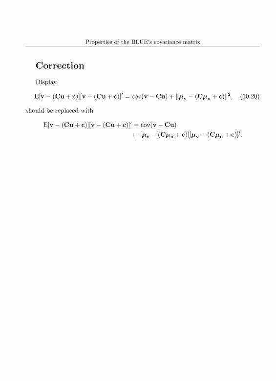
Display
E[v − (Cu + c)][v − (Cu + c)]′ = cov(v −Cu) + ‖µv − (Cµu + c)‖2, (10.20)
should be replaced with
E[v − (Cu + c)][v − (Cu + c)]′ = cov(v −Cu)
+ [µv − (Cµu + c)][µv − (Cµu + c)]′.
26