Sentiments and Economic Activity:

Evidence from U.S. States

Jess Benhabib

New York University

and

Mark M. Spiegel*

Federal Reserve Bank of San Francisco

February 7, 2018

ABSTRACT

We examine whether sentiment influences aggregate demand by studying the relationship between the Michigan Survey expectations concerning national output growth and future economic activity at the state level. We instrument for local sentiments with political outcomes, positing that agents in states with a higher share of congressmen from the political party of the sitting President will be more optimistic. This instrument is strong in the first stage, and our results confirm a positive relationship between sentiments and future state economic activity that is robust to a battery of sensitivity tests.

J.E.L. Classification Number: E20, E32

Keywords: Sentiments, U.S. states, panel estimation, political economy

*Helpful comments were received from Simon Gilchrist, Christian Gillitzer, Oscar Jorda, Atif Mian, Jianjun Miao, Michael Pederson, Morten Ravn, Amir Sufi, Dan Wilson, Tao Zha, the SWUFE International Macro-Finance Conference in Chengdu, China, the Central Bank of Chile Conference on Beliefs, Sentiments and the Macroeconomy, seminar participants at the Federal Reserve Bank of San Francisco, and two anonymous referees. Rebecca Regan and Ben Shapiro provided excellent research assistance. Our views are our own and not necessarily those of the Federal Reserve Board or the Federal Reserve Bank of San Francisco.

1

1. Introduction

There is some evidence of a contemporaneous correlation between measures of consumer

sentiment and economic activity. The headline University of Michigan Index of Consumer

Sentiment (ICS) has been shown to be closely correlated with growth in personal consumption

expenditures over the postwar period [Carroll, et al (1994)]. This observed correlation in the

data can be interpreted in different ways. It is possible that sentiments only reflect knowledge

about current or future economic fundamentals. Some of the empirical literature has therefore

concentrated on testing the restrictions that predict a causal link between sentiment changes and

economic activity. Along these lines, there is also some evidence that sentiment measures

unexplained by economic fundamentals are associated with spending shocks [e.g. Oh and

Waldman (1990), Carroll, et al (1994), Starr (2012)]. However, the contribution of sentiment

shocks “unrelated” to other measures of fundamentals has been found to be only temporary [e.g.

Starr (2012)] and small [e.g. Ludvigson (2004)].1

Nonetheless, some theories suggest that shifts in consumer sentiments, like positive

shocks to expectations concerning future output or future output growth, can indeed be “self-

fulfilling,” and therefore constitute multiple rational expectations equilibria. Indeed these

sentiment-driven, self-fulfilling rational expectations equilibria can arise in various models of

endogenous growth, in models of real business cycles with external effects, in models with

collateral or borrowing constraints, or in search models with aggregate demand externalities, as

well as in OLG models. Stochastic sentiments or sunspots can randomize locally over a

continuum of rational expectations equilibria converging to an indeterminate steady state, or

1 Most of these studies concentrate on the implications of sentiment changes on consumption. Permanent income theories however suggest that agents should spread the impact of improved economic prospects on their consumption over the course of their lifetime. Observed responses over longer time horizons may also be difficult to identify as new shocks emerge and fundamentals respond to changes caused by sentiment shocks.

2

alternatively across distinct multiple steady states.2 Even if the fundamentals-based equilibrium

is unique, information frictions and incomplete markets can give rise to distinct sentiment driven

stochastic rational expectations equilibria.3

Barsky and Sims (2012) distinguish between “animal spirits” shocks and news or

information shocks using a VAR framework.4 They only consider “animal spirits” shocks that

are “erroneous” or irrational, and explicitly exclude sunspot shocks that are self-fulfilling under

rational expectations. They argue that such animal spirits shocks unrelated to fundamentals are

likely to have an immediate but transitory impact on economic activity. Therefore positive

shocks to animal spirits are likely to look like positive aggregate demand shocks in the short run,

but eventually will peter out if they are not followed by real increases in productivity. Using this

assumption as an identification strategy in their VARs, they find that unexplained innovations to

consumer confidence are the result of slowly building news about “apparently permanent”

current and future economic fundamentals, rather than emanating from changes in “animal

spirits” or self-fulfilling expectation shifts that can drive the economy across multiple equilibria

or across multiple steady states.

This interpretation is based on the assumption that sentiment shocks or expectation

shocks that do not reflect news about fundamentals only have temporary effects in equilibrium.

2 See for example Benhabib and Farmer (1999), Benhabib, Schmitt-Grohe and Uribe (2000, 2001), Benhabib and Wang (2013), Howitt and McAfee (1988), and Kaplan and Menzio (2013)]. Self-fulfilling changes in consumer sentiment have also been identified in the literature in a number of alternative ways, as self-fulfilling prophecies [e.g. Azariadis (1981), Farmer (1999), herding [e.g. Blanchard (2016)], and animal spirits [e.g. Keynes (1936) and Akerlof and Shiller (2010)]. Here, unless indicated otherwise, we use changes in sentiments to describe changes in beliefs unrelated to fundamentals. 3 See for example Shell (1977) and Cass and Shell (1983), Maskin and Tirole (1987), Aumann, Peck and Shell (1988), and more recently Angeletos and La’O (2013)], and Benhabib, et al (2015). 4 Also see Levchenko and Pandalai-Nayar (2015) and Fève and Guay (2016), who obtain similar conclusions from alternative structural VAR specifications.

3

However many economic models generate persistent stochastic fluctuations under rational

expectations, driven by sunspot randomizations over multiple equilibria, or by correlated

stochastic equilibria driven by sentiment or expectation shocks. Furthermore, the stochastic

properties of such self-fulfilling equilibria depend, at least in part, on the stochastic processes

driving the sunspots or sentiment shocks, in addition to model-specific internal propagation

mechanisms for such shocks. The sentiment shocks themselves can be driven by general Markov

processes with arbitrary degrees of persistence. Indeed, the fluctuations induced by sentiments

can take the form of randomizations over multiple equilibrium paths around a locally

indeterminate steady state, or alternatively of stochastic fluctuations across multiple steady

states, all under full rational expectations. Depending on the model, these fluctuations can be in

either levels or in growth rates.

In this paper, however, we do not focus on stochastic properties of sentiments

themselves. Instead we focus on the empirical question as to whether consumer sentiments

directly influence output levels over certain time horizons. It is of course quite possible that

sentiment shocks that affect output growth rates are indeed temporary, and our analysis does not

exclude this possibility. What we demonstrate instead is that sentiment or consumer confidence

shocks at the state level do have a measurable impact on state outputs and consumptions,

certainly at one year horizons, and possibly over longer horizons.

We concentrate on U.S. state economic activity as the focus of our analysis. We examine

the responses of overall state economic activity to changes in sentiment about national economic

conditions. Our identification strategy relies on the notion that changes in local sentiment about

national economic prospects are likely to induce local changes in consumption and investment

expenditures. As both consumption and investment expenditures are in play, a focus on

4

aggregate demand and overall economic activity seems useful. Moreover, the output response

provides a guide to the implications of sentiment shocks for optimal stabilization policy.

The use of state data also allows us to condition for aggregate shocks, facilitating the

identification of the direct impact of sentiment changes on economic activity at the state level.

We use Michigan Surveys (2016) questions concerning national economic conditions.

Our base specification uses the question, “Looking ahead, which would you say is more likely --

that in the country as a whole we'll have continuous good times during the next 5 years or so, or

that we will have periods of widespread unemployment or depression, or what?” Our maintained

hypothesis is that states are sufficiently small that attitudes about the local economy will not

distort the response about national economic conditions. Given this assumption, our cross-

sectional treatment should isolate the impact of differences in sentiment across states on future

differences in state economic activity.

While sentiment data is available at the county level, it seems plausible that substantive

leakage is likely to occur across county lines. This is of course a compromise, as leakages across

state lines are also likely to take place, but they are much less likely to be prevalent than those

across county lines.

A potential problem with our specification is that household expectations about future

national economic activity may be positively related to local experiences, raising the prospect of

reverse causality in our empirics. We test for this possibility by examining the impact of past

state growth on current sentiment. We do find evidence of such a relationship in the data, as our

coefficient of interest enters at statistically significant levels in reverse specifications. We

respond to this challenge using instrumental variables estimation. Instrumental variables

5

estimation will also address the likely issue that answers to the Michigan Survey are noisy

measures of consumer sentiment.

We turn to political data as an instrument for local sentiment levels that vary

systematically across states. There is a large literature that demonstrates a positive relationship

between partisanship and economic assessments. A survey respondent that self-identifies as a

member of one of the major political party is more optimistic about the national economic

picture when the sitting national leader is from that same party. In an early paper, Gerber and

Huber (2009) demonstrate that consumption changes following a political election are correlated

with whether or not the election was won by the preferred political party of the respondent. They

interpret this correlation as working through the sentiment channel.

Political partisanship has also been used as an instrument for identifying a connection

between sentiment and consumption.5 Mian, et al (2017) demonstrate that presidential elections

are associated with changes in sentiment about the effectiveness of government policy in line

with political partisanship. However, they find no statistically significant relationship between

changes in the presidential party at the county level in the United States and changes in

consumption.6 In contrast, Gillitzer and Prasad (2016) show in Australian survey data that

higher sentiment -- which is associated with having a member from your political party in office

at the federal level -- is associated with increased future vehicle purchase rates.

The Australian survey data benefits from a direct question about individual political

affiliation. U.S. consumer data, such as that used by Mian, et al (2017) - and also used in this

5 Alternatively, Lagerborg (2017) has used local school shootings as a proxy for sentiment, identifying a negative relationship between sentiment and local unemployment over a one year horizon. 6 Mian, et al (2015) examine the cases of the 2000 and 2008 elections. While in neither case do they find evidence of significant changes in consumption at the county level, they do find a significant correlation between the 2008 election outcome and planned consumption measures consistent with the predictions of a partisanship model.

6

study – require proxies for political partisanship. The Mian, et al study uses county-level data on

voting in presidential elections. Below, we use the share of state congressional representatives

from the same political party as the sitting president. This proxy changes every two years,

yielding more variability in our sample and allowing us to use our full panel sample. This is

desirable because our use of state-level data to mitigate consumption leakages across counties

results in a smaller cross-section than the Mian, et al (2017) county-level study.

We demonstrate below that our proxy is a strong instrument in the first stage of our IV

specification, and that the instrumented measure of consumer sentiment is shown to be positively

and statistically significantly associated with State output growth over the following four

quarters. These results are robust to the inclusion or exclusion of state and time fixed effects, as

well as a variety of sensitivity tests. These include weighting observations by either state size or

the number of respondents, or changes in the sample population, dropping specific time periods,

states with exceptionally high or low incomes, investment levels or populations, or dropping

states identified as outliers based on residual values.7 We also examine robustness to the use of

conventional, rather than heteroskedasticity-corrected standard errors, random instead of fixed

effects, and regional instead of state dummies. The results are also robust to a change in annual

frequencies, and to the inclusion of lagged state and national output growth in our specification.

We also examine alternative sentiment questions. Here our results are more mixed, but

they remain relatively robust for most measures. We also consider the impact of sentiment

7 We do find that our results disappear when we drop the pre-crisis portion of our sample. However, this appears to be the result that we have a relatively small number of non-crisis years available in our sample. As we discuss below, our results are also weaker when we drop the post-crisis years (and strengthen when the crisis years are dropped). It appears that the relationship we identify between sentiment and economic activity broke down during the crisis period.

7

shocks on consumption, in the form of personal consumption expenditures at the state level, and

find that sentiment plays a positive role in the determination of consumption as well.

Finally, we consider longer-horizon sentiment impacts. We repeat our base specification

to investigate the impact of sentiment on state activity and personal consumption expenditures

over 2 and 3 year horizons. Our results for these longer horizons generally remain strong for

both activity and consumption effects, but we find that our longer horizon activity results lose

their significance when we include time dummies and cluster our standard errors by state.

The remainder of this paper is organized into 7 sections. The following section

introduces our data summary statistics. Section 3 discusses our IV methodology. Section 4

describes our base specification results. Section 5 subjects our results to a battery of robustness

tests. Section 6 reports our results for longer horizons. Section 7 concludes.

2. Data

Quarterly sentiment data is available from 2005 through 2016 from the University of

Michigan Surveys of Consumers (2017). Our base gauge of consumer sentiment is the answer to

question BUS5, “Looking ahead, which would you say is more likely -- that in the country as a

whole we'll have continuous good times during the next 5 years or so, or that we will have

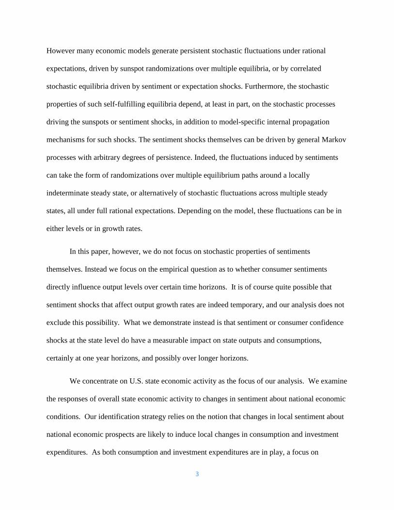
periods of widespread unemployment or depression, or what?” Respondents’ answers are scored

1 through 5, with 1 representing the answer “Good times,” 2 representing “Good with

qualifications,” 3 representing “Pro-Con,” 4 representing “Bad with Qualifications,” 5

representing “Bad Times.” There are also a modest number of responses characterized as

“depends.”. The distribution of responses for the entire sample is shown in Figure 1. It can be

seen that extreme responses of 1 or 5 are most common.

8

Figure 2 displays the relationship between national sentiment and national economic

activity. As in much of the literature, sentiment appears to track current economic activity. For

example, it is clear that sentiment declines sharply in tandem with the onset of the Great

Recession. Still, sentiment does not track activity perfectly. Sentiment reaches its lowest level

Figure 1

Distribution of responses to base sentiment question

Source: Michigan Survey of Consumers, 2004-2013. Histogram of percentages of each answer to survey question BUS5. See text for question.

in 2011, reflecting volatility in financial markets associated with the euro area debt crisis.

Needless to say, while there is a decline in output at this time, it does not match that experienced

during the Great Recession. During that period, sentiment appears to have held up on average

9

while the US economy fell into recession, and then continued to fall after the recession had

ended. The great recession periods is notable, as sentiment appears to track activity much more

closely both before and after the event. Overall though, the raw correlation coefficient between

Figure 2

Average sentiment and national output growth (2004-2015)

Note: Source: Michigan Survey of Consumers, 2004-2015. Sentiment measured by average share of “GOOD” responses (1 or 2) to question BUS5. See text for question. Output growth from current quarter to four quarters in future.

national sentiment and the following year’s national growth in our data is a respectable 0.29.

It is also difficult to draw any causal inferences from this national picture. Changes in

sentiment may be following national economic conditions, rather than leading them. For that

reason, we turn to state activity data for identification. Average consumer sentiment by state

over our sample is shown in appendix Table A1. Reassuringly, there appears to be no apparent

cross-sectional pattern to state sentiment responses, either by income, education, geography, or

10

for the purposes of our IV specification below, political partisanship. In the latter case, note that

our sample period spans years with sitting Presidents from both political parties.8

As our base measure of lagged sentiment, GOOD, we consider the share of a state i at

time t-4 whose respondents’ answers were scored 1 or 2.

We include other variables obtained from the Michigan Surveys to condition on the

characteristics of individual respondents. As our observation is at the state level, these are

measured as state respondent averages, also at time t-4. Our conditioning variables include

income levels by state, INCOME, which is calculated as the average of reported levels of

respondent incomes within a state, EDUC, which is the average of the highest year of education

reported by respondents within a state, and INVEST, which is the share of state respondents who

said that they hold investments. Growth at the state level from period t-4 to t, GGDP, is obtained

from Haver analytics, as is our measure of the national output gap, YGAP.

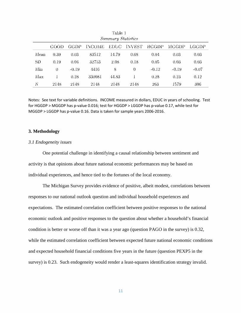
Summary statistics are shown in Table 1. It can be seen that there is a lot of variability in

the data in both growth and sentiment measures, unsurprising since our sample includes the

Great Recession period as well as the boom that preceded it. The final three columns show

average growth rates in our pooled sample for states exhibiting high (more than one standard

deviation above the mean) sentiment levels, HGGDP, neutral (within one standard deviation of

the mean) sentiment levels, MGGDP, and low (more than one standard deviation below the

mean), LGGDP, sentiment levels. As expected, it can be seen that subsequent growth on

average is higher following reports of high sentiment levels, and lower for states where low

levels of sentiment on average are reported. However, t-tests for differences in these populations

are not statistically significant.

8 For our sample period, respondents in the state of Virginia are most optimistic about future national economic activity on average, while those from New Mexico proved the most pessimistic on average.

11

Notes: See text for variable definitions. INCOME measured in dollars, EDUC in years of schooling. Test for HGGDP > MGGDP has p-value 0.016; test for HGGDP > LGGDP has p-value 0.17, while test for MGGDP > LGGDP has p-value 0.16. Data is taken for sample years 2006-2016.

3. Methodology

3.1 Endogeneity issues

One potential challenge in identifying a causal relationship between sentiment and

activity is that opinions about future national economic performances may be based on

individual experiences, and hence tied to the fortunes of the local economy.

The Michigan Survey provides evidence of positive, albeit modest, correlations between

responses to our national outlook question and individual household experiences and

expectations. The estimated correlation coefficient between positive responses to the national

economic outlook and positive responses to the question about whether a household’s financial

condition is better or worse off than it was a year ago (question PAGO in the survey) is 0.32,

while the estimated correlation coefficient between expected future national economic conditions

and expected household financial conditions five years in the future (question PEXP5 in the

survey) is 0.23. Such endogeneity would render a least-squares identification strategy invalid.

12

To test if this is the case using our panel data, we examine the relationship between

current state economic growth and current sentiment levels. Our reverse specification is a

conventional panel estimator

{ } { }4, 4 4

i

t tit it t i t itGOOD y X YGAPα β γ δ ε η− − −= + ∆ + + + + + (1)

where itGOOD represents the share of respondents with positive sentiment responses in state i in period

4t − , 4,

i

t ty

−∆ represents income growth in state i from period 4t − to the present, 4itX − is a vector of

controls linked to state growth via a set of nuisance parameters γ , { }iδ and { }tε are respectively state

and time-specific fixed effects, and itη is a is a residual, assumed to be well behaved. Our coefficient of

interest is β , the partial-correlation between sentiment and subsequent state income growth. We use

three covariates in 4itX − to control for other determinants of state growth available from the respondent

survey, including, INCOME, EDUC, and INVEST, all measured at time t-4 and described above.

We consider two alternative methods for conditioning for prevailing economic

conditions. First, we include the start-of-period output gap, 4tYGAP− . Alternatively, we include

yearly time dummies, { }tε . Quarterly time dummies are included below in our IV robustness

checks. We run this specification using ordinary least squares.

It is also quite possible that our data may exhibit heteroscedasticity and correlations

within and across state groups. We therefore use heteroscedasticity-corrected standard errors

throughout, and allow for cross-sectional or state-specific dependence. For cross-sectional

dependence, which is likely across states in our panel, we use Driscoll-Kraay (1998) estimators.

13

Hoechle (2007) demonstrates that Driscoll-Kraay standard errors are well-calibrated when cross-

sectional dependence is present. For state-specific dependence, we include state dummies and

cluster by state.

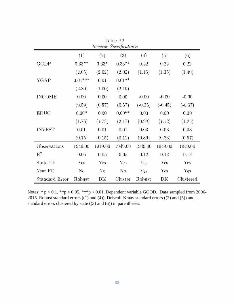
Our results are shown in the appendix of this paper (Table A2). The data do appear to

indicate that sentiment is associated with local activity, although statistical significance is lost

when time dummies are substituted for the national output gap. Overall, however, there does

indeed seem to be a risk of reverse causality.9

3.2 Base IV specification

We address this potential issue through instrumental variables (IV). We follow the

literature in using political data to instrument for differences in sentiment levels by state. Our

posited relationship is that survey respondents will be more optimistic about national economic

prospects if the sitting president is from his or her political party.

Sentiment has been shown in the literature to correspond to economic activity, as in

Gerber and Huber (2009), who identify a positive relationship between partisanship and

economic activity, as consumption changes following a political election are correlated with

whether or not the election was won by the preferred political party of the respondent.

We expect that the primary channel through which partisanship can affect economic

activity is through changes in sentiment. To proxy for political partisanship at the state level, we

use the share of state congressional representatives from the same political party as the sitting

9 As a robustness check, we substituted current quarterly state growth for the previous year’s growth. Our results again indicated the presence of reverse causality, providing further motivation for our base 2SLS specification. These results were provided by the referees and are available from the authors upon request.

14

president, which we term CONGPRES. Our proxy value changes every two years, with each

congressional election.

Our instrument would be invalid if the political situation directly affected underlying

economic fundamentals. For example, it is possible that states with a higher number of

congressional representatives from the same political party as the sitting president will be

favored in political outcomes in a manner that directly supports local economic conditions, such

as decisions about military base closures.

Mian, et al (2017) provide two pieces of evidence against this possibility. First, they look

at income growth in U.S. counties before and after Presidential elections. They find no evidence

that Presidential elections are systematically related to changes in county growth in a manner

associated with local political leanings. Second, they also find no relationship between election

outcomes and changes in government transfers to localities.

We provide additional evidence against this potential problem below, by adding taxes

and transfers from the federal government to our base specification. Our demonstrated

relationship between sentiment and economic activity is robust to conditioning for federal

government taxes and economic transfers.

Our base specification is a conventional two-stage least squares panel estimator. Our first

stage specification for the instrumented share of respondents with positive sentiment responses in state

i in period 4t − satisfies

{ } { }, 4 , 4 4i t i t it i t itGOOD CONGPRES Xφ ξ γ δ ε ν− − −= + + + + + (2)

where 4itGOOD − represents the instrumented share of respondents with positive sentiment responses in

state i in period 4t − , φ represents a constant term, , 4i tCONGPRES − represents the share of state

members of Congress that are in the same party as the sitting President, , 4i tX − is a vector of

15

controls linked to state growth, { }iδ and { }tε are respectively state and time-specific fixed effects, and

,i tν is a is a residual, assumed to be well behaved. We use three covariates in , 4i tX − to control for

other determinants of state growth available from the respondent survey, including, INCOME, EDUC,

and INVEST, defined above.

Our second stage specification is then estimated as:

{ } { }4,

, 4 , 4 4 ,i

t ti t i t t i t i ty GOOD X YGAPα β γ δ ε η

−− − −∆ = + + + + + + (3)

where previously-defined terms are the same as above, 4,

i

t ty

−∆ represents income growth in state i

from period 4t − to the present, 4tYGAP− represents the national output gap prevailing at time 4t −

, and ,i tη is a is a residual, again assumed to be well behaved. Our coefficient of interest isβ , the

partial-correlation between instrumented sentiment and subsequent state income growth. Our lags imply

that our base sample is quarterly from 2006-2016. Our identifying restriction for

, 4i tCONGPRES − in equation (2) is that this variable is uncorrelated with our second stage error

term, ,i tη , as well as the other regressors.10

While our samples are primarily at quarterly frequency, our instrument, , 4i tCONGPRES −

only can change biennially, during Congressional elections, as the data is organized as the share

of members from a given Congress from each party. As such, our sample may have less truly

independent observations than indicated and may exhibit serial correlation. In addition to

10 This assumption is not directly testable. In models where sentiment or sunspot equilibria give rise to economic fluctuations, it is possible to replace the sentiment or sunspot shocks with current or future expected shocks to technology or preferences in order to account for these fluctuations. If it is assumed that sunspot or sentiment shocks have temporary effects while shocks to technology or preferences have permanent effects, then they can be identified as in Barsky and Sims (2012). However in many models sunspot or sentiment shocks can be permanent, as we point out in the introduction.

16

clustering our standard errors by state, in our robustness checks below we examine a smaller

sample with biennial frequency, i.e. with one observation for each state Congressional election

outcome. Our qualitative results are robust to this alternative specification.

For those specifications that include a comprehensive set of both time and state-specific

fixed effects, our specification can be interpreted as a difference-in-differences estimator of the

impact of changes in the share of agents within a state holding positive sentiment about future

national economic prospects or not.

4. Base specification results

We first examine the first stage of our IV specification to demonstrate that we have a

strong instrument. We include our base specification conditioning variables as well. Our panel

results are shown in Table 2. As above, we consider six variations: Models 1 through 3 include

the lagged output gap, while models 4 through 6 include annual time dummies. Models 1 and 4

use robust standard errors, models 2 and 5 use the Driscoll-Kraay estimators, and models 4 and 6

allow for clustered standard errors by state. We include state fixed effects throughout.

Our variable of interest, CONGPRES, consistently enters significantly with its expected

positive sign at a 1% confidence level. Our point estimate for this variable is also largely

invariant to perturbations in our specification. We therefore conclude that we have a strong

instrument and proceed with our IV estimation using a two-stage least squares approach.

The second stage results are shown in Table 3. It can be seen that our variable of interest,

GOOD, enters significantly positively. The instrumented coefficient point estimate in our IV

specification is large. With the income gap included, it comes in at 0.19 and with state fixed

effects included it comes in at 0.13.

17

Notes: * p < 0.1, **p < 0.05, ***p < 0.01. Dependent variable is GOOD. OLS estimation with T-statistics in parentheses. Models 1 and 4 use robust standard errors, models 2 and 5 use the Driscoll-Kraay estimators, and models 4 and 6 allow for clustered standard errors by state. Data is taken for sample years 2004-2015.

Overall, the data support a non-trivial sentiment channel for differences in economic

growth across US states. Indeed, if anything, these point estimates appear to be too high. Under

our Model 1 sample, a one standard deviation increase in sentiment would be associated with an

3.6 percentage point increase in state output growth in Models 1 through 3, and a 2.5 percentage

point increase in Models 4 through 6. However, the 95% confidence intervals for these

18

Notes: * p < 0.1, **p < 0.05, ***p < 0.01. IV estimation with CONGPRES as instrument for GOOD. T-statistics in parentheses. Models 1 and 4 use robust standard errors, models 2 and 5 use the Driscoll-Kraay estimators, and models 4 and 6 allow for clustered standard errors by state. Data is taken from sample years 2006-2016.

coefficients allow a one standard deviation increase in sentiment to be associated with an

increase in state output of as low as 1.1 percentage points, a much more plausible figure, for our

base specification with robust standard errors and the income gap included (Models 1-3), and as

low as 75 basis points with robust standard errors and state fixed effects included (Models 4-6).

19

All of the specifications are statistically significant, at a 1% confidence level using White

heteroscedasticity-robust standard errors, at a 1% confidence level, using Driscoll-Kraay

standard errors, and at a 5% confidence level with standard errors clustered by states using the

output gap and at a 10% confidence level with clustered standard errors with time dummies

instead of the output gap.

The performances of the conditioning variables are mixed. Only the INCOME variable

enters with statistical significance, and then only in our output gap specifications (Models 1

through 3).

Finally, we formally consider the strength of our instruments using the Angrist-Pischke

F-test. The statistic and p-values, shown in Table 3, consistently indicate that our instruments

are strong at statistically significant levels.11

5. Sensitivity analysis

In this section, we demonstrate that our base results, that state sentiments about national

economic prospects have a direct impact on future state output, are quite robust. We first

demonstrate that our base specifications results are largely robust to a wide variety of sample

perturbations (Table 4).

For each sample perturbation, we report the point estimate and standard error for the

coefficient of interest, GOOD, for the six Models in our base specification in Table 3. It can be

seen that the variable of interest is robust to a large majority, but not all permutations. First, we

drop the financial crisis period, which we interpret as spanning from 2007Q4 to 2009Q2. It can

11 We also tested for strong instruments for our specifications at annual and biennial frequencies below. These also indicated strong instruments, and are available on request from the authors.

20

Notes: * p < 0.1, **p < 0.05, ***p < 0.01. IV estimation with CONGPRES as instrument for GOOD. Coefficient estimates are for GOOD sentiment values. T-statistics in parentheses. Models 1 and 4 use robust standard errors, models 2 and 5 use the Driscoll-Kraay estimators, and models 4 and 6 allow for clustered standard errors by state. Data is taken from years 2006-2016.

be seen that our results get stronger with the removal of the crisis period, as we experience

increases in point estimates and significance for all specifications.12 The increased significance

when the crisis period is dropped reassuringly indicates that the crisis does not drive our results.

12 We also tried dropping the first and last 8 quarters of our sample period, but experienced more sensitivity as the crisis period has a larger share is these sub-samples. Our GOOD variable drops out with the early sub-sample omitted. The results are more robust with final 8 quarters dropped, entering at a 5% confidence level for all

21

We next drop observations from “high” (more than one standard deviation above the

mean) and “low” (more than one standard deviation below the mean) average state income

levels. We do the same for high and low shares of households with investments, and states with

large and small GDPs. Finally, we drop outlier observations, measured as those with residuals

more than two and a half standard deviations above or below zero in our base specification.

Our base specification results are robust to dropping high or low incomes, high and low

investments, and large GDP states for all specifications. However, we do observe some

sensitivity to either dropping small GDP or outlier observations. Our results for both sample

perturbations remain significant at least at a 10% level with White heteroscedasticity standard

errors for our base specification with the output gap included, but both alternative samples drop

out with Driscoll-Kraay standard errors and only our drop outliers alternative sample is

significant with standard errors clustered by state.

Table 5 considers the robustness of our results to changes in estimation methodology and

specification. First, given our sample sensitivity to dropping small GDP states, one might be

concerned that averages of sentiment responses from larger states might be more informative, as

these are taken from a larger sample of individual responses. We respond with two types of

weighted least squares estimators, weighting by both state GDP and the number of Michigan

Surveys respondents in the state for that time period. The results for the six specifications with

these weighting schemes for the sample are in the first two rows of Table 5.

Weighting in either manner leaves our coefficient estimate for the variable of interest

significant for all model specifications, with the majority entering at least a 5% confidence level.

output gap specifications, but only at a 10% confidence level for the White and Driscoll-Kraay specifications with time dummies, and narrowly misses significance at a 10% level with standard errors clustered by state. These results are available from the authors on request.

22

Notes: * p < 0.1, **p < 0.05, ***p < 0.01. IV estimation with CONGPRES as instrument for GOOD. Coefficient estimates for GOOD. T-statistics in parentheses. Taxes and transfers include growth in ratio of transfers from the federal government and state Federal income taxes paid. Quarterly data except where indicated. 2148 quarterly obs; 588 annual obs; 539 Taxes and transfers. Robust standard errors (1) and (4), DK (2) and (5), clustered (3) and (6). Data 2006-2016, except Biennial (even years in 2006-2016), and annual and 1 year lagged 2005-2016.

23

Moreover, the change does not qualitatively change our point estimate for output gap

specifications. It falls modestly when weighted by state GDP and marginally rises when

weighted by the n umber of survey responses. We observe larger point estimate declines using

time dummies point estimates respectively. These lower point estimates seem more plausible, as

a one standard deviation increase in the GOOD variable is predicted here to result in 2.1 and 1.9

percentage point increases in state GDP growth respectively.

We also consider conventional, rather than robust standard errors, random, rather than

fixed effects, quarterly, instead of annual, time dummies, and regional dummies instead of state

fixed effects. All specifications continue to enter at standard confidence levels.

We next consider annual, rather than quarterly data. Our annual data is available a year

earlier, and so our sample spans from 2005-2016 and has 588 observations. Our coefficient

estimates for the annual frequency are almost identical to those we obtain with quarterly data,

and our variable of interest remains statistically significant for all specifications.

The use of annual data allows for conditioning on lagged GDP for our base sample

sample period.13 We consider the inclusion of lagged state GDP, lagged US GDP, and both

variables. All specifications enter with qualitatively similar values on our GOOD variable of

interest, and remain statistically significant. The coefficient point estimates are modestly

smaller, but still indicative of a substantive impact of positive sentiment on output. Given a one

13 As a robustness check, we also restricted the annual frequency sample to begin in 2005 instead of 2004, to match the period observed our base sample, running from 2006 through 2016. Our results were robust to the sample change, but the coefficient estimates were notably smaller with lagged state output growth included and just missed statistical significance at 10% confidence levels with heteroscedasticity-consistent standard errors. Still, they were significant with the more general clustering specifications. These results are available from the authors on request.

24

standard deviation increase in our GOOD variable, our point estimate for our base specification

indicates a 2.3 percentage point increase in state output growth.14

As discussed in the introduction, we also consider a biennial frequency sample as a

robustness check, which matches the rest of our data to the biennial frequency of electoral

changes in our instrument. Our results universally demonstrate a positive and statistically

significant relationship between our instrumented sentiment measure and state economic activity.

Moreover, our coefficient point estimates are very close to those obtained in our quarterly base

sample, about 0.22 with the output gap included, vs. 0.19 in our base specification.

We also report our results with ordinary least squares estimation. Our estimated

coefficients for sentiment under OLS are positive and statistically significant with the exception

of standard errors clustered by state. However, our point estimates are smaller than those we

obtain using our IV approach. This may be surprising, as we would expect the bias in our OLS

estimates to be positive due to potential positive reverse causality as we identify in our reverse

regressions. Nevertheless, such an outcome is possible if state sentiment is measured with error,

leading to attenuation bias in our OLS estimation that is corrected by our IV approach.

Finally, as we discuss above, our instrument may be rendered invalid if the political

situation directly affects underlying economic fundamentals. In particular, if states with a higher

number of congressional representatives from the same political party as the sitting president are

14 We also added lagged state GDP at a quarterly frequency, but we lose a year of data, leaving our time spanning 2007-2016. Our estimated coefficient for our variable of interest, GOOD, is positive but loses its significance. However, we also ran the specification under our original sample by linearly interpolating our 2005 annual state output data. Using this sample, the statistical significance for the variable of interest is restored. This alternative sample was provided to the referees and is available on request from the authors.

25

favored in political outcomes that support local economic conditions. We therefore also

condition for federal taxes and growth in transfers in Table 5.15

It can be seen that our results are qualitatively the same with these variables included, as

our point estimates are roughly the same and enter significantly for all specifications. Given this

evidence, we proceed under the assumption that the sentiment channel is the only channel

through which the political characteristics of a state influence its economic activity, rendering

our IV specification valid.

Table 6 considers several alternative sentiment measures to the Michigan Surveys as well

as the impact of sentiment on consumption. Among the alternative sentiment measures, we first

we consider negative responses to the question about future national economic conditions, i.e.

those that answered response “5” to the question above. We term this variable “BAD5”.

Second, we consider the share of respondents in state i at time t that answered the question above

that national economic conditions over the next five years would be “good,” without

qualifications, i.e. with responses that were coded “1” to the question above. We term this

variable “GOOD1.” We also consider responses to question BAGO (109) which asks whether

business conditions are better or worse than the previous year, which we term “BETTER1”.

Finally, we use the sentiment measure studied by Mian, et al (2017) on the quality of government

performance, which we term “GOVT.” We measure this variable as the share of respondents

who answered “1,” indicating that they thought that the government was doing a “good job” in

its economic policy.

15 Taxes are measured as the ratio of state Federal income taxes paid to state income. We measure transfer growth as the growth in transfers from the federal government relative to the previous year. These are introduced as separate variables in our regressions.

26

Notes: * p < 0.1, **p < 0.05, ***p < 0.01. IV estimation with CONGPRES as instrument for indicated sentiment variable. Coefficient estimates for alternative sentiment variables. See text for definitions. Last row reports IV results for consumption, measured by PCE, with GOOD variable as sentiment. GOOD1, BAD5, Better1, GOVT had 2148 observations; PCE is annual data and had 539 Observations. Robust standard errors ((1) and (4)), Driscoll-Kraay standard errors ((2) and (5)) and standard errors clustered by state ((3) and (6)) in parentheses. Data is taken from years 2006-2016 for everything but PCE which is taken from 2005-2015.

Our results for these alternative sentiment measures continue to enter with their expected

signs, but their performances in terms of statistical significance is uneven. Our results for

negative sentiment responses, “BAD5,” universally enters negatively at statistically significant

levels. Our point estimates for this variable indicate a comparable response to what we saw for

our positive sentiment measure. Given the standard error for this variable in our sample of 0.19,

our point estimate of, for example, our base specification with the income gap included and

robust standard errors (Model 1) implies that a one standard deviation increase in the share of

negative sentiment is associated with a 2.7% percentage point decrease in state output growth.

27

Our coefficient estimates for the GOOD1 variable are larger than those in our base

specification above (which is unsurprising as it is on average a more positive response), and are

universally statistically significant at standard confidence level for all of our specifications.

Our results are not as strong for shorter forecast horizons, as the impact of those with

higher expectations concerning business conditions a year from now, BETTER1, consistently

obtains a positive coefficient estimate, but is statistically insignificant for our output gap

specifications, and is also insignificant for the clustered regression with time dummies included.

We obtain stronger results for the specifications where sentiment is measured in terms of

attitudes about the government’s performance, GOVT. These enter significantly for all of the

specifications except Model 6, which clusters and includes time dummies. In that specification,

the variable of interest just barely misses a 10% confidence level of statistical significance.

All of the alternative measures considered enter with their expected signs in all of our

specifications. Not all of these are statistically significant for our sentiment variable of interest.

Overall, while we acknowledge some sensitivity to the sentiment measure used, our results

continue to indicate a positive (negative) impact on state output with higher (lower) measures of

sentiment about future economic activity used.

Finally, a number of papers in the literature [e.g. Gillitzer and Prasad (2016)], examine

the implications of sentiment shocks for consumption, rather than income. These need not go

together, as positive responses in income to sentiment shocks may more reflect movements in

local investment, rather than consumption. We therefore look at the impact of sentiment shocks

on consumption, as measured by movements in personal consumption expenditures. Data for

this variable is available by state only at an annual frequency.

28

Our results are also shown in Table 6. It can be seen that we find a statistically

significant and positive response by state in consumption to sentiment differences as well.

Moreover, the point estimates for our specifications appear to indicate responses of a plausible

and economically significant magnitude, as a one standard deviation increase in GOOD is

predicted to result in a 2.3 percentage point increase in PCE consumption.

6. Impact on activity over longer horizons

Finally, we consider the impact of sentiment over longer horizons. We redo our base

specifications with a two-year lag for sentiment. Our dependent variable is now , 2it tGGDP + , the

average annual state growth from period t through period t+2.

Our results over two and three-year horizons are shown in Table 7. Our specifications for

our base sentiment measure, GOOD, are significant at standard confidence levels for all methods

with the output gap included (models 1 through 3). The coefficient point estimates are a little

smaller, as would be expected over a longer horizon, but still indicate a substantive impact on

state growth from changes in sentiment.16

The results are more mixed for growth over a two year horizon with time fixed effects

included. The coefficient point estimates are smaller, but still indicate a notable impact on

growth. However, while we obtain significant coefficient estimates with robust standard errors,

our results over a two-year horizon are weaker using either Driscoll-Kraay or clustered standard

errors. As above, we have some reservations about our standard error estimates for these

clustered specifications because our panel is small in the time dimension. Our point estimates

16 Another potential reason is that our longer horizons necessitate truncating our sample, to 2007-2016 for a 2-year horizon, and 2008-2016 for a three year. As we discussed earlier, the significance of our results proved sensitive to dropping the pre-crisis periods, which longer horizons partially require.

29

Note: * p < 0.1, **p < 0.05, ***p < 0.01. IV estimation for state GDP and state PCE growth over 2 and 3 years, with CONGPRES as instrument for GOOD variable. Coefficients shown for GOOD variable. T-statistics in parentheses. Models 1 and 4 use robust standard errors, models 2 and 5 use the Driscoll-Kraay estimators, and models 4 and 6 allow for clustered standard errors by state. For 2 year PCE we are sampling from 2006-2015 data.

suggest that under our sample a one standard deviation increase in sentiment is associated with

an 1.6 percentage point increase in average state growth over the next two years for the

specifications with the income gap included (Models 1 through 3), and even smaller effects with

state fixed effects. However, a 95% confidence interval would include values similar to our

point estimates for the one year horizon.

The point estimates for average annual growth are even smaller over a three year horizon,

as might be expected. Our point estimates suggest that a one standard deviation increase in

sentiment is associated with a still-substantial 0.9 percentage point increase in average state

30

growth over the next two years for the specifications with the income gap included (Models 1

through 3), and even smaller effects with state fixed effects included. Again, a 95% confidence

interval includes values similar to our point estimates for the one year horizon. Moreover, it is

important to remember that as the impact period increases in length, the probability that further

unmeasured sentiment shocks took place increases, which adds noise to our analysis.

Our estimates over the 3-year horizon for state growth appear to be weaker, as our point

estimates fall, for example to 0.05 in the case of output gap specifications (Models 1 through 3),

and we only obtain statistically significant coefficient estimates at standard confidence levels

under robust standard error estimation. Our coefficient estimates for models 1 through 3 suggest

that a one standard deviation increase in sentiment results in a 1.0 percentage point increase in

average annual output growth over a three year horizon.

Our results suggest a more modest, but still positive impact of sentiment shocks over

these longer term horizons. Still, our weaker results over these longer–term indicate that the

robust positive impact of state sentiment shocks on output growth that we find in the data for a

one year horizon may be temporary.

We next turn to longer-term impacts on PCE consumption by state, which is only

available at an annual frequency. Our results for two and three year horizons are shown in rows

three and four of Table 7. It can be seen that our point estimates are somewhat lower, but all of

our specifications over both horizons are statistically significant at standard confidence levels.

Overall, our results also confirm a longer-term relationship between sentiment and future

consumption at the state level is persistent. We also obtained positive, but weaker, estimates of

the implications of sentiment shocks for state economic activity.

31

7. Conclusion

We revisit the relationship between consumer sentiment and economic activity. Our

identification strategy is based on using the cross-sectional information in state data. We

examine individual responses to survey questions about long-term prospects for the national

economy. If sentiment drives activity, states in which agents hold more optimistic outlooks

about national economic prospects should undertake higher levels of economic activity:

Sentiments about national economic prospects can thereby affect output at the state level.

A potential problem with our strategy is that it is possible that agents’ responses to

questions about future national economic conditions may reflect local conditions. Our reverse

regression results suggest that reverse causality along these lines may indeed be an issue,

although formal Hausman tests do not indicate endogeneity at statistically significant levels. To

address this potential problem, we turn to IV estimation, based on a predicted relationship

between political partisanship and economic sentiment concerning national economic prospects.

Our results demonstrate a strong first stage relationship between our instrument and our

sentiment measure. Our instrumented sentiment measure confirms a statistically significant

relationship between state sentiment about national economic prospects and next year’s state

economic activity under a variety of specifications. Our point estimate under our base

specification indicates that a one standard deviation increase in sentiment is associated with

additional 49 basis points of growth in the following year. This result is robust to a wide variety

of robustness tests, including sample perturbations, changes in estimation methods, and the use

of alternative sentiment measures. Moreover, we find a significant and robust relationship at

annual frequency between state sentiment and next year’s PCE consumption at the state level.

32

We also consider the impact of sentiment over two and three year horizons. Our results

over these longer horizons are modestly weaker for state output, always entering positively but

not always at statistically significant levels, particularly at the longer three year horizon. Our

results for longer horizons with state PCE consumption are stronger. All of specifications enter

positive at statistically significant levels, regardless of model or estimation method. Still, our

point estimates diminish with horizon, indicating that our data indicate a persistent positive

relationship, but not necessarily a permanent one.

Our overall results therefore support the notion of a positive empirical relationship

between sentiments and future economic activity, as well as future consumption expenditures.

We find weaker impacts at longer horizons for activity, but robust evidence of measurable

impacts on consumption.

Still, it is possible that new sentiment shocks that occur late under the longer horizons

add noise to our sample and preclude finding statistically significance. Therefore, we remain

hesitant to reject the possibility of significant sentiment effects on output at longer horizons. Our

quarterly sample is by necessity small in the time dimension, and with longer samples we may

obtain stronger results over time.

33

References

Akerlof, George A. and Robert J. Shiller, (2010), Animal Spirits: How Human Psychology Drives the Economy, and Why It Matters ..., Princeton University Press.

Angeletos, George-Marios and Jennifer La’O, (2013). Sentiments, Econometrica, 81, 739-779.

Azariadis, Costas, (1981), “Self-Fulfilling Prophecies,” Journal of Economic Theory, 25, 380-396.

Barsky, Robert B. and Eric R. Sims, (2012), “Information, Animal Spirits, and the Meaning of Innovations in Consumer Confidence,” American Economic Review, 102(4), 1343-77.

Benhabib, Jess and Roberto Perli (1994), "Uniqueness and Indeterminacy: On the Dynamics of Endogenous Growth," Journal of Economic Theory, 63, 113-142.

Benhabib, Jess, and Roger Farmer, (1999), “Indeterminacy and Sunspots in Macroeconomics,” in Handbook of Macroeconomics, Vol. 1, J. Taylor and M. Woodford, eds., Amsterdam: North Holland/Elsevier, 387-448.

Benhabib, Jess, Stephanie Schmitt-Grohe and Martin Uribe (2001), “The Perils of Taylor Rules,” Journal of Economic Theory, Vol. 96, Jan 2001, 40-69.

Benhabib, Jess, Pengfei Wang, and Yi Wen, (2015), “Sentiments and Aggregate Demand Fluctuations,” Econometrica, 83(2), 549-585.

Blanchard, Olivier, (2016), “The Price of Oil, China, and Stock Market Herding,” Realtime Economic Issues Watch, Peterson Institute for International Economics, January 17, http://blogs.piie.com/realtime/?p=5341.

Cameron, Colin A., and Pravin K. Trivedi, (2005), Microeconometrics, Cambridge University Press, New York.

Carroll, Christopher D., Jeffrey Fuhrer, and David W. Wilcox, (1994), “Does Consumer Sentiment Forecast Household Spending? If So, Why?,” American Economic Review, 84(5), 1397-1408.

Cass, David and Karl Shell, (1983), “Do Sunspots Matter?,” Journal of Political Economy, 91(2), 193-227.

Farmer, Roger, (1999), The Macroeconomics of Self-Fulfilling Prophecies, MIT Press, Boston.

Fève, Patrick, and Alain Guay, (2016), “Sentiments in SVARs,” mimeo, May.

Gerber, Alan S., and Gregory A. Huber, (2009), “Partisanship and Economic Behavior: Do Partisan Differences in Economic Forecasts Predict Real Economic Behavior?,” American Political Science Review, 103(3), 407-426.

34

Gillitzer, Christian, and Nalini Prasad, (2016), “The Effect of Consumer Sentiment on Consumption: Cross-Sectional Evidence from Elections,” Reserve Bank of Australia Working Paper RDP 2016-10, November.

Hoechle, Daniel, (2007), “Robust Standard Errors for Panel Regression with Cross-Sectional Dependence,” Stata Journal, 7(3), 281-312.

Kaplan, Greg, and Guido Menzio, (2013), “Shopping Externalities and Self-Fulfilling Unemployment Fluctuations,” NBER Working Paper no. 18777, February.

Lagerborg, Andresa, (2017), “Confidence and Local Activity: An IV Approach,” mimeo, November.

Keynes, John Maynard, (1936), The General Theory of Employment, Interest, and Money, Palgrave Macmillan, United Kingdom.

Levchenko, Andrei A., and Nitya Pandalai-Nayar, (2015), “TFP, News and ‘Sentiments:’ The International Transmission of Business Cycles,” NBER Working Paper 21010, March.

Ludvigson, Sydney C., (2004), “Consumer Confidence and Consumer Spending,” Journal of Economic Perspectives, 18(2), 29-50.

Mian, Atif, Amir Sufi, and Nasim Khoshkhou, (2017), “Partisan Bias, Economic Expectations, and Household Spending,” mimeo, July.

Oh, S. and Michael Waldman, (1990), “The Macroeconomic Effects of False Announcements,” Quarterly Journal of Economics, 105(4), 1017-1034.

Shell, Karl , (1977), “Monnaie et allocation intertemporelle,” mimeo, Seminaire d'Econometrie Roy Malinvaud, Centre National de la Recherche Scientifique, Paris, November, 1977. [title and abstract in French, text in English]

Starr, Martha A., (2012), “Consumption, Sentiment, and Economic News,” Economic Inquiry, 50(4), 1097-1111.

Stewart, Charles III and Jonathan Woon, (2016), Congressional Committee Assignments, 103rd to 112th Congresses, 1993—2011, [updated].

University of Michigan, (2016), “Surveys of Consumers,” http://www.sca.isr.umich.edu/.

35

APPENDIX Variable definitions and sources GDP Growth (GGDP) – This refers to GDP growth by state (unless stated US GDP) over the past 4 quarters (year over year growth rate). The source for all GDP was Haver Analytics. Income (INCOME) – Average of reported levels of respondent incomes within a state for that particular time period. Source for income was the Michigan Survey.

Education (EDUC) – Average of reported highest level of education attained within a state for that particular time period. Source for education was the Michigan Survey. Investment (INVEST) – The share of state respondents who said that they held investments for that particular time period. Source for investment was the Michigan Survey.

Output Gap (YGAP) – US output gap as percent of potential GDP. Source for output gap is Haver Analytics.

High Growth Rate (HGGDP) – High growth rate are growth rates more than one standard deviation above the mean.

Neutral Growth Rates (MGGDP) – Neutral growth rate are growth rates within one standard deviation of the mean.

Low Growth Rates (LGGDP) – Low growth rate are growth rates more than one standard deviation below the mean.

Instrument (Congpres) – Percent of Congress representatives in each state that share the same party as the sitting president. Source for congress data was collected at Charles Stewart's Congressional Data Page. Personal Consumption Expenditure (PCE) – This is Personal Consumption Expenditure over the past year (year over year growth rate). The source for PCE was Haver Analytics. Primary Sentiment Measure (GOOD) – GOOD measures the share of a state i at time t-4 whose respondents’ answers were scored 1 or 2 to “bus5” survey question (think the country will be doing “Good times” or “Good with qualifications” in the next 5 years). The source is the Michigan Survey. Business Sentiment Condition (BETTER1) – The percentage of people who answered 1 to the “bago” survey question (think business conditions are “better now” than they were one year ago). The source is the Michigan Survey. Strictly Good Sentiment Condition (GOOD1) – The percentage of people who answered 1 to the “bus5” survey question (think the country will be doing “Good times” in the next 5 years). The source is the Michigan Survey.

36

Bad Sentiment Condition (BAD5) – The percentage of people who answered 5 to the “bus5” survey question (think the country will be doing “Bad time” in the next 5 years). The source is the Michigan Survey. Government Sentiment Condition (GOVT) – The percentage of people who answered 1 to the “govt” survey question (think the government is doing a “good job” on economic policy). The source is the Michigan Survey.

Taxes – This is the ratio of state Federal income taxes paid to state income over the past year (year over year growth rate). The source is the Haver Analytics. Transfers – This is the growth in transfers from the federal government relative to the previous year (year over year growth rate). The source is the Haver Analytics.

37

Note: Data sampled from 2005-2015

38

Notes: * p < 0.1, **p < 0.05, ***p < 0.01. Dependent variable GOOD. Data sampled from 2006-2015. Robust standard errors ((1) and (4)), Driscoll-Kraay standard errors ((2) and (5)) and standard errors clustered by state ((3) and (6)) in parentheses.