Embed Size (px)
Citation preview
Bound states in a box
Sebastian Konigin collaboration with D. Lee, H.-W. Hammer; S. Bour, U.-G. Meißner
Dr. Klaus Erkelenz Preis – Kolloquium
HISKP, Universitat Bonn
December 19, 2013
Bound states in a box – p. 1
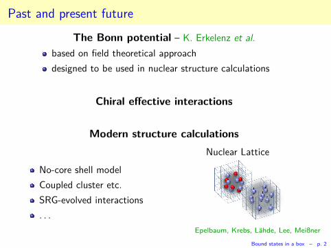
Past and present future
The Bonn potential – K. Erkelenz et al.
based on field theoretical approach
designed to be used in nuclear structure calculations
Chiral effective interactions
Modern structure calculations
No-core shell model
Coupled cluster etc.
SRG-evolved interactions
. . .
Nuclear Lattice
Epelbaum, Krebs, Lahde, Lee, Meißner
Bound states in a box – p. 2
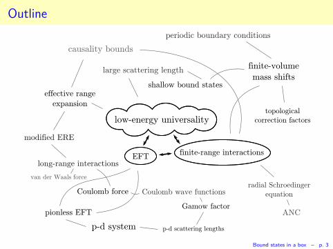
Outline
radial Schroedinger
equation
long-range interactions
Coulomb force
p-d system
ANC
van der Waals force
pionless EFT
effective range
expansion
large scattering length
causality bounds
finite-volume
mass shifts
topological
correction factors
shallow bound states
Coulomb wave functions
Gamow factor
low-energy universality
EFTfinite-range interactions
periodic boundary conditions
modified ERE
p-d scattering lengths
Bound states in a box – p. 3
Prelude
Low-energy universality
and finite-range interactions
Bound states in a box – p. 4
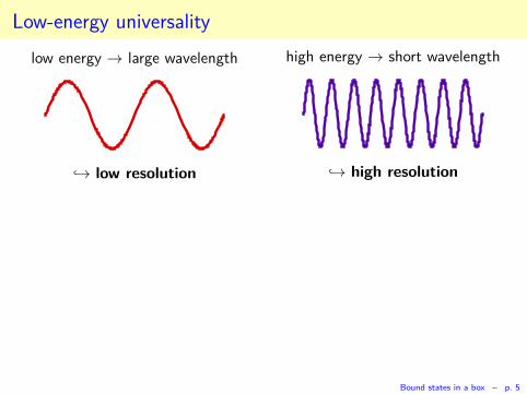
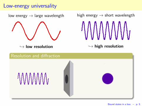
Low-energy universality
low energy → large wavelength
→ low resolution
high energy → short wavelength
→ high resolution
Bound states in a box – p. 5
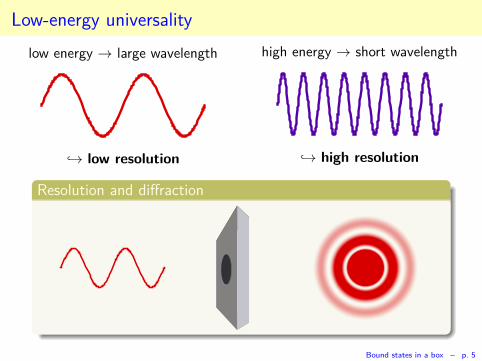
Low-energy universality
low energy → large wavelength
→ low resolution
high energy → short wavelength
→ high resolution
Resolution and diffraction
Bound states in a box – p. 5
Low-energy universality
low energy → large wavelength
→ low resolution
high energy → short wavelength
→ high resolution
Resolution and diffraction
Bound states in a box – p. 5
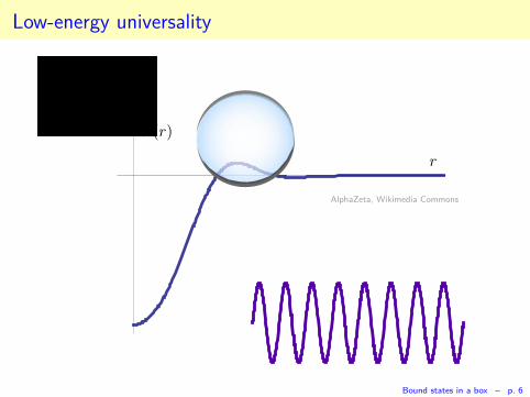
Low-energy universality
r
V (r)
AlphaZeta, Wikimedia Commons
Bound states in a box – p. 6
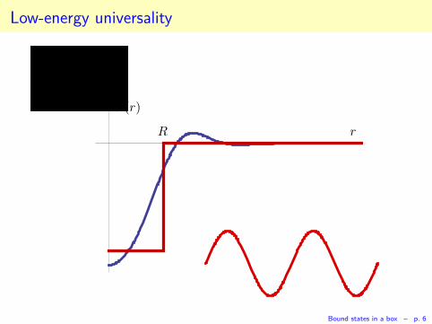
Low-energy universality
R r
V (r)
Bound states in a box – p. 6
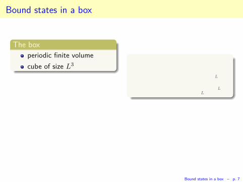
Bound states in a box
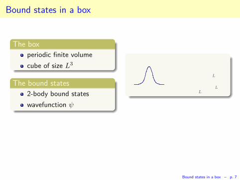
The box
periodic finite volume
cube of size L3
Bound states in a box – p. 7
Bound states in a box
The box
periodic finite volume
cube of size L3
The bound states
2-body bound states
wavefunction ψ
Bound states in a box – p. 7
Bound states in a box
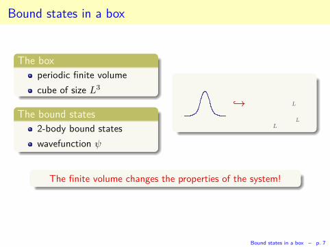
The box
periodic finite volume
cube of size L3
The bound states
2-body bound states
wavefunction ψ
→
The finite volume changes the properties of the system!
Bound states in a box – p. 7
Bound states in a box
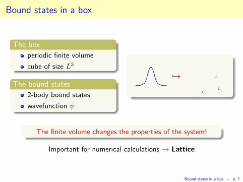
The box
periodic finite volume
cube of size L3
The bound states
2-body bound states
wavefunction ψ
→
The finite volume changes the properties of the system!
Important for numerical calculations → Lattice
Bound states in a box – p. 7
Lattice calculations
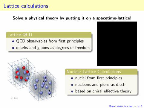
Solve a physical theory by putting it on a spacetime-lattice!
Lattice QCD
QCD observables from first principles
quarks and gluons as degrees of freedom
D. Lee
Nuclear Lattice Calculations
nuclei from first principles
nucleons and pions as d.o.f.
based on chiral effective theory
Bound states in a box – p. 8
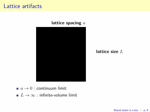
Lattice artifacts
lattice spacing a
lattice size L
a → 0 : continuum limit
L → ∞ : infinite-volume limit
Bound states in a box – p. 9
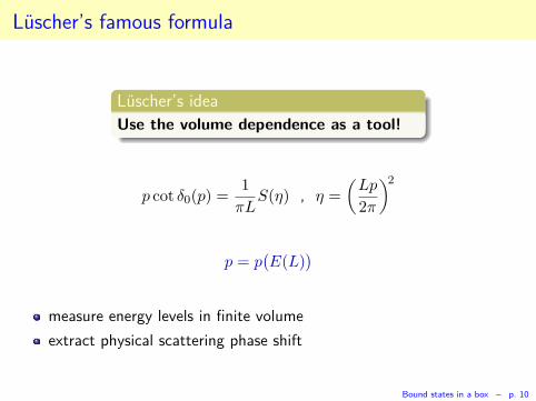
Luscher’s famous formula
Luscher’s idea
Use the volume dependence as a tool!
p cot δ0(p) =1
πLS(η) , η =
(
Lp
2π
)2
p = p(
E(L))
measure energy levels in finite volume
extract physical scattering phase shift
Bound states in a box – p. 10
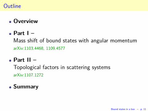
Outline
Overview
Part I –
Mass shift of bound states with angular momentum
arXiv:1103.4468, 1109.4577
Part II –
Topological factors in scattering systems
arXiv:1107.1272
Summary
Bound states in a box – p. 11
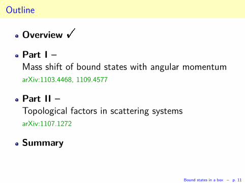
Outline
Overview ✦
Part I –
Mass shift of bound states with angular momentum
arXiv:1103.4468, 1109.4577
Part II –
Topological factors in scattering systems
arXiv:1107.1272
Summary
Bound states in a box – p. 11
Part I
Mass shift of bound states with angular momentum
Luscher’s result for S-waves
Bound states in a finite volume
General result for arbitrary partial waves
Sign of the mass shift
Numerical tests
Bound states in a box – p. 12
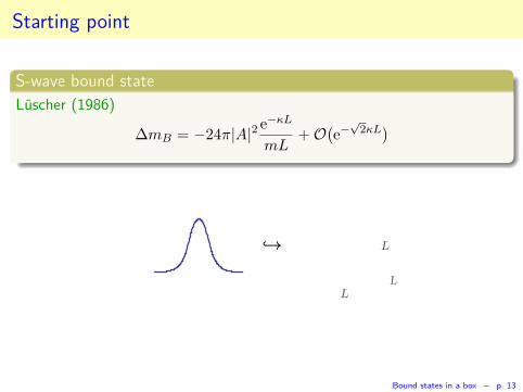
Starting point
S-wave bound state
Luscher (1986)
∆mB = −24π|A|2 e−κL
mL+ O(
e−√
2κL)
→
Bound states in a box – p. 13
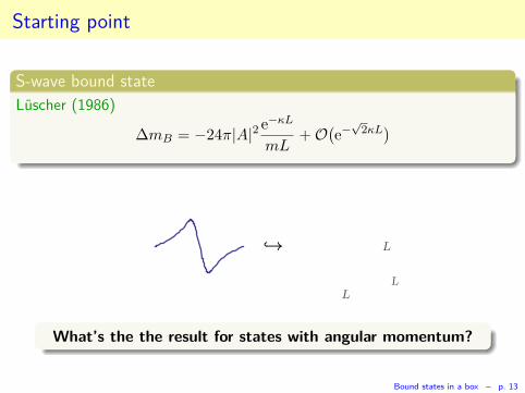
Starting point
S-wave bound state
Luscher (1986)
∆mB = −24π|A|2 e−κL
mL+ O(
e−√
2κL)
→
What’s the the result for states with angular momentum?
Bound states in a box – p. 13
Why care about higher partial waves?
Bound states in a box – p. 14

Halo nuclei
single nucleon weakly bound to atight core
nucleus by Cam-Ann, Wikimedia Commons
Bound states in a box – p. 15

Halo nuclei
single nucleon weakly bound to atight core
can be described as an effective2-body state
nucleus by Cam-Ann, Wikimedia Commons
Bound states in a box – p. 15
Halo nuclei
single nucleon weakly bound to atight core
can be described as an effective2-body state
nucleus by Cam-Ann, Wikimedia Commons
Halo-EFT
expansion in Rcore/Rhalo → effective field theory
Bound states in a box – p. 15
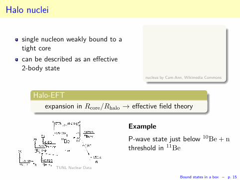
Halo nuclei
single nucleon weakly bound to atight core
can be described as an effective2-body state
nucleus by Cam-Ann, Wikimedia Commons
Halo-EFT
expansion in Rcore/Rhalo → effective field theory
Example
P-wave state just below 10Be + nthreshold in 11Be
TUNL Nuclear Data
Bound states in a box – p. 15
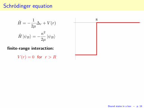
Schrodinger equation
H = − 1
2µ∆r + V (r)
H |ψB〉 = −κ2
2µ|ψB〉
finite-range interaction:
V (r) = 0 for r > R
R
Bound states in a box – p. 16
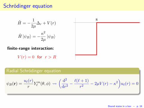
Schrodinger equation
H = − 1
2µ∆r + V (r)
H |ψB〉 = −κ2
2µ|ψB〉
finite-range interaction:
V (r) = 0 for r > R
R
Radial Schrodinger equation
ψB(r) =uℓ(r)
rY m
ℓ (θ, φ)
(
d2
dr2− ℓ(ℓ+ 1)
r2− 2µV (r) − κ2
)
uℓ(r) = 0
Bound states in a box – p. 16
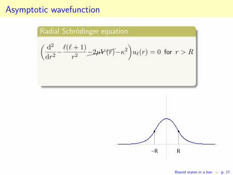
Asymptotic wavefunction
Radial Schrodinger equation
(
d2
dr2− ℓ(ℓ+ 1)
r2 ✘✘✘✘✘−2µV (r)−κ2
)
uℓ(r) = 0 for r > R
æ æ
-R R
Bound states in a box – p. 17
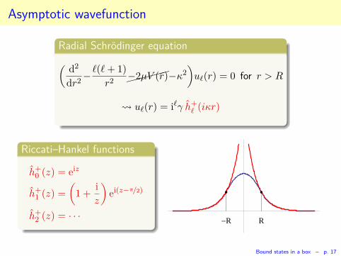
Asymptotic wavefunction
Radial Schrodinger equation
(
d2
dr2− ℓ(ℓ+ 1)
r2 ✘✘✘✘✘−2µV (r)−κ2
)
uℓ(r) = 0 for r > R
uℓ(r) = iℓγ h+ℓ (iκr)
Riccati–Hankel functions
h+0 (z) = eiz
h+1 (z) =
(
1 +i
z
)
ei(z−π/2)
h+2 (z) = · · ·
æ æ
-R R
Bound states in a box – p. 17
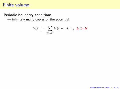
Finite volume
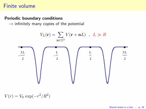
Periodic boundary conditions
→ infinitely many copies of the potential
VL(r) =∑
n∈Z3
V (r + nL) , L ≫ R
Bound states in a box – p. 18
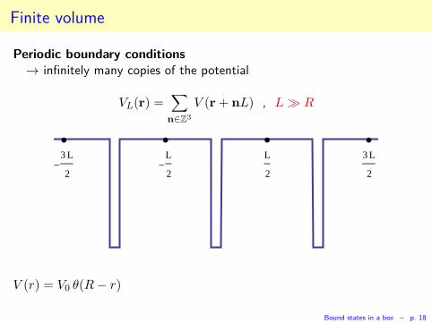
Finite volume
Periodic boundary conditions
→ infinitely many copies of the potential
VL(r) =∑
n∈Z3
V (r + nL) , L ≫ R
æ æ æ æ
-
3 L
2-
L
2
L
2
3 L
2
V (r) = V0 θ(R− r)
Bound states in a box – p. 18
Finite volume
Periodic boundary conditions
→ infinitely many copies of the potential
VL(r) =∑
n∈Z3
V (r + nL) , L ≫ R
æ æ æ æ
-
3 L
2-
L
2
L
2
3 L
2
V (r) = V0 exp(−r2/R2)
Bound states in a box – p. 18

Finite volume
Periodic boundary conditions
→ infinitely many copies of the potential
VL(r) =∑
n∈Z3
V (r + nL) , L ≫ R
æ æ æ æ
-
3 L
2-
L
2
L
2
3 L
2
V (r) = V0exp(−r/R)
r
Bound states in a box – p. 18
Finite volume
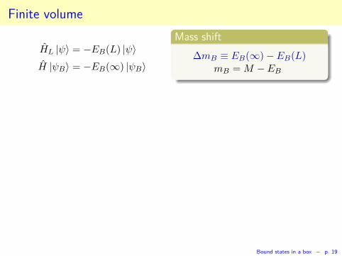
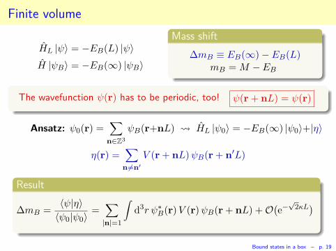
HL |ψ〉 = −EB(L) |ψ〉H |ψB〉 = −EB(∞) |ψB〉
Mass shift
∆mB ≡ EB(∞) − EB(L)mB = M − EB
Bound states in a box – p. 19
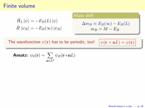
Finite volume
HL |ψ〉 = −EB(L) |ψ〉H |ψB〉 = −EB(∞) |ψB〉
Mass shift
∆mB ≡ EB(∞) − EB(L)mB = M − EB
The wavefunction ψ(r) has to be periodic, too! ψ(r + nL) = ψ(r)
Ansatz: ψ0(r) =∑
n∈Z3
ψB(r+nL)
Bound states in a box – p. 19
Finite volume
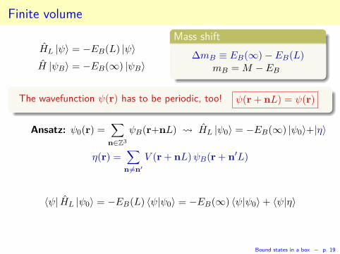
HL |ψ〉 = −EB(L) |ψ〉H |ψB〉 = −EB(∞) |ψB〉
Mass shift
∆mB ≡ EB(∞) − EB(L)mB = M − EB
The wavefunction ψ(r) has to be periodic, too! ψ(r + nL) = ψ(r)
Ansatz: ψ0(r) =∑
n∈Z3
ψB(r+nL) HL |ψ0〉 = −EB(∞) |ψ0〉+|η〉
η(r) =∑
n6=n′
V (r + nL)ψB(r + n′L)
〈ψ| HL |ψ0〉 = −EB(L) 〈ψ|ψ0〉 = −EB(∞) 〈ψ|ψ0〉 + 〈ψ|η〉
Bound states in a box – p. 19
Finite volume
HL |ψ〉 = −EB(L) |ψ〉H |ψB〉 = −EB(∞) |ψB〉
Mass shift
∆mB ≡ EB(∞) − EB(L)mB = M − EB
The wavefunction ψ(r) has to be periodic, too! ψ(r + nL) = ψ(r)
Ansatz: ψ0(r) =∑
n∈Z3
ψB(r+nL) HL |ψ0〉 = −EB(∞) |ψ0〉+|η〉
η(r) =∑
n6=n′
V (r + nL)ψB(r + n′L)
〈ψ| HL |ψ0〉 = −EB(L) 〈ψ|ψ0〉 = −EB(∞) 〈ψ|ψ0〉 + 〈ψ|η〉Result
∆mB =〈ψ|η〉
〈ψ0|ψ0〉 =∑
|n|=1
∫
d3r ψ∗B(r)V (r)ψB(r + nL) + O(
e−√
2κL)
Bound states in a box – p. 19
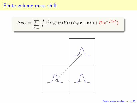
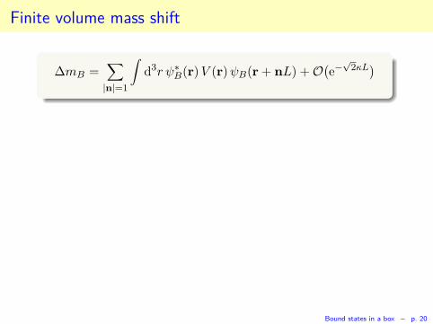
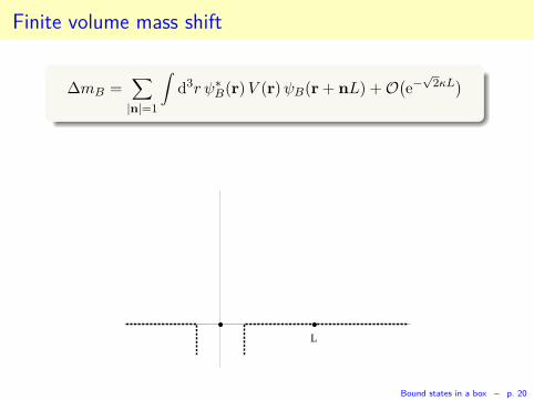
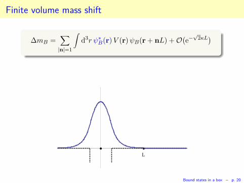
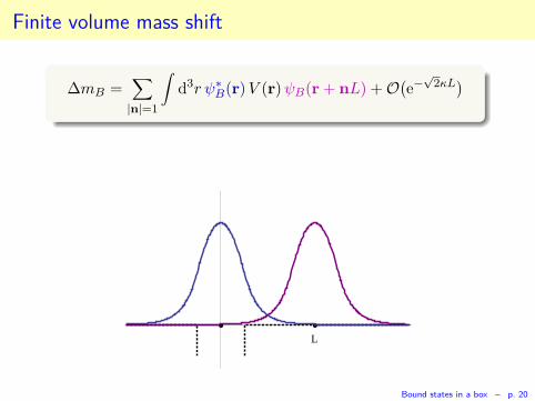
Finite volume mass shift
∆mB =∑
|n|=1
∫
d3r ψ∗B(r)V (r)ψB(r + nL) + O(
e−√
2κL)
Bound states in a box – p. 20
Finite volume mass shift
∆mB =∑
|n|=1
∫
d3r ψ∗B(r)V (r)ψB(r + nL) + O(
e−√
2κL)
Bound states in a box – p. 20
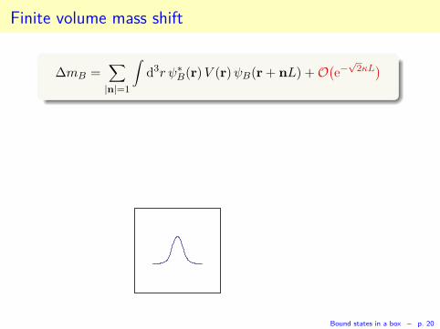
Finite volume mass shift
∆mB =∑
|n|=1
∫
d3r ψ∗B(r)V (r)ψB(r + nL) + O(
e−√
2κL)
Bound states in a box – p. 20
Finite volume mass shift
∆mB =∑
|n|=1
∫
d3r ψ∗B(r)V (r)ψB(r + nL) + O(
e−√
2κL)
Bound states in a box – p. 20
Finite volume mass shift
∆mB =∑
|n|=1
∫
d3r ψ∗B(r)V (r)ψB(r + nL) + O(
e−√
2κL)
Bound states in a box – p. 20

Finite volume mass shift
∆mB =∑
|n|=1
∫
d3r ψ∗B(r)V (r)ψB(r + nL) + O(
e−√
2κL)
Bound states in a box – p. 20
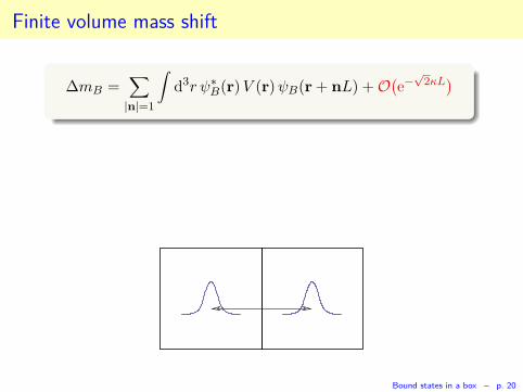
Finite volume mass shift
∆mB =∑
|n|=1
∫
d3r ψ∗B(r)V (r)ψB(r + nL) + O(
e−√
2κL)
æ æ
L
Bound states in a box – p. 20
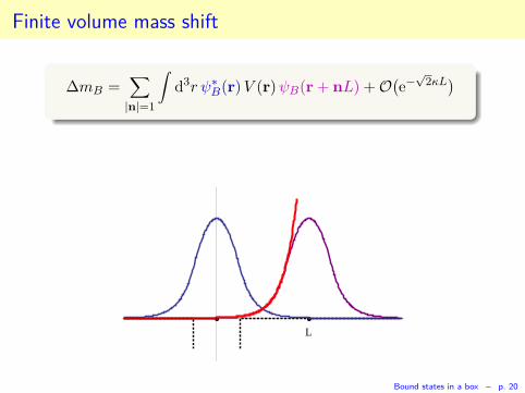
Finite volume mass shift
∆mB =∑
|n|=1
∫
d3r ψ∗B(r)V (r)ψB(r + nL) + O(
e−√
2κL)
æ æ
L
Bound states in a box – p. 20
Finite volume mass shift
∆mB =∑
|n|=1
∫
d3r ψ∗B(r)V (r)ψB(r + nL) + O(
e−√
2κL)
æ æ
L
Bound states in a box – p. 20
Finite volume mass shift
∆mB =∑
|n|=1
∫
d3r ψ∗B(r)V (r)ψB(r + nL) + O(
e−√
2κL)
æ æ
L
Bound states in a box – p. 20
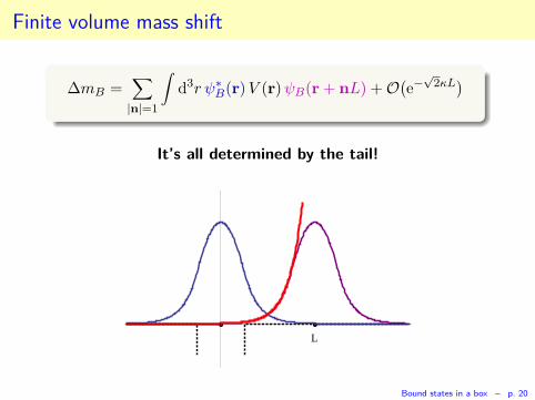
Finite volume mass shift
∆mB =∑
|n|=1
∫
d3r ψ∗B(r)V (r)ψB(r + nL) + O(
e−√
2κL)
It’s all determined by the tail!
æ æ
L
Bound states in a box – p. 20
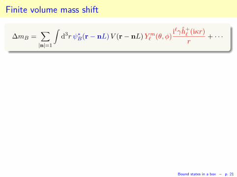
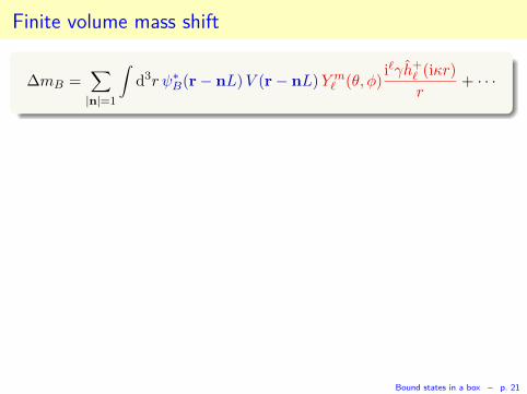
Finite volume mass shift
∆mB =∑
|n|=1
∫
d3r ψ∗B(r − nL)V (r − nL)Y m
ℓ (θ, φ)iℓγh+
ℓ (iκr)
r+ · · ·
Bound states in a box – p. 21
Finite volume mass shift
∆mB =∑
|n|=1
∫
d3r ψ∗B(r − nL)V (r − nL)Y m
ℓ (θ, φ)iℓγh+
ℓ (iκr)
r+ · · ·
Bound states in a box – p. 21
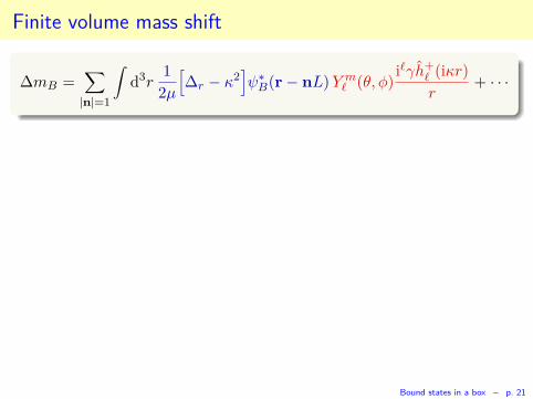
Finite volume mass shift
∆mB =∑
|n|=1
∫
d3r1
2µ
[
∆r − κ2]
ψ∗B(r − nL)Y m
ℓ (θ, φ)iℓγh+
ℓ (iκr)
r+ · · ·
Bound states in a box – p. 21
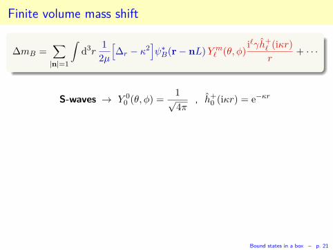
Finite volume mass shift
∆mB =∑
|n|=1
∫
d3r1
2µ
[
∆r − κ2]
ψ∗B(r − nL)Y m
ℓ (θ, φ)iℓγh+
ℓ (iκr)
r+ · · ·
S-waves → Y 00 (θ, φ) =
1√4π
, h+0 (iκr) = e−κr
Bound states in a box – p. 21
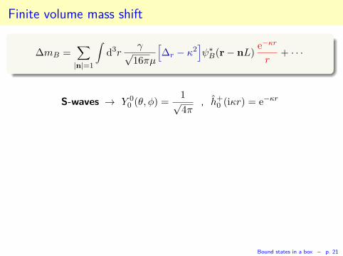
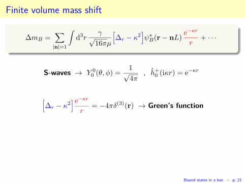
Finite volume mass shift
∆mB =∑
|n|=1
∫
d3rγ√
16πµ
[
∆r − κ2]
ψ∗B(r − nL)
e−κr
r+ · · ·
S-waves → Y 00 (θ, φ) =
1√4π
, h+0 (iκr) = e−κr
Bound states in a box – p. 21
Finite volume mass shift
∆mB =∑
|n|=1
∫
d3rγ√
16πµ
[
∆r − κ2]
ψ∗B(r − nL)
e−κr
r+ · · ·
S-waves → Y 00 (θ, φ) =
1√4π
, h+0 (iκr) = e−κr
[
∆r − κ2]e−κr
r= −4πδ(3)(r) → Green’s function
Bound states in a box – p. 21
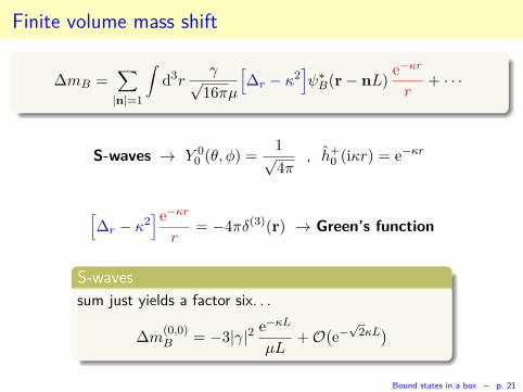
Finite volume mass shift
∆mB =∑
|n|=1
∫
d3rγ√
16πµ
[
∆r − κ2]
ψ∗B(r − nL)
e−κr
r+ · · ·
S-waves → Y 00 (θ, φ) =
1√4π
, h+0 (iκr) = e−κr
[
∆r − κ2]e−κr
r= −4πδ(3)(r) → Green’s function
S-waves
sum just yields a factor six. . .
∆m(0,0)B = −3|γ|2 e−κL
µL+ O(
e−√
2κL)
Bound states in a box – p. 21
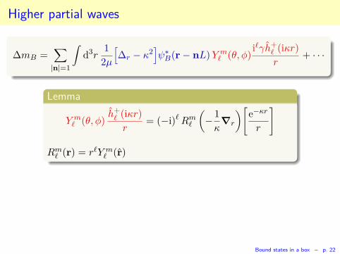
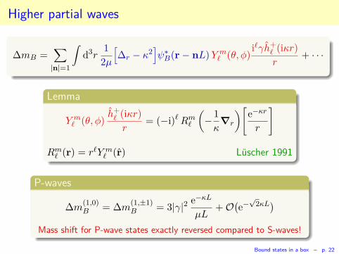
Higher partial waves
∆mB =∑
|n|=1
∫
d3r1
2µ
[
∆r − κ2]
ψ∗B(r − nL)Y m
ℓ (θ, φ)iℓγh+
ℓ (iκr)
r+ · · ·
Lemma
Y mℓ (θ, φ)
h+ℓ (iκr)
r= (−i)ℓRm
ℓ
(
− 1
κ∇r
)
[
e−κr
r
]
Rmℓ (r) = rℓY m
ℓ (r)
Bound states in a box – p. 22
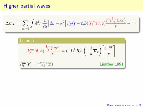
Higher partial waves
∆mB =∑
|n|=1
∫
d3r1
2µ
[
∆r − κ2]
ψ∗B(r − nL)Y m
ℓ (θ, φ)iℓγh+
ℓ (iκr)
r+ · · ·
Lemma
Y mℓ (θ, φ)
h+ℓ (iκr)
r= (−i)ℓRm
ℓ
(
− 1
κ∇r
)
[
e−κr
r
]
Rmℓ (r) = rℓY m
ℓ (r) Luscher 1991
Bound states in a box – p. 22
Higher partial waves
∆mB =∑
|n|=1
∫
d3r1
2µ
[
∆r − κ2]
ψ∗B(r − nL)Y m
ℓ (θ, φ)iℓγh+
ℓ (iκr)
r+ · · ·
Lemma
Y mℓ (θ, φ)
h+ℓ (iκr)
r= (−i)ℓRm
ℓ
(
− 1
κ∇r
)
[
e−κr
r
]
Rmℓ (r) = rℓY m
ℓ (r) Luscher 1991
P-waves
∆m(1,0)B = ∆m
(1,±1)B = 3|γ|2 e−κL
µL+ O(
e−√
2κL)
Mass shift for P-wave states exactly reversed compared to S-waves!
Bound states in a box – p. 22
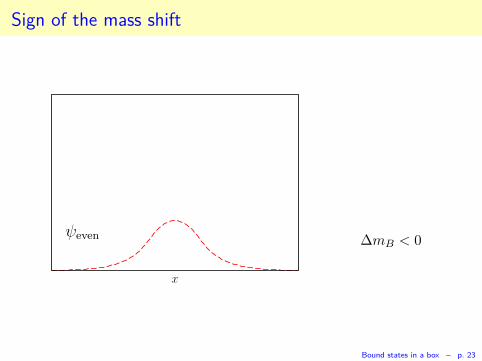
Sign of the mass shift
x
ψeven ∆mB < 0
Bound states in a box – p. 23

Sign of the mass shift
x
ψeven ∆mB < 0
Bound states in a box – p. 23
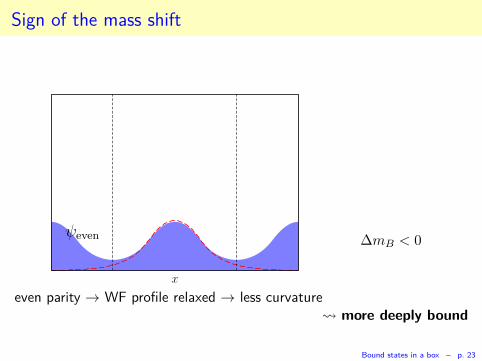
Sign of the mass shift
x
ψeven ∆mB < 0
even parity → WF profile relaxed → less curvature more deeply bound
Bound states in a box – p. 23
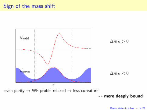
Sign of the mass shift
x
ψeven
ψodd∆mB > 0
∆mB < 0
even parity → WF profile relaxed → less curvature more deeply bound
Bound states in a box – p. 23
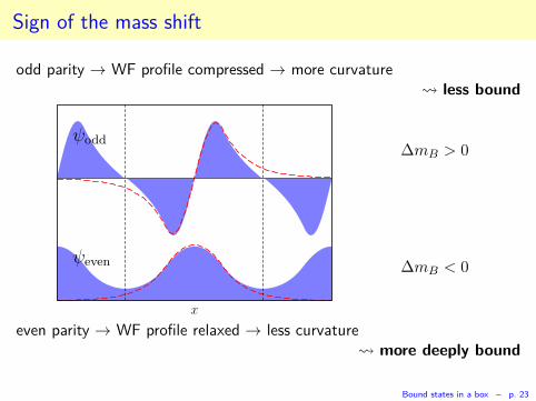
Sign of the mass shift
odd parity → WF profile compressed → more curvature less bound
x
ψeven
ψodd∆mB > 0
∆mB < 0
even parity → WF profile relaxed → less curvature more deeply bound
Bound states in a box – p. 23
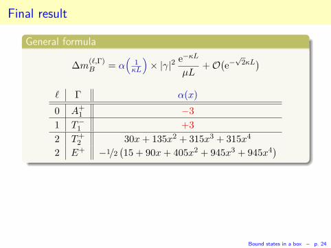
Final result
General formula
∆m(ℓ,Γ)B = α
(
1κL
)
× |γ|2 e−κL
µL+ O(
e−√
2κL)
ℓ Γ α(x)
0 A+1 −3
1 T−1 +3
2 T+2 30x+ 135x2 + 315x3 + 315x4
2 E+ −1/2(
15 + 90x+ 405x2 + 945x3 + 945x4)
Bound states in a box – p. 24
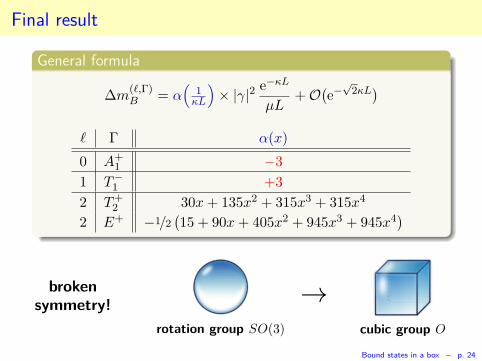
Final result
General formula
∆m(ℓ,Γ)B = α
(
1κL
)
× |γ|2 e−κL
µL+ O(
e−√
2κL)
ℓ Γ α(x)
0 A+1 −3
1 T−1 +3
2 T+2 30x+ 135x2 + 315x3 + 315x4
2 E+ −1/2(
15 + 90x+ 405x2 + 945x3 + 945x4)
broken
symmetry!
rotation group SO(3)
→cubic group O
Bound states in a box – p. 24
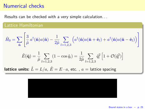
Numerical checks
Results can be checked with a very simple calculation. . .
Lattice Hamiltonian
H0 =∑
n
3
µa†(n)a(n) − 1
2µ
∑
l=1,2,3
(
a†(n)a(n + el) + a†(n)a(n − el))
E(q) =1
µ
∑
l=1,2,3
(1 − cos qi) =1
2µ
∑
l=1,2,3
q2l
[
1 + O(q2l )
]
lattice units: L = L/a, E = E · a, etc. , a = lattice spacing
Bound states in a box – p. 25
Numerical checks
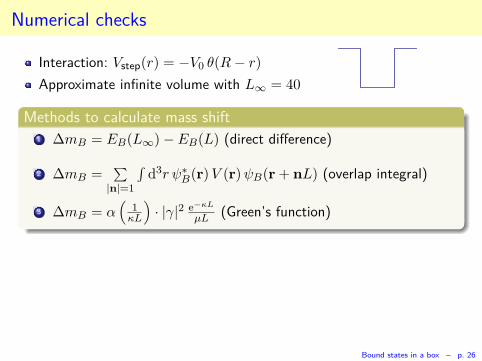
Interaction: Vstep(r) = −V0 θ(R− r)
Approximate infinite volume with L∞ = 40
Methods to calculate mass shift
1 ∆mB = EB(L∞) − EB(L) (direct difference)
2 ∆mB =∑
|n|=1
∫
d3r ψ∗B(r)V (r)ψB(r + nL) (overlap integral)
3 ∆mB = α(
1κL
)
· |γ|2 e−κL
µL (Green’s function)
Bound states in a box – p. 26
Numerical checks
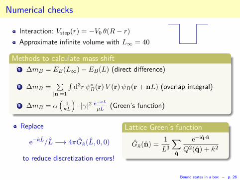
Interaction: Vstep(r) = −V0 θ(R− r)
Approximate infinite volume with L∞ = 40
Methods to calculate mass shift
1 ∆mB = EB(L∞) − EB(L) (direct difference)
2 ∆mB =∑
|n|=1
∫
d3r ψ∗B(r)V (r)ψB(r + nL) (overlap integral)
3 ∆mB = α(
1κL
)
· |γ|2 e−κL
µL (Green’s function)
Replace
e−κL/L −→ 4πGκ(L, 0, 0)
to reduce discretization errors!
Lattice Green’s function
Gκ(n) =1
L3
∑
q
e−iq·n
Q2(q) + κ2
Bound states in a box – p. 26
Numerical checks
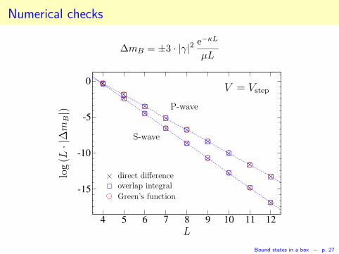
∆mB = ±3 · |γ|2 e−κL
µL
4 5 6 7 8 9 10 11 12
-15
-10
-5
0V = Vstep
S-wave
P-wave
L
log(L
·|∆m
B|)
direct differenceoverlap integral
Green’s function
Bound states in a box – p. 27
Numerical checks
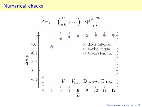
∆mB =
(
30
κL+ · · ·
)
· |γ|2 e−κL
µL
4 5 6 7 8 9 10 11 12
-0.5
-0.4
-0.3
-0.2
-0.1
0
V = Vstep, D-wave, E rep.
L
∆m
B
direct differenceoverlap integral
Green’s function
Bound states in a box – p. 28
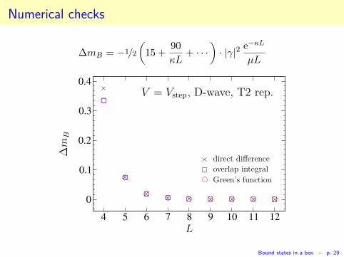
Numerical checks
∆mB = −1/2
(
15 +90
κL+ · · ·
)
· |γ|2 e−κL
µL
4 5 6 7 8 9 10 11 12
0
0.1
0.2
0.3
0.4
V = Vstep, D-wave, T2 rep.
L
∆m
B
direct differenceoverlap integral
Green’s function
Bound states in a box – p. 29
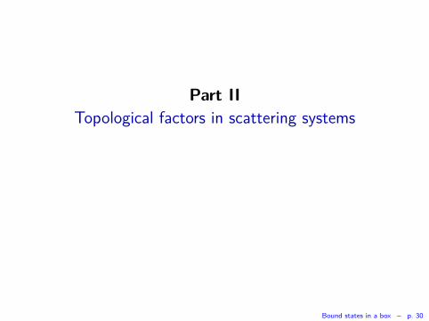
Part II
Topological factors in scattering systems
Bound states in a box – p. 30
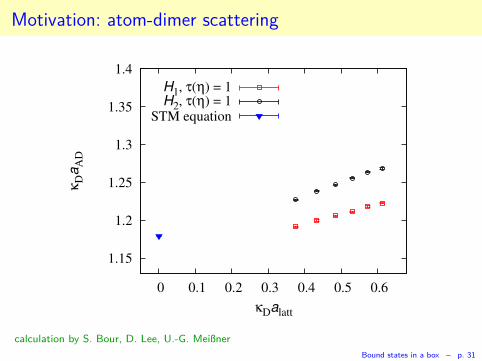
Motivation: atom-dimer scattering
1.15
1.2
1.25
1.3
1.35
1.4
0 0.1 0.2 0.3 0.4 0.5 0.6
κDa
AD
κDalatt
H1, τ(η) = 1H2, τ(η) = 1
STM equation
calculation by S. Bour, D. Lee, U.-G. Meißner
Bound states in a box – p. 31
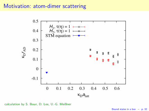
Motivation: atom-dimer scattering
-0.1
0
0.1
0.2
0.3
0.4
0.5
0 0.1 0.2 0.3 0.4 0.5 0.6
κDr A
D
κDalatt
H1, τ(η) = 1H2, τ(η) = 1
STM equation
calculation by S. Bour, D. Lee, U.-G. Meißner
Bound states in a box – p. 32
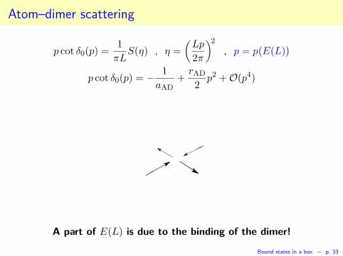
Atom–dimer scattering
p cot δ0(p) =1
πLS(η) , η =
(
Lp
2π
)2
, p = p(
E(L))
p cot δ0(p) = − 1
aAD+rAD
2p2 + O(p4)
A part of E(L) is due to the binding of the dimer!
Bound states in a box – p. 33
Part II
Topological factors in scattering systems
Motivation ✦
Moving bound states in a finite volume
Mass shift for twisted boundary conditions
Corrections for scattering states
Conclusion: corrected atom-dimer results
Bound states in a box – p. 34
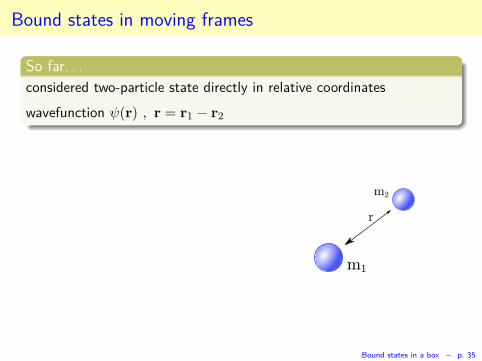
Bound states in moving frames
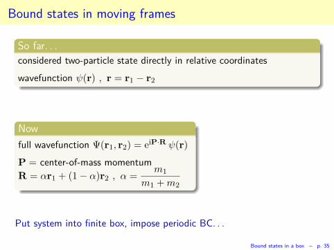
So far. . .
considered two-particle state directly in relative coordinates
wavefunction ψ(r) , r = r1 − r2
m1
m2
r
Bound states in a box – p. 35
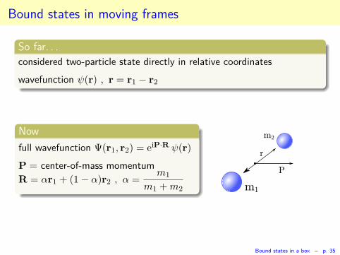
Bound states in moving frames
So far. . .
considered two-particle state directly in relative coordinates
wavefunction ψ(r) , r = r1 − r2
Now
full wavefunction Ψ(r1, r2) = eiP·R ψ(r)
P = center-of-mass momentum
R = αr1 + (1 − α)r2 , α =m1
m1 +m2 m1
m2
r
P
Bound states in a box – p. 35
Bound states in moving frames
So far. . .
considered two-particle state directly in relative coordinates
wavefunction ψ(r) , r = r1 − r2
Now
full wavefunction Ψ(r1, r2) = eiP·R ψ(r)
P = center-of-mass momentum
R = αr1 + (1 − α)r2 , α =m1
m1 +m2 m1
m2
r
P
L
L
Put system into finite box, impose periodic BC. . .
Bound states in a box – p. 35
Twisted boundary conditions
m1
m2
r
P
L
L
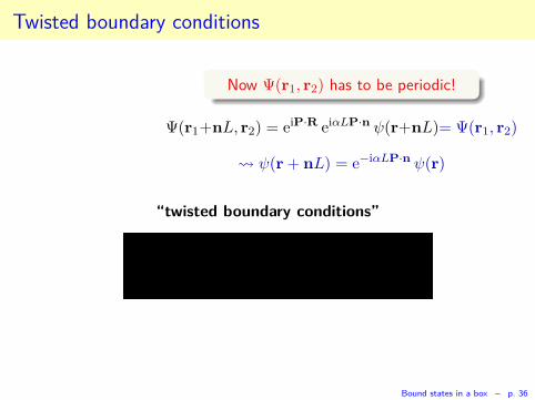
Now Ψ(r1, r2) has to be periodic!
Ψ(r1+nL, r2) = eiP·R eiαLP·n ψ(r+nL)= Ψ(r1, r2)
ψ(r + nL) = e−iαLP·n ψ(r)
“twisted boundary conditions”
Bound states in a box – p. 36
Twisted boundary conditions
m1
m2
r
P
L
L
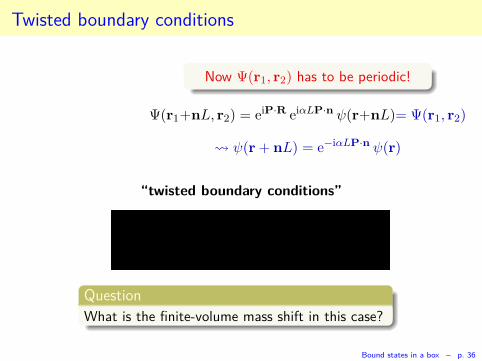
Now Ψ(r1, r2) has to be periodic!
Ψ(r1+nL, r2) = eiP·R eiαLP·n ψ(r+nL)= Ψ(r1, r2)
ψ(r + nL) = e−iαLP·n ψ(r)
“twisted boundary conditions”
Question
What is the finite-volume mass shift in this case?
Bound states in a box – p. 36
Mass shift for twisted boundary conditions
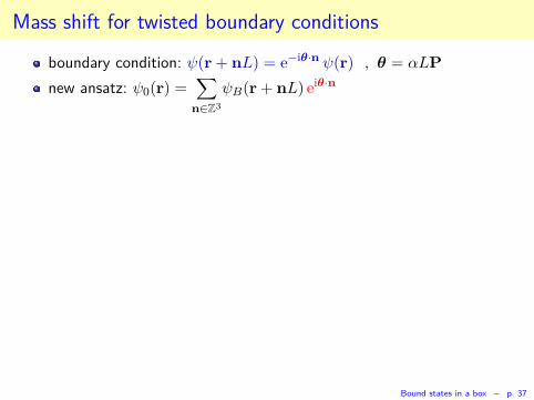
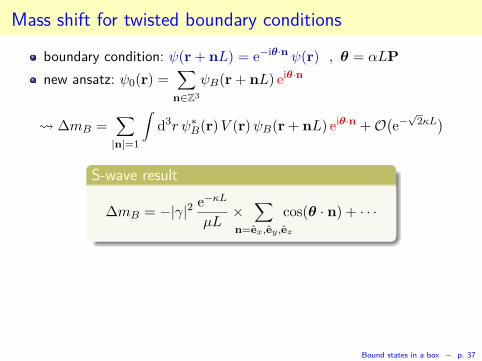
boundary condition: ψ(r + nL) = e−iθ·n ψ(r) , θ = αLP
new ansatz: ψ0(r) =∑
n∈Z3
ψB(r + nL) eiθ·n
✦
Bound states in a box – p. 37
Mass shift for twisted boundary conditions
boundary condition: ψ(r + nL) = e−iθ·n ψ(r) , θ = αLP
new ansatz: ψ0(r) =∑
n∈Z3
ψB(r + nL) eiθ·n
∆mB =∑
|n|=1
∫
d3r ψ∗B(r)V (r)ψB(r + nL) eiθ·n + O(
e−√
2κL)
S-wave result
∆mB = −|γ|2 e−κL
µL×
∑
n=ex,ey ,ez
cos(θ · n) + · · ·
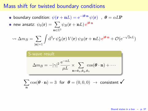
∑
n
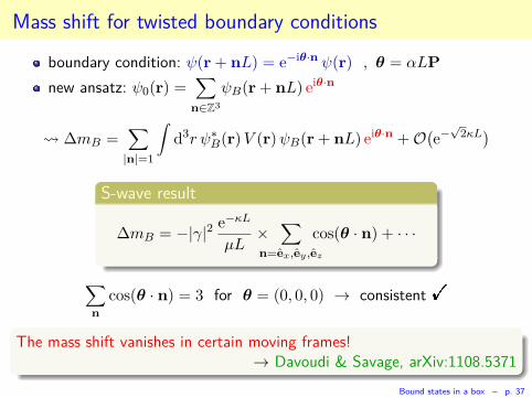
cos(θ · n) = 3 for θ = (0, 0, 0) → consistent ✦
Bound states in a box – p. 37
Mass shift for twisted boundary conditions
boundary condition: ψ(r + nL) = e−iθ·n ψ(r) , θ = αLP
new ansatz: ψ0(r) =∑
n∈Z3
ψB(r + nL) eiθ·n
∆mB =∑
|n|=1
∫
d3r ψ∗B(r)V (r)ψB(r + nL) eiθ·n + O(
e−√
2κL)
S-wave result
∆mB = −|γ|2 e−κL
µL×
∑
n=ex,ey ,ez
cos(θ · n) + · · ·
∑
n
cos(θ · n) = 3 for θ = (0, 0, 0) → consistent ✦
The mass shift vanishes in certain moving frames!→ Davoudi & Savage, arXiv:1108.5371
Bound states in a box – p. 37
Scattering states
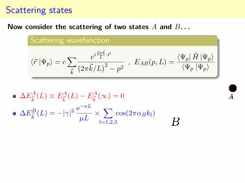
Now consider the scattering of two states A and B. . .
Scattering wavefunction
〈~r |Ψp〉 = c∑
~k
ei 2π~kL
·~r(
2π~k/L)2 − p2
, EAB(p, L) =〈Ψp| H |Ψp〉
〈Ψp |Ψp〉
∆EA~k
(L) ≡ EA~k
(L) − EA~k
(∞) = 0
∆EB~k
(L) = −|γ|2 e−κL
µL×
∑
l=1,2,3
cos(2παBkl)

Scattering states
Now consider the scattering of two states A and B. . .
Scattering wavefunction
〈~r |Ψp〉 = c∑
~k
ei 2π~kL
·~r(
2π~k/L)2 − p2
, EAB(p, L) =〈Ψp| H |Ψp〉
〈Ψp |Ψp〉
∆EA~k
(L) ≡ EA~k
(L) − EA~k
(∞) = 0
∆EB~k
(L) = −|γ|2 e−κL
µL×
∑
l=1,2,3
cos(2παBkl)
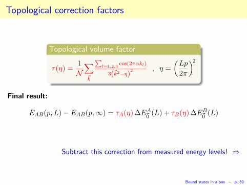
Topological correction factors
Topological volume factor
τ(η) =1
N∑
~k
∑
l=1,2,3cos(2παkl)
3(~k2−η)2 , η =
(
Lp
2π
)2
Final result:
EAB(p, L) − EAB(p,∞) = τA(η) ∆EA~0
(L) + τB(η) ∆EB~0
(L)
Subtract this correction from measured energy levels! ⇒
Bound states in a box – p. 39
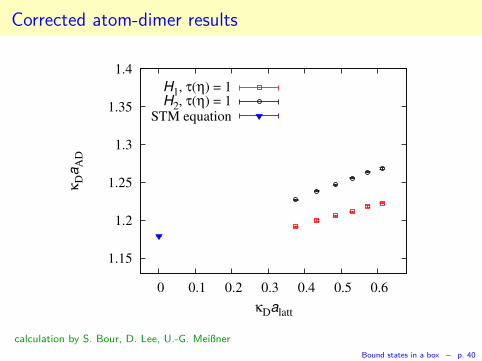
Corrected atom-dimer results
1.15
1.2
1.25
1.3
1.35
1.4
0 0.1 0.2 0.3 0.4 0.5 0.6
κDa
AD
κDalatt
H1, τ(η) = 1H2, τ(η) = 1
STM equation
calculation by S. Bour, D. Lee, U.-G. Meißner
Bound states in a box – p. 40
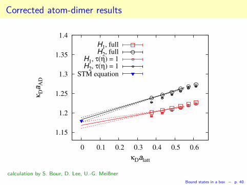
Corrected atom-dimer results
1.15
1.2
1.25
1.3
1.35
1.4
0 0.1 0.2 0.3 0.4 0.5 0.6
κDa
AD
κDalatt
H1, fullH2, full
H1, τ(η) = 1H2, τ(η) = 1
STM equation
calculation by S. Bour, D. Lee, U.-G. Meißner
Bound states in a box – p. 40
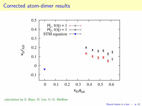
Corrected atom-dimer results
-0.1
0
0.1
0.2
0.3
0.4
0.5
0 0.1 0.2 0.3 0.4 0.5 0.6
κDr A
D
κDalatt
H1, τ(η) = 1H2, τ(η) = 1
STM equation
calculation by S. Bour, D. Lee, U.-G. Meißner
Bound states in a box – p. 41
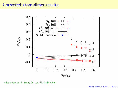
Corrected atom-dimer results
-0.1
0
0.1
0.2
0.3
0.4
0.5
0 0.1 0.2 0.3 0.4 0.5 0.6
κDr A
D
κDalatt
H1, fullH2, full
H1, τ(η) = 1H2, τ(η) = 1
STM equation
calculation by S. Bour, D. Lee, U.-G. Meißner
Bound states in a box – p. 41
The End
Summary
Mass shift can be calculated for bound states with arbitrary ℓ.
Sign of the shift can be related to parity of the states.
Predictions can be tested by numerical calculations.
Mass shift of composite particles has to be corrected for inscattering calculations.
Bound states in a box – p. 42
The End
Summary
Mass shift can be calculated for bound states with arbitrary ℓ.
Sign of the shift can be related to parity of the states.
Predictions can be tested by numerical calculations.
Mass shift of composite particles has to be corrected for inscattering calculations.
***
Thanks for your attention!
Bound states in a box – p. 42