Embed Size (px)
Citation preview
DEVELOPMENT OF WINDBREAKS AS A DUST CONTROL STRATEGY FOR COMMUNITIES IN ARID CLIMATES SUCH AS THE US-MEXICO BORDER REGION
SCERP PROJECT NUMBER: A-04-06 ERIC R. PARDYJAK, UNIVERSITY OF UTAH
PRATHAP RAMAMURTHY, UNIVERSITY OF UTAH
SCOTT SPECKART, UNIVERSITY OF UTAH
INTRODUCTION
Reduction of fugitive dust emissions in arid regions such as those in the US-Mexico border region is of utmost concern to border air quality. Known as fugitive dust, particulate matter generated from the mechanical disturbance of granular crustal material has many sources and is a serious health concern. Sources include but are not limited to: Unpaved roads, construction operations, grazing land, agriculture and mine tailings. PM10 is the criteria pollutant commonly associated with fugitive dust and has been linked with numerous health problems. Illnesses can include lung and heart disease to asthma. Severity can vary from chronic health nuisances to death (Samet et al. 1998). Because it is not emitted as part of a regulated airstream, reductions in fugitive dust emissions have proven difficult. Air quality officials in the southwest are dissatisfied with the available options for controlling vehicle generated fugitive dust since water-based treatments are often impractical in arid climates. Previous SCERP-funded studies in Doña Ana County, New Mexico have examined the hypothesis that dust traveling near the ground is redeposited when it encounters brush, fences, and small terrain irregularities. A conclusion from this work is that depending upon atmospheric stability (i.e. time of day), vegetative canopies may affect the amount of vehicle-suspended dust that is actually transported sufficient distance to affect local and regional air quality. Other field studies have supported this conclusion. This study seeks to observe if similar results are obtained with an artificial windbreak. The first portion of this report describes windbreak results from a field experiment in Nogales, Sonora, while Appendices 1 and 2 describes the details of a numerical model designed to predict deposition for a wide range of rough surfaces.
RESEARCH OBJECTIVES
The research documented in this report covers a field experiment performed in Nogales, Sonora during the month of May 2006. This experiment uses automotive traffic on an unpaved road as a source of fugitive dust. A computer simulation code that models dust traveling downwind of a dirt road is used as well to describe the characteristics of dust transport in an artificial windbreak. This model is described thoroughly by Pardyjak et al. (submitted October 2007), and, Veranth et al. (submitted Oct. 2007) and are included at the end of this document. Other methods of describing dust transport, such as Gaussian Plume models, and mass fraction advected down wind are utilized. The latter method has been used by Veranth et al. (2003) and Etyemezian et al. (2004).
An objective is to obtain a greater understanding of the principles that one may use to implement an artificial windbreak dust control strategy. Issues such as height and number of rows of windbreaks will be explored. An evaluation of effectiveness of specific dust control strategies is the final objective of this work.
RESEARCH METHODOLOGY/ APPROACHES
Background
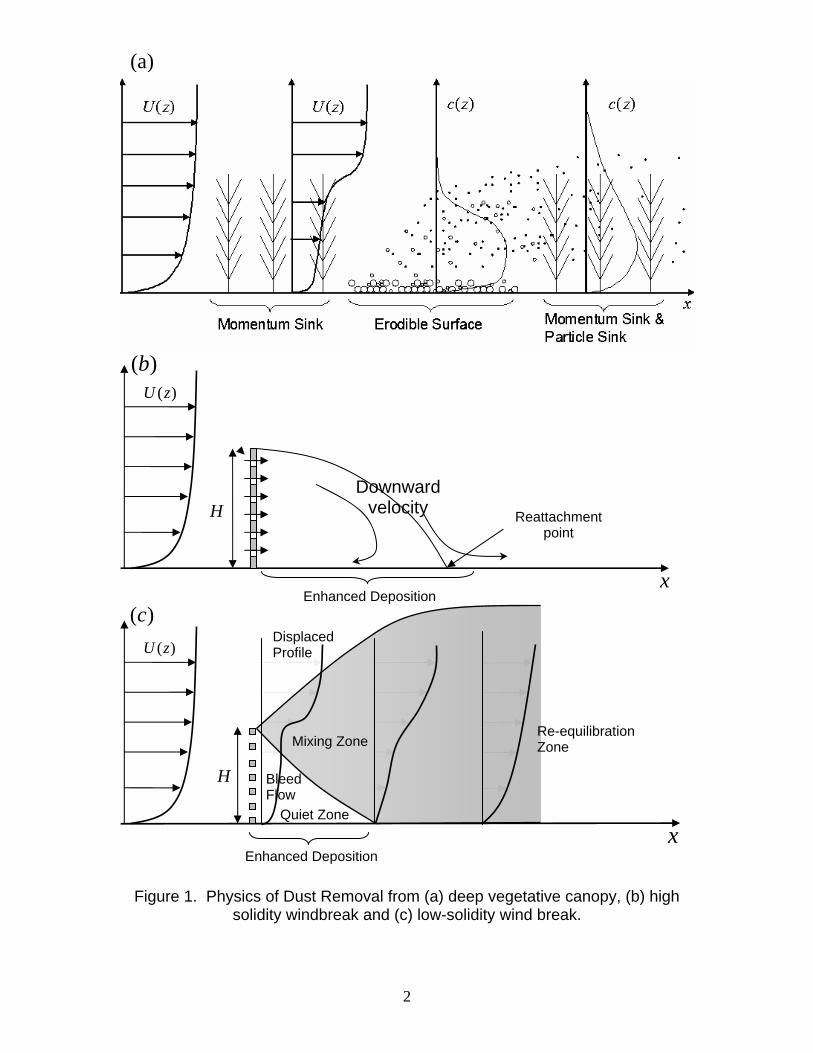
The motivation for the use of vegetative canopies or artificial windbreaks is shown in figure 1. On the left of the figure there is an undisturbed mean velocity profile with wind speeds that typically vary vertically in a logarithmic manner. As the wind encounters vegetation, buildings or an artificial wind break the air near these obstructions slows down and depending on the type of flow the velocity profile takes on a drastically different character. In figure 1a the velocity profile below the vegetative canopy top takes on an exponential profile as noted in Cionco (1965). The new modified exponential profile is deficit in momentum near these obstacles. Similar profiles are observed downwind of windbreaks with low porosity, φ < 0.2, (Fig 1c), while windbreaks with high solidity, (Fig 1b), have recirculating flow with associated strong down ward velocities and reattachment point (McNaughton, 1988).
As wind or vehicles disturb granular material, fugitive dust is emitted into the air stream. If the fugitive dust is emitted into an undisturbed, high momentum logarithmic profile, its residence time near the ground or small obstacles, such as vines or sparse grass will be small (i.e. the PM is quickly advected away and diluted). As a consequence the probability of an appreciable quantity of fugitive dust being redeposited to the ground or small obstacles is small compared to a vegetated case.
2
If the dust is emitted into a slower, highly turbulent, modified exponential profile, the residence time of the dust spent near the ground and other obstacles is much greater thus increasing the probability that a significant amount of dust is redeposited. It is also probable that the concentration of dust in a vegetative canopy or an artificial windbreak would be higher than the air directly above due to this increased residence time characteristic of canopies and wind breaks.
Additional factors also modify fugitive dust transport. For example, dust needs a physical surface for redeposition. Vegetative canopies and artificial wind breaks provide additional surface area for redeposition. Another important factor is atmospheric stability. If the atmosphere is unstable vertical mixing will be promoted. The distribution of the cloud will reach higher elevations far above obstructions and ground. Under these circumstances a lower fraction of fugitive dust would be expected to be redeposited. The converse would be true for stable conditions. Experimentally, this has been observed by three separate experiments. One of these experiments is documented in Veranth et al. (2003) another in Etyemezian et al. (2004) and the final in Veranth et al. (2007).
Experiment Description
The May 2006 Nogales Sonora experiment was performed on the dates of May 25, 28, and 29. These dates corresponded with experiments that contained no fence, a 1 m high fence, and a two meter high fence. This is summarized with times and rate of vehicle traffic in Table 1.Theses dates were determined primarily by meteorological conditions and secondarily by equipment status. The location of the experiment was the Nogales Campus of El Colegio Nacional de Educación Professional Técnica (CONALEP) secondary technical school system. (N 31° 16.644’ W 110° 56.694’). It is located in the southern third of the metropolitan area of Nogales, about 200 or 300 m to the west of the principle street that bisects Nogales. Located to the west and up hill of CONALEP is an unpaved road that is the only access to a large and growing colonia (neighborhood). During the morning and evening rush hours, especially the evening, the CONALEP campus is subject to high levels of fugitive dust from the road. For these reasons, as well as establishing Mexican Collaboration, this site was chosen. The site was characterized as arid with short grasses, about 20-60 cm, for about 10 m downwind of the road.
The experimental set up is shown in figure 2. During the experiment runs the site had winds predominantly from west, south west. After traveling over the unpaved road the dust rich air was intercepted by an array of TSI inc. Dustraks and Campbell Scientific CSAT3 sonic anemometers. The artificial windbreak was an event ski fence from REILIBLE RACING INC, that had an optical porosity = 0.53. It was built using bamboo sticks from
3
the same company. The bamboo sticks were driven into the ground with metal posts. The fence extended 92.2 m to the south and 91.4 m to the north of the half plane containing the ultrasonic anemometers and Dustraks. The physical location of the Dustraks and sonic anemometers is located in Table 2. The Dustraks were equipped with PM10 inlets and sampled at a rate of 1Hz. The Sonic anemometers sampled at a rate of 10 Hz. The artificial wind break was located between the first two Dustrak towers. The first Dustrak tower provided data that indicated the magnitude of dust initial suspended. Location was as close to the road as possible without imposing a safety hazard.
The second tower of Dustraks was less than half a meter from the back (downwind face) of the artificial windbreak. This close location was chosen to provide an accurate concentration data directly behind the windbreak. A 5 m Aluminum tower housed the three ultrasonic anemometers along with two other Dustraks. A final Dustrak tower was located at the downwind side of the test site. Similar configurations were used in the in Veranth et al. (2003) the Etyemezian et al. (2004) and Pardyjak et al. (2006) experiments.
There are many meteorological conditions that must be satisfied to have a successful experiment. One the principle wind direction must be within 60° of flowing perpendicular to the road. The 2 m fence experiment was 20 minutes shorter than the other two experiments because this 60° rule was violated during the final 20 minutes. Another involves the magnitude of wind. A high wind, about 15-20 m/s will suspend dust from sources other than the road. Under these conditions quantifying the effectiveness a windbreak or vegetative canopy would be extremely difficult if not impossible. High winds may also generate erroneous sonic anemometer measurements. Lastly precipitation may greatly reduces the amount of dust suspended by cars, or eliminate it completely.
Owing to the high amount of motor traffic, a continuous line source was assumed in the analysis. The topographical changes in the direction along the road were negligible. The test section of the road used was relatively straight. Because of these conditions, it is possible to also assume the dust transport was relatively two-dimensional. From the array of equipment data were acquired for five different primary variables, namely concentration, wind speed, wind direction, and temperature. 10 minute averages for all of these variables were calculated as an initial step in analysis.
Description of Analysis
Means of the primary variables were calculated using Eq. 1,
4
∫−=
ft
tiifa dttc
ttc )(1 (1)
Where ca Time average of the variable c(t) Instantaneous value of the variable tf Final time of averaging period ti Initial time of averaging period In the case of this experiment, tf – ti = 10 min. A discrete version of this integral is used as described in Chapra and Canale (2002). Averages and standard deviations for each of the three experiments were derived from these 10-minute averages. Many steps of the analysis to follow require continuous profiles. Due to the discrete nature of the equipment array, assumptions and least square regressions are needed to complete the analysis. Due to the hillside nature of the site a planar rotation was needed to adequately analyze the wind data. A thorough treatment is given in Wilczak et al. (2001). In addition a number of meteorological quantities of interest were calculated following Stull (1988). First, the interpolation of vertical wind speed was accomplished by using a logarithmic curve of the form below.
( )⎥⎦
⎤⎢⎣
⎡−⎟⎟
⎠
⎞⎜⎜⎝
⎛= Lz
zzu
zuo
/ln)( * ψκ
(2)
Where Κ Von Karman constant
*u Friction velocity (m/s) zo Aerodynamic roughness length (m) Ψ Stability function Ψ = - 4.7(z/L) (stable conditions)
L Monin-Obukhov length scale (m); ''
3*
TwTg
uL⎟⎠⎞
⎜⎝⎛−
=κ
T mean temperature measure with sonic the anemometer (K)
5
''Tw Kinematic heat flux (m-K/s) Additional information on this profile is included in (Arya 2001). To approximate the vertical concentration profiles, an exponential fit was used as in Veranth et al. (2003). The physical basis and success of Veranth et al. (2003) was the reason this interpolation was used. This profile is defined by the equation below:
)*exp(*)( zBAzc −= Where c(z) The concentration at a given height z The height above the ground A Fitting Parameter B Fitting Parameter A least squares reduction may be used to obtain values for the fitting parameters. These reductions are based upon the 10 minute averaged data. During the majority of the experiment the height of the cloud was consistently located above the highest Dustrak which was located at 5 m. To estimate the top of the cloud a Gaussian Plume model was used. Gaussian Plume Modeling Gaussian Plume Models are used to model pollution dispersion. A thorough treatment and derivation is found in Seinfeld and Pandis (1998). Two forms or the equation exist for near ground transport. One assumes the ground is a perfect absorber and the other assumes it is a perfect reflector. For the purposes of the experiment both models give results that differ less than the experimental variability by more than order of magnitude. The model for a continuous plume is given by Eq. 3 below
⎟⎟⎠
⎞⎜⎜⎝
⎛⎟⎟⎠
⎞⎜⎜⎝
⎛ +−±⎟⎟
⎠
⎞⎜⎜⎝
⎛ −−⎟
⎟⎠
⎞⎜⎜⎝
⎛−= 2
2
2
2
2
2
2)(exp
2)(exp*
2exp
2),,(
zzyzy
hzhzyU
qzyxcσσσσσπ
(3)
Where q Source strength g/s σy Standard deviation relating concentration and position in span wise
direction
6
σz Standard deviation relating concentration and position in vertical direction
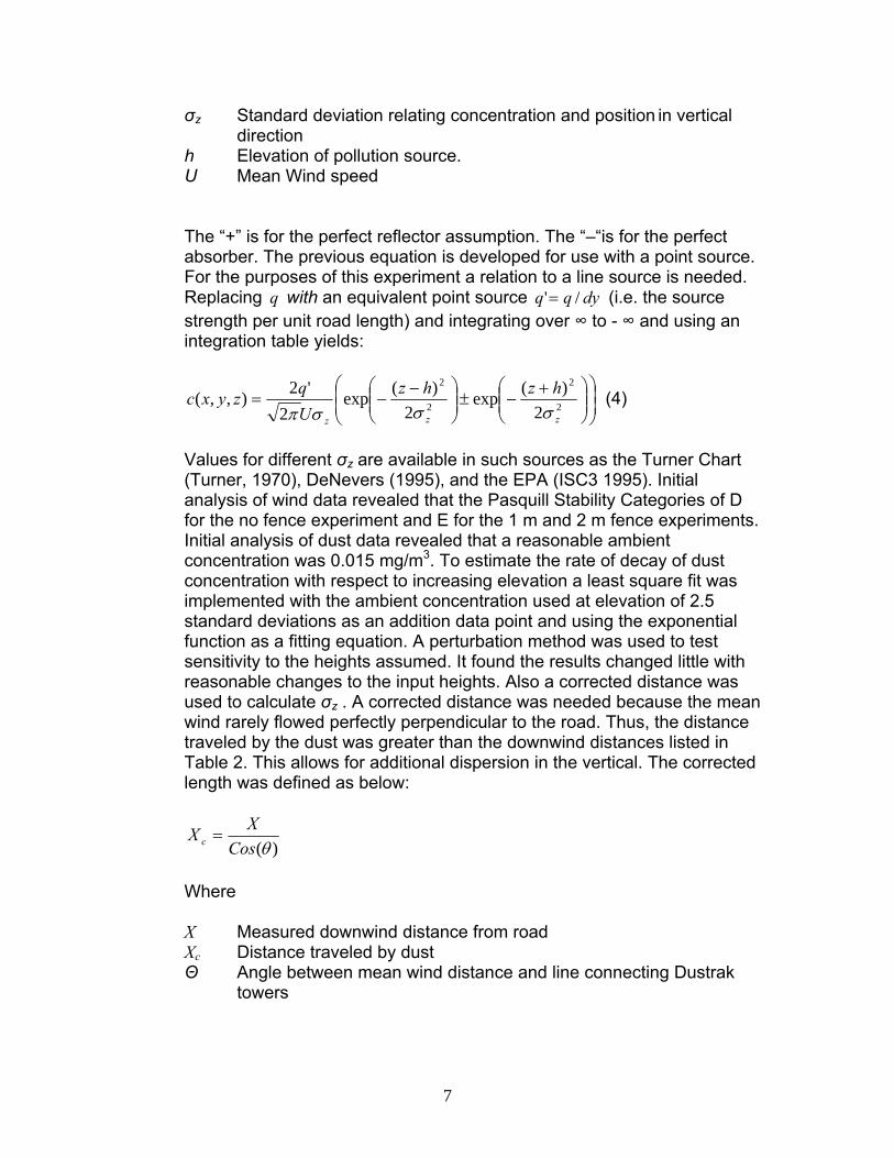
h Elevation of pollution source. U Mean Wind speed The “+” is for the perfect reflector assumption. The “–“is for the perfect absorber. The previous equation is developed for use with a point source. For the purposes of this experiment a relation to a line source is needed. Replacing with an equivalent point source q dyqq /'= (i.e. the source strength per unit road length) and integrating over ∞ to - ∞ and using an integration table yields:
⎟⎟⎠
⎞⎜⎜⎝
⎛⎟⎟⎠
⎞⎜⎜⎝
⎛ +−±⎟⎟
⎠
⎞⎜⎜⎝
⎛ −−= 2
2
2
2
2)(exp
2)(exp
2'2),,(
zzz
hzhzUqzyxc
σσσπ (4)
Values for different σz are available in such sources as the Turner Chart (Turner, 1970), DeNevers (1995), and the EPA (ISC3 1995). Initial analysis of wind data revealed that the Pasquill Stability Categories of D for the no fence experiment and E for the 1 m and 2 m fence experiments. Initial analysis of dust data revealed that a reasonable ambient concentration was 0.015 mg/m3. To estimate the rate of decay of dust concentration with respect to increasing elevation a least square fit was implemented with the ambient concentration used at elevation of 2.5 standard deviations as an addition data point and using the exponential function as a fitting equation. A perturbation method was used to test sensitivity to the heights assumed. It found the results changed little with reasonable changes to the input heights. Also a corrected distance was used to calculate σz . A corrected distance was needed because the mean wind rarely flowed perfectly perpendicular to the road. Thus, the distance traveled by the dust was greater than the downwind distances listed in Table 2. This allows for additional dispersion in the vertical. The corrected length was defined as below:
)(θCosXX c =
Where X Measured downwind distance from road Xc Distance traveled by dust Θ Angle between mean wind distance and line connecting Dustrak
towers
7
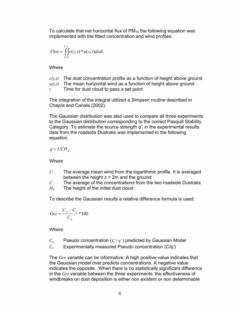
To calculate that net horizontal flux of PM10 the following equation was implemented with the fitted concentration and wind profiles:
∫ ∫∞
=T
dzdttzutzcFlux0 0
),(*),(
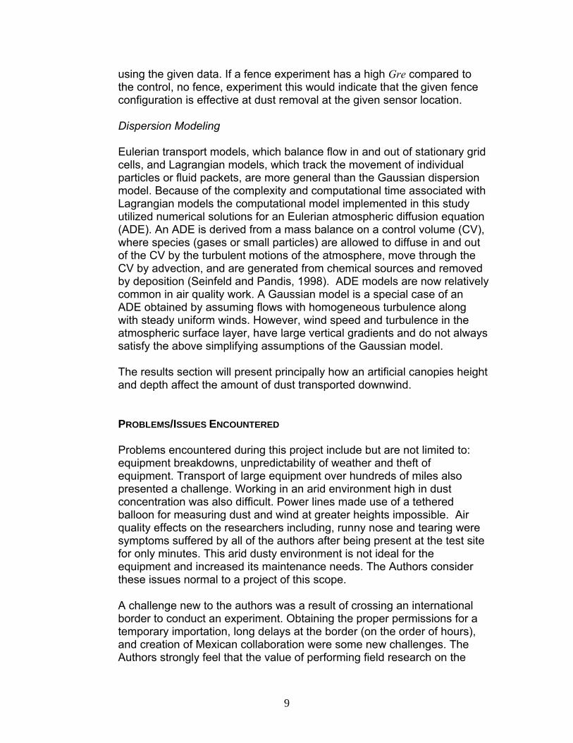
Where c(z,t) The dust concentration profile as a function of height above ground u(z,t) The mean horizontal wind as a function of height above ground t Time for dust cloud to pass a set point The integration of the integral utilized a Simpson routine described in Chapra and Canale (2002). The Gaussian distribution was also used to compare all three experiments to the Gaussian distribution corresponding to the correct Pasquill Stability Category. To estimate the source strength q’, in the experimental results data from the roadside Dustraks was implemented in the following equation.
dUCHq =' Where U The average mean wind from the logarithmic profile. It is averaged
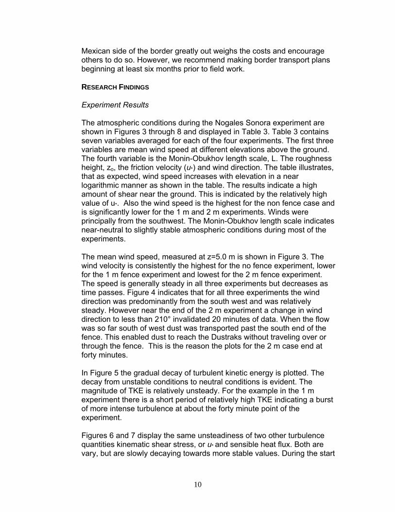
between the height z = 2m and the ground C The average of the concentrations from the two roadside Dustraks Hd The height of the initial dust cloud To describe the Gaussian results a relative difference formula is used:
100*g
eg
CCC
Gre−
=
Where Cg Pseudo concentration ( ) predicted by Gaussian Model '/ qCCe Experimentally measured Pseudo concentration (C/q’) The Gre variable can be informative. A high positive value indicates that the Gaussian model over predicts concentrations. A negative value indicates the opposite. When there is no statistically significant difference in the Gre variable between the three experiments, the effectiveness of windbreaks on dust deposition is either non existent or non determinable
8
using the given data. If a fence experiment has a high Gre compared to the control, no fence, experiment this would indicate that the given fence configuration is effective at dust removal at the given sensor location. Dispersion Modeling Eulerian transport models, which balance flow in and out of stationary grid cells, and Lagrangian models, which track the movement of individual particles or fluid packets, are more general than the Gaussian dispersion model. Because of the complexity and computational time associated with Lagrangian models the computational model implemented in this study utilized numerical solutions for an Eulerian atmospheric diffusion equation (ADE). An ADE is derived from a mass balance on a control volume (CV), where species (gases or small particles) are allowed to diffuse in and out of the CV by the turbulent motions of the atmosphere, move through the CV by advection, and are generated from chemical sources and removed by deposition (Seinfeld and Pandis, 1998). ADE models are now relatively common in air quality work. A Gaussian model is a special case of an ADE obtained by assuming flows with homogeneous turbulence along with steady uniform winds. However, wind speed and turbulence in the atmospheric surface layer, have large vertical gradients and do not always satisfy the above simplifying assumptions of the Gaussian model. The results section will present principally how an artificial canopies height and depth affect the amount of dust transported downwind.
PROBLEMS/ISSUES ENCOUNTERED
Problems encountered during this project include but are not limited to: equipment breakdowns, unpredictability of weather and theft of equipment. Transport of large equipment over hundreds of miles also presented a challenge. Working in an arid environment high in dust concentration was also difficult. Power lines made use of a tethered balloon for measuring dust and wind at greater heights impossible. Air quality effects on the researchers including, runny nose and tearing were symptoms suffered by all of the authors after being present at the test site for only minutes. This arid dusty environment is not ideal for the equipment and increased its maintenance needs. The Authors consider these issues normal to a project of this scope.
A challenge new to the authors was a result of crossing an international border to conduct an experiment. Obtaining the proper permissions for a temporary importation, long delays at the border (on the order of hours), and creation of Mexican collaboration were some new challenges. The Authors strongly feel that the value of performing field research on the
9
Mexican side of the border greatly out weighs the costs and encourage others to do so. However, we recommend making border transport plans beginning at least six months prior to field work.
RESEARCH FINDINGS
Experiment Results
The atmospheric conditions during the Nogales Sonora experiment are shown in Figures 3 through 8 and displayed in Table 3. Table 3 contains seven variables averaged for each of the four experiments. The first three variables are mean wind speed at different elevations above the ground. The fourth variable is the Monin-Obukhov length scale, L. The roughness height, zo, the friction velocity (u*) and wind direction. The table illustrates, that as expected, wind speed increases with elevation in a near logarithmic manner as shown in the table. The results indicate a high amount of shear near the ground. This is indicated by the relatively high value of u*. Also the wind speed is the highest for the non fence case and is significantly lower for the 1 m and 2 m experiments. Winds were principally from the southwest. The Monin-Obukhov length scale indicates near-neutral to slightly stable atmospheric conditions during most of the experiments.
The mean wind speed, measured at z=5.0 m is shown in Figure 3. The wind velocity is consistently the highest for the no fence experiment, lower for the 1 m fence experiment and lowest for the 2 m fence experiment. The speed is generally steady in all three experiments but decreases as time passes. Figure 4 indicates that for all three experiments the wind direction was predominantly from the south west and was relatively steady. However near the end of the 2 m experiment a change in wind direction to less than 210° invalidated 20 minutes of data. When the flow was so far south of west dust was transported past the south end of the fence. This enabled dust to reach the Dustraks without traveling over or through the fence. This is the reason the plots for the 2 m case end at forty minutes.
In Figure 5 the gradual decay of turbulent kinetic energy is plotted. The decay from unstable conditions to neutral conditions is evident. The magnitude of TKE is relatively unsteady. For the example in the 1 m experiment there is a short period of relatively high TKE indicating a burst of more intense turbulence at about the forty minute point of the experiment.
Figures 6 and 7 display the same unsteadiness of two other turbulence quantities kinematic shear stress, or u* and sensible heat flux. Both are vary, but are slowly decaying towards more stable values. During the start
10
of the no fence experiment, small positive values of heat flux are measured. Positive values of kinematic sensible heat flux generally indicate an unstable boundary layer. However the small magnitude of the heat flux indicates a near neutral boundary layer. The values during the majority of the experiment, namely moderate values for u* and small negative values for kinematic heat flux are also indicative of a neutral boundary layer.
Figure 8 confirms the previous conclusions. The Monin-Obukhov length scale, L, is a measure of buoyancy driven turbulence in the atmosphere. The large positive values indicate an atmosphere with negligible buoyancy generated turbulence. At the start of the no fence example, the L scale is negative, which generally indicates a unstable atmosphere. However the magnitude is so large that this length scale indicates a stable boundary layer. This parallels the heat flux conclusion for the no fence experiment in Figure 7 because the Monin-Obukhov length is a function of kinematic shear stress.
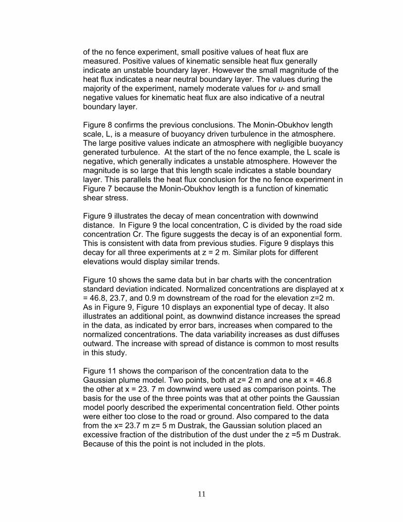
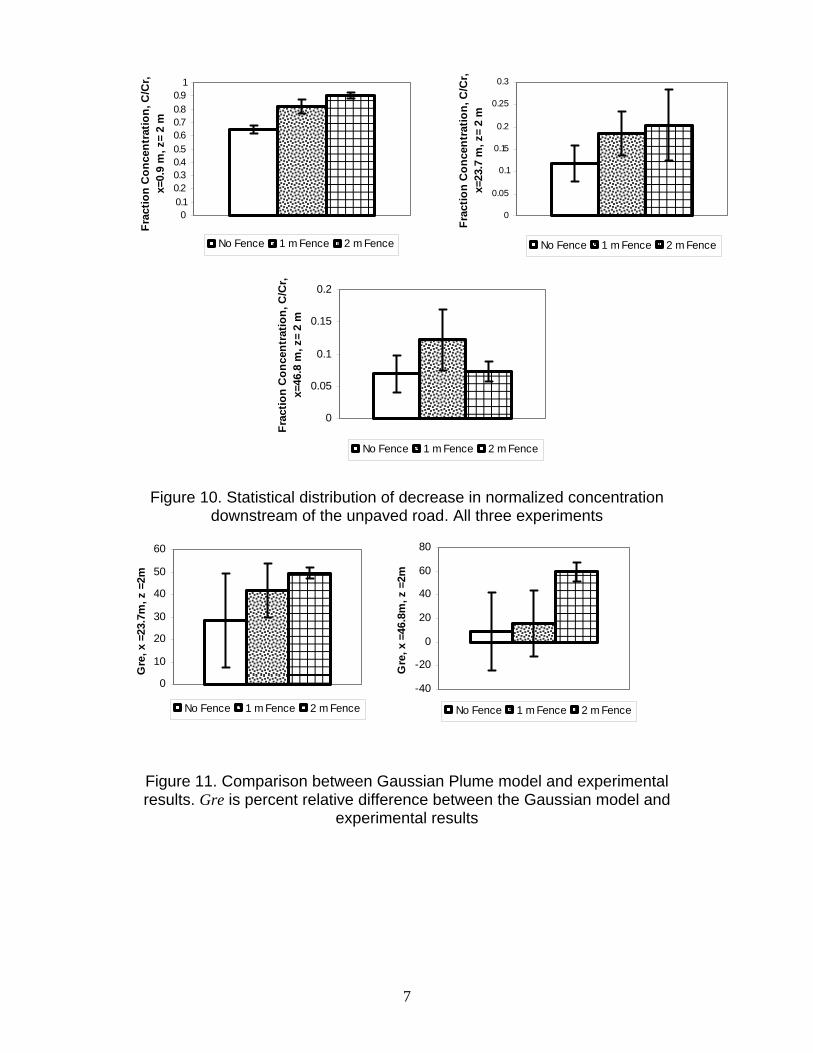
Figure 9 illustrates the decay of mean concentration with downwind distance. In Figure 9 the local concentration, C is divided by the road side concentration Cr. The figure suggests the decay is of an exponential form. This is consistent with data from previous studies. Figure 9 displays this decay for all three experiments at z = 2 m. Similar plots for different elevations would display similar trends.
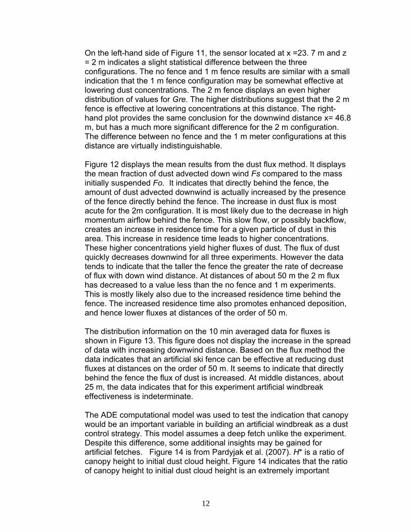
Figure 10 shows the same data but in bar charts with the concentration standard deviation indicated. Normalized concentrations are displayed at x = 46.8, 23.7, and 0.9 m downstream of the road for the elevation z=2 m. As in Figure 9, Figure 10 displays an exponential type of decay. It also illustrates an additional point, as downwind distance increases the spread in the data, as indicated by error bars, increases when compared to the normalized concentrations. The data variability increases as dust diffuses outward. The increase with spread of distance is common to most results in this study.
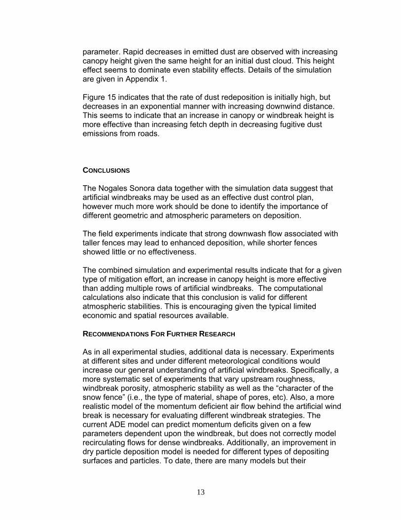
Figure 11 shows the comparison of the concentration data to the Gaussian plume model. Two points, both at z= 2 m and one at x = 46.8 the other at x = 23. 7 m downwind were used as comparison points. The basis for the use of the three points was that at other points the Gaussian model poorly described the experimental concentration field. Other points were either too close to the road or ground. Also compared to the data from the x= 23.7 m z= 5 m Dustrak, the Gaussian solution placed an excessive fraction of the distribution of the dust under the z =5 m Dustrak. Because of this the point is not included in the plots.
11
On the left-hand side of Figure 11, the sensor located at x =23. 7 m and z = 2 m indicates a slight statistical difference between the three configurations. The no fence and 1 m fence results are similar with a small indication that the 1 m fence configuration may be somewhat effective at lowering dust concentrations. The 2 m fence displays an even higher distribution of values for Gre. The higher distributions suggest that the 2 m fence is effective at lowering concentrations at this distance. The right-hand plot provides the same conclusion for the downwind distance x= 46.8 m, but has a much more significant difference for the 2 m configuration. The difference between no fence and the 1 m meter configurations at this distance are virtually indistinguishable.
Figure 12 displays the mean results from the dust flux method. It displays the mean fraction of dust advected down wind Fs compared to the mass initially suspended Fo. It indicates that directly behind the fence, the amount of dust advected downwind is actually increased by the presence of the fence directly behind the fence. The increase in dust flux is most acute for the 2m configuration. It is most likely due to the decrease in high momentum airflow behind the fence. This slow flow, or possibly backflow, creates an increase in residence time for a given particle of dust in this area. This increase in residence time leads to higher concentrations. These higher concentrations yield higher fluxes of dust. The flux of dust quickly decreases downwind for all three experiments. However the data tends to indicate that the taller the fence the greater the rate of decrease of flux with down wind distance. At distances of about 50 m the 2 m flux has decreased to a value less than the no fence and 1 m experiments. This is mostly likely also due to the increased residence time behind the fence. The increased residence time also promotes enhanced deposition, and hence lower fluxes at distances of the order of 50 m.
The distribution information on the 10 min averaged data for fluxes is shown in Figure 13. This figure does not display the increase in the spread of data with increasing downwind distance. Based on the flux method the data indicates that an artificial ski fence can be effective at reducing dust fluxes at distances on the order of 50 m. It seems to indicate that directly behind the fence the flux of dust is increased. At middle distances, about 25 m, the data indicates that for this experiment artificial windbreak effectiveness is indeterminate.
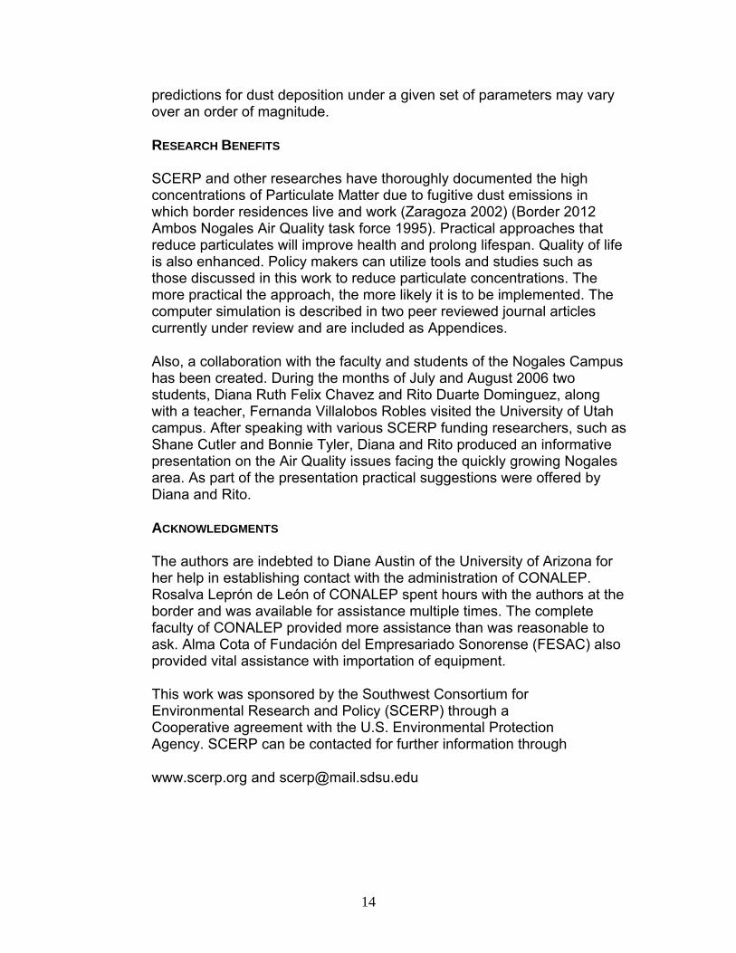
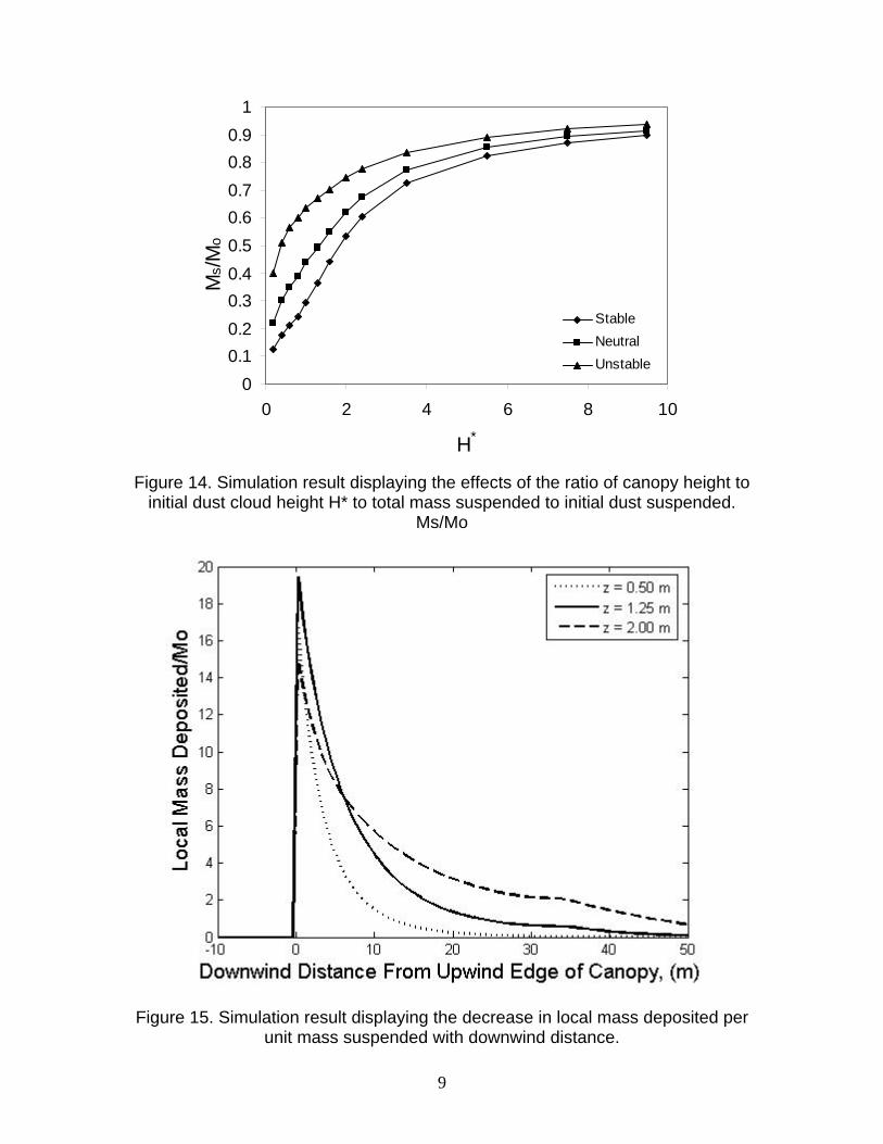
The ADE computational model was used to test the indication that canopy would be an important variable in building an artificial windbreak as a dust control strategy. This model assumes a deep fetch unlike the experiment. Despite this difference, some additional insights may be gained for artificial fetches. Figure 14 is from Pardyjak et al. (2007). H* is a ratio of canopy height to initial dust cloud height. Figure 14 indicates that the ratio of canopy height to initial dust cloud height is an extremely important
12
parameter. Rapid decreases in emitted dust are observed with increasing canopy height given the same height for an initial dust cloud. This height effect seems to dominate even stability effects. Details of the simulation are given in Appendix 1.
Figure 15 indicates that the rate of dust redeposition is initially high, but decreases in an exponential manner with increasing downwind distance. This seems to indicate that an increase in canopy or windbreak height is more effective than increasing fetch depth in decreasing fugitive dust emissions from roads.
CONCLUSIONS
The Nogales Sonora data together with the simulation data suggest that artificial windbreaks may be used as an effective dust control plan, however much more work should be done to identify the importance of different geometric and atmospheric parameters on deposition.
The field experiments indicate that strong downwash flow associated with taller fences may lead to enhanced deposition, while shorter fences showed little or no effectiveness.
The combined simulation and experimental results indicate that for a given type of mitigation effort, an increase in canopy height is more effective than adding multiple rows of artificial windbreaks. The computational calculations also indicate that this conclusion is valid for different atmospheric stabilities. This is encouraging given the typical limited economic and spatial resources available.
RECOMMENDATIONS FOR FURTHER RESEARCH
As in all experimental studies, additional data is necessary. Experiments at different sites and under different meteorological conditions would increase our general understanding of artificial windbreaks. Specifically, a more systematic set of experiments that vary upstream roughness, windbreak porosity, atmospheric stability as well as the “character of the snow fence” (i.e., the type of material, shape of pores, etc). Also, a more realistic model of the momentum deficient air flow behind the artificial wind break is necessary for evaluating different windbreak strategies. The current ADE model can predict momentum deficits given on a few parameters dependent upon the windbreak, but does not correctly model recirculating flows for dense windbreaks. Additionally, an improvement in dry particle deposition model is needed for different types of depositing surfaces and particles. To date, there are many models but their
13
predictions for dust deposition under a given set of parameters may vary over an order of magnitude.
RESEARCH BENEFITS
SCERP and other researches have thoroughly documented the high concentrations of Particulate Matter due to fugitive dust emissions in which border residences live and work (Zaragoza 2002) (Border 2012 Ambos Nogales Air Quality task force 1995). Practical approaches that reduce particulates will improve health and prolong lifespan. Quality of life is also enhanced. Policy makers can utilize tools and studies such as those discussed in this work to reduce particulate concentrations. The more practical the approach, the more likely it is to be implemented. The computer simulation is described in two peer reviewed journal articles currently under review and are included as Appendices.
Also, a collaboration with the faculty and students of the Nogales Campus has been created. During the months of July and August 2006 two students, Diana Ruth Felix Chavez and Rito Duarte Dominguez, along with a teacher, Fernanda Villalobos Robles visited the University of Utah campus. After speaking with various SCERP funding researchers, such as Shane Cutler and Bonnie Tyler, Diana and Rito produced an informative presentation on the Air Quality issues facing the quickly growing Nogales area. As part of the presentation practical suggestions were offered by Diana and Rito.
ACKNOWLEDGMENTS
The authors are indebted to Diane Austin of the University of Arizona for her help in establishing contact with the administration of CONALEP. Rosalva Leprón de León of CONALEP spent hours with the authors at the border and was available for assistance multiple times. The complete faculty of CONALEP provided more assistance than was reasonable to ask. Alma Cota of Fundación del Empresariado Sonorense (FESAC) also provided vital assistance with importation of equipment. This work was sponsored by the Southwest Consortium for Environmental Research and Policy (SCERP) through a Cooperative agreement with the U.S. Environmental Protection Agency. SCERP can be contacted for further information through
www.scerp.org and [email protected]
14
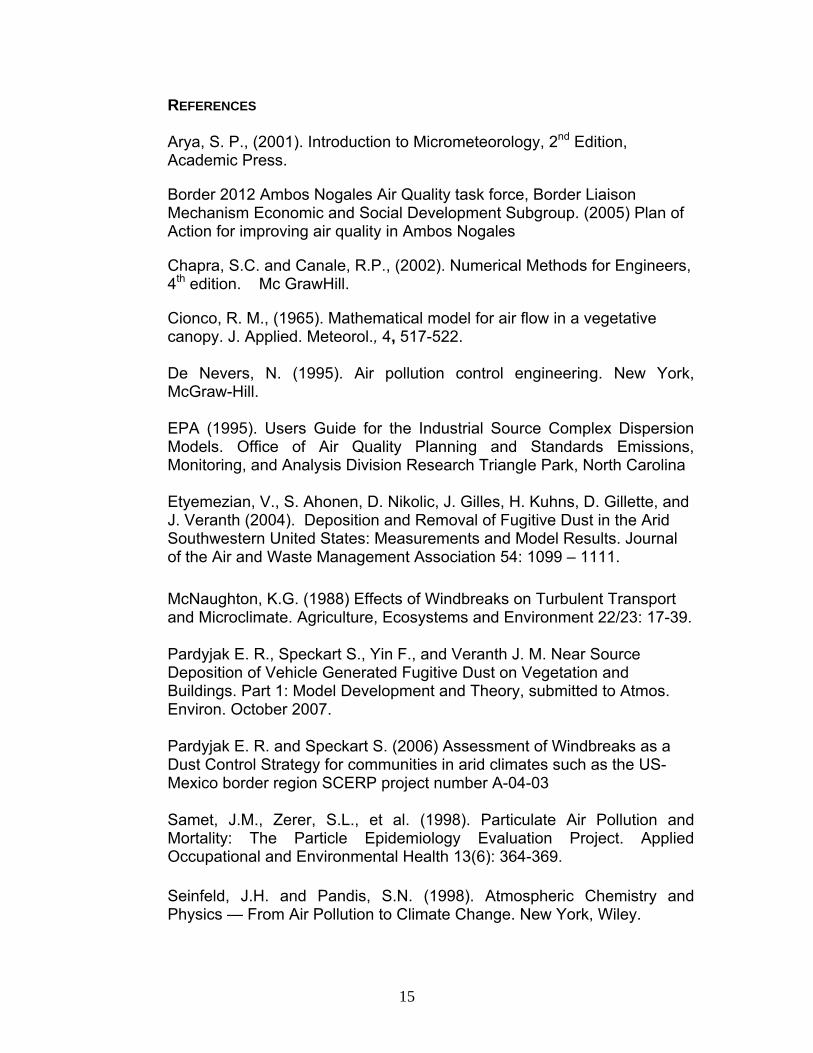
REFERENCES
Arya, S. P., (2001). Introduction to Micrometeorology, 2nd Edition, Academic Press.
Border 2012 Ambos Nogales Air Quality task force, Border Liaison Mechanism Economic and Social Development Subgroup. (2005) Plan of Action for improving air quality in Ambos Nogales
Chapra, S.C. and Canale, R.P., (2002). Numerical Methods for Engineers, 4th edition. Mc GrawHill.
Cionco, R. M., (1965). Mathematical model for air flow in a vegetative canopy. J. Applied. Meteorol., 4, 517-522. De Nevers, N. (1995). Air pollution control engineering. New York, McGraw-Hill. EPA (1995). Users Guide for the Industrial Source Complex Dispersion Models. Office of Air Quality Planning and Standards Emissions, Monitoring, and Analysis Division Research Triangle Park, North Carolina Etyemezian, V., S. Ahonen, D. Nikolic, J. Gilles, H. Kuhns, D. Gillette, and J. Veranth (2004). Deposition and Removal of Fugitive Dust in the Arid Southwestern United States: Measurements and Model Results. Journal of the Air and Waste Management Association 54: 1099 – 1111. McNaughton, K.G. (1988) Effects of Windbreaks on Turbulent Transport and Microclimate. Agriculture, Ecosystems and Environment 22/23: 17-39.
Pardyjak E. R., Speckart S., Yin F., and Veranth J. M. Near Source Deposition of Vehicle Generated Fugitive Dust on Vegetation and Buildings. Part 1: Model Development and Theory, submitted to Atmos. Environ. October 2007.
Pardyjak E. R. and Speckart S. (2006) Assessment of Windbreaks as a Dust Control Strategy for communities in arid climates such as the US-Mexico border region SCERP project number A-04-03
Samet, J.M., Zerer, S.L., et al. (1998). Particulate Air Pollution and Mortality: The Particle Epidemiology Evaluation Project. Applied Occupational and Environmental Health 13(6): 364-369. Seinfeld, J.H. and Pandis, S.N. (1998). Atmospheric Chemistry and Physics — From Air Pollution to Climate Change. New York, Wiley.
15
Stull R. (1998) An Introduction to Boundary Layer Meteorology. Kluwer Academic Publishers
Turner, D. B. (1970). Workbook of atmospheric dispersion estimates. Washington, U.S. Government Printing Office. Wilczak, J. M., Oncley, S. P., and Sage, S. A. (2001). Sonic Anemometer Tilt Correction Algorithms, Boundary-Layer Meteorol. 99, 127–150. Veranth, J. M., Seshadri, G. and Pardyjak, E. (2003). Vehicle-generated fugitive dust transport: Analytic models and field study. Atmospheric Environment 37(16): 2295-2303. Veranth, J. M., Speckart S., Yin F., Etyemezian V. and Pardyjak, E. Near-source deposition of Vehicle-Generated Fugitive Dust on Vegetation and Buildings. Part 2. Field Measurements and Model Validation. Submitted to Atmos. Environ. October 2007. Zaragoza, Xavier (2002) “It’s all up in the air.” The Daily Dispatch (April 27-28)
16
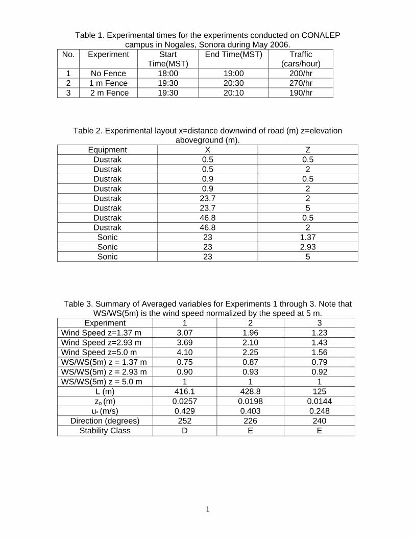
Table 1. Experimental times for the experiments conducted on CONALEP campus in Nogales, Sonora during May 2006.
No. Experiment Start Time(MST)
End Time(MST) Traffic (cars/hour)
1 No Fence 18:00 19:00 200/hr 2 1 m Fence 19:30 20:30 270/hr 3 2 m Fence 19:30 20:10 190/hr
Table 2. Experimental layout x=distance downwind of road (m) z=elevation aboveground (m).
Equipment X Z Dustrak 0.5 0.5 Dustrak 0.5 2 Dustrak 0.9 0.5 Dustrak 0.9 2 Dustrak 23.7 2 Dustrak 23.7 5 Dustrak 46.8 0.5 Dustrak 46.8 2 Sonic 23 1.37 Sonic 23 2.93 Sonic 23 5
Table 3. Summary of Averaged variables for Experiments 1 through 3. Note that WS/WS(5m) is the wind speed normalized by the speed at 5 m.
Experiment 1 2 3 Wind Speed z=1.37 m 3.07 1.96 1.23 Wind Speed z=2.93 m 3.69 2.10 1.43 Wind Speed z=5.0 m 4.10 2.25 1.56 WS/WS(5m) z = 1.37 m 0.75 0.87 0.79 WS/WS(5m) z = 2.93 m 0.90 0.93 0.92 WS/WS(5m) z = 5.0 m 1 1 1
L (m) 416.1 428.8 125 zo (m) 0.0257 0.0198 0.0144
u* (m/s) 0.429 0.403 0.248 Direction (degrees) 252 226 240
Stability Class D E E
1
(a)
)(zU
x
H Reattachment point
Downward velocity
)(c
)(b
Displaced Profile
Quiet Zone
Mixing Zone Re-equilibration Zone
Bleed Flow
x
Enhanced Deposition
Enhanced Deposition
)(zU
H
Figure 1. Physics of Dust Removal from (a) deep vegetative canopy, (b) high
solidity windbreak and (c) low-solidity wind break.
2
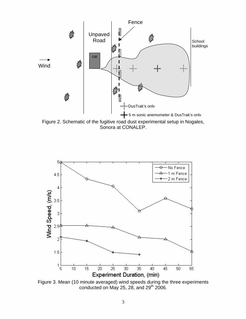
Figure 2. Schematic of the fugitive road dust experimental setup in Nogales,
Sonora at CONALEP.
Unpaved Road
Fence
Wind
car
DusTrak’s only
School buildings
5 m sonic anemometer & DusTrak’s only
Figure 3. Mean (10 minute averaged) wind speeds during the three experiments
conducted on May 25, 28, and 29th 2006.
3
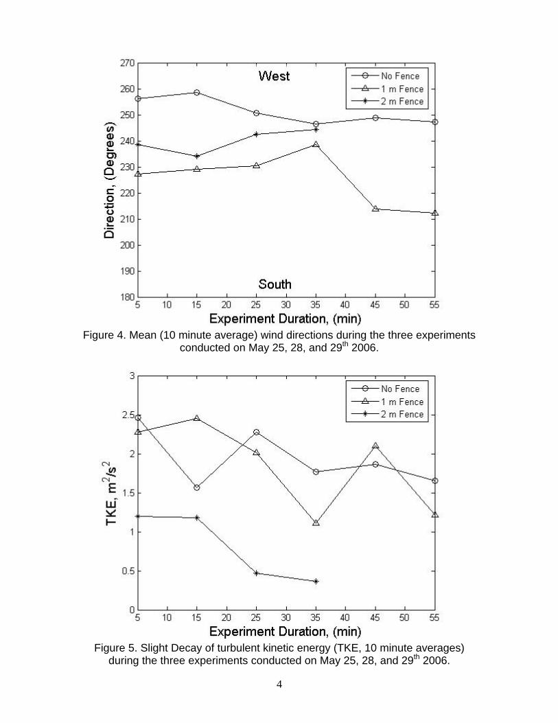
Figure 4. Mean (10 minute average) wind directions during the three experiments
conducted on May 25, 28, and 29th 2006.
Figure 5. Slight Decay of turbulent kinetic energy (TKE, 10 minute averages)
during the three experiments conducted on May 25, 28, and 29th 2006.
4
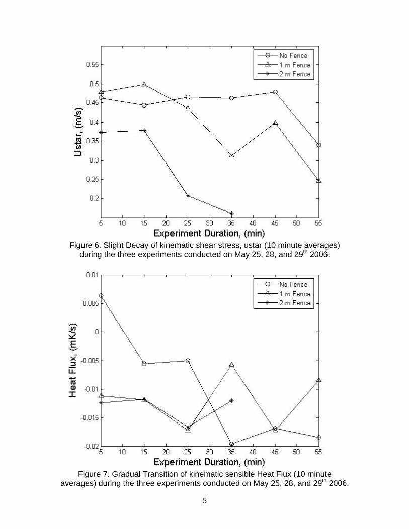
Figure 6. Slight Decay of kinematic shear stress, ustar (10 minute averages)
during the three experiments conducted on May 25, 28, and 29th 2006.
Figure 7. Gradual Transition of kinematic sensible Heat Flux (10 minute
averages) during the three experiments conducted on May 25, 28, and 29th 2006.
5
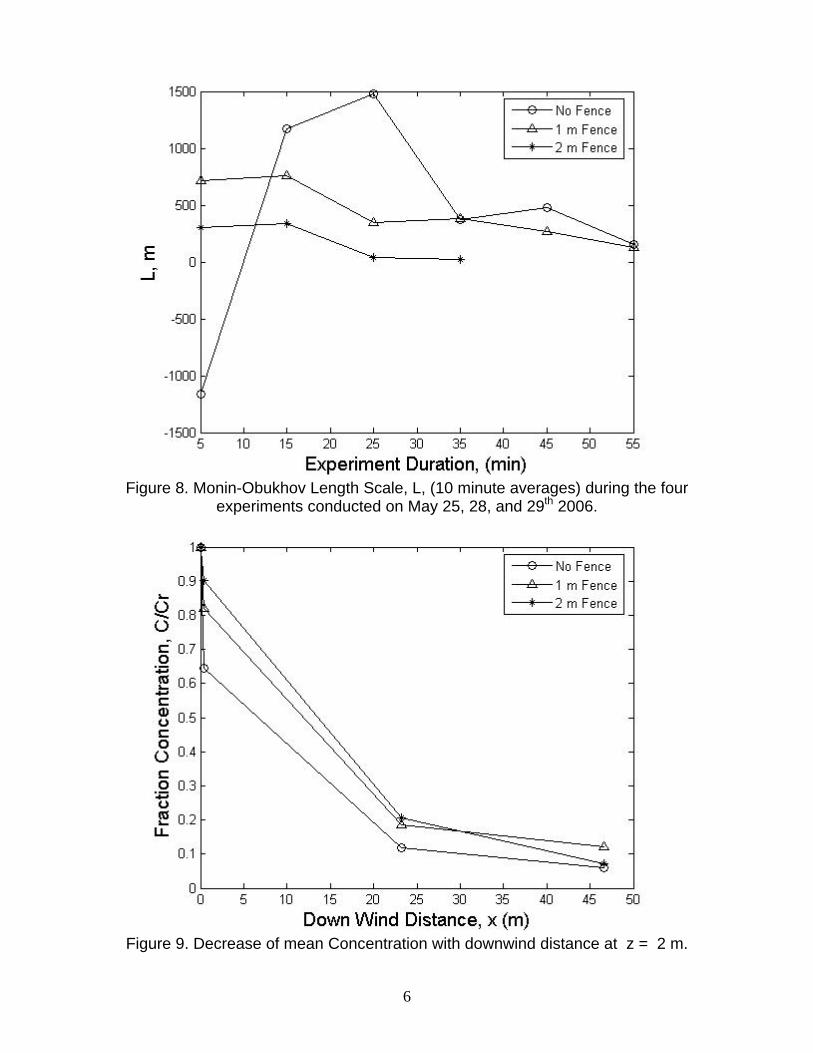
Figure 8. Monin-Obukhov Length Scale, L, (10 minute averages) during the four
experiments conducted on May 25, 28, and 29th 2006.
Figure 9. Decrease of mean Concentration with downwind distance at z = 2 m.
6
0
0.05
0.1
0.15
0.2
0.25
0.3
Frac
tion
Con
cent
ratio
n, C
/Cr,
x=23
.7 m
, z=
2 m
No Fence 1 m Fence 2 m Fence
0
0.05
0.1
0.15
0.2Fr
actio
n C
once
ntra
tion,
C/C
r, x=
46.8
m, z
= 2
m
No Fence 1 m Fence 2 m Fence
00.10.20.30.40.50.60.70.80.9
1
Frac
tion
Con
cent
ratio
n, C
/Cr,
x=0.
9 m
, z=
2 m
No Fence 1 m Fence 2 m Fence
Figure 10. Statistical distribution of decrease in normalized concentration
downstream of the unpaved road. All three experiments
0
10
20
30
40
50
60
Gre
, x =
23.7
m, z
=2m
No Fence 1 m Fence 2 m Fence
-40
-20
0
20
40
60
80
Gre
, x =
46.8
m, z
=2m
No Fence 1 m Fence 2 m Fence
Figure 11. Comparison between Gau sian Plume model and experimental sresults. Gre is percent relative difference between the Gaussian model and
experimental results
7
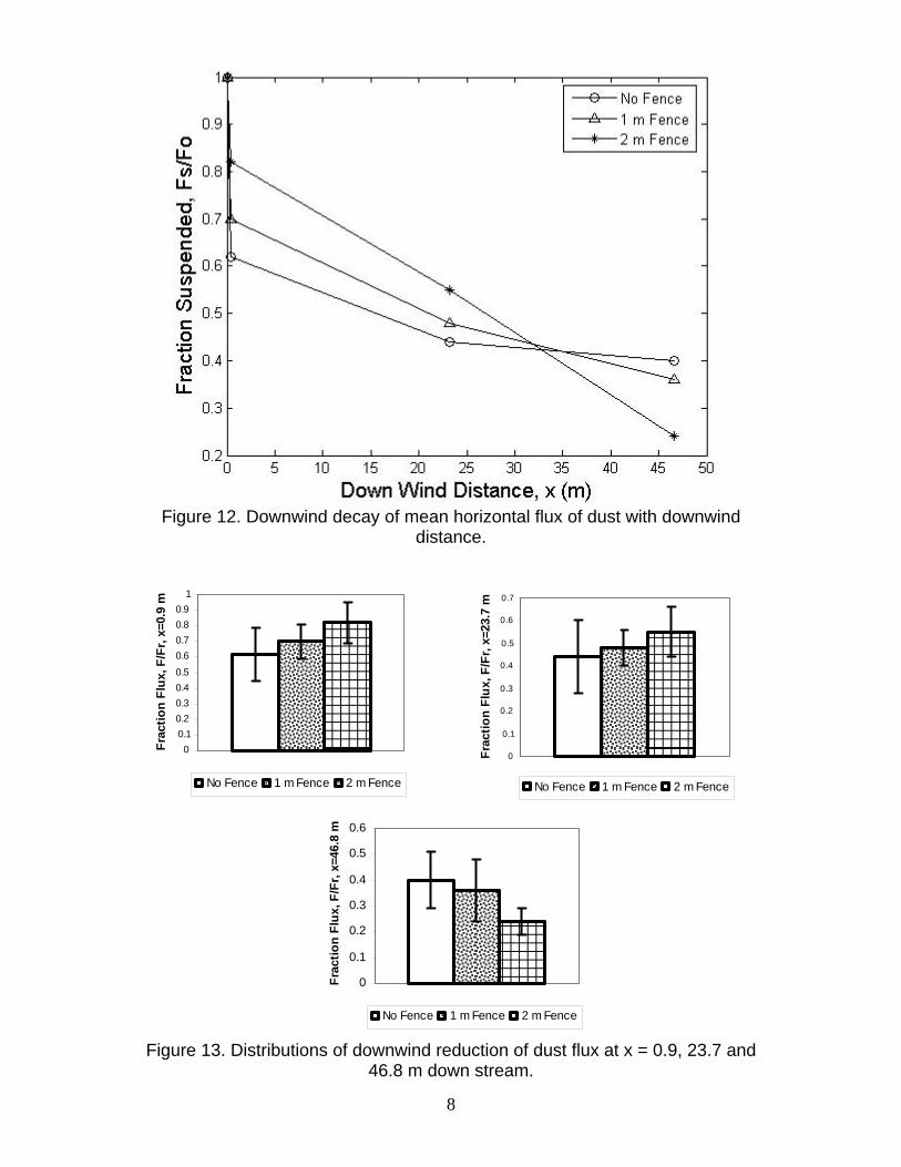
Figure 12. Downwind decay of mean horizontal flux of dust with downwind
distance.
0
0.1
0.2
0.3
0.4
0.5
0.6
0.7
Frac
tion
Flux
, F/F
r, x=
23.7
m
No Fence 1 m Fence 2 m Fence
0
0.1
0.2
0.3
0.4
0.5
0.6
Frac
tion
Flux
, F/F
r, x=
46.8
m
No Fence 1 m Fence 2 m Fence
00.10.20.30.40.5
0.60.70.80.9
1
Frac
tion
Flux
, F/F
r, x=
0.9
m
No Fence 1 m Fence 2 m Fence
Figure 13. Distributions of downwind reduction of dust flux at x = 0.9, 23.7 and 46.8 m down stream.
8
00.10.20.30.40.50.60.70.80.9
1
0 2 4 6 8 1
H*
Ms/M
o
0
StableNeutralUnstable
Figure 14. Simulation result displaying the effects of the ratio of canopy height to
initial dust cloud height H* to total mass suspended to initial dust suspended. Ms/Mo
Figure 15. Simulation result displaying the decrease in local mass deposited per unit mass suspended with downwind distance.
9

APPENDIX 1
1
Near Source Deposition of Vehicle Generated Fugitive Dust on Vegetation and Buildings, Part I: Model Development and Theory
E.R. Pardyjak1, S.O. Speckart1, F. Yin2 and J. M. Veranth3
1. Department of Mechanical Engineering, University of Utah, Salt Lake City, Utah
2. Department of Chemical Engineering, University of Utah, Salt Lake City, Utah
3. Department of Pharmacology and Toxicology, University of Utah, Salt Lake City, Utah
Manuscript for submission to Atmospheric Environment
October 17, 2007
Corresponding Author Eric R. Pardyjak University of Utah Room 2110 Salt Lake City, UT 84112 Tel: 801-585-6414 Fax: 801-585-0039 [email protected]
2

Abstract
This paper describes the development of a simple quasi-2D Eulerian atmospheric dispersion
model that accounts for dry deposition of fugitive dust onto vegetation and buildings. The focus
of this work is on the effects of atmospheric surface layer parameterizations on deposition in the
“impact zone” near unpaved roads where horizontal advection of a dust cloud through roughness
is important. A wind model for computing average and turbulent wind fields is presented for
flow within and above a roughness canopy. The canopy model has been developed to capture the
most essential transport and deposition physics while minimizing the number of difficult to
obtain input parameters. The deposition model is based on a bulk sink term in the transport
equation that lumps the various dry deposition physical process. Wind field, turbulence and
deposition results are presented for a range atmospheric stabilities and roughnesses. The canopy
model produces results in which deposition within a canopy is enhanced under certain initial,
atmospheric and roughness conditions, while under other conditions much less deposition
occurs. The primary limitation of the model is the ability to accurately determine (typically using
experimental data) the vegetative deposition parameter (clearance frequency). To understand the
clearance frequency better, a dimensionless parameter called the transport effectiveness is
identified and the limiting cases discussed. In general, the model captures the essential physics of
near source dust transport and provides a tool that can efficiently simulate site-specific
conditions in practical situations.
Keywords: fugitive dust; near-source deposition; roughness; vegetation; vehicle generated dust
3
1. Introduction
Vehicle generated fugitive dust is the uncontrolled emission of particulate matter associated with
vehicles driving over unpaved roads. These emissions are particularly important in populated
arid regions with many kilometers of unpaved roads such as the cities along the U.S./Mexico
border. The amount of fugitive dust that is transported long distances from these sources can
have a great impact on health (Davidson et al., 2005) and visibility (Watson and Chow, 1994). A
number of abatement strategies exist including the application of liquids onto unpaved roads
(Harley et al., 1989) but many options are uneconomical or ineffective in arid climates with
extensive rural roads. It has been proposed that another strategy for reducing these emissions is
to utilize natural vegetation and windbreaks (Pace, 2005). In addition, studies indicate (Watson
and Chow, 2000), that current EPA emission factors over predict long range transport. One
hypothesis for this overestimate is that the emission factor model does not account for particle
removal by vegetation or other roughness elements near the source. In order to understand the
net emissions from unpaved roads, it is necessary to quantify the amount of dust that is deposited
near the source before the dust cloud is well mixed.
There have been a wide range of studies focusing on measuring and modeling the dry deposition
of particles onto vegetation and other surface roughness (for reviews see e.g., Nicholson, 1988;
Sehmel, 1980; Seinfeld and Pandis, 1998). Dry deposition of particles in the atmospheric
boundary layer is governed by the turbulent flow characteristics, the physical and chemical
properties of the material being deposited and the nature of the surface (Seinfeld and Pandis,
1998). Deposition of particles onto surfaces occurs primarily by the following mechanisms:
impaction, Brownian diffusion, interception, gravitational settling (or sedimentation) and
phoretic (diffusiophoresis, thermophoresis, electrophoresis) precipitation (Nicholson, 1988).
4
Impaction and gravitational settling occur when particles cross streamlines as a result of particle
inertia. In Brownian diffusion, particles cross streamlines as a result of molecular bombardment
of air molecules on particles. Interception occurs when the radius of the particle is large
compared to the particles distance to the surface of the intercepting element (e.g. leaf). Much of
the existing literature related to particle deposition onto roughness elements (Chamberlain, 1975;
Raupach et al., 2001; Slinn, 1982) considers transport far downwind of the source where
concentrations are relatively uniform with height and the horizontal surface is considered a sink.
This type of problem is typically modeled using a deposition velocity formulation that considers
different physical processes as a resistance network analogy (Seinfeld and Pandis, 1998).
Deposition near the source, or more specifically in the “impact zone”, however is less well
understood. Figure 1 illustrates the limiting cases for dust transport (adapted from Etyemezian et
al., 2004) near an unpaved road. The limiting cases include the impact, transition and far
downwind zones. In the impact zone, the height of the dust cloud is of the same order of
magnitude as the height of the vegetation, terrain irregularities, fences, buildings, or other
roughness elements. The concentration of dust is highest near the ground. In the transition zone,
the cloud is much taller and vertical concentration gradients are lower compared to the impact
zone. In the far downwind zone, the dust is fairly uniformly distributed throughout the height of
the atmospheric surface layer, except very near the ground. This study focuses on dust removal
very close to the road where the dust cloud is in the impact zone.
Etyemezian et al. (2004) studied the behavior of a dust cloud downwind of a dirt road at Ft.
Bliss, near El Paso, Texas U.S.A. during late spring 2002. The test site consisted of small dunes
5
with widely spaced desert shrub vegetation (aerodynamic roughness of ~0.001-0.01 m) and
neutral to unstable atmospheric conditions. The field data were compared to a line source
Gaussian plume model in a near-road dust simulation. The measurements indicated that the loss
of PM10 (particulate matter with an aerodynamic diameter of 10μm or less) within 100 m
downwind of the source was within measurement uncertainty (less than ~10%). The EPA
Industrial Source Code version 3 (ISC3), a Gaussian based model, indicated the loss of PM10 to
be less than 5%. Etyemezian et al. (2004) concluded that the EPA ISC3 model is a simplistic but
reasonable first approximation for this problem.
Veranth et al. (2003) studied a similar dust dispersion problem downstream of a dirt road in
Utah’s west desert at The U.S. Army Dugway Proving Grounds (DPG). They investigated the
loss of PM10 through a mock array of buildings downwind of an unpaved road under stable
atmospheric conditions. The downstream surface roughness was created using shipping
containers (2.5 m high, 2.4 m deep and 12.2 m long) in a rectangular 10 × 12 array. The data
revealed a removal of 85% for PM10 within the first 100 m downwind. Etyemezian et al. (2004)
also used the Gaussian based model to analyze this experiment assuming very stable conditions
and a much larger roughness height, (0.71 m) than for the Ft. Bliss study. The Gaussian model
predicted only 30% removal for the DPG experiment. We hypothesize that the discrepancy
between the Ft. Bliss and DPG data is a result of the Gaussian model’s inability (due to the
model’s basic assumptions being violated) to capture the complex physics associated with flow
through buildings capped by a stable inversion. The discrepancy between the two problems has
motivated the authors of the present paper to develop a simple model that more accurately
captures the physics associated with dust transport through roughness elements subject to
different atmospheric stabilities.
6
In order to develop a practical model for deposition, the wind and turbulence field through the
roughness elements must be carefully modeled. In recent years, a great deal of progress has been
made regarding understanding turbulent flow through and above obstacles in the atmospheric
surface layer. In particular, flows associated with vegetation (Finnigan, 2000; Raupach and
Thom, 1981) and buildings (Belcher, 2005; Britter and Hanna, 2003) have received much
attention. While the details of the fundamental processes that govern the flow within vegetative
and building canopies are quite different, some of the bulk properties can be modeled similarly.
For example, the results of (Macdonald, 2000) for mean flow and turbulence parameterizations
for groups of buildings, which is based on the vegetative canopy model, yield a good comparison
to experimental results. One of the goals of the present work was to build on this previous
canopy research to develop a simple model for the mean velocity and turbulence that can be
easily applied to fugitive road dust problems in the impact zone. This has been done using a
simple two dimensional Eulerian atmospheric diffusion equation model described below. An
attempt is made to minimize the number of difficult to obtain input parameters while retaining
import physical processes. For example, if the geometry of the problem is known (i.e. height of
the canopy, type of canopy, road width, distance from road to the roughness and typical vehicle
height) and the deposition coefficient (described in detail in section 2.2) can be estimated, the
model can implemented if the upstream wind speed is known at a reference height along with an
estimate for atmospheric stability. Other wind (Harman and Finnigan, 2007; Macdonald, 2000;
Poggi et al., 2004) and deposition models (Aylor and Flesch, 2001; Raupach et al., 2001; Slinn,
1982) require detailed knowledge of the roughness elements. Below, we present the
development of the model and the general performance of the model. In the companion paper
(Veranth et al., 2007), the model is validated with full scale experimental data.
7
2. Methods
2.1. Atmospheric Diffusion Model
Eulerian transport models, which balance flow in and out of stationary grid cells, and Lagrangian
models, which track the movement of individual particles are more general than Gaussian
dispersion models because they are able to more easily incorporate complex physical processes
(Ramaswami et al., 2005; Seinfeld and Pandis, 1998). Because of the complexity and
computational time associated with Lagrangian dispersion models, this study utilized numerical
solutions to a quasi-two dimensional Eulerian atmospheric diffusion equation (ADE). For this
work, an ADE has been derived from a mass balance on a control volume (CV) in which small
particles are allowed to transport in and out of the CV by mean advection and turbulent motions
of the atmosphere. Molecular diffusion is assumed negligible compared to turbulent diffusion
and turbulent diffusion is modeled using K-Theory; additionally, source (dust generated by
vehicular motion) and sink (deposition) terms may be defined in each cell following Seinfeld and
Pandis (1998). ADE models are now relatively common in air quality work. A Gaussian model
is a special case of the solution of an ADE obtained for flows with homogeneous turbulence
along with steady uniform winds (Seinfeld and Pandis, 1998). However, wind speed and
turbulence in the rough wall atmospheric surface layer, have complex gradients that do not
always satisfy the simplifying assumptions of the Gaussian model.
The 2D ADE used in this study is modified to consider dust deposition on a rough walled
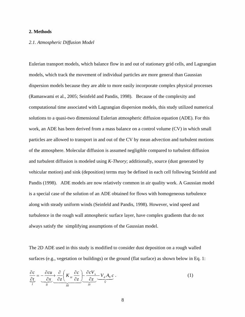
surfaces (e.g., vegetation or buildings) or the ground (flat surface) as shown below in Eq. 1:
{ 4342132144 344 21321 V
Vd
IV
s
III
zz
III
cAVz
cVzcK
zxcu
tc
−∂
∂−⎟⎠⎞
⎜⎝⎛
∂∂
∂∂
+∂∂
−=∂∂ . (1)
8
In Eq. 1, c is the concentration of dust in (mg m-3), u is the local streamwise velocity in m s-1, Kzz
is the vertical turbulent mixing coefficient in m2 s-1, Vs is the gravitational settling velocity in m
s-1, Vd is the horizontal deposition velocity onto the roughness elements in m-s-1 and Av is the
effective deposition area per volume of space m2 m-3 and includes the ground surface. Equation 1
is an ensemble averaged equation; hence c and u are ensemble averaged quantities. The physical
interpretation of the terms is as follows: term I is the local accumulation of dust within a CV;
term II is the advection of dust by the mean flow; term III represents the turbulent diffusion in
the vertical direction; term IV is the gravitational setting, and term V represents the total practical
deposition sink to the vegetation. Term V does not explicitly differentiate all of the different
mechanisms associated with deposition onto roughness elements, but rather bulks the processes
together into one lumped term. As noted above, this is a “quasi” 2D model because the velocity
field is specified by a canopy profile model that is described in following sections, not by a set of
prognostic equations. While the canopy model described herein does not explicitly resolve the
geometry of the vegetation, it does include the effects of the vegetation on the momentum field.
2.2. Deposition model
Specifying the effective deposition area per unit volume can be quite difficult for complex
vegetative or anthropogenic surfaces, and the numeric value for V
VA
d depends on the assumptions
made regarding the surface area. However theV product can be directly obtained from
measurements of mass deposited per time and aerosol concentration. This combined term is
treated as a single modeled sink parameter that is constant with height up to the top of the
canopy (except at the bottom cell where it includes the ground surface) and adjusted to match
experimental data (Veranth et al., 2007). Since no vegetative deposition occurs above the
canopy, V above the canopy.
Vd A
0=AVd
9
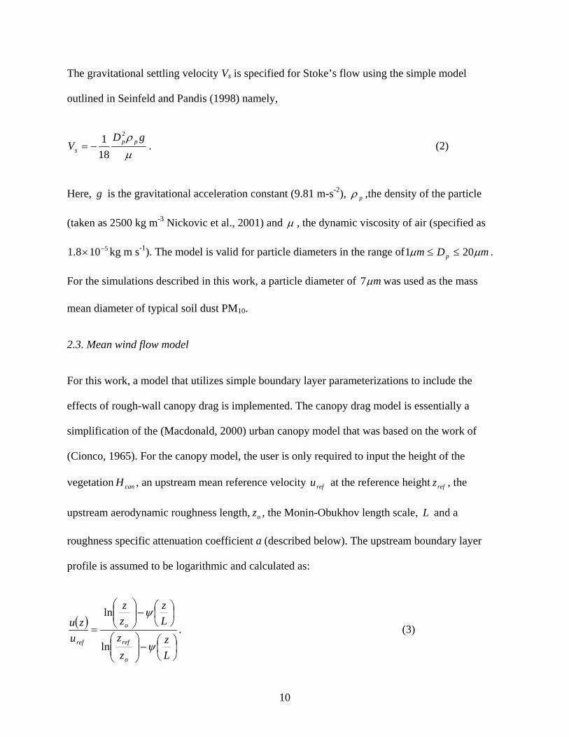
The gravitational settling velocity Vs is specified for Stoke’s flow using the simple model
outlined in Seinfeld and Pandis (1998) namely,
μρ gD
V pps
2
181
−= . (2)
Here, g is the gravitational acceleration constant (9.81 m-s-2), pρ ,the density of the particle
(taken as 2500 kg m-3 Nickovic et al., 2001) and μ , the dynamic viscosity of air (specified as
kg m s5−108.1 × -1). The model is valid for particle diameters in the range of mDm p μμ 201 ≤≤ .
For the simulations described in this work, a particle diameter of mμ7
H
z
was used as the mass
mean diameter of typical soil dust PM10.
2.3. Mean wind flow model
For this work, a model that utilizes simple boundary layer parameterizations to include the
effects of rough-wall canopy drag is implemented. The canopy drag model is essentially a
simplification of the (Macdonald, 2000) urban canopy model that was based on the work of
(Cionco, 1965). For the canopy model, the user is only required to input the height of the
vegetation , an upstream mean reference velocity at the reference height , the
upstream aerodynamic roughness length, , the Monin-Obukhov length scale,
can refu refz
o L and a
roughness specific attenuation coefficient a (described below). The upstream boundary layer
profile is assumed to be logarithmic and calculated as:
( )
⎟⎠⎞
⎜⎝⎛−⎟⎟
⎠
⎞⎜⎜⎝
⎛
⎟⎠⎞
⎜⎝⎛−⎟⎟
⎠
⎞⎜⎜⎝
⎛
=
Lz
zz
Lz
zz
uzu
o
ref
o
ref ψ
ψ
ln
ln. (3)
10
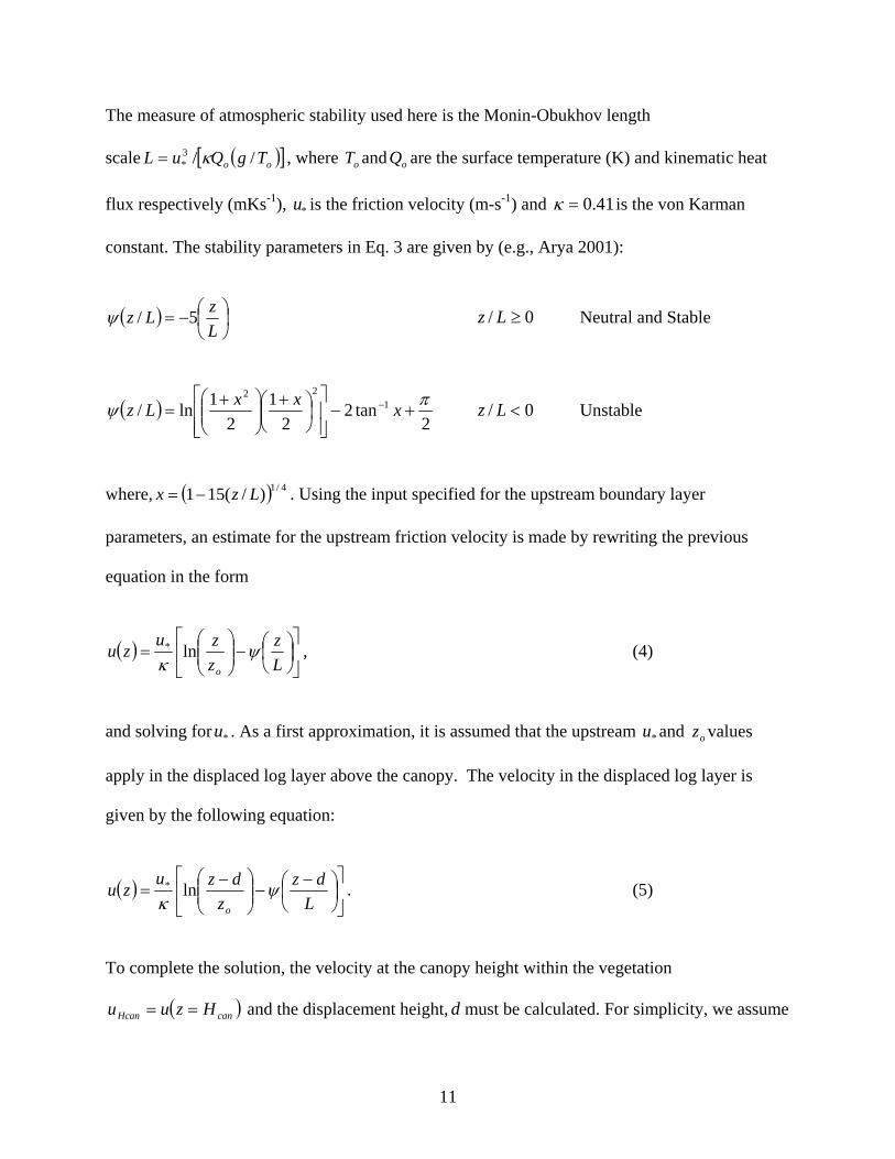
The measure of atmospheric stability used here is the Monin-Obukhov length
scale , where and are the surface temperature (K) and kinematic heat
flux respectively (mKs
( )[ ]3
u 41.0
oo TgQuL //* κ= oT oQ
-1), is the friction velocity (m-s*-1) and =κ is the von Karman
constant. The stability parameters in Eq. 3 are given by (e.g., Arya 2001):
( ) ⎟⎠⎞
⎜⎝⎛−=
LzLz 5/ψ Neutral and Stable 0/ ≥Lz
( )2
tan22
12
1ln/ 122 πψ +−⎥⎥⎦
⎤
⎢⎢⎣
⎡⎟⎠⎞
⎜⎝⎛ +⎟⎟⎠
⎞⎜⎜⎝
⎛ += − xxxLz 0/ <Lz Unstable
where, . Using the input specified for the upstream boundary layer
parameters, an estimate for the upstream friction velocity is made by rewriting the previous
equation in the form
( 4/1)/(151 Lzx −= )
( ) ⎥⎦
⎤⎢⎣
⎡⎟⎠⎞
⎜⎝⎛−⎟⎟
⎠
⎞⎜⎜⎝
⎛=
Lz
zzuzuo
ψκ
ln* , (4)
and solving for . As a first approximation, it is assumed that the upstream and values
apply in the displaced log layer above the canopy. The velocity in the displaced log layer is
given by the following equation:
*u *u oz
( ) ⎥⎦
⎤⎢⎣
⎡⎟⎠⎞
⎜⎝⎛ −
−⎟⎟⎠
⎞⎜⎜⎝
⎛ −=
Ldz
zdzu
zuo
ψκ
ln* . (5)
To complete the solution, the velocity at the canopy height within the vegetation
and the displacement height, must be calculated. For simplicity, we assume ( )== dcanHcan Hzuu
11
that the flow within the canopy is independent of atmospheric stability and follow (Cionco,
1965), assuming that an exponential solution applies within the canopy and that the displaced log
profile applies above the canopy. The exponential solution is given by
( ) ⎥⎦
⎤⎢⎣
⎡⎟⎟⎠
⎞⎜⎜⎝
⎛−= 1exp
canHcan H
zauzu . (6)
Here, a is the attenuation coefficient associated with specific types of roughness (Cionco, 1978).
Larger values of a indicate an increased momentum sink associated with the roughness. The
attenuation coefficient is dependant on a wide range of factors including: the flexibility, the
shape, surface area and spacing of the roughness elements(Cionco, 1965). Typical values of a for
different types of vegetation are provided in Table 1. Some generalizations for the calculation of
the attenuation coefficient exist such as (Macdonald, 2000) for idealized building arrays and
(Cionco, 1965) for vegetation. Generally, however, a values must be obtained by measuring
velocity profiles within the canopy and fitting an exponential solution to them.
Up to this point, the method is very similar to the technique proposed by (Macdonald, 2000).
Here we diverge from Macdonald’s method by forcing the velocities and the slopes of the
velocity profiles to be matched at the canopy height . This simplifies Macdonald’s method
by eliminated a matching layer and fixes the values of andu . The displacement
height d and are then obtained by solving the following two equations:
canH
d
u
Hcan
Hcan
*uua
LdH
dHH Hcan
can
can κφ =⎟
⎠⎞
⎜⎝⎛ −
− (7)
⎟⎠⎞
⎜⎝⎛ −
−⎟⎟⎠
⎞⎜⎜⎝
⎛ −=
LdH
zdHuu can
o
canHcan ψ
κln* . (8)
12
Where the universal stability functions are given by (Arya 2001) as:
⎟⎠⎞
⎜⎝⎛ −
+=⎟⎠⎞
⎜⎝⎛ −
Ldz
Ldz 51φ Neutral and Stable 0/ ≥Lz
4/1
151−
⎟⎠⎞
⎜⎝⎛ −−=⎟
⎠⎞
⎜⎝⎛ −
Ldz
Ldzφ 0/ <Lz Unstable
Since Eq. 7 and are not explicit in , a numerical method is required in to obtain a solution. For
the solutions given here, a simple iterative bisection method was used (Chapra and Canale,
2006). Figure 2 shows an example of three different velocity profiles with identical input
parameters except for upstream stability.
d
2.4. Turbulence model
The vertical turbulent flux of particle concentration within the vegetation is modeled using a
simple gradient method, namely
zcKcw zz ∂∂
=− ''
as shown in Eq. 1. In the present model, it is assumed that the concentration diffusion coefficient
is the same as the momentum diffusion coefficient. Hence, upstream of the canopy a simple
log law boundary layer model is used where is specified based on Monin-Obukhov similarity
as
zzK
K
)
zz
( LzzuK zz /
*
φκ
= . (9)
13
Within the canopy, a mixing length model that is independent of atmospheric stability is
assumed and specified in the form:
zuK
zulwu zz ∂
∂=⎟
⎠⎞
⎜⎝⎛∂∂
=−2
2'' . (10)
In Eq. 10, the velocity gradient is calculated directly using finite differences from the mean flow
field. Above the canopy, the mixing length scale is modeled as the sum of the canopy length
scale (lcu) and the surface layer length scale (lsl) (i.e. l slcu ll += ), where the mixing length is
given by
sll
( )
⎟⎠⎞
⎜⎝⎛ −
−=
Ldzdzklsl
φ. (11)
Within the canopy, the mixing length is broken up into an upper ( 3 ) and lower
( 3 ) canopy mixing length following Cionco (1965). For the
mixing length is assumed constant and modeled following (Macdonald, 2000) by substituting
Eq. 6 into Eq. 10 and solving for the mixing length at
cul .0/ >canHz
cll .0/ ≤canHz cancan HzH ≤<3.0 ,
canHz = . This model assumes that the
shear stress at the canopy height is the same as the shear stress in the surface layer. This yields
the following approximation for the mixing length in the upper part of the canopy:
Hcan
cancu au
uHl *= . (12)
For , the mixing length is assumed to increase linearly from zero at the ground to
the value predicted by Eq. 12 at
3.0/ ≤canHz
3.0/ =canHz . It should be noted that although the conditions in
14
the canopy are assumed independent of stability, a dependence of stability is introduced by using
the value of d obtained by matching the exponential and logarithmic curves as described in
Section 2.3 above.
2.5 Numerical Implementation
The velocity parameterizations described above assume horizontal homogeneity. In the actual
simulations, there was a finite fetch F between the road and the start of the roughness elements
(see Fig. 1b). A rough wall turbulent boundary layer (Eq. 3, with zo/Hcan = 0.02) was assumed
upwind of the vegetative canopy; the flow was immediately assumed to follow the canopy
profiles parameterizations within the vegetation. To deal with this discontinuity, the initial flow
field was forced to be mass consistent via a classical variational analysis procedure (Sherman,
1978). The resulting mass consistent wind field and turbulence models described above were
input into a numerical simulation of Eq. 1 using Matlab subject to the following boundary
conditions: at the inlet and outlet; 0/ =dxdc 0/ =dzdc at the top of the domain and at the
ground. The dust cloud was initialized with a uniform concentration of c
0=c
o = 75 mg-m-3 over a
rectangular region centered on the road with a height Hdc and width Wdc. The height was varied
throughout the simulations but the cloud width was fixed at 3 m corresponding to the width of a
typical travel lane. The spatial domain was rectangular with a streamwise length of 630m and a
height of 50m. The fetch F from the center of the road to the upwind edge of the domain was
30m for the simulations.
The spatial domain was discretized using finite volumes (Versteeg and Malalasekera, 1995). The
advective terms were modeled by a first order upwind finite difference. The diffusive terms were
15
modeled using second order central differences. The body terms are exact and the temporal
dependence of Eq. 1 is modeled using an Alternating Direction Implicit (ADI) technique
(Anderson, 1995). Variable time steps are used during a typical 125s simulation. Smaller time
steps of the order of 0.01s are used in the first 10s. Larger time steps of the order of 0.25 to 1s
are used for the rest of the simulation. To minimize computational effort, a non-uniform mesh is
utilized by solving Eq. 1 on a logarithmic mesh (Anderson, 1995). The grid is stretched both in
the vertical and horizontal directions with stretching factors of 0.07 and 0.004 respectively. The
minimum grid sizes in vertical and horizontal directions were 5.6 cm and 50.8 cm. A typical
simulation runs on a Celeron PC laptop in about two and half minutes. This involves about
30,000 nodes (300 in the streamwise direction and 100 in the vertical) and 500 time steps. The
large number of time steps is necessary to ensure mass conservation of the dust particles. This is
done by running each time step twice, once without vegetative deposition and another with
vegetative deposition (Boybeyi, 2000; Schieffe and Morris, 1993).
3. Results
3.1. Turbulence Model
Figure 3 illustrates the performance of the mixing length model (Eq. 12) against a number of
experimental data sets. The data set was compiled from a wide range of wind tunnel and field
experiments described in the figure caption. An average value for the in-canopy mixing length
was calculated directly from the available data sets using Eq. 10 and then compared to Eq. 12.
With the exception of the (Seginer et al., 1976) wind tunnel study of flow through surface
mounted cylinders, the data appear to be quite linear over the range ( ) 36.0/076.0 * << auu Hcan .
16
( ) 07.0/7.0/ +*Linear regressions of the data yields a best fit of = Hcancancu auuH
* ==
* ==
*
l with R2 =
0.89. Hence, the model tends to under predict the mixing length in the canopy.
Figure 4 shows the modeled momentum fluxes in the canopy compared to measured fluxes
separated into (a) low, (b) medium and (c) high attenuation coefficients. The model matches the
data quite well in the upper 25% of the canopy, however in the lower 75%, the model can under
predicts fluxes by as much as ~50%.
3.2. Road Dust Simulation
A number of factors determine the fraction of the initial dust cloud deposited onto roughness
elements. In this work, we focus on the effects of roughness length, atmospheric stability and
deposition effectiveness of the canopy. In order to maintain this focus, a test canopy with
dimensions similar to a real unpaved road was implemented as described in section 2.5. In
addition, the dimensionless initial dust cloud height was and a
dimensionless fetch was utilized. This example case is representative of
relatively small bushes adjacent to an unpaved road (typical of an arid environment), but would
not be representative of a dirt road near the edge of a tall forest where
2/ candc HHH
2/ canHFF
H and . Figure
5a shows the effect of three different attenuation coefficients on the mass fraction of suspended
particles (M
1<<F *
A
s/Mo) as a function of dimensionless advection time for neutral atmospheric stability.
Here Mo is the initial mass in the dust cloud and Ms in the mass remaining in the air at some later
time. In this simulation, the deposition term V was held constant such that the effect of the
modeled wind profile and turbulence within the canopy were isolated. As expected, more dense
canopies result in higher attenuation coefficients, reduced wind speed within the canopy and
enhanced deposition. Similarly, Fig. 5b shows the effect of atmospheric stability on a canopy
Vd
17
with a moderate attenuation coefficient (a = 2.25). For the case shown (with 2 ms-1 wind speed
upstream and 2 m tall canopy) 30 m downstream of the road, there is a 67% reduction in Ms/Mo
for the stable atmospheric stability case compared to the unstable case.
4. Discussion
Understanding the effectiveness of particle deposition onto various types of roughness is of great
importance. A bulk measure of this effectiveness that utilizes the methodology outlined in this
paper can be obtained by considering the ratio of the turbulent diffusion time scale to a
deposition time scale. Here, the deposition time scale refers to the horizontal deposition
associated primarily with impaction of the dust cloud onto roughness elements (i.e. “filtering”)
and may be defined as . The inverse of this deposition time scale is also referred to
by (Veranth et al., 2007) as the clearance frequency because it represents the fraction of particles
in a control volume that are removed per unit time by deposition to vegetation and other
surfaces. Another time scale is associated with the time required for a particle to move out of the
canopy (over a height H
( ) 1−= vdd AVτ
can) through turbulent diffusion can be defined as ( )canzzcant HKH /2=τ .
The ratio of these two time scales is
d
t
canzz
canVd
HKHAV
ττ
==Τ)(
2* . (13)
In Eq. 13, is the turbulent diffusivity at the top of the canopy. ( canzz HK ) *Τ provides a bulk
metric to determine the expected deposition rate effectiveness of a canopy associated with the
horizontal advection of dust. is dependent on the specific geometry of the canopy, particle
deposition physics, as well as atmospheric turbulence. Considering the limits of is particularly
useful. As
*Τ
*Τ
∞→dt ττ / , we expect that the suspended mass fraction Ms / Mo → 0because most of
the particles should be removed from the air stream before they diffuse out of the canopy.
18
Similarly, as 0/ →dt ττ , Ms/Mo should approach the well mixed case where horizontal
deposition is of little importance (e.g. far downwind in Fig. 1a) since the particulate cloud
disperses rapidly compared to the time required to deposit particulate matter onto roughness
elements. Figure 6 shows Ms/Mo as a function of the deposition rate effectiveness on a semi-log
plot. The plot is composed of three distinct regimes: (1) 1* <Τ , turbulence rapidly mixes
particles and the Ms/Mo decreases slowly with increasing *Τ , (2) , the M101 * <Τ< s/Mo
decreases rapidly as the importance of deposition increases and (3) , M10* >Τ s/Mo begins to
decrease more slowly in response to very low particle concentrations in the canopy.
Figure 7 shows the effect of the ratio of the initial dust cloud height to the vegetative canopy
height, *H on mass fraction suspended at equivalent non-dimensional times after the start of the
simulations. As expected, for short dust clouds 1* <H , much of the dust is removed as it is
advected horizontally through the roughness elements. The mass fraction suspended rapidly
increases with increasing *H until 4~*H as the importance of the horizontal impaction on the
roughness elements decreases. For 4* >H , horizontal removal is insignificant and the problem
approaches the classical well mixed vertical deposition onto a surface case.
Figure 8 summarizes the model’s utility to help describe the effect of roughness and atmospheric
stability on deposition in vegetative or building canopies. For highly unstable atmospheric
conditions, significant changes in roughness result in very small changes in deposition. While for
stable atmospheric conditions, relatively small increases in roughness result in significantly
enhanced deposition. For example, consider the hypothetical canopy with an attenuation
coefficient of 2.5 shown in Fig. 8. The decrease in Ms/Mo from z/L = -2 to z/L = -0.5 is less than
19
~8%, while the decrease from z/L = 0.5 to z/L = 2 is ~35%. In addition, Figure 8 helps explain
the discrepancy between the convective low vegetation Ft. Bliss results and the high roughness
stable conditions for the Dugway Proving Ground experiment described in the introduction. The
Ft. Bliss case would reside in the lower left corner of Fig. 8 where deposition is least, while the
Dugway case would be in the upper more central part of the figure where deposition is
substantially increased.
One of the advantages of using the Eulerian transport model given in Eq. 1, is that it allows one
to analyze and understand the contribution of each of the terms to the total transport. Figure 9
shows the contributions of the various terms from Eq. 1 twenty meters downwind of the leading
edge of the canopy with most of the plume still contained within the vegetation. Figure 9a shows
the contribution of the plume 20 seconds after the start of the simulation. As expected, the
deposition term (term V) is always a sink within the canopy (ie. negative values) and zero above.
The other three terms on the right hand side of Eq. 1(term II, III and IV) may be positive or
negative depending on vertical location and time. As shown in Fig. 9a, the mean streamwise
advection is the dominant transport term. The sign of the advection term is positive near the
ground (0<z/Hcan<0.14) and negative for z/Hcan > 0.14. Since the velocities are nearly constant in
the streamwise direction, the advection term is dominated by the streamwise gradient of the
concentration. Hence, where term II is positive, the concentration is increasing with streamwise
distance and where term II is negative, the concentration must be decreasing. Due to the
directional behavior of advection, this is equivalent to stating that at higher elevations the dust
plume is advected downwind at a greater rate than at the bottom of the the canopy where
velocities are very low. That is, the higher locations are observing the departure of the bulk of
the dust plume, while lower heights are still observing the cloud’s arrival.
20
The vertical turbulent diffusion (term III) is dependent on the gradient of the product of the local
vertical concentration gradient and Kzz. Since Kzz increases monotonically, term III follows the
curvature of the concentration profile. Hence, term III is positive below the lowest inflection
point in the concentration profile (z/Hcan<0.1), negative from 0.1<z/Hcan<0.22 and positive again
z/Hcan>0.22. This is intuitively expected, as the concentration will decreases near the peak and
increase at the tails due to diffusion. Since the settling velocity Vs is constant for a given
simulation (one particle size and type), the gravity settling (term IV) is only a function of the
concentration gradient. Hence, for small particles, term IV takes on small positive values below
the peak and negative values above the peak.
4. Conclusions
In this paper, we describe the development of a quasi-2D Eulerian atmospheric diffusion model
applied to the transport and deposition of fugitive dust near an unpaved road. Specifically, this
work addresses a gap in the literature associated with transport and deposition in the “impact
zone” where horizontal deposition may be of importance. The primary attribute of the present
modeling technique is that a user can investigate the effects of various deposition scenarios
associated with different roughness and atmospheric stabilities, while only needing to supply a
small the number of difficult to obtain input parameters. Since the model also runs rapidly, a
large number of cases can be run parametrically to investigate the importance various input
variables; allowing decision makers more information regarding planning scenarios.
The model also provides insight toward reconciling the differences between field experiments in
the literature where large differences were observed in deposition rates for different stabilities
21

and canopy roughnesses. The primary limitation of the model is the ability to accurately
determine the vegetative deposition parameter or so-called clearance frequency. To understand
the clearance frequency better, a dimensionless parameter called the transport effectiveness is
identified and the limiting cases discussed. In general, the model captures the essential physics of
near source dust transport and provides a tool that that can efficiently simulate site-specific
conditions in practical situations.
Acknowledgements
This work was sponsored by the Strategic Environmental Research and Development Program
project CP1190 and by Southwest Center for Environmental Research and Policy project A-02-7
and A-04-03. We also wish to thank Mr. Thomas Booth for his hard work and contributions to
the mean wind model.
22
References:
Anderson, J.D., 1995. Computational fluid dynamics. McGraw Hill, New York, 547 pp. Aylor, D.E. and Flesch, T.K., 2001. Estimating spore release rates using a Lagrangian stochastic
simulation model. J. Appl. Meteor., 40(7): 1196-1208. Belcher, S.E., 2005. Mixing and transport in urban areas. Phil. Trans. R. Soc. A, 363: 2947-
2968. Boybeyi, Z., 2000. Mesoscale atmospheric dispersion. WIT Press, Boston, 448 pp. Britter, R.E. and Hanna, S.R., 2003. Flow and dispersion in urban areas. Annu. Rev. Fluid
Mech., 35: 469-496. Brunet, Y., Finnigan, J.J. and Raupach, M.R., 1994. A wind tunnel study of air flow in waving
wheat: single-point velocity statistics. Bound.-Layer Meteor., 70: 95-132. Chamberlain, A.C., 1975. The movement of particles in plant communities. Vegetation and the
Atmosphere, 1: 155-203. Chapra, S.C. and Canale, R.P., 2006. Numerical Methods for Engineers. McGraw Hill, New
York. Cionco, R.M., 1965. Mathematical model for air flow in vegetative canopy. J. Appl. Meteorol.,
4: 517-522. Cionco, R.M., 1978. Analysis of canopy index values for various canopy densities. Boundary-
Layer Meteorology, 15(1): 81-93. Davidson, C.I., Phalen, R.F. and Solomon, P.A., 2005. Airborne Particulate Matter and Human
Health: A Review. Aerosol Science & Technology, 39(8): 737-749. Denmead, O.T. and Bradley, E.F., 1987. On scalar transport in plant canopies. Irrig. Sci., 8: 131-
149. Etyemezian, V. et al., 2004. Deposition and removal of fugitive dust in the arid southwestern
United States: measurements and model results. J. Air Waste Manag. Assoc., 54(9): 1099-1111.
Finnigan, J.J., 2000. Turbulence in plant canopies. Annu. Rev. Fluid Mech., 32: 519-571. Harley, R.A., Hunts, S.E. and Cass, G.R., 1989. Strategies for the control of particulate air
quality: least-cost solutions based on receptor-oriented models. Environmental Science & Technology, 23(8): 1007-1014.
Harman, I.N. and Finnigan, J.J., 2007. A simple unified theory for flow in the canopy and roughness sublayer. Boundary-Layer Meteorology, 123(2): 339-363.
Kaimal, J.C. and Finnigan, J.J., 1994. Atmospheric Boundary Layer Flows: Their Structure and Measurement. Oxford University Press US.
Kastner-Klein, P. and Rotach, M.W., 2004. Mean flow and turbulence characteristics in an urban roughness sublayer. Bound.-Layer Meteor., 111: 55-84.
Macdonald, R.W., 2000. Modelling the mean velocity profile in the urban canopy layer. Bound.-Layer Meteor., 97: 25-45.
Nicholson, K.W., 1988. The dry deposition of small particles: A review of experimental measurements. Atmospheric Environment, 22(12): 2653-2666.
Nickovic, S., Kallos, G., Papadopoulos, A. and Kakaliagou, O., 2001. A model for prediction of desert dust cycle in the atmosphere. Journal of Geophysical Research, 106(D16): 18113-18130.
23
Novak, M.D., Warland, J.S., Orchansky, A.L., Ketler, R. and Green, S., 2000. Wind Tunnel And Field Measurements Of Turbulent Flow In Forests. Part I: Uniformly Thinned Stands. Bound.-Layer Meteor., 95(3): 457-495.
Pace, T.G., 2005. Methodology to estimate the transportable fraction (TF) of fugitive dust emissions for regional and urban scale air quality analyses, USEPA.
Poggi, D., Porporato, A., Ridolfi, L., Albertson, J.D. and Katul, G.G., 2004. The effect of vegetation density on canopy sub-layer turbulence. Bound.-Layer Meteor., 111: 565-587.
Ramaswami, A., Milford, J.B. and Small, M.J., 2005. Integrated environmental modeling: pollutant transport, fate and risk in the environment. Wiley, 678 pp.
Raupach, M.R., P.A., C. and Legg, B.J., 1986. Experiments on scalar dispersion within a model plant canopy. Part I: The turbulence structure. Bound.-Layer Meteor., 35(21-52).
Raupach, M.R. and Thom, A.S., 1981. Turbulence in and above plant canopies. Annu. Rev. Fluid Mech., 13: 97-129.
Raupach, M.R., Woods, N., Dorr, G., Leys, J.F. and Cleugh, H.A., 2001. The entrapment of particles by windbreaks. Atmos. Environ., 35: 3373-3383.
Schieffe, R.D. and Morris, R.E., 1993. A review of the development and application of the urban airshed model. Atmos. Environ., 27B: 23-29.
Seginer, I., Mulhearn, P.J., Bradley, E.F. and Finnigan, J.J., 1976. Turbulent flow in a model plant canopy. Bound.-Layer Meteor., 10: 423-453.
Sehmel, G.A., 1980. Particle and gas dry deposition- A review. Atmospheric Environment, 14(9): 983-1011.
Seinfeld, J.H. and Pandis, S.N., 1998. Atmospheric chemistry and physics - from air pollution to climate change. Wiley, Hoboken, 1203 pp.
Shaw, R.H., Silversides, R.H. and Thurtell, G.W., 1974. Some observations of turbulence and turbulent transport within and above plant canopies. Bound.-Layer Meteor., 5: 429-449.
Sherman, C.A., 1978. A mass-consistent model for wind fields over complex terrain. J. Appl. Meteor., 17(3): 312-319.
Slinn, W.G.N., 1982. Predictions for particle depostion to vegetative canopies. Atmos. Environ., 16: 1785-1794.
Veranth, J.M., Pardyjak, E.R. and Seshadri, G., 2003. Vehicle-generated Dust Transport: Analytic Models and Field Study. Atmos. Environ., 37: 2295-2302.
Veranth, J.M., Speckart, S.O., Yin, F., Etyemezian, V. and Pardyjak, E.R., 2007. Near-source deposition of vehicle-generated fugitive dust on vegetative surfaces and buildings, part II: Field deposition measurements and model validation submitted to Atmos. Environ.
Versteeg, H.K. and Malalasekera, W., 1995. An introduction to computational fluid dynamics–the finite volume approach. Longman Scientific & Technical, 257 pp.
Watson, J.G. and Chow, J.C., 1994. Clear sky visibility as a challenge for society. Annu. Rev. Energy Environ., 19: 241-266.
Watson, J.G. and Chow, J.C., 2000. Reconciling Urban Fugitive Dust Emissions Inventory and Ambient Source Contribution Estimates: Summary of Current Knowledge and Needed Research. DRI Document.
Wilson, J.D., Ward, D.P., Thurtell, G.W. and Kidd, G.E., 1982. Statistics of atmospheric turbulence within and above a corn canopy. Bound.-Layer Meteor., 24: 495-519.
24
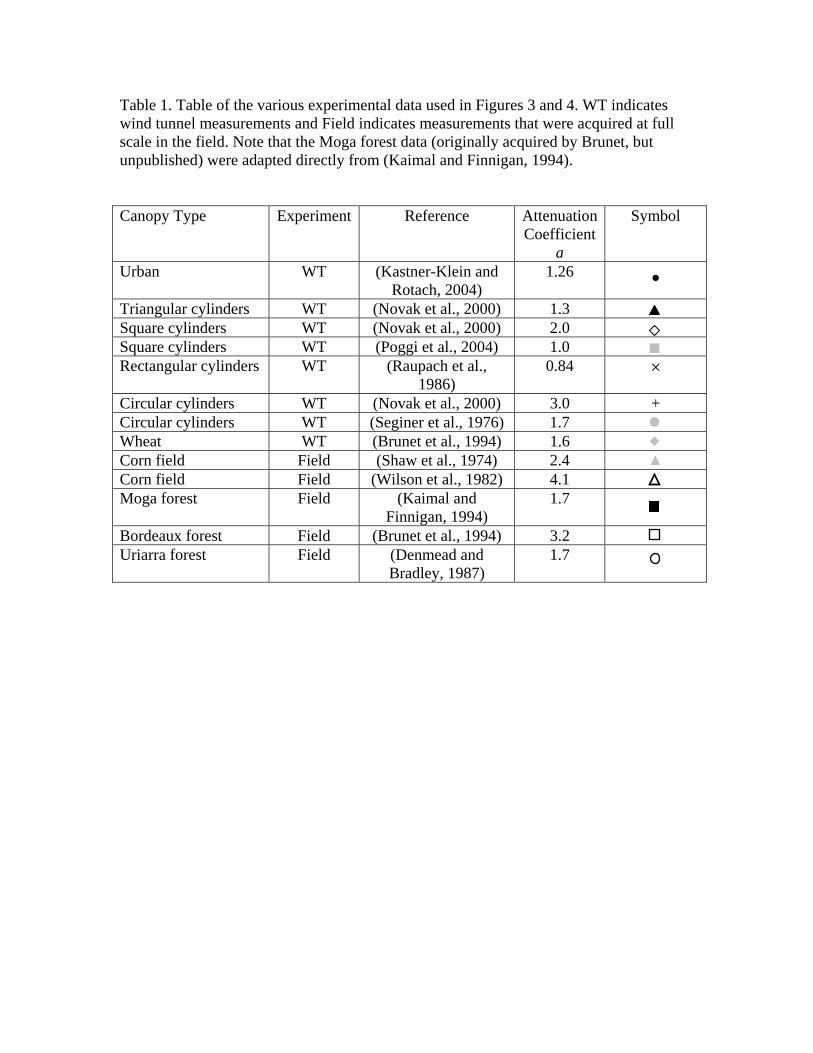
Table 1. Table of the various experimental data used in Figures 3 and 4. WT indicates wind tunnel measurements and Field indicates measurements that were acquired at full scale in the field. Note that the Moga forest data (originally acquired by Brunet, but unpublished) were adapted directly from (Kaimal and Finnigan, 1994).
Canopy Type Experiment Reference Attenuation Coefficient
a
Symbol
Urban WT (Kastner-Klein and Rotach, 2004)
1.26 • Triangular cylinders WT (Novak et al., 2000) 1.3 Square cylinders WT (Novak et al., 2000) 2.0 Square cylinders WT (Poggi et al., 2004) 1.0 Rectangular cylinders WT (Raupach et al.,
1986) 0.84 ×
Circular cylinders WT (Novak et al., 2000) 3.0 + Circular cylinders WT (Seginer et al., 1976) 1.7 Wheat WT (Brunet et al., 1994) 1.6 Corn field Field (Shaw et al., 1974) 2.4 Corn field Field (Wilson et al., 1982) 4.1 Moga forest Field (Kaimal and
Finnigan, 1994) 1.7
Bordeaux forest Field (Brunet et al., 1994) 3.2 Uriarra forest Field (Denmead and
Bradley, 1987) 1.7
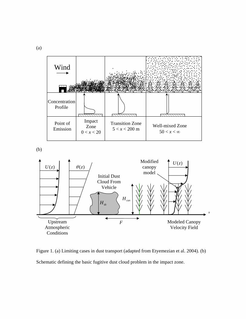
(a)
Impact Zone
0 < x < 20
Point of Emission
Concentration Profile
Wind
Transition Zone 5 < x < 200 m
Well-mixed Zone 50 < x < ∞
(b)
Upstream Atmospheric Conditions
)(zU )(zθ)(zU
dcH canH
Modifiedcanopy model
Initial Dust Cloud From
Vehicle
Modeled Canopy Velocity Field
x
F
Figure 1. (a) Limiting cases in dust transport (adapted from Etyemezian et al. 2004). (b)
Schematic defining the basic fugitive dust cloud problem in the impact zone.
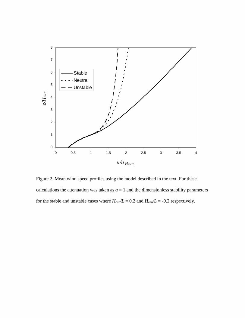
0
1
2
3
4
5
6
7
8
0 0.5 1 1.5 2 2.5 3 3.5 4
u/u Hcan
z/Hca
n
StableNeutralUnstable
Figure 2. Mean wind speed profiles using the model described in the text. For these
calculations the attenuation was taken as a = 1 and the dimensionless stability parameters
for the stable and unstable cases where Hcan/L = 0.2 and Hcan/L = -0.2 respectively.
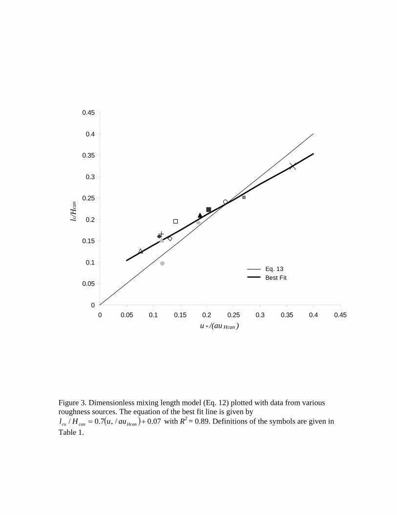
0
0.05
0.1
0.15
0.2
0.25
0.3
0.35
0.4
0.45
0 0.05 0.1 0.15 0.2 0.25 0.3 0.35 0.4 0.45u * /(au Hcan )
lc /H
can
Eq. 13Best Fit
Figure 3. Dimensionless mixing length model (Eq. 12) plotted with data from various roughness sources. The equation of the best fit line is given by
with R( ) 07.0/7.0/ * += Hcancancu auuHl 2 = 0.89. Definitions of the symbols are given in Table 1.
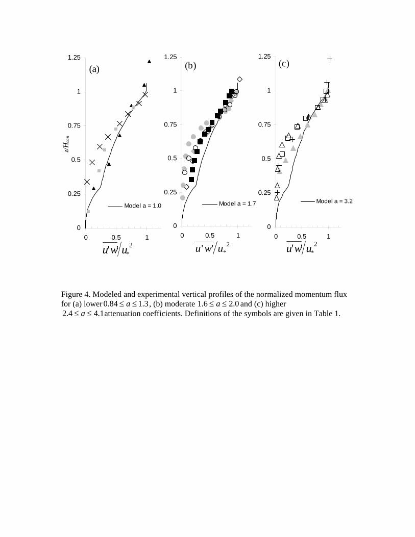
0
0.25
0.5
0.75
1
1.25
0 0.5 1
z/Hca
n
2*'' uwu
(a)
Model a = 1.0
0
0.25
0.5
0.75
1
1.25
0 0.5 12
*'' uwu
(b)
Model a = 1.7
0
0.25
0.5
0.75
1
1.25
0 0.5 12
*'' uwu
(c)
Model a = 3.2
Figure 4. Modeled and experimental vertical profiles of the normalized momentum flux for (a) lower , (b) moderate 3.184.0 ≤≤ a 0.26.1 ≤≤ a and (c) higher
attenuation coefficients. Definitions of the symbols are given in Table 1. 1.44.2 ≤≤ a

0
0.2
0.4
0.6
0.8
1
1.2
0 10 20 30 40 500
0.2
0.4
0.6
0.8
1
1.2
0 10 20 30 40 5
tU Hcan / H can
Ms/M
o
a=1.00
0
Stable
Neutral
Unstable
a=2.25
a=3.75
tU Hcan / H can
Ms/M
o
(a) (b)
Figure 5. Mass fraction of suspended particles as a function of non-dimension advection
time for (a) three canopies with different attenuation coefficients (and corresponding T* =
8.5, 17, 27 for a = 1.0, 2.25 and 3.75) and neutral stability; (b) and for a canopy with a =
2.25 and T* = 17 with different atmospheric stabilities (stable: Hcan/L = 0.2, unstable:
Hcan/L = -0.2).
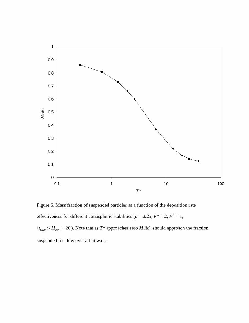
0
0.1
0.2
0.3
0.4
0.5
0.6
0.7
0.8
0.9
1
0.1 1 10 100
T*
Ms/M
o
Figure 6. Mass fraction of suspended particles as a function of the deposition rate
effectiveness for different atmospheric stabilities (a = 2.25, F* = 2, H* = 1,
). Note that as T* approaches zero M20/ =canHcan Htu s/Mo should approach the fraction
suspended for flow over a flat wall.
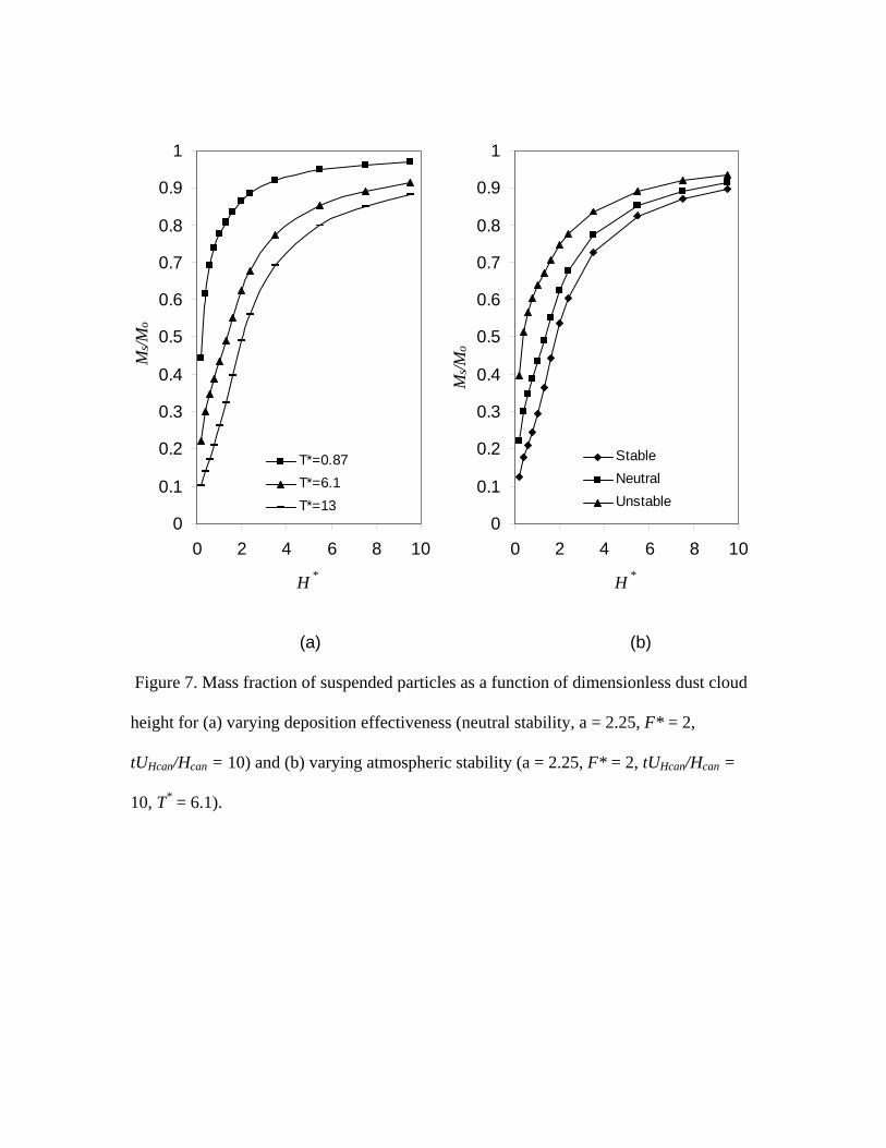
0
0.1
0.2
0.3
0.4
0.5
0.6
0.7
0.8
0.9
1
0 2 4 6 8 10
H *
Ms/M
o
T*=0.87T*=6.1T*=13
0
0.1
0.2
0.3
0.4
0.5
0.6
0.7
0.8
0.9
1
0 2 4 6 8 10
H *
Ms/M
oStableNeutralUnstable
(a) (b)
Figure 7. Mass fraction of suspended particles as a function of dimensionless dust cloud
height for (a) varying deposition effectiveness (neutral stability, a = 2.25, F* = 2,
tUHcan/Hcan = 10) and (b) varying atmospheric stability (a = 2.25, F* = 2, tUHcan/Hcan =
10, T* = 6.1).
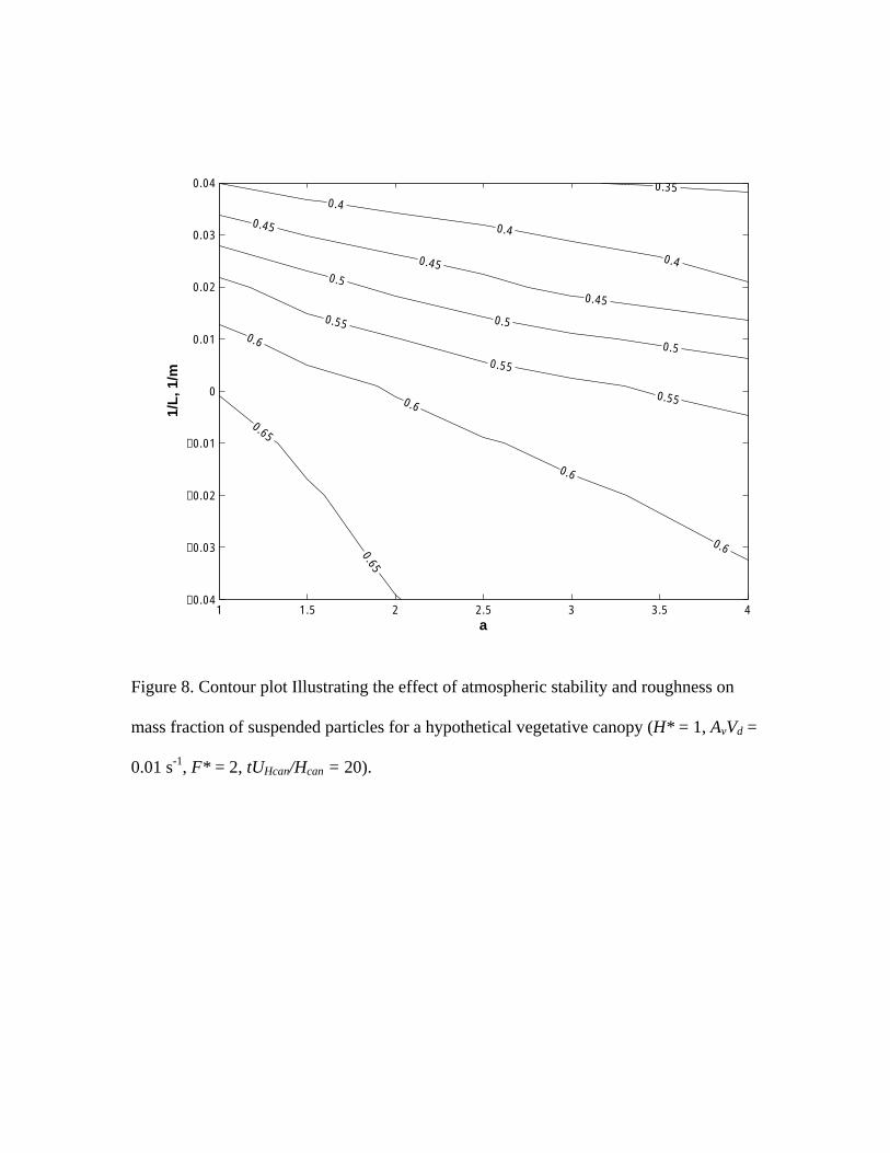
0.350.4
0.4
0.4
0.45
0.45
0.45
0.5
0.5
0.5
0.55
0.55
0.55
0.6
0.6
0.6
0.60.65
0.65
a
1/L
, 1/m
1 1.5 2 2.5 3 3.5 4−0.04
−0.03
−0.02
−0.01
0
0.01
0.02
0.03
0.04
Figure 8. Contour plot Illustrating the effect of atmospheric stability and roughness on
mass fraction of suspended particles for a hypothetical vegetative canopy (H* = 1, AvVd =
0.01 s-1, F* = 2, tUHcan/Hcan = 20).
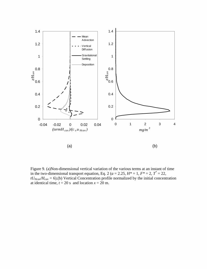
0
0.2
0.4
0.6
0.8
1
1.2
1.4
-0.04 -0.02 0 0.02 0.04(termH can )/(c o u Hcan )
z/Hca
nMeanAdvection
VerticalDiffusion
GravitationalSettling
Deposition
0
0.2
0.4
0.6
0.8
1
1.2
1.4
0 1 2 3 4
mg/m 3
z/Hca
n
(a) (b)
Figure 9. (a)Non-dimensional vertical variation of the various terms at an instant of time in the two-dimensional transport equation, Eq. 2 (a = 2.25, H* = 1, F* = 2, T* = 22, tUHcan/Hcan = 6).(b) Vertical Concentration profile normalized by the initial concentration at identical time, t = 20 s and location x = 20 m.

APPENDIX 2
1
Near-source Deposition of Vehicle-Generated Fugitive Dust on Vegetation and Buildings Part
2: Field Measurements and Model Validation
Authors and Affiliations John M. Veranth1, Scott O. Speckart2, Fang Yin3, Vic Etyemezian4, Eric R. Pardyjak2
1. Department of Pharmacology and Toxicology, University of Utah, Salt Lake City, Utah 2. Department of Mechanical Engineering, University of Utah, Salt Lake City, Utah 3. Department of Chemical Engineering, University of Utah, Salt Lake City, Utah 4. Atmospheric Sciences Division, Desert Research Institute, Las Vegas, Nevada
Manuscript for Submission to Atmospheric Environment
October 16, 2007
Corresponding Author Contact Information John M. Veranth Department of Pharmacology and Toxicology, University of Utah 30 South 2000 East, Room 112 Skaggs Hall Salt Lake City, UT 84112-5820 Phone: 801-581-3789 Fax: 801-585-5111 Email: [email protected]
2
Abstract
The near-source removal of vehicle-generated fugitive dust was studied by deposition measurements on test surfaces and by computational simulations to improve the scientific basis for effective air quality management strategies. Deposition was measured under summer and winter meteorological conditions using on both artificial vegetation and flat substrates. Deposition velocity calculated from aerosol concentration and scanning electron microscopy imaging of polycarbonate substrates that had been exposed while facing in orthogonal directions was approximately isotropic suggesting that impaction and interception due to advection and small-scale turbulence are important. A computational model for fugitive dust deposition, described in the companion Part 1 paper, was used to reanalyze data from two published field studies that compared dust flux adjacent to an unpaved road versus approximately 100 m downwind. The model considers deposition velocity, effective deposition surface area, the height of the canopy, and wind profile. Model simulation results were compared to field measurements and the effects of alternative site conditions are summarized. Canopy height relative to the initial dust cloud height, the area of surface roughness available for deposition, and the atmospheric stability are predicted to affect the partitioning of the initially suspended dust between transport and near-source redeposition. This work supports the hypothesis that the accuracy of emission inventory-based air quality modeling of fugitive dust can be improved by including an adjustment for near-source deposition.
Introduction Vehicle-generated fugitive dust is a major source of ambient particulate matter (PM) in
dry climates creating a health risk for sensitive individuals living near unpaved roads, and contributing to visibility impairment from haze. Developing scientifically valid models for predicting ambient fugitive dust is a major concern for air quality managers in the western United States because of the regional visibility protection rule requiring reasonable progress toward the goal of restoring natural visibility in the National Parks. (Code of Federal Regulations 2006) Recent efforts initiated by air quality agencies have improved the understanding of local- and regional-scale dust emission inventories and dust control strategies, (Watson 2002; Western Regional Air Partnership Dust Emissions Forum 2006) but the transport and removal of suspended dust in the near-source region is still poorly understood.
A systematic discrepancy has been observed between the predicted geological dust contribution based on emission inventories and the amount of inorganic minerals actually found in air samples at receptor sites (Watson and Chow 2000). A hypothesis to explain this discrepancy is that the inventories overstate the contribution of geological dust to ambient PM because not all suspended dust is transported a sufficient distance to affect air quality. Alternative explanations for the observed discrepancy include systematic bias in the emission factors used for model input, uncertainty in receptor-based source
3
apportionment models, and differences in the dominant sources for most polluted days compared to annual averages.
Two recent field studies published measurements of the change in dust flux in the first 100 m downwind of an unpaved test road (Etyemezian, Ahonen et al. 2004; Etyemezian, Gillies et al. 2003; Veranth, Seshadri et al. 2003). Both studies used towers equipped with continuous-reading light scattering instruments to measure dust concentration and anemometers to measure wind speed. These data were used to calculate the flux of dust perpendicular to the road. Flux through a plane perpendicular to the road was calculated by integrating the product of wind speed and dust concentration from ground level to the top of the dust cloud. The experiment at U.S. Army Dugway Proving Ground, UT (Veranth, Seshadri et al. 2003) reported that approximately 85% of the dust was removed within 100 m when passing under nighttime conditions across an array of shipping containers simulating buildings in an urban setting. In contrast, the experiment at Ft. Bliss, TX (Etyemezian, Ahonen et al. 2004; Etyemezian, Gillies et al. 2003) showed negligible removal of dust under sunny daytime conditions with flat, sparsely vegetated terrain. Table 1 shows that the major differences between these field studies were the atmospheric stability and the surface roughness. These field results motivated further experimental and computational studies to better quantify the magnitude of near-source deposition as a function of atmospheric stability and surface roughness.
Deposition of Fugitive Dust Particles on Surfaces
Emission factors for paved and unpaved roads, found in the US EPA document AP-42 (EPA 1998), were originally obtained from measurements made 3 or 5 m from industrial haul roads and a limited number of public unpaved roads. These studies were well designed for their intended purpose and were carefully executed, but did not consider the effects of atmospheric stability and surface roughness on dust transport. Airshed models cannot directly simulate particle deposition that takes place on length scales smaller than the resolution of the grid, typically 1-50 km horizontally and 100 - 1000 m vertically. Thus, there is a need for submodels or correlation factors that can predict the net emission factors by correcting for the fraction of initially suspended dust that is actually transported.
Field measurements of dust concentration and wind speed confirm that the dust flux immediately downwind of a road is predominantly near the ground and at a height comparable to the vegetation, fences, buildings, and similar surface roughness elements (Veranth, Seshadri et al. 2003). The terms impact zone, transition zone, and well mixed zone describe the changes in the vertical profile of the dust cloud downwind of a road (Etyemezian, Gillies et al. 2003). In contrast, for the well-mixed zone the dust concentration is approximately constant throughout the atmospheric mixing height but decreases rapidly near the ground. Gravity settling from a well-mixed cloud is not sufficient to remove a significant fraction of PM10 particles on a time scale of a few minutes, but impaction and interception may cause significant removal when most of the dust flux is below the top of the roughness elements.
4
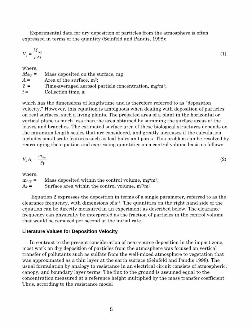
Experimental data for dry deposition of particles from the atmosphere is often expressed in terms of the quantity (Seinfeld and Pandis, 1998):
Vd =Mdep
c At (1)
where, Mdep = Mass deposited on the surface, mg A = Area of the surface, m2; c = Time-averaged aerosol particle concentration, mg/m3; t = Collection time, s;
which has the dimensions of length/time and is therefore referred to as "deposition velocity." However, this equation is ambiguous when dealing with deposition of particles on real surfaces, such a living plants. The projected area of a plant in the horizontal or vertical plane is much less than the area obtained by summing the surface areas of the leaves and branches. The estimated surface area of these biological structures depends on the minimum length scales that are considered, and greatly increases if the calculation includes small scale features such as leaf hairs and pores. This problem can be resolved by rearranging the equation and expressing quantities on a control volume basis as follows:
tcm
AV depvd = (2)
where, mdep = Mass deposited within the control volume, mg/m3; Av = Surface area within the control volume, m2/m3.
Equation 2 expresses the deposition in terms of a single parameter, referred to as the clearance frequency, with dimensions of s-1. The quantities on the right hand side of the equation can be directly measured in an experiment as described below. The clearance frequency can physically be interpreted as the fraction of particles in the control volume that would be removed per second at the initial rate.
Literature Values for Deposition Velocity
In contrast to the present consideration of near-source deposition in the impact zone, most work on dry deposition of particles from the atmosphere was focused on vertical transfer of pollutants such as sulfate from the well-mixed atmosphere to vegetation that was approximated as a thin layer at the earth surface (Seinfeld and Pandis 1998). The usual formulation by analogy to resistance in an electrical circuit consists of atmospheric, canopy, and boundary layer terms. The flux to the ground is assumed equal to the concentration measured at a reference height multiplied by the mass transfer coefficient. Thus, according to the resistance model
5
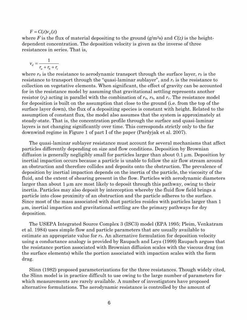
F = C(z)vd (z) where F is the flux of material depositing to the ground (g/m2s) and C(z) is the height-dependent concentration. The deposition velocity is given as the inverse of three resistances in series. That is,
cbad rrr
v++
=1
where ra is the resistance to aerodynamic transport through the surface layer, rb is the resistance to transport through the “quasi-laminar sublayer”, and rc is the resistance to collection on vegetative elements. When significant, the effect of gravity can be accounted for in the resistance model by assuming that gravitational settling represents another resistor (rg) acting in parallel with the combination of ra, rb, and rc. The resistance model for deposition is built on the assumption that close to the ground (i.e. from the top of the surface layer down), the flux of a depositing species is constant with height. Related to the assumption of constant flux, the model also assumes that the system is approximately at steady-state. That is, the concentration profile through the surface and quasi-laminar layers is not changing significantly over time. This corresponds strictly only to the far downwind regime in Figure 1 of part I of the paper (Pardyjak et al. 2007).
The quasi-laminar sublayer resistance must account for several mechanisms that affect particles differently depending on size and flow conditions. Deposition by Brownian diffusion is generally negligibly small for particles larger than about 0.1 μm. Deposition by inertial impaction occurs because a particle is unable to follow the air flow stream around an obstruction and therefore collides and deposits onto the obstruction. The prevalence of deposition by inertial impaction depends on the inertia of the particle, the viscosity of the fluid, and the extent of shearing present in the flow. Particles with aerodynamic diameters larger than about 1 μm are most likely to deposit through this pathway, owing to their inertia. Particles may also deposit by interception whereby the fluid flow field brings a particle into close proximity of an obstruction and the particle adheres to the surface. Since most of the mass associated with dust particles resides with particles larger than 1 μm, inertial impaction and gravitational settling are the primary pathways for dry deposition.
The USEPA Integrated Source Complex 3 (ISC3) model (EPA 1995; Pleim, Venkatram et al. 1984) uses simple flow and particle parameters that are usually available to estimate an appropriate value for rb. An alternative formulation for deposition velocity using a conductance analogy is provided by Raupach and Leys (1999) Raupach argues that the resistance portion associated with Brownian diffusion scales with the viscous drag (on the surface elements) while the portion associated with impaction scales with the form drag.
Slinn (1982) proposed parameterizations for the three resistances. Though widely cited, the Slinn model is in practice difficult to use owing to the large number of parameters for which measurements are rarely available. A number of investigators have proposed alternative formulations. The aerodynamic resistance is controlled by the amount of
6
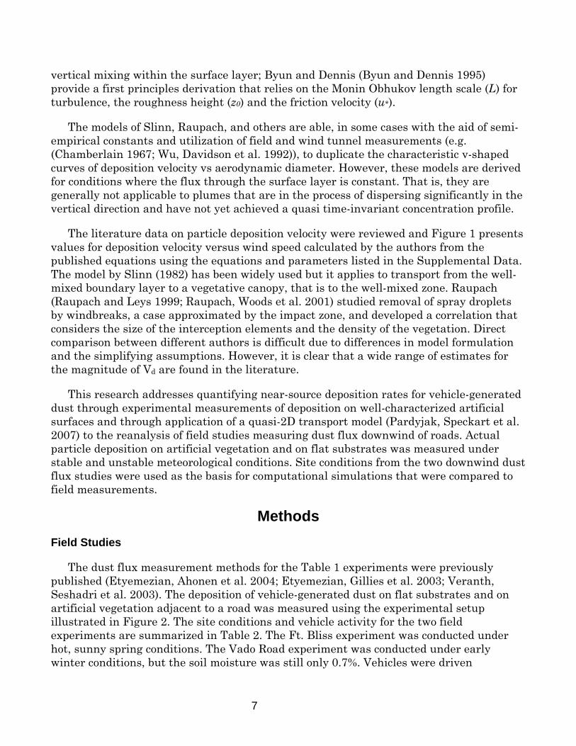
vertical mixing within the surface layer; Byun and Dennis (Byun and Dennis 1995) provide a first principles derivation that relies on the Monin Obhukov length scale (L) for turbulence, the roughness height (z0) and the friction velocity (u*).
The models of Slinn, Raupach, and others are able, in some cases with the aid of semi-empirical constants and utilization of field and wind tunnel measurements (e.g. (Chamberlain 1967; Wu, Davidson et al. 1992)), to duplicate the characteristic v-shaped curves of deposition velocity vs aerodynamic diameter. However, these models are derived for conditions where the flux through the surface layer is constant. That is, they are generally not applicable to plumes that are in the process of dispersing significantly in the vertical direction and have not yet achieved a quasi time-invariant concentration profile.
The literature data on particle deposition velocity were reviewed and Figure 1 presents values for deposition velocity versus wind speed calculated by the authors from the published equations using the equations and parameters listed in the Supplemental Data. The model by Slinn (1982) has been widely used but it applies to transport from the well-mixed boundary layer to a vegetative canopy, that is to the well-mixed zone. Raupach (Raupach and Leys 1999; Raupach, Woods et al. 2001) studied removal of spray droplets by windbreaks, a case approximated by the impact zone, and developed a correlation that considers the size of the interception elements and the density of the vegetation. Direct comparison between different authors is difficult due to differences in model formulation and the simplifying assumptions. However, it is clear that a wide range of estimates for the magnitude of Vd are found in the literature.
This research addresses quantifying near-source deposition rates for vehicle-generated dust through experimental measurements of deposition on well-characterized artificial surfaces and through application of a quasi-2D transport model (Pardyjak, Speckart et al. 2007) to the reanalysis of field studies measuring dust flux downwind of roads. Actual particle deposition on artificial vegetation and on flat substrates was measured under stable and unstable meteorological conditions. Site conditions from the two downwind dust flux studies were used as the basis for computational simulations that were compared to field measurements.
Methods Field Studies
The dust flux measurement methods for the Table 1 experiments were previously published (Etyemezian, Ahonen et al. 2004; Etyemezian, Gillies et al. 2003; Veranth, Seshadri et al. 2003). The deposition of vehicle-generated dust on flat substrates and on artificial vegetation adjacent to a road was measured using the experimental setup illustrated in Figure 2. The site conditions and vehicle activity for the two field experiments are summarized in Table 2. The Ft. Bliss experiment was conducted under hot, sunny spring conditions. The Vado Road experiment was conducted under early winter conditions, but the soil moisture was still only 0.7%. Vehicles were driven
7
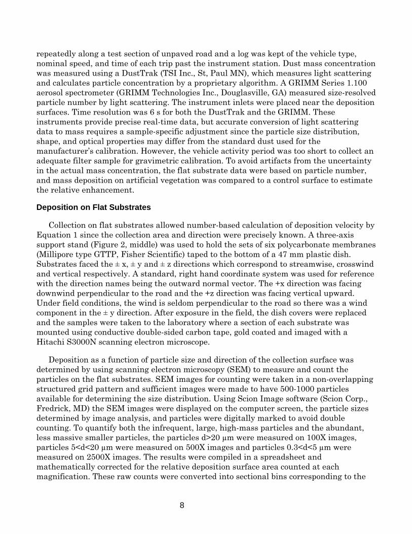
repeatedly along a test section of unpaved road and a log was kept of the vehicle type, nominal speed, and time of each trip past the instrument station. Dust mass concentration was measured using a DustTrak (TSI Inc., St, Paul MN), which measures light scattering and calculates particle concentration by a proprietary algorithm. A GRIMM Series 1.100 aerosol spectrometer (GRIMM Technologies Inc., Douglasville, GA) measured size-resolved particle number by light scattering. The instrument inlets were placed near the deposition surfaces. Time resolution was 6 s for both the DustTrak and the GRIMM. These instruments provide precise real-time data, but accurate conversion of light scattering data to mass requires a sample-specific adjustment since the particle size distribution, shape, and optical properties may differ from the standard dust used for the manufacturer’s calibration. However, the vehicle activity period was too short to collect an adequate filter sample for gravimetric calibration. To avoid artifacts from the uncertainty in the actual mass concentration, the flat substrate data were based on particle number, and mass deposition on artificial vegetation was compared to a control surface to estimate the relative enhancement.
Deposition on Flat Substrates
Collection on flat substrates allowed number-based calculation of deposition velocity by Equation 1 since the collection area and direction were precisely known. A three-axis support stand (Figure 2, middle) was used to hold the sets of six polycarbonate membranes (Millipore type GTTP, Fisher Scientific) taped to the bottom of a 47 mm plastic dish. Substrates faced the ± x, ± y and ± z directions which correspond to streamwise, crosswind and vertical respectively. A standard, right hand coordinate system was used for reference with the direction names being the outward normal vector. The +x direction was facing downwind perpendicular to the road and the +z direction was facing vertical upward. Under field conditions, the wind is seldom perpendicular to the road so there was a wind component in the ± y direction. After exposure in the field, the dish covers were replaced and the samples were taken to the laboratory where a section of each substrate was mounted using conductive double-sided carbon tape, gold coated and imaged with a Hitachi S3000N scanning electron microscope.
Deposition as a function of particle size and direction of the collection surface was determined by using scanning electron microscopy (SEM) to measure and count the particles on the flat substrates. SEM images for counting were taken in a non-overlapping structured grid pattern and sufficient images were made to have 500-1000 particles available for determining the size distribution. Using Scion Image software (Scion Corp., Fredrick, MD) the SEM images were displayed on the computer screen, the particle sizes determined by image analysis, and particles were digitally marked to avoid double counting. To quantify both the infrequent, large, high-mass particles and the abundant, less massive smaller particles, the particles d>20 µm were measured on 100X images, particles 5<d<20 µm were measured on 500X images and particles 0.3<d<5 µm were measured on 2500X images. The results were compiled in a spreadsheet and mathematically corrected for the relative deposition surface area counted at each magnification. These raw counts were converted into sectional bins corresponding to the
8
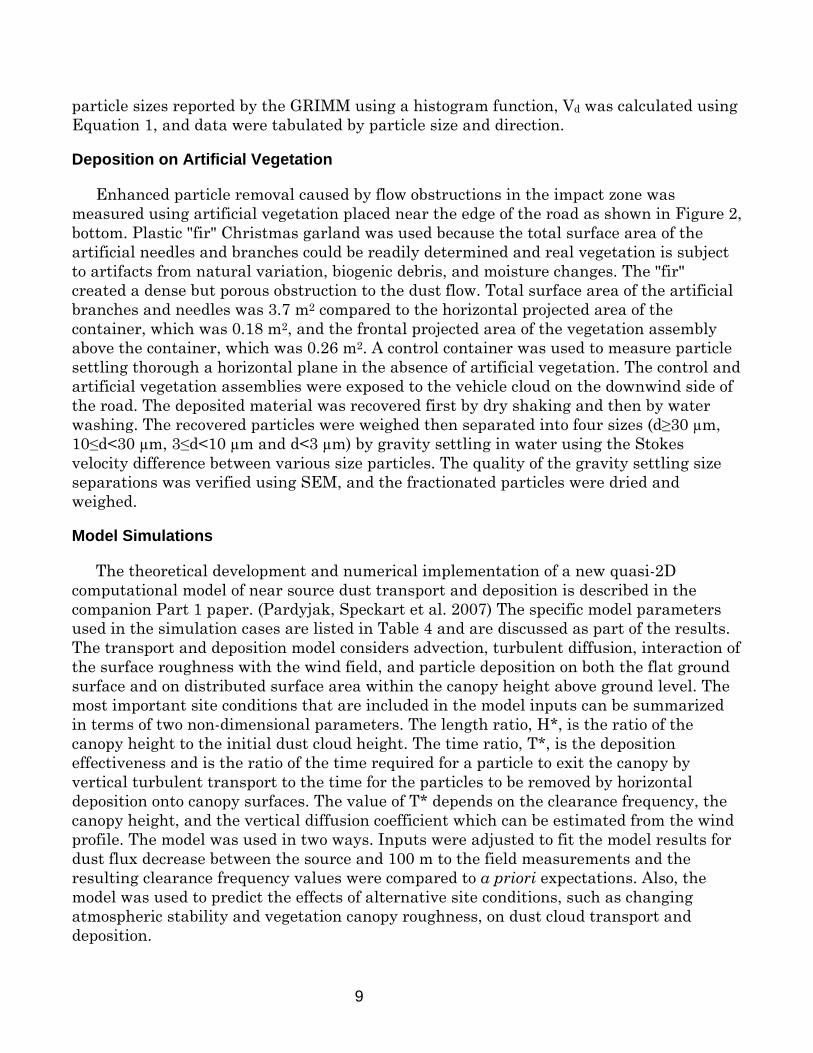
particle sizes reported by the GRIMM using a histogram function, Vd was calculated using Equation 1, and data were tabulated by particle size and direction.
Deposition on Artificial Vegetation
Enhanced particle removal caused by flow obstructions in the impact zone was measured using artificial vegetation placed near the edge of the road as shown in Figure 2, bottom. Plastic "fir" Christmas garland was used because the total surface area of the artificial needles and branches could be readily determined and real vegetation is subject to artifacts from natural variation, biogenic debris, and moisture changes. The "fir" created a dense but porous obstruction to the dust flow. Total surface area of the artificial branches and needles was 3.7 m2 compared to the horizontal projected area of the container, which was 0.18 m2, and the frontal projected area of the vegetation assembly above the container, which was 0.26 m2. A control container was used to measure particle settling thorough a horizontal plane in the absence of artificial vegetation. The control and artificial vegetation assemblies were exposed to the vehicle cloud on the downwind side of the road. The deposited material was recovered first by dry shaking and then by water washing. The recovered particles were weighed then separated into four sizes (d≥30 µm, 10≤d<30 µm, 3≤d<10 µm and d<3 µm) by gravity settling in water using the Stokes velocity difference between various size particles. The quality of the gravity settling size separations was verified using SEM, and the fractionated particles were dried and weighed.
Model Simulations
The theoretical development and numerical implementation of a new quasi-2D computational model of near source dust transport and deposition is described in the companion Part 1 paper. (Pardyjak, Speckart et al. 2007) The specific model parameters used in the simulation cases are listed in Table 4 and are discussed as part of the results. The transport and deposition model considers advection, turbulent diffusion, interaction of the surface roughness with the wind field, and particle deposition on both the flat ground surface and on distributed surface area within the canopy height above ground level. The most important site conditions that are included in the model inputs can be summarized in terms of two non-dimensional parameters. The length ratio, H*, is the ratio of the canopy height to the initial dust cloud height. The time ratio, T*, is the deposition effectiveness and is the ratio of the time required for a particle to exit the canopy by vertical turbulent transport to the time for the particles to be removed by horizontal deposition onto canopy surfaces. The value of T* depends on the clearance frequency, the canopy height, and the vertical diffusion coefficient which can be estimated from the wind profile. The model was used in two ways. Inputs were adjusted to fit the model results for dust flux decrease between the source and 100 m to the field measurements and the resulting clearance frequency values were compared to a priori expectations. Also, the model was used to predict the effects of alternative site conditions, such as changing atmospheric stability and vegetation canopy roughness, on dust cloud transport and deposition.
9
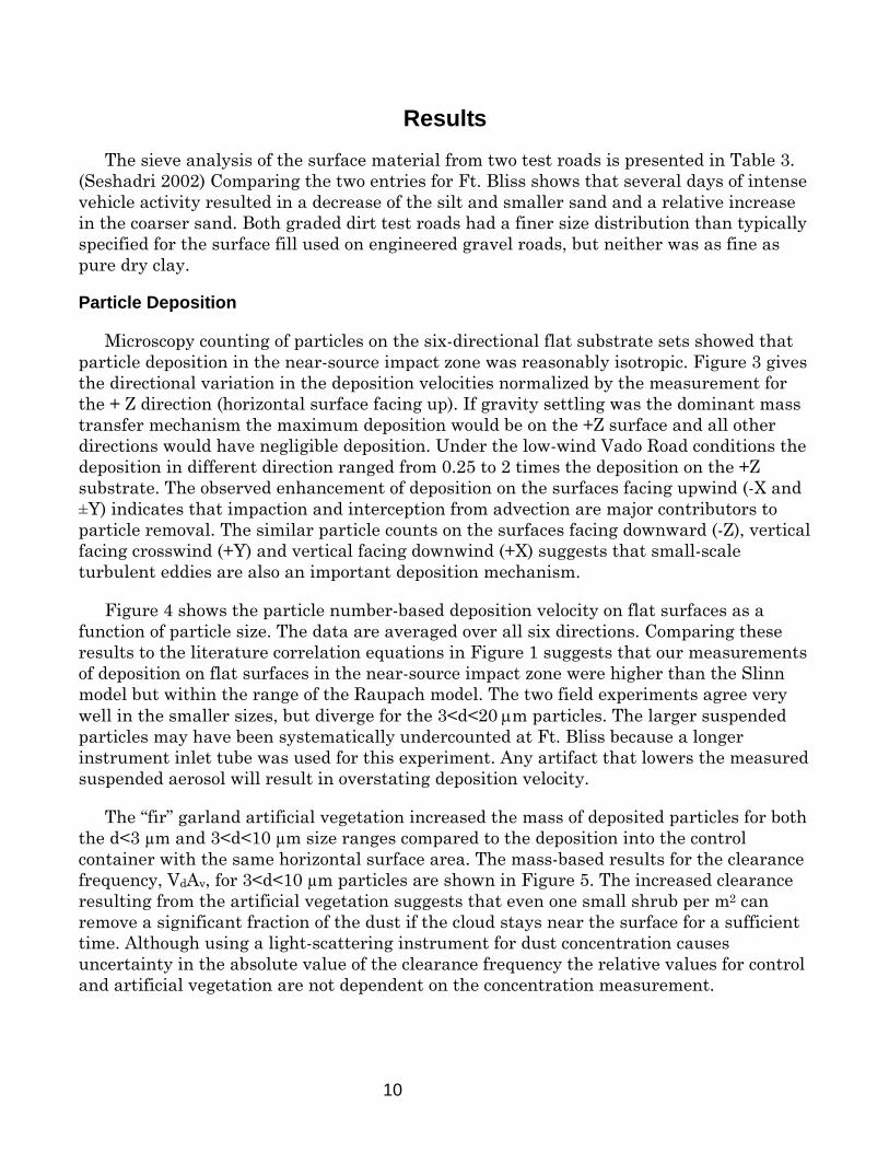
Results The sieve analysis of the surface material from two test roads is presented in Table 3.
(Seshadri 2002) Comparing the two entries for Ft. Bliss shows that several days of intense vehicle activity resulted in a decrease of the silt and smaller sand and a relative increase in the coarser sand. Both graded dirt test roads had a finer size distribution than typically specified for the surface fill used on engineered gravel roads, but neither was as fine as pure dry clay.
Particle Deposition
Microscopy counting of particles on the six-directional flat substrate sets showed that particle deposition in the near-source impact zone was reasonably isotropic. Figure 3 gives the directional variation in the deposition velocities normalized by the measurement for the + Z direction (horizontal surface facing up). If gravity settling was the dominant mass transfer mechanism the maximum deposition would be on the +Z surface and all other directions would have negligible deposition. Under the low-wind Vado Road conditions the deposition in different direction ranged from 0.25 to 2 times the deposition on the +Z substrate. The observed enhancement of deposition on the surfaces facing upwind (-X and ±Y) indicates that impaction and interception from advection are major contributors to particle removal. The similar particle counts on the surfaces facing downward (-Z), vertical facing crosswind (+Y) and vertical facing downwind (+X) suggests that small-scale turbulent eddies are also an important deposition mechanism.
Figure 4 shows the particle number-based deposition velocity on flat surfaces as a function of particle size. The data are averaged over all six directions. Comparing these results to the literature correlation equations in Figure 1 suggests that our measurements of deposition on flat surfaces in the near-source impact zone were higher than the Slinn model but within the range of the Raupach model. The two field experiments agree very well in the smaller sizes, but diverge for the 3<d<20 μm particles. The larger suspended particles may have been systematically undercounted at Ft. Bliss because a longer instrument inlet tube was used for this experiment. Any artifact that lowers the measured suspended aerosol will result in overstating deposition velocity.
The “fir” garland artificial vegetation increased the mass of deposited particles for both the d<3 µm and 3<d<10 µm size ranges compared to the deposition into the control container with the same horizontal surface area. The mass-based results for the clearance frequency, VdAv, for 3<d<10 µm particles are shown in Figure 5. The increased clearance resulting from the artificial vegetation suggests that even one small shrub per m2 can remove a significant fraction of the dust if the cloud stays near the surface for a sufficient time. Although using a light-scattering instrument for dust concentration causes uncertainty in the absolute value of the clearance frequency the relative values for control and artificial vegetation are not dependent on the concentration measurement.
10
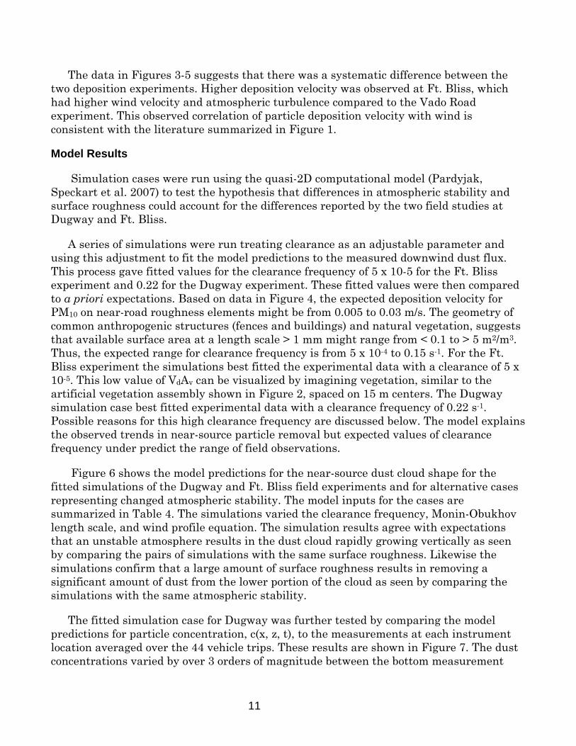
The data in Figures 3-5 suggests that there was a systematic difference between the two deposition experiments. Higher deposition velocity was observed at Ft. Bliss, which had higher wind velocity and atmospheric turbulence compared to the Vado Road experiment. This observed correlation of particle deposition velocity with wind is consistent with the literature summarized in Figure 1.
Model Results
Simulation cases were run using the quasi-2D computational model (Pardyjak, Speckart et al. 2007) to test the hypothesis that differences in atmospheric stability and surface roughness could account for the differences reported by the two field studies at Dugway and Ft. Bliss.
A series of simulations were run treating clearance as an adjustable parameter and using this adjustment to fit the model predictions to the measured downwind dust flux. This process gave fitted values for the clearance frequency of 5 x 10⁻⁵ for the Ft. Bliss experiment and 0.22 for the Dugway experiment. These fitted values were then compared to a priori expectations. Based on data in Figure 4, the expected deposition velocity for PM10 on near-road roughness elements might be from 0.005 to 0.03 m/s. The geometry of common anthropogenic structures (fences and buildings) and natural vegetation, suggests that available surface area at a length scale > 1 mm might range from < 0.1 to > 5 m2/m3. Thus, the expected range for clearance frequency is from 5 x 10⁻⁴ to 0.15 s-1. For the Ft. Bliss experiment the simulations best fitted the experimental data with a clearance of 5 x 10⁻⁵. This low value of VdAv can be visualized by imagining vegetation, similar to the artificial vegetation assembly shown in Figure 2, spaced on 15 m centers. The Dugway simulation case best fitted experimental data with a clearance frequency of 0.22 s-1. Possible reasons for this high clearance frequency are discussed below. The model explains the observed trends in near-source particle removal but expected values of clearance frequency under predict the range of field observations.
Figure 6 shows the model predictions for the near-source dust cloud shape for the fitted simulations of the Dugway and Ft. Bliss field experiments and for alternative cases representing changed atmospheric stability. The model inputs for the cases are summarized in Table 4. The simulations varied the clearance frequency, Monin-Obukhov length scale, and wind profile equation. The simulation results agree with expectations that an unstable atmosphere results in the dust cloud rapidly growing vertically as seen by comparing the pairs of simulations with the same surface roughness. Likewise the simulations confirm that a large amount of surface roughness results in removing a significant amount of dust from the lower portion of the cloud as seen by comparing the simulations with the same atmospheric stability.
The fitted simulation case for Dugway was further tested by comparing the model predictions for particle concentration, c(x, z, t), to the measurements at each instrument location averaged over the 44 vehicle trips. These results are shown in Figure 7. The dust concentrations varied by over 3 orders of magnitude between the bottom measurement
11
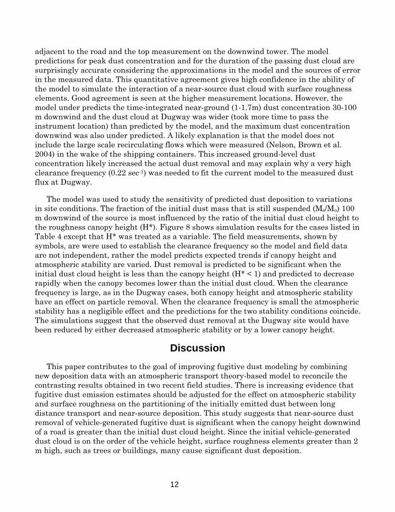
adjacent to the road and the top measurement on the downwind tower. The model predictions for peak dust concentration and for the duration of the passing dust cloud are surprisingly accurate considering the approximations in the model and the sources of error in the measured data. This quantitative agreement gives high confidence in the ability of the model to simulate the interaction of a near-source dust cloud with surface roughness elements. Good agreement is seen at the higher measurement locations. However, the model under predicts the time-integrated near-ground (1-1.7m) dust concentration 30-100 m downwind and the dust cloud at Dugway was wider (took more time to pass the instrument location) than predicted by the model, and the maximum dust concentration downwind was also under predicted. A likely explanation is that the model does not include the large scale recirculating flows which were measured (Nelson, Brown et al. 2004) in the wake of the shipping containers. This increased ground-level dust concentration likely increased the actual dust removal and may explain why a very high clearance frequency (0.22 sec-1) was needed to fit the current model to the measured dust flux at Dugway.
The model was used to study the sensitivity of predicted dust deposition to variations in site conditions. The fraction of the initial dust mass that is still suspended (Ms/Mo) 100 m downwind of the source is most influenced by the ratio of the initial dust cloud height to the roughness canopy height (H*). Figure 8 shows simulation results for the cases listed in Table 4 except that H* was treated as a variable. The field measurements, shown by symbols, are were used to establish the clearance frequency so the model and field data are not independent, rather the model predicts expected trends if canopy height and atmospheric stability are varied. Dust removal is predicted to be significant when the initial dust cloud height is less than the canopy height (H* < 1) and predicted to decrease rapidly when the canopy becomes lower than the initial dust cloud. When the clearance frequency is large, as in the Dugway cases, both canopy height and atmospheric stability have an effect on particle removal. When the clearance frequency is small the atmospheric stability has a negligible effect and the predictions for the two stability conditions coincide. The simulations suggest that the observed dust removal at the Dugway site would have been reduced by either decreased atmospheric stability or by a lower canopy height.
Discussion This paper contributes to the goal of improving fugitive dust modeling by combining
new deposition data with an atmospheric transport theory-based model to reconcile the contrasting results obtained in two recent field studies. There is increasing evidence that fugitive dust emission estimates should be adjusted for the effect on atmospheric stability and surface roughness on the partitioning of the initially emitted dust between long distance transport and near-source deposition. This study suggests that near-source dust removal of vehicle-generated fugitive dust is significant when the canopy height downwind of a road is greater than the initial dust cloud height. Since the initial vehicle-generated dust cloud is on the order of the vehicle height, surface roughness elements greater than 2 m high, such as trees or buildings, many cause significant dust deposition.
12
The methods used in this study to measure number-based particle deposition are labor intensive, but provide precise, time-resolved data. The data and methods demonstrated in this study can be used for future analysis of field data on horizontal dust flux and to design studies to better quantify the relationship between the configuration of near-ground surfaces and the removal of dust from vehicle-generated clouds. The measurement of particle concentration in the air is a source of uncertainty in the results since the same aerosol mechanisms causing particle deposition on vegetative surfaces also cause instrument inlet and line sampling losses. Our experimental measurements of particle deposition on flat surfaces gives deposition velocities that are an order of magnitude higher than are predicted by the Slinn equation (Slinn 1982), but that are within the range reported by Raupach (Raupach and Leys 1999; Raupach, Woods et al. 2001). The correlations and submodels presented in Figure 1 are simplifications that were derived for different limiting cases. Slinn studied vertical transport from the atmosphere to a horizontal area of forest canopy while the work of Raupach and the data from this study involve deposition from a horizontally moving cloud impinging on the projected area of a surface. Slinn reasoned that because momentum transfer from the wind to ground is higher over a forest, then downward particle transfer should also be higher, and developed a model that used the wind velocity profile in the forest canopy as a parameter. The experiments in this study are more closely analogous to the deposition predicted by models of single fiber filtration efficiency.
Using literature data for atmospheric flow and mixing inputs and using estimates of the clearance frequency that are consistent with experimental data, the quasi-2D model was able to partially explain the differences between the two field experiments that measured dust flux near and 100 m downwind of a road. As shown by Figures 6 and 8, differences in the canopy height, the clearance frequency, and the atmospheric stability account for the difference between <5% dust removal reported for Ft. Bliss and the 85% removal observed at Dugway. The highly simplified Gaussian dispersion model previously used by Etyemezian et al. (Etyemezian, Ahonen et al. 2004; Etyemezian, Gillies et al. 2003) fitted the field experimental data well for the low roughness and unstable atmosphere of the Ft. Bliss experiment but under predicted the measured dust removal for the Dugway experiment. The improved ability to match field measurements, including the detailed time-concentration curves shown in Figure 7, indicate that the new quasi-2D model is a significant improvement over previous computational studies of near-source dust cloud behavior, and that the model captures much of the important physics.
The artificial vegetation experiments demonstrated the usefulness of the technique, but had limitations. Based on Raupach’s results the density of “fir” garland used was higher than optimal for dust removal and this probably resulted in flow around rather than through the artificial vegetation. The effect of the collection container on the near-surface air-flow confounds results. An alternative apparatus design would have been to bury the collection container so the rim was flush with the ground surface, but this would have resulted in collecting large amounts of material moving along the ground by saltation, causing a different, and likely greater, artifact.
13

A major limitation of the current computational model is that there is no basis for predicting the clearance frequency (VdAv) a priori based on site descriptive data such as vegetation species or the spacing of constructed structures. Developing a submodel for predicting this parameter will require better understanding of small-scale fluid and particle flow dynamics combined with wind tunnel experimentation. Having theoretical or empirical values for clearance frequency under specific site conditions will contribute to the accuracy of regional-scale air quality models since the modeling techniques described in these companion papers can provide near-source deposition corrections for the current fugitive dust emission factors.
Acknowledgements
This work was supported by the Strategic Environmental Research and Development Program project SI-1190, Southwest Consortium for Environmental Research and Policy projects A-02-07, A-04-06, and A-05-05. John G. Watson provide seminal ideas and insights. Richard Countess provided detailed comments on a conference presentation of this work. The contributions of the many University of Texas at El Paso undergraduate students, graduate students Gauri Seshadri, Raed Labban, and Tom Booth, laboratory technician Erin Kaser, and collaborators Ernesto Alfaro-Moreno, Adrian Vasquez, John Walton, Jack Gillies, and Judith Chow are acknowledged.
14
References Byun, D. W. and R. Dennis (1995). “Design Artifacts in Eulerian Air Quality Models:
Evaluation of the Effects of Layer Thickness and Vertical Profile Correction on Surface Ozone Concentrations.” Atmospheric Environment 29: 105-126.
Chamberlain, A. C. (1967). “Transport of Lycopodium Spores and Other Small Particles
to Rough Surfaces.” Proceedings of the Royal Society of London, Series A Mathematical and Physical Sciences 296(1444): 45-60.
Code of Federal Regulations (2006). Code of Federal Regulations, 40CFR51 Subpart P -
Protection of Visibility. Government Printing Office, EPA (1995). User's Guide for the Industrial Source Complex (ISC3) Dispersion Models.
Volume II, Description of Algorithms. US Environmental Protection Agency, Office of Planning and Standards,
EPA (1998). AP-42, Chapter 13.2.2 Unpaved Roads. U.S. Environmental Protection
Agency, AP-42, Chapter 13.2.2 Unpaved Roads. Etyemezian, V., S. Ahonen, D. Nikolic, J. Gillies, H. Kuhns, D. Gillette and J. Veranth
(2004). “Dust deposition and removal in the arid southwestern United States: measurements and model results.” Journal of the Air & Waste Management Association 54: 1099-1111.
Etyemezian, V., J. Gillies, H. Kuhns, D. Nikolic, J. Watson, J. Veranth, R. Labban, G.
Seshadri and D. Gillette (2003). Field Testing and Evaluation of Dust Deposition and Removal Mechanisms: Final Report. Western States Air Resources Council (WESTAR),
Nelson, M. A., M. J. Brown, E. R. Pardyjak and J. C. Klewicki (2004). Area averaged
profiles over the mock urban setting test array. Fifth Conference on the Urban Environment, American Meteorological Society, 15.2.
Pardyjak, E. R., S. O. Speckart, F. Yin and J. M. Veranth (2007). “Near-source
deposition of vehicle generated fugitive dust on vegetation and buildings. Part 1: Model development and theory.” In Preparation:
Pleim, J., A. Venkatram and R. Yamartino (1984). ADOM/TADAP Model Development
Program. Volume 4. The Dry Deposition Module. Ontario Ministry of the Environment, Rexdale, Ontario,
15
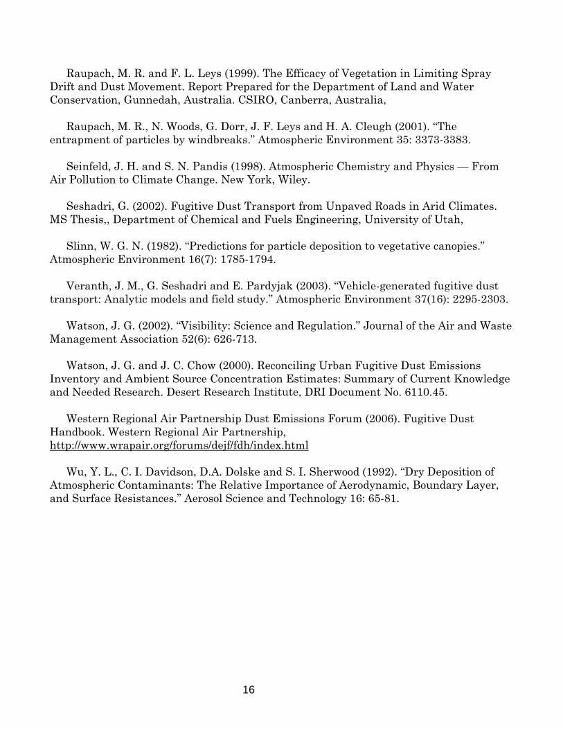
Raupach, M. R. and F. L. Leys (1999). The Efficacy of Vegetation in Limiting Spray Drift and Dust Movement. Report Prepared for the Department of Land and Water Conservation, Gunnedah, Australia. CSIRO, Canberra, Australia,
Raupach, M. R., N. Woods, G. Dorr, J. F. Leys and H. A. Cleugh (2001). “The
entrapment of particles by windbreaks.” Atmospheric Environment 35: 3373-3383. Seinfeld, J. H. and S. N. Pandis (1998). Atmospheric Chemistry and Physics — From
Air Pollution to Climate Change. New York, Wiley. Seshadri, G. (2002). Fugitive Dust Transport from Unpaved Roads in Arid Climates.
MS Thesis,, Department of Chemical and Fuels Engineering, University of Utah, Slinn, W. G. N. (1982). “Predictions for particle deposition to vegetative canopies.”
Atmospheric Environment 16(7): 1785-1794. Veranth, J. M., G. Seshadri and E. Pardyjak (2003). “Vehicle-generated fugitive dust
transport: Analytic models and field study.” Atmospheric Environment 37(16): 2295-2303. Watson, J. G. (2002). “Visibility: Science and Regulation.” Journal of the Air and Waste
Management Association 52(6): 626-713. Watson, J. G. and J. C. Chow (2000). Reconciling Urban Fugitive Dust Emissions
Inventory and Ambient Source Concentration Estimates: Summary of Current Knowledge and Needed Research. Desert Research Institute, DRI Document No. 6110.45.
Western Regional Air Partnership Dust Emissions Forum (2006). Fugitive Dust
Handbook. Western Regional Air Partnership, http://www.wrapair.org/forums/dejf/fdh/index.html
Wu, Y. L., C. I. Davidson, D.A. Dolske and S. I. Sherwood (1992). “Dry Deposition of
Atmospheric Contaminants: The Relative Importance of Aerodynamic, Boundary Layer, and Surface Resistances.” Aerosol Science and Technology 16: 65-81.
16
Tables
Flux Measurement Experiment
Dugway Ft. Bliss
Citation [Veranth, 2003 #1350] [Etyemezian, 2004 #1414; Etyemezian, 2003 #1377]
Location UTM Coordinates
Northwestern Utah Zone 12 3 14 800 E 44 53 100 N
West Texas Zone 13 3 70 500 E 35 28 100 N
Month September 2001 April 2002
Time of Day Night Afternoon
Atmospheric Stability Neutral-Stable Unstable
Surface Roughness 2.5 x 2.5 x 8 m shipping containers simulating buildings
Small sand dunes with sparse 0.1-0.3 m brush
Dust Flux Change 85% decrease < 5% decrease
Table 1. Published field measurements of dust flux downwind of a test road.
Figures and Tables 16
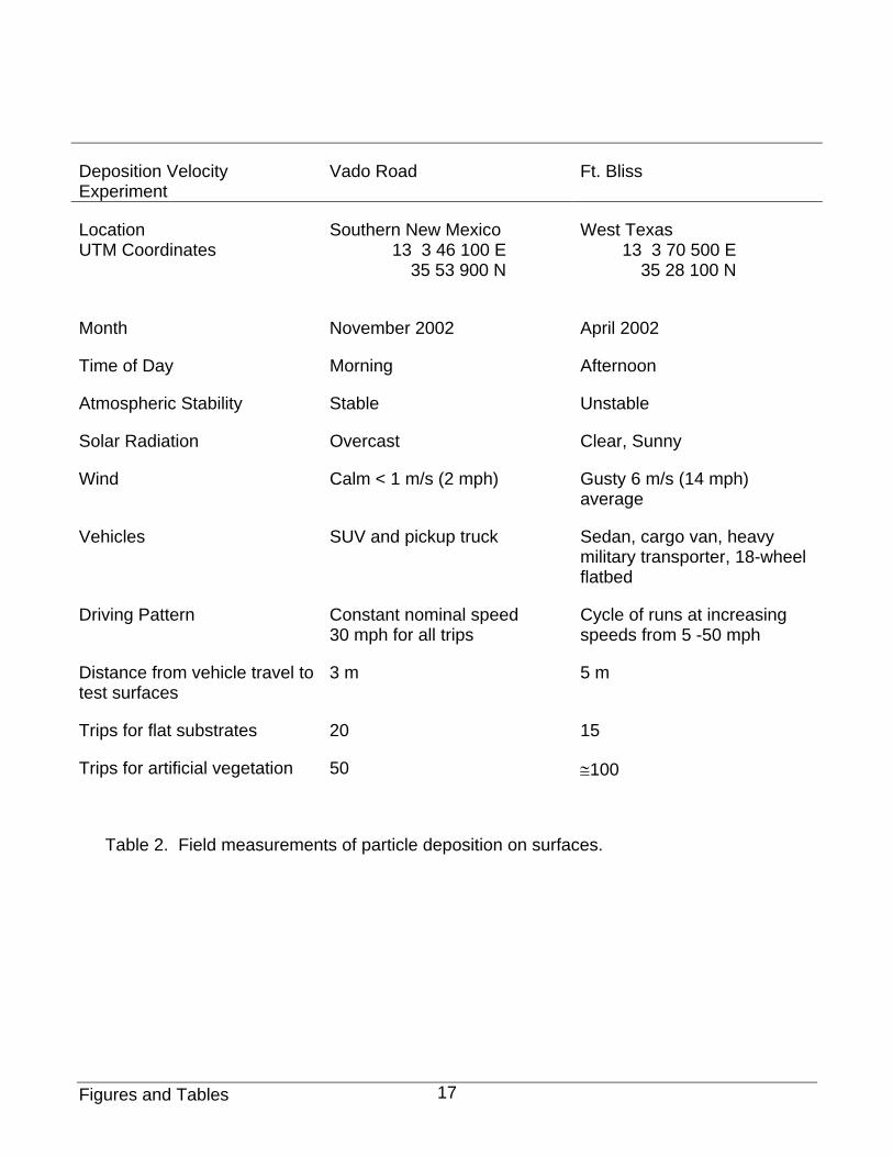
Deposition Velocity Experiment
Vado Road Ft. Bliss
Location UTM Coordinates
Southern New Mexico 13 3 46 100 E 35 53 900 N
West Texas 13 3 70 500 E 35 28 100 N
Month November 2002 April 2002
Time of Day Morning Afternoon
Atmospheric Stability Stable Unstable
Solar Radiation Overcast Clear, Sunny
Wind Calm < 1 m/s (2 mph) Gusty 6 m/s (14 mph) average
Vehicles SUV and pickup truck Sedan, cargo van, heavy military transporter, 18-wheel flatbed
Driving Pattern Constant nominal speed 30 mph for all trips
Cycle of runs at increasing speeds from 5 -50 mph
Distance from vehicle travel to test surfaces
3 m 5 m
Trips for flat substrates 20 15
Trips for artificial vegetation 50 ≅100
Table 2. Field measurements of particle deposition on surfaces.
Figures and Tables 17
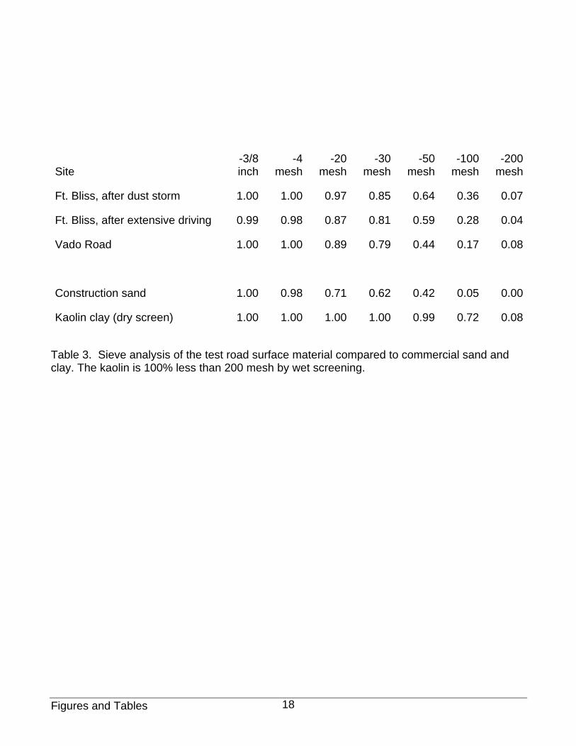
Site -3/8 inch
-4 mesh
-20 mesh
-30 mesh
-50 mesh
-100 mesh
-200 mesh
Ft. Bliss, after dust storm 1.00 1.00 0.97 0.85 0.64 0.36 0.07
Ft. Bliss, after extensive driving 0.99 0.98 0.87 0.81 0.59 0.28 0.04
Vado Road 1.00 1.00 0.89 0.79 0.44 0.17 0.08
Construction sand 1.00 0.98 0.71 0.62 0.42 0.05 0.00
Kaolin clay (dry screen) 1.00 1.00 1.00 1.00 0.99 0.72 0.08
Table 3. Sieve analysis of the test road surface material compared to commercial sand and clay. The kaolin is 100% less than 200 mesh by wet screening.
Figures and Tables 18
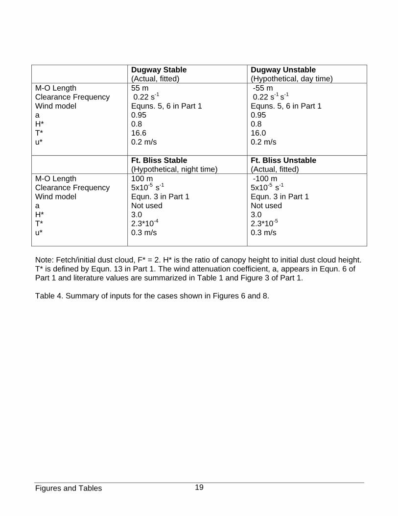
Dugway Stable
(Actual, fitted) Dugway Unstable (Hypothetical, day time)
M-O Length Clearance Frequency Wind model a H* T* u*
55 m 0.22 s-1
Equns. 5, 6 in Part 1 0.95 0.8 16.6 0.2 m/s
-55 m 0.22 s-1 s-1
Equns. 5, 6 in Part 1 0.95 0.8 16.0 0.2 m/s
Ft. Bliss Stable (Hypothetical, night time)
Ft. Bliss Unstable (Actual, fitted)
M-O Length Clearance Frequency Wind model a H* T* u*
100 m 5x10⁻⁵ s-1
Equn. 3 in Part 1 Not used 3.0 2.3*10-4
0.3 m/s
-100 m 5x10⁻⁵ s-1
Equn. 3 in Part 1 Not used 3.0 2.3*10-5
0.3 m/s
Note: Fetch/initial dust cloud, F* = 2. H* is the ratio of canopy height to initial dust cloud height. T* is defined by Equn. 13 in Part 1. The wind attenuation coefficient, a, appears in Equn. 6 of Part 1 and literature values are summarized in Table 1 and Figure 3 of Part 1. Table 4. Summary of inputs for the cases shown in Figures 6 and 8.
Figures and Tables 19
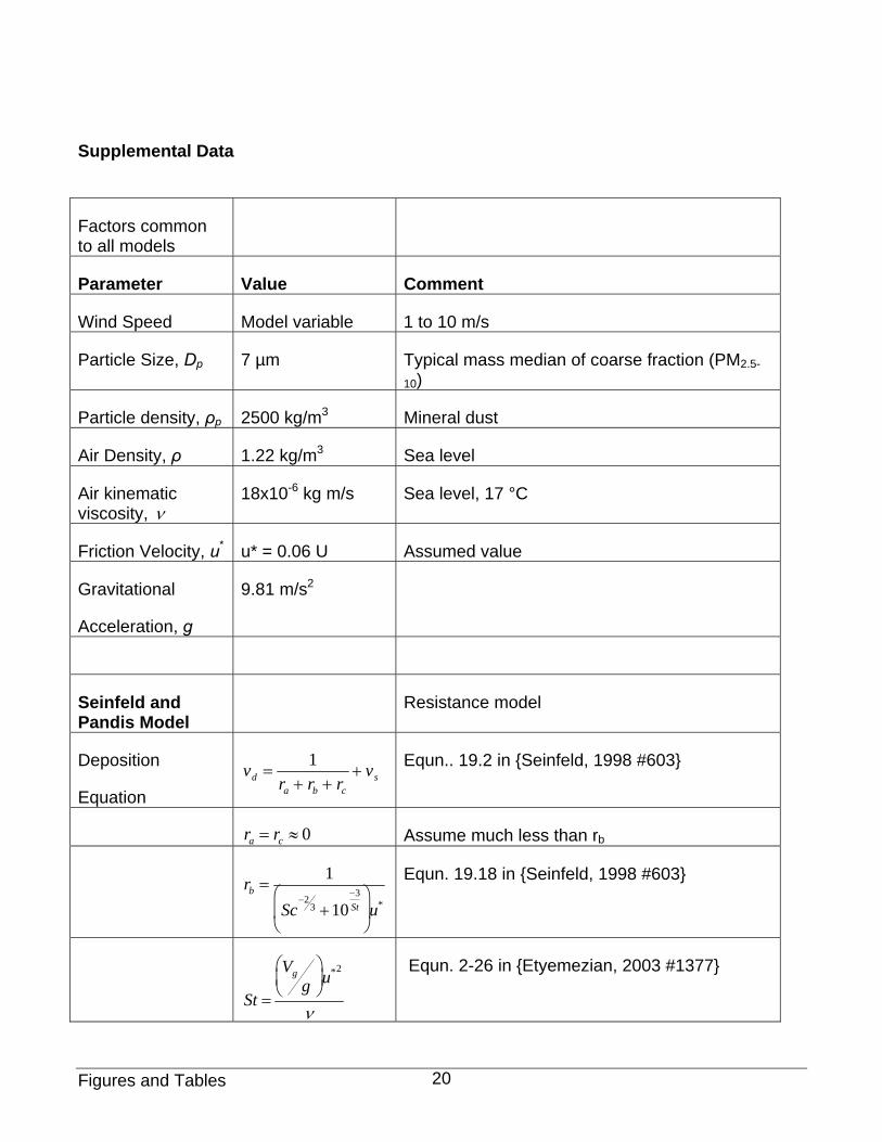
Supplemental Data
Factors common to all models
Parameter Value Comment
Wind Speed Model variable 1 to 10 m/s
Particle Size, Dp 7 µm Typical mass median of coarse fraction (PM2.5-
10)
Particle density, ρp 2500 kg/m3 Mineral dust
Air Density, ρ 1.22 kg/m3 Sea level
Air kinematic viscosity, ν
18x10-6 kg m/s Sea level, 17 °C
Friction Velocity, u* u* = 0.06 U Assumed value
Gravitational
Acceleration, g
9.81 m/s2
Seinfeld and Pandis Model
Resistance model
Deposition
Equation vd =
1ra + rb + rc
+ vs Equn.. 19.2 in {Seinfeld, 1998 #603}
ra = rc ≈ 0 Assume much less than rb
rb =1
Sc−2
3 +10−3St
⎛
⎝ ⎜
⎞
⎠ ⎟ u*
Equn. 19.18 in {Seinfeld, 1998 #603}
St =
Vgg
⎛ ⎝ ⎜
⎞ ⎠ ⎟ u*2
ν
Equn. 2-26 in {Etyemezian, 2003 #1377}
Figures and Tables 20
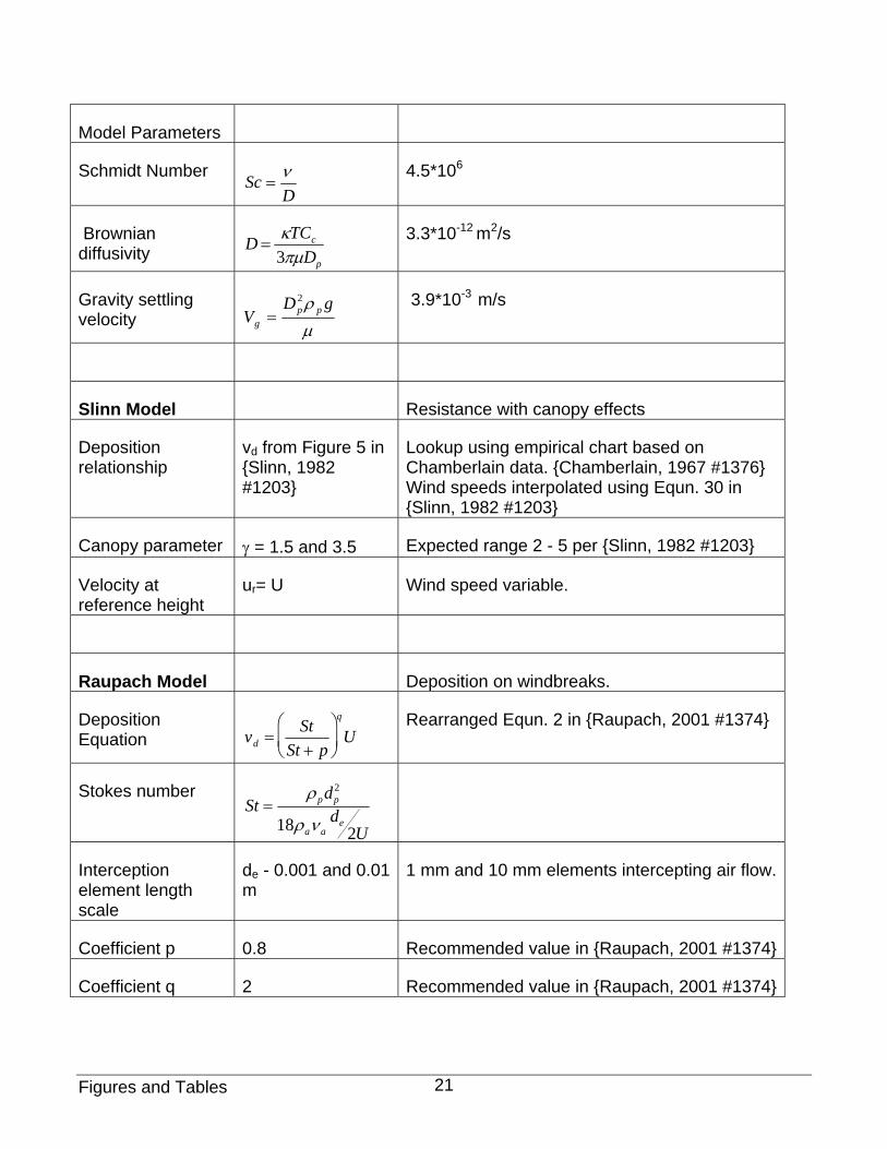
Model Parameters
Schmidt Number D
Sc ν= 4.5*106
Brownian diffusivity D =
κTCc
3πμDp
3.3*10-12 m2/s
Gravity settling velocity μ
ρ gDV pp
g
2
= 3.9*10-3 m/s
Slinn Model Resistance with canopy effects
Deposition relationship
vd from Figure 5 in {Slinn, 1982 #1203}
Lookup using empirical chart based on Chamberlain data. {Chamberlain, 1967 #1376} Wind speeds interpolated using Equn. 30 in {Slinn, 1982 #1203}
Canopy parameter γ = 1.5 and 3.5 Expected range 2 - 5 per {Slinn, 1982 #1203}
Velocity at reference height
ur= U Wind speed variable.
Raupach Model Deposition on windbreaks.
Deposition Equation vd =
StSt + p
⎛
⎝ ⎜
⎞
⎠ ⎟
q
U Rearranged Equn. 2 in {Raupach, 2001 #1374}
Stokes number St =
ρpdp2
18ρaν ade
2U
Interception element length scale
de - 0.001 and 0.01 m
1 mm and 10 mm elements intercepting air flow.
Coefficient p 0.8 Recommended value in {Raupach, 2001 #1374}
Coefficient q 2 Recommended value in {Raupach, 2001 #1374}
Figures and Tables 21

Supplemental Table 1. Model citations, equations, and parameters used by the authors to calculate deposition velocity versus wind speed in Figure 2.
Figures and Tables 22
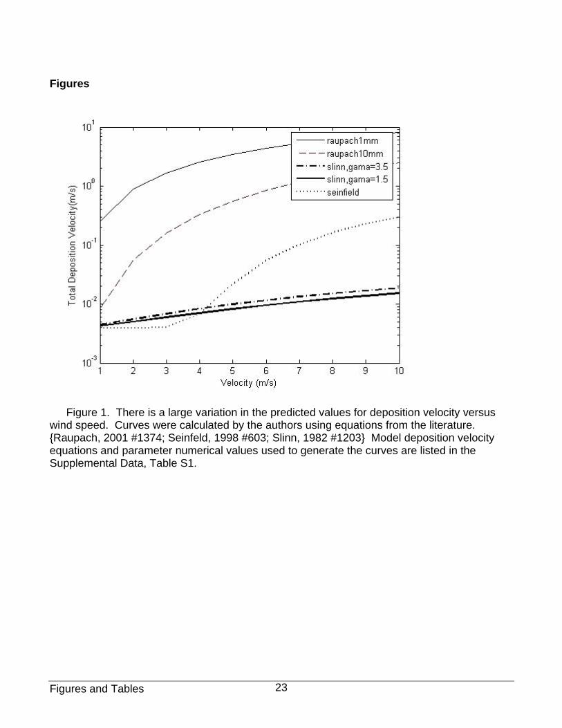
Figures
Figure 1. There is a large variation in the predicted values for deposition velocity versus wind speed. Curves were calculated by the authors using equations from the literature. {Raupach, 2001 #1374; Seinfeld, 1998 #603; Slinn, 1982 #1203} Model deposition velocity equations and parameter numerical values used to generate the curves are listed in the Supplemental Data, Table S1.
Figures and Tables 23
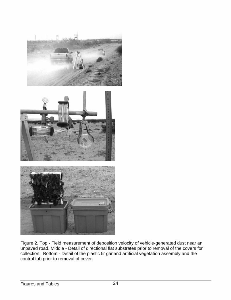
Figure 2. Top - Field measurement of deposition velocity of vehicle-generated dust near an unpaved road. Middle - Detail of directional flat substrates prior to removal of the covers for collection. Bottom - Detail of the plastic fir garland artificial vegetation assembly and the control tub prior to removal of cover.
Figures and Tables 24
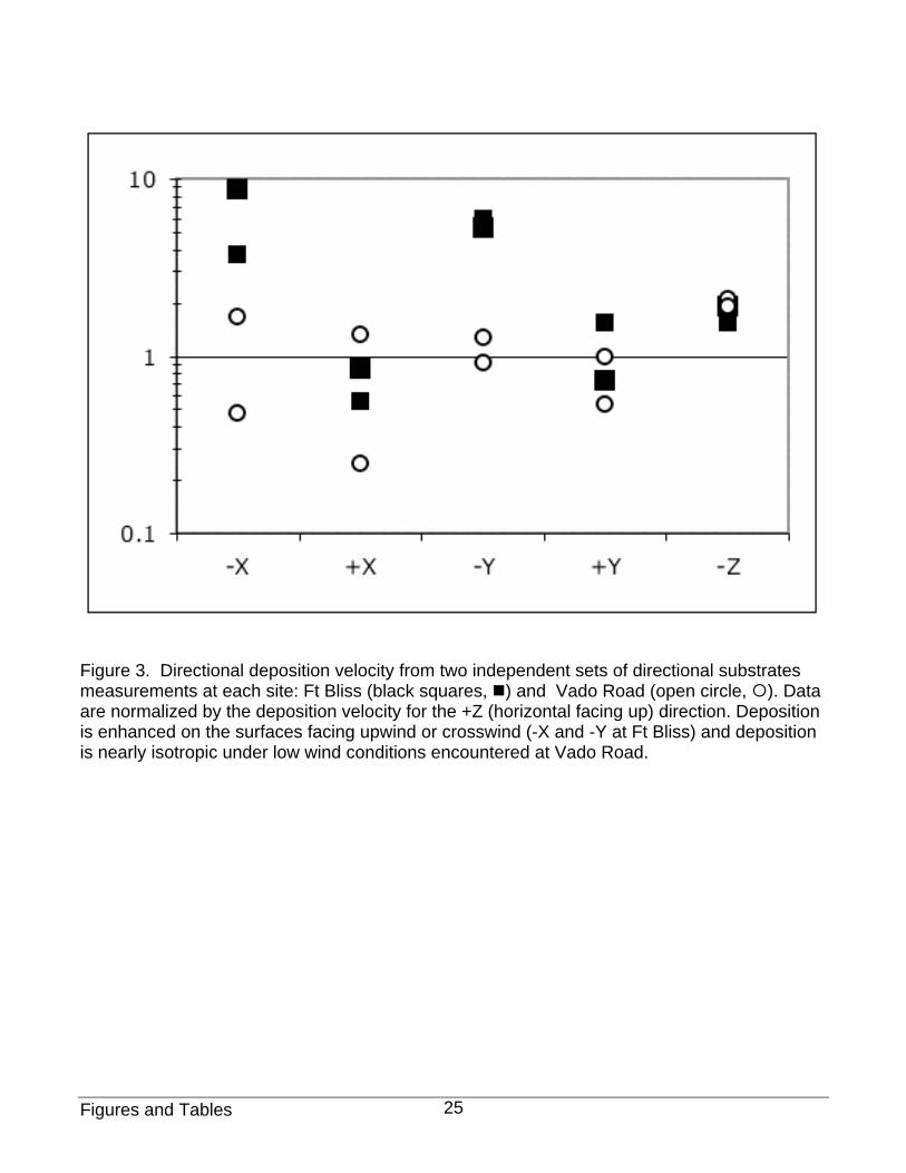
Figure 3. Directional deposition velocity from two independent sets of directional substrates measurements at each site: Ft Bliss (black squares, ) and Vado Road (open circle, ). Data are normalized by the deposition velocity for the +Z (horizontal facing up) direction. Deposition is enhanced on the surfaces facing upwind or crosswind (-X and -Y at Ft Bliss) and deposition is nearly isotropic under low wind conditions encountered at Vado Road.
Figures and Tables 25
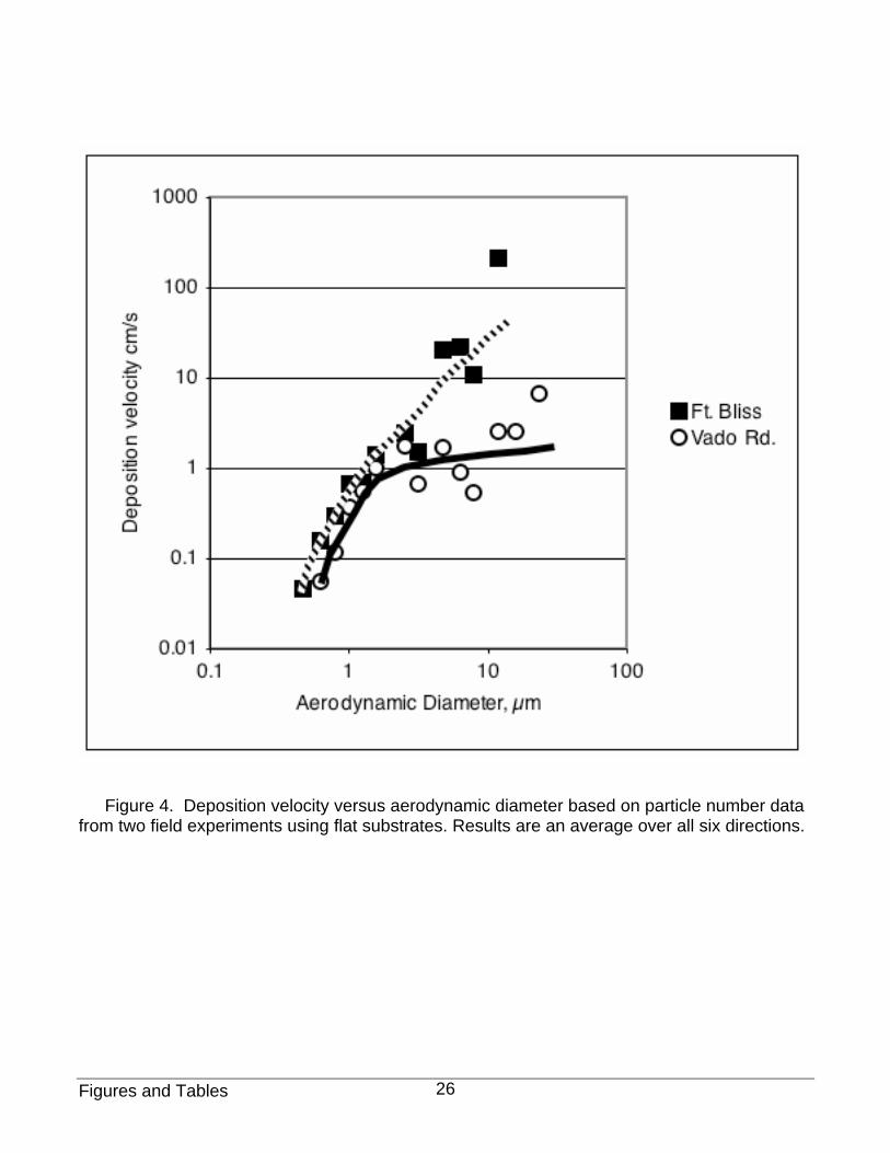
Figure 4. Deposition velocity versus aerodynamic diameter based on particle number data from two field experiments using flat substrates. Results are an average over all six directions.
Figures and Tables 26
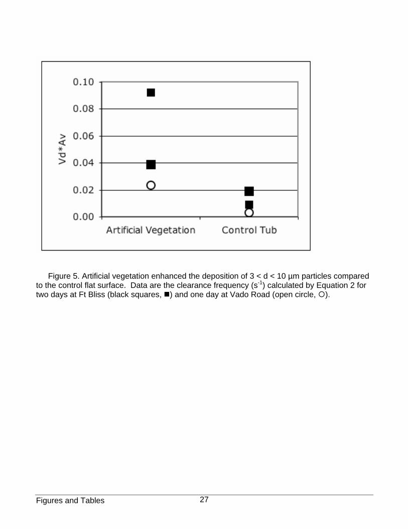
Figure 5. Artificial vegetation enhanced the deposition of 3 < d < 10 µm particles compared to the control flat surface. Data are the clearance frequency (s-1) calculated by Equation 2 for two days at Ft Bliss (black squares, ) and one day at Vado Road (open circle, ).
Figures and Tables 27
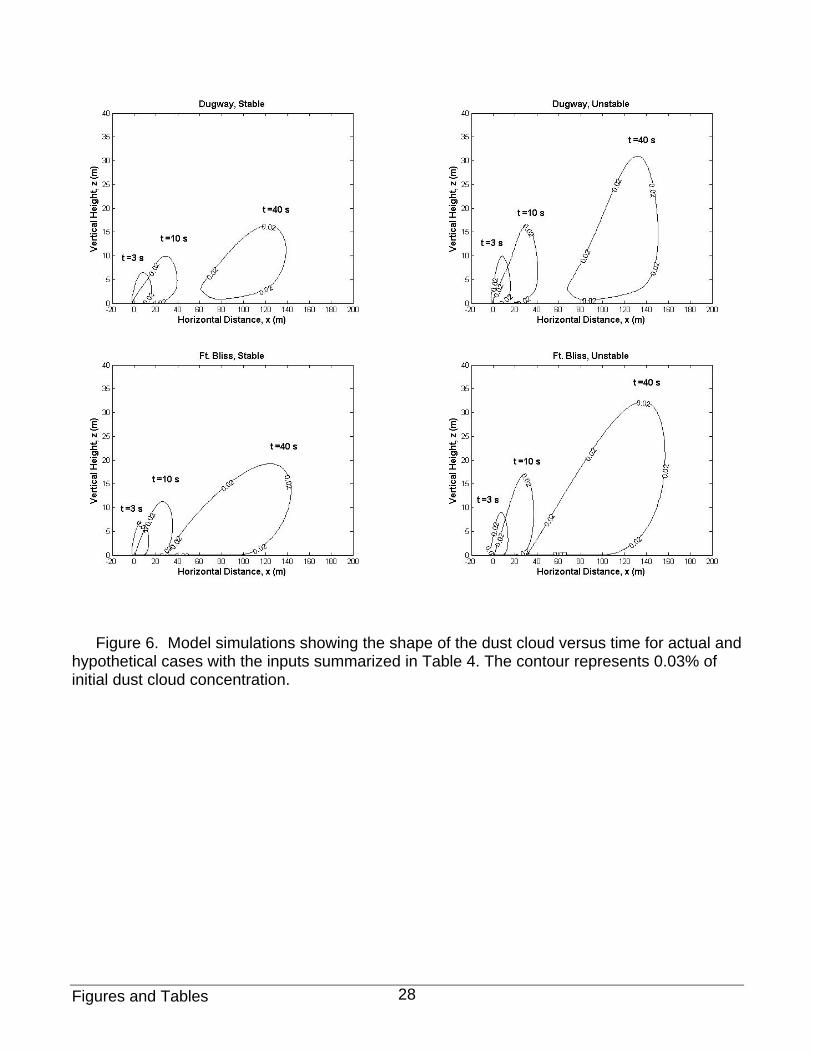
Figure 6. Model simulations showing the shape of the dust cloud versus time for actual and hypothetical cases with the inputs summarized in Table 4. The contour represents 0.03% of initial dust cloud concentration.
Figures and Tables 28
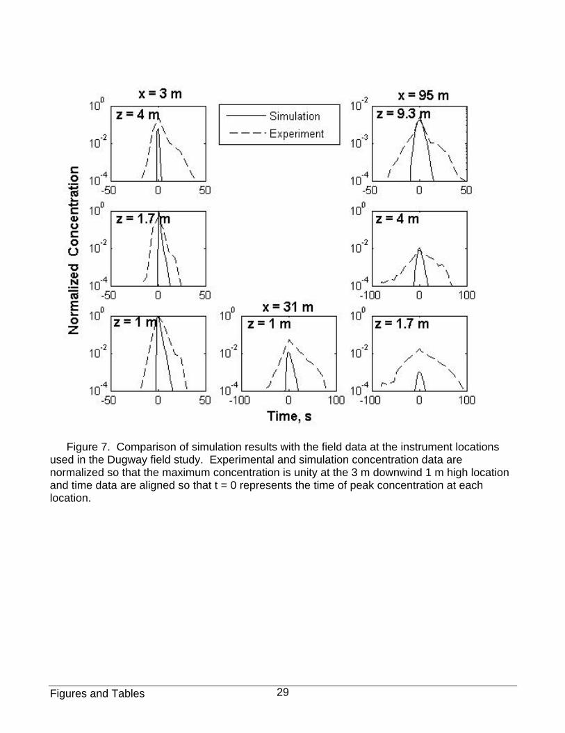
Figure 7. Comparison of simulation results with the field data at the instrument locations used in the Dugway field study. Experimental and simulation concentration data are normalized so that the maximum concentration is unity at the 3 m downwind 1 m high location and time data are aligned so that t = 0 represents the time of peak concentration at each location.
Figures and Tables 29
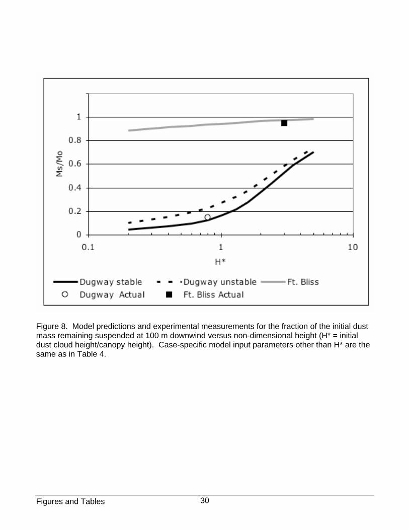
Figure 8. Model predictions and experimental measurements for the fraction of the initial dust mass remaining suspended at 100 m downwind versus non-dimensional height (H* = initial dust cloud height/canopy height). Case-specific model input parameters other than H* are the same as in Table 4.
Figures and Tables 30