ASSESSMENT OF WINDBREAKS AS A DUST CONTROL

STRATEGY FOR COMMUNITIES IN ARID CLIMATES SUCH

AS THE U.S.-MEXICAN BORDER REGION PROJECT NUMBER: A-04-03 ERIC R. PARDYJAK, UNIVERSITY OF UTAH SCOTT SPECKART, UNIVERSITY OF UTAH

NARRATIVE SUMMARY Dust generated from the mechanical disturbance of granular material is known as “fugitive dust” since it is not released into the atmosphere in a restricted flow stream such as an exhaust pipe or smoke stack. Fugitive dust includes dust from unpaved roads, disturbed land in developed areas, agriculture, and undeveloped grazing land. Wind-blown and vehicle generated fugitive dust are air quality and health concerns in many areas along the U.S.-Mexican border. Fugitive dust contains particulate mater (PM) smaller than 10µm (PM10). PM10 has been linked with numerous health problems. Air quality officials in the southwest are dissatisfied with the available options for controlling vehicle generated fugitive dust since water-based treatments are often impractical in arid climates. Previous SCERP-funded studies in Doña Ana County, New Mexico have examined the hypothesis that dust traveling near the ground is redeposited when it encounters brush, fences, and small terrain irregularities. A conclusion from this previous work was that atmospheric stability, time of day, surface roughness and nearby vegetation are important factors affecting the amount of vehicle-suspended dust that is actually transported a sufficient distance to affect local and regional air quality. Other field studies have supported this conclusion. The objective of the current project was to build on previous SCERP and related research to better understand dispersion of fugitive dust in the presence of vegetation when atmospheric conditions transition from unstable to stable conditions in the border desert environment. The second objective of this project has been to develop a computer model of the transport of vehicle generated fugitive dust. The modeling tool that has been developed is capable of reproducing important aspects of the field experiment from this project and other work. The model is particularly useful to planners and decision makers as it can provide estimates of the benefits that vegetation can provide for reducing fugitive dust under various atmospheric conditions.

2

ASSESSMENT OF WINDBREAKS AS A DUST CONTROL

STRATEGY FOR COMMUNITIES IN ARID CLIMATES SUCH

AS THE U.S.-MEXICAN BORDER REGION PROJECT NUMBER: A-04-03 ERIC R. PARDYJAK, UNIVERSITY OF UTAH SCOTT SPECKART, UNIVERSITY OF UTAH

INTRODUCTION Dust generated from the mechanical disturbance of granular material is known as “fugitive dust” since it is not released into the atmosphere in a restricted flow stream. Fugitive dust includes dust from unpaved roads, disturbed land in developed areas, agriculture, and undeveloped grazing land. Wind-blown and vehicle generated fugitive dust is an air quality and health concern in many areas along the U.S.-Mexican border. Fugitive dust contains particulate mater (PM) smaller than 10µm (PM10). PM10 has been linked with numerous health problems. Illnesses can include lung and heart disease and asthma. Severity can vary from chronic heath nuisances to death (Samet et al. 1998). Air quality officials in the southwest are dissatisfied with the available options for controlling vehicle generated fugitive dust since water-based treatments are often impractical in arid climates. Previous SCERP-funded studies in Doña Ana County, New Mexico have examined the hypothesis that dust traveling near the ground is redeposited when it encounters brush, fences, and small terrain irregularities. A conclusion from this work is that atmospheric stability, time of day, surface roughness and nearby vegetation are important factors affecting the amount of vehicle-suspended dust that is actually transported a sufficient distance to affect local and regional air quality. Other field studies have supported this conclusion. In one study, significant near-source dust removal under stable atmospheric conditions with downwind obstructions was observed (Veranth et al. 2003). A similar study observed that little if any deposition occurs under unstable atmospheric conditions with little vegetation Etyemezian, et al. (2004).

RESEARCH OBJECTIVES The research documented in this report encompasses a field experiment performed in Doña Ana County, New Mexico during the month of March 2005, along with a computer simulation code that models dust traveling downwind of a dirt road. The first objective of the current project was to build on previous SCERP and related research to better understand dispersion of fugitive dust in the presence of vegetation when atmospheric conditions transition from unstable to stable conditions in the border desert environment. The second objective of this project has been to develop a computer model of the transport of vehicle generated fugitive dust. The tool that has been developed is capable of

3

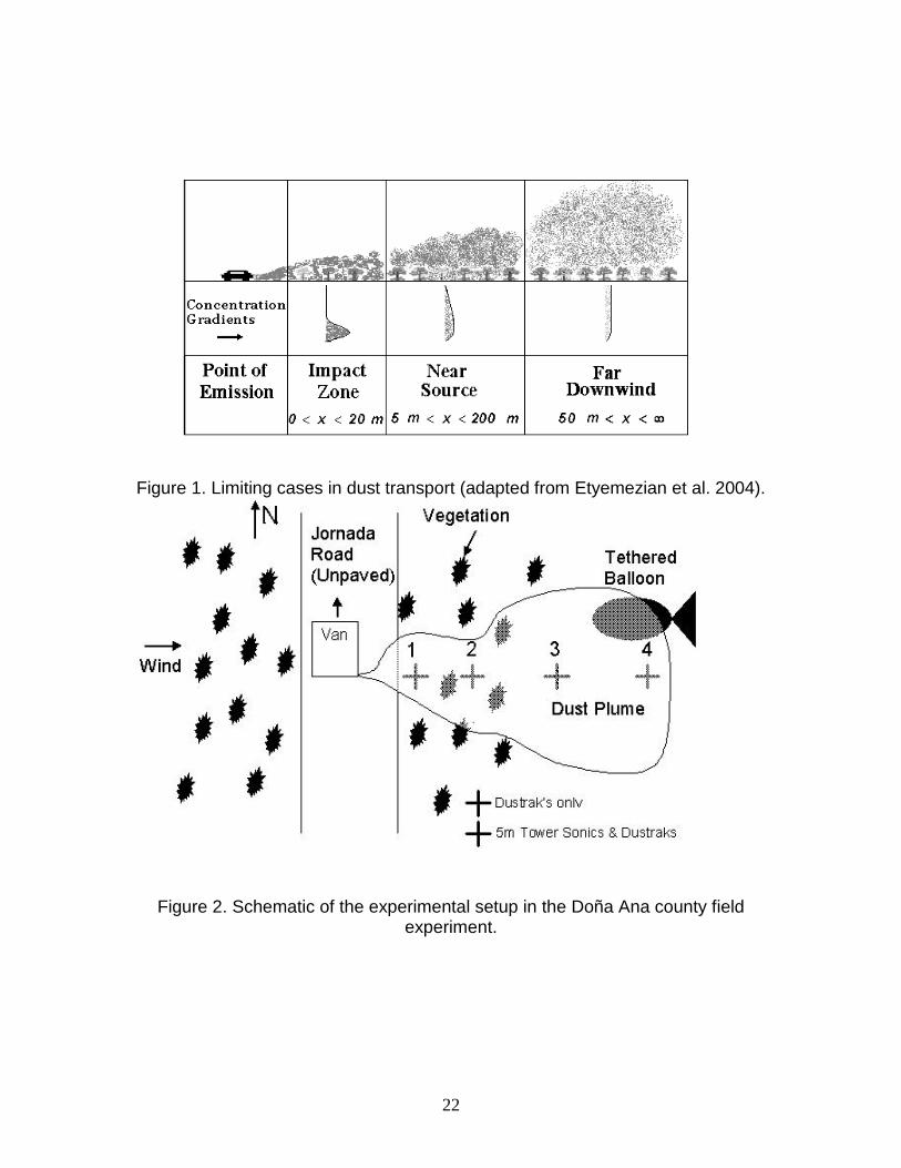
reproducing important aspects of the field experiment run as part this project and other work. The computer simulation has the ability to predict dust cloud behavior based upon atmospheric stability, surface roughness and nearby vegetation. Because of the inclusion of important characteristics, such as atmospheric stability and roughness, the computer modeling tool has helped to reconcile varying findings of previous fugitive dust studies. Additionally, the model is particularly useful to planners and decision makers as it can provide estimates of the benefits that vegetation can provide for reducing fugitive dust under various atmospheric conditions. RESEARCH METHODOLOGY/ APPROACHES Background Limiting cases for dust transport are shown in Figure 1 (adapted from Etyemezian et al. 2004). These include the impact, near source and far downwind zones. In the impact zone, the height of the dust cloud is of the same order of magnitude as the height of the vegetation. The concentration of dust is highest near the ground. In the near source case, the cloud is much taller and vertical concentration gradients are lower compared to the impact zone. In the far downwind zone, the dust is distributed throughout the atmospheric surface layer and concentration is not a function of height, except very near the ground. This study focuses on dust removal very close to the road where the dust cloud is in the impact zone. Etyemezian, et al. (2004) studied the behavior of a dust cloud downwind of a dirt road at Ft. Bliss, near El Paso, Texas during the period of April 11 to April 24, 2002. The resultant field data were compared to data from a Gaussian plume model in a near-road dust simulation.

The conditions of the experiment were of low surface roughness consisting of small dunes with widely spaced desert shrub vegetation, with roughness height, 0.001 m<zo<0.01 m, and neutral to unstable atmospheric conditions. The measurements indicated that the loss of PM10 within 100 m downwind of the source was less than 9.5%. The EPA ISC3 model, a Gaussian based model, indicated the loss of PM10 to be less than 5%. Etyemezian concluded that the EPA ISC3 model is a simplistic, but reasonable first approximation to the problem. The experimental results also indicated that the Gaussian model was limited by the fact that the plume concentration was not a function of the friction velocity, u*. Gaussian models are an excellent engineering approximation for a point release high above the ground, such as emission from a tall stack, but road dust is emitted into the Impact Zone from ground level. Near the ground however, there are large wind velocity and dust concentration gradients as well as inhomogeneity in the turbulence field that complicate the modeling of dispersion of dust.

Veranth, et al. (2003) studied a similar problem under different conditions. A field campaign lasting from September 6 to September 27, 2001 was run at the Dugway Proving Grounds in Utah to investigate the loss of PM10 downwind of an unpaved road under stable atmospheric conditions. The surface roughness was

4

high due to the placement of shipping containers in a rectangular 10 X 12 array. The containers were 2.5 m high, 2.4 m deep and 12.2 m long. The data revealed a removal of 85% for PM10 within the first 100 m downwind. Etyemezian also used the Gaussian based model to analyze this experiment and assumed very stable conditions and a much larger roughness height (zo=0.71 m,) than for the Ft. Bliss study. The Gaussian model predicted only 30% removal for the Dugway experiment.

Experiment Description The Doña Ana County study described in this report is for an arid region with little vegetation subject to transitional atmospheric conditions associated with the sunset. The site for this fugitive road dust study was La Jornada Road (N 32° 25.589’ W 106° 43.658’) located just northeast of Las Cruces, New Mexico from March 16 through March 18, 2005. The vegetation on the site was composed of Creosote and Mesquite with an average height of approximately 1.4 m. Grasses were also present on the site with heights in the range of 40-60 cm.

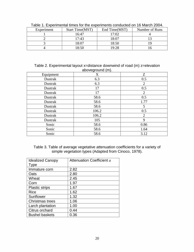
The most useful sets of experiments were on March 16, 2005 from the hours of 16:47 to 19:28. Due to the changing atmospheric stability during sunset, the experiment has been divided into four parts as described in Table 1. The sunset was at 18:11. As in the previous Dugway and Ft. Bliss studies (Veranth et al. 2003) the times of individual passes of an automobile were recorded.

The dust cloud associated with each automobile pass was manually identified (as described below) by inspecting each run and average PM10 concentrations were calculated using the following equation (equation 1):

ft

tiif

a dttctt

c )(1

(1)

ca is average dust concentration c(t) is instantaneous dust concentration tf Final time of pass of dust cloud ti Initial time of dust cloud

The concentrations were measured at four locations downstream of the unpaved road (and at multiple locations in the vertical direction) using TSI, Inc. Dustraks with PM10 inlets sampling at a rate of 1Hz. Vertical profiles of three dimensional velocity measurements were acquired using a set of 3 Campbell Scientific CSAT3 sonic anemometers mounted at heights of 0.86, 1.64 and 3.12 m. The

5

data from the anemometers were recorded at 10Hz and saved to a Campbell Scientific CR5000 data logger. The equipment used is shown schematically in Figure 2 and listed in Table 2 along with location in the experiment.

For this experiment, a continuous dust plume was approximated by ensemble averaging a number of individual dust clouds created by a single vehicle driving by. The dust cloud associated with each automobile pass was manually identified by inspecting each run and average PM10 concentration. The plume was assumed to pass by the sensor when the concentrations levels exceeded the background concentrations that were assumed to be ~ 0.001 mg/m3. A concentration pulse was defined as the period of time during which the measurements exceeded the ambient concentration threshold for at least four seconds. The end of a pulse was defined when the ambient threshold was met for four seconds. If there were multiple pulses in the same run, these multiple pulses were attributed to the same run. For the 10 Dustraks over the 50 runs multiple pulses occurred about 40 times (i.e., <10% of the time).

The horizontal flux of PM10 past the towers at the side of the road at x=6.3 m and x=106 m were calculated and compared to determine percent deposition. The elevations of the Dustraks are noted in table 2.

To calculate that net horizontal flux of PM10 the following equation was implemented:

T

dzdttzutzcFlux0 0

),(*),(

c(z,t) The dust concentration profile as a function of height above ground u(z,t) The mean horizontal wind as a function of height above ground t Time for dust cloud to pass a set point

To determine the flux of PM10, two profiles obtained from interpolations are necessary. First the interpolation of wind speed was accomplished by using a logarithmic curve of the form

oz

zuzu ln)( *

Κ Von Karman constant

*u friction velocity (m/s)

zo aerodynamic roughness length (m)

stability function =4.7(z/L)

6

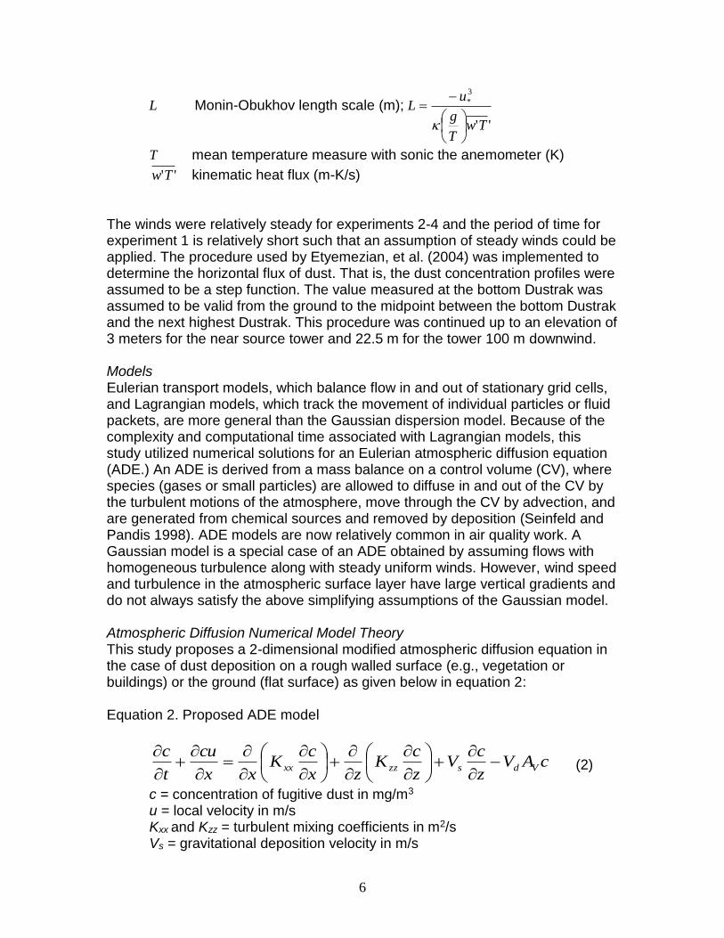
L Monin-Obukhov length scale (m);

''

3

*

TwT

g

uL

T mean temperature measure with sonic the anemometer (K)

''Tw kinematic heat flux (m-K/s)

The winds were relatively steady for experiments 2-4 and the period of time for experiment 1 is relatively short such that an assumption of steady winds could be applied. The procedure used by Etyemezian, et al. (2004) was implemented to determine the horizontal flux of dust. That is, the dust concentration profiles were assumed to be a step function. The value measured at the bottom Dustrak was assumed to be valid from the ground to the midpoint between the bottom Dustrak and the next highest Dustrak. This procedure was continued up to an elevation of 3 meters for the near source tower and 22.5 m for the tower 100 m downwind.

Models Eulerian transport models, which balance flow in and out of stationary grid cells, and Lagrangian models, which track the movement of individual particles or fluid packets, are more general than the Gaussian dispersion model. Because of the complexity and computational time associated with Lagrangian models, this study utilized numerical solutions for an Eulerian atmospheric diffusion equation (ADE.) An ADE is derived from a mass balance on a control volume (CV), where species (gases or small particles) are allowed to diffuse in and out of the CV by the turbulent motions of the atmosphere, move through the CV by advection, and are generated from chemical sources and removed by deposition (Seinfeld and Pandis 1998). ADE models are now relatively common in air quality work. A Gaussian model is a special case of an ADE obtained by assuming flows with homogeneous turbulence along with steady uniform winds. However, wind speed and turbulence in the atmospheric surface layer have large vertical gradients and do not always satisfy the above simplifying assumptions of the Gaussian model.

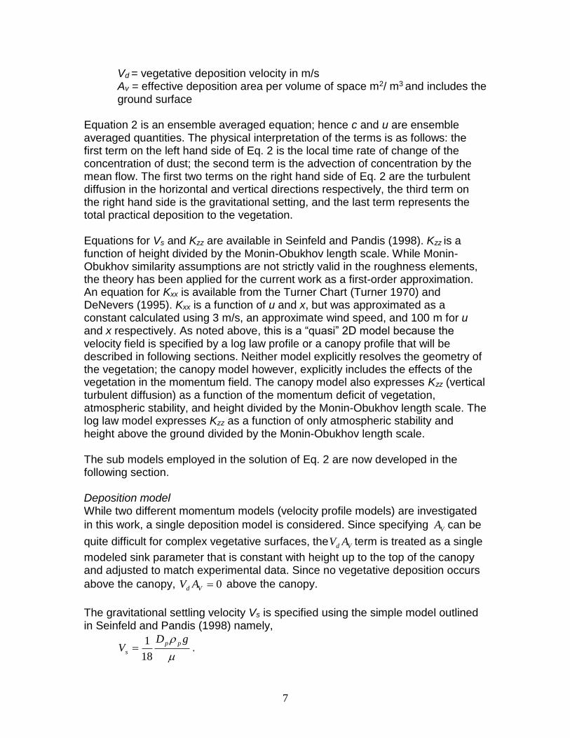
Atmospheric Diffusion Numerical Model Theory This study proposes a 2-dimensional modified atmospheric diffusion equation in the case of dust deposition on a rough walled surface (e.g., vegetation or buildings) or the ground (flat surface) as given below in equation 2: Equation 2. Proposed ADE model

cAVz

cV

z

cK

zx

cK

xx

cu

t

cVdszzxx

(2)

c = concentration of fugitive dust in mg/m3

u = local velocity in m/s Kxx and Kzz = turbulent mixing coefficients in m2/s Vs = gravitational deposition velocity in m/s

7

Vd = vegetative deposition velocity in m/s Av = effective deposition area per volume of space m2/ m3 and includes the ground surface

Equation 2 is an ensemble averaged equation; hence c and u are ensemble averaged quantities. The physical interpretation of the terms is as follows: the first term on the left hand side of Eq. 2 is the local time rate of change of the concentration of dust; the second term is the advection of concentration by the mean flow. The first two terms on the right hand side of Eq. 2 are the turbulent diffusion in the horizontal and vertical directions respectively, the third term on the right hand side is the gravitational setting, and the last term represents the total practical deposition to the vegetation.

Equations for Vs and Kzz are available in Seinfeld and Pandis (1998). Kzz is a function of height divided by the Monin-Obukhov length scale. While Monin-Obukhov similarity assumptions are not strictly valid in the roughness elements, the theory has been applied for the current work as a first-order approximation. An equation for Kxx is available from the Turner Chart (Turner 1970) and DeNevers (1995). Kxx is a function of u and x, but was approximated as a constant calculated using 3 m/s, an approximate wind speed, and 100 m for u and x respectively. As noted above, this is a “quasi” 2D model because the velocity field is specified by a log law profile or a canopy profile that will be described in following sections. Neither model explicitly resolves the geometry of the vegetation; the canopy model however, explicitly includes the effects of the vegetation in the momentum field. The canopy model also expresses Kzz (vertical turbulent diffusion) as a function of the momentum deficit of vegetation, atmospheric stability, and height divided by the Monin-Obukhov length scale. The log law model expresses Kzz as a function of only atmospheric stability and height above the ground divided by the Monin-Obukhov length scale.

The sub models employed in the solution of Eq. 2 are now developed in the following section.

Deposition model While two different momentum models (velocity profile models) are investigated

in this work, a single deposition model is considered. Since specifying VA can be

quite difficult for complex vegetative surfaces, the Vd AV term is treated as a single

modeled sink parameter that is constant with height up to the top of the canopy and adjusted to match experimental data. Since no vegetative deposition occurs

above the canopy, 0Vd AV above the canopy.

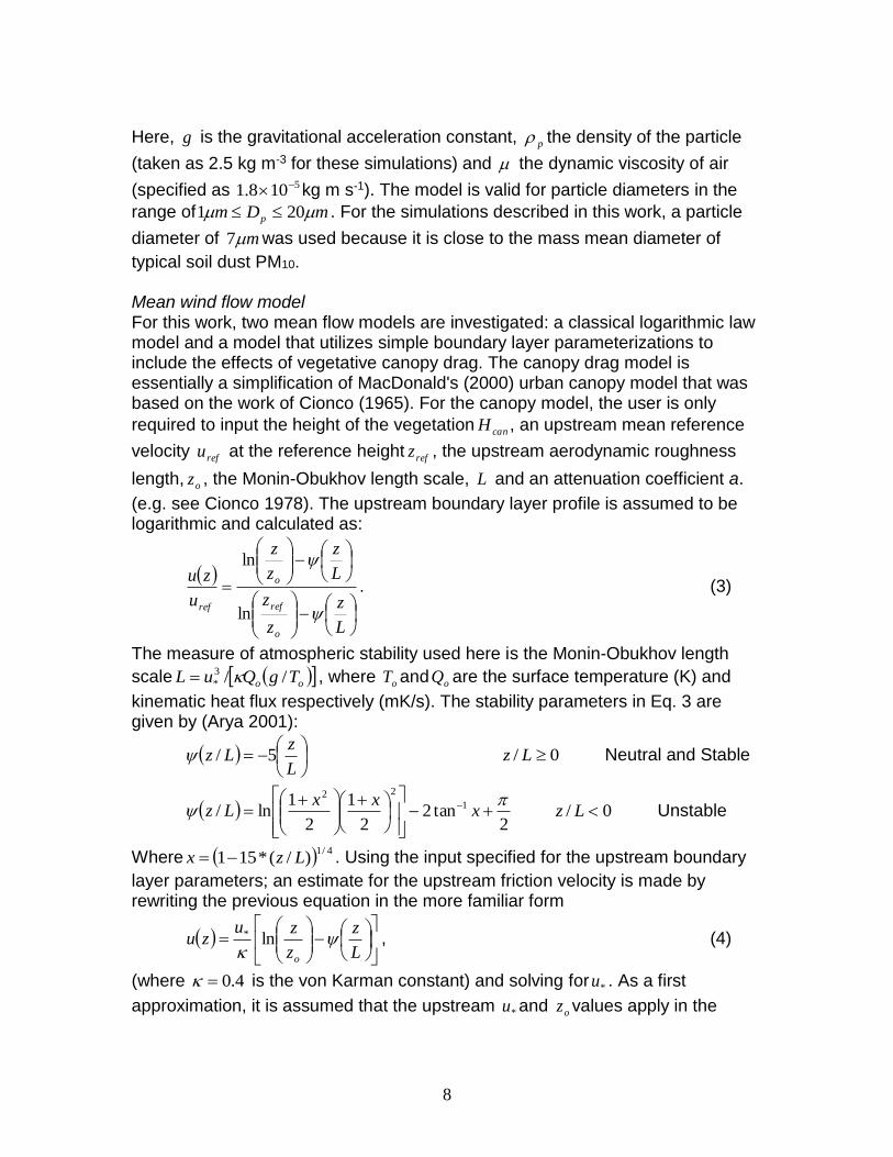
The gravitational settling velocity Vs is specified using the simple model outlined in Seinfeld and Pandis (1998) namely,

gDV

pp

s18

1 .

8

Here, g is the gravitational acceleration constant, p the density of the particle

(taken as 2.5 kg m-3 for these simulations) and the dynamic viscosity of air

(specified as 5108.1 kg m s-1). The model is valid for particle diameters in the

range of mDm p 201 . For the simulations described in this work, a particle

diameter of m7 was used because it is close to the mass mean diameter of

typical soil dust PM10. Mean wind flow model For this work, two mean flow models are investigated: a classical logarithmic law model and a model that utilizes simple boundary layer parameterizations to include the effects of vegetative canopy drag. The canopy drag model is essentially a simplification of MacDonald's (2000) urban canopy model that was based on the work of Cionco (1965). For the canopy model, the user is only

required to input the height of the vegetation canH , an upstream mean reference

velocity refu at the reference height refz , the upstream aerodynamic roughness

length, oz , the Monin-Obukhov length scale, L and an attenuation coefficient a.

(e.g. see Cionco 1978). The upstream boundary layer profile is assumed to be logarithmic and calculated as:

L

z

z

z

L

z

z

z

u

zu

o

ref

o

ref

ln

ln

. (3)

The measure of atmospheric stability used here is the Monin-Obukhov length

scale oo TgQuL //3

* , where oT and oQ are the surface temperature (K) and

kinematic heat flux respectively (mK/s). The stability parameters in Eq. 3 are given by (Arya 2001):

L

zLz 5/ 0/ Lz Neutral and Stable

2

tan22

1

2

1ln/ 1

22

x

xxLz 0/ Lz Unstable

Where 4/1)/(*151 Lzx . Using the input specified for the upstream boundary

layer parameters; an estimate for the upstream friction velocity is made by rewriting the previous equation in the more familiar form

L

z

z

zuzu

o

ln* , (4)

(where 4.0 is the von Karman constant) and solving for *u . As a first

approximation, it is assumed that the upstream *u and oz values apply in the

9

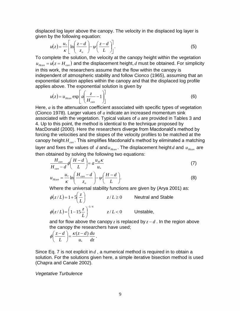
displaced log layer above the canopy. The velocity in the displaced log layer is given by the following equation:

L

dz

z

dzuzu

o

ln* . (5)

To complete the solution, the velocity at the canopy height within the vegetation

canHcan Hzuu and the displacement height, d must be obtained. For simplicity

in this work, the researchers assume that the flow within the canopy is independent of atmospheric stability and follow Cionco (1965), assuming that an exponential solution applies within the canopy and that the displaced log profile applies above. The exponential solution is given by

1exp

can

HcanH

zauzu (6)

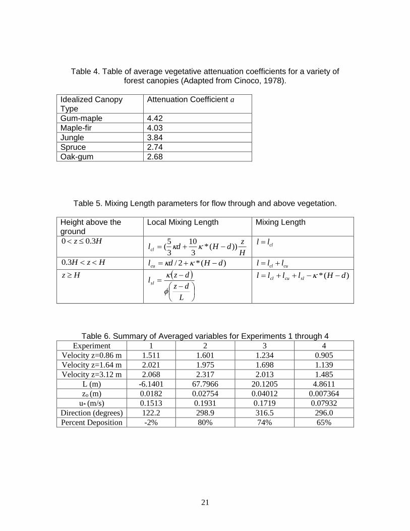
Here, a is the attenuation coefficient associated with specific types of vegetation (Cionco 1978). Larger values of a indicate an increased momentum sink associated with the vegetation. Typical values of a are provided in Tables 3 and 4. Up to this point, the method is identical to the technique proposed by MacDonald (2000). Here the researchers diverge from Macdonald’s method by forcing the velocities and the slopes of the velocity profiles to be matched at the

canopy height canH . This simplifies Macdonald’s method by eliminated a matching

layer and fixes the values of d and Hcanu . The displacement height d and Hcanu are

then obtained by solving the following two equations:

*u

ua

L

dH

dH

H H

can

can

(7)

L

dH

z

dHuu

o

can

Hcan

ln* . (8)

Where the universal stability functions are given by (Arya 2001) as:

L

zLz 51/ 0/ Lz Neutral and Stable

4/1

151/

L

zLz 0/ Lz Unstable,

and for flow above the canopy z is replaced by dz . In the region above

the canopy the researchers have used;

dz

du

u

dz

L

dz

*

)(

.

Since Eq. 7 is not explicit in d , a numerical method is required in to obtain a

solution. For the solutions given here, a simple iterative bisection method is used (Chapra and Canale 2002). Vegetative Turbulence

10

The vertical turbulent flux of particle concentration within the vegetation is modeled using a simple gradient method

z

cKcw zz

''

as shown in Eq. 2 above. In this model, the assumption is made that diffusion

coefficient zzK is the same as the momentum diffusion coefficient. Hence, in the

simple log law boundary layer model, zzK is specified based on Monin-Obukhov

similarity as

Lz

zuK zz

/

*

.

In the modified canopy model, this same expression is used upwind of the canopy and above the canopy, however z is replaced by dz for above the

canopy. Within the canopy, a mixing length model that is independent of atmospheric stability is assumed and specified in the form:

z

uK

z

ulwu zz

2

2'' .

Using the mixing length ideas for flow in vegetation given by Cionco (1965) yields the following expression for the diffusion coefficient:

z

ulK zz

2 .

The velocity gradient is calculated directly using finite differences from the mean flow field described above. The mixing length scale is modeled as the sum of the canopy length scale and the surface layer length scale, namely,

slc lll .

Above the canopy, a simple mixing length model is assumed, where the mixing length is given by:

L

dz

dzklsl

.

Within the canyon, the mixing length is assumed to increase linearly from the ground to z= 0.3H, following Cionco (1965). Above z= 0.3H the mixing length is taken to be a constant value given in Table 5.

The canopy mixing length cuclc lll is derived as follows (similar to Poggi et al.

[2004]): it is based on two physical principles, one that high above the canopy as z the values for Kzz for the canopy and for the log models should approach

the same value. The second is that the mixing length should be a continuous function. This is enforced at the canopy top as explained later.

11

Returning to the first principle for neutral conditions as z , the following

equation is suggested:

))(/()( *

2

* dzkulllzku slcucl .

Note that 1 Ldz for neutral conditions. When this equation is expanded

and solved for cucl ll a quadratic in cucl ll results. Solving this quadratic, using

the definition for sll for neutral conditions, and using the positive, physically

plausible root gives:

)(*))/(11( dzkdzdll cucl .

In the limit as z , the right hand side is of the indeterminate type 0 * ∞.

Applying L’Hôpital’s rule once gives a value of 2/kdll cucl . Because the

conditions in the vegetative canopy are assumed to be neutral always this value is independent of atmospheric stability. To satisfy the second condition of continuity of the mixing length, a second term

is included in cucl ll . The reason for the need of a second term is a discontinuity

present at the canopy top at Hz when 2/kdll cucl . Above the canopy the

value is )(*2 dHkkd , thus there is a discontinuous jump in the mixing length

at Hz . The magnitude of this discontinuity is )(* dHk . Thus )(* dHk is

added to the value of cucl ll . This second term is only applied in the canopy.

It should be noted that although the conditions in the canopy are assumed independent of stability a dependence of stability is introduced by using the value of d obtained by matching the exponential and logarithmic curves as documented

earlier in this work. The dependence of cucl ll upon atmospheric stability will be

documented in a later work. . Numerical Implementation The velocity profiles and turbulence models described above are input into a numerical simulation of equation 1 written in Matlab. The Spatial domain is rectangular with a length of 630m and a height of 50m. The lengthwise distance is perpendicular to the direction of the road and along the predominant wind direction. The road is located as to have 30m of the computational domain located upwind of the road and 600m downwind of the road.

This spatial domain is characterized using finite volumes (Versteeg and Malalasekera 1995). The advective terms are modeled by a first order upwind finite difference. The diffusive terms are modeled by second order central differences. The body terms are exact.

Temporal dependence of equation 1 is modeled by using an Alternating Direction Implicit technique (Anderson 1995). Variable time steps are used during the 125s

12

simulation time. Smaller time steps of the order of 0.01s are used in the first 10s. Larger time steps of the order of 0.25 to 1s are used for the rest of the simulation.

To minimize computational effort, a non-uniform mesh is utilized (Anderson 1995). To achieve this, equation 2 is solved on a logarithmic mesh. Equation 2 is modified. This modification involves using the chain rule from Calculus to express the derivatives in term of new uniform variables and solving this modified equation in the new uniform computational space. The results are then interpreted in terms of the non uniform physical space.

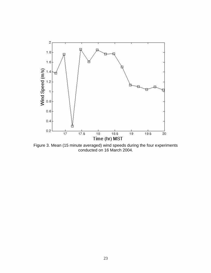
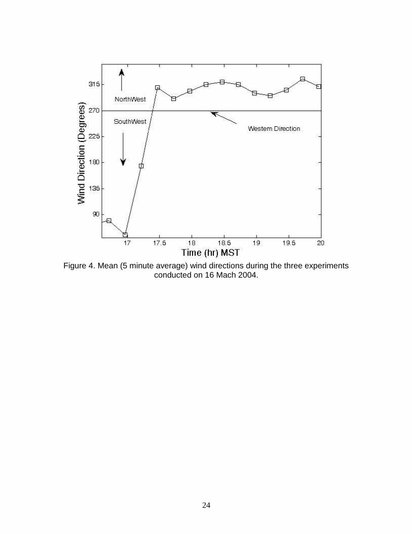
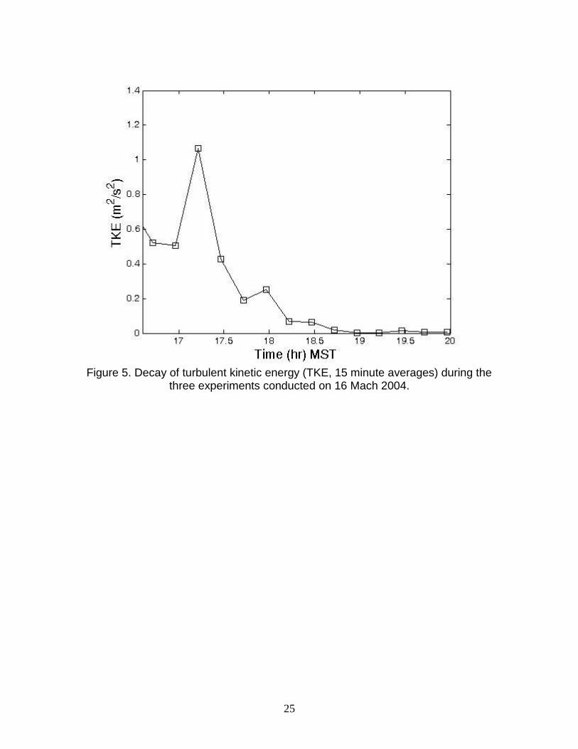
A typical simulation runs on a Celeron PC laptop in about two and a half minutes. This involves about 30,000 nodes and 500 time steps. The large number of time steps is because to insure mass conservation, the simulation is performed twice, one without vegetative deposition and another with vegetative deposition. RESEARCH FINDINGS Experiment Results The atmospheric conditions of the Doña Ana county experiment are shown in Figures 3 through 8 and displayed in Table 6. Table 6 contains seven variables averaged for each of the four experiments. The first three variables are mean wind velocity at different elevations above the ground. The fourth variable is the Monin-Obukhov length scale, L. The roughness height, zo, the friction velocity, (ustar u*) and wind direction. The table illustrates, that as expected, wind speed increases with elevation in a near logarithmic manner as shown in the table. The data show a clear smooth transition from unstable conditions to stable conditions with a flip in surface heat flux sign occurring at about 17:45 local time. Accordingly, the Monin-Obukhov length scale is negative for experiment one and hence indicative of an unstable atmospheric for experiment one. As time passes, the Monin-Obukhov length scale changes to positive values, indicative of stable atmospheric conditions. The mean wind direction also changes from a northeastern direction to a northwestern direction in between experiments 1 and 2. The mean wind speed, measured at z=1.64 m, is shown in Figure 3. The wind velocity has a distinct minimum between the time of 17:00 and 17:30. Further insight may be gained by observing Figure 4, where low mean wind speeds correspond to a major change in wind direction. It may be noted that the winds are from the northeastern direction at the start of the four experiments and change to a northwestern direction for the remaining period of experiments. Sunset on March 16, 2005 was 18:11, so this transformation in wind speed and direction is related to the transition from a daytime convective boundary layer to a stable nocturnal layer. In Figure 5, the decay of turbulent kinetic energy is plotted. The late afternoon hours have large values for turbulent kinetic energy (TKE) indicative of unstable

13

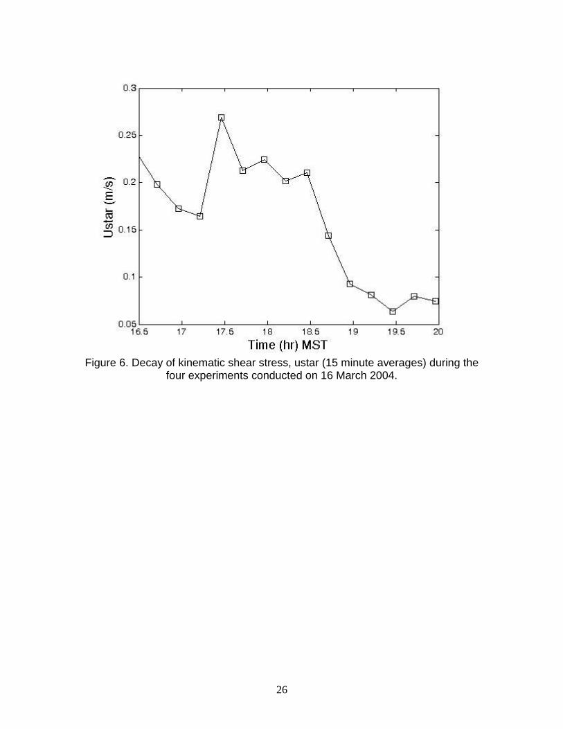
atmospheric conditions. As time progresses, and the evening hours start the amount of TKE decays to those more indicative of stable atmospheric conditions. Figure 6 also chronicles the transition from an unstable atmospheric condition to

a stable condition. The decay in the kinematic shear stress, *u (ustar) is plotted.

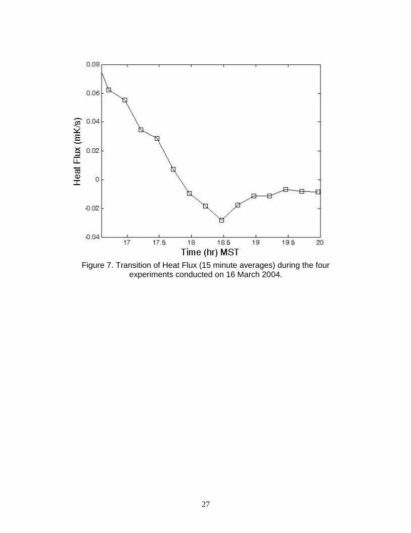
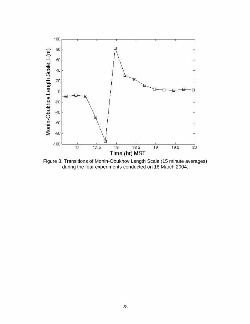
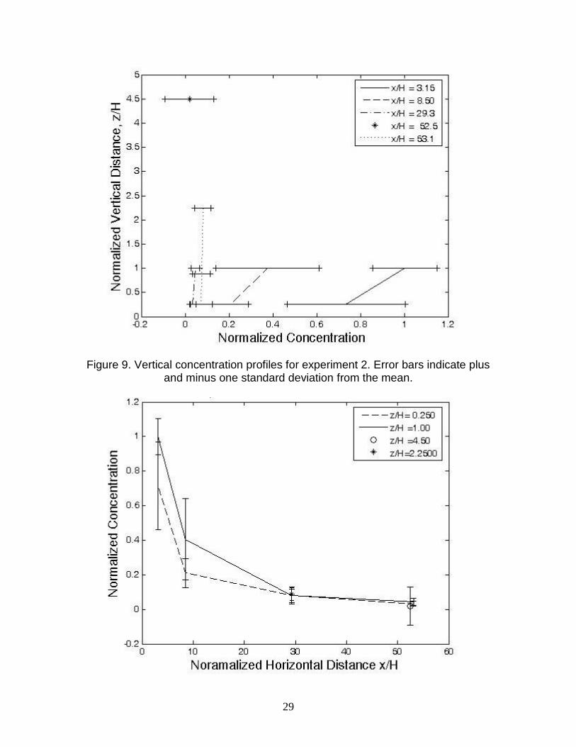
Early in the experiments, during the late afternoon hours, the unstable conditions generate high values of ustar associated with convective mixing. As the sun sets and initializes the transition to stable conditions the magnitude of the kinematic shear stress decreases. Figures 7 and 8 also display the transition from convective daytime heating to stable nocturnal conditions. Figure 7 displays the change from positive heat flux values, indicative of daytime heating to negative values indicative of the ground cooling. The heat flux is approximately zero between the hours of 17:30 and 18:00. It should again be noted that the sunset was at 18:11. Figure 8 shows the change from positive Monin-Obukhov Length Scales to negative length scales as expected during the evening transition. The data indicate neutral stability between the hours of 17:30 and 18. Figures 9 through 11 illustrate the dependence upon spatial variables and atmospheric stability. Figure 9 is a plot of normalized mean concentration data from experiment 2. The local concentration is normalized by the maximum concentration observed during the run. This maximum concentration was always located at the top roadside Dustrak. The standard deviations for experiment 2 are also displayed in this figure in the form of horizontal bars. As shown, the PM10

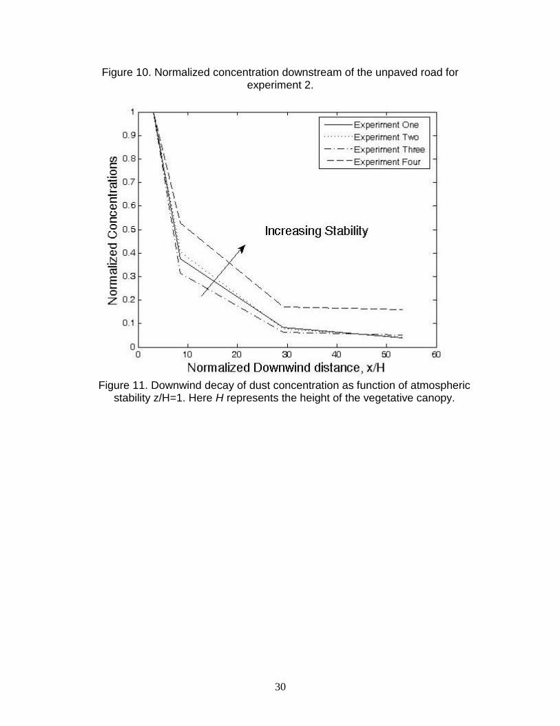
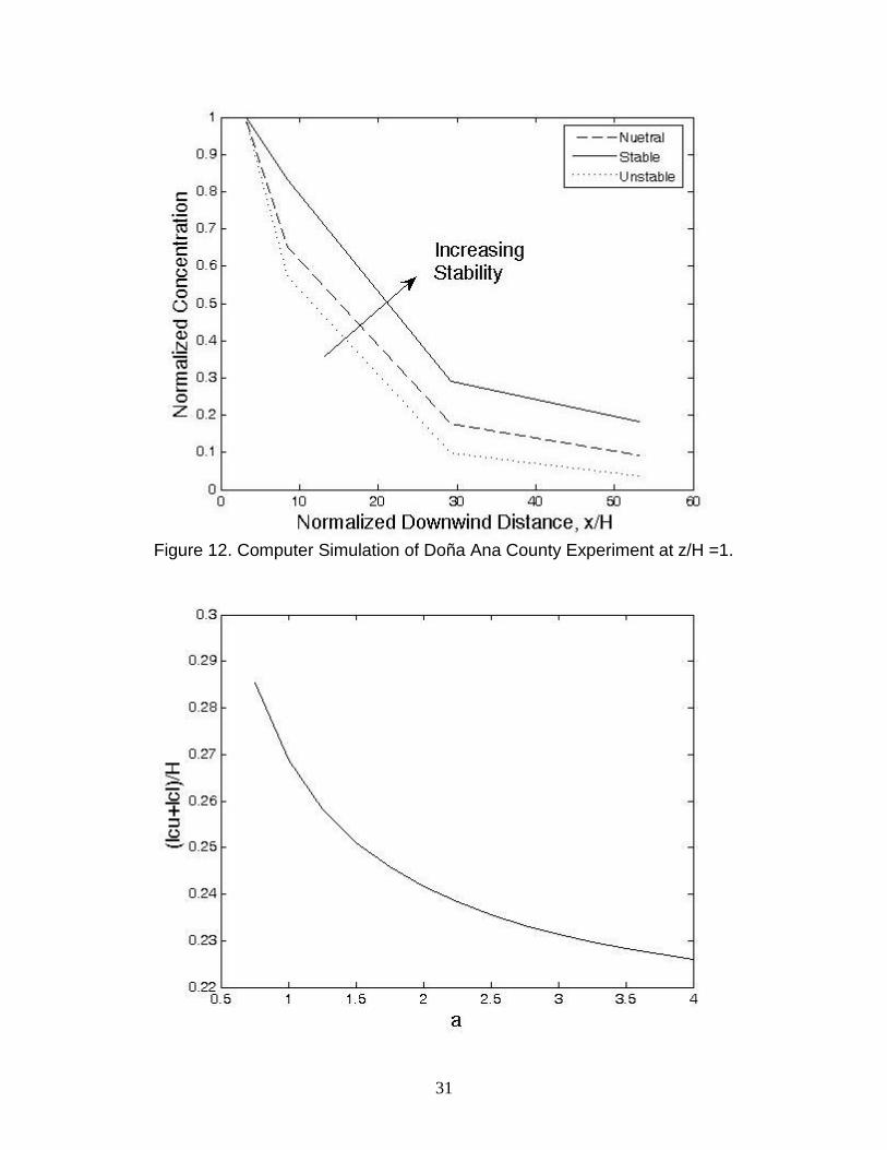
concentrations increase rapidly with height near the road and become more well-mixed further downstream. In Figure 10, the downwind decay of mean concentration is also displayed with standard deviations. As one may observe, the decay is exponential in form. The observation that concentrations become more uniform downwind is also displayed. The two lines converge to the same line with increasing distance downwind from the road. The two Dustraks that are located at higher elevations z/H= 2.25 and z/H=4.5 are also located at or near the convergence of these two lines. The downwind decay of mean dust concentration is displayed in Figure 11. The unique characteristic of Figure 11 is that it displays the change in this downward decay as a function of atmospheric stability. As one may observe, as atmospheric stability is increasing, the near ground concentration increases. This is because as atmospheric turbulence decays there is less dispersion of dust far from the ground, thus more dust remains near the ground. Figure 12 displays the result of a computer simulation of the Doña Ana County Experiment. It is identical in form to figure 11, a downwind display of dust concentration as a function of atmospheric stability. The computer simulation

14

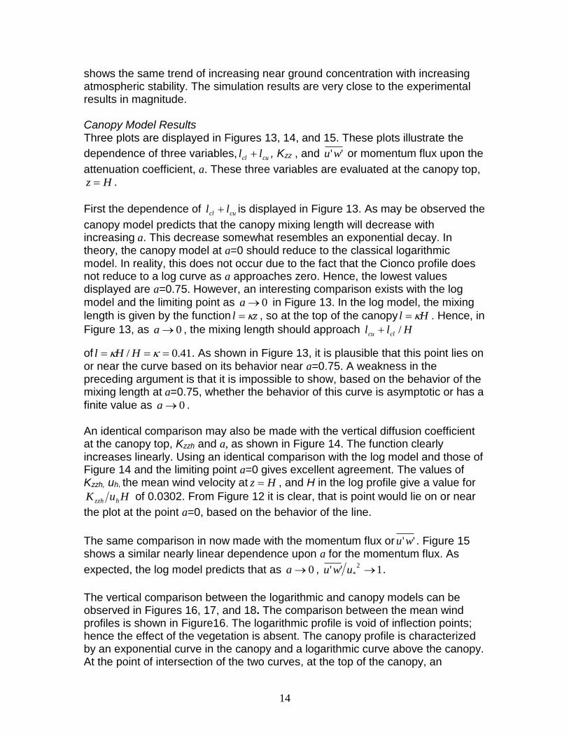
shows the same trend of increasing near ground concentration with increasing atmospheric stability. The simulation results are very close to the experimental results in magnitude. Canopy Model Results Three plots are displayed in Figures 13, 14, and 15. These plots illustrate the

dependence of three variables, cucl ll , Kzz , and ''wu or momentum flux upon the

attenuation coefficient, a. These three variables are evaluated at the canopy top, Hz .

First the dependence of cucl ll is displayed in Figure 13. As may be observed the

canopy model predicts that the canopy mixing length will decrease with increasing a. This decrease somewhat resembles an exponential decay. In theory, the canopy model at a=0 should reduce to the classical logarithmic model. In reality, this does not occur due to the fact that the Cionco profile does not reduce to a log curve as a approaches zero. Hence, the lowest values displayed are a=0.75. However, an interesting comparison exists with the log

model and the limiting point as 0a in Figure 13. In the log model, the mixing

length is given by the function zl , so at the top of the canopy Hl . Hence, in

Figure 13, as 0a , the mixing length should approach Hll clcu /

of 41.0/ HHl . As shown in Figure 13, it is plausible that this point lies on or near the curve based on its behavior near a=0.75. A weakness in the preceding argument is that it is impossible to show, based on the behavior of the mixing length at a=0.75, whether the behavior of this curve is asymptotic or has a

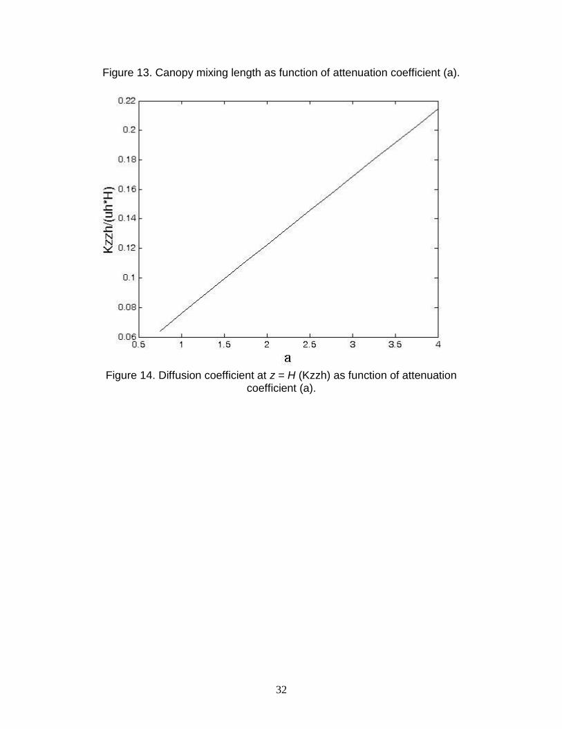
finite value as 0a . An identical comparison may also be made with the vertical diffusion coefficient at the canopy top, Kzzh and a, as shown in Figure 14. The function clearly increases linearly. Using an identical comparison with the log model and those of Figure 14 and the limiting point a=0 gives excellent agreement. The values of Kzzh, uh, the mean wind velocity at Hz , and H in the log profile give a value for

HuK hzzh of 0.0302. From Figure 12 it is clear, that is point would lie on or near

the plot at the point a=0, based on the behavior of the line.

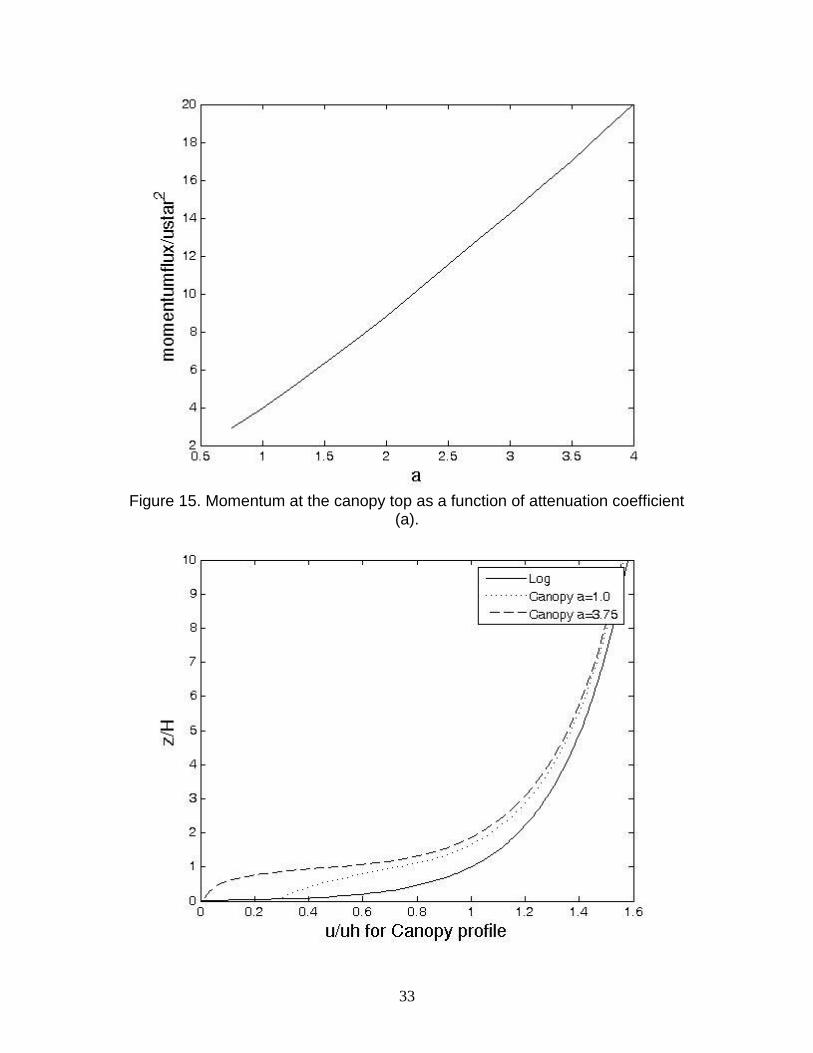
The same comparison in now made with the momentum flux or ''wu . Figure 15 shows a similar nearly linear dependence upon a for the momentum flux. As

expected, the log model predicts that as 0a , 1''2

* uwu .

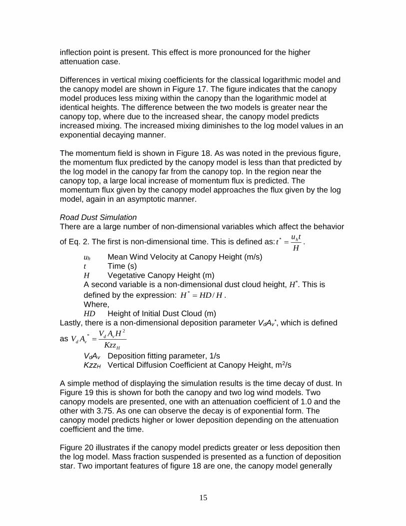
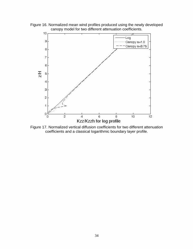
The vertical comparison between the logarithmic and canopy models can be observed in Figures 16, 17, and 18. The comparison between the mean wind profiles is shown in Figure16. The logarithmic profile is void of inflection points; hence the effect of the vegetation is absent. The canopy profile is characterized by an exponential curve in the canopy and a logarithmic curve above the canopy. At the point of intersection of the two curves, at the top of the canopy, an

15

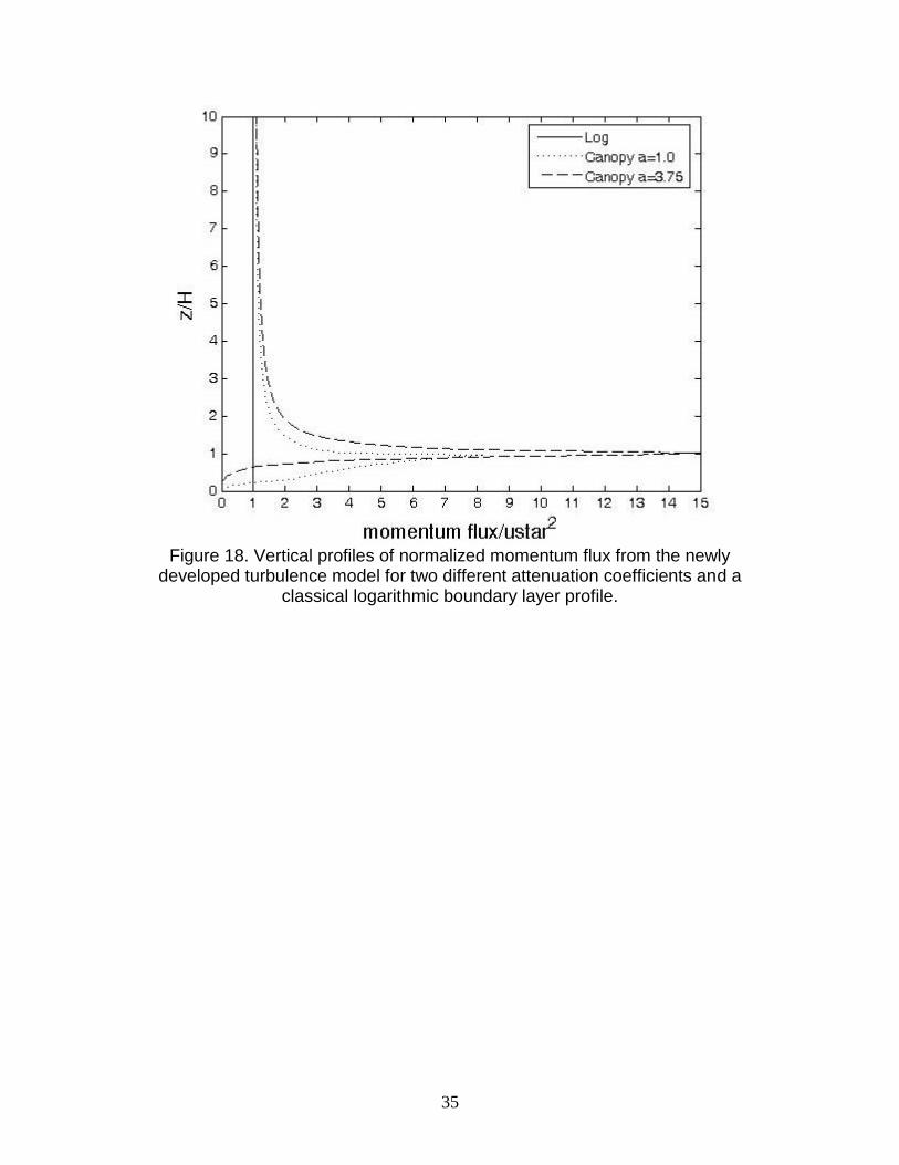
inflection point is present. This effect is more pronounced for the higher attenuation case. Differences in vertical mixing coefficients for the classical logarithmic model and the canopy model are shown in Figure 17. The figure indicates that the canopy model produces less mixing within the canopy than the logarithmic model at identical heights. The difference between the two models is greater near the canopy top, where due to the increased shear, the canopy model predicts increased mixing. The increased mixing diminishes to the log model values in an exponential decaying manner. The momentum field is shown in Figure 18. As was noted in the previous figure, the momentum flux predicted by the canopy model is less than that predicted by the log model in the canopy far from the canopy top. In the region near the canopy top, a large local increase of momentum flux is predicted. The momentum flux given by the canopy model approaches the flux given by the log model, again in an asymptotic manner. Road Dust Simulation There are a large number of non-dimensional variables which affect the behavior

of Eq. 2. The first is non-dimensional time. This is defined as:H

tut h* .

uh Mean Wind Velocity at Canopy Height (m/s) t Time (s) H Vegetative Canopy Height (m) A second variable is a non-dimensional dust cloud height, H*. This is

defined by the expression: HHDH /* . Where, HD Height of Initial Dust Cloud (m)

Lastly, there is a non-dimensional deposition parameter VdAv*, which is defined

as H

vd

vdKzz

HAVAV

2*

VdAv Deposition fitting parameter, 1/s KzzH Vertical Diffusion Coefficient at Canopy Height, m2/s

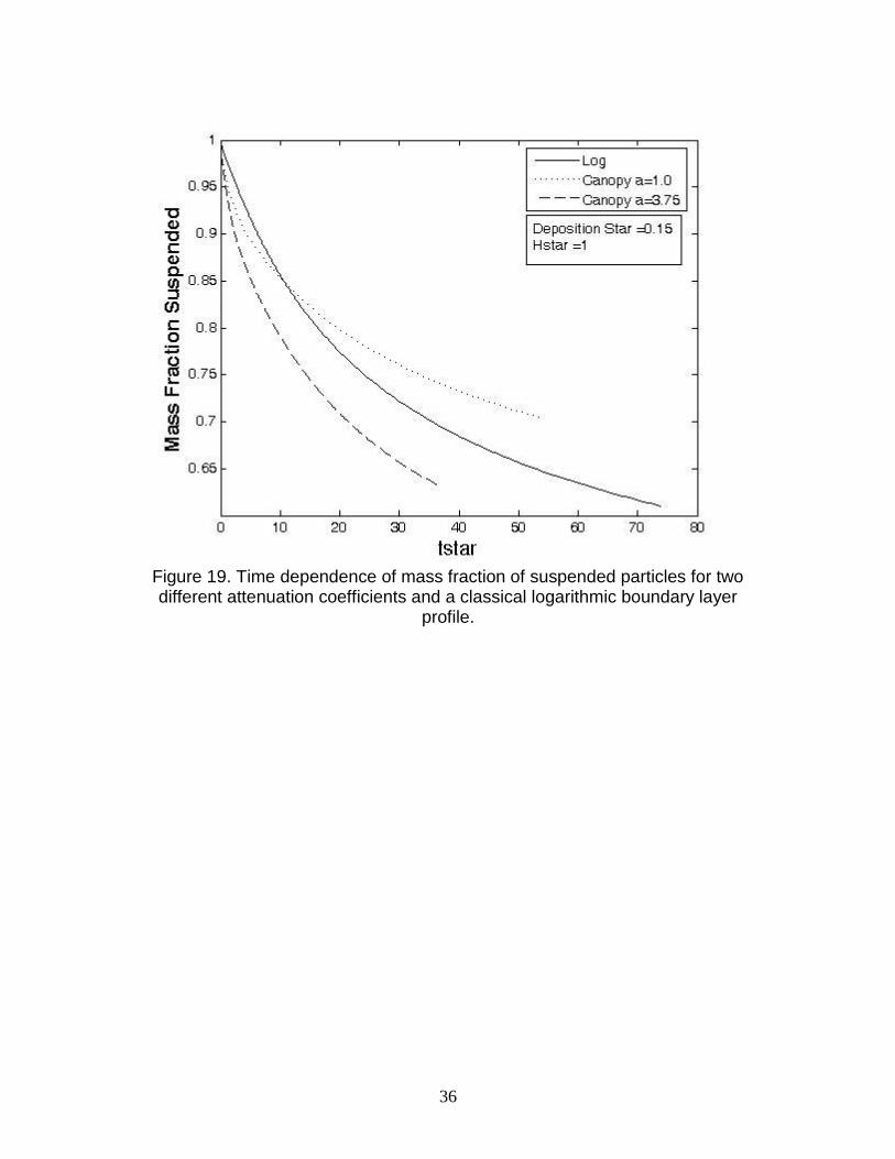
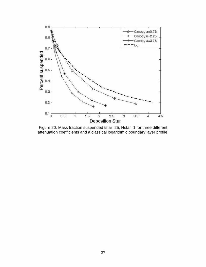
A simple method of displaying the simulation results is the time decay of dust. In Figure 19 this is shown for both the canopy and two log wind models. Two canopy models are presented, one with an attenuation coefficient of 1.0 and the other with 3.75. As one can observe the decay is of exponential form. The canopy model predicts higher or lower deposition depending on the attenuation coefficient and the time. Figure 20 illustrates if the canopy model predicts greater or less deposition then the log model. Mass fraction suspended is presented as a function of deposition star. Two important features of figure 18 are one, the canopy model generally

16

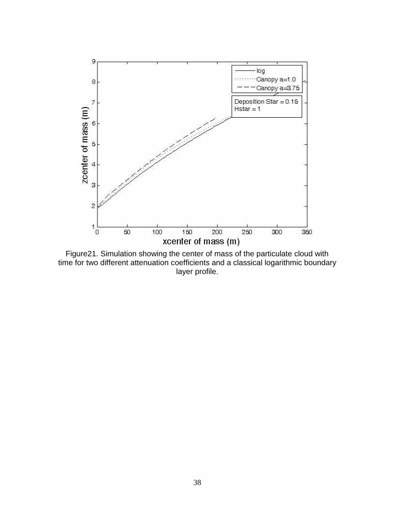
predicts more deposition, and the exception is at low deposition star values. The second feature is that all the canopy models converge at low depositions. The reason that the log model predicts greater deposition at low deposition star values is due to the interplay of two factors. The lower wind speed in the canopy model favors more deposition on the vegetation. However the additional shear present at the canopy top suspends dust higher in the canopy model than in the log model. This is shown in figure 21. This figure indicates that the higher the canopy attenuation coefficient, the higher the center of mass of the dust cloud. Because the dust is generally located higher in the canopy model this second factor tends to decrease the deposition predicted by the canopy model. At low deposition star values the second factor, the higher dust suspension dominates and the canopy models predict less deposition. At higher deposition star values the first factor the low wind speed factor dominates and the canopy models predict greater deposition.

CONCLUSIONS The aim of the present research was to develop a broader understanding of the near source transport and fate of vehicle generated fugitive dust in the arid U.S.-Mexican border region. Specifically, the researchers investigated vegetation as a dust mitigation strategy for enhancing near source deposition under varying atmospheric conditions. The specific outcomes of the work have been a unique experimental dataset from a field campaign in Las Cruces, NM and a computer model capable of predicting the transport of vehicle generated fugitive dust in the presence of vegetation.

The Las Cruces, Doña Ana county data provide additional insight into the behavior of a fugitive dust cloud in the near road region (within ~100 m) during the evening transition period. This is the time period before night when winds typically become very light and pollution levels can become quite high. To the researchers’ knowledge, this is the first vehicle generated fugitive dust study to provide PM and turbulence data during this period. The results indicate that as atmospheric stability increases, the concentration of PM10 increases. From these results, it appears that in general, if the vegetation is relatively sparse (as it was in this experiment), the PM10 concentrations will increase with increasing stability near the ground even though more deposition is expected onto the vegetation. In fact, the percent of suspended PM10 increased steadily with increasing stability. This is in contrast to the work of Veranth, et al. (2003), where periods of high stability resulted in enhanced deposition on large shipping containers with significant surface area. These results seem to indicate that a critical roughness associated with the vegetation may exist beyond which the stable boundary layer is destroyed and turbulence within the canopy is enhanced that encourages dispersion and deposition onto more available surface area. Along with the field study, the computer model has provided promising results in predicting dust cloud behavior based on atmospheric stability and the presence

17

of vegetation. The model is relatively easy to use and provides a tool for investigating different types of strategies for planting vegetation to mitigate fugitive dust that would be impossible to practically implement in the field. This work compared two different wind and turbulence models to simulate deposition onto vegetation: one that included the effects of a vegetative canopy and one that did not (the classical logarithmic model). It was found that for many rural border applications where vegetation is sparse that the simpler logarithmic produced reasonable results.

RECOMMENDATIONS FOR FURTHER RESEARCH Further research is needed to more fully comprehend the problem of dry deposition from fugitive road dust. Although many models currently exist, there are differences of order of magnitude in their predictions. Further comparative studies of the computer program results and experimental data would be greatly beneficial. Additionally, experiments that investigate the size ranges of particles that are most efficiently removed by different types of vegetation are necessary. Experiments that investigate a wide range of vegetative densities, heights (with respect to the dust cloud) and species along with manmade windbreaks are also necessary. The largest uncertainty in the model that has been proposed in this

report is the deposition term ( Vd AV ). The most efficient way to deal with this term

would be to run a series of simple wind tunnel experiments to develop useful empirical parameterizations over a broad range of vegetation types, particle sizes, etc. An additional simple research tax that would provide understanding regarding the economics of fugitive dust reduction would be a cost benefit analysis comparing different types of windbreak strategies to water based strategies. This would provide a sound basis for developing decision making strategies. RESEARCH BENEFITS This project benefits a diverse group of individuals, including air quality managers. To date, estimates of suspended near road fugitive dust over predict the amount of dust that is transported downwind a stuffiness distance to affect air quality. These experiments and modeling efforts help identify the extent of this issue for the border climate. Together with the previous fugitive dust studies, this study increases air quality and policy makers’ abilities to make informed decisions and formulate dust control strategies. By augmenting the understanding of the factors dominant in the transport of dust downwind of unpaved roads, the ability to perform more accurate predictions of dust transport becomes more plausible. The agreement between the Doña Ana county experiment and the model‘s predictions indicates that a simple atmospheric diffusion equation may be an improved option over many currently used models. This is of obvious benefit to those who live in areas

18

plagued with high fugitive dust concentrations, such as the U.S.-Mexican border region. It should be noted that the canopy model, which comprises part of the computer model, is also being adapted for Homeland Security applications of vegetative deposition funded by the DOE and DOD. ACKNOWLEDGMENTS The authors are indebted to J. Veranth for his contributions to theory development, experimental protocol and equipment use. The authors would like to thank Melessia Armijo and the office of public lands in the state of New Mexico for assistance in gaining proper paper work to perform the field experiment portion of this project. The authors would also like to thank FAA for the proper assistance in obtaining the proper permissions for flying the weather balloon. This work was sponsored by the Southwest Consortium for Environmental Research and Policy (SCERP) through a Cooperative agreement with the U.S. Environmental Protection Agency. SCERP can be contacted for further information through www.scerp.org and scerp@mail.sdsu.edu REFERENCES Anderson, J.D. (1995). Computational Fluid Dynamics, Mc GrawHill.

Arya, S. P., (2001). Introduction to Micrometeorology, 2nd Edition, Academic Press. Chapra, S.C. and Canale, R.P., (2002). Numerical Methods for Engineers, 4th edition. Mc GrawHill.

Cionco, R. M., (1965). Mathematical model for air flow in a vegetative canopy. J. Applied. Meteorol., 4, 517-522. Cionco, R. M., (1978). Analysis of canopy index values for various canopy densities. Boundary-Layer Meteorol. 15, 81-93.

De Nevers, N. (1995). Air pollution control engineering. New York, McGraw-Hill.

Etyemezian, V., S. Ahonen, D. Nikolic, J. Gilles, H. Kuhns, D. Gillette, and J. Veranth (2004). Deposition and Removal of Fugitive Dust in the Arid Southwestern United States: Measurements and Model Results. Journal of the Air and Waste Management Association 54: 1099 – 1111. MacDonald, R. W., (2000). Modeling the mean velocity profile in the urban canopy layer. Boundary-Layer Meteorology, 97, 25-45.

19

Poggi, D., Porporato, A., Ridolfi, L., Albertson, J.D., Katul, C.G. (2004). The Effect of Vegetation Density on Canopy Sub-Layer Turbulence. Boundary-Layer Meteorology, 111, 565-587

Samet, J.M., Zerer, S.L., et al. (1998). Particulate Air Pollution and Mortality: The Particle Epidemiology Evaluation Project. Applied Occupational and Environmental Health 13(6): 364-369.

Seinfeld, J.H. and Pandis, S.N. (1998). Atmospheric Chemistry and Physics — From Air Pollution to Climate Change. New York, Wiley.

Turner, D. B. (1970). Workbook of atmospheric dispersion estimates. Washington, U.S. Government Printing Office. Veranth, J. M., Seshadri, G. and Pardyjak, E. (2003). Vehicle-generated fugitive dust transport: Analytic models and field study. Atmospheric Environment 37(16): 2295-2303.

Versteeg and Malalasekera, (1995). An introduction to Computational Fluid Dynamics: The finite volume approach. Pearson Prentice Hall

20

Table 1. Experimental times for the experiments conducted on 16 March 2004. Experiment Start Time(MST) End Time(MST) Number of Runs

1 16:47 17:02 4

2 17:43 18:07 13

3 18:07 18:50 19

4 18:50 19:28 16

Table 2. Experimental layout x=distance downwind of road (m) z=elevation aboveground (m).

Equipment X Z

Dustrak 6.3 0.5

Dustrak 6.3 2

Dustrak 17 0.5

Dustrak 17 2

Dustrak 58.6 0.5

Dustrak 58.6 1.77

Dustrak 58.6 5

Dustrak 106.2 0.5

Dustrak 106.2 2

Dustrak 105 9

Sonic 58.6 0.86

Sonic 58.6 1.64

Sonic 58.6 3.12

Table 3. Table of average vegetative attenuation coefficients for a variety of simple vegetation types (Adapted from Cinoco, 1978).

Idealized Canopy Type

Attenuation Coefficient a

Immature corn 2.82

Oats 2.80

Wheat 2.45

Corn 1.97

Plastic strips 1.67

Rice 1.62

Sunflower 1.32

Christmas trees 1.06

Larch plantation 1.00

Citrus orchard 0.44

Bushel baskets 0.36

21

Table 4. Table of average vegetative attenuation coefficients for a variety of forest canopies (Adapted from Cinoco, 1978).

Idealized Canopy Type

Attenuation Coefficient a

Gum-maple 4.42

Maple-fir 4.03

Jungle 3.84

Spruce 2.74

Oak-gum 2.68

Table 5. Mixing Length parameters for flow through and above vegetation.

Height above the ground

Local Mixing Length Mixing Length

Hz 3.00

H

zdHdlcl ))(*

3

10

3

5( clll

HzH 3.0 )(*2/ dHdlcu cucl lll

Hz

L

dz

dzlsl

)(* dHllll slcucl

Table 6. Summary of Averaged variables for Experiments 1 through 4

Experiment 1 2 3 4

Velocity z=0.86 m 1.511 1.601 1.234 0.905

Velocity z=1.64 m 2.021 1.975 1.698 1.139

Velocity z=3.12 m 2.068 2.317 2.013 1.485

L (m) -6.1401 67.7966 20.1205 4.8611

zo (m) 0.0182 0.02754 0.04012 0.007364

u* (m/s) 0.1513 0.1931 0.1719 0.07932

Direction (degrees) 122.2 298.9 316.5 296.0

Percent Deposition -2% 80% 74% 65%

22

Figure 1. Limiting cases in dust transport (adapted from Etyemezian et al. 2004).

Figure 2. Schematic of the experimental setup in the Doña Ana county field

experiment.

23

Figure 3. Mean (15 minute averaged) wind speeds during the four experiments

conducted on 16 March 2004.

24

Figure 4. Mean (5 minute average) wind directions during the three experiments

conducted on 16 Mach 2004.

25

Figure 5. Decay of turbulent kinetic energy (TKE, 15 minute averages) during the

three experiments conducted on 16 Mach 2004.

26

Figure 6. Decay of kinematic shear stress, ustar (15 minute averages) during the

four experiments conducted on 16 March 2004.

27

Figure 7. Transition of Heat Flux (15 minute averages) during the four

experiments conducted on 16 March 2004.

28

Figure 8. Transitions of Monin-Obukhov Length Scale (15 minute averages)

during the four experiments conducted on 16 March 2004.

29

Figure 9. Vertical concentration profiles for experiment 2. Error bars indicate plus and minus one standard deviation from the mean.

30

Figure 10. Normalized concentration downstream of the unpaved road for experiment 2.

Figure 11. Downwind decay of dust concentration as function of atmospheric

stability z/H=1. Here H represents the height of the vegetative canopy.

31

Figure 12. Computer Simulation of Doña Ana County Experiment at z/H =1.

32

Figure 13. Canopy mixing length as function of attenuation coefficient (a).

Figure 14. Diffusion coefficient at z = H (Kzzh) as function of attenuation

coefficient (a).

33

Figure 15. Momentum at the canopy top as a function of attenuation coefficient

(a).

34

Figure 16. Normalized mean wind profiles produced using the newly developed canopy model for two different attenuation coefficients.

Figure 17. Normalized vertical diffusion coefficients for two different attenuation

coefficients and a classical logarithmic boundary layer profile.

35

Figure 18. Vertical profiles of normalized momentum flux from the newly

developed turbulence model for two different attenuation coefficients and a classical logarithmic boundary layer profile.

36

Figure 19. Time dependence of mass fraction of suspended particles for two different attenuation coefficients and a classical logarithmic boundary layer

profile.

37

Figure 20. Mass fraction suspended tstar=25, Hstar=1 for three different

attenuation coefficients and a classical logarithmic boundary layer profile.

38

Figure21. Simulation showing the center of mass of the particulate cloud with

time for two different attenuation coefficients and a classical logarithmic boundary layer profile.