Embed Size (px)
Citation preview
Russian market power on the EU gas market: can Gazprom do the same as in Ukraine? by Joris MORBÉE Stef PROOST Energy, Transport and Environment
Center for Economic Studies Discussions Paper Series (DPS) 08.02 http://www.econ.kuleuven.be/ces/discussionpapers/default.htm
January 2008
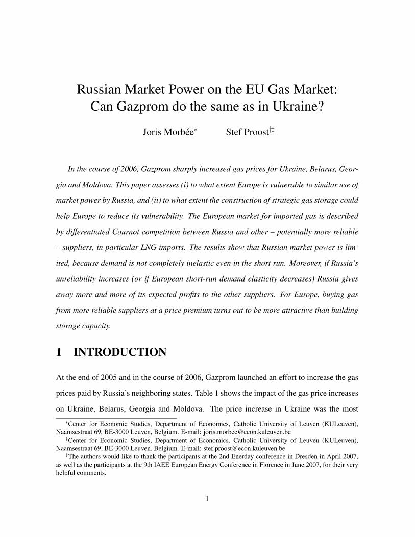
Russian Market Power on the EU Gas Market:Can Gazprom do the same as in Ukraine?
Joris Morbee∗ Stef Proost†‡
In the course of 2006, Gazprom sharply increased gas prices for Ukraine, Belarus, Geor-
gia and Moldova. This paper assesses (i) to what extent Europe is vulnerable to similar use of
market power by Russia, and (ii) to what extent the construction of strategic gas storage could
help Europe to reduce its vulnerability. The European market for imported gas is described
by differentiated Cournot competition between Russia and other – potentially more reliable
– suppliers, in particular LNG imports. The results show that Russian market power is lim-
ited, because demand is not completely inelastic even in the short run. Moreover, if Russia’s
unreliability increases (or if European short-run demand elasticity decreases) Russia gives
away more and more of its expected profits to the other suppliers. For Europe, buying gas
from more reliable suppliers at a price premium turns out to be more attractive than building
storage capacity.
1 INTRODUCTION
At the end of 2005 and in the course of 2006, Gazprom launched an effort to increase the gas
prices paid by Russia’s neighboring states. Table 1 shows the impact of the gas price increases
on Ukraine, Belarus, Georgia and Moldova. The price increase in Ukraine was the most
∗Center for Economic Studies, Department of Economics, Catholic University of Leuven (KULeuven),Naamsestraat 69, BE-3000 Leuven, Belgium. E-mail: [email protected]
†Center for Economic Studies, Department of Economics, Catholic University of Leuven (KULeuven),Naamsestraat 69, BE-3000 Leuven, Belgium. E-mail: [email protected]
‡The authors would like to thank the participants at the 2nd Enerday conference in Dresden in April 2007,as well as the participants at the 9th IAEE European Energy Conference in Florence in June 2007, for their veryhelpful comments.
1
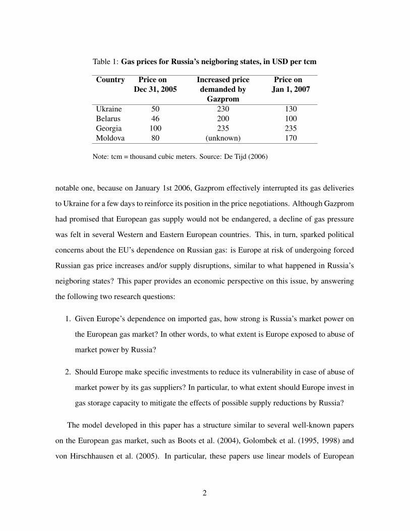
Table 1: Gas prices for Russia’s neigboring states, in USD per tcm
Country Price onDec 31, 2005
Increased pricedemanded by
Gazprom
Price onJan 1, 2007
Ukraine 50 230 130Belarus 46 200 100Georgia 100 235 235Moldova 80 (unknown) 170
Note: tcm = thousand cubic meters. Source: De Tijd (2006)
notable one, because on January 1st 2006, Gazprom effectively interrupted its gas deliveries
to Ukraine for a few days to reinforce its position in the price negotiations. Although Gazprom
had promised that European gas supply would not be endangered, a decline of gas pressure
was felt in several Western and Eastern European countries. This, in turn, sparked political
concerns about the EU’s dependence on Russian gas: is Europe at risk of undergoing forced
Russian gas price increases and/or supply disruptions, similar to what happened in Russia’s
neigboring states? This paper provides an economic perspective on this issue, by answering
the following two research questions:
1. Given Europe’s dependence on imported gas, how strong is Russia’s market power on
the European gas market? In other words, to what extent is Europe exposed to abuse of
market power by Russia?
2. Should Europe make specific investments to reduce its vulnerability in case of abuse of
market power by its gas suppliers? In particular, to what extent should Europe invest in
gas storage capacity to mitigate the effects of possible supply reductions by Russia?
The model developed in this paper has a structure similar to several well-known papers
on the European gas market, such as Boots et al. (2004), Golombek et al. (1995, 1998) and
von Hirschhausen et al. (2005). In particular, these papers use linear models of European
2
demand, and analyze supplier profits under different market structures1. Von Hirschhausen et
al. (2005) analyze profits and market power of transportation countries such as Ukraine, while
Boots et al. (2004) and Golombek et al. (1995, 1998) analyze the impact of changes on the
demand side, such as liberalization and trading. The set-up of this paper is also related to the
hold-up literature, as in Hubert and Ikonnikova (2004) for instance. Contrary to typical hold-
up papers, this paper considers the situation in which consumers are held up by a supplier
instead of the other way around. Indeed, once the consumers have decided on the gas quan-
tities from different suppliers, they are limited to the capacity of the production and transport
infrastructure agreed with each supplier. When one supplier decreases production, production
from other suppliers cannot be increased quickly, and so this supplier can increase his price to
monopoly levels by deliberately reducing supply. For that reason, this paper is also related to
the literature on long-term gas contracts, such as Boucher et al. (1987) and Neuhoff and von
Hirschhausen (2005).
On a broader microeconomic level, the analysis of this paper fits into the literature on
differentiated duopoly. Indeed, as will be shown in section 2, the contrast of a potentially un-
reliable gas supplier (in this case: Russia) and a reliable supplier (in this case: the other sup-
pliers, in particular through LNG), results in a market structure very similar to a differentiated
duopoly. Singh and Vives (1984) for example, compare Cournot and Bertrand competition in
differentiated duopoly, while Gaudet and Moreaux (1990) do the same for the particular case
of nonrenewable natural resources. The main contribution of our paper is that it introduces
the notion of risk directly into the market structure of the European gas market, and that it in-
corporates risk aversion of European consumers. Similar to the pioneering paper of Nordhaus
(1974), who analyzes oil supply interruptions, there are two regimes: a normal regime and a
supply interruption regime, each with its probability. As in Nordhaus (1974), the option of
storage is investigated2. However, in addition, the model of this paper analyzes the contrast
1However, unlike this paper, the models of Boots et al. (2004) and Golombek et al. (1995, 1998) analyze asegmentation of the European market, based on country and/or type of consumer.
2Nordhaus (1974) investigates also import taxes, but it turns out that storage is the most specific response tosupply security concerns. In this paper, storage shall therefore be used as the exemplification of a broader range
3
between an unreliable supplier and a reliable supplier. In this setting, gas purchases from a
reliable supplier serve as a substitute for storage.
The paper is organized as follows. First, section 2 describes the model used and the
computation of equilibria. Section 3 starts with the calibration of the model and proceeds
with the presentation of numerical simulations and sensitivities. Finally, section 4 returns to
the initial research questions.
2 MODEL OF THE EUROPEAN IMPORTED GAS MAR-KET
2.1 Overview of the game
The model in this paper describes the European imported gas market. More specifically, the
good considered is gas imported into Europe from non-European suppliers, delivered to the
border of a large Western European country3. The 3 key players in this market are (i) Europe,
(ii) Russia, and (iii) the other non-European gas suppliers on the European market (these
suppliers are lumped together and will be called other suppliers, for the sake of conciseness).
Europe is modelled as a large number of uncoordinated gas consumers, with an overarch-
ing government. The role of this ‘European government’ is limited to one policy instrument: it
can decide upfront how much storage will be built to protect Europe against potential Russian
supply shocks. The assumption that the storage decision is made by a European government
(as opposed to national governments) is inspired by the European interest in strategic gas
storage, as described in a recent communication of the European Commission (2007). Gas
purchase decisions are not made by the government, but by the individual gas consumers.
These consumers decide which quantities to buy from each supplier, taking into account the
storage built by the government. Since there is no coordination between the many European
of policy measures.3This focus has two simplifying implications: first, the price includes transportation costs up to the border
but does not consider local distribution to the European end consumer. Secondly, since the model only dealswith imported gas, the model does not consider any strategic behavior of European suppliers such as the UK orNorway.
4
gas buyers, they are considered to be price-takers. Furthermore, European gas consumers are
assumed to be risk-averse: they prefer a deterministic amount of consumer surplus, rather than
a ‘lottery’ between a lower and a higher amount, even when the expected value of the lottery
is as high as the certain amount. The consumers’ risk aversion is also taken into account by
the government when it makes decisions about building gas storage4.
Russia is modelled as a monolithic entity, i.e. no difference is made between the Russian
state and the gas producer Gazprom. Russia is assumed to be a risk-neutral profit maximizer.
Russia is modelled to be unreliable: in the last stage of the game, there is a probablity δ that
Russia does not stick to its previous supply commitments, i.e., Russia ‘defaults’. Conversely,
there is a probability (1 − δ) that Russia honors its commitments. The exact assumptions of
Russia’s behavior are explained later in this section.
The other suppliers are also modelled as one monolithic profit maximizer5. They are
assumed to be completely reliable, meaning that they always deliver the promised quantity of
gas at the promised price. The assumption of reliability is a strong one, but it can be justified
because non-Russian gas will increasingly be imported through LNG, which is costly but
offers diversified – and hence more reliable – access to a large range of potential gas sources.
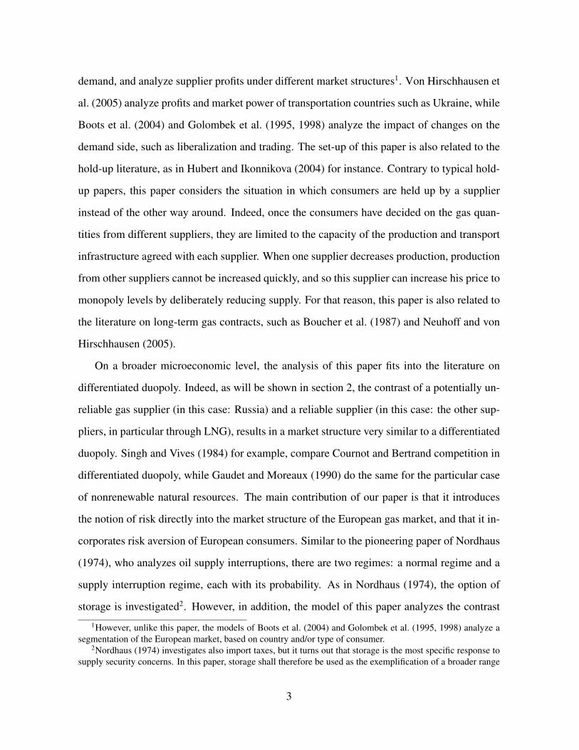
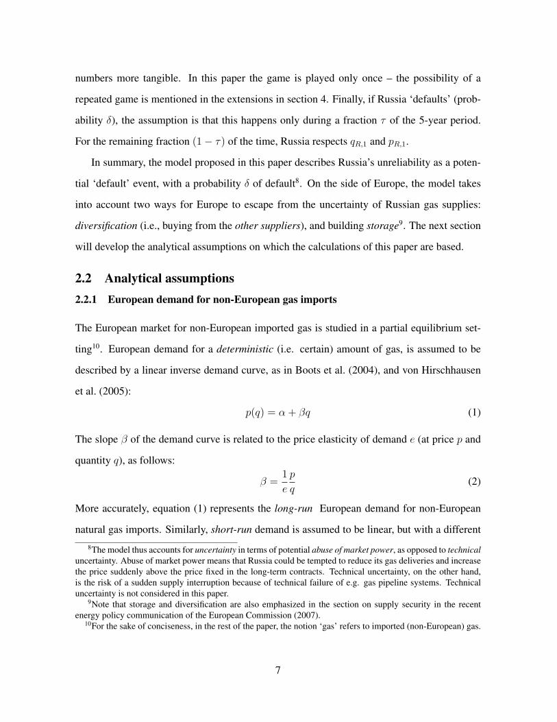
The interaction between the three players is modelled as a game in three stages. Figure 1
explains the different stages of the model.
In stage 1, the European government decides to foresee a quantity qS (in bcm, i.e., billion
cubic meters) of gas storage, to be used as a buffer in case of supply interruptions from Russia.
In stage 2, Russia and the other suppliers put gas on the European market. Russia puts a
quantity qR,1 (in bcm) on the European market, and receives a price pR,1 (in EUR per tcm, i.e.,
EUR per thousand cubic meters) for it6. The other suppliers put a quantity q0 (in bcm) on the
4For the sake of conciseness, throughout the paper, the term ‘Europe’ shall be used to denote both the Eu-ropean government and the European consumers, without risk of confusion. Expressions like “Europe buildsstorage X” and “Europe buys quantity Y” will thus be used as short-hand for “the European government decidesto build storage X” and “European consumers buy quantity Y”, respectively.
5No assumption needs to be made regarding the risk attitude of the other suppliers, since in this model theyare not confronted with any non-deterministic events.
6Note that bcm is consistently used for quantities, while EUR / tcm is consistently used for price. Thealternative use of bcm and tcm makes the resulting quantity and price numbers end up conveniently in the 0-300
5
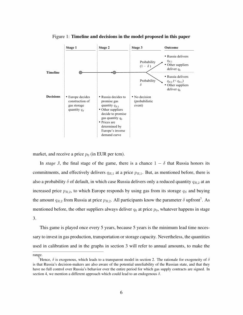
Figure 1: Timeline and decisions in the model proposed in this paper
Timeline
Decisions
Stage 1 Stage 2 Stage 3 Outcome
• Europe decides construction of gas storage quantity qS
Probability(1 – δ )
Probabilityδ
• Russia decides to promise gas quantity qR,1
• Other suppliers decide to promise gas quantity q0
• Prices are determined by Europe’s inverse demand curve
• No decision (probabilistic event)
• Russia delivers qR,1
• Other suppliers deliver q0
• Russia delivers qR,2 (< qR,1)
• Other suppliers deliver q0
market, and receive a price p0 (in EUR per tcm).
In stage 3, the final stage of the game, there is a chance 1 − δ that Russia honors its
commitments, and effectively delivers qR,1 at a price pR,1. But, as mentioned before, there is
also a probability δ of default, in which case Russia delivers only a reduced quantity qR,2 at an
increased price pR,2, to which Europe responds by using gas from its storage qS and buying
the amount qR,2 from Russia at price pR,2. All participants know the parameter δ upfront7. As
mentioned before, the other suppliers always deliver q0 at price p0, whatever happens in stage
3.
This game is played once every 5 years, because 5 years is the minimum lead time neces-
sary to invest in gas production, transportation or storage capacity. Nevertheless, the quantities
used in calibration and in the graphs in section 3 will refer to annual amounts, to make the
range.7Hence, δ is exogenous, which leads to a transparent model in section 2. The rationale for exogeneity of δ
is that Russia’s decision-makers are also aware of the potential unreliability of the Russian state, and that theyhave no full control over Russia’s behavior over the entire period for which gas supply contracts are signed. Insection 4, we mention a different approach which could lead to an endogenous δ.
6
numbers more tangible. In this paper the game is played only once – the possibility of a
repeated game is mentioned in the extensions in section 4. Finally, if Russia ‘defaults’ (prob-
ability δ), the assumption is that this happens only during a fraction τ of the 5-year period.
For the remaining fraction (1− τ) of the time, Russia respects qR,1 and pR,1.
In summary, the model proposed in this paper describes Russia’s unreliability as a poten-
tial ‘default’ event, with a probability δ of default8. On the side of Europe, the model takes
into account two ways for Europe to escape from the uncertainty of Russian gas supplies:
diversification (i.e., buying from the other suppliers), and building storage9. The next section
will develop the analytical assumptions on which the calculations of this paper are based.
2.2 Analytical assumptions2.2.1 European demand for non-European gas imports
The European market for non-European imported gas is studied in a partial equilibrium set-
ting10. European demand for a deterministic (i.e. certain) amount of gas, is assumed to be
described by a linear inverse demand curve, as in Boots et al. (2004), and von Hirschhausen
et al. (2005):
p(q) = α + βq (1)
The slope β of the demand curve is related to the price elasticity of demand e (at price p and
quantity q), as follows:
β =1
e
p
q(2)
More accurately, equation (1) represents the long-run European demand for non-European
natural gas imports. Similarly, short-run demand is assumed to be linear, but with a different
8The model thus accounts for uncertainty in terms of potential abuse of market power, as opposed to technicaluncertainty. Abuse of market power means that Russia could be tempted to reduce its gas deliveries and increasethe price suddenly above the price fixed in the long-term contracts. Technical uncertainty, on the other hand,is the risk of a sudden supply interruption because of technical failure of e.g. gas pipeline systems. Technicaluncertainty is not considered in this paper.
9Note that storage and diversification are also emphasized in the section on supply security in the recentenergy policy communication of the European Commission (2007).
10For the sake of conciseness, in the rest of the paper, the notion ‘gas’ refers to imported (non-European) gas.
7
slope βSR. So the short-run demand variations around a long-run equilibrium (p∗, q∗) are
given by:
pSR(q) = p∗ + βSR(q − q∗) (3)
with βSR related to the short-run elasticity eSR just like in (2). k is defined as the ratio βSR/β
between long-run and short-run elasticity.
The description above refers to European demand for a certain (i.e. deterministic) gas
quantity and price, and is fairly common. However, since Europe is risk-averse it is impor-
tant to model how Europe deals with an uncertain gas quantity and/or price. Following the
theory of expected utility, a straightforward way of modelling Europe’s risk aversion is by
transforming Europe’s pay-offs using a concave function u(·), before maximizing Europe’s
expected utility. Europe’s pay-off for a deterministic gas quantity q at price p is its consumer
surplus CS:
CS =
∫ q
0
p(x)dx− pq = αq +1
2βq2 − pq (4)
In expected utility theory, Europe’s risk-averse decision-making can be modelled by maximiz-
ing the expected value E[U ], where U = u(CS) is a concave transformation of CS. The most
transparent choice of u(·) is a function that yields constant relative risk aversion (CRRA):
u(x) = uθ(x) =x1−θ
1− θ(5)
where θ is the coefficient of relative risk aversion. For θ = 0, E[U ] = E[CS] and Europe is
risk-neutral. For θ > 0, Europe becomes more and more risk-averse. Equivalent to maximiz-
ing E[U ], Europe can maximize the certainty equivalent Cθ:
Cθ = u−1θ (E[U ]) = u−1
θ (E[uθ(CS)]) (6)
Cθ from equation (6) is used in this paper to model Europe’s decision process. In the rest of
the paper, the term consumer surplus refers to CS (interpreted as in equation (4)), while utility
refers to U and certainty equivalent refers to Cθ.
8
2.2.2 Production, transportation and storage costs
Marginal costs for gas production are assumed to be constant: cR for Russia, and c0 for the
other suppliers. These marginal costs are to be interpreted as long-run marginal costs, i.e.,
they include investments needed for maintaining or expanding the production. Hence, it is
sound to express total production costs for Russia as qR · cR (for a quantity qR), and, similarly,
to express total production costs for the other suppliers as q0 · c0 (for a quantity q0)11.
As mentioned in section 2.1, the model assumes that delivery to the border of a large
Western European country is contained in the price of the gas. Therefore, transportation costs
should be included in the production costs. In Boots et al. (2004), Golombek et al. (1995,
1998) and von Hirschhausen et al. (2005), transportation is modelled as having a constant
cost per tcm. The constant depends on the distance, and hence on the supplying country.
Therefore, in this analysis, the transportation costs can be included in the constants cR and c0.
The term transportation costs is to be understood as the costs to transport the gas from the
production site to the border of Germany (for Russian gas) or France (for the other suppliers,
because marginal supply is likely to be imported through LNG). Since this paper analyzes the
gas market on an aggregated European level, the distribution costs (to deliver the gas to the
end consumer), are not considered.
As described in Mulder and Zwart (2006), the storage costs for natural gas can be de-
scribed as a constant cS , which gives the annual cost per unit of gas storage capacity. The
total annual cost to provide storage for a quantity qS is then qS · cS .11While it is analytically convenient to describe the marginal production costs of Russia and the other suppliers
as constants cR and c0, it is a simplification of the long-term physical reality: as production increases, newproduction sites will inevitably be less accessible and more costly to exploit. A more refined way of modellingmarginal production costs is used by Boots et al. (2004) and Golombek et al. (1995, 1998):
MCproduction = a + bq + c ln(1− q/Q) (7)
where q is production and Q is capacity (the third term makes production costs go up to infinity as soon ascapacity is reached). The constants a, b, c and Q are determined for each supplier country separately. The exactvalues of a, b, c and Q are listed in Golombek et al. (1995), and are the same in the three studies Boots et al.(2004) and Golombek et al. (1995, 1998). For Russia however, b is 0, which is in line with the assumptionof constant marginal cost used in this paper (except for the capacity constraint). As described later, marginalcosts for the other suppliers are taken from Qatar, a country with very large gas production potential at relativelyconstant marginal cost, so that the assumption of constant marginal costs for the other suppliers is again justified.
9
2.3 Solution
We now analyze the game described in section 2.1, using backward induction.
2.3.1 Stage 3
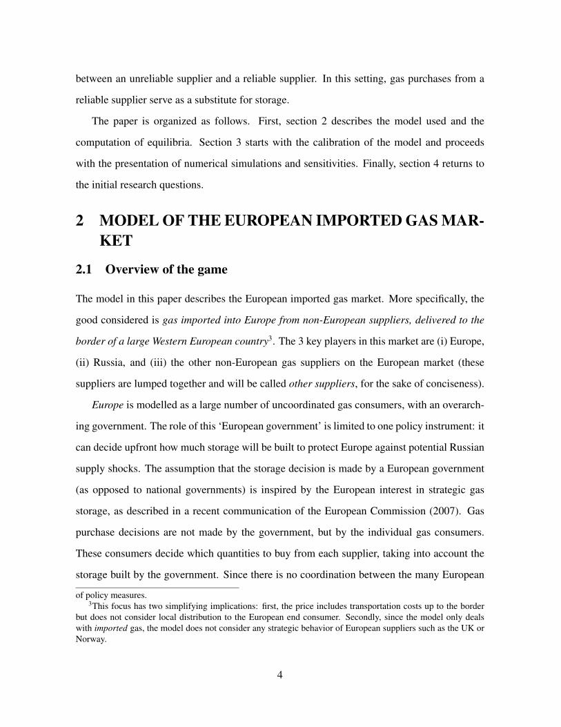
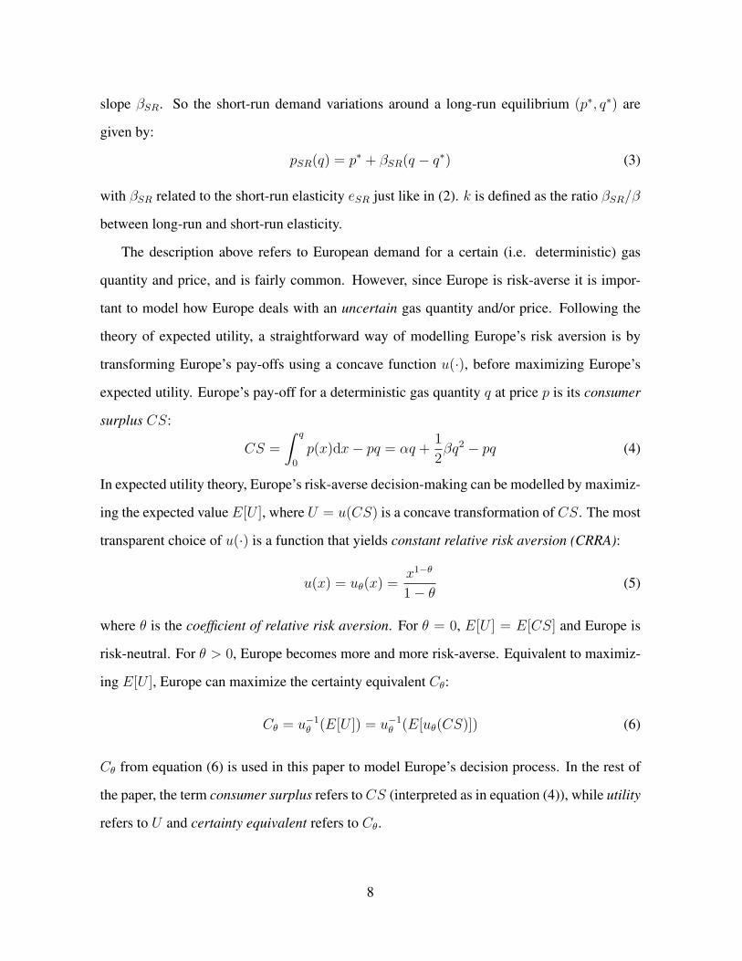
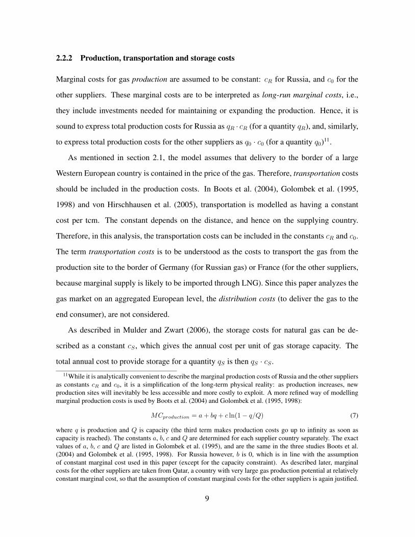
Case 1: Russia honors its commitments. In this case, the European consumer surplus is
given by:
CS1 = α · (q0 + qR,1) +1
2β · (q0 + qR,1)
2 − p0q0 − pR,1qR,1 − cSqS (8)
This follows from equation (4), or directly graphically from figure 2. Note that the storage
cSqS has to be paid even though the storage is not used in this case. Russia’s profits are:
ΠR,1 = (pR,1 − cR) · qR,1 (9)
Figure 2: Demand and supply in case 1:Russia honours its commitments.
p
q
p0
q0 q0 + qR,1
pR,1
p(q) = α + β qCS1
Figure 3: Demand and supply in case 2:Russia defaults.
p
q
p0
q0
pR,1
pSR (q) =
pR
,1+
β(q-q
0 -qR
,1 )
q0 + qR,1
qS qR,2
pR,2
p(q) = α + β q
Case 2: Russia defaults. In this case, Russia does not supply qR,1 at pR,1, but delivers
a lower quantity qR,2 at a higher price pR,2, because of monopolistic profit maximization12.
12As mentioned in section 2.1, Russia cheats only during a fraction τ of the 5-year time period. However, forthe clarity of the presentation, τ is assumed to be 100% throughout section 2, and shall be reintroduced as ofsection 3.
10
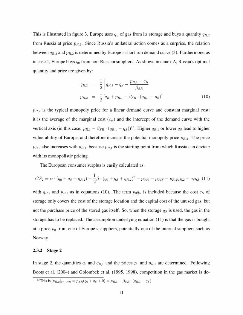
This is illustrated in figure 3. Europe uses qS of gas from its storage and buys a quantity qR,2
from Russia at price pR,2. Since Russia’s unilateral action comes as a surprise, the relation
between qR,2 and pR,2 is determined by Europe’s short-run demand curve (3). Furthermore, as
in case 1, Europe buys q0 from non-Russian suppliers. As shown in annex A, Russia’s optimal
quantity and price are given by:
qR,2 =1
2
[qR,1 − qS −
pR,1 − cR
βSR
]pR,2 =
1
2[cR + pR,1 − βSR · (qR,1 − qS)] (10)
pR,2 is the typical monopoly price for a linear demand curve and constant marginal cost:
it is the average of the marginal cost (cR) and the intercept of the demand curve with the
vertical axis (in this case: pR,1 − βSR · (qR,1 − qS))13. Higher qR,1 or lower qS lead to higher
vulnerability of Europe, and therefore increase the potential monopoly price pR,2. The price
pR,2 also increases with pR,1, because pR,1 is the starting point from which Russia can deviate
with its monopolistic pricing.
The European consumer surplus is easily calculated as:
CS2 = α · (q0 + qS + qR,2) +1
2β · (q0 + qS + qR,2)
2 − p0q0 − p0qS − pR,2qR,2 − cSqS (11)
with qR,2 and pR,2 as in equations (10). The term p0qS is included because the cost cS of
storage only covers the cost of the storage location and the capital cost of the unused gas, but
not the purchase price of the stored gas itself. So, when the storage qS is used, the gas in the
storage has to be replaced. The assumption underlying equation (11) is that the gas is bought
at a price p0 from one of Europe’s suppliers, potentially one of the internal suppliers such as
Norway.
2.3.2 Stage 2
In stage 2, the quantities q0 and qR,1 and the prices p0 and pR,1 are determined. Following
Boots et al. (2004) and Golombek et al. (1995, 1998), competition in the gas market is de-13This is [pR,2]qR,2=0 = pSR(q0 + qS + 0) = pR,1 − βSR · (qR,1 − qS)
11
scribed using the Cournot model, in which quantities are the strategic variables14. This means
that Russia and the other suppliers simultaneously determine the supplied quantities q0 and
qR,1. The prices p0 and pR,1 then arise from the response of European demand to the supplied
quantities q0 and qR,1.
The first step to compute the Cournot equilibrium is to determine the European demand
curve. For given prices p0 and pR,1, European demand is derived from the expected utility in
stage 3. If Europe were risk-neutral, the expected utility in stage 3 would be nothing more
than the expected consumer surplus E[CS]:
E[CS] = (1− δ) · CS1 + δ · CS2 (12)
with CS1 and CS2 calculated as in (8) and (11). For a risk-neutral Europe, the quantities
demanded at prices p0 and pR,1 would be the quantities q0 and qR,1 that maximize equation
(12). However, as discussed in section 2.2.1, Europe is risk-averse, and so the demand should
be derived from the certainty equivalent Cθ, i.e. from equation (6) rather than from equation
(12). Annex B shows that with a number of simplifying assumptions, Cθ can be approximated
by a formula that is analytically as convenient as (12):
Cθ ≈ (1− σ) · CS1 + σ · CS2 (13)
with σ defined as in:
σ = δ +1
2δ(1− δ)θA with A =
CS1 − CS2
CS1
(14)
This approximation has the advantage of having a very intuitive interpretation: in equation
(13), Europe ‘perceives’ a Russian default probability σ, which is different from the ‘real’14An intuitively appealing alternative is the Bertrand model, in which prices are the strategic variables: in
that case, Russia and the other suppliers would set prices p0 and pR,1, and European demand would respond bydeciding which quantities q0 and qR,1 it would consume at the given prices p0 and pR,1. The Bertrand modelis intuitively appealing because e.g. the conflict between Russia and Ukraine in January 2006 was about gasprice. However, as mentioned in section 2.1, the lead times for investments in production and transportationcapacity in the gas market are rather long. So, even if there is competition with price as strategic variable, thecompetition can only take place within the boundaries of the capacity constraints. However, according to Krepsand Scheinkman (1983), a 2-stage game in which players choose capacities in the first stage and do Bertrandcompetition in the second stage, is equivalent to Cournot competition.
12
default probability δ. Europe’s risk aversion is thus modelled as a higher perceived default
probability15. Indeed, for the cases δ = 0 and δ = 1, there is no uncertainty, so σ = δ. The
more uncertainty (i.e. the closer to δ = 0.5), the larger the difference between σ and δ.
Based on the formula for Cθ, European demand for imported gas from Russia and other
suppliers can be determined by finding the optimal (q0, qR,1) that maximize Cθ for given p0
and pR,1, subject to16:
α + β(q0 + qR,1) = pR,1 (15)
Practically, equation (15) is easily solved for qR,1 and then substituted in equation (13). Next,
the optimal q0 can be determined analytically by maximizing Cθ. For the special case in which
βSR = β, the result is:
q0 =4
3
1
σβp0 −
1
3
4− 4σ
σβpR,1 −
1
3
3σα + 3σβqS + σcR
σβ(16)
Retaking equation (15) and solving (16) for p0, gives the following inverse demand curves:
p0 =4α− ασ + σcR + 3σβqS
4+
4− σ
4βq0 + (1− σ)βqR,1
pR,1 = α + βq0 + βqR,1 (17)
These are the inverse demand curves for a differentiated duopoly: because of the Russian
uncertainty, the one-good gas sector is transformed into a two-good sector. Since β < 0 and
0 ≤ σ ≤ 1, the partial derivatives ∂p0/∂q0, ∂p0/∂qR,1, ∂pR,1/∂q0 and ∂pR,1/∂qR,1 are all
negative, as is expected for substitute goods. A quick check is that for σ = 0 there is no
more differentiation between the two suppliers, and equations (17) reduce to equation (1).
15The caveat is that σ is actually not a constant, but depends on A, which is the proportional ‘deviation’between CS1 and CS2. However, in addition to the approximations made in annex B, σ will be treated as aconstant in subsequent analyses. σ will therefore change with δ as defined in equation (14), but will not dependon CS1 and CS2, because a fixed A is taken.
16The condition (15) needs to be applied explicitly. If not, the total quantity q0 + qR,1 may be less than thequantity needed to satisfy all European demand at the price pR,1. The reason is that Europe would deliberatelycut back gas imports to stop itself from becoming too dependent. Indeed, by cutting back qR,1, Europe obtainsa better ‘location’ for its SR-demand curve in case Russia defaults. However, it seems unrealistic that in theever more liberalized European gas market, there would be unsatisfied demand, i.e., rationing, at the price pR,1.Rationing is an entirely different policy instrument and is not considered here. Therefore, the assumption ismade that q0 and qR,1 always jointly satisfy all the demand at pR,1.
13
In the numerical simulations of section 3, βSR will be different from β, giving rise to more
complicated formulas than (17).
In the Cournot model, Russia and the other suppliers set quantities q0 and qR,1 as strategic
variables. Taking into account Europe’s inverse demand curves (17), Russia and the other
suppliers try to maximize their expected profits, ΠR and Π0, respectively:
ΠR = (1− δ)ΠR,1 + δΠR,2
Π0 = (p0 − c0) · q0 (18)
Recall that ΠR,1 and ΠR,2 are Russia’s profits in cases 1 and 2, respectively, and that Russian
policy is risk-neutral. Russia and the other suppliers could maximize their expected profits
either cooperatively (as in a cartel) or non-cooperatively. Following Boots et al. (2004) and
Golombek et al. (1995, 1998), this paper assumes that Russia and the other non-European
suppliers reach the non-cooperative (Nash) equilibrium, as in the traditional Cournot model.
Hence, suppliers choose quantities so that each player’s quantity maximizes his own profits
given the other player’s quantity. The resulting quantities (q0, qR,1) and corresponding prices
(according to equations (17)) can be expressed analytically, but the result is long and not very
insightful.
2.3.3 Stage 1
Substituting the calculated equilibrium quantities and prices into (13) and maximizing for qS
yields an optimal amount of gas storage capacity qS . It can also be expressed analytically.
Note that qS is chosen before q0 and qR,1, as in a Stackelberg leadership model.
3 NUMERICAL RESULTS
3.1 Calibration
This section describes the numerical assumptions for the parameters used in our model. These
values are based on estimates from the literature:
14
Demand. The parameters α, β and βSR were determined using elasticities from the literature,
and the 2005 baseline in terms of volume and price. Long-run price elasticity of demand
was taken equal to -0.93, following Golombek et al. (1998). Short-run price elasticity
of demand was determined based on the very comprehensive literature survey of Dahl
(1993). In Dahl (1993), the average short-run elasticity over the 15 studies that com-
pute both short-run and long-run elasticities was -0.2717. According to BP (2006), the
volume of non-European gas imports in 2005 was 213 bcm (mostly from Russian and
Algerian pipelines, and LNG). The average BAFA-price (i.e., the German border price
as registered by the German Bundesministerium fur Wirtschaft und Technologie, see
BAFA, 2006) was 138.9 EUR per tcm in 2005. Based on these numbers, the resulting
β, βSR and, finally, α can be determined.
Costs. Total per-unit production and transportation costs c0 and cR are taken from OME
(2002), which shows costs curves for additional volumes of gas supply to the EU-15
in 2010. For Russia, we based the marginal costs on production in the Nadym-Pur-
Taz region, with transport through Belarus ($2.3/MBtu, or 67 EUR/tcm18). For the
other suppliers, costs are based on LNG imports from Qatar and Iran ($3.0/MBtu or
87 EUR/tcm), because that region offers large future expansion potential. The annual
storage costs cS were taken in the middle of the range 50-70 EUR per tcm per year,
mentioned by Mulder and Zwart (2006).
Other. The approximative coefficient of relative risk aversion θ was chosen in line with a
Swedish survey by Palsson (1996), which computes a coefficient of 2 to 4 for financial
assets, and 10 to 15 when real assets are also included. The choice of θ = 8 is right in
the middle of this range. The value of A (the approximative percentage difference in
consumer surplus between the two cases) was set to 25%, which is generally consistent
with the output values of CS1 and CS2 in the simulations in section 3.2. Since the17Note that the average long-run elasticity of the same 15 studies was -0.99, which is in line with the -0.93
from Golombek et al. (1998).18USD/EUR conversions are done at the average exchange rate for the base year 2005 (1 USD = 0.80 EUR).
15
parameter δ is crucial, it is subject of an extensive sensitivity analysis in section 3.2.1,
and otherwise it is chosen to be 15%. Parameter τ is assumed to be 50%. Recall that τ
is the fraction of the 5-year time period, during which Russia cheats – if it cheats at all.
So, for instance, with τ = 50% and δ = 15%, there is a 15% chance that Russia does
monopolistic pricing during 2.5 years out of the total 5 years, while there is an 85%
chance that Russia does not cheat at all during the 5-year period.
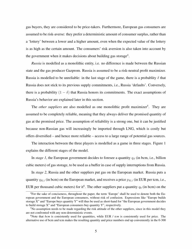
3.2 Simulations and interpretation3.2.1 Effect of the default probability δ
The top half of figure 4 shows how quantities and prices vary as δ goes from 0 to 1. (Recall
that δ is the probability that Russia does not fulfil its contractual obligations.) The graph also
shows the price difference ∆p between Russian and other gas (∆p = p0 − pR,1).
For δ = 0, there is no risk and there is obviously no price difference between Russian and
other gas. The simulation shows that in this case, Europe buys qR,1 = 115 bcm from Russia
and q0 = 86 bcm from the other suppliers. This is relatively close to the actual data as cited
by BP (2006), which mentions 122 bcm from Russia and 91 bcm from other non-European
suppliers.
When δ > 0, Russia becomes unreliable. If Russia ‘defaults’, it produces only qR,2 instead
of qR,1, at a higher price pR,2 instead of the original contracted price pR,1. However, figure 4
shows that this would not imply a total interruption or a fourfold price increase, as it happened
in Ukraine. The volume reduction would rather be around 1/3, and would bring about a price
increase of 2/3, which is only slightly higher than seasonal variations observed at European
hubs like Zeebrugge. As δ increases, the other suppliers sell more and more gas q0 to Europe,
at a slowly increasing price p0. Meanwhile, Russia also sells an increasing amount qR,1 to
Europe, even though Russia is obliged to give a steeply increasing discount ∆p to be able to
sell this increasing amount of gas to Europe. It is obvious why Russia would want to do this:
as δ increases, there is a higher chance that Russia can charge the monopoly price pR,2 in stage
16
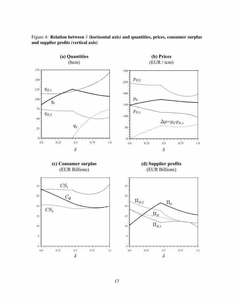
Figure 4: Relation between δ (horizontal axis) and quantities, prices, consumer surplusand supplier profits (vertical axis)
δ
(a) Quantities(bcm)
(b) Prices(EUR / tcm)
(c) Consumer surplus(EUR Billions)
(d) Supplier profits(EUR Billions)
δ
δ δ
qR,1
qR,2
q0
qS
pR,2
pR,1
p0
∆p =p0-pR,1
CS1
CS2
CθΠ0
ΠR,1
ΠR,2
ΠR
17
3 (by producing only a quantity qR,2 of gas). By giving a large discount ∆p, Russia can induce
Europe to buy more qR,1 (despite the uncertainty), which puts Europe in a vulnerable situation.
Indeed, even though Europe buys more and more ‘safe’ gas q0, the potential monopoly price
pR,2 and quantity qR,2 are hardly affected, precisely because Russia sells enough qR,1 to make
sure that Europe’s SR-demand curve is far enough out to the right (see figure 3).
At some point, when δ = 0.45, the situation becomes so risky for Europe, that storage
qS becomes competitive. As of that point, the amount of gas bought from other suppliers q0,
and the associated price p0, start to go down because the safe gas is being ‘substituted’ by
storage qS . Because of the increasing storage capacity, pR,2 (Russia’s potential ‘monopoly
price’) drops quite steeply. As a result, the Russian discount ∆p does not have to increase
as before to convince Europe to buy more qR,1. Finally, as δ approaches 1, there is no more
uncertainty: Europe knows for sure that Russia will cheat, but Europe is adequately prepared
with a balanced amount of qS and q0.
The bottom part of figure 4 shows the effect on Europe’s consumer surplus and certainty
equivalent, and on the suppliers’ profits. Recall that CS1 is Europe’s consumer surplus in case
1 (i.e., when Russia sticks to the contract), while CS2 is Europe’s consumer surplus in case 2
(i.e., when Russia defaults). As before, Cθ is the certainty equivalent of the lottery between
CS1 and CS2. For δ = 0, the certainty equivalent Cθ = CS1. For δ = 1, Cθ = CS2. In
between, Cθ is a weighted average of U1 and U2, with weights (1 − σ) and σ respectively.
When δ increases, Cθ decreases: for a risk-averse agent like Europe, increased uncertainty
leads to value destruction. As δ approaches 1, uncertainty decreases, and there is a very small
uptick in Europe’s certainty equivalent consumer surplus.
Panel (d) shows that Russia’s profits decrease monotonically with increasing δ. With
increasing δ, the gap between the profit ΠR,1 in case 1 and the profit ΠR,2 in case 2 initially
grows wider: Russia gives an ever steeper discount on its gas qR,1 to get a chance to obtain
the monopolistic profits ΠR,2. The only party who gains from increased uncertainty, are the
other suppliers. Their profits Π0 increase with increasing δ, because the increased uncertainty
18
gives them the opportunity to extract value from Europe’s risk aversion by offering a safer
solution. However, when δ grows larger than 0.45, they get competition from the storage
option. Because of this competition, and because uncertainty decreases when δ gets close to
1, the profits Π0 decrease between δ = 0.45 and δ = 1.
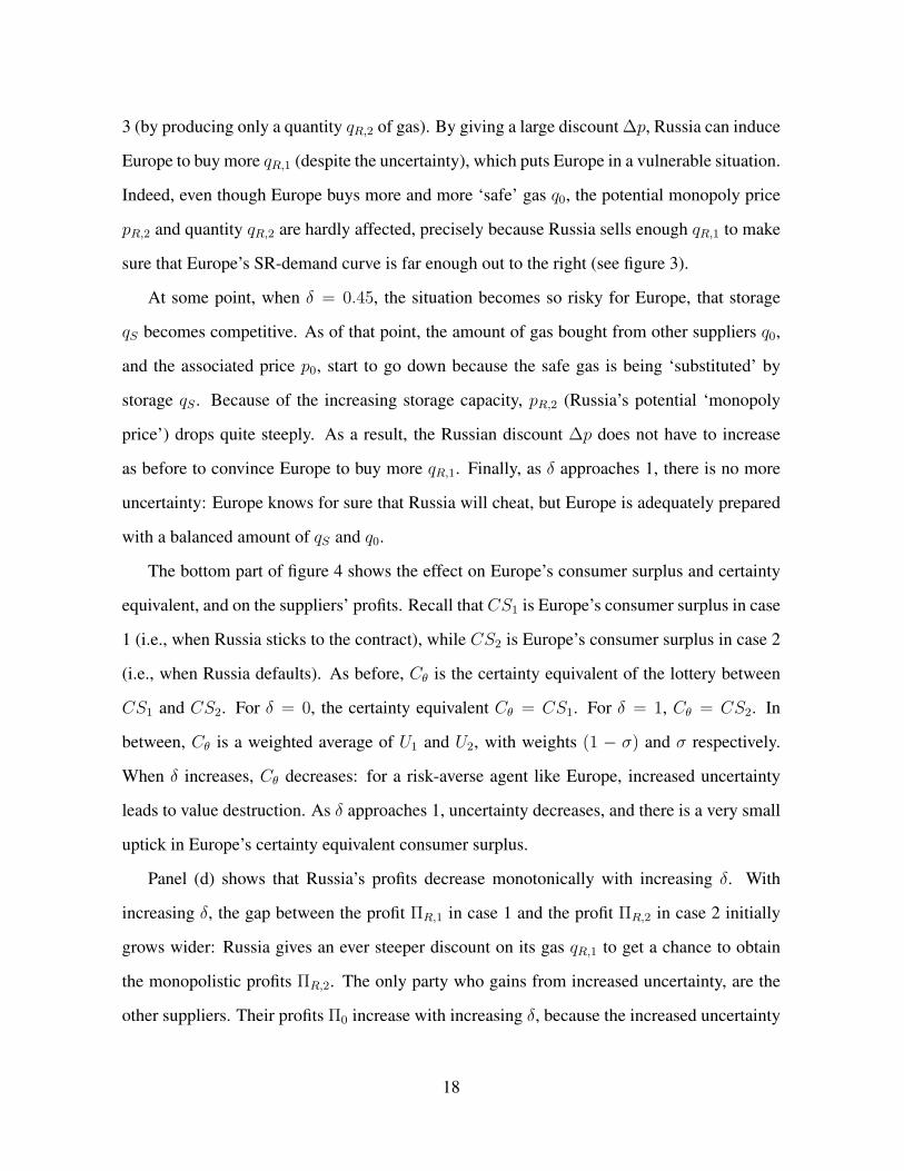
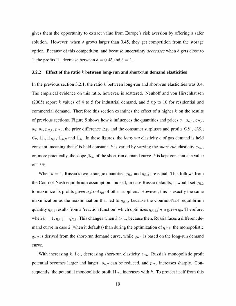
3.2.2 Effect of the ratio k between long-run and short-run demand elasticities
In the previous section 3.2.1, the ratio k between long-run and short-run elasticities was 3.4.
The empirical evidence on this ratio, however, is scattered. Neuhoff and von Hirschhausen
(2005) report k values of 4 to 5 for industrial demand, and 5 up to 10 for residential and
commercial demand. Therefore this section examines the effect of a higher k on the results
of previous sections. Figure 5 shows how k influences the quantities and prices q0, qR,1, qR,2,
qS , p0, pR,1, pR,2, the price difference ∆p, and the consumer surpluses and profits CS1, CS2,
Cθ, Π0, ΠR,1, ΠR,2 and ΠR. In these figures, the long-run elasticity e of gas demand is held
constant, meaning that β is held constant. k is varied by varying the short-run elasticity eSR,
or, more practically, the slope βSR of the short-run demand curve. δ is kept constant at a value
of 15%.
When k = 1, Russia’s two strategic quantities qR,1 and qR,2 are equal. This follows from
the Cournot-Nash equilibrium assumption. Indeed, in case Russia defaults, it would set qR,2
to maximize its profits given a fixed q0 of other suppliers. However, this is exactly the same
maximization as the maximiziation that led to qR,1, because the Cournot-Nash equilibrium
quantity qR,1 results from a ‘reaction function’ which optimizes qR,1 for a given q0. Therefore,
when k = 1, qR,1 = qR,2. This changes when k > 1, because then, Russia faces a different de-
mand curve in case 2 (when it defaults) than during the optimization of qR,1: the monopolistic
qR,2 is derived from the short-run demand curve, while qR,1 is based on the long-run demand
curve.
With increasing k, i.e., decreasing short-run elasticity eSR, Russia’s monopolistic profit
potential becomes larger and larger: qR,2 can be reduced, and pR,2 increases sharply. Con-
sequently, the potential monopolistic profit ΠR,2 increases with k. To protect itself from this
19
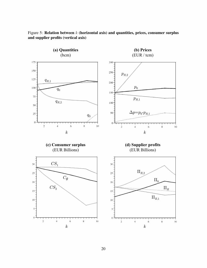
Figure 5: Relation between k (horizontal axis) and quantities, prices, consumer surplusand supplier profits (vertical axis)
k
(a) Quantities(bcm)
(b) Prices(EUR / tcm)
(c) Consumer surplus(EUR Billions)
(d) Supplier profits(EUR Billions)
k
k k
qR,1
qR,2
q0
qS
pR,2
pR,1
p0
∆p =p0-pR,1
CS1
CS2
Cθ Π0
ΠR,1
ΠR,2
ΠR
20
risk, Europe buys more q0 at a higher p0, thereby granting ever larger profits Π0 to the other
suppliers. Meanwhile, Russia sells more and more qR,1 at lower pR,1 (higher discount ∆p),
to make Europe dependent on Russian gas, and hence increase the potential for ΠR,2. All in
all, Russia’s expected profit ΠR actually decreases with k, a surprising result. The increased
vulnerability of Europe also leads to decreasing certainty-equivalent utility for Europe. The
winners of lower short-run elasticity are the reliable, other (non-Russian) suppliers. With
very high k, the risk for Europe grows so large that storage becomes a viable alternative. As
of k = 8.2, storage partly reverses the trends just described, although Cθ and ΠR are still
decreasing – but now also Π0 decreases.
3.2.3 Storage
In the simulations of figure 4, no storage capacity is built (qS = 0) when δ < 0.45. The annual
cost of storage, cS = 60 EUR per tcm, is high compared to the potential gains in that case.
Figure 6 shows for each value of δ the maximum value of cS for which qS > 0. The curve is
Figure 6: Relation between δ (horizontal axis) and maximum value of cS (in EUR / tcm)for which qS > 0 (vertical axis), for different values of risk aversion θ
θ=0
θ=8
θ=16
θ=24
cS=60
δ
21
plotted for different values of Europe’s risk aversion θ. There is storage investment qS > 0
in the region of the (δ, cS) space below the curve. In the graph, one can see that for θ = 8
(the value used in sections 3.2.1 and 3.2.2), the storage option becomes interesting only as of
δ = 0.45, as already seen in section 3.2.1. For moderate values of δ in the 0.1 to 0.2 range,
and θ = 8, storage costs of 60 EUR per tcm are 2-3 times too expensive to be attractive. When
Europe is more risk-averse – modelled by a higher θ – storage becomes attractive for values
of δ < 0.45, even at the cost of cS = 60 EUR per tcm.
4 CONCLUSIONS
The aim of this paper is to analyze the extent of Russia’s market power vis-a-vis European
consumers, and whether the construction of strategic storage would help Europe to reduce its
vulnerability. With the help of a partial equilibrium model of the imported gas market (as
described in section 2) and the numerical simulations of section 3, a number of interesting
conclusions can be reached.
First of all, Russia’s market power in the European gas market is limited. It is true that
Russia has the potential to suddenly increase prices and reduce gas deliveries to Europe. How-
ever, Russia is highly unlikely to cut off supplies completely, and in addition, an unreliable
attitude decreases Russia’s profits, while the other suppliers gain. Indeed:
• Russia will most likely not cut off supplies completely, or increase prices to unreason-
ably high levels. It would be much more profitable for Russia to suddenly increase
prices to the monopolistic price level, and reduce quantities accordingly. In the model
of this paper the profit-maximizing price increase is around 2/3, and it would coincide
with a quantity decrease of roughly 1/3. Raising prices even higher or reducing quanti-
ties even further is not attractive for Russia, because – even in the short term – European
demand for gas is elastic.
• Moreover, there is a serious downside for Russia if Europe perceives a high likelihood
that Russia will at some point in the future be tempted to charge the monopoly price.
22
For a default probability of only 15%, the model predicts that Russia needs to sell its gas
at a 13% discount (21 EUR per tcm), and that discount roughly doubles if the default
probability increases to 30%. As the default probability increases, Russia’s profits drop
monotonically because Europe purchases more gas from other suppliers, and builds
storage capacity to reduce the risk of short-term supply reductions.
• If the short-run elasticity of demand decreases further, Russia’s unreliability is even
more costly for Russia – a surprising result. True, a lower short-run elasticity offers
more profit potential for monopolistic quantity setting, but Europe anticipates this risk
by demanding a lower Russian price, buying more gas from other suppliers, and build-
ing storage capacity.
• Finally, if Russia starts monopolistic quantity and price setting, the chance that the other
suppliers jump on the bandwagon, is limited, because it is highly profitable to be the
reliable supplier: besides the significant price premium for reliable gas, any event that
highlights the unreliability of Russia will increase both the price and the quantity bought
from the reliable suppliers.
Secondly, in the model in this paper, storage is only attractive for Europe if Russian unreli-
ability is very high (more than 45% default probability), or if short-run demand becomes very
unelastic (more than ∼8 times as inelastic as long-term demand). In the other cases, buying
storage is less attractive than buying gas from the other, reliable, suppliers. Costs of storage
would typically need to be 2-3 times lower than their current value, for storage to become a
viable alternative instead of buying from reliable suppliers. At the same time, as pointed out
above, being reliable is a very profitable strategy for a supplier – so this is really a win-win
situation for Europe and the reliable supplier. The win-win potential exists, because reduc-
ing risk in the presence of a risk-averse party like Europe, eliminates a ‘deadweight loss’.
Building storage also reduces the risks, but entails unproductive investments and hence also a
loss.
23

A potential step for further research is to turn our model into a repeated game. In such
a game, δ could become endogenous as part of a mixed Russian strategy. Another poten-
tial extension is to model the impact on the downstream market, where high qR,1 could lead
to oversupply, but where there could be a distinction between risk-prone and risk-averse con-
sumers. Finally, this topic could be placed in a broader comparison of policy measures (import
taxes, rationing, etc.), and the discussion whether or not government intervention is needed
for e.g. storage construction.
ReferencesBAFA (2006). www.bafa.de, last consulted in October 2007.
Binmore, K. (1987). “Bargaining Models”, in R. Golombek, M. Hoel, and J. Vislie (eds.), Natural GasMarkets and Contracts, North Holland, Elsevier Science Publishers, 193-220.
Boots, M., F. Rijkers and B. Hobbs (2004). “Trading in the Downstream European Gas Market: ASuccessive Oligopoly Approach”, The Energy Journal 25(3): 73-102.
Boucher J., T. Hefting and Y. Smeers (1987). “Economic Analysis of Natural Gas Contracts”, in R.Golombek, M. Hoel, and J. Vislie (eds.), Natural Gas Markets and Contracts, North Holland, Else-vier Science Publishers, 193-220.
BP (2006). Statistical Review of World Energy June 2006, London, BP p.l.c.
Dahl, C. (1993). A Survey of Energy Demand Elasticities in Support of the Development of the NEMS,Paper prepared for United States Department of Energy, Contract De-AP01-93EI23499.
Commission of the European Communities (2007). An Energy Policy for Europe, Communication tothe European Council and the European Parliament.
Eyckmans, J. and S. Proost (1992). “Do we need an Oil Import Tax in Western Europe?”, Proceedingsof a meeting in 15th IAEE International Conference, Tours.
Gaudet, G. and M. Moreaux (1990). “Price versus Quantity Rules in Dynamic Competition: The Caseof Nonrenewable Natural Resources”, International Economic Review 31(3): 639-650.
Golombek R. and E. Gjelsvik (1995). “Effects of Liberalizing the Natural Gas Markets in WesternEurope”, The Energy Journal 16(1).
Golombek, R., E. Gjelsvik and K. Rosendahl (1998). “Increased Competition on the Supply Side ofthe Western European Natural Gas Market”, The Energy Journal 19(3): 1-18.
von Hirschhausen, C., B. Meinhart and F. Pavel (2005). “Transporting Russian Gas to Western Europe– A Simulation Analysis”, The Energy Journal 26(2): 49-68.
24
Hubert, F. and S. Ikonnikova (2004). Holdup, Multilateral Bargaining, and Strategic Investment: TheEurasian Supply Chain for Natural Gas, Working paper Humboldt University Berlin.
Ikonnikova, S. (2006). Games the parties of the Eurasian gas supply network play: Analysis of strategicinvestment, hold-up and multinational bargaining, Working paper Humboldt University Berlin.
Kjarstad, J. and F. Johnsson (2007). “Prospects of the European gas market”, Energy Policy 35(2):869-888.
Kreps, D. and J. Scheinkman (1983). “Quantity precommitment and Bertrand competition yieldCournot outcomes”, Rand Journal of Economics 14: 326-337.
Mas-Colell A., M. Whinston and J. Green (1995). Microeconomic theory, New York, Oxford Univer-sity Press.
Mulder, M. and G. Zwart (2006). Government involvement in liberalised gas markets, CPB documentNo 110, Centraal Planbureau, Netherlands.
Neuhoff, K. and C. von Hirschhausen (2005). Long-term contracts vs. short-term trade of natural gas– A European perspective, Working paper University of Cambridge.
Nordhaus, W. (1974). “The 1974 Report of the President’s Council of Economic Advisers: Energy inthe Economic Report”, American Economic Review 64(4): 558-565.
Observatoire Mediterraneen de l’Energie (2002). Assessment of internal and external gas supply op-tions for the EU, evaluation of the supply costs of new natural gas supply projects to the EU and aninvestigation of related financial requirements and tools, Study for the European Commission.
Palsson, A.-M. (1996). “Does the degree of relative risk aversion vary with household characteristics?”,Journal of Economic Psychology, 17: 771-787.
Singh, N. and X. Vives (1984). “Price and quantity competition in a differentiated duopoly”, RandJournal of Economics 15(4): 546-554.
De Tijd (2006). Various issues from January to August 2006, Brussels, Uitgeversbedrijf Tijd NV.
A ANNEX: Optimal quantity and price for Russia in caseof default
This annex explains equation (10). Russia’s profits in case 2 (Russia defaults) are:
ΠR,2 = (pR,2 − cR)qR,2 (19)
where pR,2 and qR,2 follow the short-run demand curve (3) around the point (q0 + qR,1, pR,1):
pR,2 = pSR(q0 + qS + qR,2) with pSR(q) = pR,1 + βSR · (q − qR,1 − q0) (20)
25
To determine the optimal qR,2 (and consequently, the optimal pR,2), the derivative of (19) is
used:
dΠR,2
dqR,2
=∂ΠR,2
∂qR,2
+∂ΠR,2
∂pR,2
· dpR,2
dqR,2
= [pSR(q0 + qS + qR,2)− cR] + [qR,2 · p′SR(q0 + qS + qR,2)] (21)
Setting (21)= 0 and solving together with (20), yields the monopoly quantity and price from
equations (10). Strictly speaking, the Kuhn-Tucker conditions for constrained optimization
with constraint qR,2 ≥ 0 should be used. This constraint is ignored in the analytical presen-
tation of section 2, but in the numerical simulations of section 3 it is taken into account, not
only for qR,2, but also for q0, qR,1 and qS .
B ANNEX: Simplified expression of Cθ as a function of CS1
and CS2
This annex explains equation (13). Let us define ε = CS1−CS2, i.e. the potential ‘downside’
of the deal with Russia. For the lottery between CS1 and CS2, equation (6) yields:
Cθ = u−1θ ((1− δ)uθ(CS1) + δuθ(CS2))
= u−1θ ((1− δ)uθ(CS1) + δuθ(CS1 − ε))
≈ CS1 − δε− 1
2δ(1− δ)θ
ε2
CS1
+ higher-order terms in θ and ε (22)
in which the last step results from a Taylor expansion around θ = 0 and ε = 0. Recall that
uθ is defined as in equation (5). By defining σ as in equation (14), we can rewrite (22) as
equation (23):
Cθ ≈ CS1 − σε (23)
which is equivalent to equation (13).
26