Embed Size (px)
Citation preview
Rossella Lau Lecture 8, DCO20105, Semester A,2005-6
DCO20105 Data structures and algorithmsLecture 8: Trees
General model of a tree Binary Tree Tree representations Heap and Heap sort Binary Search Tree: construction and search
-- By Rossella Lau

Rossella Lau Lecture 8, DCO20105, Semester A,2005-6
A reason for TreeBasic sequential containers do not support efficient
processes on all of {insert, delete, search} vectors: can support efficient search but not
insert/delete list: can support efficient insert/delete but not search
Any other structures support efficient processes on all the above operations?
Tree

Rossella Lau Lecture 8, DCO20105, Semester A,2005-6
TreeIn the most general sense, is a set of vertices, or nodes,
and a set of edges, where each edge connects a pair of distinct nodes, such that there is one and only one connecting path on these edges between any pair of nodes.
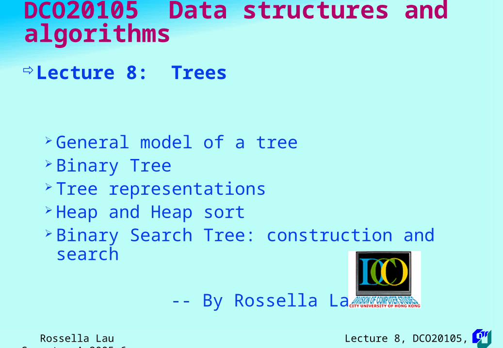
A tree in the above sense is called a free tree
By picking up a distinguished node, denoting it as a root, as the entrance of the tree, a tree can be represented as an oriented tree
A free tree may have numerous oriented trees corresponding to a given free tree
Rossella Lau Lecture 8, DCO20105, Semester A,2005-6
Different orientations of a tree
A
B D
C
EF
A
C D
E F
B
A
CD
E F
B
A
C BD
E F

Rossella Lau Lecture 8, DCO20105, Semester A,2005-6
Binary Tree
A binary tree can be empty or
partitioned into three disjointed subsets:
1. A single element called the root of the tree
2. A left sub-tree, which is a binary tree, of itself
3. A right sub-tree, which is a binary tree, of itself
Tree or binary tree’s definition is a recursive definition and operations on trees are usually in a recursive manner
Rossella Lau Lecture 8, DCO20105, Semester A,2005-6
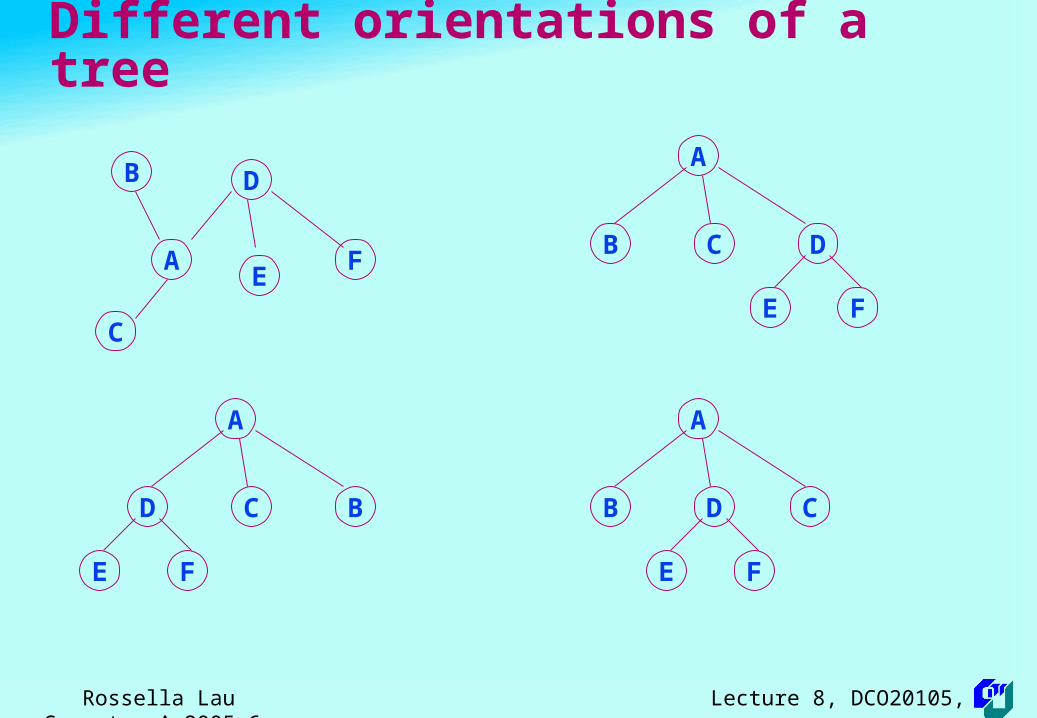
Notations of a binary tree
A
C
F
H I
B
D E
G
A is the root of the tree
A is the parent of B and C (B is the parent of D and E, …)
B is a left child of A
C is a right child of A
A or B is an ancestor of E
E or B is a descendant of A
B and C are siblings
D, G, H, I are leaves of the tree
The level of A is 0, the level of B is 1, …, the level of G is 3
Depth = max{ level of leaves} = 3

Rossella Lau Lecture 8, DCO20105, Semester A,2005-6
Structures that are not binary trees
A
C
F
I
B
D E
G H
All of these trees contain a tree which is not a sub-tree of itself
There is more than one path connecting two of the nodes
A
C
F
B
D E
G
A
C
F
B
D E
G
H I
Rossella Lau Lecture 8, DCO20105, Semester A,2005-6
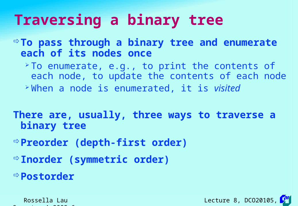
Traversing a binary treeTo pass through a binary tree and enumerate each of
its nodes once To enumerate, e.g., to print the contents of each node, to
update the contents of each node When a node is enumerated, it is visited
There are, usually, three ways to traverse a binary tree
Preorder (depth-first order)
Inorder (symmetric order)
Postorder
Rossella Lau Lecture 8, DCO20105, Semester A,2005-6
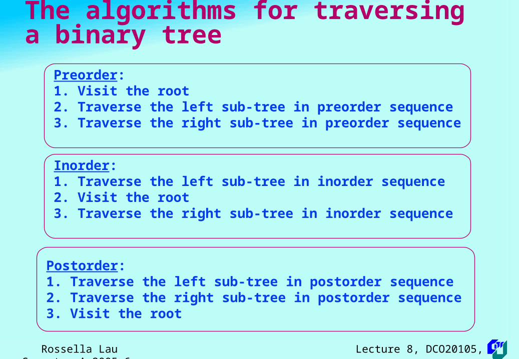
The algorithms for traversing a binary tree
Preorder:1. Visit the root2. Traverse the left sub-tree in preorder sequence3. Traverse the right sub-tree in preorder sequence
Inorder:1. Traverse the left sub-tree in inorder sequence2. Visit the root3. Traverse the right sub-tree in inorder sequence
Postorder:1. Traverse the left sub-tree in postorder sequence2. Traverse the right sub-tree in postorder sequence3. Visit the root

Rossella Lau Lecture 8, DCO20105, Semester A,2005-6
Examples of traversing a binary tree
For the binary tree on page 6
Preorder:
Inorder:
Postorder:

Rossella Lau Lecture 8, DCO20105, Semester A,2005-6
Representations of Binary Tree
Static: Vector representation
Dynamic: Pointer (Node) representation

Rossella Lau Lecture 8, DCO20105, Semester A,2005-6
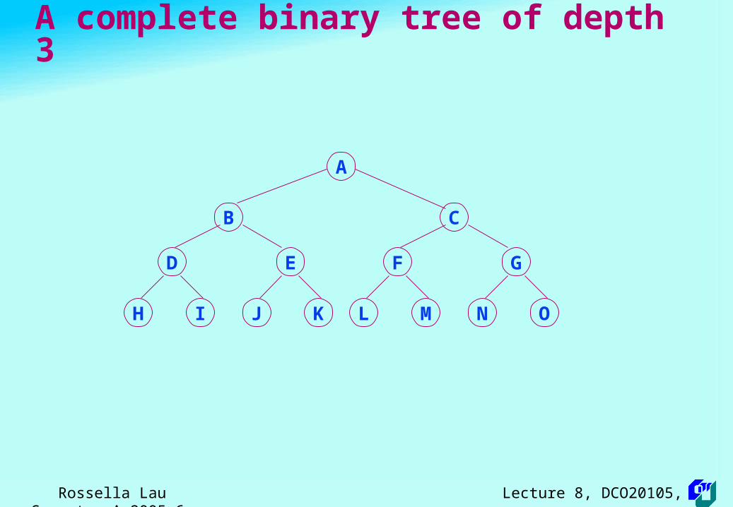
Complete binary treesA Complete binary tree of depth d:
all of whose leaves are at level d all of non-leaf (internal) nodes have exactly two children
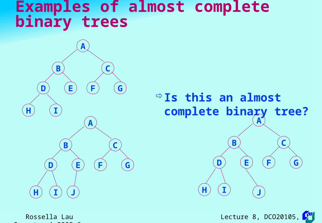
A binary tree of depth d is an almost complete binary tree if:
1. Any node n at level from 0 to d-2 has two children
2. For each node n in the tree with a right descendant at level d n must have a left child and every left descendant of n is either a leaf at level d or has
two children
Rossella Lau Lecture 8, DCO20105, Semester A,2005-6
A complete binary tree of depth 3
B
D E
A
H I J K
C
F G
L M N O
Rossella Lau Lecture 8, DCO20105, Semester A,2005-6
Examples of almost complete binary trees
B
D E
A
H I
C
F G
B
D E
A
H I
C
F G
J
Is this an almost complete binary tree?
B
D E
A
H I
C
F G
J
Rossella Lau Lecture 8, DCO20105, Semester A,2005-6
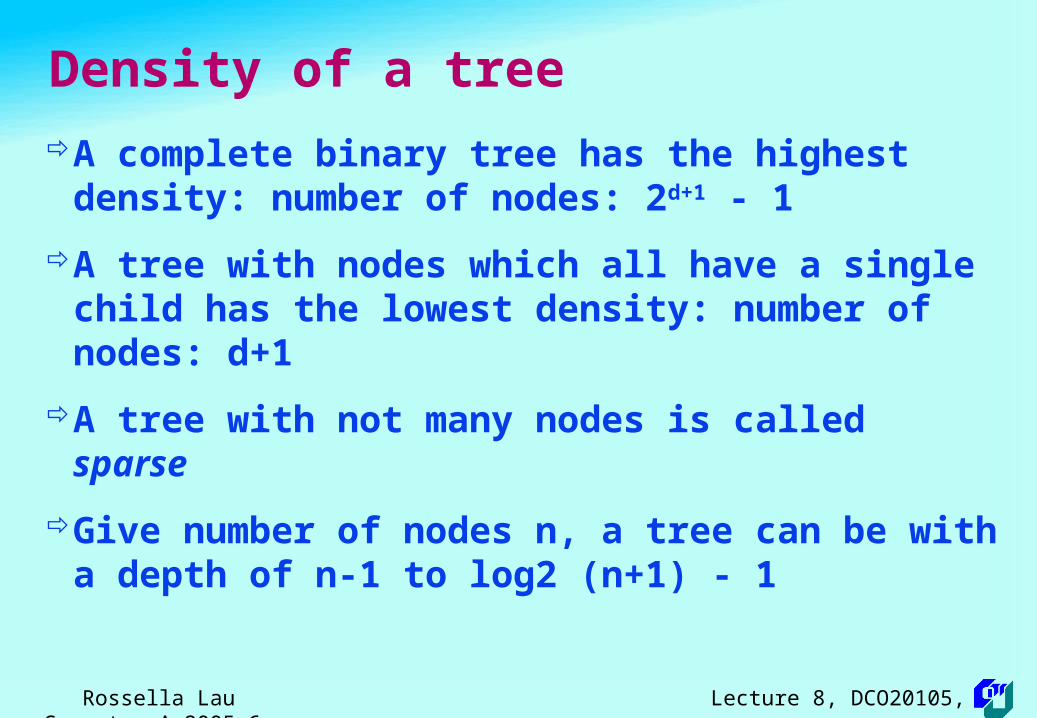
Density of a tree
A complete binary tree has the highest density: number of nodes: 2d+1 - 1
A tree with nodes which all have a single child has the lowest density: number of nodes: d+1
A tree with not many nodes is called sparse
Give number of nodes n, a tree can be with a depth of n-1 to log2 (n+1) - 1

Rossella Lau Lecture 8, DCO20105, Semester A,2005-6
Implicit array representation of a binary tree
For each almost complete binary tree, we can label each node from 0 to n, where n < (2d+1 - 1)
B
D E
A
H I
C
F G
J
0
1 2
3 4 5 6
7 8 9
The label is the subscript of an array The content of a numbered node can be stored in the corresponding position of an array
A B C D IE HF G J
0 1 2 3 84 75 6 9

Rossella Lau Lecture 8, DCO20105, Semester A,2005-6
Extensions to almost complete BT
B
A
C
D E
F G
I
H
J
K L
MB
A
C
D E
F G
I
H
J
K L
M
A B C D E
0 1 2 3 84 75 6 9
F G
1110 12
H I J K L M
0 1 2 3 84 75 6 9
For trees that are not a complete binary tree, we may add null nodes to make the trees become almost complete

Rossella Lau Lecture 8, DCO20105, Semester A,2005-6
Some operations on vector representationSome basic binary tree operations can be easily implemented:
vector<Data> bt; left_child(node): 2 * node + 1 right_child(node): 2 * (node + 1) parent(node): (node – 1) / 2 when node > 0 data(node): bt[node]
For efficient calculation of parent and children, representation may start the root from subscript at 1 instead of 0
left_child(node): 2 * node (equivalent to node<<1) right_child((node): left_child + 1 parent(node): node / 2 (equivalent to node>>1) the calculation can be simplified to bit-shift operations

Rossella Lau Lecture 8, DCO20105, Semester A,2005-6
Exercises on implicit representation
Ford’s written exercises: 14:11a, 12c
Rossella Lau Lecture 8, DCO20105, Semester A,2005-6
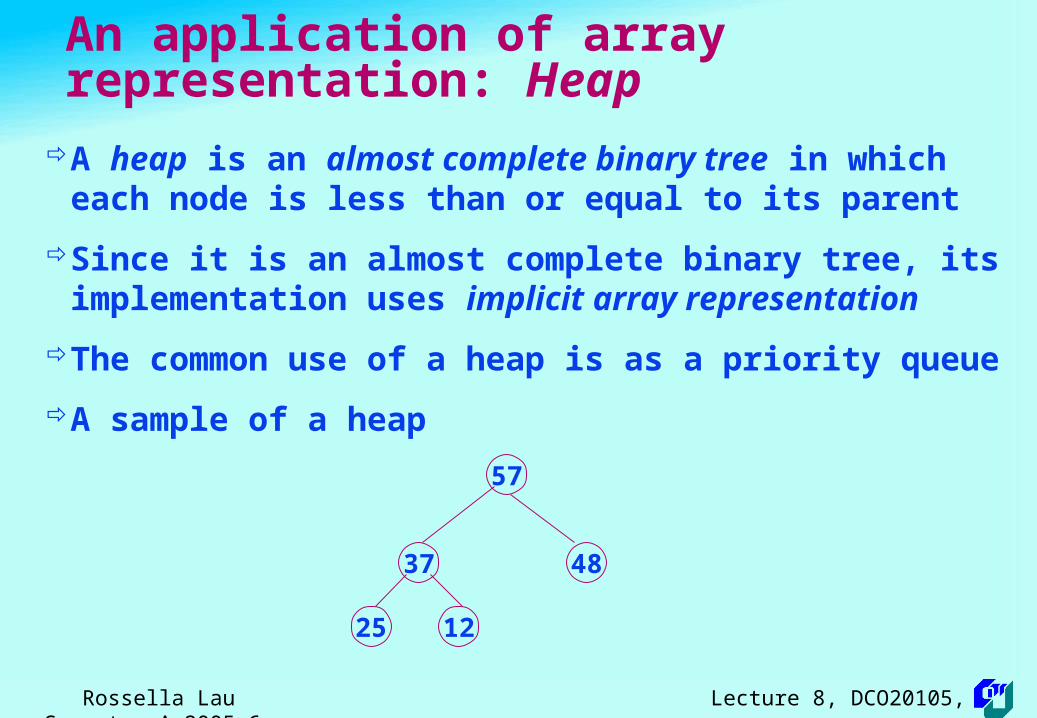
An application of array representation: Heap
A heap is an almost complete binary tree in which each node is less than or equal to its parent
Since it is an almost complete binary tree, its implementation uses implicit array representation
The common use of a heap is as a priority queue
A sample of a heap57
4837
25 12

Rossella Lau Lecture 8, DCO20105, Semester A,2005-6
Heap insert
To insert the item as the last leaf in the tree then shift it up whenever it is larger than its parent
E.g., Adding 92 to the previous heap
57
4837
25 12 92
57
4837
25 12 92
92
48
57
9237
25 12 48
92
57

Rossella Lau Lecture 8, DCO20105, Semester A,2005-6
Heap delete To remove the maximum from the heap:
1. Swap the root (maximum) with the last element in the array (the last node in the tree) the heap is reduced by one element
2. Shift the new root down whenever it is less than its larger child within the reduced heap
92
5767
25 12 22
22
5767
25 12 92
22
92
22
67
25
22
67
5725
22 12
Rossella Lau Lecture 8, DCO20105, Semester A,2005-6
Exercise on heap
Ford’s written exercises: 14:19b

Rossella Lau Lecture 8, DCO20105, Semester A,2005-6
Heap sortA binary tree can be represented by a vector; a list of
data in a vector can also be treated as an almost complete binary tree!
Heap sort makes use of this feature to construct data on a vector into a heap then sort data in order
It is a kind of selection sort Each time it finds the largest from a list (the heap) then
places it to the last position of the list The process continues the “selection” on the sub-lists
starting from the first elements which are not in the proper positions yet.

Rossella Lau Lecture 8, DCO20105, Semester A,2005-6
Heap sort method 1
1st phase: Construction of a heap it inserts elements to the heap one by one ()
2nd phase: Selection sort1. remove the maximum from the heap and replace it to
the last (the heap is reduced in the first n-1 nodes)
2. process continues until reduced heap becomes asingle node

Rossella Lau Lecture 8, DCO20105, Semester A,2005-6
An example of heap sort (method 1)
Input stream: 25 57 48 37 12 92 86 33
Then insert data one by one into the heap:
92
8637
33 12 48 57
25

Rossella Lau Lecture 8, DCO20105, Semester A,2005-6
Phase II of heap sort
86
5737
33 12 48 25
92
……
12
3325
37 48 57 86
92
92
8637
33 12 48 57
2592
2586
2557
25

Rossella Lau Lecture 8, DCO20105, Semester A,2005-6
Heapsort (method 2)
Instead of inserting data one by one, it converts the tree to a heap in the first phase makeHeap() in Ford: 14-2.
Iteratively applying the heap condition to each internal node (sub-trees) starting at the last and working up to the root
Then it applies the second phase of method 1

Rossella Lau Lecture 8, DCO20105, Semester A,2005-6
Phase I of method 2
25
4857
37 12 92 86
33
48
92 8637
33
92
4857
1237
25
57
92
25
25
86
48 86
25
37
33
12
9257
2592
8657
37 12 48 25
33

Rossella Lau Lecture 8, DCO20105, Semester A,2005-6
Performance of heap sort
For each insertion, it takes O(logn) because the process is on an almost complete binary tree
For n elements, it takes O(nlogn) even for worst case
Experiments show that heapsort doubles the time of quicksort but out performs quicksort in the worst case since the process keeps working on an almost complete binary tree (level at most log(n+1)).

Rossella Lau Lecture 8, DCO20105, Semester A,2005-6
Dynamic pointer representation
Reference program: BST.h: use two classes: BNode and BTree
template <class T>class BNode { T item; BNode *left; BNode *right; //end of data member ……}
template <class T>class BTree { BNode<T> *root; size_t countNodes; //end of data member ……}

Rossella Lau Lecture 8, DCO20105, Semester A,2005-6
Implementation of inorder traversal
template <classT>void BTree<T>::inOrder(BNode<T> const *bnode) const { if (bnode->left) inOrder(bnode->left);
cout << bnode->item << “ “;
if (bnode->right) inOrder(bnode->right); }
template<class T>void BTree<T>::inOrder() const { if ( root ) inOrder(root); else cout << “Empty tree\n”; }

Rossella Lau Lecture 8, DCO20105, Semester A,2005-6
Pretty tree In order to make a tree visible, we may imagine the tree with a
90 degree left rotation, then we have a special printing method: a reversed inorder traversal with nodes printed according to their levels
void prettyTree (BNode<T> const *bnode, size_t const level) const { if (bnode->right) prettyTree(bnode->right, level + 1);
// make space for different levels for (size_t i=0; i<level; i++) cout << “ “; cout << bnode->item << endl;
if (bnode->left) prettyTree(bnode->left, level + 1); }
void prettyTree () { if (root) pretty_tree(root, 0); else …… }

Rossella Lau Lecture 8, DCO20105, Semester A,2005-6
Binary Search Tree (BST)A BST is a binary tree in which all the key values stored
in the left descendents of a node are less than the key value of the node, and all the key values stored in the right descendants of a node are greater than the key value of the node. E.g.,
50
75
90
87 95
28
22 40
35

Rossella Lau Lecture 8, DCO20105, Semester A,2005-6
Dynamic representation for a BST
Same as a Binary Tree; sample program: BST.h
template <class T>class BSTNode { T item; BSTNode *left; BSTNode *right; //end of data member ……}
Template <class T>class BSTree { BSTNode<T> *root; size_t countNodes; //end of data member ……}

Rossella Lau Lecture 8, DCO20105, Semester A,2005-6
The algorithm for searching on a BSTThe searching can use a recursive approach.
BSTNode<T>* BSTree<T>::search (BSTNode const *node, T const& target) const { if ( target == node->item ) return node;
if ( target < node->item ) return node->left ? search(node->left, target) : 0; else return node->right? search(node->right, target): 0;}
BSTNode<T>* BSTree<T>::search (T const& target) const { return root ? search(root, target) : 0;}

Rossella Lau Lecture 8, DCO20105, Semester A,2005-6
The iterative version for searching on a BSTHowever, it is also quite easy to convert the recursive
algorithm to a non-recursive(iterative) one since it only involves "going down" the tree.
BSTNode<T>* BSTree<T>::search(T const& target) const { BSTNode<T> *cur = root; while (cur) { if (target == cur->item) return cur; if (target < cur->item;) cur = cur->left; else cur = crr->right; } return 0; }

Rossella Lau Lecture 8, DCO20105, Semester A,2005-6
A better way to return the result: find() Searching usually follows the operations of insert or delete but the traditional
search returns a null pointer when a new item is required to insert; i.e., the insert has to find the
proper position to insert the item, again! the node for deletion which requires checking if the node is on the right hand side
or the left hand side of its parent, again!
With the reference supported in C++, we can write a find() which is similar the one in List.h in Lecture 4 for efficient insert() and remove() with one single search operation even if these operations require a search to make sure the node does not exist or does exist
Node *& means a reference of pointer that can be interpreted as the reference of the location where the pointer stores. From another view, if the name is on the right hand side of an expression, it refers to the value of the pointer, i.e., the node pointed to by the pointer; if the name is on the left hand side, it refers to the location storing the pointer; or the "parent" of the node! Assigning new values to the name means to change its "child"!

Rossella Lau Lecture 8, DCO20105, Semester A,2005-6
The implementation of find()
BSTNode<T>*& find (T const & target) {
if ( !root || target == root->item ) return root;
BSTNode<T>* par = root; // parent of current node while( 1 ) { if ( target < par->item ) if (!par->left || target == par->left->item) return par->left; else par = par->left; else if (!par->right || target == par->right->item) return par->right; else par = par->right; }}

Rossella Lau Lecture 8, DCO20105, Semester A,2005-6
Insert an item with find()
To insert an item involves searching for the correct place and usually, a BST assumes no duplication, then attach the new node to the target found by find()
Add an additional function attach() to BSTree
bool attach( BSTNode<T> *& nodeRef, T const & x ){ nodeRef = new BSTNode<T>( x ); return nodeRef;}
bool insert(T const & target) { BSTNode<T> *& curRef ( find ( target ) ); if ( !curRef ) return attach(curRef, target); else return false; // duplication }

Rossella Lau Lecture 8, DCO20105, Semester A,2005-6
Construction of the BST using insert()Input sequence: 50, 28, 40, 75, 90, 22, 35, 95, 87
An online animation is also available at: http://www.cs.jhu.edu/~goodrich/dsa/trees/btree.html
87 9535
22
50
28
40
75
90

Rossella Lau Lecture 8, DCO20105, Semester A,2005-6
More exercises on BST
Ford’s exercises: 10:20, 22

Rossella Lau Lecture 8, DCO20105, Semester A,2005-6
Complexity considerationsIf the binary tree is constructed in a random order,
the levels of the left sub-tree and right sub-tree of the resulting tree may be similar and each later search process is similar to a binary search in an array
Therefore, the optimal complexity for searching on a BST is about O(log2n)
However, if the input sequence for the BST is in sequential order, it may result in the tree on the next page. The complexity of find() becomes O(n)
Therefore, the complexity of the search on a BST is from O(log2n) to O(n).

Rossella Lau Lecture 8, DCO20105, Semester A,2005-6
The worst case of searching on a BSTInput sequence: 22, 28, 35, 40, 50, 75, 87, 90, 95
28
22
35
40
50
75
87
90
95

Rossella Lau Lecture 8, DCO20105, Semester A,2005-6
Complexity for insert()
As the logic of insert() is find() + attach()
If there is a fast memory allocation method, the running time of attach() is O(1)
insert() is similar to find(), insert() has the same complexity as find()

Rossella Lau Lecture 8, DCO20105, Semester A,2005-6
SummaryA binary tree is a typical recursive structure and has three
parts: root, left and right sub-trees
A binary tree is used to being stored in node representation
Sometimes, it is also efficient to store a binary tree in implicit array (vector) representation and its typical applications are heap and heap sort which is quite an efficient sorting algorithm for all cases
There are three usual ways to traverse a binary tree: preorder, inorder, and postorder
The binary search tree (BST) keeps smaller values on the left side of a node and larger values on the right
The optimal complexity for insert/search of a BST is O(log2n)

Rossella Lau Lecture 8, DCO20105, Semester A,2005-6
ReferenceFord: 10.1-6, 14.1-2
Data Structures and Algorithms in C++ by Michael T. Goodrich, Roberto Tamassia, David M. Mount : Chapter 6,8
Example programs: BST.h, testBST.cpp
-- END --