Embed Size (px)
Citation preview
Linear Algebra Chapter 3: Linear systems and matrices Section 5: Gauss-Jordan elimination Page 1
Roberto’s Notes on Linear Algebra
Chapter 3: Linear systems and matrices Section 5
Gauss-Jordan elimination
What you need to know already: What you can learn here:
How to represent a linear system through a
matrix.
How to use elementary operations to solve a
system and how the correspond to elementary
row operations on a matrix.
The most efficient and effective way to solve a
linear system.
A method to manipulate matrices that will
lead to many useful and interesting
consequences.
I may have heard of Gauss before, but who was Jordan: his wife?
Not even close. Carl Frederick Gauss was a great German mathematician,
whose name is associated with practically every area of mathematics you will see.
Wilhelm Jordan was a German engineer (yes, one of those) who specialized in
geodesy (do you know what that is?). You’ll see the part they played in this method
after we start exploring how the method works.
Is that the method Gauss and Jordan used to eliminate each other? Just kidding! But is this the same elimination method we saw is Section 3.2?
No, and for two reasons: it works on the augmented matrix instead of the
system itself and it eliminates variables through a different sequence of steps than the
old method. And there are even additional advantages that you will appreciate in
later chapters.
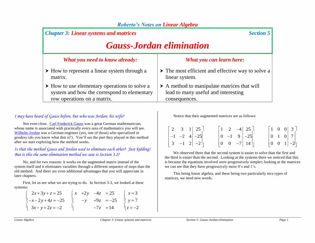
First, let us see what we are trying to do. In Section 3-3, we looked at these
systems:
2 3 25
2 4 25
3 2 2
x y z
x y z
x y z
2 4 25
9 25
7 14
x y z
y z
z
3
7
2
x
y
z
Notice that their augmented matrices are as follows:
2 3 1 25
1 2 4 25
3 1 2 2
1 2 4 25
0 1 9 25
0 0 7 14
1 0 0 3
0 1 0 7
0 0 1 2
We observed there that the second system is easier to solve than the first and
the third is easier than the second. Looking at the systems there we noticed that this
is because the equations involved were progressively simpler; looking at the matrices
we can see that they have progressively more 0’s and 1’s.
This being linear algebra, and these being two particularly nice types of
matrices, we need new words.
Linear Algebra Chapter 3: Linear systems and matrices Section 5: Gauss-Jordan elimination Page 2
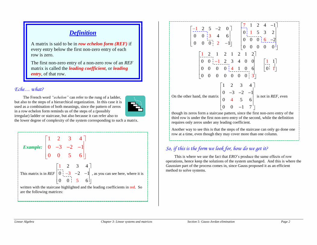
Definition
A matrix is said to be in row echelon form (REF) if
every entry below the first non-zero entry of each
row is zero.
The first non-zero entry of a non-zero row of an REF
matrix is called the leading coefficient, or leading
entry, of that row.
Eche… what?
The French word “echelon” can refer to the rung of a ladder,
but also to the steps of a hierarchical organization. In this case it is
used as a combination of both meanings, since the pattern of zeros
in a row echelon form reminds us of the steps of a (possibly
irregular) ladder or staircase, but also because it can refer also to
the lower degree of complexity of the system corresponding to such a matrix.
Example:
1 2 3 4
0 3 2 1
0 0 5 6
This matrix is in REF
2 3 4
0 2 1
0 0
1
6
3
5
, as you can see here, where it is
written with the staircase highlighted and the leading coefficients in red. So
are the following matrices:
2 5 2 0
0 0 4 6
0 0 0 1
1
3
2
1 2 4 1
0 5 3 2
0 0 0 2
0 0
1
6
0
7
0 0
2 1 2 1 2 1 2
0 0 2 3 4 0 0
0 0 0 0 1
1
1
4
3
0 6
0 0 0 0 0 0 0
1 1
0 1
On the other hand, the matrix
1 2 3 4
0 3 2 1
0 5 6
0 0 1 7
4
is not in REF, even
though its zeros form a staircase pattern, since the first non-zero entry of the
third row is under the first non-zero entry of the second, while the definition
requires only zeros under any leading coefficient.
Another way to see this is that the steps of the staircase can only go done one
row at a time, even though they may cover more than one column.
So, if this is the form we look for, how do we get it?
This is where we use the fact that ERO’s produce the same effects of row
operations, hence keep the solutions of the system unchanged. And this is where the
Gaussian part of the process comes in, since Gauss proposed it as an efficient
method to solve systems.
Linear Algebra Chapter 3: Linear systems and matrices Section 5: Gauss-Jordan elimination Page 3
Strategy to obtain an REF through
Gaussian elimination
In order to change an augmented matrix into an
equivalent REF:
1: If necessary, use a switch ERO to move a row
whose first entry is not zero to the top position of
the matrix.
2: If any of the rows below the first have a non-zero
entry in the first column, use suitable multiply and
add ERO’s to change such entries to 0.
3: Keeping the first row and the leading 0’s of the
remaining rows as they are, repeat the first two
steps on the smaller matrix consisting of the
remaining rows without the leading 0’s.
4: Repeat again the procedure until the REF is
achieved.
To keep the procedure simple when working by hand
on a matrix that consists of integers:
pick the desired ERO’s so as to avoid creating
fractions (unless you like working with fractions
), even if it means working bigger numbers;
use suitable ERO’s to change an existing leading
coefficient to 1, if this simplifies later steps and
does not create fractions.
Time out! This sounds awfully complicated!
Actually, this is a formal description of what we did in an earlier example,
where it worked fine. It turns out that it works every time! But you do have a point
in that this is a case of easier done than said, so let me give you a few pointers that
may clarify it and then I will show you some examples.
Knots on your finger
When using Gaussian elimination, it is useful to:
generate zeros in order, from the top down and
from the left to the right.
generate small integer numbers in the leading
entry positions. The number 1 is best, but not
necessary, especially if obtaining one means
creating fractions.
always use an upper row to change a lower row by
using an add ERO.
If all the entries of a row have a common factor,
eliminate it by using a multiply ERO, so that all
numbers become smaller.
Example:
2 3 25
2 4 25
3 2 2
x y z
x y z
x y z
To solve this system, we start from its augmented matrix:
2 3 1 25
1 2 4 25
3 1 2 2
We can then switch the first two rows and multiply the new row by -1, so as
to obtain a 1 in the leading position of the first row:
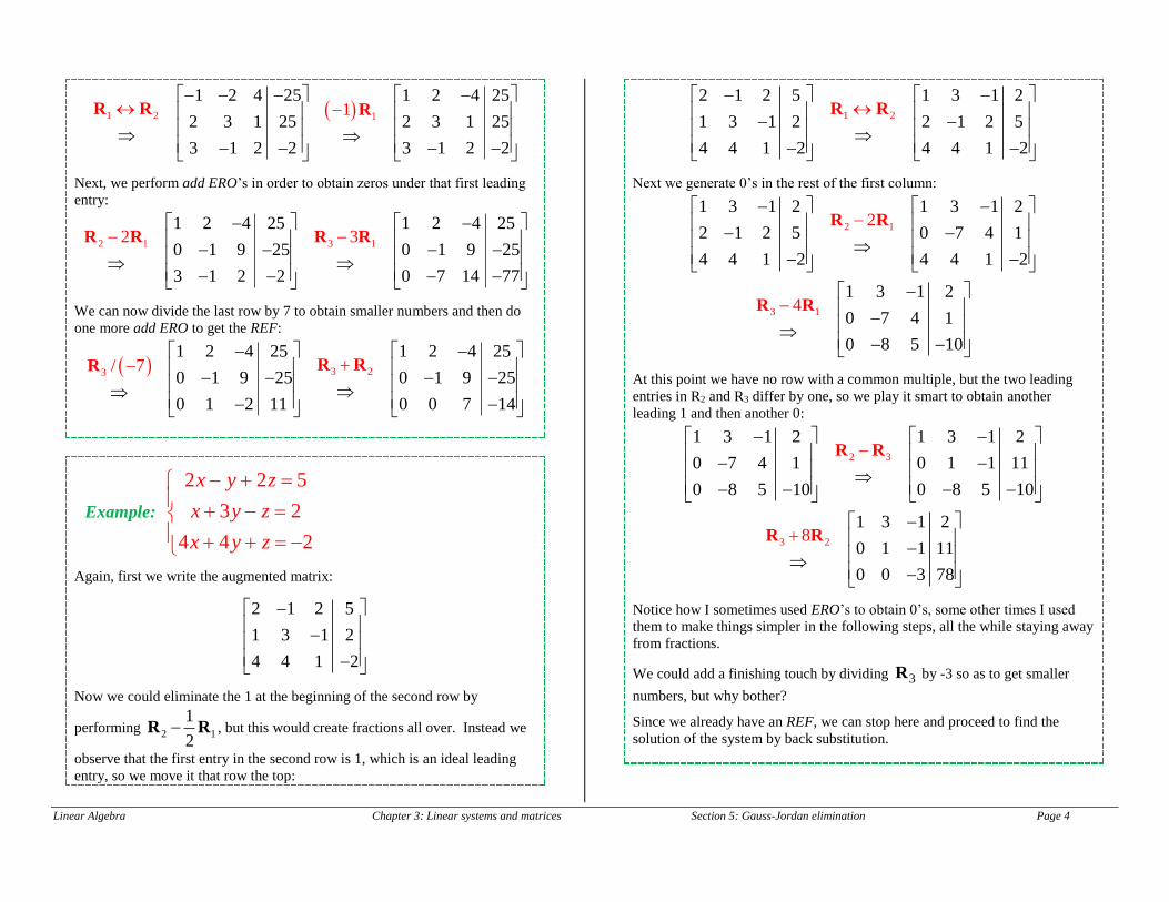
Linear Algebra Chapter 3: Linear systems and matrices Section 5: Gauss-Jordan elimination Page 4
1 2 1
1 2 4 25 1 2 4 25
2 3 1 25 2 3 1 25
3 1 2 2 3 1 2 2
1
R R R
Next, we perform add ERO’s in order to obtain zeros under that first leading
entry:
2 1 3 1
1 2 4 25 1 2 4 25
0 1 9 25 0 1 9 25
3 1 2 2 0
3
7 14
2
77
R R R R
We can now divide the last row by 7 to obtain smaller numbers and then do
one more add ERO to get the REF:
3 23
1 2 4 25 1 2 4 25
0 1 9 25 0 1 9 25
0 1 2 11 0 7 14
7
0
/
R RR
Example:
2 2 5
3 2
4 4 2
x y z
x y z
x y z
Again, first we write the augmented matrix:
2 1 2 5
1 3 1 2
4 4 1 2
Now we could eliminate the 1 at the beginning of the second row by
performing 2 1
1
2R R , but this would create fractions all over. Instead we
observe that the first entry in the second row is 1, which is an ideal leading
entry, so we move it that row the top:
1 2
2 1 2 5 1 3 1 2
1 3 1 2 2 1 2 5
4 4 1 2 4 4 1 2
R R
Next we generate 0’s in the rest of the first column:
2 121 3 1 2 1 3 1 2
2 1 2 5 0 7 4 1
4 4 1 2 4 4 1 2
R R
3 1
1 3 1 2
0 7 4 1
0 8 5 10
4
R R
At this point we have no row with a common multiple, but the two leading
entries in R2 and R3 differ by one, so we play it smart to obtain another
leading 1 and then another 0:
2 3
1 3 1 2 1 3 1 2
0 7 4 1 0 1 1 11
0 8 5 10 0 8 5 10
R R
3 2
1 3 1 2
0 1 1 11
0 0 3 78
8
R R
Notice how I sometimes used ERO’s to obtain 0’s, some other times I used
them to make things simpler in the following steps, all the while staying away
from fractions.
We could add a finishing touch by dividing 3R by -3 so as to get smaller
numbers, but why bother?
Since we already have an REF, we can stop here and proceed to find the
solution of the system by back substitution.
Linear Algebra Chapter 3: Linear systems and matrices Section 5: Gauss-Jordan elimination Page 5
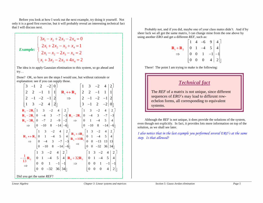
Before you look at how I work out the next example, try doing it yourself. Not
only it is a good first exercise, but it will probably reveal an interesting technical fact
that I will discuss next.
Example:
1 2 3 4
1 2 3 4
1 2 3 4
1 2 3 4
3 2 2 0
2 2 1
2 2 2
3 2 4 2
x x x x
x x x x
x x x x
x x x x
The idea is to apply Gaussian elimination to this system, so go ahead and
try…
Done? OK, so here are the steps I would use, but without rationale or
explanation: see if you can supply those.
1 4
3 1 2 2 0 1 3 2 4 2
2 2 1 1 1 2 2 1 1 1
2 1 2 1 2 2 1 2 1 2
1 3 2 4 2 3 1 2 2 0
R R
2 1
3 1 3 2
4 1
1 3 2 4 2 1 3 2 4 2
0 4 3 7 3 0 4 3 7 3
0 7 2 9 2 0 1 4
2
2 2
3 5 4
0 10 8 14 6 0 10 8 14 6
R R
R R R R
R R
3 2
2 3
4 2
1 3 2 4 2 1 3 2 4 2
0 1 4 5 4 0 1 4 5 4
0 4 3 7 3 0 0 13 13 13
0 10 8 14 6 0 0 32 36 3
4
0
4
1
R RR R
R R
4 33
1 3 2 4 2 1 3 2 4 2
0 1 4 5 4 0 1 4 5 4
0 0 1 1 1 0 0 1 1 1
0 0 32 36 3
132
2
13
4 0 0 0 4
R RR
Did you get the same REF?
Probably not, and if you did, maybe one of your class mates didn’t. And if by
sheer luck we all got the same matrix, I can change mine from the one above by
using another ERO and get a different REF, such as:
1 2
1 4 6 9 4
0 1 4 5 4
0 0 1 1 1
0 0 0 4 2
R R
There! The point I am trying to make is the following:
Technical fact
The REF of a matrix is not unique, since different
sequences of ERO’s may lead to different row-
echelon forms, all corresponding to equivalent
systems.
Although the REF is not unique, it does provide the solutions of the system,
even though not explicitly. In fact, it provides lots more information on top of the
solution, as we shall see later.
I also notice that in the last example you performed several ERO’s at the same step. Is that allowed?

Linear Algebra Chapter 3: Linear systems and matrices Section 5: Gauss-Jordan elimination Page 6
Technical fact
Several ERO’s may be performed at the same time,
provided that none of them would affect the result of
any of the others.
In particular, several add ERO’s may be performed at
the same time when they are all adding multiples of
the same row to the other rows.
This little innocent trick may add to the efficiency of the procedure, but make
sure to use it wisely and not to mix up operations that interfere with each other!
But we are still half way through, since we know that there is an even easier
form that we would like to get.
The one with 0’ above and the explicit solution!
Exactly! And 1’s as leading coefficients. Let’s give this form a name:
Definition
A matrix is said to be in reduced row echelon form
(RREF) if:
the leading coefficient of every non-zero row is 1
and
all entries above and below each leading
coefficient is zero.
I am not sure of why we need the leading entries to be all 1.
Because our goal now is to see the solution explicitly and having 1 as leading
entry means that the corresponding equation has the variable by itself, as needed for
an explicit solution. It will become clear through the examples, but first let us see
how to do it. The strategy is similar to Gaussian elimination to obtain an RREF, only
in reverse order.
Strategy to obtain the RREF through
Gauss-Jordan elimination
In order to change an REF matrix to its RREF:
1: Ignore any zero rows at the bottom of the matrix.
2: Use a multiply ERO to obtain 1 as leading entry in
the last non-zero row.
3: If the entry above the leading coefficient of the
last non-zero row is not 0, use suitable add ERO’s
to change it to 0.
4: Repeat steps 2 and 3 on progressively higher rows
and on all entries above leading coefficients until
the RREF is achieved.
Again, use suitable ERO’s to keep the numbers small
and integer if possible, although at this stage fractions
may become unavoidable.
So Jordan just extended the process so that we would get the simplest form.
Well, some explorers open the path; others make it smoother and more
comfortable! Let’s see how this works in our examples.
Linear Algebra Chapter 3: Linear systems and matrices Section 5: Gauss-Jordan elimination Page 7
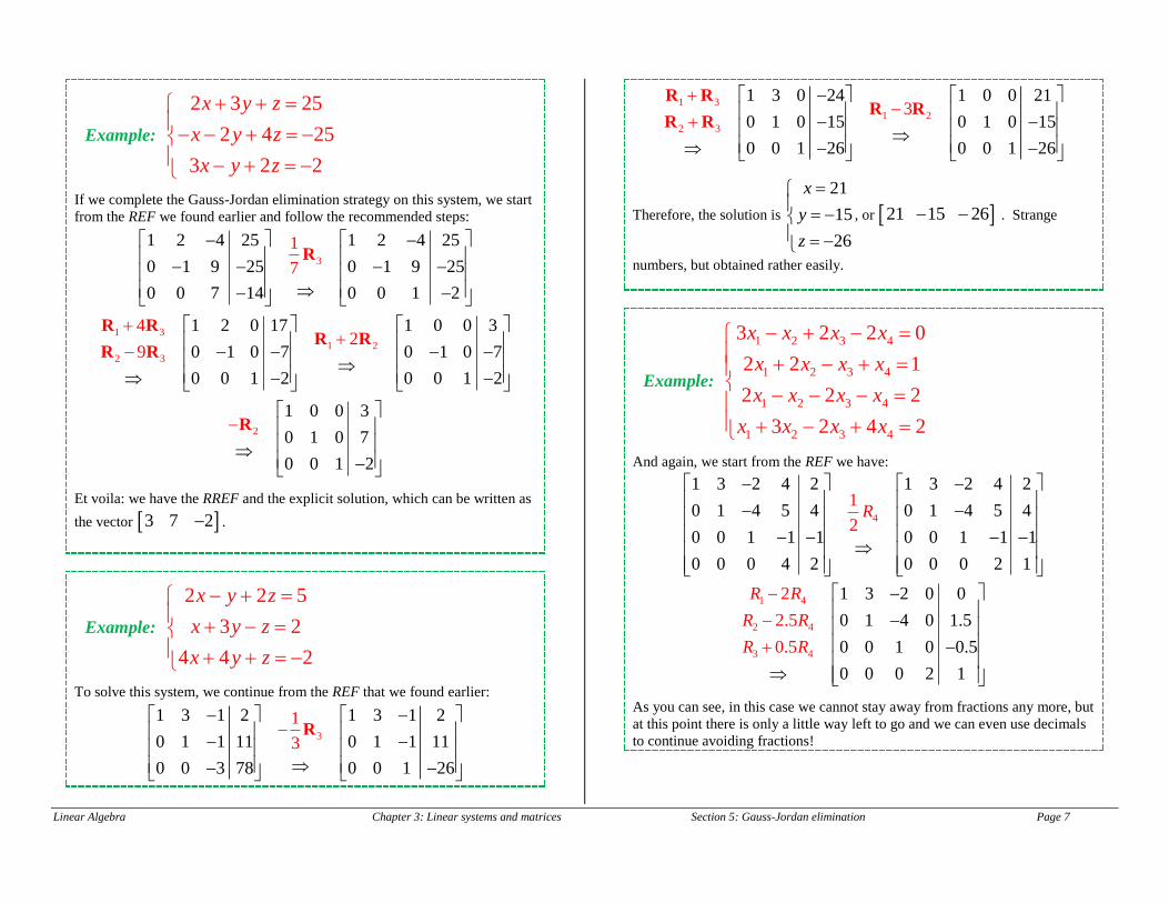
Example:
2 3 25
2 4 25
3 2 2
x y z
x y z
x y z
If we complete the Gauss-Jordan elimination strategy on this system, we start
from the REF we found earlier and follow the recommended steps:
3
1
7
1 2 4 25 1 2 4 25
0 1 9 25 0 1 9 25
0 0 7 14 0 0 1 2
R
1 3
1 2
2 3
1 2 0 17 1 0 0 3
0 1 0 7 0 1 0 7
0 0 1 2 0 0 1
4
9
2
2
R RR R
R R
2
1 0 0 3
0 1 0 7
0 0 1 2
R
Et voila: we have the RREF and the explicit solution, which can be written as
the vector 3 7 2 .
Example:
2 2 5
3 2
4 4 2
x y z
x y z
x y z
To solve this system, we continue from the REF that we found earlier:
3
1
3
1 3 1 2 1 3 1 2
0 1 1 11 0 1 1 11
0 0 3 78 0 0 1 26
R
1 3
1 2
2 3
1 3 0 24 1 0 0 21
0 1 0 15 0 1 0 15
0 0 1 26 0 0 1 26
3
R RR R
R R
Therefore, the solution is
21
15
26
x
y
z
, or 21 15 26 . Strange
numbers, but obtained rather easily.
Example:
1 2 3 4
1 2 3 4
1 2 3 4
1 2 3 4
3 2 2 0
2 2 1
2 2 2
3 2 4 2
x x x x
x x x x
x x x x
x x x x
And again, we start from the REF we have:
4
1 3 2 4 2 1 3 2 4 2
0 1 4 5 4 0 1 4 5 4
0 0 1 1 1 0 0 1 1 1
0 0 0 4 2 0 0
1
2
0 2 1
R
1 4
2 4
3 4
1 3 2 0 0
0 1 4 0 1.5
0 0 1 0 0.5
0 0 0
2
2.5
0.
2 1
5
R R
R R
R R
As you can see, in this case we cannot stay away from fractions any more, but
at this point there is only a little way left to go and we can even use decimals
to continue avoiding fractions!
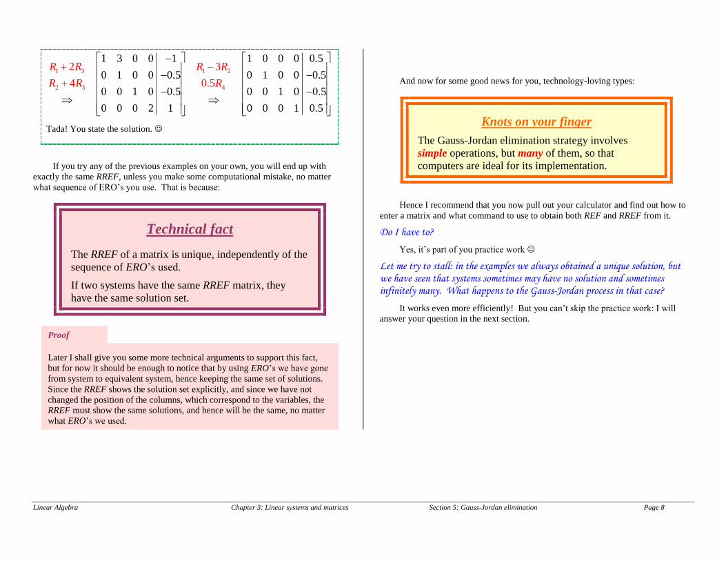
Linear Algebra Chapter 3: Linear systems and matrices Section 5: Gauss-Jordan elimination Page 8
1 3 1 2
2 3 4
1 3 0 0 1 1 0 0 0 0.5
0 1 0 0 0.5 0 1 0 0 0.5
0 0 1 0 0.5
2 3
0 0 1 0 0.5
0 0 0 2 1
4 0.5
0 0 0 1 0.5
R R R R
R R R
Tada! You state the solution.
If you try any of the previous examples on your own, you will end up with
exactly the same RREF, unless you make some computational mistake, no matter
what sequence of ERO’s you use. That is because:
Technical fact
The RREF of a matrix is unique, independently of the
sequence of ERO’s used.
If two systems have the same RREF matrix, they
have the same solution set.
Proof
Later I shall give you some more technical arguments to support this fact,
but for now it should be enough to notice that by using ERO’s we have gone
from system to equivalent system, hence keeping the same set of solutions.
Since the RREF shows the solution set explicitly, and since we have not
changed the position of the columns, which correspond to the variables, the
RREF must show the same solutions, and hence will be the same, no matter
what ERO’s we used.
And now for some good news for you, technology-loving types:
Knots on your finger
The Gauss-Jordan elimination strategy involves
simple operations, but many of them, so that
computers are ideal for its implementation.
Hence I recommend that you now pull out your calculator and find out how to
enter a matrix and what command to use to obtain both REF and RREF from it.
Do I have to?
Yes, it’s part of you practice work
Let me try to stall: in the examples we always obtained a unique solution, but we have seen that systems sometimes may have no solution and sometimes infinitely many. What happens to the Gauss-Jordan process in that case?
It works even more efficiently! But you can’t skip the practice work: I will
answer your question in the next section.

Linear Algebra Chapter 3: Linear systems and matrices Section 5: Gauss-Jordan elimination Page 9
Summary
By using ERO’s in a well-managed way, we can solve any linear system through a fast, simple and programmable procedure.
The idea of variable elimination leads to the REF of a matrix (and its system), while following it with back substitution leads to the RREF.
Common errors to avoid
The Gauss-Jordan elimination procedure is like chess: it is easy to understand the individual moves, but it takes practice to combine them into a winning game, that is, a truly
easy and fast method to obtain the solution of a system in every case.
Watch out for the “silly” errors that can occur as a result of the large number of easy computations it requires.
Remember that any matrix has infinitely many REF’s, but only one RREF. If you get a different RREF, someone has made a mistake, and it may be you!
Learning questions for Section LA 3-5
Review questions:
1. Describe how the Gauss-Jordan elimination method works.
2. Compare and contrast Gaussian elimination and Gauss-Jordan elimination.
3. Explain what the REF and the RREF of a matrix and of a system are.
4. Clarify the difference between the required steps of the Gauss-Jordan
elimination procedure and the optional ones to use when performing it by hand.
Memory questions:
1. What form of a matrix is obtained as the result of Gaussian elimination?
2. What form of a matrix is obtained as the result of Gauss-Jordan elimination?
3. How many REF’s does a matrix have?
4. How many RREF’s does a matrix have?
Linear Algebra Chapter 3: Linear systems and matrices Section 5: Gauss-Jordan elimination Page 10
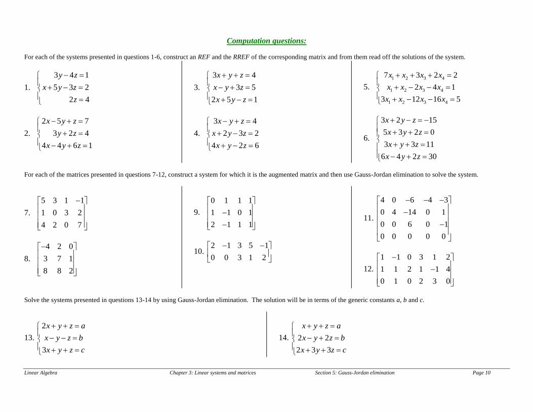
Computation questions:
For each of the systems presented in questions 1-6, construct an REF and the RREF of the corresponding matrix and from them read off the solutions of the system.
1.
3 4 1
5 3 2
2 4
y z
x y z
z
2.
2 5 7
3 2 4
4 4 6 1
x y z
y z
x y z
3.
3 4
3 5
2 5 1
x y z
x y z
x y z
4.
3 4
2 3 2
4 2 6
x y z
x y z
x y z
5.
1 2 3 4
1 2 3 4
1 2 3 4
7 3 2 2
2 4 1
3 12 16 5
x x x x
x x x x
x x x x
6.
3 2 15
5 3 2 0
3 3 11
6 4 2 30
x y z
x y z
x y z
x y z
For each of the matrices presented in questions 7-12, construct a system for which it is the augmented matrix and then use Gauss-Jordan elimination to solve the system.
7.
5 3 1 1
1 0 3 2
4 2 0 7
8.
4 2 0
3 7 1
8 8 2
9.
0 1 1 1
1 1 0 1
2 1 1 1
10. 2 1 3 5 1
0 0 3 1 2
11.
4 0 6 4 3
0 4 14 0 1
0 0 6 0 1
0 0 0 0 0
12.
1 1 0 3 1 2
1 1 2 1 1 4
0 1 0 2 3 0
Solve the systems presented in questions 13-14 by using Gauss-Jordan elimination. The solution will be in terms of the generic constants a, b and c.
13.
2
3
x y z a
x y z b
x y z c
14. 2 2
2 3 3
x y z a
x y z b
x y z c
Linear Algebra Chapter 3: Linear systems and matrices Section 5: Gauss-Jordan elimination Page 11
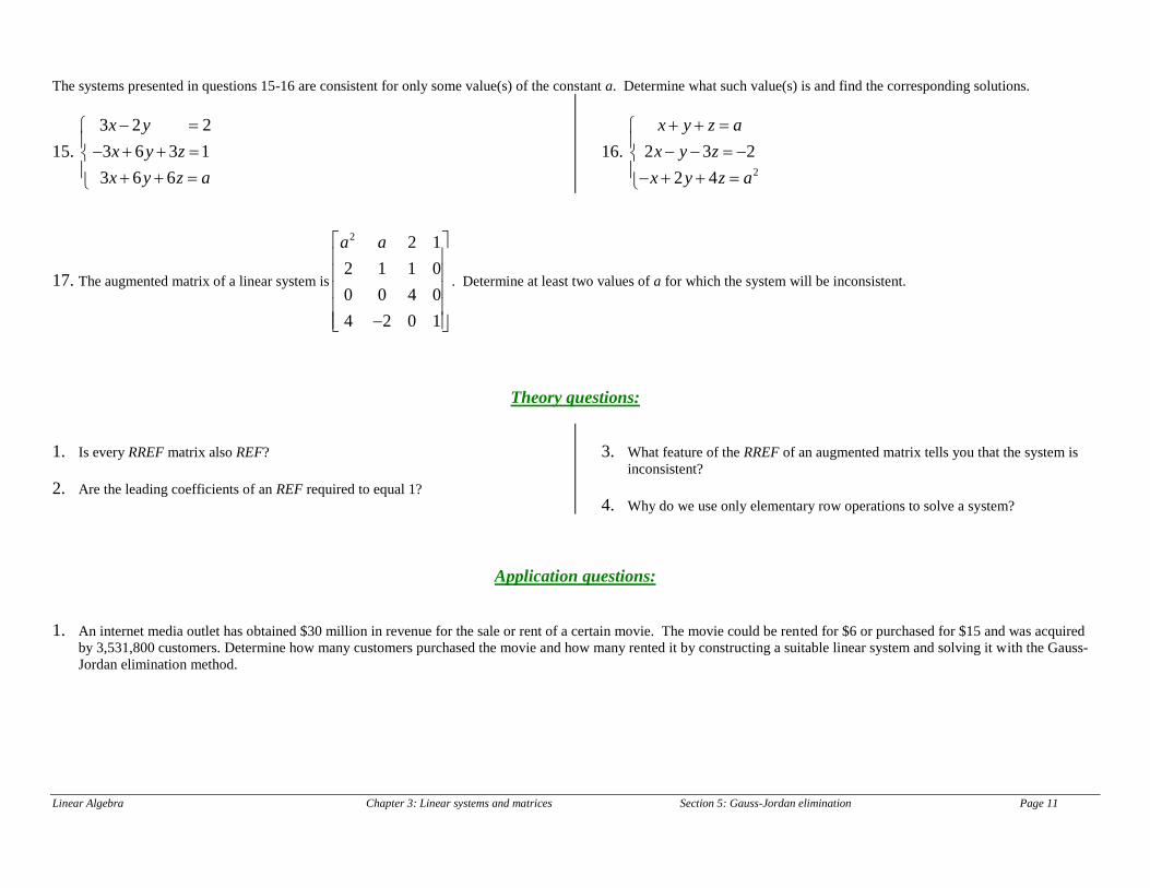
The systems presented in questions 15-16 are consistent for only some value(s) of the constant a. Determine what such value(s) is and find the corresponding solutions.
15.
3 2 2
3 6 3 1
3 6 6
x y
x y z
x y z a
16. 2
2 3 2
2 4
x y z a
x y z
x y z a
17. The augmented matrix of a linear system is
2 2 1
2 1 1 0
0 0 4 0
4 2 0 1
a a
. Determine at least two values of a for which the system will be inconsistent.
Theory questions:
1. Is every RREF matrix also REF?
2. Are the leading coefficients of an REF required to equal 1?
3. What feature of the RREF of an augmented matrix tells you that the system is
inconsistent?
4. Why do we use only elementary row operations to solve a system?
Application questions:
1. An internet media outlet has obtained $30 million in revenue for the sale or rent of a certain movie. The movie could be rented for $6 or purchased for $15 and was acquired
by 3,531,800 customers. Determine how many customers purchased the movie and how many rented it by constructing a suitable linear system and solving it with the Gauss-
Jordan elimination method.

Linear Algebra Chapter 3: Linear systems and matrices Section 5: Gauss-Jordan elimination Page 12
Templated questions:
1. Whenever using the Gauss-Jordan elimination method, identify where the Gaussian process ends and the “Jordan” phase begins.
What questions do you have for your instructor?