Equitable Handicapping in GolfDerek R. Bingham and Tim B. Swartz �AbstractPrevious studies on handicapping have suggested that in matches between 2 golfers, the better golferhas an advantage. In this paper, we consider medal play between 2 golfers when they are both playingwell. The study uses the new slope system for handicapping. In this context we argue that it is actuallythe weaker golfer who has an advantage. The conclusions are based on both the analysis of actual golfscores and the analysis of theoretical models. We suggest an alternative scoring formula which leads to\fairer" competitions.Keywords : data analysis, statistical modelling, order statistics.�D. Bingham is Assistant Professor, Department of Statistics, University of Michigan, Ann Arbor MI, 48109. T. Swartzis Associate Professor, Department of Mathematics and Statistics, Simon Fraser University, Burnaby BC, Canada V5A1S6.T. Swartz was partially supported by a grant from the Natural Sciences and Engineering Research Council of Canada. Theauthors thank the Pemberton Golf and Country Club, Pemberton, British Columbia for access to their golf records. Theauthors also thank the editor and the associate editor for helpful comments that lead to an improvement in the manuscript.1

1. INTRODUCTIONThe purpose of handicapping in the game of golf is to allow golfers of varying skill levels to competefairly. The fairness of handicap systems has been addressed by a number of authors. For instance, Tallis(1994) investigated handicapping in various team competitions and found that certain handicap systemscan be extremely unfair. In this paper, we focus on matches between 2 golfers. In such matches, thegeneral consensus is that handicap systems tend to favour the better golfer. For example, Scheid (1977)looked at 1000 scores obtained from members of the Plymouth Country Club in Plymouth, Massachusetts.Using simulated matches based on these scores, he calculated the winning proportion for the better golferin medal play using handicaps. He found that with handicap di�erentials greater than 3, the winningproportion for the better golfer exceeded 60% and was as high as 85%. Pollock (1977) used a theoreticalgolf model based on the normal distribution and found that under reasonable variance assumptions, thebetter golfer has a competitive advantage in both medal play and match play. In a nice overview of thestatistical literature pertaining to golf, Larkey (1998) explains that the pioneering work of Francis Scheid,beginning with Scheid (1971) was instrumental in initiating changes to the handicap system.We address a slightly di�erent problem in the context of medal play using the current handicap system.We are not concerned with the probability that golfer A defeats golfer B where golfer A is the better golfer.Rather, we are interested in the conditional probability that golfer A defeats golfer B when they are bothplaying well. Under a fair handicap system, the conditional probability that golfer A defeats golfer Bshould be .5. From a tournament perspective, this is a most practical issue. For a golfer does not expectto win a prize when he plays poorly, but when he plays well, at the very least, he expects a fair chance of2

winning a prize.The central idea of this paper is that golfers with higher handicaps (i.e. weaker golfers) tend to havemore variability in their golf scores. Consequently, the weaker golfer is more likely to post results wellbelow (or above) their typical scores. Under the current handicap system (i.e. the slope system), thisgreater variability is not taken into consideration. We demonstrate that this gives an advantage to theweaker golfer when both golfers play well.In Section 2, we brie y describe handicapping and indicate changes that have taken place in thehandicap system since the papers of Scheid (1977) and Pollock (1977). Some real data are analyzed inSection 3. We see that in medal play using handicaps, the opposite e�ect to that observed in Scheid(1977) and Pollock (1977) takes place. That is, when both golfers are playing well, it is actually theweaker golfer who has an advantage in winning a match. The advantage is most dramatic when the bettergolfer happens to be a low-handicapper. In Section 4, we observe the same phenomenon by approachingthe problem from a theoretical perspective. In Section 5, we describe a simple alternative scoring formulafor use in tournament play and suggest that it is a more equitable method for prize distribution. We thenconclude with some caveats and closing remarks.2. HANDICAPPING IN GOLFSince the publication of the articles by Scheid (1977) and Pollock (1977), there have been changes tothe United States Golf Association (USGA) handicap system. Consider a golfer who has completed atleast 20 rounds of golf and wishes to update his handicap. We refer to a gross score as a golfer's actualscore obtained by summing his strokes over 18 holes. Using the old handicap system, a di�erential DOld3

is de�ned as DOld = X �Rwhere X is the adjusted gross score modi�ed according to equitable stroke control (see Table 1) and Ris the course rating for the course being played. Using the old handicap system, the golfer's handicapis calculated by averaging the 10 lowest di�erentials in the last 20 rounds, multiplying by .96 and thenrounding to the nearest integer value. When playing on any course, a golfer's net score in medal playis then obtained by subtracting his handicap from his gross score. We note that only a golfer's lowestdi�erentials (i.e. best rounds) are used in the handicap calculation. This is because the best roundsprovide a better indication of ability; when a golfer is playing poorly, it is easy to lose concentration andhave scores deteriorate. Using only the lowest di�erentials also provides a deterrent to the \sandbagger"who arti�cially attempts to in ate his handicap by intentionally playing poorly.Since the early 1990's, the slope system has been gradually introduced to golf courses across NorthAmerica as an enhancement to fair handicapping. The slope system generalizes the old handicap systemby further considering course di�culty. Consider then a golfer who has completed at least 20 roundswhere none of the resultant scores are deemed to be \eligible tournament" scores. The de�nition of thedi�erential D is modi�ed from DOld = X � R toD = 113(X �R)S4

where S is the slope rating for the course. A handicap index I is then obtained by averaging the 10 lowestdi�erentials in the most recent 20 rounds, multiplying by .96 and truncating to 1 decimal place. Whenplaying on a given course with slope rating S�, the number of handicap strokes is now determined to beI(S�=113) rounded to the nearest integer value. If the competition is net medal play between 2 golfers,then the golfer's net score is obtained by subtracting the handicap strokes from his gross score. At thispoint we emphasize the distinction between the handicap index I and the number of handicap strokes fora given match; this distinction is important throughout the remainder of the paper.In Table 2, we provide an example of the calculation of di�erentials under both handicap systems.Using the old system, the golfer receives :96(158:3=10)! 15 handicap strokes independent of the courseand the set of tees. Using the slope system, the golfer has a handicap index of :96(154:8=10)! 14:8, and,for example, is allotted 14:8(120)=113! 16 handicap strokes when playing from a set of tees on a coursewhose slope rating is 120.Consider then 2 golfers who play most of their rounds on courses of average di�culty (i.e. S � 113)and then play an easy course (i.e. S� < 113). From the de�nitions above, it is clear that they receiveproportionally fewer handicap strokes under the slope system than under the old system. Similarly, theyreceive proportionally more handicap strokes under the slope system than under the old system whenplaying a di�cult course (i.e. S� > 113). If we accept the results of the existing literature that suggestthat the better golfer always has an advantage, then it follows that the advantage on an easy course willbe even more pronounced under the slope system.For detailed information on the calculation of handicaps, eligible tournament scores, equitable stroke5

control, etc., see the USGA handicap web page at www.usga.org/handicap/manual. For information onthe theory underlying the slope system, see Scheid (1995) and the references therein.3. DATA ANALYSISData were collected from the computer handicap system at the Pemberton Valley Golf and CountryClub in Pemberton Valley, British Columbia during the 1997 golf season. Only full data on rounds playedat Pemberton Valley were available. From the white tees, Pemberton Valley is a 5972 yard golf coursewith a course rating of 68.5 and a slope rating of 120. From the blue tees, Pemberton Valley measures6407 yards with a course rating of 70.5 and a slope rating of 124. We demonstrate that in a competitionbetween 2 golfers, the better golfer is disadvantaged in medal play when both golfers are playing well.In this section, all reference to net scores should actually be interpreted as adjusted net scores wheretwo adjustments are made. The �rst adjustment is due to equitable stroke control. Unfortunately, mem-bers enter adjusted gross scores into the computer database and there is no method of retrieving the(unadjusted) gross scores. However, we do not anticipate this to be a problem as we consider only thevery best rounds of golf. Presumably, when a golfer is playing very well, the adjusted gross score will beequal or nearly equal to the gross score. The second adjustment is a standardization that transforms anadjusted gross score X1 on a course with course rating R1 and slope rating S1 to an adjusted gross scoreR2+S2(X1�R1)=S1 corresponding to a course with course rating R2 and slope rating S2. The standard-ization is based on the recognition that the di�erential 113(X1 � R1)=S1 is equivalent to the di�erential113(X2 � R2)=S2. In our analysis, we transform scores from the blues tees to scores from the white teesat Pemberton Valley. 6

We limit our analysis to the 49 male members who completed 40 or more rounds during the year. Weuse the �rst 20 rounds as a tuneup period to allow the golfer to reach \mid-season" form and to allowthe handicap index to settle. We also restrict our study to the immediate 20 rounds following the tuneupperiod. We hope that by using a shortened period, golfers will not experience dramatic changes in theirskill levels. Each golfer will also have completed the same number of rounds of golf. Therefore our dataanalysis is based on 49(20) = 980 scores.For each of the 49 golfers, we calculate net scores for each of the 20 rounds subsequent to the initial 20rounds of golf. We then take each golfer's best net score and use this as a measure of when the golfer isplaying well. In Figure 1, we plot the minimum net score versus the handicap index I where the handicapindex is calculated immediately after the tuneup period. We see that the plot has a negative regressionline (slope = -.10) indicating that the weaker golfer has a better chance of defeating the stronger golferwhen they both play well. A statistical test for the slope gives a marginally signi�cant p-value of :049,where of course it is more di�cult to establish an e�ect when the e�ect size is small. To put the plot intoperspective, we would expect a 25-handicapper to beat a 5-handicapper by (25�5)(:10) = 2 net strokes inmedal play when they are both playing their best games. This highlights the considerable inequity facingthe low-handicapper in tournaments where only a few players win prizes.Using the same data set, we again consider the 49 golfers and choose their best m net scores amongstthe 20 rounds immediately following the initial tuneup period. Again, the net scores are based on thehandicap index I determined at the end of the tuneup period. With m scores for each golfer, there are�492 �m2 possible matches between 2 golfers that can be simulated. The matches are simulated in the7

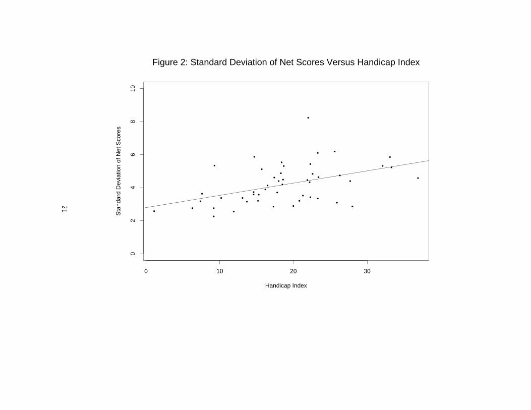
sense that the 2 golfers have not directly competed against one another. We consider m = 2; 3; 4 as thisrepresents the best 10%, 15% and 20% of net scores (i.e. occasions when the golfers play well). We excludefrom the analysis the 5 pairs of golfers that have the same handicap index. In Table 3, we give the resultsof the simulated matches, and again, we observe that the weaker golfer enjoys an advantage when bothgolfers are playing well. For example, with m = 2, the weaker golfer wins or ties 65:6% of the matches.In Figure 2, we plot the sample standard deviation of the 20 net scores following the tuneup periodversus the handicap index established at the end of the tuneup period. The least squares line has a slope of.07 and a corresponding p-value of :001. In this plot we see that the low handicap golfer is generally moreconsistent than the high handicap golfer. This result is not surprising. However, it does have implicationsfor the fairness of matches when both golfers are playing well. This result, together with Figure 1, suggeststhat the very low handicap golfer has little chance of winning a tournament based on net scores.We remark that these results are striking and contradict the USGA literature. From section 10-2 of theUSGA Handicap Formula manual on the USGA web page, we quote, \As your Handicap Index improves(gets lower), you have a slightly better chance of placing high or winning a handicap event".4. ANALYSIS OF A NORMAL MODELThe use of the normal distribution in modelling golf scores has been previously considered in theliterature. For example, Pollock (1977) used a normal model to investigate theoretical properties of hand-icapping. More notably, Scheid (1990) carried out an extensive analysis on the distribution of golf scores.Except for a slightly longer right tail, Scheid (1990) found the normal approximation to be satisfactory.8

In this analysis, we de�ne Xij as the gross score corresponding to the i-th golfer on the j-th coursewith course rating Rj and slope rating Sj . We assume that scores are independent and thatDij = 113(Xij � Rj)Sj � Normal[�i; �2i ]: (1)The normality assumption can be motivated by the Central Limit Theorem by noting that gross scoresare obtained by summing the number of strokes taken over 18 holes. The assumption of the constancy ofthe distribution of Dij over courses and tees is essentially the rationale for the slope system. Note thatDij is not quite a di�erential since Xij has not been modi�ed according to equitable stroke control.To test the adequacy of model (1), we calculate the Cram�er-von Mises statisticW 2 and the correspond-ing p-value (page 122 of D'Agostino and Stephens, 1986) for each of the 49 golfers using the di�erentialsobtained over the 20 post tuneup rounds. The results are consistent with the hypothesis of normality asonly 2 of the 49 p-values (.046 and .047) are signi�cant at level .05. When using the Anderson-Darlingstatistic A2, only 1 p-value (.039) is found to be signi�cant. With respect to the Scheid (1990) study, weobserve that the slight departures from normality appear to be the result of a shorter than expected lefttail. Although we recognize de�ciencies in the model such as the approximation of a discrete distribu-tion by a continuous distribution, the model provides insight on a number of handicap issues as well asmotivation for a new scoring formula as developed in Section 5.Now according to model (1), consider two golfers playing the same course so that we can drop thesubscript j. Let Hi be the number of handicap strokes for the i-th golfer as described in Section 2, and9

without loss of generality let H1 < H2 such that the �rst golfer is the better player. ThenXi � Normal[�i; �2i ]where ui = R+ S�i=113 and �i = S�i=113. Our interest lies in the investigation ofPk = Prob(the better golfer wins j both golfers play well)= Prob(X1 �H1 < X2 �H2 j Xi < �i � k�i; i = 1; 2)where k > 0. Here, Xi �Hi represents the net score of golfer i and we condition on both golfers playingbetter than k standard deviations below their average gross score. Since �i � Hi represents the averagenet score of golfer i, it follows from the results of Scheid (1977) and Pollock (1977) that� = (�2 �H2)� (�1 �H1) > 0:When �1 < �2 and k > �=(�2 � �1), it is then easily shown thatPk = R ��k�2�1z=�1 �(z) h�(�k)� � ��1z���2 �i dz�2(�k)where � is the density and � is the cumulative distribution function of the standard normal. To get asense of Pk for realistic values of k, consider typical values � = 1, �1 = 2 and �2 = 3. Integrating viaSimpson's rule, we obtain the decreasing probabilities P1:0 = :39, P1:5 = :22, P2:0 = :10 and P2:5 = :03.10

Now let G(z) be such that G0(z) = �(z) h�(�k)� � ��1z���2 �i and G(�1) = 0. Thenlimk!1 Pk = limk!1 G ���k�2�1 ��2(�k) = 0where the second equality follows from an application of l'Hospital's rule. Therefore, as both golfers playbetter (i.e. k ! 1), it becomes impossible for the better golfer to win the match. This conclusion is inthe same direction as the empirical results from Section 3.Mosteller and Youtz (1992) considered the scores of professional golfers during the �nal 2 roundsof PGA tournaments under ideal weather conditions. They found that adjusted scores could be wellapproximated by a base score plus a Poisson variate. Whereas the Mosteller and Youtz (1992) analysisinvolved the most homogeneous of conditions, we are faced with data involving golfers of varying skilllevels playing under various conditions. Furthermore, little is at stake for our golfers and we therefore donot expect their e�ort to be constant over all rounds. In an earlier version of this paper (which is availableupon request), we extend the Mosteller and Youtz (1992) model such that the net score of the i-th golferXi �Hi is given by Xi �Hi = Bi +Wiwhere Bi is the idealized or perfect base score for the i-th golfer and Wi � Poisson(�i). This model leadsto the same theoretical result that the better golfer is disadvantaged when two golfers play well.11

5. AN ALTERNATIVE TO NET SCORESIn this section we propose a simple method for promoting fairness in matches. It is based on thenormal model from Section 4 and consideration of the slope system. From model (1), it follows thatT = Dij � �i�ihas the same distribution (i.e. standard normal) for all golfers and ought to be a \fairer" yardstick thanusing the traditional net score. Moreover, T ought to work well generally (i.e. matches based on Tshould be fair unconditionally and matches based on T should be fair conditionally when golfers playwell/average/poorly). Of course, T cannot be calculated since �i and �i are unknown. For simplicity ofnotation, we now drop the subscripts i and j. Our strategy then is to estimate � and � with �̂ and �̂respectively, and then rate gol�ng performances using the quantityT � = D � �̂�̂ : (2)In obtaining �̂ , we refer to Figure 3 which plots the standard deviation of the di�erentials versusthe handicap index I for each of the 49 golfers over the 20 post tuneup rounds. The handicap index Iis established immediately after the tuneup period. Using a least squares �t in Figure 3, we have that�̂ = �̂(I) where �̂ (I) = 2:74 + 0:053 I: (3)12

Note that Figure 3 involves adjusted gross scores and therefore �̂(I) may slightly underestimate � .In obtaining �̂, we recall from Section 2 that the handicap index I is calculated byI = :96 P10i=1Di:2010 ! (4)where Di:20 is the i-th lowest di�erential in the last 20 rounds. We refer to Di:20 as the i-th orderstatistic. Now a di�erential is only included in the calculation of the handicap index I when a golfer playswell. Presumably, under these conditions, a golfer's adjusted gross score equals his gross score where theadjustment is due to equitable stroke control. Therefore, using (4) and the normal model (1) withoutsubscripts, I = :096 10Xi=1(� + �Zi:20)where Zi:20 is the i-th order statistic of the standard normal distribution. We therefore estimate � by�̂ = �̂(I) = hI=:096� �̂(I)P10i=1 E(Zi:20)i =10= I=:96+ :7674 �̂(I) (5)where the moments of the standard normal order statistics were obtained from the tables in Harter (1961).Putting (2), (3) and (5) together, we propose the quantityT � = 113(X � R)=S � 2:10� 1:082 I2:74 + 0:053 I13

as a new scoring formula where small values indicate good rounds of golf.We investigate the performance of T � in the same way that we exposed the inadequacy of traditionalnet scores in Figure 1 and Table 3. For each of the 49 golfers, we calculate T � for each of the 20 roundssubsequent to the initial 20 rounds of golf. Again, the handicap index I is calculated prior to each of therounds of golf. We then take each golfer's best T � and use this as a measure of when the golfer is playingwell. In Figure 4, we plot the minimum T � versus the handicap index. We see that the points are scatteredin a horizontal band. A straight line regression gives an insigni�cant p-value of :27 for the slope. The lackof a pattern suggests that there are no handicap pairings for which a systematic advantage exists whenusing the new quantity T �.Using the 49 golfers, we also choose theirm best T � scores amongst the 20 rounds immediately followingthe initial tuneup period. Here the T � scores are based on the handicap index I determined at the end ofthe tuneup period. We consider the �492 �m2 simulated matches between 2 golfers where m = 2; 3; 4 andexclude from the analysis the 5 pairs of golfers that have the same handicap index. In Table 4, we see thatthe outcomes of the simulated matches are far more balanced than when using traditional net scores. Forexample, with m = 4, the better golfer wins 50:3% of the matches. This is much closer to the idealizedvalue 50% than the value 36:5%+ (1=2)13:1% = 43:1% obtained using traditional net scores.Unfortunately, the average golfer may not not �nd the quantity T � as intuitive and appealing as thetraditional net score. However, in tournament play, we do not envision the individual golfer activelycalculating T �. This would be the responsibility of the prize committee. The situation is no di�erent fromtournaments where the prize committee privately selects random holes to establish individual handicaps14

and then determines net scores (e.g. the Peoria system).We wish to stress that T � is a �rst attempt at improving fairness in tournament play. The coe�cientsin T � may be modi�ed through a more comprehensive study of golf data. On the other hand, we have seenin Table 4 that T � o�ers dramatic improvements over the traditional net scores and allows comparisons ofscores from di�erent courses. It is notable that the use of T � does not require an overhaul of the handicapsystem; the ingredients in T � are the course rating R, the slope rating S and the handicap index I , all ofwhich are the same as before. 6. CONCLUDING REMARKSWe have demonstrated that a good golfer is disadvantaged in a tournament when prizes are distributedstrictly according to net scores. It appears that this phenomenon has not gone unnoticed. As a result,there are typically various ways to win prizes in a large golf tournament. For example, the �eld ofgolfers is sometimes divided into ights so that only golfers of comparable abilities are competing againstone another. Prizes are also often distributed according to gross scores within ights. Although thesemodi�cations are helpful, inequities are still bound to exist. For example, the �rst ight may group golfersin the 0 (scratch) to 8 handicap range where the 8 handicapper still has a distinct advantage over thescratch golfer when they both play well. Also, some tournaments are so small that it is not sensible todivide the �eld into ights.We have focused on the case when golfers play well, and consequently, may win a tournament prize.In the less interesting case when both golfers play poorly, we expect the opposite results. That is, due tothe greater variability in the scores of the weaker golfer, we expect that the better golfer is advantaged.15

Also, we conjecture that the same general conclusions would be obtained in an analysis of match playusing handicaps. To study match play, additional data is required. In particular, one needs the scores onindividual holes.In Section 5, we presented a simple scoring formula T � that is more equitable than the calculation oftraditional net scores. The basic idea underlying the approach is that golf scores become more variableas the handicap increases. However, there may be golfers who are consistent but are not very good. Forexample, certain senior golfers who hit the ball short distances but with high accuracy may fall into thisclass. For them, the proposed scoring formula may be penalizing. We suggest a more extensive collectionof golf scores to further assess variability. Perhaps what is needed is a variability index V for every golfer.Like the handicap index I , V could be calculated from a golfer's best 10 di�erentials from their mostrecent 20 rounds. Following Section 5, a gross score X could then be transformed to a new net score[113(X�R)=S� �̂(I)]=V . Of course, unlike T �, such a proposal would require a complete overhaul of theUSGA handicap system. REFERENCESBalakrishnan, N. and Cohen, A.C. (1991), Order Statistics and Inference, Academic Press.D'Agostino, R.B. and Stephens, M.A. (1986), Goodness-of-Fit Techniques, Marcel Dekker.Harter, H.L. (1961), \Expected values of normal order statistics", Biometrika, 48, 151-165. Correction 48, 476.Larkey, P.D. (1998), \Statistics in golf", in Statistics in Sport, J.M. Bennett, editor, Arnold, 121-140.16

Mosteller, F. and Youtz, C. (1992), \Professional golf scores are Poisson on the �nal tournament days", in Pro-ceedings of the Section on Statistics in Sports, American Statistical Association, 39-51.Pollock, S.M. (1977), \A model of the USGA handicap system and \fairness" of medal and match play", in OptimalStrategies in Sports, S.P. Ladany and R.E. Machol, editors, North Holland: Amsterdam, 141-150.Scheid, F. (1971), \You're not getting enough strokes", Golf Digest, June (reprinted in The Best of Golf Digest,1975, 32-33).Scheid, F. (1977), \An evaluation of the handicap system of the United States Golf Association", in OptimalStrategies in Sports, S.P. Ladany and R.E. Machol, editors, North Holland: Amsterdam, 151-155.Scheid, F. (1990). \On the normality and independence of golf scores, with applications", in Science and Golf:Proceedings of the First World Scienti�c Congress of Golf, A.J. Cochran, editor, London: E. and F.N. Spon,147-152.Scheid, F. (1995), \Adjusting golf handicaps for the di�culty of the course", in Proceedings of the Section onStatistics in Sports, American Statistical Association, 1-5.Tallis, G.M. (1994), \A stochastic model for team golf competitions with applications to handicapping", AustralianJournal of Statistics, 36, 257-269.17

Table 1: Equitable Stroke Control. The maximum score that can be reported on a hole for a golfer of agiven handicap. Handicap Maximum Score�9 double bogey10-19 720-29 830-39 9�40 10Table 2: An example showing the calculation of di�erentials under the old handicap system (DOld) andunder the slope system (D). Here X is the adjusted gross score, R is the course rating and S is the sloperating. The asterisks indicate the di�erentials that are included in the handicap calculations.X R S DOld D90 70.1 116 19.9 19.491 70.1 116 20.9 20.494 72.3 123 21.7 19.988 70.1 116 17.9* 17.4*89 70.1 116 18.9 18.490 72.3 123 17.7* 16.3*91 72.3 123 18.7* 17.2*91 70.1 116 20.9 20.491 70.1 116 20.9 20.486 68.7 105 17.3* 18.690 70.1 116 19.9 19.492 72.3 123 19.7 18.1*85 68.0 107 17.0* 18.0*78 68.7 105 9.3* 10.0*82 70.1 116 11.9* 11.6*84 70.1 116 13.9* 13.5*94 72.3 123 21.7 19.993 72.3 123 20.7 19.089 72.3 123 16.7* 15.3*88 70.1 116 17.9* 17.4*Sum 158.3 154.818

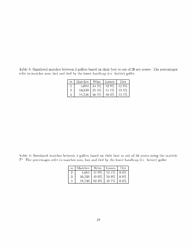
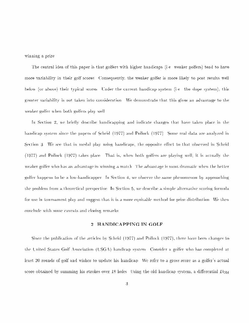
Table 3: Simulated matches between 2 golfers based on their best m out of 20 net scores. The percentagesrefer to matches won, lost and tied by the lower handicap (i.e. better) golfer.m Matches Wins Losses Ties2 4,684 34.3% 52.8% 12.8%3 10,539 35.4% 51.1% 13.5%4 18,736 36.5% 50.4% 13.1%Table 4: Simulated matches between 2 golfers based on their best m out of 20 scores using the statisticT �. The percentages refer to matches won, lost and tied by the lower handicap (i.e. better) golfer.m Matches Wins Losses Ties2 4,684 47.9% 52.1% 0.0%3 10,539 49.0% 50.9% 0.0%4 18,736 50.3% 49.7% 0.0%

19

•

•

••

••

•

••

•

•

• • •

••

•• •

•

•

•

•

• ••

•

•

•

••

••

•

•

•

•

•

•

•

• •

•

•

••

•

•

•

Handicap Index

Min

imum

Net

Sco

re

0 10 20 30

5055

6065

7075

80

Figure 1: Minimum Net Score Versus Handicap Index

20

•

•

•

•

• •

•

••

•

•

• ••

•

•

•

• ••

•

••

•

•

•

•

•

•

•

•

•

•

••

•

•

•

••••

•

•

•

•

•

•

•

Handicap Index

Sta

ndar

d D

evia

tion

of N

et S

core

s

0 10 20 30

02

46

810

Figure 2: Standard Deviation of Net Scores Versus Handicap Index

21

•

•

•

•

••

•

•

•••• •

•

••

•

•

•

•

••

•

•

•

•

•

•

•

•

•

•

••

•

•••

•• •

•

•

•

•

•

•

Handicap Index

Sta

ndar

d D

evia

tion

of D

iffer

entia

ls

0 10 20 30

02

46

8

Figure 3: Standard Deviation of Differentials Versus Handicap Index

22

•

•

••

• •

•

•

•

•

•

•

•

• •

•

•

•

•

•

•

•

•

•

•

•

•

•

•

•

•

•

•

•

•

•

•

•

•

•

•

•

•

•

•

•

•

•

•

Handicap Index

T*

0 10 20 30

-3-2

-10

Figure 4: Minimum T* Versus Handicap Index

23