Resistive Network Optimal Power Flow:Uniqueness and Algorithms

Chee Wei Tan,Senior Member, IEEE, Desmond W. H. Cai,Student Member, IEEEand Xin Lou

Abstract—The optimal power flow (OPF) problem minimizesthe power loss in an electrical network by optimizing the voltageand power delivered at the network buses, and is a nonconvexproblem that is generally hard to solve. By leveraging a recentdevelopment on the zero duality gap of OPF, we propose asecond-order cone programming convex relaxation of the resistivenetwork OPF, and study the uniqueness of the optimal solutionusing differential topology especially the Poincare–HopfIndexTheorem. We characterize the global uniqueness for differentnetwork topologies, e.g., line, radial and mesh networks. Thisserves as a starting point to design distributed local algorithmswith global behaviors that have low complexity, computationallyfast and can run under synchronous and asynchronous settingsin practical power grids.

I. I NTRODUCTION

The Optimal Power Flow (OPF) problem is a classicalnonlinear and nonconvex optimization problem that minimizesthe power generation costs and transmission loss in a powernetwork subject to physical constraints governed by Kirch-hoff’s and Ohm’s law [1]–[3]. There is a huge body of workon solving the OPF since Carpentier’s first formulation in 1962[1]. To overcome the nonlinearity and nonconvexity, the ma-jority of these work uses approximation methodologies to firstsimplify the OPF and then solve the approximated problem.For example, a popular approximation technique is the so-called DC OPF linearization that assumes a constant voltageand uses small angle approximation [4] and there are also othernumerically efficient approximation methods [5]–[12]. It is akey challenge to find new optimization methodologies that canovercome the nonconvexity barrier to solve the OPF optimallyand exactly, especially in a large-scale network.

Recent developments have shown that the OPF can beconvexified using a reformulation-relaxation technique andsemidefinite programming (SDP). We refer the readers to[14], [15] for an overview on this development that clarifiesthe relationships between various models of OPF and its

Manuscript received October 02, 2013; revised November 09,2013, andFebruary 14, 2014; accepted May 6, 2014. The work in this paper was partiallysupported by grants from the Research Grants Council of HongKong ProjectNo. RGC CityU 122013, ARPA-E grant DE-AR0000226 and the NationalScience Council of Taiwan, R.O.C. grant paper published in 2014: NSC 103-3113-P-008-001.

C. W. Tan is with the College of Science and Engineering, CityUniversityof Hong Kong, Tat Chee Ave., Hong Kong and a visiting professor withthe State Key Laboratory of Integrated Services Networks, Xidian University,China (email: cheewtan@cityu.edu.hk). D. W. H. Cai is with the Departmentof Electrical Engineering, California Institute of Technology, Pasadena, CA91125 USA (e-mail: wccai@caltech.edu). X. Lou is with the College ofScience and Engineering, City University of Hong Kong, HongKong.

convex relaxation. This is important because SDP is a convexoptimization problem that can be efficiently solved [16]. Inparticular, the authors in [17], [18] showed that the Lagrangeduality gap between the OPF problem and its convex dual canin fact be zero in a radial network, and this was numericallyverified to be true for a number of practical IEEE powernetworks. Specifically, this SDP convex relaxation problemisin fact tight1 when a certain load over-satisfaction conditionis assumed [17], [19]. The load over-satisfaction condition2

means that there is no lower bound on the real power consump-tion at each bus, and the power supplied to each bus in thenetwork can be greater than their respective power demands.

There are other recent work on reformulation-relaxationtechniques for the OPF. The author in [22] studied the con-vexification of the AC OPF using a branch flow model thatutilizes a second-order cone programming (SOCP) relaxationfor radial networks. The authors in [23] also proposed SOCPrelaxation that are applicable to AC OPF based on the SDPrelaxation work in [17], [18]. We note that, independent ofthe work in this paper and that in [23], an SOCP relaxationfor the resistive network was proposed in a recent paper [24],where the authors studied an SOCP relaxation without theaforementioned load over-satisfaction assumption but requir-ing an infinite voltage upper bound, which is different fromthe work in this paper. In addition, the solution uniquenessof the AC OPF that uses the SDP convex relaxation has alsobeen recently explored in [25].

In this paper, we leverage the developments in [17], [18]to further analyze the OPF problem in a purely resistivenetwork (i.e., without phase angle, reactive power variablesand reactance parameters). This kind of network can bepractically important and promising in HVDC (high-voltagedirect current) networks or microgrid clusters that integraterenewable energy sources (e.g., photovoltaic generator) thatproduce only real power. Indeed, studying the resistive net-work OPF and its algorithm design enables a deeper analysisof a problem with much simpler equations but still retaining

1We say that a relaxation is tight when the relaxation has an optimal valuethat is equal to the global optimal value of the original nonconvex problem,and an optimal primal solution of the original problem can beobtained froman optimal primal solution of the relaxation.

2In this paper, we study the OPF with the load over-satisfaction assumption,which implies the zero-duality gap condition. It is howeverimportant to findout the extent to which this assumption is true and indeed there are recentwork that study the limitations of this assumption (see, e.g., [20], [21]). It isinteresting to find other new conditions under which the OPF has zero dualitygap or can be convexified.

some of the important features of the general OPF, whosealgorithm development can potentially be used for a moregeneral OPF and the real applications [13]. We first proposean efficient SOCP relaxation of the resistive network OPFand prove its tightness under a monotonicity condition of thecost objective function. We then focus on the special case oftransmission power loss minimization in the resistive network,and characterize the uniqueness of its optimal solutions forvarious network topologies. This has implications on howdistributed algorithms can be designed to solve this lossminimization OPF problem. Our techniques and algorithmscan also be extended to solve other kinds of OPF problemformulation. As an example, our distributed algorithms canbe incorporated to solve a multi-period resistive network OPFwith energy storage [26].

Our algorithm design differs from prior work in the vastliterature, e.g., in [5]–[12], in the following aspects. Weleverage the zero duality gap results in [17] and dual decom-position to design decentralized algorithms in which each bus(either the generator bus or the demand bus) performs a localinformation (e.g., voltages and powers) update and can alsoexchange the local information with its one-hop neighbors(either synchronously or asynchronously). The uniquenesscharacterization provides an interesting perspective on theoptimal solution as well as the convergence proof of the localalgorithms to the global optimal solution.

Overall, the contributions of the paper are as follows:

1) We propose a SOCP convex relaxation for the resistivenetwork OPF and prove the tightness of this convexrelaxation under mild conditions.

2) We characterize the uniqueness of the resistive networkOPF solution using the Poincare-Hopf Index Theoremfor different network topologies, and we illustrate ourtechniques using various illustrative examples and nu-merical evaluation.

3) We leverage the uniqueness property to solve the re-sistive network OPF problem using dual decompositionand iterative fixed-point analysis. Computationally fastconvergent local algorithms with low complexity areproposed to compute the global optimal solution of theresistive network OPF in a distributed manner underboth synchronous and asynchronous settings.

II. SYSTEM MODEL AND PROBLEM FORMULATION

We consider a resistive power network with a set of busesN = f1; 2; : : : ; Ng and a set of transmission linesE � N �N . We model the power flow in the network using the businjection model that focuses on the voltage and the powerinjection at each bus of the network. We assume that eachbus is either a generation bus or a demand bus. A demandbus i can model the aggregate of users (loads) in a powernetwork. For each busi, we usei to represent the set ofbuses connecting to busi andjij � 1. Moreover, we assumethat the line admittance satisfiesYij = Yji 2 R+ , if (i; j) 2 E ;and Yij = Yji = 0, otherwise. In a purely resistive powernetwork, the admittance matrixY is given byY = G, where

G is the system conductance matrix. We assume that the graphof the power system is fully connected, i.e., there exists a pathbetween every two buses of the network. We useV and Ito denote the voltage magnitude vector(Vi)i2N and currentmagnitude vector(Ii)i2N respectively.

We consider nodal power and voltage constraints given byViIi � �pi and Vi 2 [V i; V i℄, 8i 2 N respectively. If busiis a generation bus, then�pi represents the generator capacityand �pi > 0. If bus i is a demand bus, then�pj < 0 and thisconstraint corresponds to the minimum demand that has to besatisfied at busi. We assume that demand can be over-satisfied,which is a practical assumption when there are power storagedevices available at the demand buses. Therefore, a demandbusi not only absorbsjpij amount of power, but it also absorbsadditional power to charge the power storage device attachedto it. Moreover, for each line(i; j) 2 E , we impose the linecapacity constraintGij(Vi � Vj)2 � ij . Then, the resistivenetwork OPF can be formulated as minimizing an objectivefunction f(I;V) (e.g., generation cost or transmission loss)over the resistive network subject to bus and line constraints:

minimize f(I;V)subject to IiVi � �pi 8i 2 N ;V i � Vi � V i 8i 2 N ;Gij(Vi � Vj)2 � ij 8(i; j) 2 E ;variables: Vi; Ii; i 2 N : (1)

By Ohm’s Law and Kirchhoff’s current law, we haveI = GV,i.e., 0BB� I1I2

...IN1CCA = 0BBBBB� Pj21G1j � � � �G1N�G21 � � � �G2N...

. . ....�GN1 � � � Pj2N GNj1CCCCCA0BB� V1V2

...VN1CCA : (2)

Substituting the above relationship betweenG and I into(1), the optimal power flow problem in (1) is equivalent to thefollowing optimization problem with quadratic constraints:

minimize f(V)subject to VTGiV � pi 8i 2 N ;V � V � V;VTGijV � ij 8(i; j) 2 E ;variables: V; (3)

whereGi = 12 (EiG +GEi) andGij = Gij(ei � ej)(ei �ej)T , whereei is the standard basis vector inRn andEi =eieTi 2 Rn�n [17]. Let the optimal solution of (3) beV�.Since (3) is nonconvex, it is generally hard to solve forV�.

III. SECOND-ORDER CONE PROGRAMMING CONVEX

RELAXATION

In this section, we propose a SOCP convex relaxation of (3),which is in fact tight under mild conditions on the objectivefunction f(V). Let us first introduce the auxiliary variablesWii = V 2i ; 8i 2 N andWij = ViVj 8(i; j) 2 E . We shallalso use the nonnegative matrixW to represent(Wii)i2N

and (Wij)(i;j)2E . We rewrite the objective functionf(V) interms of the auxiliary variables to obtainf(W), so that (3) isequivalent to the following optimization problem:

minimize f(W)subject to

Pj2iGij(Wii �Wij) � �pi 8i 2 N ;V 2i �Wii � V 2i 8i 2 N ;Gij(Wii +Wjj � 2Wij) � ij 8(i; j) 2 E ;WiiWjj = W 2ij 8(i; j) 2 E ;Wij � 0; Wji � 0 8(i; j) 2 E ;variables: W: (4)

Let the optimal solution of (4) beW�. Now, observe that allthe constraints in (4) are convex inW except for the equalityconstraintsWiiWjj = W 2ij 8(i; j) 2 E . We consider relax-ing these nonconvex constraints into the following inequalityconstraints: WiiWjj �W 2ij 8(i; j) 2 E ; (5)

which are equivalent to the following SOCP constraints:�������� 2WijWii �Wjj ��������2 �Wii +Wjj 8(i; j) 2 E : (6)

Lemma 1:Suppose thatf(W) is monotonically decreasingin Wij ;8(i; j) 2 E . Then, the relaxation of the resistivenetwork OPF in (4) with SOCP constraints (6) is tight, andfurthermoreW� = V�V� T .

Proof: To prove the tightness of the SOCP relaxation,we show that there exists an optimal solution such that theconstraints (5) are active, i.e., the inequalities become strictlyequalities. Suppose thatW� is an optimal solution of therelaxed problem and there exists a line(`1; `2) 2 E such thatthe constraintW �1`1W �2`2 � W �2`1`2 is inactive, i.e., a strictinequality. Sincef(W) is decreasing inWij ;8(i; j) 2 E ,we can choose someW such thatW �1`1W �2`2 = W 21`2 =W �2`1`2 + � > W �2`1`2 holds. SinceGij > 0;W = W is feasibleand gives a smaller objective value (contradicting the factthatW� is optimal), it is also an optimal solution.

Remark 1: If f(W) is convex, then the SOCP relaxation of(4) is also convex and its duality gap is zero under mild con-ditions (Slater’s conditions being satisfied) [16]. In addition,the SOCP relaxation of (4) can be solved by interior-pointmethods that have a much better worst case complexity thantheir SDP counterparts [16], and there are widely-availablestandard optimization packages (e.g., see [27]) that can solveSOCP efficiently.

In fact, observe that the transmission loss minimizationsatisfies the condition imposed on the objective function inLemma 1 since, in the transmission loss minimization setting,we consider a quadratic objective functionf(V) = VTGV(making f(W) linearly decreasing inWij ). In the following,for simplicity and clarity, we shall focus on this objectivefunction f(V) = VTGV, and study the uniqueness of theoptimal solution in (3) with ramification on the design ofdistributed algorithms to solve (3).

IV. U NIQUENESSCHARACTERIZATION

In this section, we study the uniqueness of the solution to(3). The uniqueness characterization of (3) has implicationson how local algorithms with low complexity can be designedto solve (3) (see Section V). Our approach is to leveragethe zero duality gap property in (3) and the Poincare-HopfIndex Theorem in [28], [29] together with the nonnegativityassociated with the variables and problem parameters of (3).

We first use the Lagrange dual decomposition to relax (3).Define the following partial Lagrangian function:L(V; f�;�g) := X(i;j)2E(�i + 1)GijVi(Vi � Vj)�Xi2N �ipi+ X(i;j)2E �ijGij(Vi � Vj)2 � X(i;j)2E �ij ij ;where� and� are the nonnegative dual variables associatedwith the constraintsVTGjV � pi 8i 2 N andVTGijV � ij 8(i; j) 2 E respectively. For any given feasible�i ateach bus and�ij at each line, consider the following partialLagrangian minimization problem:

minimize L(V; f�;�g)subject to V i � Vi � V i 8i 2 N : (7)

Note that (7) is nonconvex inV. However, since the objectiveis smooth and by using the Slater’s condition that guaranteesthe existence of the interior of a feasible constraint set, theoptimal solution to (7) must satisfy the Karush-Kuhn Tucker(KKT) conditions. By rewriting the KKT conditions, it can beshown that the optimal solution must satisfy:V = max�V;min�V;B(�;�)V ; (8)

where the nonnegative matrixB3 has entries in terms of�and�:Bij = 8><>: 2Gij+�iGij+�jGij+2�ijGij2 (1+�i) Pj2i Gij+ P(i0;j0)2E �i0j0Gi0j0! 8(i; j) 2 E0 otherwise:

(9)Suppose that the optimal dual variables�� and �� of (3)are given (recall that they exist due to the zero dualitygap), then the optimal voltageV� must satisfyV� =max�V;min�V;B(��;��)V�.

It is interesting to ask whetherV� is unique. There areseveral ramifications to the solvability of (3) by the convexre-laxation (4) and also to solving (3) using distributed algorithms(also see Remark 3 later). To prove uniqueness, we leveragea result in [28], [29] to inspect the generalized critical pointsof rL(V; f�;�g) (the first order derivative ofL(V; f�;�g)with respect toV) over the box constraint set in(7). We firststate the definition of the P-matrix and the result in [28].

3The nonnegative matrixB is irreducible since the graph of the powernetwork is fully connected, i.e.,G is irreducible. By the Perron-Frobeniustheorem (cf. Proposition 6.6 in [31]), its spectral radius�(B) is an eigenvalueof B (the Perron-Frobenius eigenvalue). Also,�(B) is simple and positive,and the right and left eigenvectors corresponding to�(B) are positive.

Definition 1 ( [28], Definition 1): An n� n matrix A is aP-matrix if all the determinants of its principal sub-matricesare positive, i.e.det(AjJ) > 0, 8J � f1; 2; : : : ; ng.

Lemma 2 ( [28], Corollary 1):Let M be a box-constrained region. LetU be an open set containingM , and f : U ! R be a twice differentiable function.Let KKT (f;M) denote the Karush-Kuhn-Tucker stationarypoints of f over the regionM and assume that forevery x 2 KKT(f;M); H(x)jIrf (x) is a P-matrix, whereH(x)jIrf (x) denotes the principal submatrix of the Hessianmatrix H(x) containing precisely the entriesHij wherei; j 2 Irf (x) and Irf (x) = fi 2 f1; 2; : : : ; Ngjrfi = 0g.Then, KKT(f;M) has a unique element which is also theunique local (global) minimum off overM .

Now, the derivative ofrL(V; f�;�g), i.e., the Hessianin (7), is given by a square matrix in terms off�;�g. Letus denote this Hessian matrix byA. Clearly, the uniquenessof the solution in (3) depends on the network topology (asA containsG and Gij) and the dual variables (how theypair up with the optimal primal variableV� to satisfy theKKT conditions). In the following, we study the applicationof Lemma 2 to this Hessian matrixA using simple networktopologies for illustration.

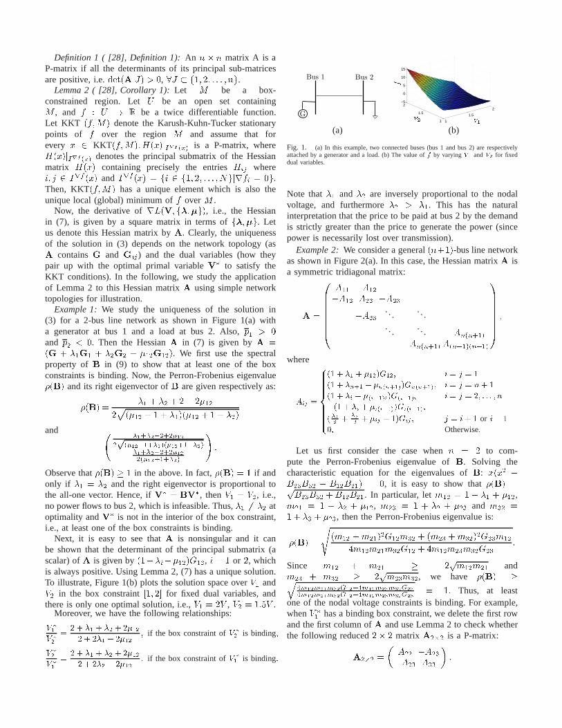
Example 1:We study the uniqueness of the solution in(3) for a 2-bus line network as shown in Figure 1(a) witha generator at bus 1 and a load at bus 2. Also,p1 > 0and p2 < 0. Then the HessianA in (7) is given byA =(G + �1G1 + �2G2 + �12G12). We first use the spectralproperty ofB in (9) to show that at least one of the boxconstraints is binding. Now, the Perron-Frobenius eigenvalue�(B) and its right eigenvector ofB are given respectively as:�(B) = �1 + �2 + 2 + 2�122p(�12 + 1 + �1)(�12 + 1 + �2)and �1+�2+2+2�122p(�12+1+�1)(�12+1+�2)�1+�2+2+2�122(�12+1+�2) ! :Observe that�(B) � 1 in the above. In fact,�(B) = 1 if andonly if �1 = �2 and the right eigenvector is proportional tothe all-one vector. Hence, ifV� = BV�, thenV1 = V2, i.e.,no power flows to bus 2, which is infeasible. Thus,�1 6= �2 atoptimality andV� is not in the interior of the box constraint,i.e., at least one of the box constraints is binding.

Next, it is easy to see thatA is nonsingular and it canbe shown that the determinant of the principal submatrix (ascalar) ofA is given by(1+�i+�12)G12, i = 1 or 2, whichis always positive. Using Lemma 2, (7) has a unique solution.To illustrate, Figure 1(b) plots the solution space overV1 andV2 in the box constraint[1; 2℄ for fixed dual variables, andthere is only one optimal solution, i.e.,V1 = 2V , V2 = 1:5V .

Moreover, we have the following relationships:V �1V �2 = 2 + �1 + �2 + 2�122 + 2�1 + 2�12 ; if the box constraint ofV �2 is binding;V �2V �1 = 2 + �1 + �2 + 2�122 + 2�2 + 2�12 ; if the box constraint ofV �1 is binding:

G

Bus 1 Bus 2

1

1.5

2

1

1.5

2−5

0

5

10

15f V1V2(a) (b)

Fig. 1. (a) In this example, two connected buses (bus 1 and bus 2) are respectivelyattached by a generator and a load. (b) The value off by varyingV1 andV2 for fixeddual variables.

Note that�1 and �2 are inversely proportional to the nodalvoltage, and furthermore�2 > �1. This has the naturalinterpretation that the price to be paid at bus 2 by the demandis strictly greater than the price to generate the power (sincepower is necessarily lost over transmission).

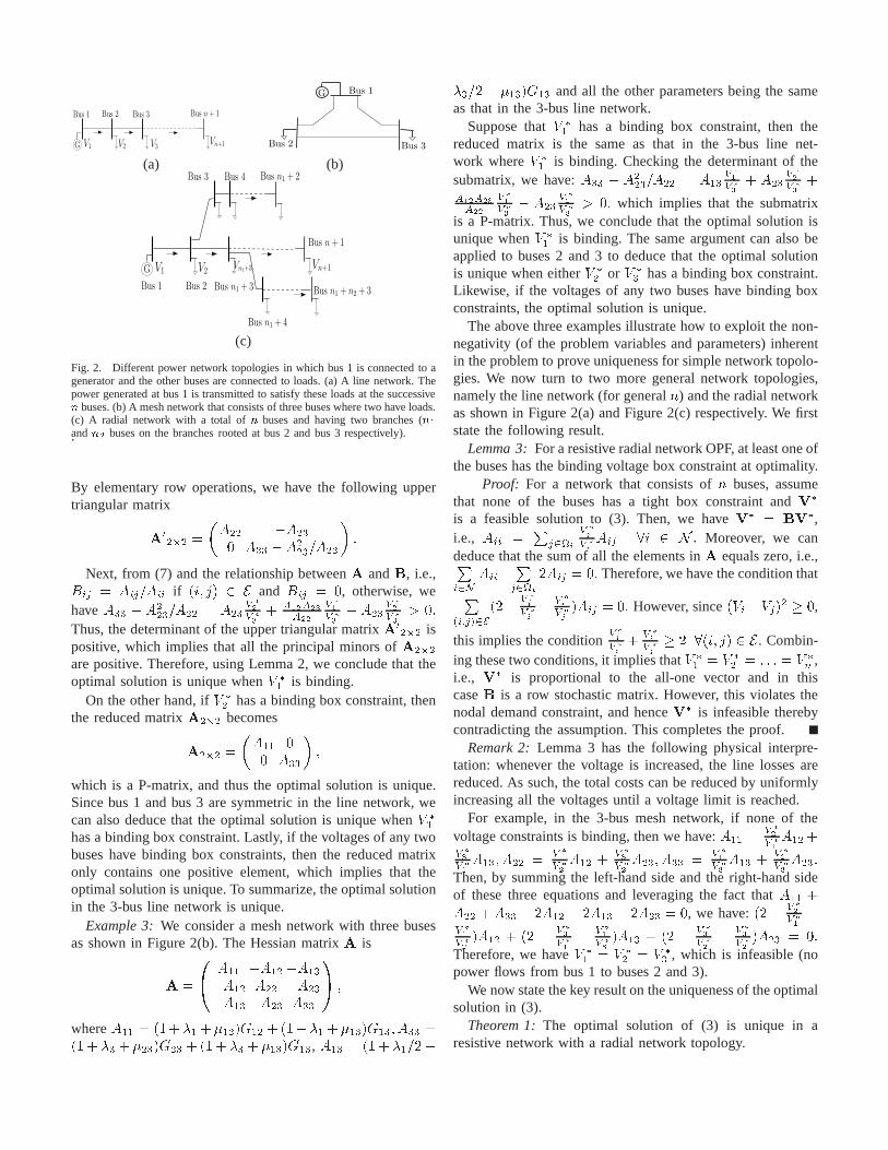
Example 2:We consider a general(n+1)-bus line networkas shown in Figure 2(a). In this case, the Hessian matrixA isa symmetric tridiagonal matrix:A = 0BBBBBB� A11 �A12�A12 A22 �A23�A23 . . .

. . .. . .

. . . �An(n+1)�An(n+1) A(n+1)(n+1)1CCCCCCA ;

whereAij = 8>>>>>>><>>>>>>>:(1 + �1 + �12)G12; i = j = 1(1 + �n+1 + �n(n+1))Gn(n+1); i = j = n+ 1(1 + �i + �(i�1)i)G(i�1)i i = j = 2; : : : ; n+(1 + �i + �i(i+1))Gi(i+1);(�i2 + �j2 + �ij + 1)Gij ; j = i+ 1 or i� 10; Otherwise:Let us first consider the case whenn = 2 to com-

pute the Perron-Frobenius eigenvalue ofB. Solving thecharacteristic equation for the eigenvalues ofB: x(x2 �B23B32 � B12B21) = 0, it is easy to show that�(B) =pB23B32 +B12B21. In particular, letm12 = 1 + �1 + �12,m21 = 1 + �2 + �12, m23 = 1 + �2 + �23 and m32 =1 + �3 + �23, then the Perron-Frobenius eigenvalue is:�(B) =s (m12 +m21)2G12m32 + (m23 +m32)2G23m124m12m21m32G12 + 4m12m23m32G23 :Since m12 + m21 � 2pm12m21 andm23 + m32 � 2pm23m32, we have �(B) �q 4m12m21m32G12+4m12m23m32G234m12m21m32G12+4m12m23m32G23 = 1: Thus, at leastone of the nodal voltage constraints is binding. For example,whenV �1 has a binding box constraint, we delete the first rowand the first column ofA and use Lemma 2 to check whetherthe following reduced2� 2 matrixA2�2 is a P-matrix:A2�2 = � A22 �A23�A23 A33 � :

V1 V2 V3Vn+1G

Bus 1 Bus 2 Bus 3 Bus n+ 1

G Bus 1

Bus 2 Bus 3

(a) (b)

V1 V2Vn+1G

Bus 1 Bus 2

Bus 3

Bus n+ 1

Bus 4 Bus n1 + 2

Vn1+3

Bus n1 + 4

Bus n1 + n2 + 3Bus n1 + 3

(c)

Fig. 2. Different power network topologies in which bus 1 is connected to agenerator and the other buses are connected to loads. (a) A line network. Thepower generated at bus 1 is transmitted to satisfy these loads at the successiven buses. (b) A mesh network that consists of three buses where two have loads.(c) A radial network with a total ofn buses and having two branches (n1andn2 buses on the branches rooted at bus 2 and bus 3 respectively)..

By elementary row operations, we have the following uppertriangular matrixA02�2 = �A22 �A230 A33 �A223=A22� :

Next, from (7) and the relationship betweenA andB, i.e.,Bij = Aij=Aii if (i; j) 2 E and Bij = 0, otherwise, wehaveA33 � A223=A22 = A23 V �2V �3 + A12A23A22 V �1V �3 � A23 V �2V �3 > 0:Thus, the determinant of the upper triangular matrixA02�2 ispositive, which implies that all the principal minors ofA2�2are positive. Therefore, using Lemma 2, we conclude that theoptimal solution is unique whenV �1 is binding.

On the other hand, ifV �2 has a binding box constraint, thenthe reduced matrixA2�2 becomesA2�2 = �A11 00 A33� ;which is a P-matrix, and thus the optimal solution is unique.Since bus 1 and bus 3 are symmetric in the line network, wecan also deduce that the optimal solution is unique whenV �3has a binding box constraint. Lastly, if the voltages of any twobuses have binding box constraints, then the reduced matrixonly contains one positive element, which implies that theoptimal solution is unique. To summarize, the optimal solutionin the 3-bus line network is unique.

Example 3:We consider a mesh network with three busesas shown in Figure 2(b). The Hessian matrixA isA = 0� A11 �A12 �A13�A12 A22 �A23�A13 �A23 A33 1A ;whereA11 = (1+�1+�12)G12 +(1+�1+�13)G13; A33 =(1+ �3 +�23)G23 + (1+ �3 + �13)G13, A13 = (1+ �1=2+

�3=2 + �13)G13 and all the other parameters being the sameas that in the 3-bus line network.

Suppose thatV �1 has a binding box constraint, then thereduced matrix is the same as that in the 3-bus line net-work whereV �1 is binding. Checking the determinant of thesubmatrix, we have:A33 � A223=A22 = A13 V �1V �3 + A23 V �2V �3 +A12A23A22 V �1V �3 � A23 V �2V �3 > 0; which implies that the submatrixis a P-matrix. Thus, we conclude that the optimal solution isunique whenV �1 is binding. The same argument can also beapplied to buses 2 and 3 to deduce that the optimal solutionis unique when eitherV �2 or V �3 has a binding box constraint.Likewise, if the voltages of any two buses have binding boxconstraints, the optimal solution is unique.

The above three examples illustrate how to exploit the non-negativity (of the problem variables and parameters) inherentin the problem to prove uniqueness for simple network topolo-gies. We now turn to two more general network topologies,namely the line network (for generaln) and the radial networkas shown in Figure 2(a) and Figure 2(c) respectively. We firststate the following result.

Lemma 3:For a resistive radial network OPF, at least one ofthe buses has the binding voltage box constraint at optimality.

Proof: For a network that consists ofn buses, assumethat none of the buses has a tight box constraint andV�is a feasible solution to (3). Then, we haveV� = BV�,i.e., Aii = Pj2i V �jV �i Aij 8i 2 N : Moreover, we candeduce that the sum of all the elements inA equals zero, i.e.,Pi2N Aii� Pj2i 2Aij = 0: Therefore, we have the condition thatP(i;j)2E(2� V �jV �i � V �iV �j )Aij = 0: However, since(Vi�Vj)2 � 0,

this implies the conditionV �jV �i + V �iV �j � 2 8(i; j) 2 E . Combin-

ing these two conditions, it implies thatV �1 = V �2 = : : : = V �n ,i.e., V� is proportional to the all-one vector and in thiscaseB is a row stochastic matrix. However, this violates thenodal demand constraint, and henceV� is infeasible therebycontradicting the assumption. This completes the proof.

Remark 2:Lemma 3 has the following physical interpre-tation: whenever the voltage is increased, the line losses arereduced. As such, the total costs can be reduced by uniformlyincreasing all the voltages until a voltage limit is reached.

For example, in the 3-bus mesh network, if none of thevoltage constraints is binding, then we have:A11 = V �2V �1 A12+V �3V �1 A13; A22 = V �1V �2 A12 + V �3V �2 A23; A33 = V �1V �3 A13 + V �2V �3 A23:Then, by summing the left-hand side and the right-hand sideof these three equations and leveraging the fact thatA11 +A22 +A33 � 2A12 � 2A13 � 2A23 = 0, we have:(2� V �2V �1 �V �1V �2 )A12 + (2 � V �3V �1 � V �1V �3 )A13 + (2 � V �3V �2 � V �3V �2 )A23 = 0:Therefore, we haveV �1 = V �2 = V �3 , which is infeasible (nopower flows from bus 1 to buses 2 and 3).

We now state the key result on the uniqueness of the optimalsolution in (3).

Theorem 1:The optimal solution of (3) is unique in aresistive network with a radial network topology.

Remark 3:There are several implications on the uniquenessof V�. Note that (8) implies that the Lagrange dual functionis smooth at the optimality of (3). The smoothness of theLagrange dual at optimality implies that the optimal dualvariables are unique and stable, and thus can be suitably usedas power and line prices in pricing schemes. More importantly,it enlarges the space of designing simple local algorithmswith low complexity to solve (3), and we address this in thefollowing section.

V. L OCAL ALGORITHMS

In this section, we design simple local algorithms to solve(3). This is achieved by first solving (7) for givenf�;�g, andthen using the projected gradient method in [30] to update thedual variables, which in turn are used as the input to solving(7) iteratively.

We propose the following fixed point algorithmthat computes the fixed pointV in (8) for agiven set of feasible dual variables� and �.

Algorithm 1:

Compute voltageV:Vi(k + 1) = max8<:V i;min8<:V i; Xj2i BijVj(k)9=;9=; ; (10)

for all i 2 N , whereBij is given in (9) for alli; j.Theorem 2:Suppose (7) has a unique optimal solution.

Then, given anyV(0) which satisfiesV � V(0) � V, V(k)in Algorithm 1 converges to the unique optimal solution of (7).

Proof: Let f(V) = max�V;min�V;BV. First, weshow that ifV(0) = V, thenV(k) is a monotonic increasingand bounded sequence. Clearly, we haveV(1) � f(V(0)) �V = V(0): Now, observe that for anyV(k) andV(k + 1)satisfyingV(k + 1) � V(k), we haveV(k + 2) = f(V(k + 1)) � f(V(k)) = V(k + 1): (11)

Here, the inequality follows from the fact that the entries ofB are nonnegative. By induction, it follows thatV(k) is amonotonic increasing sequence. Clearly,V(k) = f(V(k �1)) � V for all k so it is bounded.

By a similar argument, we have that ifV(0) = V, thenV(k) is a monotonic decreasing and bounded sequence.Now, given anyV(0) which satisfiesV � V(0) � V, we

have limk!1 fk(V) � limk!1 fk(V(0)) � limk!1 fk(V): (12)

Sincefk(V) is a monotonic increasing and bounded sequence,it must converge. By Theorem 1 there is a unique solution toV = f(V). Hencefk(V) must converge to the unique fixedpoint. Let us denote byV� the unique fixed point. Using asimilar argument, we conclude thatfk(V) must also convergetoV�. Hence, we haveV� � limk!1 fk(V(0)) � V�, whichimplies thatlimk!1 fk(V(0)) = V�.

Due to practical considerations on information exchangeand computation time at each bus, some of the buses mayexecute less iterations or use outdated and asynchronous iter-ates for update. In the following, we study the asynchronousversion of Algorithm 1.

Assumption 1:(Total asynchronism, [31], pp.430) Denote� ij (k) as the most recent time forVj that is known to busi, where0 < � ij (k) < k, andKi as the set of times whereVi(k) is updated, i.e.,Vi(k) is unchanged at timesk 62 Vi(k).Assume the setsKi are infinite. Ifkt is a sequence of elementsof Ki that tends to infinity, thenlimt!1 � ij (kt) =1 for everyj.Using Assumption 1, the convergence of the asynchronousversion of Algorithm 1 is determined in the following:

Corollary 1: Suppose (7) has a unique optimal solution.Then, from any initialV(0) which satisfiesV � V(0) � V,V(k) in the totally asynchronous version of Algorithm 1converges to the unique optimal solution of (7).

We next leverage Algorithm 1 together with a gra-dient projection method in [30] that updates the dualvariables � and � to solve (7) in the following.

Algorithm 2:

1) Set the stepsizes�; � 2 (0; 1).2) Run Algorithm 1 with input�i(t) and �ij(t) for the

entries ofB.3) Compute:�i(t+ 1) = maxf0; �i(t)+�(Xj2iGijVi(k)(Vi(k)�Vj(k))�pi)g;

(13)for all i 2 N .�ij(t+ 1) = maxf0; �ij(t)+�(Gij(Vi(k)�Vj(k))2� ij)g; (14)

for all (i; j) 2 E :Update the stepsizes� and� according to Theorem 3.

Theorem 3:Assume thatVi(k) and Vi(k) denote the (pre-maturely terminated) approximated and the exact solution (onconvergence) at step 2 of Algorithm 2 for�i(t) and �ij(t),respectively. Suppose the output of Algorithm 1 satisfiesXi2N lim supk jXj2iGij Vi(k)(Vi(k)� Vj(k))� pij � �1and X(i;j)2E lim supk jGij(Vj(k)� Vi(k))2 � ij j � �2for some sufficiently small positive�1 and�2. We choose thediminishing stepsizes�(t) and�(t) to satisfy1Xt=0 �(t) =1; 1Xt=0(�(t))2 <1; 1Xt=0 �(t) =1; 1Xt=0(�(t))2 <1:Then�(t+1) and�(t+1) converge to a closed neighborhoodof �� and�� when t!1, respectively.

G G

Bus 1

Bus 2 Bus 3

Bus 4 Bus 5

V2(k), λ2(t){ }

V4(k), λ4(t){ } V5(k), λ5(t){ }

V3(k), λ3(t){ }

V1(k), λ1(t){ }

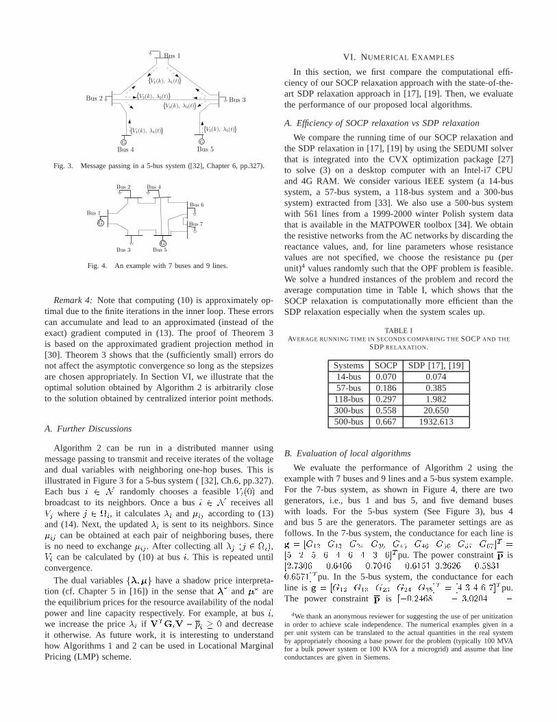
Fig. 3. Message passing in a 5-bus system ([32], Chapter 6, pp.327).

Bus 1

Bus 2

Bus 3

Bus 4

Bus 5

G

G

Bus 6

Bus 7

Fig. 4. An example with 7 buses and 9 lines.

Remark 4:Note that computing (10) is approximately op-timal due to the finite iterations in the inner loop. These errorscan accumulate and lead to an approximated (instead of theexact) gradient computed in (13). The proof of Theorem 3is based on the approximated gradient projection method in[30]. Theorem 3 shows that the (sufficiently small) errors donot affect the asymptotic convergence so long as the stepsizesare chosen appropriately. In Section VI, we illustrate thattheoptimal solution obtained by Algorithm 2 is arbitrarily closeto the solution obtained by centralized interior point methods.

A. Further Discussions

Algorithm 2 can be run in a distributed manner usingmessage passing to transmit and receive iterates of the voltageand dual variables with neighboring one-hop buses. This isillustrated in Figure 3 for a 5-bus system ( [32], Ch.6, pp.327).Each busi 2 N randomly chooses a feasibleVi(0) andbroadcast to its neighbors. Once a busi 2 N receives allVj wherej 2 i, it calculates�i and�ij according to (13)and (14). Next, the updated�i is sent to its neighbors. Since�ij can be obtained at each pair of neighboring buses, thereis no need to exchange�ij . After collecting all�j (j 2 i),Vi can be calculated by (10) at busi. This is repeated untilconvergence.

The dual variablesf�;�g have a shadow price interpreta-tion (cf. Chapter 5 in [16]) in the sense that�� and�� arethe equilibrium prices for the resource availability of thenodalpower and line capacity respectively. For example, at busi,we increase the price�i if VTGiV � pi � 0 and decreaseit otherwise. As future work, it is interesting to understandhow Algorithms 1 and 2 can be used in Locational MarginalPricing (LMP) scheme.

VI. N UMERICAL EXAMPLES

In this section, we first compare the computational effi-ciency of our SOCP relaxation approach with the state-of-the-art SDP relaxation approach in [17], [19]. Then, we evaluatethe performance of our proposed local algorithms.

A. Efficiency of SOCP relaxation vs SDP relaxation

We compare the running time of our SOCP relaxation andthe SDP relaxation in [17], [19] by using the SEDUMI solverthat is integrated into the CVX optimization package [27]to solve (3) on a desktop computer with an Intel-i7 CPUand 4G RAM. We consider various IEEE system (a 14-bussystem, a 57-bus system, a 118-bus system and a 300-bussystem) extracted from [33]. We also use a 500-bus systemwith 561 lines from a 1999-2000 winter Polish system datathat is available in the MATPOWER toolbox [34]. We obtainthe resistive networks from the AC networks by discarding thereactance values, and, for line parameters whose resistancevalues are not specified, we choose the resistance pu (perunit)4 values randomly such that the OPF problem is feasible.We solve a hundred instances of the problem and record theaverage computation time in Table I, which shows that theSOCP relaxation is computationally more efficient than theSDP relaxation especially when the system scales up.

TABLE IAVERAGE RUNNING TIME IN SECONDS COMPARING THESOCPAND THE

SDPRELAXATION .

Systems SOCP SDP [17], [19]14-bus 0.070 0.07457-bus 0.186 0.385118-bus 0.297 1.982300-bus 0.558 20.650500-bus 0.667 1932.613

B. Evaluation of local algorithms

We evaluate the performance of Algorithm 2 using theexample with 7 buses and 9 lines and a 5-bus system example.For the 7-bus system, as shown in Figure 4, there are twogenerators, i.e., bus 1 and bus 5, and five demand buseswith loads. For the 5-bus system (See Figure 3), bus 4and bus 5 are the generators. The parameter settings are asfollows. In the 7-bus system, the conductance for each line isg = [G12 G13 G24 G35 G45 G46 G56 G57 G67℄T =[5 2 5 6 4 6 4 3 6℄Tpu. The power constraintp is[2:7306 �0:6466 �0:7046 �0:6151 3:2626 �0:5831 �0:6571℄Tpu. In the 5-bus system, the conductance for eachline is g = [G12 G13 G23 G24 G35℄T = [4 3 4 6 7℄Tpu.The power constraintp is [�0:2468 � 3:0204 �

4We thank an anonymous reviewer for suggesting the use of per unitizationin order to achieve scale independence. The numerical examples given in aper unit system can be translated to the actual quantities inthe real systemby appropriately choosing a base power for the problem (typically 100 MVAfor a bulk power system or 100 KVA for a microgrid) and assume that lineconductances are given in Siemens.

0 50 100 1501.05

1.1

1.15

1.2

1.25

1.3

1.35

1.4

1.45

1.5

iteration

Volta

ge (p

u)Evolution of voltage at loads with high capacities

Bus2(Algo 2)Bus4(Algo 2)Bus6(Algo 2)Bus2(optimal)Bus4(optimal)Bus6(optimal)

0 20 40 60 801

1.1

1.2

1.3

1.4

1.5

1.6

1.7

1.8

iteration

Volta

ge (p

u)

Evolution of voltage at generators with high capacities

Bus1(Algo 2)Bus5(Algo 2)Bus1(optimal)Bus5(optimal)

0 50 100 150 200 250 3001.05

1.1

1.15

1.2

1.25

1.3

1.35

1.4

iteration

Volta

ge (p

u)

Evolution of voltage at loads with low capacities

Bus2(Algo 2)Bus4(Algo 2)Bus6(Algo 2)Bus2(optimal)Bus4(optimal)Bus6(optimal)

0 50 100 150 200 250 300 3501.2

1.3

1.4

1.5

1.6

1.7

iteration

Volta

ge (p

u)

Evolution of voltage at generators with low capacities

Bus1(Algo 2)Bus5(Algo 2)Bus1(optimal)Bus5(optimal)

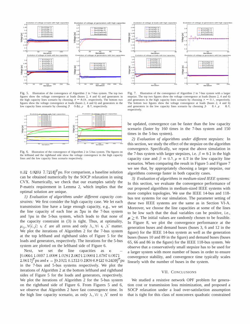
Fig. 5. Illustration of the convergence of Algorithm 2 in 7-bus system. The top twofigures show the voltage convergence at loads (buses 2, 4 and 6) and generators inthe high capacity lines scenario by choosing� = 0:01, respectively. The bottom twofigures show the voltage convergence at loads (buses 2, 4 and 6) and generators in thelow capacity lines scenario by choosing� = 0:05; � = 0:2, respectively.

0 50 100 150

1.1

1.2

1.3

1.4

1.5

1.6

1.7

1.8

1.9

Volta

ge (p

u)

Evolution of voltage with high capacities

Bus1(Algo 2)Bus2(Algo 2)Bus3(Algo 2)Bus4(Algo 2)Bus5(Algo 2)Bus1(optimal)Bus2(optimal)Bus3(optimal)Bus4(optimal)Bus5(optimal)

iteration0 50 100 150 200 250 300

1.1

1.2

1.3

1.4

1.5

1.6

1.7

1.8

1.9

iteration

Volta

ge (p

u)

Evolution of voltage with low capacities

Bus1(Algo 2)Bus2(Algo 2)Bus3(Algo 2)Bus4(Algo 2)Bus5(Algo 2)Bus1(optimal)Bus2(optimal)Bus3(optimal)Bus4(optimal)Bus5(optimal)

Fig. 6. Illustration of the convergence of Algorithm 2 in 5-bus system. The figures onthe lefthand and the righthand side show the voltage convergence in the high capacitylines and the low capacity lines scenario respectively.0:32 4:0203 7:7234℄Tpu. For comparison, a baseline solutioncan be obtained numerically by the SOCP relaxation in usingCVX. Numerically, we check that our examples satisfy theP-matrix requirement in Lemma 2, which implies that theoptimal solution are unique.

1) Evaluation of algorithms under different capacity con-straints: We first consider the high capacity case. We let eachtransmission line have a large enough capacity, e.g., we setthe line capacity of each line as3pu in the 7-bus systemand 1pu in the 5-bus system, which leads to that none ofthe capacity constraint in (3) is tight. Thus, at optimality,�ij ;8(i; j) 2 E are all zeros and only�i;8i 2 N matter.We plot the iterations of Algorithm 2 for the 7-bus systemat the top lefthand and righthand sides of Figure 5 for theloads and generators, respectively. The iterations for the5-bussystem are plotted on the lefthand side of Figure 6.

Next, we set the line capacities as =[0:0664 1:0097 1:0008 1:0284 2:0624 2:0004 1:0707 0:06712:0017℄Tpu and = [0:1021 0:1313 0:1938 0:8432 0:3459℄Tpuin the 7-bus and 5-bus systems respectively. We plot theiterations of Algorithm 2 at the bottom lefthand and righthandsides of Figure 5 for the loads and generators, respectively.We plot the iterations of Algorithm 2 for the 5-bus systemon the righthand side of Figure 6. From Figures 5 and 6,we observe that Algorithm 2 have fast convergence time. Inthe high line capacity scenario, as only�i;8i 2 N need to

0 15 301.05

1.1

1.15

1.2

1.25

1.3

1.35

1.4

1.45

1.5

iteration

Volta

ge (p

u)

Evolution of voltage at loads with high capacities

Bus2(Algo 2)Bus4(Algo 2)Bus6(Algo 2)Bus2(optimal)Bus4(optimal)Bus6(optimal)

0 10 20

1.1

1.2

1.3

1.4

1.5

1.6

iteration

Volta

ge (p

u)

Evolution of voltage at generators with high capacities

Bus1(Algo 2)Bus5(Algo 2)Bus1(optimal)Bus5(optimal)

0 50 1001.05

1.1

1.15

1.2

1.25

1.3

1.35

1.4

1.45

1.5

1.55

iteration

Volta

ge (p

u)

Evolution of voltage at loads with low capacities

Bus2(Algo 2)Bus4(Algo 2)Bus6(Algo 2)Bus2(optimal)Bus4(optimal)Bus6(optimal)

0 50 100 150 2001.2

1.3

1.4

1.5

1.6

iteration

Volta

ge (p

u)

Evolution of voltage at generators with low capacities

Bus1(Algo 2)Bus5(Algo 2)Bus1(optimal)Bus5(optimal)

Fig. 7. Illustration of the convergence of Algorithm 2 in 7-bus system with a largerstepsize. The top two figures show the voltage convergence atloads (buses 2, 4 and 6)and generators in the high capacity lines scenario by choosing � = 0:1, respectively.The bottom two figures show the voltage convergence at loads (buses 2, 4 and 6)and generators in the low capacity lines scenario by choosing � = 0:1; � = 0:2,respectively.

be updated, convergence can be faster than the low capacityscenario (faster by 160 times in the 7-bus system and 150times in the 5-bus system).

2) Evaluation of algorithms under different stepsizes:Inthis section, we study the effect of the stepsize on the algorithmconvergence. Specifically, we repeat the above simulation inthe 7-bus system with larger stepsizes, i.e.� = 0:1 in the highcapacity case and� = 0:1; � = 0:2 in the low capacity linescenarios. When comparing the result in Figure 5 and Figure 7we see that, by appropriately choosing a larger stepsize, ouralgorithms converge faster in both capacity cases.

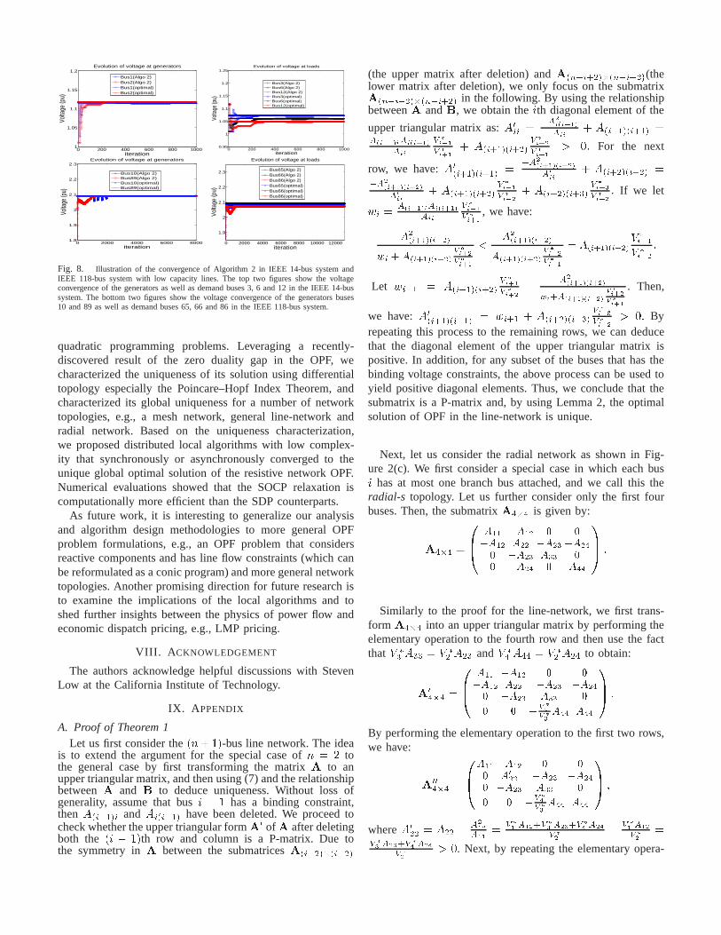
3) Evaluation of algorithms in medium-sized IEEE systems:In this section, we evaluate the convergence performance ofour proposed algorithms in medium-sized IEEE systems withmore complex topologies. We use the IEEE 14-bus and 118-bus test systems for our simulation. The parameter setting ofthese two IEEE systems are the same as in Section VI-A.Moreover, we choose the line capacities at some of the linesto be low such that the dual variables can be positive, i.e.,� � 0. The initial values are randomly chosen to be feasible.In Figure 8, we plot the convergence performance at thegeneration buses and demand buses (buses 3, 6 and 12 in thefigure) for the IEEE 14-bus system as well as the generationbuses (buses 10 and 89 in the figure) and demand buses (buses65, 66 and 86 in the figure) for the IEEE 118-bus system. Weobserve that a conservatively small stepsize has to be used fora larger system with more number of buses in order to ensureconvergence stability, and convergence time typically scaleslinearly with the number of buses in the system.

VII. C ONCLUSIONS

We studied a resistive network OPF problem for genera-tion cost or transmission loss minimization, and proposed aSOCP relaxation under a load over-satisfaction assumptionthat is tight for this class of nonconvex quadratic constrained

0 200 400 600 800 10001

1.05

1.1

1.15

1.2

iteration

Volta

ge (p

u)Evolution of voltage at generators

Bus1(Algo 2)Bus2(Algo 2)Bus1(optimal)Bus2(optimal)

0 200 400 600 800 10000.95

1

1.05

1.1

1.15

1.2

1.25

iteration

Volta

ge (p

u)

Evolution of voltage at loads

Bus3(Algo 2)Bus6(Algo 2)Bus12(Algo 2)Bus3(optimal)Bus6(optimal)Bus12(optimal)

0 2000 4000 6000 80001.8

1.9

2

2.1

2.2

2.3

iteration

Volta

ge (p

u)

Evolution of voltage at generators

Bus10(Algo 2)Bus89(Algo 2)Bus10(optimal)Bus89(optimal)

0 2000 4000 6000 8000 10000 12000

1.9

2

2.1

2.2

2.3

iteration

Volta

ge (p

u)

Evolution of voltage at loads

Bus65(Algo 2)Bus66(Algo 2)Bus86(Algo 2)Bus65(optimal)Bus66(optimal)Bus86(optimal)

Fig. 8. Illustration of the convergence of Algorithm 2 in IEEE 14-bus system andIEEE 118-bus system with low capacity lines. The top two figures show the voltageconvergence of the generators as well as demand buses 3, 6 and12 in the IEEE 14-bussystem. The bottom two figures show the voltage convergence of the generators buses10 and 89 as well as demand buses 65, 66 and 86 in the IEEE 118-bus system.

quadratic programming problems. Leveraging a recently-discovered result of the zero duality gap in the OPF, wecharacterized the uniqueness of its solution using differentialtopology especially the Poincare–Hopf Index Theorem, andcharacterized its global uniqueness for a number of networktopologies, e.g., a mesh network, general line-network andradial network. Based on the uniqueness characterization,we proposed distributed local algorithms with low complex-ity that synchronously or asynchronously converged to theunique global optimal solution of the resistive network OPF.Numerical evaluations showed that the SOCP relaxation iscomputationally more efficient than the SDP counterparts.

As future work, it is interesting to generalize our analysisand algorithm design methodologies to more general OPFproblem formulations, e.g., an OPF problem that considersreactive components and has line flow constraints (which canbe reformulated as a conic program) and more general networktopologies. Another promising direction for future research isto examine the implications of the local algorithms and toshed further insights between the physics of power flow andeconomic dispatch pricing, e.g., LMP pricing.

VIII. A CKNOWLEDGEMENT

The authors acknowledge helpful discussions with StevenLow at the California Institute of Technology.

IX. A PPENDIX

A. Proof of Theorem 1Let us first consider the(n+1)-bus line network. The idea

is to extend the argument for the special case ofn = 2 tothe general case by first transforming the matrixA to anupper triangular matrix, and then using (7) and the relationshipbetweenA and B to deduce uniqueness. Without loss ofgenerality, assume that busi � 1 has a binding constraint,thenA(i�1)i andAi(i�1) have been deleted. We proceed tocheck whether the upper triangular formA0 ofA after deletingboth the (i � 1)th row and column is a P-matrix. Due tothe symmetry inA between the submatricesA(i�2)�(i�2)

(the upper matrix after deletion) andA(n�i+2)�(n�i+2)(thelower matrix after deletion), we only focus on the submatrixA(n�i+2)�(n�i+2) in the following. By using the relationshipbetweenA andB, we obtain theith diagonal element of the

upper triangular matrix as:A0ii = �A2i(i+1)Aii + A(i+1)(i+1) =A(i�1)iAi(i+1)Aii V �i�1V �i+1 + A(i+1)(i+2) V �i+2V �i+1 > 0: For the next

row, we have:A0(i+1)(i+1) = �A2(i+1)(i+2)A0ii + A(i+2)(i+2) =�A2(i+1)(i+2)A0ii + A(i+1)(i+2) V �i+1V �i+2 + A(i+2)(i+3) V �i+3V �i+2 : If we letwi = A(i�1)iAi(i+1)Aii V �i�1V �i+1 , we have:A2(i+1)(i+2)wi +A(i+1)(i+2) V �i+2V �i+1 < A2(i+1)(i+2)A(i+1)(i+2) V �i+2V �i+1 = A(i+1)(i+2) V �i+1V �i+2 :Let wi+1 = A(i+1)(i+2) V �i+1V �i+2 � A2(i+1)(i+2)wi+A(i+1)(i+2) V �i+2V �i+1 . Then,

we have:A0(i+1)(i+1) = wi+1 + A(i+2)(i+3) V �i+3V �i+2 > 0: Byrepeating this process to the remaining rows, we can deducethat the diagonal element of the upper triangular matrix ispositive. In addition, for any subset of the buses that has thebinding voltage constraints, the above process can be used toyield positive diagonal elements. Thus, we conclude that thesubmatrix is a P-matrix and, by using Lemma 2, the optimalsolution of OPF in the line-network is unique.

Next, let us consider the radial network as shown in Fig-ure 2(c). We first consider a special case in which each busi has at most one branch bus attached, and we call this theradial-s topology. Let us further consider only the first fourbuses. Then, the submatrixA4�4 is given by:A4�4 = 0B� A11 �A12 0 0�A12 A22 �A23 �A240 �A23 A33 00 �A24 0 A44 1CA :

Similarly to the proof for the line-network, we first trans-form A4�4 into an upper triangular matrix by performing theelementary operation to the fourth row and then use the factthatV �3 A33 = V �2 A23 andV �4 A44 = V �2 A24 to obtain:A04�4 = 0B� A11 �A12 0 0�A12 A22 �A23 �A240 �A23 A33 00 0 �V �4V �3 A44 A44 1CA :By performing the elementary operation to the first two rows,we have: A004�4 = 0B�A11 �A12 0 00 A022 �A23 �A240 �A23 A33 00 0 �V �4V �3 A44 A44 1CA ;whereA022 = A22 � A212A11 = V �1 A12+V �3 A23+V �4 A24V �2 � V �1 A12V �2 =V �3 A23+V �4 A24V �2 > 0. Next, by repeating the elementary opera-

tion to the remaining rows, we have:A0004�4 = 0B�A11 �A12 0 00 A022 �A23 �A240 0 A033 �A23A24A0220 0 0 A044 1CA ;whereA033 = A33 � A223A022 = A23(V �2V �3 � A23A022 ) = A23(V �2V �3 �A23V �2A23V �3 +A24V �4 ) > 0, andA044 = A44 � A23A24A44V �4A022A033V �3 = A44 �A224V �2V �4 A24 = A44� A24V �2V �4 . If bus 4 is not the leaf bus in the radial

topology, thenA44 > A24V �2V �4 , which implies thatA044 > 0. Onthe other hand, if bus 4 is a leaf bus, thenA044 = 0. If at leastone of the buses has a binding voltage constraint, then weremove the corresponding row and column fromA4�4, anduse the above technique to deduce that every diagonal elementin the resultant upper triangular matrix is positive.

Back to the radial-s case for a general number of buses(more than four), we can extend the above four-bus argumentto the general case by induction. In particular, observe that,since each of the successive buses either has at most onebranch bus or none, the matrixA is structurally identical tothe above first-four buses case, i.e,A = 0BBBBBBB� A11 �A12 0 0 0 � � ��A12 A22 �A23 �A24 0 � � �0 �A23 A33 0 0 � � �0 �A24 0 A44 �A45 � � �0 0 0 �A45 A55 � � �0 0 0 0 0 � � �

......

......

... � � �1CCCCCCCA :

Whenever busi is not the branch bus, the elementary operationfrom busi to busi+4 (or less than 4 if no branch bus exists)does not affect the operation of other successive buses. Byinduction, we can deduce that the reduced submatrix of theradial-s (deleting the corresponding rows and columns fromA accordingly) is a P-matrix.

Now, we can put together the above analysis for the radial-s and the line network to tackle the general radial network(whence busi can have more than a single branch). In thisgeneral case, theA has a structure given as follows:A = 0BBBBBBBB� A11 �A12 0 0 � � � 0 � � ��A12 A22 �A23 0 � � � �A2(n1+3) � � �0 �A23 A33 �A34 � � � 0 � � �

......

. . .. . .

. . . 0 � � �... �A2(n1+3) ...

. . .. . . A(n1+3)(n1+3) � � �

......

......

......

. . .

1CCCCCCCCA :Observe that, for each branch part, the elementary operationused in the line-network can be applied and that these oper-ations do not affect the successive buses (for example, busesafter busn1+3 in the above topology ofA). Suppose we havetransformed the submatrix corresponding to the firstn1 + 2buses to the upper triangular matrix (all the diagonal elementsbeing positive according to the proof in the line network), then

we have:A0 = 0BBBBBBBB�A11 �A12 0 0 � � � 0 � � �0 A022 �A23 0 � � � �A2(n1+3) � � �0 0 A033 �A34 � � � 0 � � �...

.... . .

. . .. . . 0 � � �

... �A2(n1+3) .... . .

. . . A(n1+3)(n1+3) � � �...

......

......

.... . .

1CCCCCCCCA :If we multiply the second row byA2(n1+3)=A022 and add it tothe (n1 + 3)th row, we have:A00 = 0BBBBBBBB�A11 �A12 0 0 � � � 0 � � �0 A022 �A23 0 � � � �A2(n1+3) � � �0 0 A033 �A34 � � � 0 � � �

......

. . .. . .

. . . 0 � � �... 0 A(n1+3)3 . . .

. . . A0(n1+3)(n1+3) � � �...

......

......

.... . .

1CCCCCCCCA ;where A(n1+3)3 = �A23=A2(n1+3) and A0(n1+3)(n1+3) =A(n1+3)(n1+3) � A22(n1+3)=A022 = V �2 A22(n1+3)V �3 A23 +Vn1+4Vn1+3A(n1+3)(n1+4) + : : : > 0. By repeating the aboveprocess from the third row to the(n1 + 2)th row, i.e.multiplying the ith row byA(n1+3)i=A0ii and adding it to the(n1 + 3)th row, wherei = 3; : : : n1 + 2, we have:A000 = 0BBBBBBBB�A11 �A12 0 0 � � � 0 � � �0 A022 �A23 0 � � � �A2(n1+3) � � �0 0 A033 �A34 � � � 0 � � �

......

. . .. . .

. . . 0 � � �... 0 0 . . .

. . . A0(n1+3)(n1+3) � � �...

......

......

.... . .

1CCCCCCCCA :Now, we see that the submatrix corresponding to the sec-ond branch (the submatrix starting fromA0(n1+3)(n1+3) toA0(n1+n2+3)(n1+n2+3)) has a similar form as the submatrixstarting fromA022 toA0(n1+2)(n1+2). Thus, by these elementaryoperations, we can transform all the following submatricesinto diagonal submatrices. Moreover, from the analysis inthe radial-s and the line-network, these submatrices havepositive diagonals as long as there is at least one bindingvoltage constraint at one of the buses. Therefore, for theradial network, the reduced matrix is a P-matrix. If the branchpart contains sub-branches, we can iteratively apply the aboveanalysis to each of these sub-branches to deduce that thereduced submatrix is a P-matrix. Hence, by Lemma 2, theoptimal solution of (3) in the radial network case is unique.

REFERENCES

[1] J. Carpentier. Contribution to the economic dispatch problem. Bulletinde la Societe Francoise des Electriciens, 3(8):431–447, 1962. In French.

[2] M. Huneault and F. D. Galiana. A survey of the optimal power flowliterature. IEEE Trans. on Power Systems, 6(2):762–770, 1991.

[3] A. R. Bergen and V. Vittal. Power Systems Analysis. Prentice-Hall,Englewood Cliffs, NJ, 2nd edition, 2000.

[4] R. D. Christie, B. F. Wollenberg, and I. Wangensteen. Transmissionmanagement in the deregulated environment.Proc. of IEEE, 88(2):170–195, 2000.

[5] H. Wei, H. Sasaki, J. Kubokawa, and J. Yokoyama. An interior pointnonlinear programming for optimal power flow problems with anoveldata structure.IEEE Trans. on Power Systems, 13(3):870–877, 1998.

[6] A. J. Conejo and J. A. Aguado. Multi-area coordinated decentralized DCoptimal power flow.IEEE Trans. on Power Systems, 13(4):1272–1278,1998.

[7] R. Baldick, B. H. Kim, C. Chaseand, and Y. Luo. A fast distributedimplementation of optimal power flow.IEEE Trans. on Power Systems,14(3):858–863, 1999.

[8] B. H. Kim and R. Baldick. A comparison of distributed optimal powerflow algorithms. IEEE Trans. on Power Systems, 15(2):599–604, 2000.

[9] J. A. Aguado and V. H. Quintana. Inter-utilities power-exchangecoordination: a market-oriented approach.IEEE Trans. on PowerSystems, 16(3):513–519, 2001.

[10] A. G. Bakirtzis and P. N. Biskas. A decentralized solution to theDC-OPF of interconnected power systems.IEEE Trans. on PowerSystems, 18(3):1007–1013, 2003.

[11] P. N. Biskas, A. G. Bakirtzis, N. I. Macheras, and N. K. Pasialis. Adecentralized implementation of DC optimal power flow on a networkof computers.IEEE Trans. on Power Systems, 20(1):25–33, 2005.

[12] S. Lin and H. Chang. An efficient algorithm for solving BCOP andimplementation.IEEE Trans. on Power Systems, 22(1):275–284, 2007.

[13] J. F. Bonnans. Mathematical study of very high voltage power networksI: The optimal DC power flow problem.SIAM Journal on Optimization,7(4):979–990, 1997.

[14] S. H. Low. Convex relaxation of optimal power flow part I:Formulationsand equivalence.IEEE Trans. on Control of Network Systems, 1(1):15–27, 2014.

[15] S. H. Low. Convex relaxation of optimal power flow part II: Exactness.IEEE Trans. on Control of Network Systems, to appear, 2014.

[16] S. Boyd and L. Vanderberghe.Convex Optimization. CambridgeUniversity Press, 2004.

[17] J. Lavaei and S. H. Low. Zero duality gap in optimal powerflowproblem. IEEE Trans. on Power Systems, 27(1):92–107, 2012.

[18] S. Bose, D. F. Gayme, S. H. Low, and K. M. Chandy. Quadraticallyconstrained quadratic programs on acyclic graphs with application topower flow. arXiv:1203.5599, 2012.

[19] J. Lavaei, A. Rantzer, and S. H. Low. Power flow optimization usingpositive quadratic programming.Proc. of IFAC World Congress, 2011.

[20] B. C. Lesieutre, D. K. Molzahn, A. R. Borden, and C. L. DeMarco.Examining the limits of the application of semidefinite programming topower flow problems.2011 49th Annual Allerton Conference, 2011.

[21] D. K. Molzahn, B. C. Lesieutre, and C. L. DeMarco. Investigation ofnon-zero duality gap solutions to a semidefinite relaxationof the optimalpower flow problem. 2014 47th Hawaii International Conference onSystem Sciences (HICSS), 2014.

[22] R. A. Jabr. Radial distribution load flow using conic programming.IEEETrans. on Power Systems, 21(3):1458–1459, 2006.

[23] S. Sojoudi and J. Lavaei. Physics of power networks makes hardoptimization problems easy to solve.Proc. of IEEE PES GeneralMeeting, 2012.

[24] L. Gan and S. H. Low. Optimal power flow in DC networks.Proc. ofIEEE Conference on Decision and Control (CDC), 2013.

[25] J. Lavaei, D. Tse, and B. Zhang. Geometry of power flows andoptimization in distribution networks.IEEE Trans. on Power Systems,29(2):572–583, 2014.

[26] X. Lou and C. W. Tan. Optimization decomposition of resistive powernetworks with energy storage.IEEE Journal on Selected Areas inCommunications, to appear, 2014.

[27] M. Grant and S. Boyd. CVX: Matlab software for disciplined convexprogramming.version 2.1, http://cvxr.com/cvx, 2014.

[28] A. Simsek, A. E. Ozdaglar, and D. Acemoglu. Uniqueness of generalizedequilibrium for box constrained problems and applications. Proc. ofAllerton, 2005.

[29] A. Simsek, A. E. Ozdaglar, and D. Acemoglu. GeneralizedPoincare-Hopf theorem for compact nonsmooth regions.Mathematics of Opera-tions Research, 32(1):193–214, 2007.

[30] D. P. Bertsekas.Nonlinear Programming. Athena Scientific, Belmont,MA, USA, 2nd edition, 2003.

[31] D. P. Bertsekas and J. N. Tsitsiklis.Parallel and Distributed Computa-tion: Numerical Methods. Prentice Hall, NJ, 1989.

[32] J. D. Glover, M. S. Sarma, and T. J. Overbye.Power System Analysisand Design. Cengage Learning, 5th edition, 2011.

[33] Power System Test Case Archive. University of Washington, Seattle,WA. Available: http://www.ee.washington.edu/research/.

[34] R. D. Zimmerman, C. E. Murillo-Sanchez, and R. J. Thomas.MATPOWER’s extensible optimal power flow architecture.Proc. ofIEEE PES General Meeting, 2009.