Embed Size (px)
Citation preview
Hindawi Publishing CorporationJournal of Applied MathematicsVolume 2013 Article ID 171392 9 pageshttpdxdoiorg1011552013171392
Research ArticleQuasi-Beacutezier Curves with Shape Parameters
Jun Chen
Faculty of Science Ningbo University of Technology Ningbo 315211 China
Correspondence should be addressed to Jun Chen chenjun88455579163com
Received 2 October 2012 Revised 7 February 2013 Accepted 24 February 2013
Academic Editor Juan Manuel Pena
Copyright copy 2013 Jun Chen This is an open access article distributed under the Creative Commons Attribution License whichpermits unrestricted use distribution and reproduction in any medium provided the original work is properly cited
The universal form of univariate Quasi-Bezier basis functions with multiple shape parameters and a series of corresponding Quasi-Bezier curveswere constructed step-by-step in this paper using themethod of undetermined coefficientsThe series ofQuasi-Beziercurves had geometric and affine invariability convex hull property symmetry interpolation at the endpoints and tangent edges atthe endpoints and shape adjustability while maintaining the control points Various existing Quasi-Bezier curves became specialcases in the series The obvious geometric significance of shape parameters made the adjustment of the geometrical shape easierfor the designer The numerical examples indicated that the algorithm was valid and can easily be applied
1 Introduction
The Bezier curve 1205741(119905) listed as follows has a direct-viewing
structure and can be computed using a simple process itis also one of the most important tools in computer-aidedgeometric design (CAGD) Consider
1205741(119905) =
119899
sum
119894=0
P119894119861119899
119894(119905) 119905 isin [0 1] (1)
Here Bernstein basis functions 119861119899119894(119905)119899
119894=0are defined as
119861119899
119894(119905) = (
119899
119894) (1 minus 119905)
119899minus119894119905119894 119894 = 0 1 119899 (2)
Given that the shape of the curve is characterized bythe control polygon the designer always adjusts the controlpoint P
119894119899
119894=0when necessary However in the actual process
designing the geometrical shape is usually not completedat one time The designer prefers to have more satisfactorygeometrical shapes by maintaining control polygon whichallows him or her to make minute adjustments on the shapeof the curve with fixed control points
The rational Bezier curve 1205742(119905) listed as follows is a natural
choice to meet this requirement [1]
1205742(119905) =
sum119899
119894=0P119894119861119899
119894(119905)
sum119899
119894=0P119894120596119894119861119899
119894(119905)
119905 isin [0 1] (3)
By assigning a weight 120596119894for each control point P
119894 the
designer can adjust the shape of the curve by changing thevalue of theweights 120596
119894119899
119894=0[2 3] Although the rational Bezier
curve has goodproperties and can express the conic section italso has disadvantages such as difficulty in choosing the valueof the weight the increased order of rational fraction causedby the derivation and the need for a numerical method ofintegration
In addition the algebraic trigonometrichyperbolic curve1205743(119905) with the definition domain 120572 as the shape parameter is
a feasible method [4ndash6] Consider
1205743(119905) =
119899
sum
119894=0
P119894119906119899
119894(119905) 119905 isin [0 120572] (4)
The simple form of the algebraic trigonometrichyper-bolic curve 120574
3(119905) can express transcendental curves (eg spi-
ral and cycloid) that cannot be expressed by the Bezier curveNevertheless the basis functions 119906
119899
119894(119905)119899
119894=0include trigono-
metrichyperbolic functions such as sin 119905 cos 119905 sinh 119905 andcosh 119905 So the algebraic trigonometrichyperbolic curve isincompatible with the existing NURBS system therebyrestricting its application in the actual project
In view of the fact that the expression of the parametriccurve is determined by the control points and the basis func-tions the properties of such functions identify the propertiesof the curve with its fixed control points Therefore several
2 Journal of Applied Mathematics
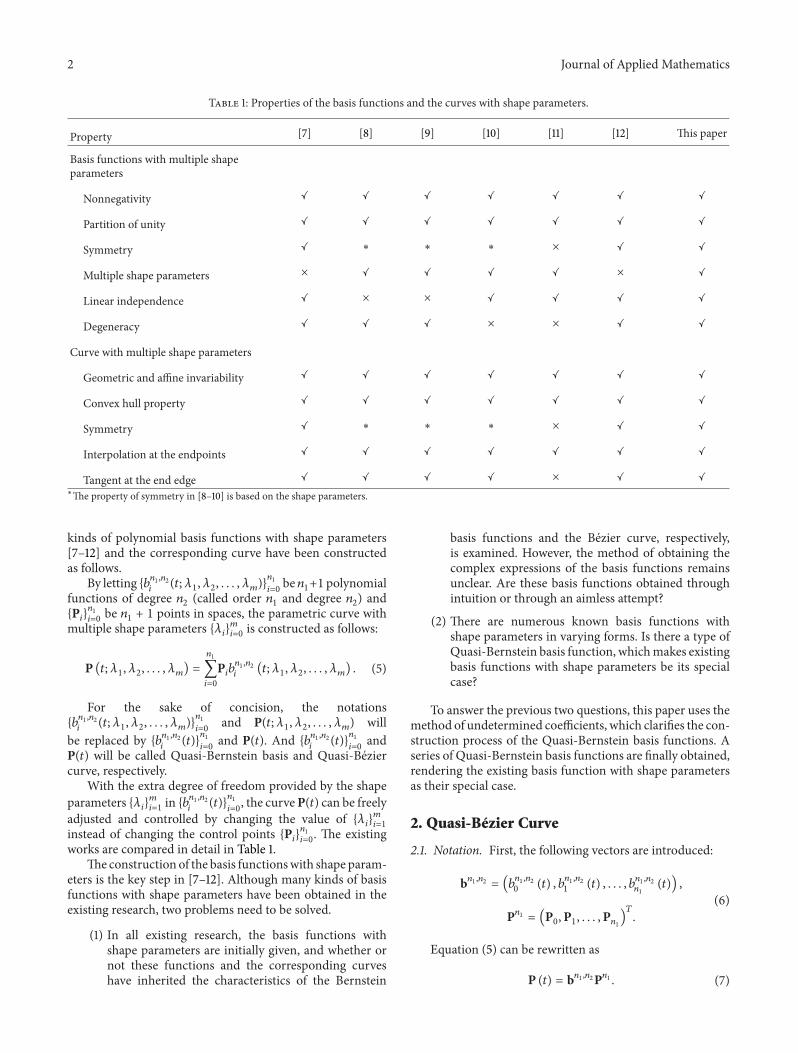
Table 1 Properties of the basis functions and the curves with shape parameters
Property [7] [8] [9] [10] [11] [12] This paper
Basis functions with multiple shapeparameters
Nonnegativity
Partition of unity
Symmetry lowast lowast lowast times
Multiple shape parameters times times
Linear independence times times
Degeneracy times times
Curve with multiple shape parameters
Geometric and affine invariability
Convex hull property
Symmetry lowast lowast lowast times
Interpolation at the endpoints
Tangent at the end edge times
lowastThe property of symmetry in [8ndash10] is based on the shape parameters
kinds of polynomial basis functions with shape parameters[7ndash12] and the corresponding curve have been constructedas follows
By letting 1198871198991 1198992119894
(119905 1205821 1205822 120582
119898)1198991
119894=0be 1198991+1 polynomial
functions of degree 1198992(called order 119899
1and degree 119899
2) and
P1198941198991
119894=0be 1198991+ 1 points in spaces the parametric curve with
multiple shape parameters 120582119894119898
119894=0is constructed as follows
P (119905 1205821 1205822 120582
119898) =
1198991
sum
119894=0
P11989411988711989911198992
119894(119905 1205821 1205822 120582
119898) (5)
For the sake of concision the notations11988711989911198992
119894(119905 1205821 1205822 120582
119898)1198991
119894=0and P(119905 120582
1 1205822 120582
119898) will
be replaced by 11988711989911198992
119894(119905)1198991
119894=0and P(119905) And 119887
11989911198992
119894(119905)1198991
119894=0and
P(119905) will be called Quasi-Bernstein basis and Quasi-Beziercurve respectively
With the extra degree of freedom provided by the shapeparameters 120582
119894119898
119894=1in 11988711989911198992
119894(119905)1198991
119894=0 the curveP(119905) can be freely
adjusted and controlled by changing the value of 120582119894119898
119894=1
instead of changing the control points P1198941198991
119894=0 The existing
works are compared in detail in Table 1The construction of the basis functionswith shape param-
eters is the key step in [7ndash12] Although many kinds of basisfunctions with shape parameters have been obtained in theexisting research two problems need to be solved
(1) In all existing research the basis functions withshape parameters are initially given and whether ornot these functions and the corresponding curveshave inherited the characteristics of the Bernstein
basis functions and the Bezier curve respectivelyis examined However the method of obtaining thecomplex expressions of the basis functions remainsunclear Are these basis functions obtained throughintuition or through an aimless attempt
(2) There are numerous known basis functions withshape parameters in varying forms Is there a type ofQuasi-Bernstein basis function whichmakes existingbasis functions with shape parameters be its specialcase
To answer the previous two questions this paper uses themethod of undetermined coefficients which clarifies the con-struction process of the Quasi-Bernstein basis functions Aseries of Quasi-Bernstein basis functions are finally obtainedrendering the existing basis function with shape parametersas their special case
2 Quasi-Beacutezier Curve
21 Notation First the following vectors are introduced
b11989911198992 = (11988711989911198992
0(119905) 11988711989911198992
1(119905) 119887
11989911198992
1198991
(119905))
P1198991 = (P0P1 P
1198991
)119879
(6)
Equation (5) can be rewritten as
P (119905) = b1198991 1198992P1198991 (7)
Journal of Applied Mathematics 3
Given that 1198871198991 1198992119894
(119905)1198991
119894=0are polynomials with degree 119899
2
they can be seen as the linear combination of the Bernsteinbasis functions 1198611198992
119894(119905)1198992
119894=0with degree 119899
2given by
b1198991 1198992 = B1198992M1198992 1198991
B1198992 = (1198611198992
0(119905) 1198611198992
1(119905) 119861
1198992
1198992
(119905))
M1198992 1198991 = (119898119894119895)119894=1198992119895=1198991
119894119895=0
(8)
Thus as long as the elements in the matrix M1198992 1198991 aredetermined the Quasi-Bernstein basis functions 11988711989911198992
119894(119905)1198991
119894=0
with order 1198991and degree 119899
2are completely constructed
Except for several elements that can be determined inM1198992 1198991 the rest are shape parameters of the Quasi-Bernstein basisfunctions and theQuasi-Bezier curve Here thematrixM11989921198991is called the shape parameter matrix
22 Construction of the Shape Parameter Matrix M1198992 1198991 The(1198992+1)(119899
1+1) elements of119898
119894119895inM11989921198991 must be determined so
that 1198871198991 1198992119894
(119905)1198991
119894=0and P(119905) become the Quasi-Bernstein basis
functions and the Quasi-Bezier curve respectively
221 Determination of 119898119894119895according to the Characteristics
of the Quasi-Bernstein Basis Functions The Quasi-Bernsteinbasis functions 1198871198991 1198992
119894(119905)1198991
119894=0with order 119899
1and degree 119899
2must
satisfy the characteristics of nonnegativity normalizationsymmetry linear independence and degeneracy
Proposition 1 (nonnegativity) A sufficient condition for11988711989911198992
119894(119905) ge 0 (119894 = 0 1 119899
2) is
119898119894119895ge 0 (119894 = 0 1 119899
2 119895 = 0 1 119899
1) (9)
Proof Here 11988711989911198992
119895(119905) = sum
1198992
119894=01198981198941198951198611198992
119894(119905) is known to have
been extracted from (8) Based on the non-negativity of theBernstein basis functions 119861
1198992
119894(119905)1198992
119894=0 a sufficient condition
for the non-negativity of the Quasi-Bernstein basis functions11988711989911198992
119894(119905)1198991
119894=0is the non-negativity of the elements 119898
119894119895in
M1198992 1198991 Hence119898119894119895must satisfy (9)
Note 1 Clearly there is no row with all elements being 0 inM1198992 1198991 In other words
1198992
sum
119894=0
119898119894119895
= 0 (119895 = 0 1 1198991) (10)
Proposition 2 (normalization) The necessary and sufficientcondition for sum1198991
119895=011988711989911198992
119895(119905) = 1 is given by
1198991
sum
119895=0
119898119894119895= 1 (119894 = 0 1 119899
2) (11)
Proof It is known that
1198991
sum
119895=0
11988711989911198992
119895(119905) minus 1
=
1198991
sum
119895=0
(
1198992
sum
119894=0
1198981198941198951198611198992
119894(119905)) minus 1
=
1198992
sum
119894=0
(
1198991
sum
119895=0
119898119894119895)1198611198992
119894(119905) minus 1
=
1198992
sum
119894=0
(
1198991
sum
119895=0
119898119894119895)1198611198992
119894(119905) minus
1198992
sum
119894=0
1198611198992
119894(119905)
=
1198992
sum
119894=0
(
1198991
sum
119895=0
119898119894119895minus 1)119861
1198992
119894(119905)
(12)
According to the linear independence of the Bernsteinbasis functions 119861
1198992
119894(119905)1198992
119894=0 the necessary and sufficient con-
dition for sum1198991
119895=011988711989911198992
119895(119905) minus 1 = 0 is sum
1198991
119895=0119898119894119895
= 1 (119894 =
0 1 1198992)
Note 2 By combining (9) and (11) 119898119894119895satisfies 0 le 119898
119894119895le
1 (119894 = 0 1 1198992 119895 = 0 1 119899
1)
Proposition 3 (symmetry) The necessary and sufficient con-dition for 1198871198991 1198992
119895(119905) = 119887
11989911198992
1198991minus119895
(1 minus 119905) (119895 = 0 1 1198991) is given by
119898119894119895= 1198981198992minus1198941198991minus119895
(119894 = 0 1 1198992 119895 = 0 1 119899
1) (13)
Proof According to the symmetry of the Bernstein basisfunctions 119861
1198992
119894(119905)1198992
119894=0of 1198611198992119894(119905) = 119861
1198992
1198992minus119894(1 minus 119905) the following
can be derived
11988711989911198992
1198991minus119895
(1 minus 119905) minus 11988711989911198992
119895(119905)
=
1198992
sum
119894=0
1198611198992
119894(1 minus 119905)119898
1198941198991minus119895
minus
1198992
sum
119894=0
1198611198992
119894(119905)119898119894119895
=
1198992
sum
119894=0
1198611198992
1198992minus119894(119905)1198981198941198991minus119895
minus
1198992
sum
119894=0
1198611198992
119894(119905)119898119894119895
=
1198992
sum
119894=0
1198611198992
119894(119905)1198981198992minus1198941198991minus119895
minus
1198992
sum
119894=0
1198611198992
119894(119905)119898119894119895
=
1198992
sum
119894=0
1198611198992
119894(119905) (119898
1198992minus1198941198991minus119895
minus 119898119894119895)
119895 = 0 1 1198991
(14)
According to the linear independence of the Bernsteinbasis functions 119861
1198992
119894(119905)1198992
119894=0 the necessary and sufficient con-
dition for 1198871198991 1198992119895
(119905) minus 11988711989911198992
1198991minus119895
(1 minus 119905) = 0 is (13)
4 Journal of Applied Mathematics
Proposition 4 (linear independence) The necessary andsufficient condition for the linear independence of 11988711989911198992
119894(119905)1198991
119894=0
is given by
119903 (M1198992 1198991) = 1198991+ 1 (15)
Proof It is known that
1198991
sum
119895=0
11989611989511988711989911198992
119895(119905) =
1198991
sum
119895=0
119896119895(
1198992
sum
119894=0
1198981198941198951198611198992
119894(119905))
=
1198992
sum
119894=0
(
1198991
sum
119895=0
119896119895119898119894119895)1198611198992
119894(119905)
(16)
According to the linear independence of the Bernsteinbasis functions 119861
1198992
119894(119905)1198992
119894=0 the necessary and sufficient con-
dition for sum1198991119895=0
11989611989511988711989911198992
119895(119905) = 0 is given by
1198991
sum
119895=0
119896119895119898119894119895= 0 (119894 = 0 1 119899
2) (17)
M119895 = (1198980119895
1198981119895
1198981198992119895)119879 is defined as the 119895th column
vector ofM11989921198991 Equation (17) is equivalent tosum1198991
119895=0119896119895M119895 = 0
Thus the necessary and sufficient condition for the linearindependence of 1198871198991 1198992
119894(119905)1198991
119894=0is also the linear independence
of the column vectors M1198951198991119894=0
of the matrix M1198992 1198991 Conse-quently the necessary and sufficient condition for the linearindependence of 119887
11989911198992
119894(119905)1198991
119894=0is that the rank of the shape
parameter matrixM1198992 1198991 satisfies 119903(M11989921198991) = 1198991+ 1
Note 3 When (15) is true 1198992ge 1198991
Proposition 5 (degeneracy) If the elements 119898119894119895119894=1198992119895=1198991
119894119895=0in
the matrixM1198992 1198991 are represented by (18) the Quasi-Bernsteinbasis functions 119887
11989911198992
119894(119905)1198991
119894=0with order 119899
1and degree 119899
2are
degenerated into the Bernstein basis functions 1198611198991119894(119905)1198991
119894=0with
order 1198991
119898119894119895
=
(1198992minus1198991
119894minus119895) (1198991
119895 )
(1198992
119894)
max (0 119894 minus (1198992minus 1198991)) le 119895 le min (119899
1 119894)
0 le 119894 le 1198992 0 le 119895 le 119899
1
0 else(18)
Proof When the elements 119898119894119895119894=1198992119895=1198991
119894119895=0in the matrix M11989921198991
are represented by (18) the following is obtained
B1198991 = B1198992M11989921198991 (19)
Comparing (19) with (8) Proposition 5 is proven
Note 4 If 1198991= 1198992M1198992 1198991 is an identity matrix here
222 Determination of 119898119894119895according to the Characteristics of
the Quasi-Bezier Curve
Proposition6 (interpolation at the endpoints) Thenecessaryand sufficient condition for P(0) = P
0and P(1) = P
1198991
is givenby
11989800
= 1 1198980119895
= 0 (119895 = 1 2 1198991) (20)
11989811989921198991
= 1 1198981198992119895= 0 (119895 = 0 1 119899
1minus 1) (21)
Proof Clearly the necessary and sufficient condition forP(0) = P
0is the Quasi-Bernstein primary functions
11988711989911198992
119894(119905)1198991
119894=0satisfying the following
11988711989911198992
119894(0) =
1 119894 = 0
0 119894 = 0(22)
It is known that
(11988711989911198992
0(0) 11988711989911198992
1(0) 119887
11989911198992
1198991
(0))
= (1198611198992
0(0) 119861
1198992
1(0) 119861
1198992
1198992
(0)) sdot (119898119894119895)119894=1198992119895=1198991
119894119895=0
= (1 0 0) sdot (119898119894119895)119894=1198992119895=1198991
119894119895=0
= (11989800 11989801 119898
01198991minus1 11989801198991
)
(23)
Thus the necessary and sufficient condition for (1198871198991 11989920
(0)11988711989911198992
1(0) 119887
11989911198992
1198991
(0)) = (1 0 0) is (20)Similarly the necessary and sufficient condition for
P(1) = P1198991
is the Quasi-Bernstein primary functions11988711989911198992
119894(119905)1198991
119894=0satisfying the following
11988711989911198992
119894(1) =
1 119894 = 1198991
0 119894 = 1198991
(24)
It is known that
(11988711989911198992
0(1) 11988711989911198992
1(1) 119887
11989911198992
1198991
(1))
= (1198611198992
0(1) 119861
1198992
1(1) 119861
1198992
1198992
(1)) sdot (119898119894119895)119894=1198992119895=1198991
119894119895=0
= (0 0 1) sdot (119898119894119895)119894=1198992119895=1198991
119894119895=0
= (11989811989920 11989811989921 119898
11989921198991minus1 11989811989921198991
)
(25)
Thus the necessary and sufficient condition for(11988711989911198992
0(1) 11988711989911198992
1(1) 119887
11989911198992
1198991
(1)) = (0 0 1) is (21)Hence the necessary and sufficient condition for P(1) =
P1198991
is (21)
Note 5 When 11988711989911198992
119894(119905)1198991
119894=0have the property of symmetry
(21) is equivalent to (20) according to (13)
Journal of Applied Mathematics 5
Proposition 7 (tangent edges at the endpoints) The neces-sary and sufficient condition for P1015840(0)P
1P0P1015840(1)P
119899P119899minus1
isgiven by
11989810
+ 11989811
= 1 11989810
= 1
1198981119895
= 0 (119895 = 2 3 1198991)
(26)
1198981198992minus11198991minus1
+ 1198981198992minus11198991
= 1 1198981198992minus11198991
= 1
1198981198992minus1119895
= 0 (119895 = 0 1 1198991minus 2)
(27)
Proof It is known that
P1015840 (0) = P1015840 (119905)10038161003816100381610038161003816119905=0
= (11988711989911198992
0(119905) 11988711989911198992
1(119905) 119887
11989911198992
1198991
(119905))1015840100381610038161003816100381610038161003816119905=0
times (P0P1 P
1198991
)119879
= (1198611198992
0(119905) 1198611198992
1(119905) 119861
1198992
1198992
(119905))1015840100381610038161003816100381610038161003816119905=0
sdot (119898119894119895)119894=1198992119895=1198991
119894119895=0
sdot (P0P1 P
1198991
)119879
= 1198992(minus1 1 0 0) sdot (119898
119894119895)119894=1198992119895=1198991
119894119895=0sdot (P0P1 P
1198991
)119879
= 1198992(11989810
minus 11989800 11989811
minus 11989801 119898
11198991
minus 11989801198991
)
times (P0P1 P
1198991
)119879
(28)
Clearly the necessary and sufficient condition forP1015840(0)P
1P0is (11989810
minus 11989800)(11989811
minus 11989801) = minus1 119898
1119895minus 1198980119895
=
0 (119895 = 2 3 1198991) which verifies (26)
Similarly the necessary and sufficient condition forP1015840(1)P
119899P119899minus1
is (27)
Note 6 When 11988711989911198992
119894(119905)1198991
119894=0have the property of symmetry
(27) is equivalent to (26) according to (13)
223 Form of Shape Parameter Matrix M11989921198991 All shapeparameter matrixes that satisfy (9) (11) (13) (15) (20) (21)(26) and (27) have the following form
M1198992 1198991 =((((
(
1 0 sdot sdot sdot 0 0
11989810
1 minus 11989810
sdot sdot sdot 0 0
11989820
11989821
sdot sdot sdot 11989821198991minus1
11989821198991
11989821198991
11989821198991minus1
sdot sdot sdot 11989821
11989820
0 0 sdot sdot sdot 1 minus 11989810
11989810
0 0 sdot sdot sdot 0 1
))))
)(1198992+1)times(119899
1+1)
(29)
Here119898119894119895are variable shape parameters that satisfy
1198991
sum
119895=0
119898119894119895= 1 (119894 = 2 3 [
(1198992+ 1)
2]) 0 le 119898
10lt 1
0 le 119898119894119895le 1(119894 = 2 3 [
(1198992+ 1)
2] 119895 = 0 1 119899
1)
(30)
23 The Characteristics of the Quasi-Bezier Curve In sum-mary the Quasi-Bezier curve P(119905) based on the Quasi-Bernstein basis functions 1198871198991 1198992
119894(119905)1198991
119894=0has the characteristics
listed as follows
(a) shape adjustability the shape of the Quasi-Beziercurve can still be adjusted by maintaining the controlpoints
(b) geometric invariability the Quasi-Bezier curve onlyrelies on the control points whereas it has nothing todo with the position and direction of the coordinatesystem in other words the curve shape remainsinvariable after translation and revolving in the coor-dinate system
(c) affine invariability barycentric combinations areinvariant under affine maps therefore (9) and (11)give the algebraic verification of this property
(d) symmetry whether the control points are labeledP0P1sdot sdot sdotP1198991
or P1198991
P1198991minus1
sdot sdot sdotP0 the curves that corre-
spond to the two different orderings look the samethey differ only in the direction in which they aretraversed and this is written as1198991
sum
119894=0
P11989411988711989911198992
119894(119905) =
1198991
sum
119894=0
P1198991minus11989411988711989911198992
1198991minus119894
(1 minus 119905) (31)
which follows the inspection of (13)(e) convex hull property this property exists since the
Quasi-Bernstein basis functions 1198871198991 1198992119894
(119905)1198991
119894=0have the
properties of non-negativity and normalization theQuasi-Bezier curve is the convex linear combinationof control points and as such it is located in theconvex hull of the control points
(f) interpolation at the endpoints and tangent edges atthe endpoint the Quasi-Bezier curve P(119905) interpo-lates the first and the last control points P(0) =
P0and P(1) = P
1198991
the first and last edges of thecontrol polygon are the tangent lines at the endpointswhere P1015840(0)P
1P0and P1015840(1)P
119899P119899minus1
24 Geometric Significance of the Shape Parameters Accord-ing to (29) when 119898
1198941198950
(119894 = 0 1 1198992 1198950
= 0 1 1198991)
increases 1198871198991 11989921198950
(119905) and 11988711989911198992
1198991minus1198950
(119905) increase as well specificallyP(119905) comes close to the control points P
1198950
and P1198991minus1198950
Thegeometric significance of the shape parameters is shown inSection 3
6 Journal of Applied Mathematics
0 02 04 06 08 10
02
04
06
08
1
11989810 = 0
11989810 = 04
11989810 = 08
(a)
0 1 2 3 4 50
02
04
06
08
1
11989810 = 0
11989810 = 04
11989810 = 08
Bezier curve
1199271
11992721199270
(b)
Figure 1 Quasi-Bernstein basis functions and Quasi-Bezier curves when 1198991= 2 and 119899
2= 3
3 Numerical Examples
Example 1 The shape parameter matrix M32 is constructedfrom (29) The corresponding Quasi-Bernstein basis func-tions and the Quasi-Bezier curves with different shapeparameter119898
10are given as follows
M32 = (
1 0 0
11989810
1 minus 11989810
0
0 1 minus 11989810
11989810
0 0 1
) 0 le 11989810
lt 1 (32)
The geometric significance of the shape parameters 11989810
is shown in Figure 1 As the value of the shape parameter11989810
increases the elements in the second column of M32decrease According to (8) the second Quasi-Bernstein basisfunction 119887
23
1(119905) decreases So the corresponding Quasi-
Bezier curve moves away from the control point P1(see
Figure 1(b))
Example 2 The shape parameter matrix M42 is constructedfrom (29) The corresponding Quasi-Bernstein basis func-tions and the Quasi-Bezier curves with different shapeparameters119898
10and119898
20are given as follows
M42 = (
1 0 0
11989810
1 minus 11989810
0
11989820
1 minus 211989820
11989820
0 1 minus 11989810
11989810
0 0 1
)
0 le 11989810
lt 1 0 le 11989820
le1
2
(33)
The geometric significance of the shape parameters 11989810
and 11989820
is shown in Figure 2 When we increase the valueof 11989810and keep 119898
20unchanged the elements in the second
column ofM42 decrease According to (8) the secondQuasi-Bernstein basis function 119887
24
1(119905) decreases Compare the blue
curve with the red one and we will find that the Quasi-Beziercurvemoves away from the control pointP
1(see Figure 2(b))
If we increase the value of 11989820and keep 119898
10unchanged
similar result is also obtained Compare the red curve withthe green one and we will find that the Quasi-Bezier curvemoves away from the control point P
1(see Figure 2(b))
Example 3 The shape parameter matrix M33 is constructedfrom (29) The corresponding Quasi-Bernstein basis func-tions and the Quasi-Bezier curves with different shapeparameter119898
10are given as follows
M33 = (
1 0 0 0
11989810
1 minus 11989810
0 0
0 0 1 minus 11989810
11989810
0 0 0 1
) 0 le 11989810
lt 1
(34)
The geometric significance of the shape parameters11989810is
shown in Figure 3 As the value of the shape parameter 11989810
increases the elements in the second and the third column ofM33 decrease According to (8) the second Quasi-Bernsteinbasis function 119887
33
1(119905) and the third Quasi-Bernstein basis
function 11988733
2(119905) decrease So the corresponding Quasi-Bezier
curve moves away from the control points P1and P
2(see
Figure 3(b))
Example 4 The shape parameter matrix M43 is construc-ted from (29) The corresponding Quasi-Bernstein basis
Journal of Applied Mathematics 7
0 02 04 06 08 10
02
04
06
08
1
11989810 = 011989820 = 011989810 = 0611989820 = 0
11989810 = 0611989820 = 03
(a)
11989810 = 011989820 = 011989810 = 0611989820 = 011989810 = 0611989820 = 03
Bezier curve
0 21 3 4 50
02
04
06
08
11199271
11992721199270
(b)
Figure 2 Quasi-Bernstein basis functions and Quasi-Bezier curves when 1198991= 2 and 119899
2= 4
11989810 = 02
11989810 = 05
11989810 = 08
0 02 04 06 08 10
02
04
06
08
1
(a)
0 1 2 3 4 50
1
05
15
2
25
3
11989810 = 02
11989810 = 05
11989810 = 08
Bezier curve
1199271
1199272
1199270
1199273
(b)
Figure 3 Quasi-Bernstein basis functions and Quasi-Bezier curves when 1198991= 3 and 119899
2= 3
functions and the Quasi-Bezier curves with different shapeparameter119898
10and119898
20are given as follows
M43 =(((
(
1 0 0 0
11989810
1 minus 11989810
0 0
11989820
1
2minus 11989820
1
2minus 11989820
11989820
0 0 1 minus 11989810
11989810
0 0 0 1
)))
)
0 le 11989810
lt 1 0 le 11989820
le1
2
(35)
The geometric significance of the shape parameters 11989810
and 11989820
is shown in Figure 4 When we increase the valueof 11989810and keep 119898
20unchanged the elements in the second
and the third column ofM43 decrease According to (8) thesecond Quasi-Bernstein basis function 119887
34
1(119905) and the third
Quasi-Bernstein basis function 11988734
2(119905) decrease Compare the
blue curve with the red one and we will find that the Quasi-Bezier curve moves away from the control points P
1and P
2
(see Figure 4(b))If we increase the value of 119898
20and keep 119898
10unchanged
similar result is also obtained Compare the red curvewith thegreen one andwewill find that theQuasi-Bezier curvemovesaway from the control points P
1and P
2(see Figure 4(b))
8 Journal of Applied Mathematics
0 02 04 06 08 10
02
04
06
08
1
11989810 = 011989820 = 011989810 = 0611989820 = 0
11989810 = 0611989820 = 03
(a)
0 1 2 3 4 50
1
05
15
2
25
3
11989810 = 011989820 = 011989810 = 0611989820 = 011989810 = 0611989820 = 03
Bezier curve
1199271
1199272
11992701199273
(b)
Figure 4 Quasi-Bernstein basis functions and Quasi-Bezier curves when 1198991= 3 and 119899
2= 4
Figure 5 Three kinds of flowers with six petals
Note 7 Several Quasi-Bernstein basis functions for lowdegree and low order are presented aforementioned Thecorresponding basis functions for higher degree and higherorder are defined recursively as follows [7 12]
1198871198991+11198992+1
119894(119905) = (1 minus 119905) 119887
11989911198992
119894(119905) + 119905119887
11989911198992
119894minus1(119905)
119894 = 0 1 1198991
(36)
Here we set 11988711989911198992minus1
(119905) = 11988711989911198992
1198991+1
(119905) = 0
Example 5 Figure 5 presents three kinds of flowers with sixpetals defined by six symmetric control polygons Similarflowers are obtained from the same control polygons withdifferent shape parameters
Example 6 Figure 6 presents three kinds of outlines of thevase all of which are similar to the control polygons So the
Figure 6 Three kinds of outlines of the vase
designer canmakeminute adjustments with the same controlpolygons by changing the value of the shape parameters
4 Discussion
41 Special Cases Several existing basis functions containingjust one shape parameter in [7 12] are considered as thespecial cases in this paper Meanwhile for the polynomialbasis functions with multiple shape parameters in [8ndash11] thesymmetry was not discussed by authors In fact when theseshape parameters satisfy certain relations the correspondingbasis functions and curves become symmetrical Then thecurves have geometric and affine invariability convex hullproperty symmetry interpolation at the endpoints and
Journal of Applied Mathematics 9
tangent edges at the endpoints and the corresponding shapeparameter matrices are the special cases of (29)
We take [9] as example When the shape parameterssatisfy certain relations in [9] the shape parameter matrix is
M119899+1119899
=
((((((((((((((((((
(
1 0 sdot sdot sdot 0 0
1 minus 1205821
119899 + 11 minus
1 minus 1205821
119899 + 1sdot sdot sdot 0 0
02 minus 1205822
119899 + 1sdot sdot sdot 0 0
0 0 sdot sdot sdot
2 minus 1205822
119899 + 10
0 0 sdot sdot sdot 1 minus1 minus 1205821
119899 + 1
1 minus 1205821
119899 + 1
0 0 sdot sdot sdot 0 1
))))))))))))))))))
)(119899+2)times(119899+1)
(37)
It is the special case of (29)
42 Degree and Order of the Curve In the previous work thedifference between the degree and order of the curve is fixed(ie 119899
2minus1198991= 0 in [10 11] 119899
2minus1198991= 1 in [7ndash9] and 119899
2minus1198991= 2
in [12]) and the scope of the curve is also fixed with the samecontrol points
However comparing Figures 1(a) and 1(b) it is found thatthe greater the difference between degree and order the largerthe scope of the Quasi-Bezier curve acquired In order toobtain the Quasi-Bezier curves with broader scope with thesame control points the designer can increase the differencebetween the degree and the order 119899
2minus 1198991
5 Conclusion and Further Work
In this paper a series of univariate Quasi-Bernstein basisfunctions are constructed thereby creating a series of Quasi-Bezier curves The shape of the series of curves can beadjusted even with the control points fixedThe Quasi-Beziercurves also possess geometric and affine invariability convexhull property symmetry interpolation at the endpoints andtangent edges at the endpoints
Quasi-Bernstein basis functions with shape parametershave been directly studied in the previous research Howeverin this paper each function has been gradually inferred andconstructed using a clear method of undetermined coeffi-cients where each shape parameter is proposed accordingto the properties of the Quasi-Bernstein basis functions andthe Quasi-Bezier curve Under the premise of satisfyingsymmetry the former basis functions are all considered as thespecial cases in this paper
In the existing CADCAM systems the triangular Beziersurface and the spline curve are widely used The shapeparameters also have been brought into the triangular surfacein [12ndash14] and the spline curve [15ndash17] The method in thispaper also can be extended to construct the basis functionsof the triangular surface and the spline curve with shape
parameters directly andmore details can be seen in our otherpapers submitted
Acknowledgments
The author is very grateful to the anonymous refereesfor the inspiring comments and the valuable suggestionswhich improved the paper considerably This work has beensupported by the National Natural Science Foundation ofChina (no Y5090377) and the Natural Science Foundationof Ningbo (nos 2011A610174 and 2012A610029)
References
[1] G Farin ldquoAlgorithms for rational Bezier curvesrdquo Computer-Aided Design vol 15 no 2 pp 73ndash77 1983
[2] I Juhasz ldquoWeight-based shapemodification of NURBS curvesrdquoComputer Aided Geometric Design vol 16 no 5 pp 377ndash3831999
[3] L Piegl ldquoModifying the shape of rational B-splines Part 1curvesrdquoComputer-AidedDesign vol 21 no 8 pp 509ndash518 1989
[4] Q Chen and GWang ldquoA class of Bezier-like curvesrdquo ComputerAided Geometric Design vol 20 no 1 pp 29ndash39 2003
[5] J Zhang ldquoC-curves an extension of cubic curvesrdquo ComputerAided Geometric Design vol 13 no 3 pp 199ndash217 1996
[6] J Zhang F L Krause and H Zhang ldquoUnifying C-curves andH-curves by extending the calculation to complex numbersrdquoComputer Aided Geometric Design vol 22 no 9 pp 865ndash8832005
[7] X Wu ldquoBezier curve with shape parameterrdquo Journal of Imageand Graphics vol 11 pp 369ndash374 2006
[8] X A Han Y Ma and X Huang ldquoA novel generalization ofBezier curve and surfacerdquo Journal of Computational andAppliedMathematics vol 217 no 1 pp 180ndash193 2008
[9] L Yang and X M Zeng ldquoBezier curves and surfaces with shapeparametersrdquo International Journal of Computer Mathematicsvol 86 no 7 pp 1253ndash1263 2009
[10] T Xiang Z Liu W Wang and P Jiang ldquoA novel extensionof Bezier curves and surfaces of the same degreerdquo Journal ofInformation amp Computational Science vol 7 pp 2080ndash20892010
[11] J Chen and G-j Wang ldquoA new type of the generalized Beziercurvesrdquo Applied Mathematics vol 26 no 1 pp 47ndash56 2011
[12] L Yan and J Liang ldquoAn extension of the Bezier modelrdquo AppliedMathematics and Computation vol 218 no 6 pp 2863ndash28792011
[13] J Cao and G Wang ldquoAn extension of Bernstein-Bezier surfaceover the triangular domainrdquo Progress in Natural Science vol 17no 3 pp 352ndash357 2007
[14] Z Liu J Tan and X Chen ldquoCubic Bezier triangular patchwith shape parametersrdquo Journal of Computer Research andDevelopment vol 49 pp 152ndash157 2012
[15] X Han ldquoQuadratic trigonometric polynomial curves with ashape parameterrdquoComputer AidedGeometric Design vol 19 no7 pp 503ndash512 2002
[16] X Han ldquoCubic trigonometric polynomial curves with a shapeparameterrdquoComputer Aided Geometric Design vol 21 no 6 pp535ndash548 2004
[17] X Han ldquoA class of general quartic spline curves with shapeparametersrdquo Computer Aided Geometric Design vol 28 no 3pp 151ndash163 2011
Submit your manuscripts athttpwwwhindawicom
Hindawi Publishing Corporationhttpwwwhindawicom Volume 2014
MathematicsJournal of
Hindawi Publishing Corporationhttpwwwhindawicom Volume 2014
Mathematical Problems in Engineering
Hindawi Publishing Corporationhttpwwwhindawicom
Differential EquationsInternational Journal of
Volume 2014
Applied MathematicsJournal of
Hindawi Publishing Corporationhttpwwwhindawicom Volume 2014
Probability and StatisticsHindawi Publishing Corporationhttpwwwhindawicom Volume 2014
Journal of
Hindawi Publishing Corporationhttpwwwhindawicom Volume 2014
Mathematical PhysicsAdvances in
Complex AnalysisJournal of
Hindawi Publishing Corporationhttpwwwhindawicom Volume 2014
OptimizationJournal of
Hindawi Publishing Corporationhttpwwwhindawicom Volume 2014
CombinatoricsHindawi Publishing Corporationhttpwwwhindawicom Volume 2014
International Journal of
Hindawi Publishing Corporationhttpwwwhindawicom Volume 2014
Operations ResearchAdvances in
Journal of
Hindawi Publishing Corporationhttpwwwhindawicom Volume 2014
Function Spaces
Abstract and Applied AnalysisHindawi Publishing Corporationhttpwwwhindawicom Volume 2014
International Journal of Mathematics and Mathematical Sciences
Hindawi Publishing Corporationhttpwwwhindawicom Volume 2014
The Scientific World JournalHindawi Publishing Corporation httpwwwhindawicom Volume 2014
Hindawi Publishing Corporationhttpwwwhindawicom Volume 2014
Algebra
Discrete Dynamics in Nature and Society
Hindawi Publishing Corporationhttpwwwhindawicom Volume 2014
Hindawi Publishing Corporationhttpwwwhindawicom Volume 2014
Decision SciencesAdvances in
Discrete MathematicsJournal of
Hindawi Publishing Corporationhttpwwwhindawicom
Volume 2014
Hindawi Publishing Corporationhttpwwwhindawicom Volume 2014
Stochastic AnalysisInternational Journal of
2 Journal of Applied Mathematics
Table 1 Properties of the basis functions and the curves with shape parameters
Property [7] [8] [9] [10] [11] [12] This paper
Basis functions with multiple shapeparameters
Nonnegativity
Partition of unity
Symmetry lowast lowast lowast times
Multiple shape parameters times times
Linear independence times times
Degeneracy times times
Curve with multiple shape parameters
Geometric and affine invariability
Convex hull property
Symmetry lowast lowast lowast times
Interpolation at the endpoints
Tangent at the end edge times
lowastThe property of symmetry in [8ndash10] is based on the shape parameters
kinds of polynomial basis functions with shape parameters[7ndash12] and the corresponding curve have been constructedas follows
By letting 1198871198991 1198992119894
(119905 1205821 1205822 120582
119898)1198991
119894=0be 1198991+1 polynomial
functions of degree 1198992(called order 119899
1and degree 119899
2) and
P1198941198991
119894=0be 1198991+ 1 points in spaces the parametric curve with
multiple shape parameters 120582119894119898
119894=0is constructed as follows
P (119905 1205821 1205822 120582
119898) =
1198991
sum
119894=0
P11989411988711989911198992
119894(119905 1205821 1205822 120582
119898) (5)
For the sake of concision the notations11988711989911198992
119894(119905 1205821 1205822 120582
119898)1198991
119894=0and P(119905 120582
1 1205822 120582
119898) will
be replaced by 11988711989911198992
119894(119905)1198991
119894=0and P(119905) And 119887
11989911198992
119894(119905)1198991
119894=0and
P(119905) will be called Quasi-Bernstein basis and Quasi-Beziercurve respectively
With the extra degree of freedom provided by the shapeparameters 120582
119894119898
119894=1in 11988711989911198992
119894(119905)1198991
119894=0 the curveP(119905) can be freely
adjusted and controlled by changing the value of 120582119894119898
119894=1
instead of changing the control points P1198941198991
119894=0 The existing
works are compared in detail in Table 1The construction of the basis functionswith shape param-
eters is the key step in [7ndash12] Although many kinds of basisfunctions with shape parameters have been obtained in theexisting research two problems need to be solved
(1) In all existing research the basis functions withshape parameters are initially given and whether ornot these functions and the corresponding curveshave inherited the characteristics of the Bernstein
basis functions and the Bezier curve respectivelyis examined However the method of obtaining thecomplex expressions of the basis functions remainsunclear Are these basis functions obtained throughintuition or through an aimless attempt
(2) There are numerous known basis functions withshape parameters in varying forms Is there a type ofQuasi-Bernstein basis function whichmakes existingbasis functions with shape parameters be its specialcase
To answer the previous two questions this paper uses themethod of undetermined coefficients which clarifies the con-struction process of the Quasi-Bernstein basis functions Aseries of Quasi-Bernstein basis functions are finally obtainedrendering the existing basis function with shape parametersas their special case
2 Quasi-Beacutezier Curve
21 Notation First the following vectors are introduced
b11989911198992 = (11988711989911198992
0(119905) 11988711989911198992
1(119905) 119887
11989911198992
1198991
(119905))
P1198991 = (P0P1 P
1198991
)119879
(6)
Equation (5) can be rewritten as
P (119905) = b1198991 1198992P1198991 (7)
Journal of Applied Mathematics 3
Given that 1198871198991 1198992119894
(119905)1198991
119894=0are polynomials with degree 119899
2
they can be seen as the linear combination of the Bernsteinbasis functions 1198611198992
119894(119905)1198992
119894=0with degree 119899
2given by
b1198991 1198992 = B1198992M1198992 1198991
B1198992 = (1198611198992
0(119905) 1198611198992
1(119905) 119861
1198992
1198992
(119905))
M1198992 1198991 = (119898119894119895)119894=1198992119895=1198991
119894119895=0
(8)
Thus as long as the elements in the matrix M1198992 1198991 aredetermined the Quasi-Bernstein basis functions 11988711989911198992
119894(119905)1198991
119894=0
with order 1198991and degree 119899
2are completely constructed
Except for several elements that can be determined inM1198992 1198991 the rest are shape parameters of the Quasi-Bernstein basisfunctions and theQuasi-Bezier curve Here thematrixM11989921198991is called the shape parameter matrix
22 Construction of the Shape Parameter Matrix M1198992 1198991 The(1198992+1)(119899
1+1) elements of119898
119894119895inM11989921198991 must be determined so
that 1198871198991 1198992119894
(119905)1198991
119894=0and P(119905) become the Quasi-Bernstein basis
functions and the Quasi-Bezier curve respectively
221 Determination of 119898119894119895according to the Characteristics
of the Quasi-Bernstein Basis Functions The Quasi-Bernsteinbasis functions 1198871198991 1198992
119894(119905)1198991
119894=0with order 119899
1and degree 119899
2must
satisfy the characteristics of nonnegativity normalizationsymmetry linear independence and degeneracy
Proposition 1 (nonnegativity) A sufficient condition for11988711989911198992
119894(119905) ge 0 (119894 = 0 1 119899
2) is
119898119894119895ge 0 (119894 = 0 1 119899
2 119895 = 0 1 119899
1) (9)
Proof Here 11988711989911198992
119895(119905) = sum
1198992
119894=01198981198941198951198611198992
119894(119905) is known to have
been extracted from (8) Based on the non-negativity of theBernstein basis functions 119861
1198992
119894(119905)1198992
119894=0 a sufficient condition
for the non-negativity of the Quasi-Bernstein basis functions11988711989911198992
119894(119905)1198991
119894=0is the non-negativity of the elements 119898
119894119895in
M1198992 1198991 Hence119898119894119895must satisfy (9)
Note 1 Clearly there is no row with all elements being 0 inM1198992 1198991 In other words
1198992
sum
119894=0
119898119894119895
= 0 (119895 = 0 1 1198991) (10)
Proposition 2 (normalization) The necessary and sufficientcondition for sum1198991
119895=011988711989911198992
119895(119905) = 1 is given by
1198991
sum
119895=0
119898119894119895= 1 (119894 = 0 1 119899
2) (11)
Proof It is known that
1198991
sum
119895=0
11988711989911198992
119895(119905) minus 1
=
1198991
sum
119895=0
(
1198992
sum
119894=0
1198981198941198951198611198992
119894(119905)) minus 1
=
1198992
sum
119894=0
(
1198991
sum
119895=0
119898119894119895)1198611198992
119894(119905) minus 1
=
1198992
sum
119894=0
(
1198991
sum
119895=0
119898119894119895)1198611198992
119894(119905) minus
1198992
sum
119894=0
1198611198992
119894(119905)
=
1198992
sum
119894=0
(
1198991
sum
119895=0
119898119894119895minus 1)119861
1198992
119894(119905)
(12)
According to the linear independence of the Bernsteinbasis functions 119861
1198992
119894(119905)1198992
119894=0 the necessary and sufficient con-
dition for sum1198991
119895=011988711989911198992
119895(119905) minus 1 = 0 is sum
1198991
119895=0119898119894119895
= 1 (119894 =
0 1 1198992)
Note 2 By combining (9) and (11) 119898119894119895satisfies 0 le 119898
119894119895le
1 (119894 = 0 1 1198992 119895 = 0 1 119899
1)
Proposition 3 (symmetry) The necessary and sufficient con-dition for 1198871198991 1198992
119895(119905) = 119887
11989911198992
1198991minus119895
(1 minus 119905) (119895 = 0 1 1198991) is given by
119898119894119895= 1198981198992minus1198941198991minus119895
(119894 = 0 1 1198992 119895 = 0 1 119899
1) (13)
Proof According to the symmetry of the Bernstein basisfunctions 119861
1198992
119894(119905)1198992
119894=0of 1198611198992119894(119905) = 119861
1198992
1198992minus119894(1 minus 119905) the following
can be derived
11988711989911198992
1198991minus119895
(1 minus 119905) minus 11988711989911198992
119895(119905)
=
1198992
sum
119894=0
1198611198992
119894(1 minus 119905)119898
1198941198991minus119895
minus
1198992
sum
119894=0
1198611198992
119894(119905)119898119894119895
=
1198992
sum
119894=0
1198611198992
1198992minus119894(119905)1198981198941198991minus119895
minus
1198992
sum
119894=0
1198611198992
119894(119905)119898119894119895
=
1198992
sum
119894=0
1198611198992
119894(119905)1198981198992minus1198941198991minus119895
minus
1198992
sum
119894=0
1198611198992
119894(119905)119898119894119895
=
1198992
sum
119894=0
1198611198992
119894(119905) (119898
1198992minus1198941198991minus119895
minus 119898119894119895)
119895 = 0 1 1198991
(14)
According to the linear independence of the Bernsteinbasis functions 119861
1198992
119894(119905)1198992
119894=0 the necessary and sufficient con-
dition for 1198871198991 1198992119895
(119905) minus 11988711989911198992
1198991minus119895
(1 minus 119905) = 0 is (13)
4 Journal of Applied Mathematics
Proposition 4 (linear independence) The necessary andsufficient condition for the linear independence of 11988711989911198992
119894(119905)1198991
119894=0
is given by
119903 (M1198992 1198991) = 1198991+ 1 (15)
Proof It is known that
1198991
sum
119895=0
11989611989511988711989911198992
119895(119905) =
1198991
sum
119895=0
119896119895(
1198992
sum
119894=0
1198981198941198951198611198992
119894(119905))
=
1198992
sum
119894=0
(
1198991
sum
119895=0
119896119895119898119894119895)1198611198992
119894(119905)
(16)
According to the linear independence of the Bernsteinbasis functions 119861
1198992
119894(119905)1198992
119894=0 the necessary and sufficient con-
dition for sum1198991119895=0
11989611989511988711989911198992
119895(119905) = 0 is given by
1198991
sum
119895=0
119896119895119898119894119895= 0 (119894 = 0 1 119899
2) (17)
M119895 = (1198980119895
1198981119895
1198981198992119895)119879 is defined as the 119895th column
vector ofM11989921198991 Equation (17) is equivalent tosum1198991
119895=0119896119895M119895 = 0
Thus the necessary and sufficient condition for the linearindependence of 1198871198991 1198992
119894(119905)1198991
119894=0is also the linear independence
of the column vectors M1198951198991119894=0
of the matrix M1198992 1198991 Conse-quently the necessary and sufficient condition for the linearindependence of 119887
11989911198992
119894(119905)1198991
119894=0is that the rank of the shape
parameter matrixM1198992 1198991 satisfies 119903(M11989921198991) = 1198991+ 1
Note 3 When (15) is true 1198992ge 1198991
Proposition 5 (degeneracy) If the elements 119898119894119895119894=1198992119895=1198991
119894119895=0in
the matrixM1198992 1198991 are represented by (18) the Quasi-Bernsteinbasis functions 119887
11989911198992
119894(119905)1198991
119894=0with order 119899
1and degree 119899
2are
degenerated into the Bernstein basis functions 1198611198991119894(119905)1198991
119894=0with
order 1198991
119898119894119895
=
(1198992minus1198991
119894minus119895) (1198991
119895 )
(1198992
119894)
max (0 119894 minus (1198992minus 1198991)) le 119895 le min (119899
1 119894)
0 le 119894 le 1198992 0 le 119895 le 119899
1
0 else(18)
Proof When the elements 119898119894119895119894=1198992119895=1198991
119894119895=0in the matrix M11989921198991
are represented by (18) the following is obtained
B1198991 = B1198992M11989921198991 (19)
Comparing (19) with (8) Proposition 5 is proven
Note 4 If 1198991= 1198992M1198992 1198991 is an identity matrix here
222 Determination of 119898119894119895according to the Characteristics of
the Quasi-Bezier Curve
Proposition6 (interpolation at the endpoints) Thenecessaryand sufficient condition for P(0) = P
0and P(1) = P
1198991
is givenby
11989800
= 1 1198980119895
= 0 (119895 = 1 2 1198991) (20)
11989811989921198991
= 1 1198981198992119895= 0 (119895 = 0 1 119899
1minus 1) (21)
Proof Clearly the necessary and sufficient condition forP(0) = P
0is the Quasi-Bernstein primary functions
11988711989911198992
119894(119905)1198991
119894=0satisfying the following
11988711989911198992
119894(0) =
1 119894 = 0
0 119894 = 0(22)
It is known that
(11988711989911198992
0(0) 11988711989911198992
1(0) 119887
11989911198992
1198991
(0))
= (1198611198992
0(0) 119861
1198992
1(0) 119861
1198992
1198992
(0)) sdot (119898119894119895)119894=1198992119895=1198991
119894119895=0
= (1 0 0) sdot (119898119894119895)119894=1198992119895=1198991
119894119895=0
= (11989800 11989801 119898
01198991minus1 11989801198991
)
(23)
Thus the necessary and sufficient condition for (1198871198991 11989920
(0)11988711989911198992
1(0) 119887
11989911198992
1198991
(0)) = (1 0 0) is (20)Similarly the necessary and sufficient condition for
P(1) = P1198991
is the Quasi-Bernstein primary functions11988711989911198992
119894(119905)1198991
119894=0satisfying the following
11988711989911198992
119894(1) =
1 119894 = 1198991
0 119894 = 1198991
(24)
It is known that
(11988711989911198992
0(1) 11988711989911198992
1(1) 119887
11989911198992
1198991
(1))
= (1198611198992
0(1) 119861
1198992
1(1) 119861
1198992
1198992
(1)) sdot (119898119894119895)119894=1198992119895=1198991
119894119895=0
= (0 0 1) sdot (119898119894119895)119894=1198992119895=1198991
119894119895=0
= (11989811989920 11989811989921 119898
11989921198991minus1 11989811989921198991
)
(25)
Thus the necessary and sufficient condition for(11988711989911198992
0(1) 11988711989911198992
1(1) 119887
11989911198992
1198991
(1)) = (0 0 1) is (21)Hence the necessary and sufficient condition for P(1) =
P1198991
is (21)
Note 5 When 11988711989911198992
119894(119905)1198991
119894=0have the property of symmetry
(21) is equivalent to (20) according to (13)
Journal of Applied Mathematics 5
Proposition 7 (tangent edges at the endpoints) The neces-sary and sufficient condition for P1015840(0)P
1P0P1015840(1)P
119899P119899minus1
isgiven by
11989810
+ 11989811
= 1 11989810
= 1
1198981119895
= 0 (119895 = 2 3 1198991)
(26)
1198981198992minus11198991minus1
+ 1198981198992minus11198991
= 1 1198981198992minus11198991
= 1
1198981198992minus1119895
= 0 (119895 = 0 1 1198991minus 2)
(27)
Proof It is known that
P1015840 (0) = P1015840 (119905)10038161003816100381610038161003816119905=0
= (11988711989911198992
0(119905) 11988711989911198992
1(119905) 119887
11989911198992
1198991
(119905))1015840100381610038161003816100381610038161003816119905=0
times (P0P1 P
1198991
)119879
= (1198611198992
0(119905) 1198611198992
1(119905) 119861
1198992
1198992
(119905))1015840100381610038161003816100381610038161003816119905=0
sdot (119898119894119895)119894=1198992119895=1198991
119894119895=0
sdot (P0P1 P
1198991
)119879
= 1198992(minus1 1 0 0) sdot (119898
119894119895)119894=1198992119895=1198991
119894119895=0sdot (P0P1 P
1198991
)119879
= 1198992(11989810
minus 11989800 11989811
minus 11989801 119898
11198991
minus 11989801198991
)
times (P0P1 P
1198991
)119879
(28)
Clearly the necessary and sufficient condition forP1015840(0)P
1P0is (11989810
minus 11989800)(11989811
minus 11989801) = minus1 119898
1119895minus 1198980119895
=
0 (119895 = 2 3 1198991) which verifies (26)
Similarly the necessary and sufficient condition forP1015840(1)P
119899P119899minus1
is (27)
Note 6 When 11988711989911198992
119894(119905)1198991
119894=0have the property of symmetry
(27) is equivalent to (26) according to (13)
223 Form of Shape Parameter Matrix M11989921198991 All shapeparameter matrixes that satisfy (9) (11) (13) (15) (20) (21)(26) and (27) have the following form
M1198992 1198991 =((((
(
1 0 sdot sdot sdot 0 0
11989810
1 minus 11989810
sdot sdot sdot 0 0
11989820
11989821
sdot sdot sdot 11989821198991minus1
11989821198991
11989821198991
11989821198991minus1
sdot sdot sdot 11989821
11989820
0 0 sdot sdot sdot 1 minus 11989810
11989810
0 0 sdot sdot sdot 0 1
))))
)(1198992+1)times(119899
1+1)
(29)
Here119898119894119895are variable shape parameters that satisfy
1198991
sum
119895=0
119898119894119895= 1 (119894 = 2 3 [
(1198992+ 1)
2]) 0 le 119898
10lt 1
0 le 119898119894119895le 1(119894 = 2 3 [
(1198992+ 1)
2] 119895 = 0 1 119899
1)
(30)
23 The Characteristics of the Quasi-Bezier Curve In sum-mary the Quasi-Bezier curve P(119905) based on the Quasi-Bernstein basis functions 1198871198991 1198992
119894(119905)1198991
119894=0has the characteristics
listed as follows
(a) shape adjustability the shape of the Quasi-Beziercurve can still be adjusted by maintaining the controlpoints
(b) geometric invariability the Quasi-Bezier curve onlyrelies on the control points whereas it has nothing todo with the position and direction of the coordinatesystem in other words the curve shape remainsinvariable after translation and revolving in the coor-dinate system
(c) affine invariability barycentric combinations areinvariant under affine maps therefore (9) and (11)give the algebraic verification of this property
(d) symmetry whether the control points are labeledP0P1sdot sdot sdotP1198991
or P1198991
P1198991minus1
sdot sdot sdotP0 the curves that corre-
spond to the two different orderings look the samethey differ only in the direction in which they aretraversed and this is written as1198991
sum
119894=0
P11989411988711989911198992
119894(119905) =
1198991
sum
119894=0
P1198991minus11989411988711989911198992
1198991minus119894
(1 minus 119905) (31)
which follows the inspection of (13)(e) convex hull property this property exists since the
Quasi-Bernstein basis functions 1198871198991 1198992119894
(119905)1198991
119894=0have the
properties of non-negativity and normalization theQuasi-Bezier curve is the convex linear combinationof control points and as such it is located in theconvex hull of the control points
(f) interpolation at the endpoints and tangent edges atthe endpoint the Quasi-Bezier curve P(119905) interpo-lates the first and the last control points P(0) =
P0and P(1) = P
1198991
the first and last edges of thecontrol polygon are the tangent lines at the endpointswhere P1015840(0)P
1P0and P1015840(1)P
119899P119899minus1
24 Geometric Significance of the Shape Parameters Accord-ing to (29) when 119898
1198941198950
(119894 = 0 1 1198992 1198950
= 0 1 1198991)
increases 1198871198991 11989921198950
(119905) and 11988711989911198992
1198991minus1198950
(119905) increase as well specificallyP(119905) comes close to the control points P
1198950
and P1198991minus1198950
Thegeometric significance of the shape parameters is shown inSection 3
6 Journal of Applied Mathematics
0 02 04 06 08 10
02
04
06
08
1
11989810 = 0
11989810 = 04
11989810 = 08
(a)
0 1 2 3 4 50
02
04
06
08
1
11989810 = 0
11989810 = 04
11989810 = 08
Bezier curve
1199271
11992721199270
(b)
Figure 1 Quasi-Bernstein basis functions and Quasi-Bezier curves when 1198991= 2 and 119899
2= 3
3 Numerical Examples
Example 1 The shape parameter matrix M32 is constructedfrom (29) The corresponding Quasi-Bernstein basis func-tions and the Quasi-Bezier curves with different shapeparameter119898
10are given as follows
M32 = (
1 0 0
11989810
1 minus 11989810
0
0 1 minus 11989810
11989810
0 0 1
) 0 le 11989810
lt 1 (32)
The geometric significance of the shape parameters 11989810
is shown in Figure 1 As the value of the shape parameter11989810
increases the elements in the second column of M32decrease According to (8) the second Quasi-Bernstein basisfunction 119887
23
1(119905) decreases So the corresponding Quasi-
Bezier curve moves away from the control point P1(see
Figure 1(b))
Example 2 The shape parameter matrix M42 is constructedfrom (29) The corresponding Quasi-Bernstein basis func-tions and the Quasi-Bezier curves with different shapeparameters119898
10and119898
20are given as follows
M42 = (
1 0 0
11989810
1 minus 11989810
0
11989820
1 minus 211989820
11989820
0 1 minus 11989810
11989810
0 0 1
)
0 le 11989810
lt 1 0 le 11989820
le1
2
(33)
The geometric significance of the shape parameters 11989810
and 11989820
is shown in Figure 2 When we increase the valueof 11989810and keep 119898
20unchanged the elements in the second
column ofM42 decrease According to (8) the secondQuasi-Bernstein basis function 119887
24
1(119905) decreases Compare the blue
curve with the red one and we will find that the Quasi-Beziercurvemoves away from the control pointP
1(see Figure 2(b))
If we increase the value of 11989820and keep 119898
10unchanged
similar result is also obtained Compare the red curve withthe green one and we will find that the Quasi-Bezier curvemoves away from the control point P
1(see Figure 2(b))
Example 3 The shape parameter matrix M33 is constructedfrom (29) The corresponding Quasi-Bernstein basis func-tions and the Quasi-Bezier curves with different shapeparameter119898
10are given as follows
M33 = (
1 0 0 0
11989810
1 minus 11989810
0 0
0 0 1 minus 11989810
11989810
0 0 0 1
) 0 le 11989810
lt 1
(34)
The geometric significance of the shape parameters11989810is
shown in Figure 3 As the value of the shape parameter 11989810
increases the elements in the second and the third column ofM33 decrease According to (8) the second Quasi-Bernsteinbasis function 119887
33
1(119905) and the third Quasi-Bernstein basis
function 11988733
2(119905) decrease So the corresponding Quasi-Bezier
curve moves away from the control points P1and P
2(see
Figure 3(b))
Example 4 The shape parameter matrix M43 is construc-ted from (29) The corresponding Quasi-Bernstein basis
Journal of Applied Mathematics 7
0 02 04 06 08 10
02
04
06
08
1
11989810 = 011989820 = 011989810 = 0611989820 = 0
11989810 = 0611989820 = 03
(a)
11989810 = 011989820 = 011989810 = 0611989820 = 011989810 = 0611989820 = 03
Bezier curve
0 21 3 4 50
02
04
06
08
11199271
11992721199270
(b)
Figure 2 Quasi-Bernstein basis functions and Quasi-Bezier curves when 1198991= 2 and 119899
2= 4
11989810 = 02
11989810 = 05
11989810 = 08
0 02 04 06 08 10
02
04
06
08
1
(a)
0 1 2 3 4 50
1
05
15
2
25
3
11989810 = 02
11989810 = 05
11989810 = 08
Bezier curve
1199271
1199272
1199270
1199273
(b)
Figure 3 Quasi-Bernstein basis functions and Quasi-Bezier curves when 1198991= 3 and 119899
2= 3
functions and the Quasi-Bezier curves with different shapeparameter119898
10and119898
20are given as follows
M43 =(((
(
1 0 0 0
11989810
1 minus 11989810
0 0
11989820
1
2minus 11989820
1
2minus 11989820
11989820
0 0 1 minus 11989810
11989810
0 0 0 1
)))
)
0 le 11989810
lt 1 0 le 11989820
le1
2
(35)
The geometric significance of the shape parameters 11989810
and 11989820
is shown in Figure 4 When we increase the valueof 11989810and keep 119898
20unchanged the elements in the second
and the third column ofM43 decrease According to (8) thesecond Quasi-Bernstein basis function 119887
34
1(119905) and the third
Quasi-Bernstein basis function 11988734
2(119905) decrease Compare the
blue curve with the red one and we will find that the Quasi-Bezier curve moves away from the control points P
1and P
2
(see Figure 4(b))If we increase the value of 119898
20and keep 119898
10unchanged
similar result is also obtained Compare the red curvewith thegreen one andwewill find that theQuasi-Bezier curvemovesaway from the control points P
1and P
2(see Figure 4(b))
8 Journal of Applied Mathematics
0 02 04 06 08 10
02
04
06
08
1
11989810 = 011989820 = 011989810 = 0611989820 = 0
11989810 = 0611989820 = 03
(a)
0 1 2 3 4 50
1
05
15
2
25
3
11989810 = 011989820 = 011989810 = 0611989820 = 011989810 = 0611989820 = 03
Bezier curve
1199271
1199272
11992701199273
(b)
Figure 4 Quasi-Bernstein basis functions and Quasi-Bezier curves when 1198991= 3 and 119899
2= 4
Figure 5 Three kinds of flowers with six petals
Note 7 Several Quasi-Bernstein basis functions for lowdegree and low order are presented aforementioned Thecorresponding basis functions for higher degree and higherorder are defined recursively as follows [7 12]
1198871198991+11198992+1
119894(119905) = (1 minus 119905) 119887
11989911198992
119894(119905) + 119905119887
11989911198992
119894minus1(119905)
119894 = 0 1 1198991
(36)
Here we set 11988711989911198992minus1
(119905) = 11988711989911198992
1198991+1
(119905) = 0
Example 5 Figure 5 presents three kinds of flowers with sixpetals defined by six symmetric control polygons Similarflowers are obtained from the same control polygons withdifferent shape parameters
Example 6 Figure 6 presents three kinds of outlines of thevase all of which are similar to the control polygons So the
Figure 6 Three kinds of outlines of the vase
designer canmakeminute adjustments with the same controlpolygons by changing the value of the shape parameters
4 Discussion
41 Special Cases Several existing basis functions containingjust one shape parameter in [7 12] are considered as thespecial cases in this paper Meanwhile for the polynomialbasis functions with multiple shape parameters in [8ndash11] thesymmetry was not discussed by authors In fact when theseshape parameters satisfy certain relations the correspondingbasis functions and curves become symmetrical Then thecurves have geometric and affine invariability convex hullproperty symmetry interpolation at the endpoints and
Journal of Applied Mathematics 9
tangent edges at the endpoints and the corresponding shapeparameter matrices are the special cases of (29)
We take [9] as example When the shape parameterssatisfy certain relations in [9] the shape parameter matrix is
M119899+1119899
=
((((((((((((((((((
(
1 0 sdot sdot sdot 0 0
1 minus 1205821
119899 + 11 minus
1 minus 1205821
119899 + 1sdot sdot sdot 0 0
02 minus 1205822
119899 + 1sdot sdot sdot 0 0
0 0 sdot sdot sdot
2 minus 1205822
119899 + 10
0 0 sdot sdot sdot 1 minus1 minus 1205821
119899 + 1
1 minus 1205821
119899 + 1
0 0 sdot sdot sdot 0 1
))))))))))))))))))
)(119899+2)times(119899+1)
(37)
It is the special case of (29)
42 Degree and Order of the Curve In the previous work thedifference between the degree and order of the curve is fixed(ie 119899
2minus1198991= 0 in [10 11] 119899
2minus1198991= 1 in [7ndash9] and 119899
2minus1198991= 2
in [12]) and the scope of the curve is also fixed with the samecontrol points
However comparing Figures 1(a) and 1(b) it is found thatthe greater the difference between degree and order the largerthe scope of the Quasi-Bezier curve acquired In order toobtain the Quasi-Bezier curves with broader scope with thesame control points the designer can increase the differencebetween the degree and the order 119899
2minus 1198991
5 Conclusion and Further Work
In this paper a series of univariate Quasi-Bernstein basisfunctions are constructed thereby creating a series of Quasi-Bezier curves The shape of the series of curves can beadjusted even with the control points fixedThe Quasi-Beziercurves also possess geometric and affine invariability convexhull property symmetry interpolation at the endpoints andtangent edges at the endpoints
Quasi-Bernstein basis functions with shape parametershave been directly studied in the previous research Howeverin this paper each function has been gradually inferred andconstructed using a clear method of undetermined coeffi-cients where each shape parameter is proposed accordingto the properties of the Quasi-Bernstein basis functions andthe Quasi-Bezier curve Under the premise of satisfyingsymmetry the former basis functions are all considered as thespecial cases in this paper
In the existing CADCAM systems the triangular Beziersurface and the spline curve are widely used The shapeparameters also have been brought into the triangular surfacein [12ndash14] and the spline curve [15ndash17] The method in thispaper also can be extended to construct the basis functionsof the triangular surface and the spline curve with shape
parameters directly andmore details can be seen in our otherpapers submitted
Acknowledgments
The author is very grateful to the anonymous refereesfor the inspiring comments and the valuable suggestionswhich improved the paper considerably This work has beensupported by the National Natural Science Foundation ofChina (no Y5090377) and the Natural Science Foundationof Ningbo (nos 2011A610174 and 2012A610029)
References
[1] G Farin ldquoAlgorithms for rational Bezier curvesrdquo Computer-Aided Design vol 15 no 2 pp 73ndash77 1983
[2] I Juhasz ldquoWeight-based shapemodification of NURBS curvesrdquoComputer Aided Geometric Design vol 16 no 5 pp 377ndash3831999
[3] L Piegl ldquoModifying the shape of rational B-splines Part 1curvesrdquoComputer-AidedDesign vol 21 no 8 pp 509ndash518 1989
[4] Q Chen and GWang ldquoA class of Bezier-like curvesrdquo ComputerAided Geometric Design vol 20 no 1 pp 29ndash39 2003
[5] J Zhang ldquoC-curves an extension of cubic curvesrdquo ComputerAided Geometric Design vol 13 no 3 pp 199ndash217 1996
[6] J Zhang F L Krause and H Zhang ldquoUnifying C-curves andH-curves by extending the calculation to complex numbersrdquoComputer Aided Geometric Design vol 22 no 9 pp 865ndash8832005
[7] X Wu ldquoBezier curve with shape parameterrdquo Journal of Imageand Graphics vol 11 pp 369ndash374 2006
[8] X A Han Y Ma and X Huang ldquoA novel generalization ofBezier curve and surfacerdquo Journal of Computational andAppliedMathematics vol 217 no 1 pp 180ndash193 2008
[9] L Yang and X M Zeng ldquoBezier curves and surfaces with shapeparametersrdquo International Journal of Computer Mathematicsvol 86 no 7 pp 1253ndash1263 2009
[10] T Xiang Z Liu W Wang and P Jiang ldquoA novel extensionof Bezier curves and surfaces of the same degreerdquo Journal ofInformation amp Computational Science vol 7 pp 2080ndash20892010
[11] J Chen and G-j Wang ldquoA new type of the generalized Beziercurvesrdquo Applied Mathematics vol 26 no 1 pp 47ndash56 2011
[12] L Yan and J Liang ldquoAn extension of the Bezier modelrdquo AppliedMathematics and Computation vol 218 no 6 pp 2863ndash28792011
[13] J Cao and G Wang ldquoAn extension of Bernstein-Bezier surfaceover the triangular domainrdquo Progress in Natural Science vol 17no 3 pp 352ndash357 2007
[14] Z Liu J Tan and X Chen ldquoCubic Bezier triangular patchwith shape parametersrdquo Journal of Computer Research andDevelopment vol 49 pp 152ndash157 2012
[15] X Han ldquoQuadratic trigonometric polynomial curves with ashape parameterrdquoComputer AidedGeometric Design vol 19 no7 pp 503ndash512 2002
[16] X Han ldquoCubic trigonometric polynomial curves with a shapeparameterrdquoComputer Aided Geometric Design vol 21 no 6 pp535ndash548 2004
[17] X Han ldquoA class of general quartic spline curves with shapeparametersrdquo Computer Aided Geometric Design vol 28 no 3pp 151ndash163 2011
Submit your manuscripts athttpwwwhindawicom
Hindawi Publishing Corporationhttpwwwhindawicom Volume 2014
MathematicsJournal of
Hindawi Publishing Corporationhttpwwwhindawicom Volume 2014
Mathematical Problems in Engineering
Hindawi Publishing Corporationhttpwwwhindawicom
Differential EquationsInternational Journal of
Volume 2014
Applied MathematicsJournal of
Hindawi Publishing Corporationhttpwwwhindawicom Volume 2014
Probability and StatisticsHindawi Publishing Corporationhttpwwwhindawicom Volume 2014
Journal of
Hindawi Publishing Corporationhttpwwwhindawicom Volume 2014
Mathematical PhysicsAdvances in
Complex AnalysisJournal of
Hindawi Publishing Corporationhttpwwwhindawicom Volume 2014
OptimizationJournal of
Hindawi Publishing Corporationhttpwwwhindawicom Volume 2014
CombinatoricsHindawi Publishing Corporationhttpwwwhindawicom Volume 2014
International Journal of
Hindawi Publishing Corporationhttpwwwhindawicom Volume 2014
Operations ResearchAdvances in
Journal of
Hindawi Publishing Corporationhttpwwwhindawicom Volume 2014
Function Spaces
Abstract and Applied AnalysisHindawi Publishing Corporationhttpwwwhindawicom Volume 2014
International Journal of Mathematics and Mathematical Sciences
Hindawi Publishing Corporationhttpwwwhindawicom Volume 2014
The Scientific World JournalHindawi Publishing Corporation httpwwwhindawicom Volume 2014
Hindawi Publishing Corporationhttpwwwhindawicom Volume 2014
Algebra
Discrete Dynamics in Nature and Society
Hindawi Publishing Corporationhttpwwwhindawicom Volume 2014
Hindawi Publishing Corporationhttpwwwhindawicom Volume 2014
Decision SciencesAdvances in
Discrete MathematicsJournal of
Hindawi Publishing Corporationhttpwwwhindawicom
Volume 2014
Hindawi Publishing Corporationhttpwwwhindawicom Volume 2014
Stochastic AnalysisInternational Journal of
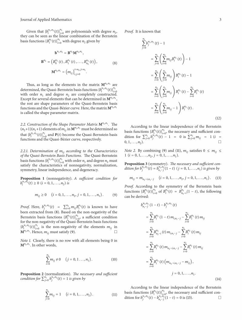
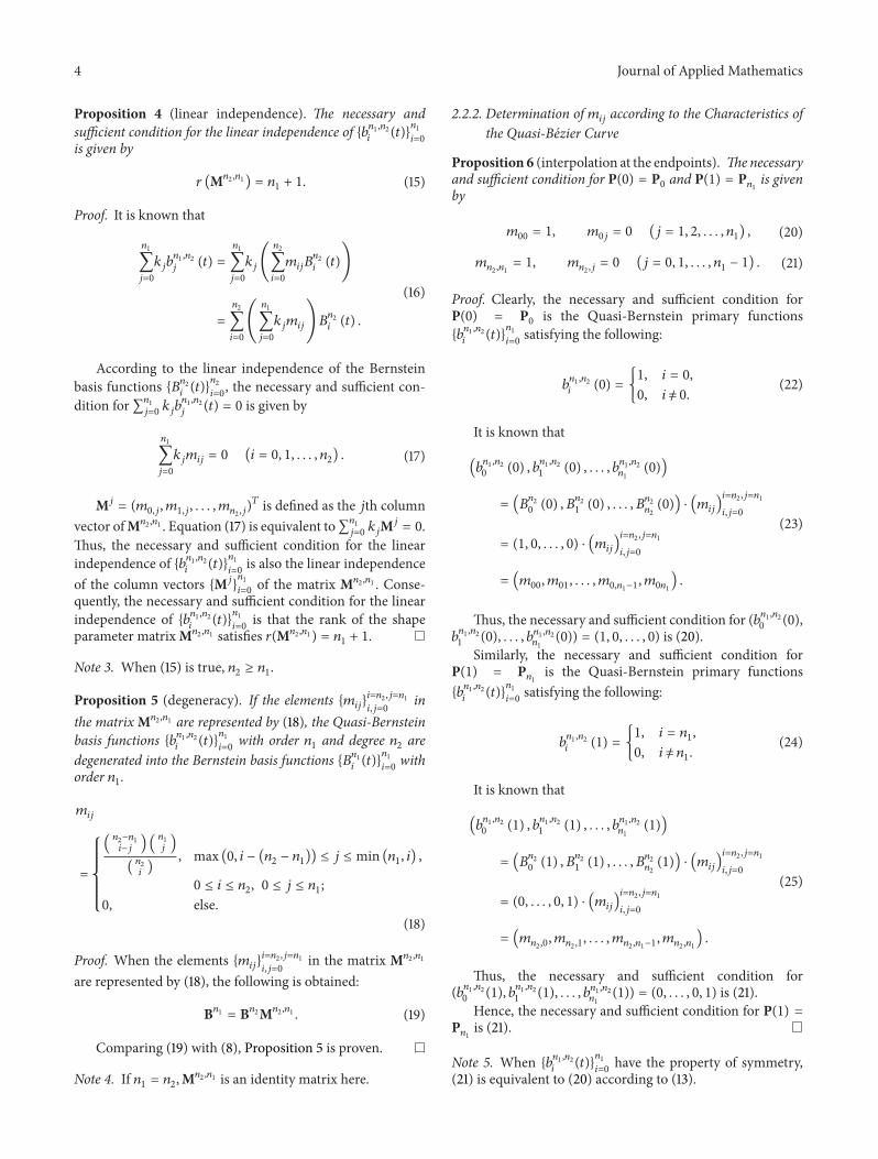
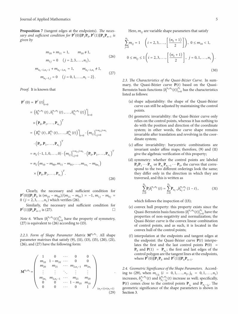
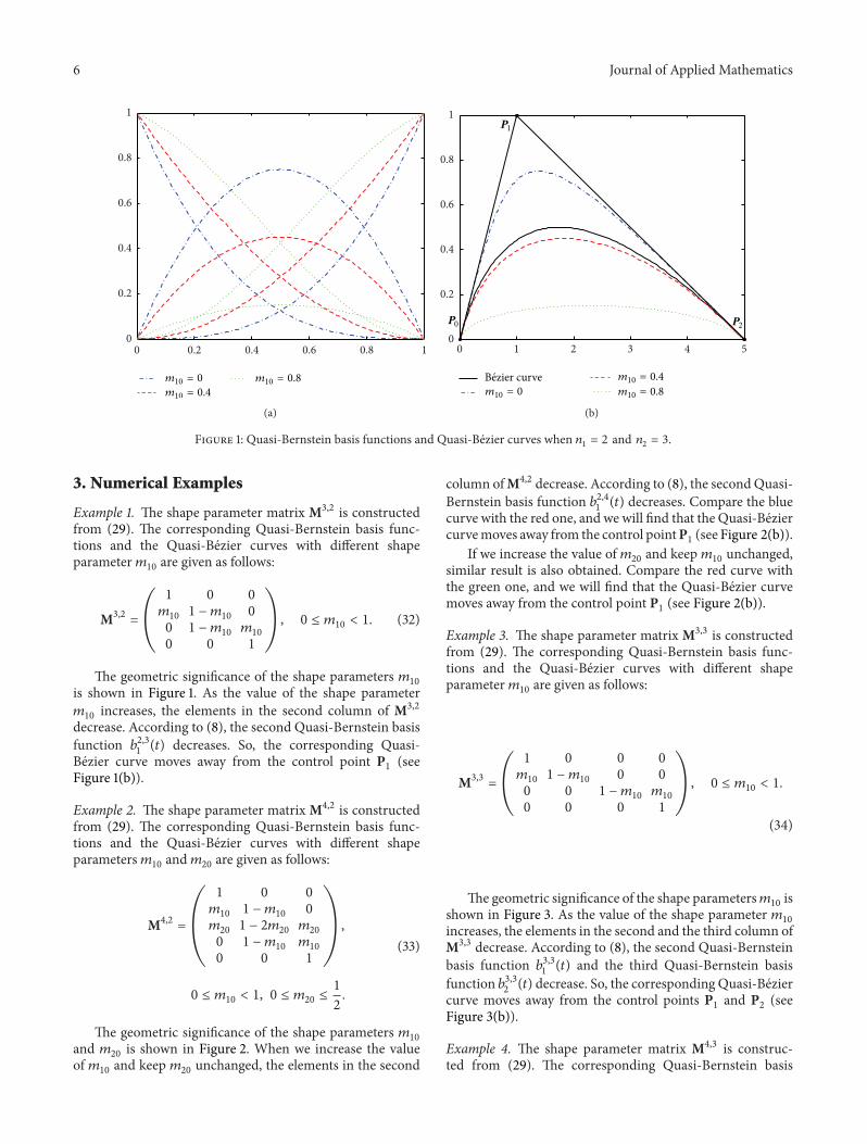
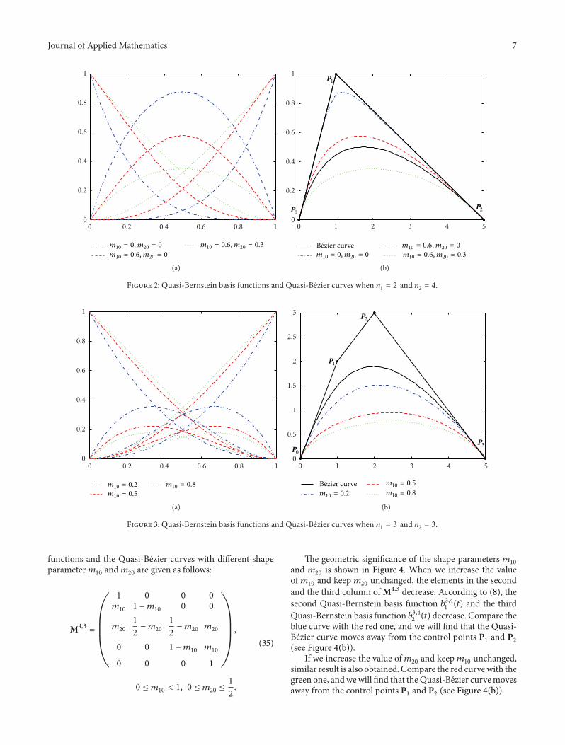
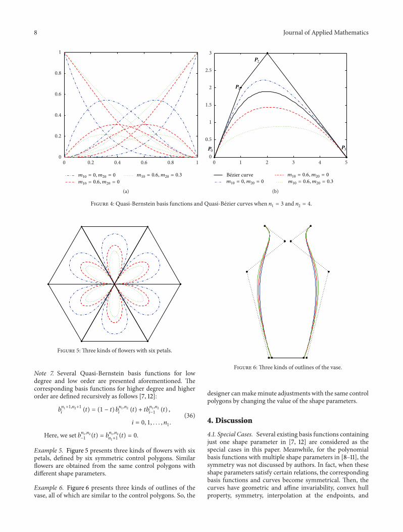
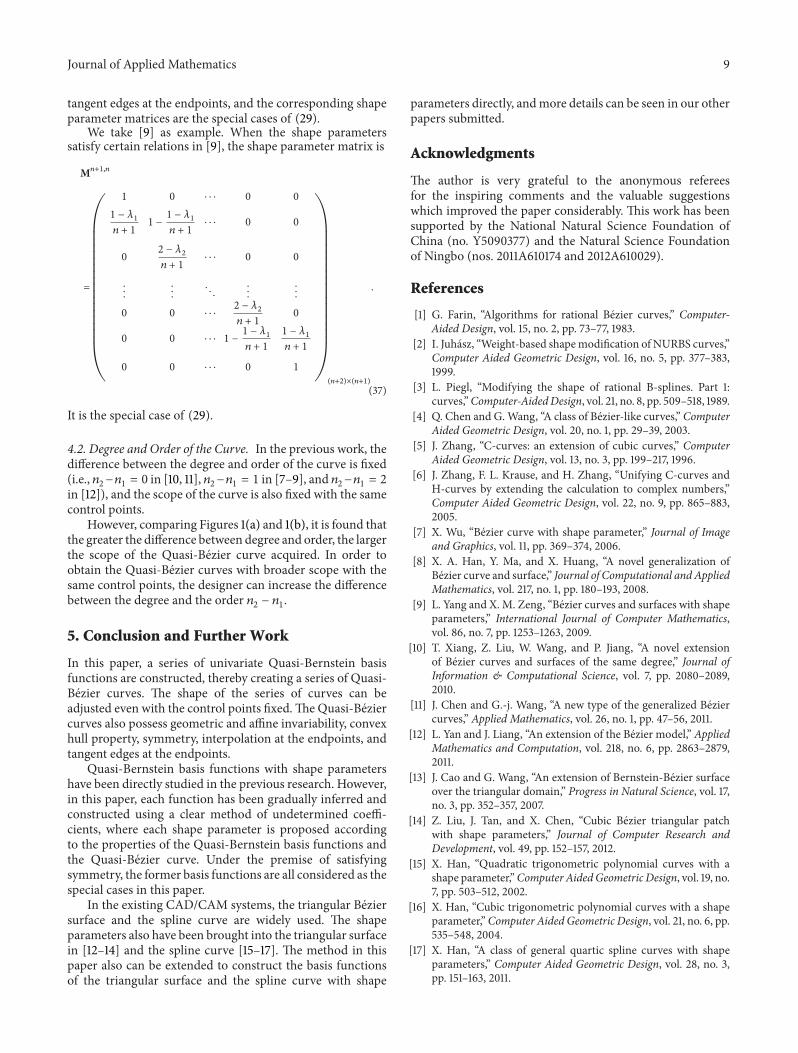