A Class of Bézier-Like Splines in Smooth Monotone

Malaysian Journal of Mathematical Sciences 3(2): 203-226 (2009)

A Class of Bézier-Like Splines in Smooth Monotone Interpolation

Ng Seou Ling, V.P. Kong and B.H. Ong School of Mathematical Sciences,

Universiti Sains Malaysia, 11800 Penang, Malaysia

E-mail: [email protected], [email protected],[email protected]

ABSTRACT

We develop a new family of curves, the quartic and quintic Bézier-like curves, and investigate the use of these curves in smooth monotonicity preserving interpolation. These polynomial curves have, besides four control points, two additional parameters for shape control. The effect of the two parameters on the curve is analysed. Conditions on these parameters for the quartic and quintic Bézier-like curves to be

monotonic are derived. Based on these conditions, a local 1C monotonicity

preserving quartic Bézier-like spline interpolation scheme is presented. A 2C

monotonicity preserving interpolation scheme is also developed where the optimal quintic Bézier-like spline interpolant is chosen through a constrained minimization of its mean curvature.

Keywords: Bézier-like spline; Monotonicity preverving; 1C monotone interpolation;

2C monotone interpolation

INTRODUCTION

In many areas of science and engineering, it is often necessary to

obtain a continuous mathematical representation of a finite set of discrete

data. It is well known that standard techniques for interpolation are often incapable of reproducing the shape of the data like monotonicity, convexity

or positivity and this may destroy the physical interpretation of the

phenomenon or the idea of the designer. This has led to considerable interest

in shape preserving interpolation problem.

The problem of monotonicity preserving interpolation has been

considered by a number of authors. Fritsch and Carlson, (1980) use the representation of Hermite cubic polynomial to derive the necessary and

sufficient conditions for a cubic to be monotone on an interval. Delbourgo

and Gregory, (1985) develop an explicit representation of a 1C piecewise

rational cubic function which can be used to solve the problem of shape

preserving interpolation. Heß and Schmidt, (1994) construct a monotonicity

Ng Seou Ling, V.P.Kong & B.H.Ong

204 Malaysian Journal of Mathematical Sciences

preserving interpolation of discrete data by quintic polynomial splines. They

show that monotonicity can be always preserved by quintic 2C -splines.

In (Jamaludin et al., 1996) the authors introduced cubic Bézier-like

curves. Based on the cubic Bézier-like basis functions, we develop in this

paper a new family of curves, the quartic and quintic Bézier-like curves. These polynomial curves are derived via a linear or quadratic convex

combination of two or three cubic Bézier-like curves which have the same

control points. With the representation of these curves in the Hermite form, their parameters are grouped in a natural way as ratios thus resulting in two

new parameters which are referred to as α and β . The effect of α and β

on the quartic and quintic curves is analyzed. They provide local control on the shape of the curve. We present the use of these Bézier-like curves in

smooth monotonicity preserving interpolation. For the piecewise quintic

curves, the second order continuity at the end points of the adjacent

segments of the curves can be attained easily by using these two parameters independently from one another. We derive the monotonicity conditions on

these parameters of the quartic Bézier-like curve. Based on these conditions,

we construct a local 1C monotonicity preserving curve interpolation scheme

using the quartic Bézier-like splines. We also derive monotonicity

conditions for the quintic Bézier-like curve and a 2C monotonicity

preserving curve interpolation scheme is developed where the optimal

quintic Bézier-like spline interpolant is chosen through a quadratic

programming.

CUBIC BÉZIER-LIKE CURVE AND ITS PROPERTIES

The representation of a cubic Bézier-like curve with parameters

,a b ∈� and control points 0 1 2 3i

V , i , , ,= , niV ∈� , n is a positive integer,

is defined in (Jamaludin et al., 1996) to be

∑=

=3

0

),;(),;(i

iiVbatFbatr , 10 ≤≤ t [1]

where the iF are cubic basis functions with

( ))2(1)1(),;( 2

0attbatF −+−= , ttabatF 2

1)1(),;( −= ,

2

2)1(),;( ttbbatF −= , ( ))2()1(1),;( 2

3bttbatF −−+= , ,a b ∈� .


Malaysian Journal of Mathematical Sciences 205

Note that the basis functions )( tFi

are controlled by two parameters

a and b . This property gives us the convenience to change the shape of the

curve without changing the control points. Some useful properties of this

basis functions are as follows:

(i) Positivity

If 3,0 ≤≤ ba , then

0),;( ≥batFi

, 10 ≤≤ t .

(ii) Partition of unity

∑=

=3

0

1),;(i

ibatF , 10 ≤≤ t .

The piecewise cubic Bézier-like curve r in [1] with control points

iV has

the following interpolatory properties at the endpoints:

0)0( Vr = ,

3)1( Vr = ,

)()0(01

VVardt

d−= , )()1(

23VVbr

dt

d−= .

For 2=n or 3 , every point on the curve in [1] lies in the convex hull

of the control polygon if 3,0 ≤≤ ba . This is a consequence of the above

properties (i) and (ii) of the basis functions.

Quartic Bézier-like Curve

Let ),;(1

batr and ),;(2

qptr be two pieces of cubic Bézier-like curves

with the same control ordinates ( : 0 3)iV i∈ ≤ ≤� but their parameters may

be different, i.e.

∑=

=3

01

),;(),;(i

iiVbatFbatr ,

∑=

=3

02

),;(),;(i

iiVqptFqptr , 10 ≤≤ t ,

where 0, >qa and ,b p∈� . Then we define ),,,;( qpbatQ which is

abbreviated as )(tQ by

1 2( ) (1 ) ( ; , ) ( ; , )Q t t r t a b t r t p q= − + , 10 ≤≤ t .



The quartic Bézier-like curve )(tQ has the interpolatory properties at the

endpoints similar to those of the cubic Bézier-like curve in [1]:

0)0( VQ = ,

3)1( VQ = ,

)()0(01

VVaQdt

d−= , )()1(

23VVqQ

dt

d−= . [2]

If 0m and 1m are the first order derivatives of Q at 0 and 1 respectively,

then by [2] and putting (1 )u t= − , we obtain

4 3 2 20 3 00 0 0 1

3 413 3

( ) 4 64 2 6 6

44

m V V p bQ t V u u t V u t m m

a q

mut V V t

+ = + + + + −

+ − +

which clearly suggests that the parameters , , ,a b p q can be grouped as

ratios /p aα = , /b qβ = . Thus )(tQ and its first order derivative can be

represented as follows:

4 3 2 20 3 00 0 0 1

3 413 3

1( ; , ) 4 6 ( )

4 2 6

44

m V VQ t V u u t V u t m m

mut V V t

α β α β+

= + + + + −

+ − +

[3]

( )( )

3 20 0 0 1

2 31 1 0 1

2( ; , ) 3 2 ( )

32

3 2 ( )3

dQ t m u u t m m m

dt

u t m m m m t

α β α β

β α

= + ∆ − + −

+ ∆ − + − +

[4]

where 03

VV −=∆ .



Quintic Bézier-like Curve

Suppose ),;(1

batr , ),;(2

qptr and 3 ( ; , )r t f g are three pieces of cubic

Bézier-like function curves with the same control ordinates

( : 0 3)iV i∈ ≤ ≤� but their parameters are different, i.e.

∑=

=3

01

),;(),;(i

iiVbatFbatr ,

∑=

=3

02

),;(),;(i

iiVqptFqptr ,

∑=

=3

03

),;(),;(i

iiVgftFgftr , 10 ≤≤ t ,

where 0, >ga and , , ,b p q f ∈� .

When these three curves are combined as a convex combination with quadratic polynomial coefficients, we obtain a quintic polynomial curve

( ; , , , , , )R t a b p q f g on ]1,0[∈t which is abbreviated as )(tR and defined

by

2 2

1 2 3( ) (1 ) ( ; , ) 2 (1 ) ( ; , ) ( ; , )R t t r t a b t t r t p q t r t f g= − + − + . [5]

The quintic Bézier-like curve )(tR has the interpolatory properties at the

endpoints similar to those of the cubic Bézier-like curve in [1]:

0)0( VR = ,

3)1( VR = ,

)()0(01

VVaRdt

d−= , )()1(

23VVgR

dt

d−= . [6]

As we have a number of parameters at our disposal, we let / 2p a= and

/ 2p q= to obtain a simpler representation for ( )R t . If in addition, 0

m and

1m are the first order derivatives of ( )R t at 0 and 1 respectively, then by

[5] and [6] with )1( tu −= , 03

VV −=∆ and grouping the parameters as

ratios /f aα = , /b gβ = , then )(tR can be represented as

.)5()73(

)37()5(),;(

5

3

4

31

32

3010

23

3010

4

00

5

0

tVtuVmtuVVmm

tuVVmmtuVmuVtR

++−+++−+

++−+++=

α

ββα

[7]



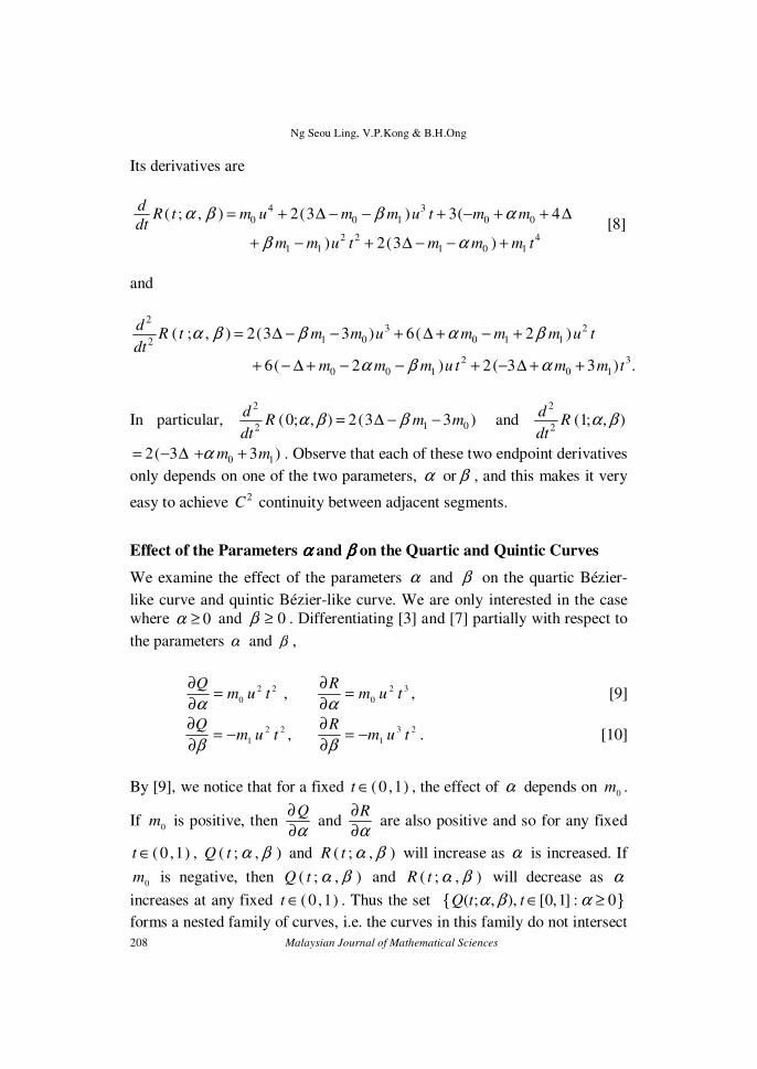
Its derivatives are

4 30 0 1 0 0

2 2 41 1 1 0 1

( ; , ) 2(3 ) 3( 4

) 2(3 )

dR t m u m m u t m m

dt

m m u t m m m t

α β β α

β α

= + ∆ − − + − + + ∆

+ − + ∆ − − + [8]

and

2

3 21 0 0 1 12

2 30 0 1 0 1

( ; , ) 2(3 3 ) 6( 2 )

6( 2 ) 2( 3 3 ) .

dR t m m u m m m u t

dt

m m m u t m m t

α β β α β

α β α

= ∆ − − + ∆ + − +

+ − ∆ + − − + − ∆ + +

In particular, 2

1 02(0; , ) 2(3 3 )

dR m m

dtα β β= ∆ − − and

2

2(1; , )

dR

dtα β

2( 3= − ∆ 0 13 )m mα+ + . Observe that each of these two endpoint derivatives

only depends on one of the two parameters, α or β , and this makes it very

easy to achieve 2C continuity between adjacent segments.

Effect of the Parameters αααα and ββββ on the Quartic and Quintic Curves

We examine the effect of the parameters α and β on the quartic Bézier-

like curve and quintic Bézier-like curve. We are only interested in the case

where 0≥α and 0≥β . Differentiating [3] and [7] partially with respect to

the parameters α and β ,

22

0tum

Q=

∂

∂

α , 32

0tum

R=

∂

∂

α, [9]

22

1 tumQ

−=∂

∂

β,

23

1 tumR

−=∂

∂

β. [10]

By [9], we notice that for a fixed )1,0(∈t , the effect of α depends on 0

m .

If 0

m is positive, then Q

α∂

∂ and

R

α∂

∂ are also positive and so for any fixed

)1,0(∈t , ),;( βαtQ and ),;( βαtR will increase as α is increased. If

0m is negative, then ),;( βαtQ and ),;( βαtR will decrease as α

increases at any fixed )1,0(∈t . Thus the set { }( ; , ), [0,1] : 0Q t tα β α∈ ≥

forms a nested family of curves, i.e. the curves in this family do not intersect



one another except at the end points 0t = and 1t = . Similarly

{ }( ; , ), [0,1] : 0R t tα β α∈ ≥ forms a nested family of curves (see Figures 1

and 4).

The effect of the parameter β depends on 1m . It is clear from [10] that, for

any fixed )1,0(∈t , if 1

m is negative, then ),;( βαtQ and ),;( βαtR

increase when β increases. If 1

m is positive, then ),;( βαtQ and

),;( βαtR will decrease as β increases at any fixed )1,0(∈t . Thus

{ }( ; , ), [0,1] : 0Q t tα β β∈ ≥ and { }( ; , ), [0,1] : 0R t tα β β∈ ≥ are also

nested families of curves (see Figures 2 and 5).

Letting µβα == and partially differentiating Q and R with respect to µ ,

we have

22

10 )( tummQ

−=∂

∂

µ, [11]

)(22

tgtuR

=∂

∂

µ,

where )()1()(10

mtmttg −−+= .

From [11], for any fixed )1,0(∈t , as µ is increased, ),;( βαtQ

increases if 010

>− mm and decreases if 0 1 0m m− < (see Figure 3). On the

other hand, the sign of R

µ∂

∂ depends directly on the sign of )(tg which is a

linear combination of 0

m and 1

m . If 00

>m and 01

>− m , then for any

fixed )1,0(∈t , )(tg is positive. Thus, for any fixed )1,0(∈t ,

),;( µµtR increases when µ is increased. If 00

<m and 01

<− m , then

0)( <tg and so for any fixed )1,0(∈t , ),;( µµtR decreases when µ

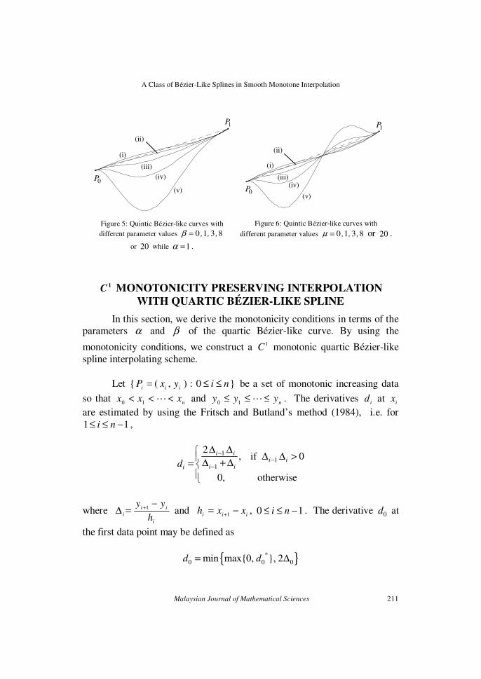
increases. If 0)(10

<− mm , )(tg will change sign at 1

0 1

mt

m m=

+. Thus,

when µ is increased, ),;( µµtR increases on the interval 1

0 1

0,m

m m

+

and decreases on 1

0 1

,1m

m m

+

or vice versa (see Figure 6).



0P

1P

(i) (ii)

(iii)

(iv)

(v)

0P

1P

(i)

(ii)

(iii) (iv)

(v)

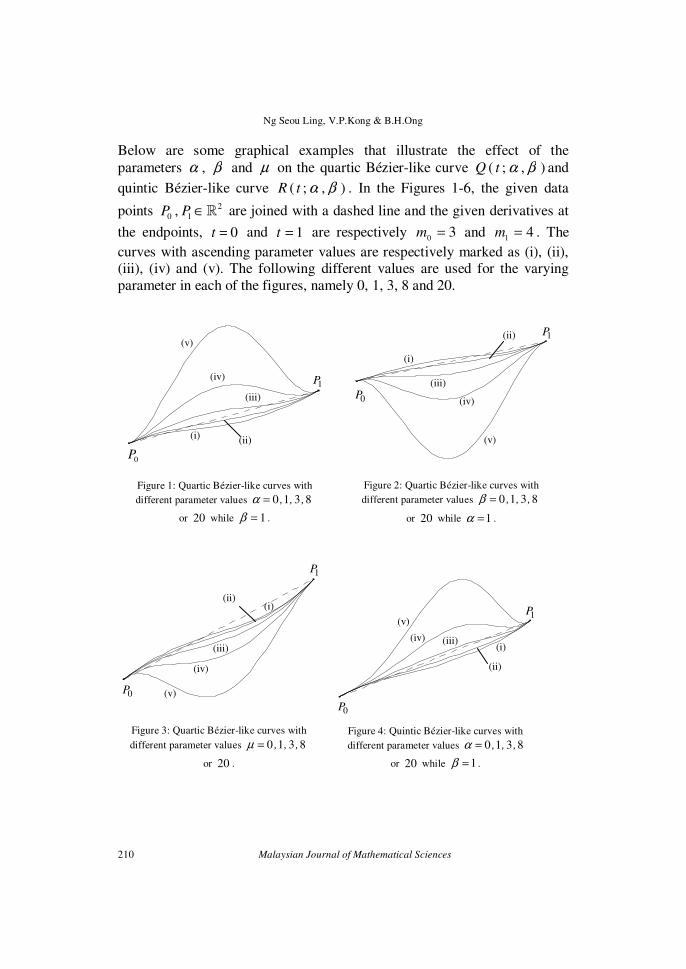
Figure 3: Quartic Bézier-like curves with

different parameter values 0 1 3 8, , ,µ =

or 20 .

Figure 4: Quintic Bézier-like curves with

different parameter values 0 1 3 8, , ,α =

or 20 while 1β = .

1P

0P

(i) (ii)

(iii)

(iv)

(v)


different parameter values 0 1 3 8, , ,α =

or 20 while 1β = .

0P

(i)

(ii)

(iii)

(iv)

(v)

1P


different parameter values 0 1 3 8, , ,β =

or 20 while 1α = .

Below are some graphical examples that illustrate the effect of the

parameters α , β and µ on the quartic Bézier-like curve ),;( βαtQ and

quintic Bézier-like curve ),;( βαtR . In the Figures 1-6, the given data

points 2

0 1,P P ∈� are joined with a dashed line and the given derivatives at

the endpoints, 0=t and 1=t are respectively 30

=m and 41

=m . The

curves with ascending parameter values are respectively marked as (i), (ii), (iii), (iv) and (v). The following different values are used for the varying

parameter in each of the figures, namely 0, 1, 3, 8 and 20.



1C MONOTONICITY PRESERVING INTERPOLATION

WITH QUARTIC BÉZIER-LIKE SPLINE

In this section, we derive the monotonicity conditions in terms of the

parameters α and β of the quartic Bézier-like curve. By using the

monotonicity conditions, we construct a 1C monotonic quartic Bézier-like

spline interpolating scheme.

Let }0:),({ niyxPiii

≤≤= be a set of monotonic increasing data

so that n

xxx <<< �10

and n

yyy ≤≤≤ �10

. The derivatives i

d at i

x

are estimated by using the Fritsch and Butland’s method (1984), i.e. for

1 1i n≤ ≤ − ,

11

1

2, if 0

0, otherwise

i ii i

i iid−

−−

∆ ∆∆ ∆ >

∆ + ∆=

where i

ii

i h

yy −=∆ +1 and

iiixxh −= +1

, 0 1i n≤ ≤ − . The derivative 0d at

the first data point may be defined as

{ }*

0 0 0min max{0, }, 2d d= ∆

0P

1P

(i)

(ii)

(iii)

(iv)

(v)


different parameter values 0 1 3 8, , ,β =

or 20 while 1α = .

1P

(ii)

(iii) (iv)

(v)

(i)

0P


different parameter values 0 1 3 8, , ,µ = or 20 .



where 0 0 2 0

* 0 11 1 2 00

1 , if 0

0 otherwise

y y

x xd

∆ ∆ − + ∆ − ∆ ≠ ∆ ∆ −=

.

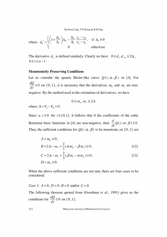
The derivative nd is defined similarly. Clearly we have 10 , 2i i id d +≤ ≤ ∆ ,

0 1i n≤ ≤ − .

Monotonicity Preserving Conditions

Let us consider the quartic Bézier-like curve ),;( βαtQ in [3]. For

0≥td

dQ on ]1,0[ , it is necessary that the derivatives 0m and 1m are non-

negative. By the method used in the estimation of derivatives, we have

∆≤≤ 2,010

mm

where 3 0 0V V∆ = − > .

Since 0, ≥tu for ]1,0[∈t , it follows that if the coefficients of the cubic

Bernstein basis functions in [4] are non-negative, then 0),;( ≥βαtQdt

d.

Thus, the sufficient conditions for ),;( βαtQ to be monotonic on ]1,0[ are

00 ≥= mA ,

0)(3

22

100≥−+−∆= mmmB βα , [12]

0)(3

22

011≥−+−∆= mmmC αβ , [13]

01 ≥= mD .

When the above sufficient conditions are not met, there are four cases to be

considered.

Case 1: 0,0,0 <>> BDA and/or 0<C

The following theorem quoted from (Goodman et al., 1991) gives us the

conditions for 0≥td

dQ on ]1,0[ .



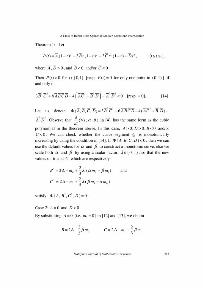
Theorem 1: Let

3223 )1(3)1(3)1()( tDttCttBtAtP +−+−+−= , 10 ≤≤ t ,

where 0, >DA , and 0<B and/or 0<C .

Then ( ) 0P t > for [0 1]t ,∈ [resp. ( ) 0P t = for only one point in (0 1), ] if

and only if

( )2 2 3 3 2 2

3 6 4 0B C ABC D AC B D A D+ − + − < [resp. = 0]. [14]

Let us denote 2 2 3 3

( , , , ) 3 6 4( )A B C D B C ABC D AC B DΦ = + − + −

2 2

A D . Observe that ( )d

Q t ; ,dt

α β in [4], has the same form as the cubic

polynomial in the theorem above. In this case, 0, 0, 0A D B> > < and/or

0C < . We can check whether the curve segment Q is monotonically

increasing by using the condition in [14]. If ( ) 0A, B, C, DΦ < , then we can

use the default values for α and β to construct a monotonic curve, else we

scale both α and β by using a scalar factor, )1,0[∈λ , so that the new

values of B and C which are respectively

)(3

22

100

* mmmB βαλ −+−∆= and

)(3

22

011

* mmmC αβλ −+−∆=

satisfy * *( , , , ) 0A B C DΦ = .

Case 2: 0=A and 0>D

By substituting 0A = (i.e. 0 0m = ) in [12] and [13], we obtain

1

22

3B mβ= ∆ − ,

11 3

22 mmC β+−∆= .



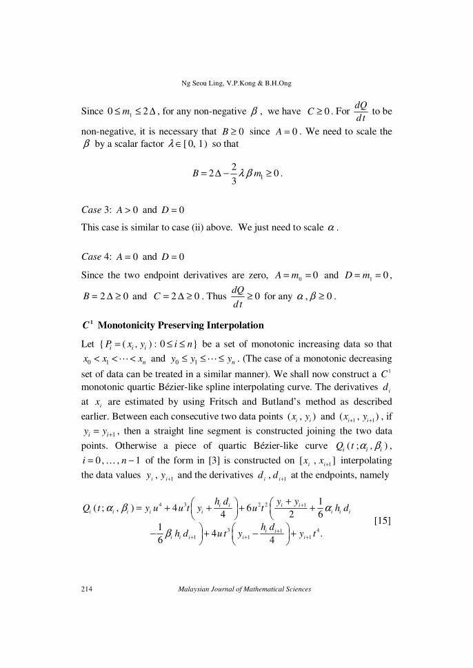
Since ∆≤≤ 201

m , for any non-negative β , we have 0≥C . For dQ

dt to be

non-negative, it is necessary that 0≥B since 0=A . We need to scale the

β by a scalar factor )1,0[∈λ so that

1

22 0

3B mλ β= ∆ − ≥ .

Case 3: 0>A and 0=D

This case is similar to case (ii) above. We just need to scale α .

Case 4: 0=A and 0=D

Since the two endpoint derivatives are zero, 00

== mA and 01

== mD ,

02 ≥∆=B and 02 ≥∆=C . Thus 0dQ

dt≥ for any 0, ≥βα .

1C Monotonicity Preserving Interpolation

Let { ( ) : 0 }i i iP x , y i n= ≤ ≤ be a set of monotonic increasing data so that

0 1 nx x x< < <� and 0 1 ny y y≤ ≤ ≤� . (The case of a monotonic decreasing

set of data can be treated in a similar manner). We shall now construct a 1C

monotonic quartic Bézier-like spline interpolating curve. The derivatives i

d

at i

x are estimated by using Fritsch and Butland’s method as described

earlier. Between each consecutive two data points ( , )i i

x y and 1 1

( , )i i

x y+ + , if

1i iy y += , then a straight line segment is constructed joining the two data

points. Otherwise a piece of quartic Bézier-like curve ( ; )i i iQ t ,α β ,

1,,0 −= ni … of the form in [3] is constructed on ],[1+ii

xx interpolating

the data values 1

, +iiyy and the derivatives

1, +iidd at the endpoints, namely

4 3 2 2 1

3 41

1 1 1

1( ; , ) 4 6

4 2 6

14 .

6 4

i i i i

i i i i i i i i

i i

i i i i i

h d y yQ t y u u t y u t h d

h dh d u t y y t

α β α

β

+

++ + +

+ = + + + +

− + − +

[15]



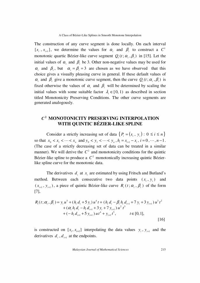
The construction of any curve segment is done locally. On each interval

],[1+ii

xx , we determine the values for i

α and i

β to construct a 1C

monotonic quartic Bézier-like curve segment ),;(iii

tQ βα in [15]. Let the

initial values of i

α and i

β be 3. Other non-negative values may be used for

iα and

iβ , but 3==

iiβα are chosen as we have observed that this

choice gives a visually pleasing curve in general. If these default values of

iα and

iβ give a monotonic curve segment, then the curve ),;(

iiitQ βα is

fixed otherwise the values of i

α and i

β will be determined by scaling the

initial values with some suitable factor )1,0[∈i

λ as described in section

titled Monotonicity Preserving Conditions. The other curve segments are

generated analogously.

2

C MONOTONICITY PRESERVING INTERPOLATION WITH QUINTIC BÉZIER-LIKE SPLINE

Consider a strictly increasing set of data ( ){ }niyxP

iii≤≤= 0:,

so that n

xxx <<< �10

andn

yyy <<< �10

,1i i i

h x x ,+= − 0 1i , , n= −� .

(The case of a strictly decreasing set of data can be treated in a similar

manner). We will derive the 2C and monotonicity conditions for the quintic

Bézier-like spline to produce a 2C monotonically increasing quintic Bézier-

like spline curve for the monotonic data.

The derivatives i

d at i

x are estimated by using Fritsch and Butland’s

method. Between each consecutive two data points ),(ii

yx and

),(11 ++ ii

yx , a piece of quintic Bézier-like curve ),;(iii

tR βα of the form

[7],

5 4 3 2

1 1

2 3

1 1

4 5

1 1 1

( ; , ) ( 5 ) ( 7 3 )

( 3 7 )

( 5 ) , [0,1],

i i i i i i i i i i i i i i

i i i i i i i

i i i i

R t y u h d y u t h d h d y y u t

h d h d y y u t

h d y ut y t t

α β β

α+ +

+ +

+ + +

= + + + − + +

+ − + +

+ − + + ∈

[16]

is constructed on 1[ , ]i ix x + interpolating the data values 1

, +iiyy and the

derivatives 1

, +iidd at the endpoints.



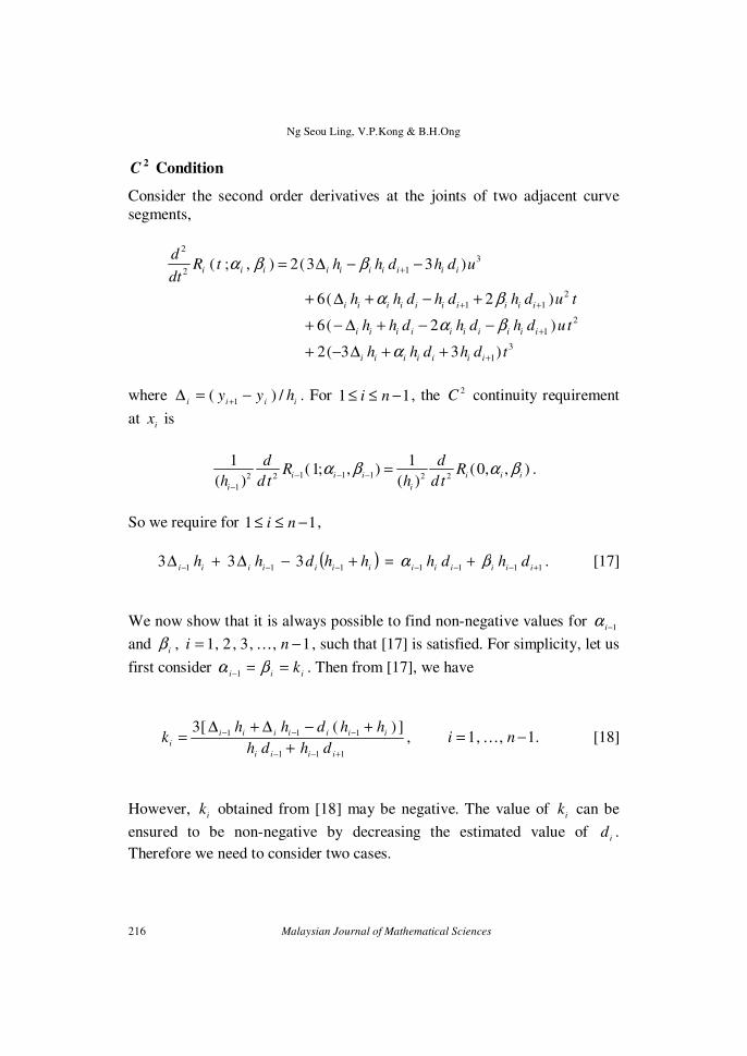
2C Condition

Consider the second order derivatives at the joints of two adjacent curve

segments,

23

12

2

1 1

2

1

3

1

( ; , ) 2(3 3 )

6( 2 )

6( 2 )

2( 3 3 )

i i i i i i i i i i

i i i i i i i i i i

i i i i i i i i i i

i i i i i i i

dR t h h d h d u

dt

h h d h d h d u t

h h d h d h d ut

h h d h d t

α β β

α β

α β

α

+

+ +

+

+

= ∆ − −

+ ∆ + − +

+ − ∆ + − −

+ − ∆ + +

where iiii

hyy /)(1

−=∆ + . For 11 −≤≤ ni , the 2C continuity requirement

at i

x is

1 1 12 2 2 2

1

1 1(1; , ) (0, , )

( ) ( )i i i i i i

i i

d dR R

h dt h dtα β α β− − −

−

= .

So we require for 11 −≤≤ ni ,

( )1111111

333 +−−−−−− +=+−∆+∆iiiiiiiiiiiii

dhdhhhdhh βα . [17]

We now show that it is always possible to find non-negative values for 1−iα

and 1,,3,2,1, −= nii

…β , such that [17] is satisfied. For simplicity, let us

first consider iii

k==− βα1

. Then from [17], we have

111

111 ])([3

+−−

−−−

+

+−∆+∆=

iiii

iiiiiii

i dhdh

hhdhhk , .1,,1 −= ni … [18]

However, i

k obtained from [18] may be negative. The value of i

k can be

ensured to be non-negative by decreasing the estimated value of i

d .

Therefore we need to consider two cases.



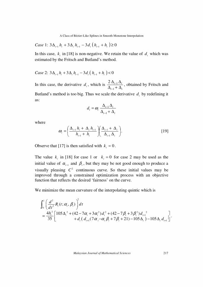
Case 1: ( ) 0333111

≥+−∆+∆ −−− iiiiiiihhdhh

In this case, i

k in [18] is non-negative. We retain the value of i

d which was

estimated by the Fritsch and Butland’s method.

Case 2: ( )1 1 13 3 3 0

i i i i i i ih h d h h− − −∆ + ∆ − + <

In this case, the derivative i

d , which is 1

1

2 i i

i i

−

−

∆ ∆

∆ + ∆, obtained by Fritsch and

Butland’s method is too big. Thus we scale the derivative i

d by redefining it

as:

1

1

i ii i

i i

d ω −

−

∆ ∆=

∆ + ∆

where

∆∆

∆+∆

+

∆+∆=

−

−

−

−−

ii

ii

ii

iiii

i hh

hh

1

1

1

11ω . [19]

Observe that [17] is then satisfied with 0=i

k .

The value i

k in [18] for case 1 or 0=i

k for case 2 may be used as the

initial value of 1−iα and

iβ , but they may be not good enough to produce a

visually pleasing 2C continuous curve. So these initial values may be

improved through a constrained optimization process with an objective

function that reflects the desired ‘fairness’ on the curve.

We minimize the mean curvature of the interpolating quintic which is

( )

221

20

2 2 2 2 2 2

1

1 1

( ; , )

4 105 (42 7 3 ) (42 7 3 ).

35 (7 7 21) 105 105

i i i

i i i i i i i i

i i i i i i i i i

dR t dt

d t

h d d

d d d

α β

α α β βα α β β

+

+ +

∆ + − + + − + = + − + + − ∆ − ∆

∫



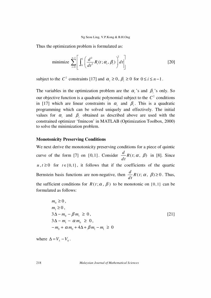
Thus the optimization problem is formulated as:

minimize

21 21

20

0

( ; , )n

i i i

i

dR t dt

dtα β

−

=

∑ ∫ [20]

subject to the 2C constraints [17] and 0,0 ≥≥ii

βα for 10 −≤≤ ni .

The variables in the optimization problem are the i

α ’s and i

β ’s only. So

our objective function is a quadratic polynomial subject to the 2C conditions

in [17] which are linear constraints in i

α and i

β . This is a quadratic

programming which can be solved uniquely and effectively. The initial

values for i

α and i

β obtained as described above are used with the

constrained optimizer ‘fmincon’ in MATLAB (Optimization Toolbox, 2000) to solve the minimization problem.

Monotonicity Preserving Conditions

We next derive the monotonicity preserving conditions for a piece of quintic

curve of the form [7] on [0,1] . Consider ( ; , )d

R tdt

α β in [8]. Since

0, ≥tu for [0,1]t ∈ , it follows that if the coefficients of the quartic

Bernstein basis functions are non-negative, then 0),;( ≥βαtRtd

d. Thus,

the sufficient conditions for ),;( βαtR to be monotonic on [ 0 , 1] can be

formulated as follows:

00

≥m ,

01

≥m ,

0310

≥−−∆ mm β , [21]

0301

≥−−∆ mm α ,

041100

≥−+∆++− mmmm βα

where 03

VV −=∆ .



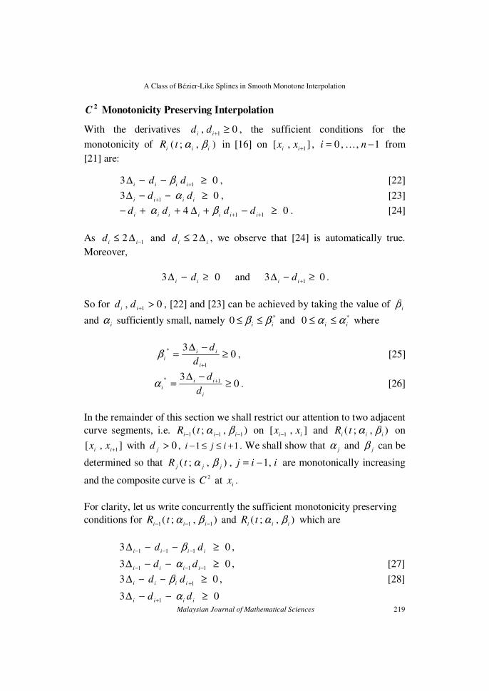
2C Monotonicity Preserving Interpolation

With the derivatives 0,1

≥+iidd , the sufficient conditions for the

monotonicity of ),;(iii

tR βα in [16] on ],[1+ii

xx , 1,,0 −= ni … from

[21] are:

031

≥−−∆ +iiiidd β , [22]

031

≥−−∆ + iiiidd α , [23]

0411

≥−+∆++− ++ iiiiiiidddd βα . [24]

As 1

2 −∆≤ii

d and ii

d ∆≤ 2 , we observe that [24] is automatically true.

Moreover,

03 ≥−∆ii

d and 031

≥−∆ +iid .

So for 0,1

>+iidd , [22] and [23] can be achieved by taking the value of

iβ

and i

α sufficiently small, namely *0ii

ββ ≤≤ and *0ii

αα ≤≤ where

03

1

*≥

−∆=

+i

ii

i d

dβ , [25]

03

1*≥

−∆= +

i

ii

i d

dα . [26]

In the remainder of this section we shall restrict our attention to two adjacent

curve segments, i.e. ),;(111 −−− iii

tR βα on ],[1 ii

xx − and ),;(iii

tR βα on

],[1+ii

xx with 0>jd , 1 1i j i− ≤ ≤ + . We shall show that jα and jβ can be

determined so that iijtR jjj ,1,),;( −=βα are monotonically increasing

and the composite curve is 2C at i

x .

For clarity, let us write concurrently the sufficient monotonicity preserving

conditions for ),;(111 −−− iii

tR βα and ),;(iii

tR βα which are

03 111 ≥−−∆ −−− iiii dd β ,

03111

≥−−∆ −−− iiiidd α , [27]

031

≥−−∆+iiii dd β , [28]

031

≥−−∆ + iiiidd α



and the 2C continuity condition at i

x from [17], i.e.

( )1111111

333 +−−−−−− +=+−∆+∆iiiiiiiiiiiii

dhdhhhdhh βα . [29]

We shall show that 1−iα and

iβ can be chosen so that conditions [27]-[29]

are satisfied. i

α and 1−iβ can be determined by using similar arguments on

the corresponding adjacent curve segments. We have shown earlier that [27]

and [28] can be achieved by taking the values of 1−iα and

iβ sufficiently

small by assuming *

110 −− ≤≤

iiαα and *0

iiββ ≤≤ where *

1−iα and *

iβ are

as defined in [26] and [25] respectively. Let us take *

11 −− =ii

αα and *

iiββ = .

However these values of 1−iα and

iβ may not satisfy the 2C continuity

condition in [29]. Here, there are two cases as in section titled 2C

Condition.

Case 1: ( ) 0333111

≥+−∆+∆ −−− iiiiiiihhdhh

In this case, the value for i

d estimated by the Fritsch and Butland’s method

is retained. In order to make equation [29] true, we have to choose the values

of 1−iα and

iβ appropriately. The values *

1−iα and *

iβ determined as in [26]

and [25] may not satisfy [29]. If it is so, we can scale the values of *

1−iα and *

iβ by a scalar, ]1,0[∈iλ . Let

*

11 −− =iii

αλα , *

iiiβλβ = . [30]

We will get the values of 1−iα and

iβ which fulfill the 2C condition [29]

and monotonicity conditions [27], [28] by substituting [30] into [29] to

obtain

( )0

3)(3

11

*

1

*

1

111 ≥+

+−∆+∆=

+−−−

−−−

iiiiii

iiiiiii

idhdh

hhdhh

βαλ .

Moreover, 1≤i

λ as shown below. From [26] and [25], we obtain

( ) ( )11

*

1

*

11113 +−−−−−− +=+−∆+∆

iiiiiiiiiiiiidhdhhhdhh βα .



So

( ) ( )11

*

1

*

111133 +−−−−−− +≤+−∆+∆

iiiiiiiiiiiiidhdhhhdhh βα .

Hence 1≤iλ . This ensures that while *

1−iα and *

iβ are being scaled by

iλ in

order to satisfy [29], the resulting values for 1−iα and

iβ still satisfy [27]

and [28].

Case 2: ( ) 0333111

<+−∆+∆ −−− iiiiiiihhdhh

In this case, the derivative id obtained by the Fritsch and Butland’s method

is too big. We shall scale down i

d accordingly by using the scalar i

ω in

[19]. With the modified derivative, [27]-[29] can be satisfied by choosing

01

=−iα and 0=i

β as our simple initial values.

The initial estimated derivatives 0

d and n

d may be 0. However, these two

cases can be similarly treated.

As a result of the discussion above, we can get the initial values for 1−iα and

iβ to satisfy the 2C and monotonicity conditions on ],[

1 iixx − and

],[1+ii

xx . We observe that 0

β on ],[10

xx and 1−n

α on ],[1 nn

xx − will not

be restricted by the 2C condition. Hence, we can choose non-negative

values for both of them which are sufficiently small to satisfy the

monotonicity conditions.

So far we have only proved that the existence of i

α and i

β , 10 −≤≤ ni for

the 2C and monotonicity conditions. But in general, the solution set

obtained as above is not necessarily good. So we will use this solution set as

the initial values to minimize the mean curvature in [20] subject to the

continuity and monotonicity linear constraints which are [17] for

1,,2,1 −= ni … , [22] and [23] for 1,,2,1,0 −= ni … and the conditions

0,0 ≥≥ii

βα to get optimal values for i

α and i

β , 10 −≤≤ ni .



GRAPHICAL EXAMPLES

We describe some graphical examples to illustrate the schemes

presented in sections titled 1C Monotonicity Preserving Interpolation with

Quartic Bézier-Like Spline and 2C Monotonicity Preserving Interpolation

with Quintic Bézier-Like Spline. The symbol ‘ • ’ shown in all of the examples represents the data point of the interpolating curve.

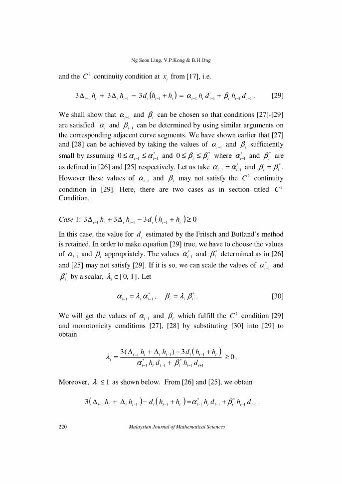
The quartic Bézier-like spline curve shown in Figure 7(a) is

generated by using the default values of 3=i

α and 3=i

β . Note that this

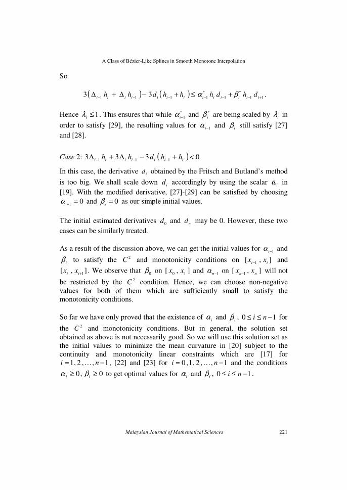
curve is not monotonic. After applying the monotonicity conditions, the

resulting curve which is shown in Figure 7(b) is now a 1C monotonic

increasing curve.

Figure 7: (b) 1C monotonicity preserving quartic

Bézier-like interpolant.

2 4 6 8 10 12 14

40

60

80

0

30

50

70

x

y

20

Figure 7: (a) 1C quartic Bézier-like interpolant.

20

40

60

80

y

30

50

70

x 0 2 4 6 8 10 12 14



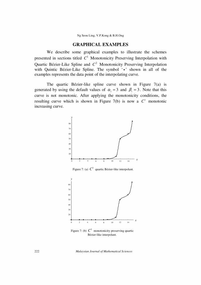
The default values 3=i

α and 3=i

β are used to construct a 1C

quartic spline curve. The curve in Figure 8(a) has a “dip” in the last curve

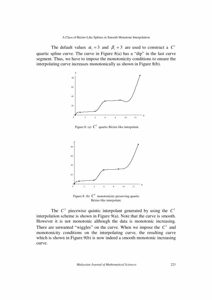
segment. Thus, we have to impose the monotonicity conditions to ensure the interpolating curve increases monotonically as shown in Figure 8(b).

The 2C piecewise quintic interpolant generated by using the 2C

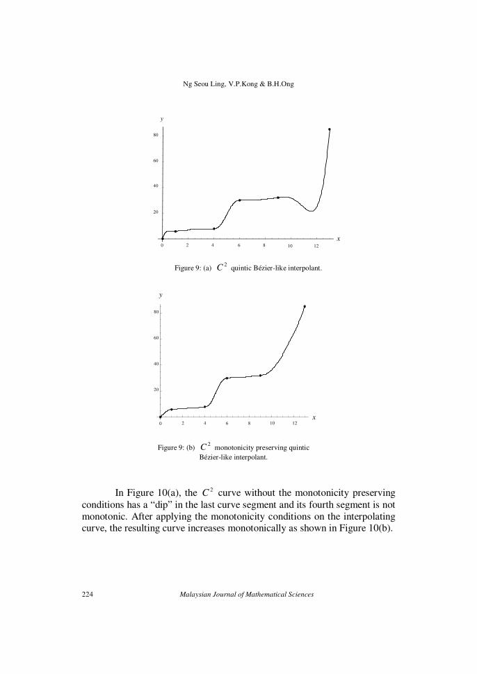
interpolation scheme is shown in Figure 9(a). Note that the curve is smooth. However it is not monotonic although the data is monotonic increasing.

There are unwanted “wiggles” on the curve. When we impose the 2C and

monotonicity conditions on the interpolating curve, the resulting curve which is shown in Figure 9(b) is now indeed a smooth monotonic increasing

curve.

2 4 6 8 10 12

y

x

80

60

40

20

0

Figure 8: (b) 1C monotonicity preserving quartic


0

20

40

60

80

2 4 6 8 10 12 x

y

Figure 8: (a) 1C quartic Bézier-like interpolant.



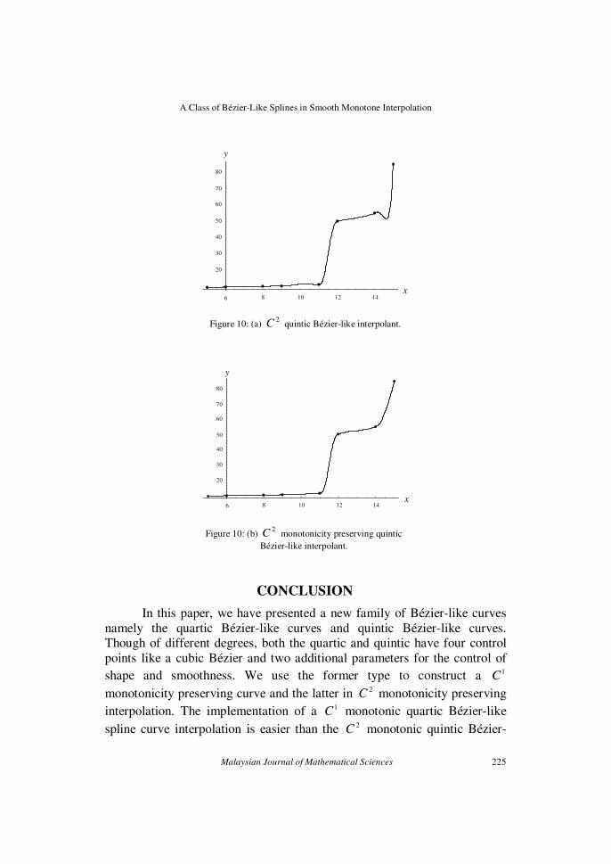
In Figure 10(a), the 2C curve without the monotonicity preserving

conditions has a “dip” in the last curve segment and its fourth segment is not

monotonic. After applying the monotonicity conditions on the interpolating curve, the resulting curve increases monotonically as shown in Figure 10(b).

Figure 9: (a) 2C quintic Bézier-like interpolant.

0

60

80

40

20

y

2 4 6 8 10 12

x

Figure 9: (b) 2C monotonicity preserving quintic


0

60

80

40

20

2 4 6 8 10 12

y

x



y

20

30

40

50

60

70

80

6 8 10 12 14 x

Figure 10: (b) 2C monotonicity preserving quintic


y

20

30

40

50

60

70

80

6 8 10 12 14 x

Figure 10: (a) 2C quintic Bézier-like interpolant.

CONCLUSION

In this paper, we have presented a new family of Bézier-like curves

namely the quartic Bézier-like curves and quintic Bézier-like curves. Though of different degrees, both the quartic and quintic have four control

points like a cubic Bézier and two additional parameters for the control of

shape and smoothness. We use the former type to construct a 1C

monotonicity preserving curve and the latter in 2C monotonicity preserving

interpolation. The implementation of a 1C monotonic quartic Bézier-like

spline curve interpolation is easier than the 2C monotonic quintic Bézier-



like spline curve interpolation since the former scheme is a local scheme.

Thus any changes to a curve segment would not affect the whole curve.

Though the latter scheme is a global scheme, it produces interpolant

which have a higher degree of smoothness. From both of the schemes that

we have constructed, we can conclude that the parameters which are introduced in the Bézier-like curves allow us flexible shape control and it is

very helpful for curve design.

ACKNOWLEDGEMENTS

The support of the FRGS Grant 203/PMATHS/671078 is

acknowledged.

REFERENCES

Delbourgo, R. and Gregory, J.A. 1985. Shape preserving piecewise rational interpolation. SIAM J. Sci. Stat. Comput. 6: 967-976.

Fritsch, F.N. and Butland, J. 1984. A method for constructing local monotone piecewise cubic interpolants. Siam J. Sci. Stat. Comput. 5:

300-304.

Fritsch, F.N. and Carlson, R.E. 1980. Monotone piecewise cubic interpolation. SIAM J. Numer. Anal. 17: 238-246.

Goodman,T.N.T., Ong, B.H. and Unsworth, K. 1991. Constrained interpolation using rational cubic splines, in NURBS for Curve and

Surface Design, ed. Gerald Farin (Philadelphia : SIAM), p.59-74.

Heß, Walter and Schmidt, Jochen W. 1994. Positive quartic, monotone

quintic 2C -spline interpolation in one and two dimensions. Journal

of Computational and Applied Mathematics, 55: 51-67.

Jamaludin, M.A., Said, H.B. and Majid, A.A. 1996. Shape control of

parametric cubic curves. In Proceedings of SPIE – The International

Society for Optical Engineering, 2644:128-133.

Optimization Toolbox User’s Guide for Use with Matlab, The Maths Works,

Inc. 2000.

Documents

A Class of Bézier-Like Splines in Smooth Monotone