213Information Technology and Control 2021/2/50

An Approximation of Bézier Curves by a Sequence of Circular Arcs

ITC 2/50Information Technology and ControlVol. 50 / No. 2 / 2021pp. 213-223DOI 10.5755/j01.itc.50.2.25178

An Approximation of Bézier Curves by a Sequence of Circular Arcs

Received 2020/01/28 Accepted after revision 2021/04/23

http://dx.doi.org/10.5755/j01.itc.50.2.25178

HOW TO CITE: Nuntawisuttiwong, T., Dejdumrong, N. (2021). An Approximation of Bézier Curves by a Sequence of Circular Arcs. Information Technology and Control, 50(2), 213-223. https://doi.org/10.5755/j01.itc.50.2.25178

Corresponding author: taweechai.wee@gmail.com

Taweechai Nuntawisuttiwong Department of Computer Engineering; King Mongkut’s University of Technology Thonburi; Bangkok, Thailand; e-mail: taweechai.wee@gmail.com

Natasha DejdumrongDepartment of Computer Engineering; King Mongkut’s University of Technology Thonburi; Bangkok, Thailand; e-mail: natasha@cpe.kmutt.ac.th

Some researches have investigated that a Bézier curve can be treated as circular arcs. This work is to propose a new scheme for approximating an arbitrary degree Bézier curve by a sequence of circular arcs. The sequence of circular arcs represents the shape of the given Bézier curve which cannot be expressed using any other al-gebraic approximation schemes. The technique used for segmentation is to simply investigate the inner angles and the tangent vectors along the corresponding circles. It is obvious that a Bézier curve can be subdivided into the form of subcurves. Hence, a given Bézier curve can be expressed by a sequence of calculated points on the curve corresponding to a parametric variable t. Although the resulting points can be used in the circular arc construction, some duplicate and irrelevant vertices should be removed. Then, the sequence of inner angles are calculated and clustered from a sequence of consecutive pixels. As a result, the output dots are now appropriate to determine the optimal circular path. Finally, a sequence of circular segments of a Bézier curve can be approx-imated with the pre-defined resolution satisfaction. Furthermore, the result of the circular arc representation is not exceeding a user-specified tolerance. Examples of approximated nth-degree Bézier curves by circular arcs are shown to illustrate efficiency of the new method.KEYWORDS: Bézier Curves, Circular arc Approximation, Analytic geometric of circle, Arbitrary degree.

1. IntroductionIn geometric modeling, there are different kinds of file formats used in design and production processes. In the design process, models are usually designed by Bézier curves and B-spline but such models cannot be directly used in the production process. Besides the

vector graphics format used in design applications, the raster graphics format is another format applied in the production process. Exchanging data between processes, shapes must be converted into arcs or lines for each supported format because arcs and lines can

Information Technology and Control 2021/2/50214

be used as media for both data form ats: vector and raster. Using only line segments, the machine will re-ceive numerous lines of code in production. Reducing lines of code, circular arcs must be used.In CAD/CAM applications Bézier curves are com-monly used because it can model complex curves with shape preservation during control point reloca-tion [4]. In the past, only quadratic and cubic Bézier curves were used to design because of some limita-tions. However, some technologies are developed to accept arbitrary degree Bézier curves for drawing models e.g. the style spline feature in SolidWorks ap-plication [19]. Thus, investigation in the arbitrary de-gree of Bézier curves is appropriate to represent the model of data exchange between design and produc-tion process with modern technologies.In manufacturing industries, Computerized Numeri-cal Control (CNC) can only support arc and line seg-ments to cut the workpieces. Typically, a nonlinear shape can only be subdivided into a sequence of line segments. The method can be called a linearization process. Linearizing with the high precision of inter-polation, it will be dramatically increased by a large number of the line segments. To improve the efficien-cy of the production of CNC machine, a quadratic Bézier curve can be approximated by a sequence of arc segments [1, 10-12, 14, 20]. The curve fitting using linear and circular-arc interpolation was first pre-sented by L. Piegl [14] in 1986. However, this method could only create a continuous path and errors always occured at the joints of subcurves. Later, this approx-imation algorithm was applied to the cases of qua-dratic Bézier curves [20]. Although convexity and C1 properties were improved by approximating methods [1, 10-12], these methods are only appropriate for the quadratic Bézier curve. Therefore, the approximation quadratic Bézier curves were used instead of the lin-earization method.As regards the cubic Bézier curves representation, subdivision method [15] was invented to improve the efficiency of approximation and to reduce the num-ber of arc segments. The subdivision strategies were applied by bisection method, developed by J. H. Yong et al. [21]. Later, the subdivision algorithm was im-proved to reduce the number of arcs by A. Riskus [16] in 2013. Besides, a Bézier curve could be described as arc splines by using Hough transform [8]. Neverthe-less, the previous circular arc approximation methods

employ recursive methods with a number of factors which cause a high computational time and the tech-niques to cubic Bézier curves were only restricted.In curve comparison or image matching, for example pattern recognition, curvature [17] is generally used as a feature for characterizing shapes. The curvature at any point of curve can be defined by the inverse of the radius of its osculating circle. Using curvature as a shape description, different primitives are identi-fied with rotation, scaling, and translation invariance. Comparing a raster image (bit-mapped image) to a vector image by extracting curvature as features [7], the vector-to-raster conversion (rasterization) can be discarded. Avoiding rasterization, vector images can keep various merits such as scalability, smoothness and continuity. Nonetheless, there are few methods used to extract curvatures suitably for simple, fast and robust implementation.Besides vector graphics formats used in applications, a sequence of points or raster images can be used as an input in industries for example trajectory robot arm. A sequence of points is approximated by arcs for sup-porting machines in production and movement of ro-botic automation. An optimal arc spline approximation was presented by G. Maier [9] in 2014. This method computes a SMAP (smooth minimum arc path) to con-struct the path of given point sequences with user-de-fined tolerance. Approximating path of robot move-ment, algorithm for planar movement was proposed in [2]. The path of robot movement was approximated by using three points to define a circle technique. Later in 2017, this technique was improved to apply in spatial movement [3]. Moreover, the velocity of the movement is increased while the size of code can be reduced.This paper focuses on circular arc approximation of nth-degree Bézier curves. The key parameter used in this study is linear interpolation of the equal-arc length portions (inscribed regular polygon) on the curve segments. Regarding the merit of polygon, cir-cular arcs can be approximated that proved in [22]. Thus, the inscribed regular polygons are treated as circular arcs on Bézier curve segments. The method to approximate Bézier curves by a sequence of arc splines with inscribed regular polygon was proposed in [13]. The cubic and quintic monotonic Bézier curves were approximated. In this research, the algo-rithm is improved for approximating arbitrary degree Bézier curves.

215Information Technology and Control 2021/2/50

Section 2 proposes a method of circular arcs approx-imation of an arbitrary degree Bézier curve by using geometric analysis of a circle. As a result, a set of cir-cular arcs for a Bézier curve approximation can be obtained. Some examples of circular arc approxima-tion of arbitrary degree Bézier curves are shown in Section 3.

2. Circular Arc Approximation for a Bézier CurveThis section presents an approximation method for a Bézier curve construction by circular arcs. Em-ploying geometric analysis, a sequence of points on a circle has been calculated with the same arc length. However, a Bézier curve can be represented in Bern-stein basis function by

0( ) ( ),

nn

i ii

t B t=

= ∑B b

where 0{ }ni ib = , are the Bézier control points, and ( )n

iB tis the Bernstein polynomial of degree n defined by

!( ) (1 t) .!( 1)!

n i n ii

nB t ti n

−= −−

Definition 1. (Sampled points on a Bézier curve). Given a Bézier curve of degree n, a sequence of control points ip , 0 i N≤ ≤ , consists of the points on the curve by substituting each parameter it into Bézier curve

( )tB . Then,

( )i ip t= B (1)

where / .it i N=For any arc lengths of ( )tB from a to b, point-based methods applied by Simpson's rule [5] is used to esti-mate the arc length of a Bézier curve as follows:

[ , ] 0 1 2

2 0 0 1 2

1( ( ) | ) (| 3 4 |64 | | | 4 3 |),

a bL B t p p p

p p p p p

≈ − + −

+ − + − +(2)

where 0 2( ), t , ,i ip t a b t= = =B and (( ) / 2).ip a b= +BLet is , 0 i N≤ ≤ , be the arc length from 0p to ip satis-fying 0 1 2 Ns s s s< < < < , where 0 0s = and Ns is the length of Bézier curve. For a large number of N , the

value of is is gradually increased. Accordingly, is can be used as the domain for sampling curves by uniform arc length. As a result, the domain of Bézier curves is changed from parameter t to space .sDefinition 2. (Equal-length sampled points). Given a sequence of Bézier sampled points, denoted by 0{ }N

i ip = , a vertex sequence on such a Bézier curve, denoted by

0 1 2{ , , , , }MV v v v v= , can be computed from sampling Bézier curve into M equal-length arc portions.By Equation (2), the arc length of each curve segment from 0v to jv is defined by

0| jv

j vL L= ,

where 0 j M≤ ≤ . Then, the equal-arc length portions must satisfy

1 1 .j j j jL L L L− +− = −

Any uniform arc vertices jv can be directly calculat-ed by assigning parametric variables, denoted by it . Then,

( )j iv t= B ,

where i is the index of arc length is at point ( )itB and it is satisfied by the condition | | 0.j iL s− →In this paper, uniform arc length vertices are used to detect circular arcs. Such a sequence of vertices will be linearly interpolated to construct an inscribed polygon in a curve. If the sides of a polygon are abun-dant, the polygon is approaching a curve. It can be implied that the error of linear interpolation depends on a number of sampled points. The more sampled points, the less error of linear interpolation.Lemma 1. A Bézier curve ( )tB has an appropriate number of uniform arc length sampled points, denoted by M , that is satisfied the given error of linear inter-polation, called tolerance (τ ) if

| ( ) | , 0 18

B tM tτ′′

= ≤ ≤ , (3)

where t is a parameter.Proof. A linear interpolating curve ( )tC in an interval [ , ]a b of ( )tB is given by

( ) ( )( ) ( ) ( ).b at a t ab a−

= + −−

B BC B (4)

Information Technology and Control 2021/2/50216

It has an error of interpolation, denoted by | ( ) ( ) | .t tε = −B C By Rolle's theorem, it is obtained:

( )( ) | ( ) |, .2

t a t b B t a t bε − − ′′= ≤ ≤ (5)

In calculus, an error ε can be maximized and sim-plified in terms of interval width, .h b a= − The max-imum ε can be considered by τ and defined as fol-lows:

2

| ( ) | .8h B tτ ′′= (6)

The relationship between width of each segment, de-noted by h , and number of sampling points, denot-ed by M , inversely varies to each other as 1/ .M h= Then, it can be concluded that

2

1 | ( ) | .8

B tM

τ ′′= (7)

Therefore,

| ( ) | .8

B tMτ′′

=

By Lemma 1, the number of sampled points can be evaluated adaptively due to the user defined toler-ance. Beside tolerance, shape and curve resolutions are also affected by interpolation error. However, shape and curve resolution depend on a set of control points that can be expressed in term of ( )tB . Hence, Lemma 1 can be applied on any shapes and resolu-tions of Bézier curves.Definition 3. (Representation of Bézier subcurves). A Bézier curve defined by a sequence of vertices,

0 1 2{ , , , , }MV v v v v= , can be subdivided into a se-quence of subcurves, denoted by 0 1 2 1{ , , , , }M −q q q q . Then, jq , where 0 1j M≤ ≤ − , is a Bézier subcurve represented by vertices, jv and 1jv + , and edge, denoted by je .By Definition 2, a vertex sequence has equal arc-length portions. Considering a set of edges, denoted by 0 1 2 1{ , , , , }ME e e e e −= , an edge je , connecting be-tween two vertices jv and 1jv + , can be acted as Bézier subcurves. Therefore, all edges are equal arc length. After choosing points on a Bézier curve, the sam-pled points, denoted by 0{ }M

i iv = , divide the curve into

M subcurves. Let subcurve iq be a part of the Bézi-er curve ( )tB with vertices iv and 1iv + . The inner angle, ka , between subcurves, 1kv − , and kv , where

1,2, , 1k M= − is the cosine of this angle formed by the vectors 1k kv v−

and 1.k kv v +

Consequently, the inner

angle ka can be calculated

1 1 1

1 1

cos .k k k kk

k k k k

v v v va

v v v v− − +

− +

⋅ =

(8)

Definition 4. (Regular polygon inscribed in Bézier subcurves). By linear interpolation, a sequence of sub-curves, denoted by 1 2{ , , , }i i i jq q q q+ + , has a sequence of edges 1 2 1{ , , , , }i i i je e e e+ + − , where 1 .i j M≤ < ≤ Such sequence of subcurves has an inscribed regular polygon if 1 2 1.i i ja a a+ + −= = =

Definition 5. (Bézier incidence matrix). Suppose that 0 1 2, , , , Mv v v v are the vertices and 0 1 2 1, , , , Me e e e −

are the edges of curve. Then, the incidence matrix with respect to this ordering of E and V is the ( 1)M M× +matrix [q ]ijQ = , where

1, when is incident with 0. otherwise

i jij

e vq = (9)

Given a sequence of vertices 0 1 2{ , , , , }Mv v v v and a sequence of edges 0 1 2 1{ , , , , }Me e e e − are correspond-ing to the Bézier curve portions, an incidence matrix of Bézier curve can be represented by

Considering the incidence matrix, the adjacent edges share a joint point joining two subcurves. Using the incidence matrix to detect circular arcs, a given se-quence of edges will be classified as a circular arc if a regular polygon can be inscribed in a given sequence -- satisfied Definition 4.Definition 6. (Interior vertices on circular path). Let

1ie − , ie , and 1ie + be a sequence of edges on a Bézier curve portion. A pair of edges, 1ie − and ie , is connected by vertex iv . Another pair of edges, ie and 1ie + is con-

217Information Technology and Control 2021/2/50

nected by vertex 1iv + . Both vertices iv and 1iv + are the interior vertices on a circular path if inner angles ia and 1ia + are equal.Definition 7. (Incidence matrix Transformation). Let

ia and 1ia + be inner angles at vertices iv and 1iv + , re-spectively. Edges ie and 1ie + will be a circular path if inner angles ia and 1ia + are equal. Then, the incidence matrix will be transformed by combining rows of edges

ie and 1ie + to circular path kc defined by

( 1)kj ij i je e += ∨c ,

where 0 .i M≤ ≤

Definition 8. (Circular path matrix). The m circular paths of an incidence matrix with 1M + vertices can be defined as the ( 1)m M× + boolean matrix { }ijC c= , in which the element in the ith row and the jth column is 1 if the ith circular path contains jth vertex; otherwise, ijc is 0.Demonstrating incidence matrix with interior verti-ces, let 0 1 2 3 4 5{ , , , , , }v v v v v v be a sequence of vertices and 0 1 2 3 4{ , , , , }e e e e e be a sequence of edges in Bézier curve portion. The incidence matrix of such a Bézier curve can be illustrated by

Assumes a sequence of inner angles to be a set 1 2 3 4{ , , , }a a a a where 1 2a a= and 3 4a a= . First, two

edges 0e and 1e are combined into a circular path 0 .c Then, incidence matrix is transformed as follows:

Considering inner angle 1a and 2a at vertices 1v and 2v respectively, the edge 2e will be merged with circular path 0c and incidence matrix is transformed as follows:

The next step of transforming the incidence matrix, inner angles 2a and 3a are considered. An incidence matrix will not be changed because inner angles 2a and 3a are not equal. The last pair of inner angles 3aand 4a are equal so the incidence matrix will be com-bined 3e and 4e to a new circular path as follows:

As a result of incidence matrix transformation in this demonstration, two circular paths are generated by merging edges with the same inner angles. Therefore, there are two circular arcs in such a Bézier curve por-tion. The first circular arc contains a sequence of ver-tices 0 1 2 3{ , , , }.v v v v Other circular arcs contain only a sequence of vertices 3 4 5{ , , }.v v v Theorem 1. A Bézier curve can be expressed by a se-quence of circular arcs, denoted by 1 2{ , , , c }mc c , where kc can be constructed by a sequence of edge kE and .m M< Then, each circular arc, the following con-ditions hold true. _

kc consists of edges kie that are incident with the same set of vertices .kjv

_ A circular arc kc is a representative for a sequence of edges kE if and only if ( 1)ki k ia a +≈ and

( 1) ( 1) ( 2) .ki k i k i k iv v v v ε+ + +− →

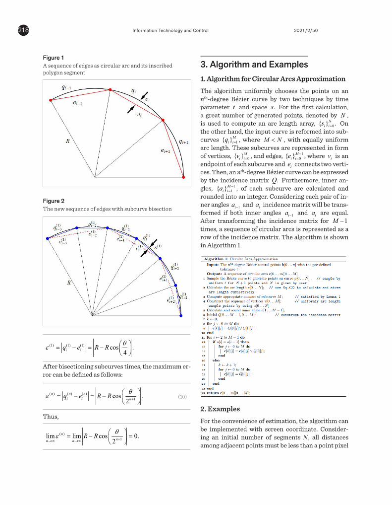
Proof. Suppose 1i−q , iq , and 1i+q are consecutive sub-curves with equal arc length. The line segment 1ie − , ie , and 1ie + are linearly interpolated in each subcurves. If all line segments have equal length and inner angle are the same, then 1 1{ , , }i i i− +q q q can be represented as cir-cular arc with radius R as demonstrated in Figure 1.For evaluating 1 1{ , , }i i i− +q q q as a circular arc, all points on these subcurves must be points on a circle with ra-dius .R Considering maximum error ε between ie and iq , it can be determined that

q cos .2i ie R R θε = − = −

The maximum error can be reduced by bisection subcurves as shown in Figure 2. By bisection of sub-curves, new subcurves, (1)

iq , are subdivided and new line segments, ie , are interpolated. Furthermore, the maximum error is reduced into

Information Technology and Control 2021/2/50218

(1) (1) (1) cos .4i iq e R R θε = − = −

After bisectioning subcurves times, the maximum er-ror can be defined as follows:

( ) ( ) ( )1cos .

2n n n

i i nq e R R θε +

= − = −

(10)

Thus,

( )1lim lim cos 0.

2n

nn nR R θε +→∞ →∞

= − =

Figure 1 A sequence of edges as circular arc and its inscribed polygon segment

3. Algorithm and Examples1. Algorithm for Circular Arcs ApproximationThe algorithm uniformly chooses the points on an nth-degree Bézier curve by two techniques by time parameter t and space .s For the first calculation, a great number of generated points, denoted by N , is used to compute an arc length array, 0{ } .N

i is = On the other hand, the input curve is reformed into sub-curves 1{ }M

i iq = , where M N< , with equally uniform arc length. These subcurves are represented in form of vertices, 0{ }M

i iv = , and edges, 10{ }M

i ie −= , where iv is an

endpoint of each subcurve and ie connects two verti-ces. Then, an nth-degree Bézier curve can be expressed by the incidence matrix .Q Furthermore, inner an-gles, 1

1{ }Mi ia −

= , of each subcurve are calculated and rounded into an integer. Considering each pair of in-ner angles 1ia − and ia incidence matrix will be trans-formed if both inner angles 1ia − and ia are equal. After transforming the incidence matrix for 1M − times, a sequence of circular arcs is represented as a row of the incidence matrix. The algorithm is shown in Algorithm 1.

Figure 2 The new sequence of edges with subcurve bisection

2. ExamplesFor the convenience of estimation, the algorithm can be implemented with screen coordinate. Consider-ing an initial number of segments N , all distances among adjacent points must be less than a point pixel

219Information Technology and Control 2021/2/50

to generate the continuous arc length parameter .is The maximum distance between two adjacent points is actually the endpoints of the curve so we must ap-proximate 1p which is next to 0p (when 0p is the first control point 0b ).Suppose that 1t is the corresponding parameter 1p , satisfied 1 1( ).p t≈ B Then, it is obtained that

1

1 .Nt

=

By Newton Raphson's method [18], the parameter 1t can be approximated by

0 1 01 0

0 1 0

( ( ) ) ( ),

[( ( ) ) ( )]t p t

t tt p t

′−= −

′ ′−B BB B

(11)

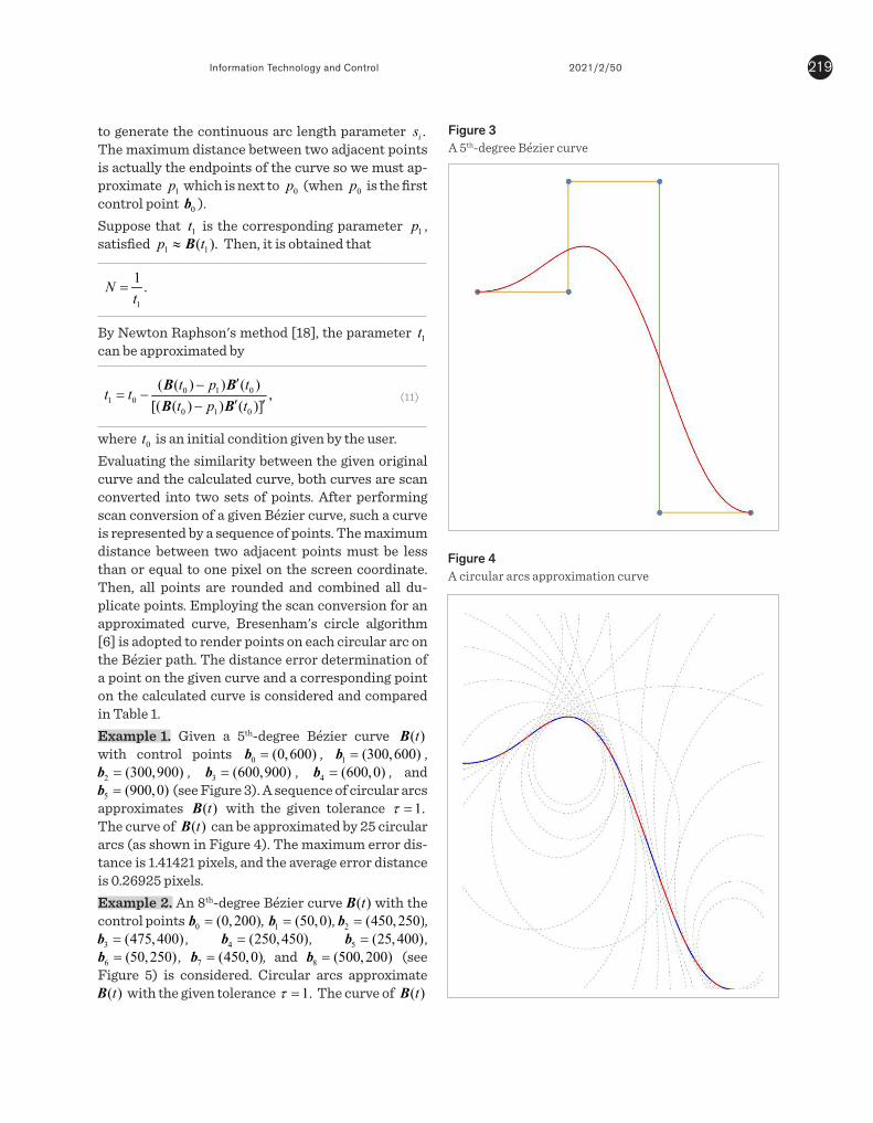
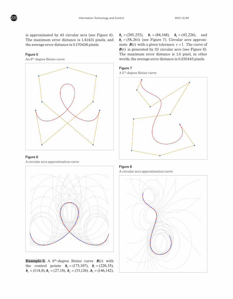
where 0t is an initial condition given by the user.Evaluating the similarity between the given original curve and the calculated curve, both curves are scan converted into two sets of points. After performing scan conversion of a given Bézier curve, such a curve is represented by a sequence of points. The maximum distance between two adjacent points must be less than or equal to one pixel on the screen coordinate. Then, all points are rounded and combined all du-plicate points. Employing the scan conversion for an approximated curve, Bresenham's circle algorithm [6] is adopted to render points on each circular arc on the Bézier path. The distance error determination of a point on the given curve and a corresponding point on the calculated curve is considered and compared in Table 1.Example  1. Given a 5th-degree Bézier curve ( )tB with control points 0 (0,600)=b , 1 (300,600)=b ,

2 (300,900)=b , 3 (600,900)=b , 4 (600,0)=b , and 5 (900,0)=b (see Figure 3). A sequence of circular arcs

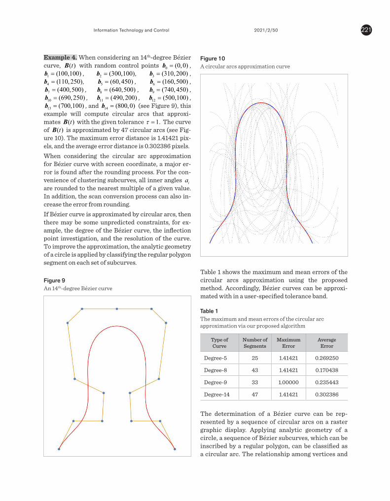
approximates ( )tB with the given tolerance 1.τ = The curve of ( )tB can be approximated by 25 circular arcs (as shown in Figure 4). The maximum error dis-tance is 1.41421 pixels, and the average error distance is 0.26925 pixels.Example  2. An 8th-degree Bézier curve ( )tB with the control points 0 (0, 200)=b , 1 (50,0)=b , 2 (450,250)=b ,

3 (475,400)=b , 4 (250,450)=b , 5 (25,400)=b , 6 (50,250)=b , 7 (450,0)=b , and 8 (500,200)=b (see

Figure 5) is considered. Circular arcs approximate ( )tB with the given tolerance 1.τ = The curve of ( )tB

Figure 3 A 5th-degree Bézier curve

Figure 4 A circular arcs approximation curve

Information Technology and Control 2021/2/50220

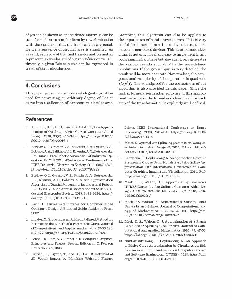
is approximated by 43 circular arcs (see Figure 6). The maximum error distance is 1.41421 pixels, and the average error distance is 0.170438 pixels.

Figure 5 An 8th-degree Bézier curve

Figure 6 A circular arcs approximation curve

6 (205,252)=b , 7 (84,168)=b , 8 (43,226)=b , and 9 (58,261)=b (see Figure 7). Circular arcs approxi-

mate ( )tB with a given tolerance 1.τ = The curve of ( )tB is generated by 33 circular arcs (see Figure 8).

The maximum error distance is 1.0 pixel, in other words, the average error distance is 0.235443 pixels.

Figure 7 A 5th-degree Bézier curve

Figure 8 A circular arcs approximation curve

Example  3. A 9th-degree Bézier curve ( )tB with the control points 0 (175,107)=b , 1 (220,35)=b ,

2 (114,0)=b , 3 (27,18)=b , 4 (33,126)=b , 5 (146,142)=b ,

221Information Technology and Control 2021/2/50

Example 4. When considering an 14th-degree Bézier curve, ( )tB with random control points 0 (0,0)=b ,

1 (100,100)=b , 2 (300,100)=b , 3 (310,200)=b , 4 (110,250)=b , 5 (60,450)=b , 6 (160,500)=b , 7 (400,500)=b , 8 (640,500)=b , 9 (740,450)=b , 10 (690,250)=b , 11 (490,200)=b , 12 (500,100)=b , 13 (700,100)=b , and 14 (800,0)=b (see Figure 9), this

example will compute circular arcs that approxi-mates ( )tB with the given tolerance 1.τ = The curve of ( )tB is approximated by 47 circular arcs (see Fig-ure 10). The maximum error distance is 1.41421 pix-els, and the average error distance is 0.302386 pixels.When considering the circular arc approximation for Bézier curve with screen coordinate, a major er-ror is found after the rounding process. For the con-venience of clustering subcurves, all inner angles ia are rounded to the nearest multiple of a given value. In addition, the scan conversion process can also in-crease the error from rounding.If Bézier curve is approximated by circular arcs, then there may be some unpredicted constraints, for ex-ample, the degree of the Bézier curve, the inflection point investigation, and the resolution of the curve. To improve the approximation, the analytic geometry of a circle is applied by classifying the regular polygon segment on each set of subcurves.

Figure 9 An 14th-degree Bézier curve

Table 1 shows the maximum and mean errors of the circular arcs approximation using the proposed method. Accordingly, Bézier curves can be approxi-mated with in a user-specified tolerance band.

Figure 10 A circular arcs approximation curve

Table 1The maximum and mean errors of the circular arc approximation via our proposed algorithm

Type of Curve

Number of Segments

MaximumError

AverageError

Degree-5 25 1.41421 0.269250

Degree-8 43 1.41421 0.170438

Degree-9 33 1.00000 0.235443

Degree-14 47 1.41421 0.302386

The determination of a Bézier curve can be rep-resented by a sequence of circular arcs on a raster graphic display. Applying analytic geometry of a circle, a sequence of Bézier subcurves, which can be inscribed by a regular polygon, can be classified as a circular arc. The relationship among vertices and

Information Technology and Control 2021/2/50222

edges can be shown as an incidence matrix. It can be transformed into a simpler form by row elimination with the condition that the inner angles are equal. Hence, a sequence of circular arcs is simplified. As a result, each row of the final transformation matrix represents a circular arc of a given Bézier curve. Ul-timately, a given Bézier curve can be expressed in terms of these circular arcs.

4. ConclusionsThis paper presents a simple and elegant algorithm used for converting an arbitrary degree of Bézier curve into a collection of consecutive circular arcs.

Moreover, this algorithm can also be applied to the input cases of hand-drawn curves. This is very useful for contemporary input devices, e.g., touch-screen or pen-based devices. This approximate algo-rithm is not only novel and easy to implement in any programming language but also adaptively generates the various results according to the user-defined resolutions. If the given input is very detailed, the result will be more accurate. Nonetheless, the com-putational complexity of the operation is quadratic

2( ( )).O n The soundproof for the correctness of our algorithm is also provided in this paper. Since the matrix formulation is adopted to use in this approx-imation process, the formal and clear proof for each step of the transformation is explicitly well-defined.

References 1. Ahn, Y. J., Kim, H. O., Lee, K. Y. G1 Arc Spline Approx-

imation of Quadratic Bézier Curves. Computer-Aided Design, 1998, 30(6), 615-620. https://doi.org/10.1016/S0010-4485(98)00016-5

2. Borisov, O. I., Gromov, V. S., Kolyubin, S. A., Pyrkin, A. A., Bobtsov, A. A., Salikhov, V. I., Klyunin, A. O., Petranevsky, I. V. Human-Free Robotic Automation of Industrial Op-eration. IECON 2016, 42nd Annual Conference of the IEEE Industrial Electronics Society, 2016, 6867-6872. https://doi.org/10.1109/IECON.2016.7793922

3. Borisov, O. I., Gromov, V. S., Pyrkin, A. A., Petranevsky, I. V., Klyunin, A. O., Bobstov, A. A. Arc Approximation Algorithm of Spatial Movements for Industrial Robots. IECON 2017 - 43nd Annual Conference of the IEEE In-dustrial Electronics Society, 2017, 3429-3434. https://doi.org/10.1109/IECON.2017.8216581

4. Farin, G. Curves and Surfaces for Computer Aided Geometric Design: A Practical Guide. Academic Press, 2002.

5. Floater, M. S., Rasmussen, A. F. Point-Based Method for Estimating the Length of a Parametric Curve. Journal of Computational and Applied mathematics, 2006, 196, 512-522. https://doi.org/10.1016/j.cam.2005.10.001

6. Foley, J. D., Dam, A. V., Feiner, S. K. Computer Graphics, Principles and Pratice, Second Edition in C. Pearson Education Inc., 1996.

7. Hayashi, T., Kiyono, T., Abe, K., Onai, R. Retrieval of 2D Vector Iamges by Matching Weighted Feature

Points. IEEE International Conference on Image Processing, 2008, 961-964. https://doi.org/10.1109/ICIP.2008.4711916

8. Maier, G. Optimal Arc Spline Approximation. Comput-er Aided Geometric Design 31, 2014, 211-226. https://doi.org/10.1016/j.cagd.2014.02.011

9. Kaewsaiha, P., Dejdumrong, N. An Approach to Describe Parametric Curves Using Hough-Based Arc Spline Ap-proximation. 11th International Conference on Com-puter Graphics, Imaging and Visualization, 2014, 5-10. https://doi.org/10.1109/CGiV.2014.14

10. Meek, D. S., Walton, D. J. Approximating Quadratics NURBS Curves by Arc Splines. Computer-Aided De-sign, 1993, 25, 371-376. https://doi.org/10.1016/0010-4485(93)90032-J

11. Meek, D. S., Walton, D. J. Approximating Smooth Planar Curves by Arc Splines. Journal of Computational and Applied Mathematics, 1995, 59, 221-231. https://doi.org/10.1016/0377-0427(94)00029-Z

12. Meek, D. S., Walton, D. J. Approximation of a Planar Cubic Bézier Spiral by Circular Arcs. Journal of Com-putational and Applied Mathematics, 1996, 75, 47-56. https://doi.org/10.1016/S0377-0427(96)00056-8

13. Nuntawisuttiwong, T., Dejdumrong, N. An Approach to Bézier Curve Approximation by Circular Arcs. 15th International Joint Conference on Computer Science and Software Engineering (JCSSE), 2018. https://doi.org/10.1109/JCSSE.2018.8457180

223Information Technology and Control 2021/2/50

14. Piegl, L. Curve Fitting Algorithm for Rough Cutting. Computer-Aided Design, 1986, 18(2), 79-82. https://doi.org/10.1016/0010-4485(86)90154-5

15. Rueda, S., Udupa, J. K., Bai, L. Local Curvature Scale: A New Concept of Shape Description. Medical Imag-ing 2008: Image Processing, 2008, 6914. https://doi.org/10.1117/12.770444

16. Riskus, A. Approximation of a Cubic Bézier Curve by Circular Arc and Vice Versa. Informaiton Technology and Control, 2006, 35(4), 371-378.

17. Riskus, A., Liutkus, G. An Improved Algorithm for the Approximation of a Cubic Bézier and Its Application for Approximating Quadratic Bézier Curve. Informaiton Technology and Control, 2013, 42(4), 303-308. https://doi.org/10.5755/j01.itc.42.4.1707

18. Schneider, P. J. Phoenix: An Interactive Curve De-sign System Based on the Automatic Fitting of Hand-

Sketched Curves. Master's thesis, University of Wash-ington, 1998.

19. Verma G., Weber M. Solidworks 2020 Black Book (Col-ored), CADCAMCAE WORKS, 2019.

20. Walton, D. J., Meek, D. S. Approximation of Quadratic Bézier Curve by Arc Splines. Journal of Computation-al and Applied Mathematics, 1994, 54, 107-120. https://doi.org/10.1016/0377-0427(94)90398-0

21. Yonga, J. H., Hua, S. M., Sun, J. G. Bisection Algorithms for Approximating Quadratic Bézier Curves by G1 Arc Splines. Computer-Aided Design, 2000, 32, 253-260. https://doi.org/10.1016/S0010-4485(99)00100-1

22. Zygmunt, M. Circular Arc Approximation Using Poly-gons. Journal of Computational and Applied Math-ematics 322, 2017, 81-85. https://doi.org/10.1016/j.cam.2017.03.030

This article is an Open Access article distributed under the terms and conditions of the Creative Commons Attribution 4.0 (CC BY 4.0) License (http://creativecommons.org/licenses/by/4.0/).