RESEARCH Open Access Effect of network parameters on

RESEARCH Open Access

Effect of network parameters on neighborwireless link breaks in GPSR protocol andenhancement using mobility prediction modelRaed A Alsaqour1*, Maha S Abdelhaq1 and Ola A Alsukour2

Abstract

The greedy perimeter stateless routing (GPSR) protocol is a well-known position-based routing protocol. Datapacket routing in position-based routing protocols uses the neighbors’ geographical position information, which isstored in the sender’s neighbors list, and the destination’s position information stored in the routing data packetheader field to route the packet from source to destination. In the GPSR protocol, the sender routes the packets toa neighboring node, whose geographical position is the closest to the destination of all the sender’s neighbors.However, the selected neighbor is closer to the edge of the maximum of the sender’s transmission range and thushas a higher likelihood of leaving the transmission range of the sender. Thus, the wireless link between the sendernode and its routing neighboring node may break down, which degrades the performance of the routingprotocol. In this study, we identify and study the effects of network parameters (beacon packet interval-time, nodespeed, network density, transmission range, and network area size) on wireless link breakage, identified as theneighbor wireless link break (NWLB) problem, in the GPSR protocol. To overcome the NWLB problem, we proposea neighbor wireless link break prediction (NWLBP) model. The NWLBP model predicts the accurate position of arouting neighboring node in the sender’s neighbors list before routing the data packet to that neighbor. Thesimulation results show the ability of the NWLBP model to overcome the observed problem and to improve theoverall performance of the GPSR protocol.

Keywords: GPSR, position-based routing protocol, neighbor wireless link break, mobility prediction

1. IntroductionIn Mobile Ad hoc Network (MANET) position-basedrouting protocols such as DREAM, LAR, and GPSR [1],the data packet routing decision is based purely on thelocal geographical position information knowledge ofthe node’s neighbors. Each node forming the networkmust be able to determine its own geographical positioninformation (x, y coordinates) using a Global PositionSystem (GPS) device [2]. In addition, each node needsto maintain accurate geographical position informationon its immediate neighbors to make effective routingdecisions. For this purpose, each node within a deter-mined time interval, periodically broadcasts a short bea-con packet to announce its presence and geographical

position information to those of its neighbors that arewithin its transmission range. However, the geographicalposition information of all known neighboring nodes isrecorded by the receiving nodes in their lists of neigh-bors. Later, the node uses the neighbors’ position infor-mation from its list of neighbors for routing a datapacket to its destination. If a node fails to receive a bea-con packet from the corresponding neighboring nodeover a certain time interval, the node will remove thatneighbor from its list of neighbors.A highly dynamic topology is a distinguishing feature

and one of the challenges of MANET. Wireless linksa

between nodes are created and broken as the nodesmove within one another’s transmission ranges. Further-more, as the nodes move, the topology of the networkchanges rapidly and unpredictably. Nodes may join orleave the network abruptly or gradually. As a result ofnode mobility, the established wireless links between the

* Correspondence: [email protected] of Computer Science, Faculty of Information Science andTechnology, University Kebangsaan Malaysia, 43600 Bangi, Selangor, MalaysiaFull list of author information is available at the end of the article

Alsaqour et al. EURASIP Journal on Wireless Communications and Networking 2012, 2012:171http://jwcn.eurasipjournals.com/content/2012/1/171

© 2012 Alsaqour et al; licensee Springer. This is an Open Access article distributed under the terms of the Creative CommonsAttribution License (http://creativecommons.org/licenses/by/2.0), which permits unrestricted use, distribution, and reproduction inany medium, provided the original work is properly cited.

brought to you by COREView metadata, citation and similar papers at core.ac.uk

provided by Springer - Publisher Connector

https://core.ac.uk/display/81845627?utm_source=pdf&utm_medium=banner&utm_campaign=pdf-decoration-v1

mailto:[email protected]

http://creativecommons.org/licenses/by/2.0

nodes may break and require re-establishing. Moreover,the position information in the nodes’ lists of neighborsis often inaccurate and does not reflect the actual posi-tions of the neighboring nodes, thus requiring theretransmission and rerouting of the data packetsbetween nodes. However, the correctness and accuracyof position information in the node’s list of neighbors iscrucial and fundamental in determining the performanceof position-based routing protocols [3]. Existing posi-tion-based routing protocols assume implicitly or expli-citly the availability of accurate position information inthe nodes’ lists of neighbors, while in reality only animprecise estimate of this position information is avail-able for the nodes.Inaccurate information on the position of nodes may

result in a node being wrongly listed as within its neigh-bors’ transmission range. This problem has serious con-sequences for network performance because nodes inposition-based routing protocols depend on each otherfor routing the data packets to their destination, andbecause they move quickly at a uniform or non-uniformspeed, wireless links between them are unstable andeasily broken. We call this phenomenon the neighborwireless link break (NWLB) problem.In this study, we identify the problem of NWLB

between the sender node and its routing neighboringnodes in GPSR protocol. In addition, we identify andanalyze the network parameters that affect this problem,which are the beacon packet interval-time (BPIT), nodespeed (NS), network density, transmission range, andnetwork area size. Finally, to solve this problem, we pro-pose a mobility prediction model that can provide accu-rate position information on its neighbors to the sendernode at the time of the routing process. This helps thesender node to route the data packet to a suitableneighbor on its list.The rest of the article is organized as follows. In Sec-

tion 2, we provide the background, review related work,and outline the limitations of current mobility

prediction models. In Section 3, the NWLB problem isidentified. In Section 4, the effect of network parametersis analyzed and discussed. In Section 5, the mobility pre-diction model is introduced. Section 6 presents thesimulation results and evaluation, and Section 7 presentsthe conclusions and possible direction of future work inthis area.

2. Background and related work2.1. The GPSR protocolThe GPSR protocol [4] is an efficient and scalable rout-ing protocol in MANETs. In the GPSR protocol, nodesroute the data packet using the locations of its one-hopneighbors. When a node sends a data packet, it trans-mits it to the neighbor within its transmission rangethat has the shortest Euclidean distance to the destina-tion node.The GPSR protocol uses two forwarding strategies to

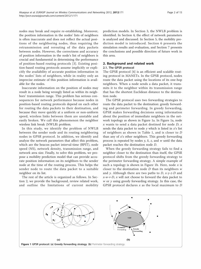
route the data packet to the destination: greedy forward-ing and perimeter forwarding. In greedy forwarding,GPSR makes forwarding decisions using informationabout the position of immediate neighbors in the net-work topology as shown in Figure 1a. In Figure 1a, nodex wants to send a data packet destined for node D; xsends the data packet to node y which is listed in x’s listof neighbors as shown in Table 1, and is closer to Dthan any of x’s other neighbors. This greedy forwardingprocess is repeated by nodes y, k, z, and w until the datapacket reaches the destination node D.When the greedy forwarding strategy fails to find a

neighbor closer to the destination than itself, the GPSRprotocol shifts from the greedy forwarding strategy tothe perimeter forwarding strategy. A simple example ofsuch a topology is shown in Figure 1b. Here, node x iscloser to the destination node D than its neighbors wand y. Although there are two paths to D, x-y-z-D andx-w-v-D, x will not choose to forward the data packet tow or y using greedy forwarding strategy. In this case, theGPSR protocol declares x as the local maximum to D

Figure 1 GPSR protocol: (a) Greedy forwarding strategy. (b) Perimeter forwarding strategy.


Page 2 of 15

and the shaded region without nodes as a void region.To route the data packet around the void region, theperimeter forwarding strategy constructs a planarizedgraphb for the neighbors of node x and routes the datapacket around the void region using the right-hand rule.The right-hand rule states that when arriving at node xfrom y, the next traversed edge is the one sequentiallycounterclockwise about x from edge (x, y). By applyingthe right-hand rule in Figure 1b, node x forwards thedata packet to hop w.

2.2. Related workSeveral mobility prediction approaches and techniqueshave been proposed in the literature for MANET rout-ing protocols. The details of these approaches and tech-niques can be found in [5]. We survey here the mobilityprediction research efforts in predicting the connectivityof the neighboring nodes based on the position informa-tion of the nodes.Jia et al. [6] proposed a two-hop Hello protocol (T-

Hello) aiming to improve the accuracy of the list ofneighbors. By exchanging beacon packet messageswithin the two-hop scope, neighbor location informationcan be obtained, even if a neighbor has moved out ofthe sender’s communication range, so the correspondingentry in the neighbor tables of the nodes can beremoved explicitly rather than waiting for time out.However, using two-hop hello beacon packet messageswill increase the chances of beacon packets collidingwith data packets and thus increase the number ofretransmissions, resulting in increasing end-to-end delayand wastage of battery power [7]. Creixell and Sezaki [8]proposed a geographical routing protocol which makesrouting decisions based on the current and future posi-tions of the node. To estimate the future position of thenode, the authors used a prediction method based onreal trajectory data. The disadvantage of this approach isin the implementation cost. The authors used singlelow-range laser scanners to track the pedestrian trajec-tory movements of the nodes, which necessitated a highstorage space for the neighbors table because they usedit to save the historical movements of the neighboringnodes.Kai-Ten et al. [9] proposed the velocity-aided routing

(VAR) protocol, which determines its data packet

routing based on the relative velocity between theintended routing node and the destination node. TheVAR protocol incorporates the predictive moving beha-viors of mobile nodes in the protocol design. Xu et al.[10] proposed a mobility prediction mechanism toacquire neighborhood information at a future actualtransmission time. In this prediction mechanism, thesender node will only send a request to collect informa-tion on neighbors before the transmission process,thereby conserving the energy consumption of periodicalbeacon packets; once the neighboring nodes receive theposition request command, they will send two beaconpackets at a specific interval. Based on received positionswithin beacon packets, the sender will predict the posi-tions of its neighboring nodes at a future transmissiontime. Son et al. [11] proposed two mobility predictionschemes; neighbor position prediction and destinationposition prediction, to overcome lost link and loop pro-blems in position-based routing protocols. The authorsbuilt their prediction schemes based on the positioninformation of two beacon packets and the beacon timeof neighboring nodes stored in the lists of neighboringnodes. Shah and Nahrstedt [12] proposed a position-delay prediction scheme which assists Quality of Servicerouting protocols to estimate a future instant positionbased on information on previous positions. Su et al.[13] proposed a simple prediction method. They calcu-lated the route expiry time Dt during which two nodes iand j will stay connected to each other. The same pre-diction time approach is used by Sandulescu andNadjm-Tehrani [14]. The authors exploited the contextof mobile nodes information, such as the speed andradio range, to estimate the contact window time tcwbetween two meeting neighbors.Cadger et al. [15] explored and analyzed the location-

prediction schemes proposed in [11,12]. Both wereimplemented on top of the GPSR protocol. The resultsindicated that the addition of location prediction toGPSR overwhelmingly improved its reliabilityperformance.

2.3. Limitations of current mobility prediction modelsIn addition to the previously observed and discussedlimitations of mobility prediction models, most of thecurrent research in mobility predictions is based on pie-cewise linear node motion between successive beaconpacket updates. In addition, it assumes that the mobilenodes move at constant speed without consideringdirection information in the beacon packet updates orprediction techniques used. Furthermore, currentresearch built mobility prediction models based on twoor more beacon packet updates.This study argues that two or more beacon packet

updates are not available to the sender on its neighbors

Table 1 Node x neighbors list

Node-id Neighbor (x, y coordinates)

A A (x1, y1)

B B (x2, y2)

C C (x3, y3)

F F (x4, y4)

y y (x5, y5)


Page 3 of 15

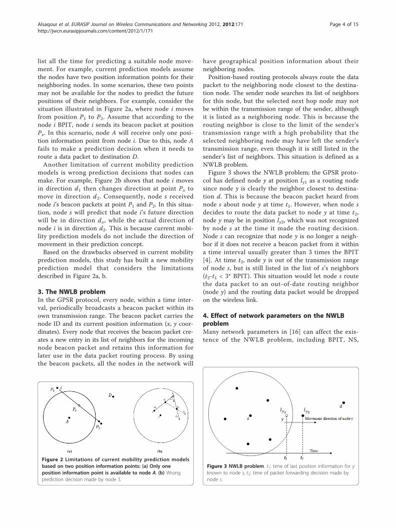
list all the time for predicting a suitable node move-ment. For example, current prediction models assumethe nodes have two position information points for theirneighboring nodes. In some scenarios, these two pointsmay not be available for the nodes to predict the futurepositions of their neighbors. For example, consider thesituation illustrated in Figure 2a, where node i movesfrom position P1 to P2. Assume that according to thenode i BPIT, node i sends its beacon packet at positionPx. In this scenario, node A will receive only one posi-tion information point from node i. Due to this, node Afails to make a prediction decision when it needs toroute a data packet to destination D.Another limitation of current mobility prediction

models is wrong prediction decisions that nodes canmake. For example, Figure 2b shows that node i movesin direction d1 then changes direction at point Px tomove in direction d2. Consequently, node s receivednode i’s beacon packets at point P1 and P2. In this situa-tion, node s will predict that node i’s future directionwill be in direction dx, while the actual direction ofnode i is in direction d2. This is because current mobi-lity prediction models do not include the direction ofmovement in their prediction concept.Based on the drawbacks observed in current mobility

prediction models, this study has built a new mobilityprediction model that considers the limitationsdescribed in Figure 2a, b.

3. The NWLB problemIn the GPSR protocol, every node, within a time inter-val, periodically broadcasts a beacon packet within itsown transmission range. The beacon packet carries thenode ID and its current position information (x, y coor-dinates). Every node that receives the beacon packet cre-ates a new entry in its list of neighbors for the incomingnode beacon packet and retains this information forlater use in the data packet routing process. By usingthe beacon packets, all the nodes in the network will

have geographical position information about theirneighboring nodes.Position-based routing protocols always route the data

packet to the neighboring node closest to the destina-tion node. The sender node searches its list of neighborsfor this node, but the selected next hop node may notbe within the transmission range of the sender, althoughit is listed as a neighboring node. This is because therouting neighbor is close to the limit of the sender’stransmission range with a high probability that theselected neighboring node may have left the sender’stransmission range, even though it is still listed in thesender’s list of neighbors. This situation is defined as aNWLB problem.Figure 3 shows the NWLB problem; the GPSR proto-

col has defined node y at position ly1 as a routing nodesince node y is clearly the neighbor closest to destina-tion d. This is because the beacon packet heard fromnode s about node y at time t1. However, when node sdecides to route the data packet to node y at time t2,node y may be in position ly2, which was not recognizedby node s at the time it made the routing decision.Node s can recognize that node y is no longer a neigh-bor if it does not receive a beacon packet from it withina time interval usually greater than 3 times the BPIT[4]. At time t2, node y is out of the transmission rangeof node s, but is still listed in the list of s’s neighbors(t2-t1 < 3* BPIT). This situation would let node s routethe data packet to an out-of-date routing neighbor(node y) and the routing data packet would be droppedon the wireless link.

4. Effect of network parameters on the NWLBproblemMany network parameters in [16] can affect the exis-tence of the NWLB problem, including BPIT, NS,

Figure 2 Limitations of current mobility prediction modelsbased on two position information points: (a) Only oneposition information point is available to node A. (b) Wrongprediction decision made by node S.

Figure 3 NWLB problem. t1: time of last position information for yknown to node s, t2: time of packet forwarding decision made bynode s.


Page 4 of 15

network density, node transmission range, and networkarea size.

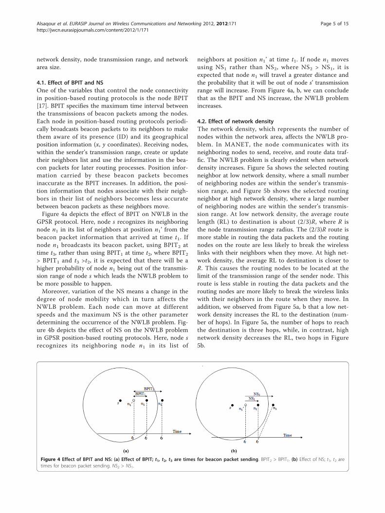
4.1. Effect of BPIT and NSOne of the variables that control the node connectivityin position-based routing protocols is the node BPIT[17]. BPIT specifies the maximum time interval betweenthe transmissions of beacon packets among the nodes.Each node in position-based routing protocols periodi-cally broadcasts beacon packets to its neighbors to makethem aware of its presence (ID) and its geographicalposition information (x, y coordinates). Receiving nodes,within the sender’s transmission range, create or updatetheir neighbors list and use the information in the bea-con packets for later routing processes. Position infor-mation carried by these beacon packets becomesinaccurate as the BPIT increases. In addition, the posi-tion information that nodes associate with their neigh-bors in their list of neighbors becomes less accuratebetween beacon packets as these neighbors move.Figure 4a depicts the effect of BPIT on NWLB in the

GPSR protocol. Here, node s recognizes its neighboringnode n1 in its list of neighbors at position n1’ from thebeacon packet information that arrived at time t1. Ifnode n1 broadcasts its beacon packet, using BPIT2 attime t3, rather than using BPIT1 at time t2, where BPIT2

> BPIT1 and t3 >t2, it is expected that there will be ahigher probability of node n1 being out of the transmis-sion range of node s which leads the NWLB problem tobe more possible to happen.Moreover, variation of the NS means a change in the

degree of node mobility which in turn affects theNWLB problem. Each node can move at differentspeeds and the maximum NS is the other parameterdetermining the occurrence of the NWLB problem. Fig-ure 4b depicts the effect of NS on the NWLB problemin GPSR position-based routing protocols. Here, node srecognizes its neighboring node n1 in its list of

neighbors at position n1’ at time t1. If node n1 movesusing NS1 rather than NS2, where NS2 > NS1, it isexpected that node n1 will travel a greater distance andthe probability that it will be out of node s’ transmissionrange will increase. From Figure 4a, b, we can concludethat as the BPIT and NS increase, the NWLB problemincreases.

4.2. Effect of network densityThe network density, which represents the number ofnodes within the network area, affects the NWLB pro-blem. In MANET, the node communicates with itsneighboring nodes to send, receive, and route data traf-fic. The NWLB problem is clearly evident when networkdensity increases. Figure 5a shows the selected routingneighbor at low network density, where a small numberof neighboring nodes are within the sender’s transmis-sion range, and Figure 5b shows the selected routingneighbor at high network density, where a large numberof neighboring nodes are within the sender’s transmis-sion range. At low network density, the average routelength (RL) to destination is about (2/3)R, where R isthe node transmission range radius. The (2/3)R route ismore stable in routing the data packets and the routingnodes on the route are less likely to break the wirelesslinks with their neighbors when they move. At high net-work density, the average RL to destination is closer toR. This causes the routing nodes to be located at thelimit of the transmission range of the sender node. Thisroute is less stable in routing the data packets and therouting nodes are more likely to break the wireless linkswith their neighbors in the route when they move. Inaddition, we observed from Figure 5a, b that a low net-work density increases the RL to the destination (num-ber of hops). In Figure 5a, the number of hops to reachthe destination is three hops, while, in contrast, highnetwork density decreases the RL, two hops in Figure5b.

Figure 4 Effect of BPIT and NS: (a) Effect of BPIT; t1, t2, t3 are times for beacon packet sending. BPIT2 > BPIT1. (b) Effect of NS; t1, t2 aretimes for beacon packet sending. NS2 > NS1.


Page 5 of 15

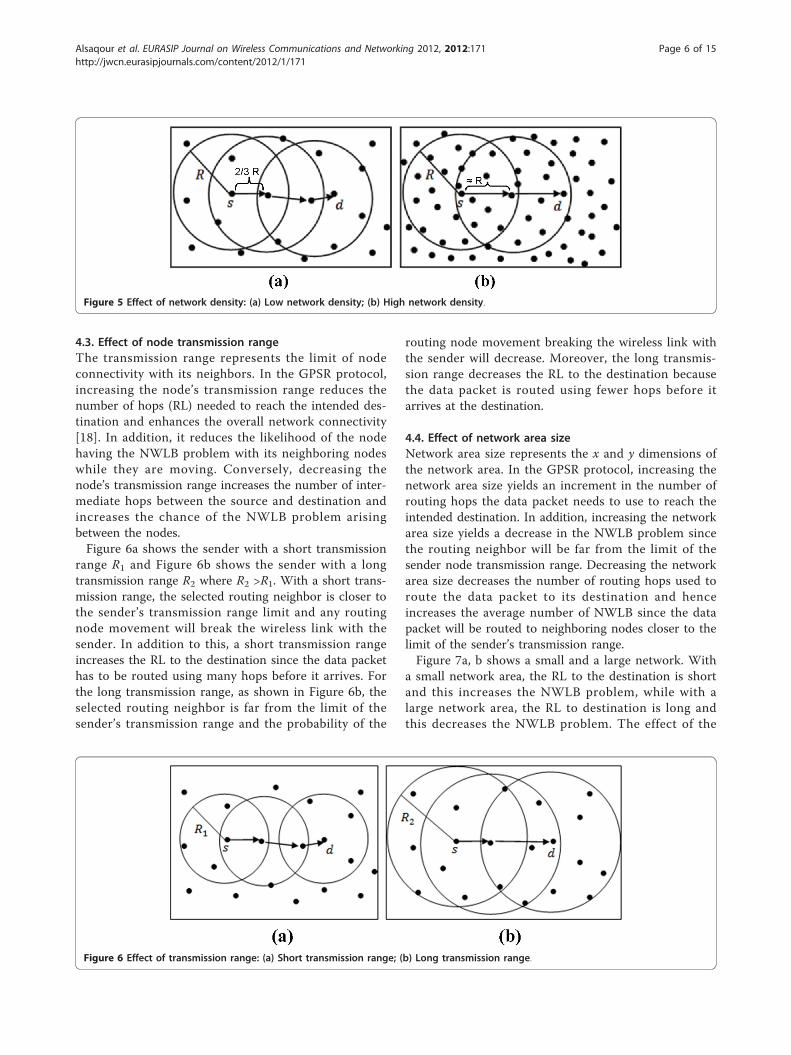
4.3. Effect of node transmission rangeThe transmission range represents the limit of nodeconnectivity with its neighbors. In the GPSR protocol,increasing the node’s transmission range reduces thenumber of hops (RL) needed to reach the intended des-tination and enhances the overall network connectivity[18]. In addition, it reduces the likelihood of the nodehaving the NWLB problem with its neighboring nodeswhile they are moving. Conversely, decreasing thenode’s transmission range increases the number of inter-mediate hops between the source and destination andincreases the chance of the NWLB problem arisingbetween the nodes.Figure 6a shows the sender with a short transmission

range R1 and Figure 6b shows the sender with a longtransmission range R2 where R2 >R1. With a short trans-mission range, the selected routing neighbor is closer tothe sender’s transmission range limit and any routingnode movement will break the wireless link with thesender. In addition to this, a short transmission rangeincreases the RL to the destination since the data packethas to be routed using many hops before it arrives. Forthe long transmission range, as shown in Figure 6b, theselected routing neighbor is far from the limit of thesender’s transmission range and the probability of the

routing node movement breaking the wireless link withthe sender will decrease. Moreover, the long transmis-sion range decreases the RL to the destination becausethe data packet is routed using fewer hops before itarrives at the destination.

4.4. Effect of network area sizeNetwork area size represents the x and y dimensions ofthe network area. In the GPSR protocol, increasing thenetwork area size yields an increment in the number ofrouting hops the data packet needs to use to reach theintended destination. In addition, increasing the networkarea size yields a decrease in the NWLB problem sincethe routing neighbor will be far from the limit of thesender node transmission range. Decreasing the networkarea size decreases the number of routing hops used toroute the data packet to its destination and henceincreases the average number of NWLB since the datapacket will be routed to neighboring nodes closer to thelimit of the sender’s transmission range.Figure 7a, b shows a small and a large network. With

a small network area, the RL to the destination is shortand this increases the NWLB problem, while with alarge network area, the RL to destination is long andthis decreases the NWLB problem. The effect of the

Figure 5 Effect of network density: (a) Low network density; (b) High network density.

Figure 6 Effect of transmission range: (a) Short transmission range; (b) Long transmission range.


Page 6 of 15

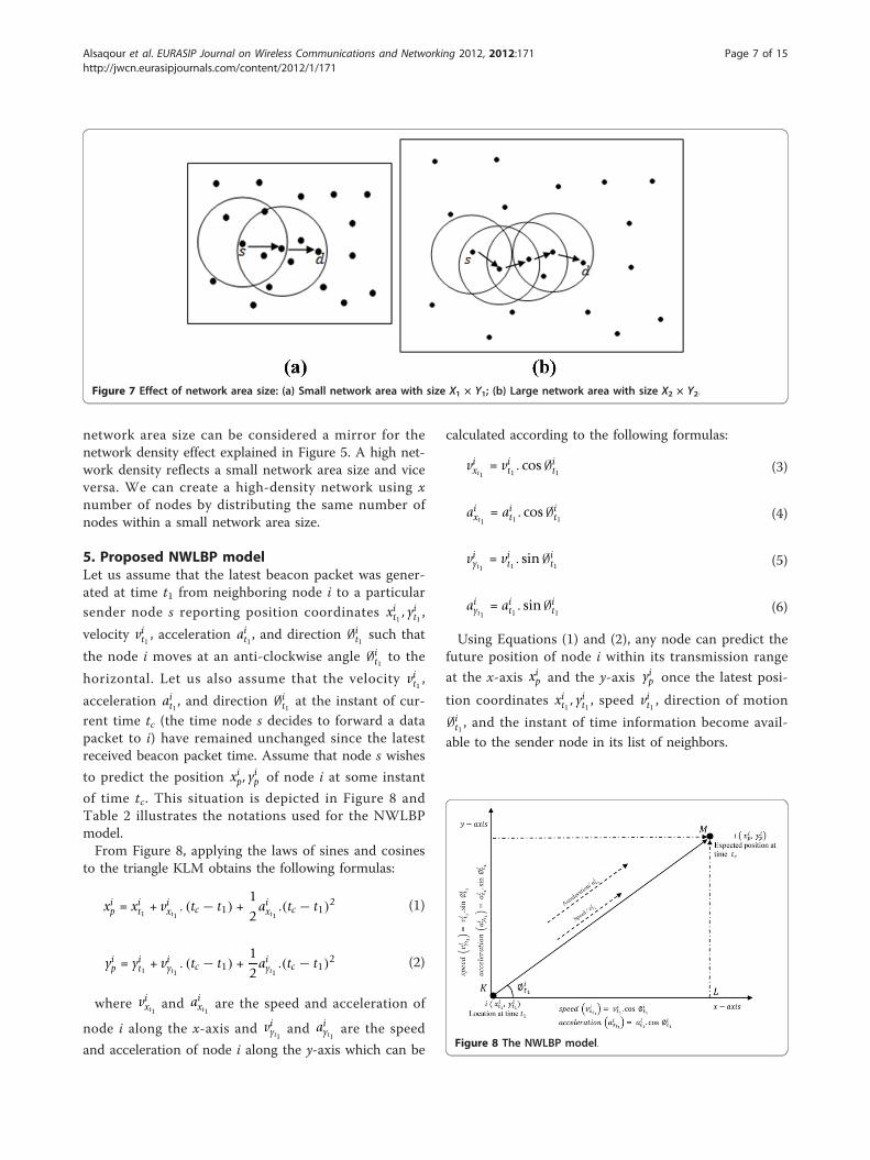
network area size can be considered a mirror for thenetwork density effect explained in Figure 5. A high net-work density reflects a small network area size and viceversa. We can create a high-density network using xnumber of nodes by distributing the same number ofnodes within a small network area size.

5. Proposed NWLBP modelLet us assume that the latest beacon packet was gener-ated at time t1 from neighboring node i to a particularsender node s reporting position coordinates xit1 , y

it1 ,

velocity vit1 , acceleration ait1 , and direction ∅it1 such that

the node i moves at an anti-clockwise angle ∅it1 to the

horizontal. Let us also assume that the velocity vit1 ,

acceleration ait1 , and direction ∅it1 at the instant of cur-

rent time tc (the time node s decides to forward a datapacket to i) have remained unchanged since the latestreceived beacon packet time. Assume that node s wishes

to predict the position xip, yip of node i at some instant

of time tc. This situation is depicted in Figure 8 andTable 2 illustrates the notations used for the NWLBPmodel.From Figure 8, applying the laws of sines and cosines

to the triangle KLM obtains the following formulas:

xip = xit1 + vixt1 . (tc − t1) +12aixt1 .(tc − t1)2 (1)

yip = yit1 + viyt1 . (tc − t1) +12aiyt1 .(tc − t1)2 (2)

where vixt1 and aixt1 are the speed and acceleration of

node i along the x-axis and viyt1 and aiyt1 are the speed

and acceleration of node i along the y-axis which can be

calculated according to the following formulas:

vixt1 = vit1 . cos ∅it1 (3)

aixt1 = ait1 . cos ∅it1 (4)

viyt1 = vit1 . sin ∅it1 (5)

aiyt1 = ait1 . sin ∅it1 (6)

Using Equations (1) and (2), any node can predict thefuture position of node i within its transmission range

at the x-axis xip and the y-axis yip once the latest posi-

tion coordinates xit1 , yit1 , speed vit1 , direction of motion

∅it1 , and the instant of time information become avail-

able to the sender node in its list of neighbors.

Figure 7 Effect of network area size: (a) Small network area with size X1 × Y1; (b) Large network area with size X2 × Y2.

Figure 8 The NWLBP model.


Page 7 of 15

To implement the proposed NWLBP model, thenodes need to record additional position informationabout its neighboring nodes in their lists of neighbors.For each neighbor, the following additional data arestored: the position coordinates xit1 , y

it1 , the speed vit1 ,

the acceleration ait1 , the direction ∅it1 along the x-axis,

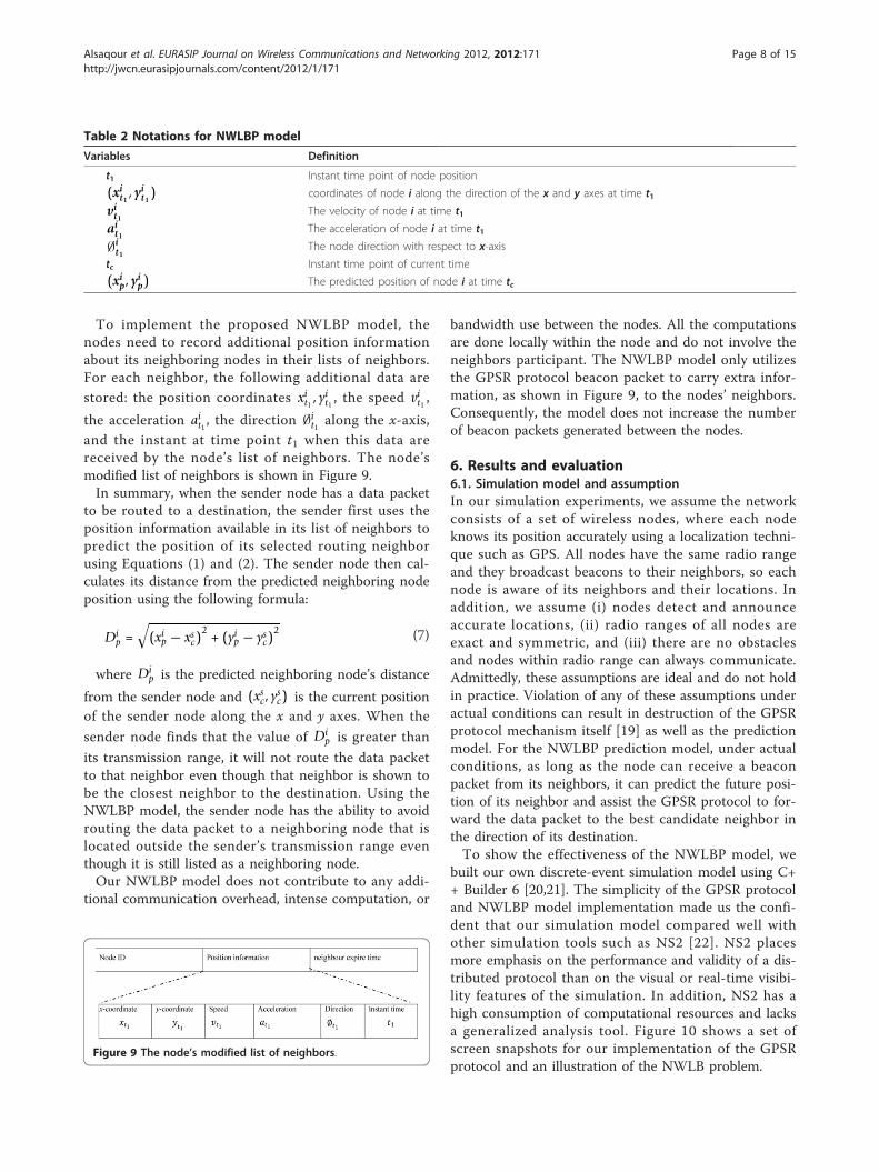
and the instant at time point t1 when this data arereceived by the node’s list of neighbors. The node’smodified list of neighbors is shown in Figure 9.In summary, when the sender node has a data packet

to be routed to a destination, the sender first uses theposition information available in its list of neighbors topredict the position of its selected routing neighborusing Equations (1) and (2). The sender node then cal-culates its distance from the predicted neighboring nodeposition using the following formula:

Dip =

√(xip − xsc)

2+ (yip − ysc)

2 (7)

where Dip is the predicted neighboring node’s distance

from the sender node and (xsc, ysc) is the current position

of the sender node along the x and y axes. When the

sender node finds that the value of Dip is greater than

its transmission range, it will not route the data packetto that neighbor even though that neighbor is shown tobe the closest neighbor to the destination. Using theNWLBP model, the sender node has the ability to avoidrouting the data packet to a neighboring node that islocated outside the sender’s transmission range eventhough it is still listed as a neighboring node.Our NWLBP model does not contribute to any addi-

tional communication overhead, intense computation, or

bandwidth use between the nodes. All the computationsare done locally within the node and do not involve theneighbors participant. The NWLBP model only utilizesthe GPSR protocol beacon packet to carry extra infor-mation, as shown in Figure 9, to the nodes’ neighbors.Consequently, the model does not increase the numberof beacon packets generated between the nodes.

6. Results and evaluation6.1. Simulation model and assumptionIn our simulation experiments, we assume the networkconsists of a set of wireless nodes, where each nodeknows its position accurately using a localization techni-que such as GPS. All nodes have the same radio rangeand they broadcast beacons to their neighbors, so eachnode is aware of its neighbors and their locations. Inaddition, we assume (i) nodes detect and announceaccurate locations, (ii) radio ranges of all nodes areexact and symmetric, and (iii) there are no obstaclesand nodes within radio range can always communicate.Admittedly, these assumptions are ideal and do not holdin practice. Violation of any of these assumptions underactual conditions can result in destruction of the GPSRprotocol mechanism itself [19] as well as the predictionmodel. For the NWLBP prediction model, under actualconditions, as long as the node can receive a beaconpacket from its neighbors, it can predict the future posi-tion of its neighbor and assist the GPSR protocol to for-ward the data packet to the best candidate neighbor inthe direction of its destination.To show the effectiveness of the NWLBP model, we

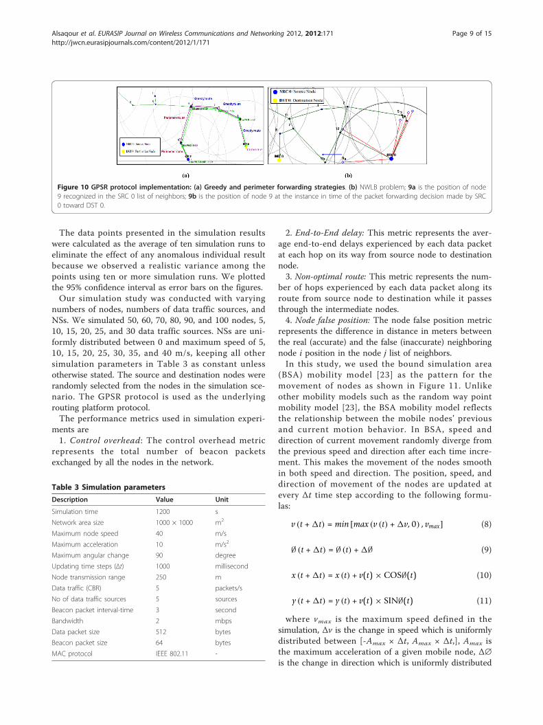
built our own discrete-event simulation model using C++ Builder 6 [20,21]. The simplicity of the GPSR protocoland NWLBP model implementation made us the confi-dent that our simulation model compared well withother simulation tools such as NS2 [22]. NS2 placesmore emphasis on the performance and validity of a dis-tributed protocol than on the visual or real-time visibi-lity features of the simulation. In addition, NS2 has ahigh consumption of computational resources and lacksa generalized analysis tool. Figure 10 shows a set ofscreen snapshots for our implementation of the GPSRprotocol and an illustration of the NWLB problem.

Table 2 Notations for NWLBP model

Variables Definition

t1 Instant time point of node position

(xit1 , yit1) coordinates of node i along the direction of the x and y axes at time t1

vit1 The velocity of node i at time t1ait1 The acceleration of node i at time t1

∅it1

The node direction with respect to x-axis

tc Instant time point of current time

(xip, yip) The predicted position of node i at time tc

Figure 9 The node’s modified list of neighbors.


Page 8 of 15

The data points presented in the simulation resultswere calculated as the average of ten simulation runs toeliminate the effect of any anomalous individual resultbecause we observed a realistic variance among thepoints using ten or more simulation runs. We plottedthe 95% confidence interval as error bars on the figures.Our simulation study was conducted with varying

numbers of nodes, numbers of data traffic sources, andNSs. We simulated 50, 60, 70, 80, 90, and 100 nodes, 5,10, 15, 20, 25, and 30 data traffic sources. NSs are uni-formly distributed between 0 and maximum speed of 5,10, 15, 20, 25, 30, 35, and 40 m/s, keeping all othersimulation parameters in Table 3 as constant unlessotherwise stated. The source and destination nodes wererandomly selected from the nodes in the simulation sce-nario. The GPSR protocol is used as the underlyingrouting platform protocol.The performance metrics used in simulation experi-

ments are1. Control overhead: The control overhead metric

represents the total number of beacon packetsexchanged by all the nodes in the network.

2. End-to-End delay: This metric represents the aver-age end-to-end delays experienced by each data packetat each hop on its way from source node to destinationnode.3. Non-optimal route: This metric represents the num-

ber of hops experienced by each data packet along itsroute from source node to destination while it passesthrough the intermediate nodes.4. Node false position: The node false position metric

represents the difference in distance in meters betweenthe real (accurate) and the false (inaccurate) neighboringnode i position in the node j list of neighbors.In this study, we used the bound simulation area

(BSA) mobility model [23] as the pattern for themovement of nodes as shown in Figure 11. Unlikeother mobility models such as the random way pointmobility model [23], the BSA mobility model reflectsthe relationship between the mobile nodes’ previousand current motion behavior. In BSA, speed anddirection of current movement randomly diverge fromthe previous speed and direction after each time incre-ment. This makes the movement of the nodes smoothin both speed and direction. The position, speed, anddirection of movement of the nodes are updated atevery Δt time step according to the following formu-las:

v (t + �t) = min [max (v (t) + �v, 0) , vmax] (8)

∅ (t + �t) = ∅ (t) + �∅ (9)

x (t + �t) = x (t) + v(t) × COS∅(t) (10)

y (t + �t) = y (t) + v(t) × SIN∅(t) (11)

where vmax is the maximum speed defined in thesimulation, Δv is the change in speed which is uniformlydistributed between [-Amax × Δt, Amax × Δt,], Amax isthe maximum acceleration of a given mobile node, Δ∅is the change in direction which is uniformly distributed

Figure 10 GPSR protocol implementation: (a) Greedy and perimeter forwarding strategies. (b) NWLB problem; 9a is the position of node9 recognized in the SRC 0 list of neighbors; 9b is the position of node 9 at the instance in time of the packet forwarding decision made by SRC0 toward DST 0.

Table 3 Simulation parameters

Description Value Unit

Simulation time 1200 s

Network area size 1000 × 1000 m2

Maximum node speed 40 m/s

Maximum acceleration 10 m/s2

Maximum angular change 90 degree

Updating time steps (Δt) 1000 millisecond

Node transmission range 250 m

Data traffic (CBR) 5 packets/s

No of data traffic sources 5 sources

Beacon packet interval-time 3 second

Bandwidth 2 mbps

Data packet size 512 bytes

Beacon packet size 64 bytes

MAC protocol IEEE 802.11 -


Page 9 of 15

between [-∞ × Δt, ∞ × Δt], and ∞ is the maximumangular change in the direction of mobile node travel.

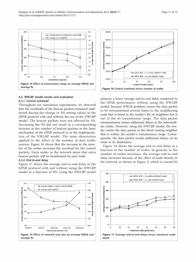
6.2. Effect of network parameters on the NWLB problemFigure 12 shows the effect of BPIT and NS on theoccurrence of the NWLB problem in the GPSR protocolfor different BPIT and NS values. As the BPIT and NSincrease, the percentage of neighbors who break thewireless link with the sender also increases. LongerBPIT and a high NS yield results in neighbors beinglisted in the sender’s list of neighbors when they are infact outside the transmission range as shown in Figure4.Figure 13 shows the effect of network density on the

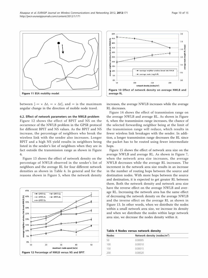
percentage of NWLB observed in the sender’s list ofneighbors and the average RL for four different networkdensities as shown in Table 4. In general and for thereasons shown in Figure 5, when the network density

increases, the average NWLB increases while the averageRL decreases.Figure 14 shows the effect of transmission range on

the average NWLB and average RL. As shown in Figure6, when the transmission range increases, the chance ofthe selected forwarding neighbor being at the limit ofthe transmission range will reduce, which results infewer wireless link breakages with the sender. In addi-tion, a longer transmission range decreases the RL sincethe packet has to be routed using fewer intermediatehops.Figure 15 shows the effect of network area size on the

average NWLB and average RL. As shown in Figure 7,when the network area size increases, the averageNWLB decreases while the average RL increases. Theincrement in the network area size results in an increasein the number of routing hops between the source anddestination nodes. With more hops between the sourceand destination, it is expected to get greater RL betweenthem. Both the network density and network area sizehave the reverse effect on the average NWLB and aver-age RL. Increasing the network area has the same effectof decreasing the network density on the average NWLBand the inverse effect on the average RL as shown inFigure 13. In other words, when we distribute the nodeswithin a small network area size, we increase its densityand when we distribute the nodes within large networkarea size, we decrease the nodes density within it.

Figure 11 BSA mobility model.

Figure 12 Percentage of NWLB versus NS and BPIT.

Figure 13 Effect of network density on average NWLB andaverage RL.

Table 4 Nodes versus network density

Nodes Network density (nodes/m2)

50 0.00005

100 0.00010

150 0.00015

200 0.00020


Page 10 of 15

6.3. WNLBP model results and evaluation6.3.1. Control overheadThroughout our simulation experiments, we observedthat the overheads of the beacon packets remained unaf-fected during the change in NS setting values in theGPSR protocol with and without the use of the NWLBPmodel. The beacon packets were not affected by NS.Increasing the NS did not result in a correspondingincrease in the number of beacon packets in the basicmechanism of the GPSR protocol or in the implementa-tion of the NWLBP model. The same observationapplied to the effect of the number of data trafficsources. Figure 16 shows that the increase in the num-ber of the nodes increases the overhead for the controlpackets. Extra nodes in the network mean that extrabeacon packets will be broadcasted by each node.6.3.2. End-to-end delayFigure 17 shows the average end-to-end delay in theGPSR protocol with and without using the NWLBPmodel as a function of NS. Using the NWLBP model

achieves a lower average end-to-end delay compared tothe GPSR performance without using the NWLBPmodel, because NWLB problem causes the data packetto be retransmitted several times to the neighboringnode that is listed in the sender’s list of neighbors but isout of the its transmission range. The data packetretransmission causes additional delays at the intermedi-ate nodes. However, using the NWLBP model, the sen-der routes the data packet to the listed routing neighborthat is within the sender’s transmission range. Conse-quently, the data packet avoids additional delays on itsroute to its destination.Figure 18 shows the average end-to-end delay as a

function of the number of nodes. In general, as thenumber of nodes increases, the average end-to-enddelay increases because of the effect of node density inthe network as shown in Figure 5, which is caused by

Figure 14 Effect of transmission range on average NWLB andaverage RL.

Figure 15 Effect of network area size on average NWLB andaverage RL.

Figure 16 Control overhead versus number of nodes.

Figure 17 Average end-to-end delay versus maximum nodespeed.


Page 11 of 15

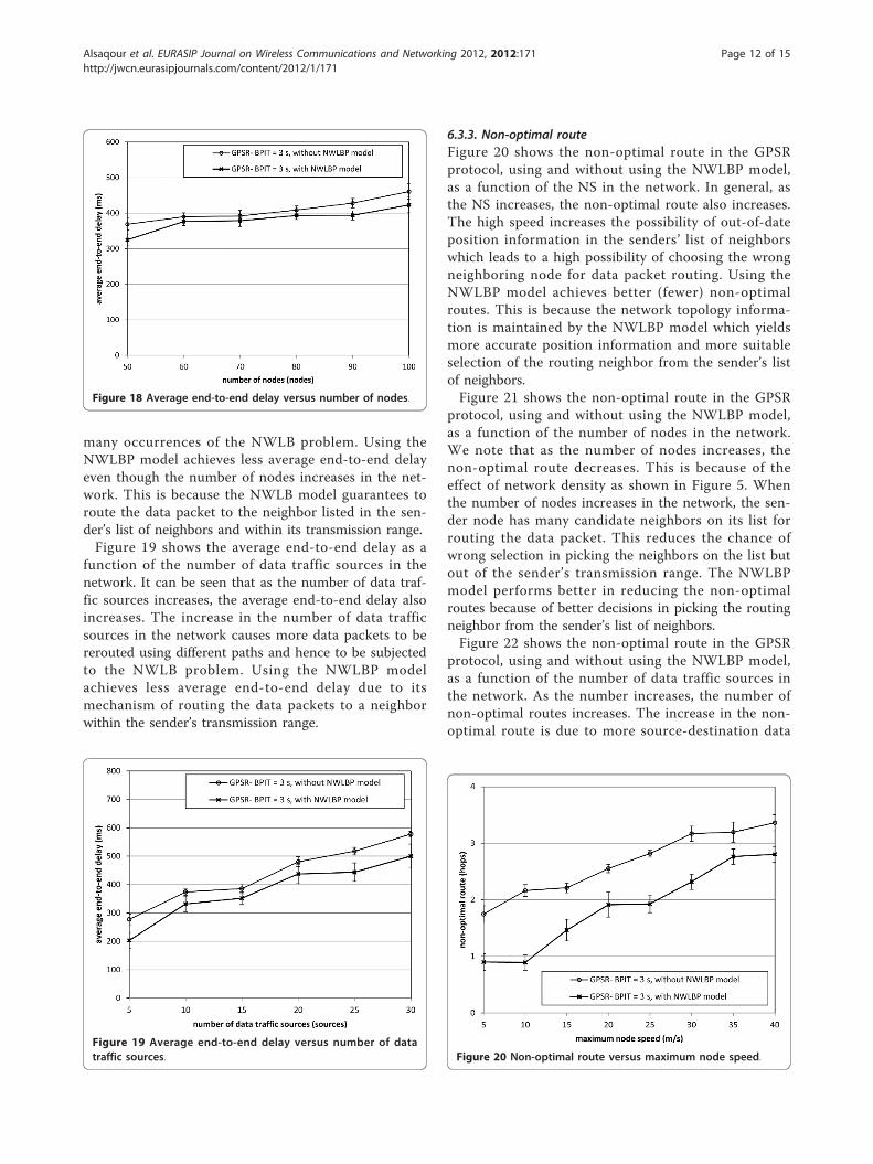
many occurrences of the NWLB problem. Using theNWLBP model achieves less average end-to-end delayeven though the number of nodes increases in the net-work. This is because the NWLB model guarantees toroute the data packet to the neighbor listed in the sen-der’s list of neighbors and within its transmission range.Figure 19 shows the average end-to-end delay as a

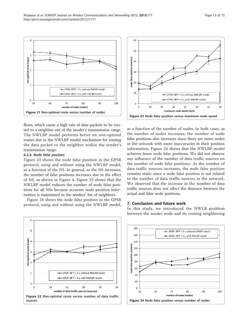
function of the number of data traffic sources in thenetwork. It can be seen that as the number of data traf-fic sources increases, the average end-to-end delay alsoincreases. The increase in the number of data trafficsources in the network causes more data packets to bererouted using different paths and hence to be subjectedto the NWLB problem. Using the NWLBP modelachieves less average end-to-end delay due to itsmechanism of routing the data packets to a neighborwithin the sender’s transmission range.

6.3.3. Non-optimal routeFigure 20 shows the non-optimal route in the GPSRprotocol, using and without using the NWLBP model,as a function of the NS in the network. In general, asthe NS increases, the non-optimal route also increases.The high speed increases the possibility of out-of-dateposition information in the senders’ list of neighborswhich leads to a high possibility of choosing the wrongneighboring node for data packet routing. Using theNWLBP model achieves better (fewer) non-optimalroutes. This is because the network topology informa-tion is maintained by the NWLBP model which yieldsmore accurate position information and more suitableselection of the routing neighbor from the sender’s listof neighbors.Figure 21 shows the non-optimal route in the GPSR

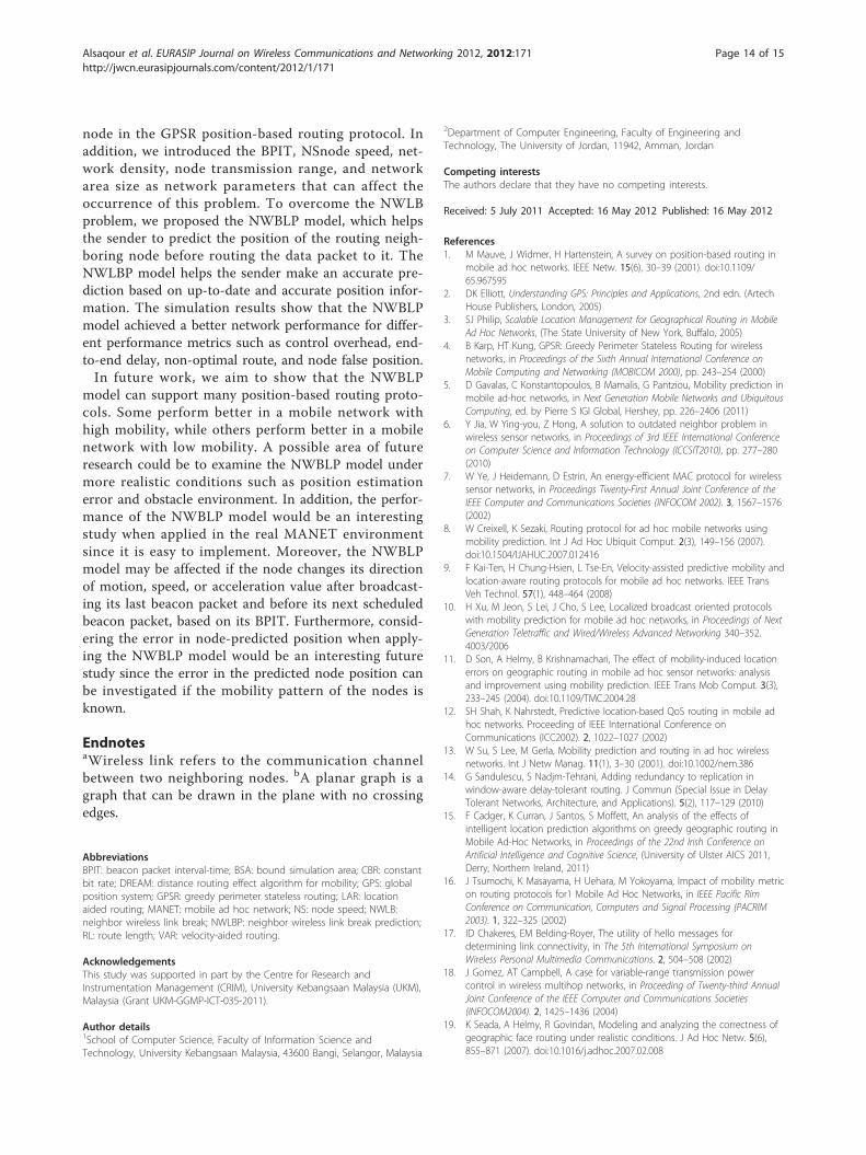
protocol, using and without using the NWLBP model,as a function of the number of nodes in the network.We note that as the number of nodes increases, thenon-optimal route decreases. This is because of theeffect of network density as shown in Figure 5. Whenthe number of nodes increases in the network, the sen-der node has many candidate neighbors on its list forrouting the data packet. This reduces the chance ofwrong selection in picking the neighbors on the list butout of the sender’s transmission range. The NWLBPmodel performs better in reducing the non-optimalroutes because of better decisions in picking the routingneighbor from the sender’s list of neighbors.Figure 22 shows the non-optimal route in the GPSR

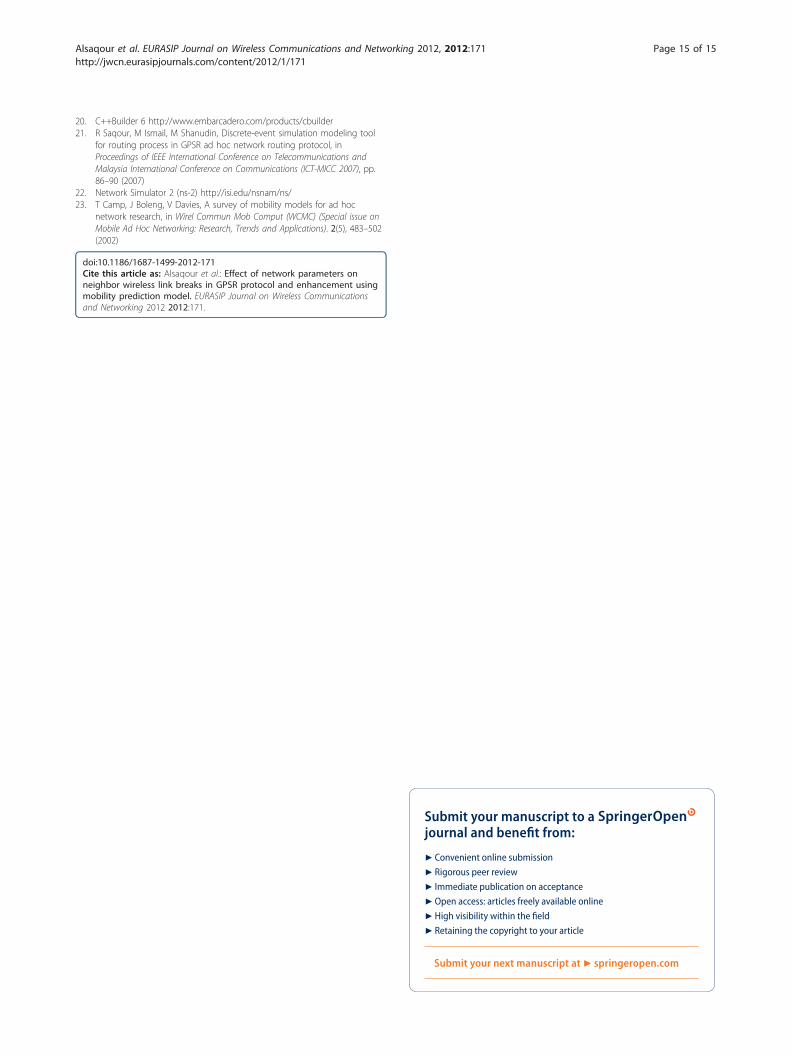
protocol, using and without using the NWLBP model,as a function of the number of data traffic sources inthe network. As the number increases, the number ofnon-optimal routes increases. The increase in the non-optimal route is due to more source-destination data

Figure 18 Average end-to-end delay versus number of nodes.

Figure 19 Average end-to-end delay versus number of datatraffic sources. Figure 20 Non-optimal route versus maximum node speed.


Page 12 of 15

flows, which cause a high rate of data packets to be rou-ted to a neighbor out of the sender’s transmission range.The NWLBP model performs better on non-optimalroutes due to the NWLBP model mechanism for routingthe data packet to the neighbor within the sender’stransmission range.6.3.4. Node false positionFigure 23 shows the node false position in the GPSRprotocol, using and without using the NWLBP model,as a function of the NS. In general, as the NS increases,the number of false positions increases due to the effectof NS, as shown in Figure 4. Figure 23 shows that theNWLBP model reduces the number of node false posi-tions for all NSs because accurate node position infor-mation is maintained in the senders’ list of neighbors.Figure 24 shows the node false position in the GPSR

protocol, using and without using the NWLBP model,

as a function of the number of nodes. In both cases, asthe number of nodes increases, the number of nodefalse positions also increases since there are more nodesin the network with more inaccuracies in their positioninformation. Figure 24 shows that the NWLBP modelachieves fewer node false positions. We did not observeany influence of the number of data traffic sources onthe number of node false positions. As the number ofdata traffic sources increases, the node false positionremains static since a node false position is not relatedto the number of data traffic sources in the network.We observed that the increase in the number of datatraffic sources does not affect the distance between theactual and false node positions.

7. Conclusion and future workIn this study, we introduced the NWLB problembetween the sender node and its routing neighboring

Figure 21 Non-optimal route versus number of nodes.

Figure 22 Non-optimal route versus number of data trafficsources.

Figure 23 Node false position versus maximum node speed.

Figure 24 Node false position versus number of nodes.


Page 13 of 15

node in the GPSR position-based routing protocol. Inaddition, we introduced the BPIT, NSnode speed, net-work density, node transmission range, and networkarea size as network parameters that can affect theoccurrence of this problem. To overcome the NWLBproblem, we proposed the NWBLP model, which helpsthe sender to predict the position of the routing neigh-boring node before routing the data packet to it. TheNWLBP model helps the sender make an accurate pre-diction based on up-to-date and accurate position infor-mation. The simulation results show that the NWBLPmodel achieved a better network performance for differ-ent performance metrics such as control overhead, end-to-end delay, non-optimal route, and node false position.In future work, we aim to show that the NWBLP

model can support many position-based routing proto-cols. Some perform better in a mobile network withhigh mobility, while others perform better in a mobilenetwork with low mobility. A possible area of futureresearch could be to examine the NWBLP model undermore realistic conditions such as position estimationerror and obstacle environment. In addition, the perfor-mance of the NWBLP model would be an interestingstudy when applied in the real MANET environmentsince it is easy to implement. Moreover, the NWBLPmodel may be affected if the node changes its directionof motion, speed, or acceleration value after broadcast-ing its last beacon packet and before its next scheduledbeacon packet, based on its BPIT. Furthermore, consid-ering the error in node-predicted position when apply-ing the NWBLP model would be an interesting futurestudy since the error in the predicted node position canbe investigated if the mobility pattern of the nodes isknown.

EndnotesaWireless link refers to the communication channelbetween two neighboring nodes. bA planar graph is agraph that can be drawn in the plane with no crossingedges.

AbbreviationsBPIT: beacon packet interval-time; BSA: bound simulation area; CBR: constantbit rate; DREAM: distance routing effect algorithm for mobility; GPS: globalposition system; GPSR: greedy perimeter stateless routing; LAR: locationaided routing; MANET: mobile ad hoc network; NS: node speed; NWLB:neighbor wireless link break; NWLBP: neighbor wireless link break prediction;RL: route length; VAR: velocity-aided routing.

AcknowledgementsThis study was supported in part by the Centre for Research andInstrumentation Management (CRIM), University Kebangsaan Malaysia (UKM),Malaysia (Grant UKM-GGMP-ICT-035-2011).

Author details1School of Computer Science, Faculty of Information Science andTechnology, University Kebangsaan Malaysia, 43600 Bangi, Selangor, Malaysia

2Department of Computer Engineering, Faculty of Engineering andTechnology, The University of Jordan, 11942, Amman, Jordan

Competing interestsThe authors declare that they have no competing interests.

Received: 5 July 2011 Accepted: 16 May 2012 Published: 16 May 2012

References1. M Mauve, J Widmer, H Hartenstein, A survey on position-based routing in

mobile ad hoc networks. IEEE Netw. 15(6), 30–39 (2001). doi:10.1109/65.967595

2. DK Elliott, Understanding GPS: Principles and Applications, 2nd edn. (ArtechHouse Publishers, London, 2005)

3. SJ Philip, Scalable Location Management for Geographical Routing in MobileAd Hoc Networks, (The State University of New York, Buffalo, 2005)

4. B Karp, HT Kung, GPSR: Greedy Perimeter Stateless Routing for wirelessnetworks, in Proceedings of the Sixth Annual International Conference onMobile Computing and Networking (MOBICOM 2000), pp. 243–254 (2000)

5. D Gavalas, C Konstantopoulos, B Mamalis, G Pantziou, Mobility prediction inmobile ad-hoc networks, in Next Generation Mobile Networks and UbiquitousComputing, ed. by Pierre S IGI Global, Hershey, pp. 226–2406 (2011)

6. Y Jia, W Ying-you, Z Hong, A solution to outdated neighbor problem inwireless sensor networks, in Proceedings of 3rd IEEE International Conferenceon Computer Science and Information Technology (ICCSIT2010), pp. 277–280(2010)

7. W Ye, J Heidemann, D Estrin, An energy-efficient MAC protocol for wirelesssensor networks, in Proceedings Twenty-First Annual Joint Conference of theIEEE Computer and Communications Societies (INFOCOM 2002). 3, 1567–1576(2002)

8. W Creixell, K Sezaki, Routing protocol for ad hoc mobile networks usingmobility prediction. Int J Ad Hoc Ubiquit Comput. 2(3), 149–156 (2007).doi:10.1504/IJAHUC.2007.012416

9. F Kai-Ten, H Chung-Hsien, L Tse-En, Velocity-assisted predictive mobility andlocation-aware routing protocols for mobile ad hoc networks. IEEE TransVeh Technol. 57(1), 448–464 (2008)

10. H Xu, M Jeon, S Lei, J Cho, S Lee, Localized broadcast oriented protocolswith mobility prediction for mobile ad hoc networks, in Proceedings of NextGeneration Teletraffic and Wired/Wireless Advanced Networking 340–352.4003/2006

11. D Son, A Helmy, B Krishnamachari, The effect of mobility-induced locationerrors on geographic routing in mobile ad hoc sensor networks: analysisand improvement using mobility prediction. IEEE Trans Mob Comput. 3(3),233–245 (2004). doi:10.1109/TMC.2004.28

12. SH Shah, K Nahrstedt, Predictive location-based QoS routing in mobile adhoc networks. Proceeding of IEEE International Conference onCommunications (ICC2002). 2, 1022–1027 (2002)

13. W Su, S Lee, M Gerla, Mobility prediction and routing in ad hoc wirelessnetworks. Int J Netw Manag. 11(1), 3–30 (2001). doi:10.1002/nem.386

14. G Sandulescu, S Nadjm-Tehrani, Adding redundancy to replication inwindow-aware delay-tolerant routing. J Commun (Special Issue in DelayTolerant Networks, Architecture, and Applications). 5(2), 117–129 (2010)

15. F Cadger, K Curran, J Santos, S Moffett, An analysis of the effects ofintelligent location prediction algorithms on greedy geographic routing inMobile Ad-Hoc Networks, in Proceedings of the 22nd Irish Conference onArtificial Intelligence and Cognitive Science, (University of Ulster AICS 2011,Derry, Northern Ireland, 2011)

16. J Tsumochi, K Masayama, H Uehara, M Yokoyama, Impact of mobility metricon routing protocols for1 Mobile Ad Hoc Networks, in IEEE Pacific RimConference on Communication, Computers and Signal Processing (PACRIM2003). 1, 322–325 (2002)

17. ID Chakeres, EM Belding-Royer, The utility of hello messages fordetermining link connectivity, in The 5th International Symposium onWireless Personal Multimedia Communications. 2, 504–508 (2002)

18. J Gomez, AT Campbell, A case for variable-range transmission powercontrol in wireless multihop networks, in Proceeding of Twenty-third AnnualJoint Conference of the IEEE Computer and Communications Societies(INFOCOM2004). 2, 1425–1436 (2004)

19. K Seada, A Helmy, R Govindan, Modeling and analyzing the correctness ofgeographic face routing under realistic conditions. J Ad Hoc Netw. 5(6),855–871 (2007). doi:10.1016/j.adhoc.2007.02.008


Page 14 of 15

20. C++Builder 6 http://www.embarcadero.com/products/cbuilder21. R Saqour, M Ismail, M Shanudin, Discrete-event simulation modeling tool

for routing process in GPSR ad hoc network routing protocol, inProceedings of IEEE International Conference on Telecommunications andMalaysia International Conference on Communications (ICT-MICC 2007), pp.86–90 (2007)

22. Network Simulator 2 (ns-2) http://isi.edu/nsnam/ns/23. T Camp, J Boleng, V Davies, A survey of mobility models for ad hoc

network research, in Wirel Commun Mob Comput (WCMC) (Special issue onMobile Ad Hoc Networking: Research, Trends and Applications). 2(5), 483–502(2002)

doi:10.1186/1687-1499-2012-171Cite this article as: Alsaqour et al.: Effect of network parameters onneighbor wireless link breaks in GPSR protocol and enhancement usingmobility prediction model. EURASIP Journal on Wireless Communicationsand Networking 2012 2012:171.

Submit your manuscript to a journal and benefi t from:

7 Convenient online submission

7 Rigorous peer review

7 Immediate publication on acceptance

7 Open access: articles freely available online

7 High visibility within the fi eld

7 Retaining the copyright to your article

Submit your next manuscript at 7 springeropen.com


Page 15 of 15

http://www.embarcadero.com/products/cbuilder

http://isi.edu/nsnam/ns/

http://www.springeropen.com/

http://www.springeropen.com/

Documents

RESEARCH Open Access Effect of network parameters on