FP6-NEST-PATH project no: 29085Report Version: 1

Report Preparation Date: July 07, 2008Classication: Pub.Deliverable no. 5.1

Closing the Loop of Sound Evaluation andDesign (CLOSED)

Deliverable 5.1

Representations and Predictors forEveryday Sounds

Kamil Adiloglu, Robert Annies,Hendrik Purwins, Klaus Obermayer

Neural Information Processing Group (NIPG)School IV – Electrical engineering and Computer Science

Technische Unversitat Berlin

2

Contents

1 Introduction 6

2 General framework 82.1 Perception and Recognition of Sound . . . . . . . . . . . . . . . . . . . . . 82.2 Predictors as Human Perception/Recognition Model . . . . . . . . . . . . 10

2.2.1 Prediction . . . . . . . . . . . . . . . . . . . . . . . . . . . . . . . . 102.2.2 Representation . . . . . . . . . . . . . . . . . . . . . . . . . . . . . 102.2.3 Classification . . . . . . . . . . . . . . . . . . . . . . . . . . . . . . 122.2.4 Learning . . . . . . . . . . . . . . . . . . . . . . . . . . . . . . . . . 15

3 Classification of Sound 183.1 Representations . . . . . . . . . . . . . . . . . . . . . . . . . . . . . . . . . 18

3.1.1 Spike Coding of Audio Signals . . . . . . . . . . . . . . . . . . . . 193.1.2 Gammatone Filters based Representation . . . . . . . . . . . . . . 283.1.3 Other Representation Schemes . . . . . . . . . . . . . . . . . . . . 31

3.2 Evaluation . . . . . . . . . . . . . . . . . . . . . . . . . . . . . . . . . . . . 323.2.1 Spike Representation . . . . . . . . . . . . . . . . . . . . . . . . . . 323.2.2 Representation Comparison . . . . . . . . . . . . . . . . . . . . . . 343.2.3 Outlook: General Everyday-Sounds Classification . . . . . . . . . . 36

4 Case study: Impact Sounds 394.1 Perceptual control of Impact Sound Synthesis . . . . . . . . . . . . . . . . 39

4.1.1 Simulating Materials . . . . . . . . . . . . . . . . . . . . . . . . . . 394.1.2 Prediction of Material Classes . . . . . . . . . . . . . . . . . . . . . 414.1.3 Experiments . . . . . . . . . . . . . . . . . . . . . . . . . . . . . . 424.1.4 Results . . . . . . . . . . . . . . . . . . . . . . . . . . . . . . . . . 434.1.5 Discussion . . . . . . . . . . . . . . . . . . . . . . . . . . . . . . . . 43

4.2 Representation of Impact Sounds . . . . . . . . . . . . . . . . . . . . . . . 444.2.1 Results . . . . . . . . . . . . . . . . . . . . . . . . . . . . . . . . . 44

4.3 Conclusion . . . . . . . . . . . . . . . . . . . . . . . . . . . . . . . . . . . 454.4 Outlook: Preliminary Experiments with Timbre Descriptors . . . . . . . . 45

4.4.1 Car Horn Sounds . . . . . . . . . . . . . . . . . . . . . . . . . . . . 46

5 Alternative Approaches 495.1 Adaptive Bottle Experiment . . . . . . . . . . . . . . . . . . . . . . . . . . 49

5.1.1 Introduction . . . . . . . . . . . . . . . . . . . . . . . . . . . . . . 495.1.2 Adaptive Bottle Optimization . . . . . . . . . . . . . . . . . . . . . 50

3

6 Conclusion & Discussion 566.1 Representation . . . . . . . . . . . . . . . . . . . . . . . . . . . . . . . . . 566.2 Adaptive Optimization . . . . . . . . . . . . . . . . . . . . . . . . . . . . . 57

4

Notation

fraktur script (s,M, . . .) denote measures, quantities or functions in the domain of psy-chology, cognition or psychophysics. It denotes something that has to be modeledin order to make it mathematically tractable. Thus, there is only a qualitativedefinition.

bold letters (xi) denote vectors in Rn

italic letters (xi) scalar values

capital letters (M) sets, G = (V,E) denotes graphs, where V denotes the vertices andE denotes the edges.

bold capitals (T) matrices

indices (i,α) i, j, . . . index examples and the upper index α different contexts or models,

which is omitted where appropriate, yT denotes a target value, which is the knownlabel of an example x.

angle brackets inner/dot/scalar product: 〈x,y〉

5

1 Introduction

This report documents the work of NIPG within the CLOSED project according tothe tasks T5.1 and T5.2 defined in Workpackage 5: Measurement Definition. WithinCLOSED we have investigated what methods of machine learning, signal processing andstatistics are applicable to construct predictors for everyday sounds. These predictorscan be used in computer assisted sound design and in research on human perception andrecognition. This includes to find a suitable representation for everyday sounds.

The context of this research is the work of our partners, who provided their resultsas input to us. In particular we used the developed sound synthesis models in D2.1 [34]by UNIVERONA, D3.1 [51] on scenarios and interaction by ZHdK and the teoreticalwork in D4.1 [19] by IRCAM. This work was essential to us to work out an adequateframework and carry out the experiments on everyday sound classification.

Perception and classification of everyday sounds is a task, which human beings performeach day. In D4.1 was shown that the context and experience and the ability to categorizeplay an important role in perception and classification of everyday sounds. In D2.1 aneveryday sound taxonomy was proposed from a generating point of view. Depending onthis taxonomy UNIVERONA delivered the sound design tools in terms of physically-based sound synthesis algorithms. D3.1 influenced our work particularly in the researchof online sound adaptation of an artifact that incorporates human interaction.

In this deliverable, we present the psycho-acoustically relevant features in the classi-fication of the everyday sounds – with respect to the above sound taxonomy – and themethods we used to extract these features. Binary and multi-class classification experi-ments have been performed using different machine learning algorithms, in order to testthe performance of the representation methods.

The classification experiments can be performed by making use of a sound databaseprepared beforehand. However, in a psychoacoustical experiment, the sounds are pre-sented to the subjects online. In these kinds of experiments, subjects listen to the soundsrandomly, and evaluate them in an online fashion. Therefore, we have been working withIRCAM together on a new online experimental paradigm, which selects the sounds tobe presented to the subjects in a more clever way than random selection. The so-calledactive learning scenario has been adapted to perform psychoacoustical experiments.

Online learning proposes many possibilities not only in a classification scenario. Onlineclassifiers and predictors, based on psychoacoustically relevant features, which reducethe number of data points (sounds) to perform an experiment enables us to developoptimization algorithms for the sound design tools developed by UNIVERONA in WP2. These optimization algorithms are utilized in interactive scenarios and sound productsdeveloped by ZHdK in WP 3 used in psychoacoustical sound optimization experiments.In D4.2, IRCAM develops experimental methods to study the suitability of a sound

6

product for a function in these interaction scenarios. Consequently, online optimizationalgorithms can be incorporated to combine all these research studies to improve thequality of the sound design tools considering their support of the sound products in aninteractive experimental scenario.

In this report, the general frame work related to the theoretical work on perceptionis presented in Chapter 2. Chapter 3 documents the work on sound classifcation andrepresentation. A practical case study incorporating the sound design tools in an onlineexperimental paradigm is introduced in Chapter 4. Chapter 5 explains the details of theonline interactive optimization in another case study.

7

2 General framework

Perception of everyday sounds is an upcoming topic, which is in the focus of psychoa-coustical research as well as music and speech perception. Firstly to learn more aboutsound perception and recognition in natural and urban environments, secondly to gainknowledge of how to adapt sound generating processes of technical devices to supporttheir usability, design sounds for auditory displays or reflect or induce certain emotionsof the listener. To achieve this we need to analyze the relation between sound and humanrecognition and perception. Training predictors is a way to study this relationship andto develop measurement tools of perceptual parameters.

In a top-down approach the connection between an acoustic signal and perceptualcategories of sound events, sources or emotional responses is modeled. We will formal-ize the ideas mathematically as far as possible to make it tractable for computationalmethods, so that we are able to propose methods for sound design and analysis.

2.1 Perception and Recognition of Sound

The human perception of the world depends strongly on the ability to categorize. Inpsychophysics and cognition this research is generally summarized under the term cat-egorical perception. Research on grouping of colors [10], [3] and categorical perceptionof speech phonemes [26] show the principle, that the perception discretizes continuousstimuli, such that the discriminability within categories is small and between categoriesis large. Boundary effects appear [35], where perception jumps from one to anothercategory without effecting a perception of a continuous transition (e.g. between thephonemes /ka/ and /pa/).

Categorical perception theory addresses questions about the origin of categories. Arethey innate or learned and if yes, how are they learned? Are they induced by physi-cal/physiological facts or by cognitive decisions? Can boundaries be adapted by training?Why does categorical perception exist at all?

A thorough literature review was given in D4.1 of WP4 [19] section 1.2, which empha-sizes the importance of categories for human perception and recognition. It was discussedand concluded, – and this is the basis of D5.1 – that similarity and categorization arethe basic building blocks of perception of everyday sounds.

Let’s consider first sound itself: physically the stimulus can be described completelyas temporal signal

s(t) ; t = [0, T ],

let it be finite. Perception of a sound is the transformation of the signal arriving at the

8

perceiver (the ear) into another form that can physiologically better assimilated.

p : s(t) 7→ s, s ∈ S,

where S is the set of all stimuli. The result of this transformation is not an oscillationin the Maxwell sense anymore, but a multi channel neural spiking code or just a patternof excitations of a neural network. Recognition is a match of an excitation pattern inthe memory that triggers envisioning a situation, object, action or leads to an emotionalresponse. As the studies on categorical perception show, we can consider those effects asa countable and finite sets of phenomena:

M = {Cp1 ,Cp2 , ...,CpN },

where Cpi denotes a perceptual category indexed by pi: a descriptive label for the cate-gory, like car, train, bike, in a vehicle recognition task. A recognition in this setting is amapping of stimuli to a predefined set categories:

h : S → M

Since categories can be hierarchical and recognition tasks are context dependent, it isnecessary to restrict the possible categories.

• discrimination of sound sources: M1 = {Ccar,Ctrain,Cbike}

• induction of emotional responses: M2 = {Cannoying,Cpleasant,Cboring}

• recognition of actions and functions: M3 = {Copening,Cclosing}

• detection of occurrences: M4 = {Cfire alarm,Cno fire alarm}

Recognition is not only the mapping from stimuli to category, but both the selectionof a set Mi which restricts the possible answers and a hi process that is specializedaccording to the context and/or task:

hα : S → Mα

The selection of α is dependent on the environment, attention, experience or expectation.In case the selection is wrong we can expect misclassifications, irritations or the inabilityto recognize sounds that are known in other contexts: the sound of a motor bike insidean air plane could not only be very irritating, it would take significantly longer torecognize it as such, or even rather lead to a misclassification, e.g. as an air plane enginemalfunction. Switching the context by using the ear plugs to watch the on-board filmof the same air plane leads to a complete change of expectations and the recognitionability of motor bikes.

9

2.2 Predictors as Human Perception/Recognition Model

2.2.1 Prediction

Machine learning research addresses the question how automatic systems can learn toclassify measurable objects (e.g. objects causing acoustic stimuli) by analyzing examplesof these objects using so-called features in numerical form that can be measured.

This gives us the ability to model learning and recognition and to investigate themquantitatively. Machine learning algorithms are often motivated by biological and psy-chological findings. Therefore, for these cases, we can interpret the results provided bya machine learning system back to those domains.

Contrary to the perceptional viewpoint, where learning, predisposition of categoriesand their boundaries are known to exist, but their location, nature and origin remainsan unknown or at least a speculative aspect of perception, in machine learning these areopenly examinable since here the entities class (category) discrimination border (bound-ary) and learning are the basic building blocks. It is not in question here whether thereare classes and boundaries, but how we can model and determine them. Assuming recog-nition and perception is closely related to perceptual categorization, machine learninggives us the right tools.

We want to focus on supervised learning and classification tasks, where a known setof labeled examples are used to find a generalized rule to predict unlabeled examples.Let

(xi, yTi ) ∈ Rn ×M ; i = 1, . . . , N

be the examples to learn from and

hαw : Rn → Mα

a parameterized classification model. hw can be directly associated with a recognitionfunction hi, the vectors xi are modeling the neural activity pattern s and yi is thecategory number in Mα, where the matrix Mα contains these numbers.

The model is restricted to a distinct context or task (Mα, hα). The examples arechosen to be originating from that context only, we will not model here the selectionprocess of the particular context α, but view it as given.

2.2.2 Representation

The perception mapping p (section 2.1) translates signals to brain-compatible spike pat-terns. In machine learning we need a translation to a predictor-compatible representation:

p : s(t) 7→ r; r ∈ X

where X is called a feature space, which is usually a vector space (Rn) in which wecan draw borders and there exist learning algorithms to construct them from examples.

With p a dimensionality reduction is carried out. The high-dimensional signal hasto be translated into a low dimensional description, because signals are (1) noisy and

10

contain redundancies, which carry no information with large bandwidth and (2) theintrinsic (information carrying) dimension of the signal is often much lower than thatresulting from digital recording techniques1. Machine learning suffers from the curseof dimensionality — an exponential increase of computational costs with the numberof dimensions, which is rather a natural effect than a limitation of the computationalmethods. Categorical perception perhaps exists, because the brain has a similar problemwith continuous high dimensional input: In [46] the hypothesis is proposed that suchan information reduction can be viewed as cognitive economy contributing to a highsensimotoric performance. Similarly, efficient coding techniques of audio signals can beincorporated to represent and compress natural sounds, see [45].

The general objective is to find a function p that filters out the classification irrelevantpart of the available information in order to construct an efficient predictor. The trans-lation result r models the physical/physiological stimuli activity pattern s and plays it’srole in the modeled prediction process.

There exist various techniques for p to encode acoustic signals (not systematic):

Fourier transformation based The Fourier series can describe any signal as additivesines and cosines. Many methods for signal representation start with a discreteFourier analysis and use the found coefficients for subsequent processing steps.DFT techniques have the advantage to model the spectrum of a signal, which con-tains information about the audible frequencies and its distribution. The maindisadvantage is that there exists a trade-off between temporal resolution and cov-ered frequency bandwidth.Only one can be optimized at a time. This leads to ablock-wise analysis of a signal.

low level signal/spectral properties Several properties of signals that can be easily cal-culated, mostly based on FFT are: Spectral spread, spectral centroid, zero-crossing,frequency roll-off. The interpretation of such values according to the perceptionof sound is possible, but no unproblematic. E.g. roughness is somtimes describeusing zero-crossings, since harmonic content tends to have lower a rate than noisycontent.

psychoacoustic descriptors Descriptors with a clear interpretation in terms of their per-ceptive qualities: e.g. roughness, loudness, timbre are called psychoacoustic de-scriptors. The are evaluated empirically by psychoacoustic experiments and arebuilt mostly based on low-level spectral features and other post-Fourier analyses.

physiological/neural codes In order to get closer to the actual hearing process, modelswere developed using biological/physiological facts of especially the inner ear, butalso outer as well as middle ear. By pursuing these approaches, we can assume thatthe hearing apparatus that had evolved to its current state is specifically adaptedto the task of perception and therefore carries out necessary transformations andfilterings as a prerequisite to the subsequent cortical recognition processes. Hence,

1extreme example: a sine tone has a dimensionality of 3: frequency, amplitude and phase, whereas arecording of one second of a sine tone in CD quality has 44100 dimensions

11

modeling this can lead also to a efficient way for automatic classification. Herewe also have to assume that the prediction model is able to use this informationefficiently and that the model captures the relevant information at all.

generative descriptors Descriptors of sounds can also be understood as controlling pa-rameters for sound generating models. E.g. in FFT the coefficients can be usedto resynthesize the signal. Sound generating models do not necessarily need tosum up sines and cosines, but can use other means of sound synthesis: granularsynthesis, subtractive synthesis (filters), physical modeling. ¡¡¡¡¡¡¡ .mine

structured/graphical descriptors Instead of describing a given sound by using somepreliminary descriptors, Cabe and Pittenger [8] or Warren and Verbrugge [52]tried to explain the invariant structures within the sound. Smith and Lewicki [45]defined a shift invariant and efficient representation for describing the frequencyand temporal structures within the given sound. In general, complex sounds havea specific temporal structure. Therefore they are recognized as a compound ofevents, that generate the sound [42]. These events have a certain temporal order.In a structured and / or graphical representation, these events can be induced bytheir relative distances to each other within the representation. This way higherlevel structures can be captured.

2.2.3 Classification

Central in the research of perceptual categorization is the question on how categoriesare formed. “Categorization”, as Harnard [17] puts it,“is intimately tied to learning”.Findings in from experimental psychology show that there are categories which are innate[] as well as acquired ones [16], [24]. First focusing on the latter: How does one acquirethe ability to categorize something? What is learning? Learning can be described bythe problem of induction: How can a general and reliable rule be formed, given a finiteset of examples?

Machine learning addresses exactly this question. The basic idea is to quantify gener-ality as the generalization error and find ways to minimize it. The problem of inductionis substituted by an optimization task, which is a well known topic.

The generalization error measures how wrongly a learned rule will behave in thefuture. Of course, the future is not known, so it has to be estimated, and in turn thegeneralization error will always be an approximation. Still, the optimization of it willlead to reasonable rules, given these estimates are not completely wrong.

In categorization or classification the generalization error is defined as the ratio of thenumber of all (by the learned rule) correctly classified examples and all possible examplesthat exist:

EG =Nwrong

Nall≈ Nwrong on testset

Ntestset

A good estimate of that is to take a set, which is large enough to test the rule onit. This set must not have been used to learn the rule: only then it is an estimate of

12

generalization error. What happens while learning is to find a model that is consistentwith the examples that have been seen and to assume that the future will be the sameor at least similar.

Important concepts in the theory of perceptual categories are category boundaries andsimilarity []. Boundaries divide the space of stimuli into categories, whereas similaritymeasures distances between stimuli or between stimuli and the boundaries. Both can bemodeled using supervised learning of Kernel machines, because they optimize directlydiscrimination boundaries and they use Kernel functions which incorporate a similaritymeasure. These means are a well studied in the machine learning community [] and giveus a useful set of tools to investigate category learning of everyday sounds.

Figure 2.1: The clouds depict two categories of everyday sounds. Drawing examples andtransforming them into a feature vector representation makes it possible tolearn a decision boundary that discriminates the classes C1 and C2 (bottom)

Figure 2.1 illustrates the division of the stimuli space and feature space respectively.The stimuli space is perceptual and not mathematically well defined. Machine learningworks in the feature space instead looking for an optimal decision boundary which isexpressed using a kernel function

〈w, ϕ(x)〉+ b = 0,where K(x,x′) = 〈ϕ(x), ϕ(x′)〉

where w and b are adaptable parameters (weights) and x an example data point in thefeature space. The class decision is whether the result is positive or negative. K defineswhat similarity measure is applied. To interpret K as a similarity measure it has tosatisfy the conditions to be (1) a positive semi-definite continuous function and (2) tobe symmetric (Mercers theorem: [33]). Dot products (or scalar products) are in factgeometrical similarities as their magnitude depends on the angle between two vectors.

13

The simplest case is to take ϕ(x) = x for which K becomes the standard inner productin the Euclidean space:

K(x,x′) =∑

i

xix′i

and the class boundary is simply a linear function: 〈w,x〉 + b = 0. However, this isa special case. Generally, as depicted, the decision boundary is non-linear using anappropriate Kernel. The role of ϕ is to transfer a feature vector into a (Hilbert-) spaceinduced by the Kernel. In this space all boundaries are linear and linear optimization andlearning algorithms can be applied, which is a great practical advantage. The definitionof ϕ may be hidden, since it is never computed directly. Even the feature space itselfcan be hidden: If the results of dot product between all pairs of examples is known,the classifier can work with these similarity values alone, since w depends only on themafter learning.

As outlined in section 2.1 we use a context aware approach. As there doesn’t exista global classifier for recognizing all kinds of everyday sounds, because categories arechanging with context, task, experience or attention of the subject, we model and traintask specific classifiers. For each, we train a classifier, given a finite set of target classesand examples with known perceptual labels (figure 2.2).

The decision which classifier is used must be made by the sound designer, when appliedas a measuring tool in sound design – or by a higher cognitive function in terms ofrecognition. It is important to stress the fact that (enough) examples must have beenacquired to train a classifier on a specific task.

Generalization into other domains will not be possible without a proper set of exam-ples, which is especially true for learning in general.

Figure 2.2: The examples form the cars class will have changed labels when the contextchanges (bottom). The two resulting classifiers can use different feature setsr1 and r2, as well as as different kernel functions.

14

2.2.4 Learning

Different approaches exist to find the decision border. Either the border itself is describedas a parameterized function and the objective is to find the optimal parameters w orindirectly by applying a decision rule based on some statistics of the example features.

In this study we use Support Vector Machines (SVM) [5] [50] and Hidden MarkovModels (HMM) [2] as batch learning methods and the perceptron algorithm [41] foronline learning. The two first methods trains a classifier using all available examplesat once, whereas the last is trained using the examples one after another, updatingthe classifier continuously. We adapted and improved the perceptron method for usagein psychoacoustic experiments using an active learning strategy (see Chapter 4 andSection 2.2.4).

The objective is to minimize the generalization error EG. All information that isavailable for learning are the examples from the training set, therefore only the Trainingerror ET can be minimized directly.

We describe shortly the idea of the algorithms focusing on their application to soundclassification and design tools.

Perceptron Learning

The classic learning algorithm perceptron by Rosenblatt [41] uses a model of single neuronthat calculates a weighted some of its inputs and evaluates an activation function withthis sum, which is the output value of the perceptron:

y = g

(∑i

wixi

)= g(〈w,x〉).

When using the signum function as activation g this is equivalent to a linear decisionboundary in feature space. The perceptron learning rule is defined as:

wt+1 = wt + η〈xn,yTn 〉,

which can be extended using a Kernel function for non-linear decision boundaries ([13])and applying a specific similarity measure other than the Euclidean distance. The train-ing is done by applying the learning rule subsequently using examples that are classifiedwrongly. The rule adapts the decision boundary at each step controlled by the learningstep parameter η.

The convergence was shown for the perceptron and kernel perceptron in case of sepa-rable data. It will not converge in the non-separable case. However, in that case learningcan be stopped when the test error is not decreasing anymore (early stopping).

Active Learning

For the task at hand subjects will be asked to label sound examples. This is a limitingfactor for the amount of labels that can be acquired. Subjects cannot sit for very long

15

time and can label a maximum 300-400 sounds in one session. By using a technique calledactive learning we want to improve the training success with less labeled examples.

The basic idea is to select the examples for labeling in a specific order by an algo-rithm that estimates the informativeness of each of the available unlabeled examples.The algorithm picks only those that is supposedly interesting to know instead to pickexamples randomly. A measure on how informative an unlabeled example is was derivedas a geometrical problem in [18].

Support Vector Machines

Figure 2.3: Support Vector Machine

As a result of the theoretical considerations about structural risk minimization [50]the support vector machine was developed. It uses the same linear decision borderas the perceptron. It finds the parameters of this border by maximizing the margin,i.e. the distance between the decision plane and the closest example points and themisclassification rate at once. This optimization has always one unique solution whichis more reliable than stochastic processes, like the perceptron.

The decision border depends only – and is constructed from – a few support vectors,which are part of the training set. A prediction is therefore very fast to compute. Like alllinear methods the kernel trick is applicable to extend the SVM to non-linear problemsor to adopt a specific similarity measure [5].

The SVM is a batch leaning algorithm: The training set is not extendible online likein a perceptron, but incorporated at once in the optimization.

Hidden Markov Models

HMM is a generative approach, which was used mostly in speech recognition. It learnsthe statistics of a piecewise stationary process from examples that are given as a (time-)series of feature vectors. HMMs models 2 stochastic processes: (1) a Markov decisionprocess and (2) a probability distribution for each state that generates the features.

MFCCs are used usually as features in speech analysis [27]. Figure 2.4 shows a HMMthat commonly used. It is a chain of states which are connected by possible transitions.

16

Figure 2.4: Hidden Markov Model

The form of a chain expresses that we want to model a process that develops forward intime. Each state represents a stationary segment of the sound signal. The local loopsmake it possible to remain in one state, such that the segments are stretchable in time.

The training is done via the Baum-Welch algorithm. Given a set of examples, foreach class one HMM is trained. Two things have to be estimated while training: theprobability matrix for the state transition and the MFCC distributions of the states,where Gaussian Mixture Models are used. After training the HMMs can be used toclassify new sounds. The likelihood is computed for each HMM having produced thegiven test sound (calculated over all possible transitions). The class label of the modelwith largest likelihood will be assigned.

A decision border is not trained directly. It is non-linear depending on the useddistributions and transitions, but can’t be expressed in a closed form.

The advantage of HMMs is that it models a series of features, which is more naturalfor signals, than using a vector description like in SVMs or perceptrons. Segmentationof sounds are a feature of everyday sounds in particular and can be learned with HMMsdirectly. However, it comes with the drawback that many parameters have to estimatedto model such time series: Not only the transition probabilites have to be estimated butalso the (multivariate) distributions in each state. Many examples are necessary to yieldgood estimators.

17

3 Classification of Sound

3.1 Representations

With reference to the notation introduced in chapter 2 we seek a representation r forthe acoustic stimulus s that contains all information that we need to classify soundsaccording to the context α of a given classification task.

The representation should take following problems into account:

1. high dimensionality and duration differences of sampled audio signals

When using digital sound recordings the dimensionality of the data at hand de-pends rather on the used sampling rate and recording duration than on the actualcontent. We need features that are independent from that. It is not sufficient torestrict the sampling rate and recording duration to standard values, since thenimportant information can get lost: when using low sampling rates high frequencycontent is lost (Nyquist), using a fixed duration raises the question which one, andwe are not able to provide a general solution.

2. noise in signals

Everyday sounds contain compared to music or speech, a high amount of noise,resulting from the stochastic behavior of fluids, gases and of collisions of solid ob-jects, friction, squeaks and others. There is a considerable ratio of such informativenoise as well as non-informative noise from the microphone and other recordingconditions.

3. sufficient and general example corpus

A more practical problem: To give general results and a useful set of tools for mea-surement and classification the necessary amount of examples of everyday soundsis higher than usually used in psychoacoustic studies or otherwise available in theliterature. Such a corpus should cover the taxonomy proposed in D4.1 and has tobe compiled manually from sound databases.

Low-level spectral features (SLL) give useful information about the sound signal. How-ever, this information is not sufficient to understand sound perception. Thus, psycho-acoustically relevant features should be utilized to define efficient representation schemes.

Mel Frequency Cepstrum Coefficients (MFCC’s) [27] are well established representa-tion scheme, which dominate applications in speech recognition and music processing.However, for everyday sounds it has been shown [30, 47, 6, 7] that gamma-tone auditoryfilter-banks yield better classification results than MFCC’s.

18

Therefore, we propose two main directions incorporating biologically relevant features,in order to solve these problems. The first idea is to use time-relative local structures, inorder to extract only relevant information from a given sound efficiently. A given soundis decomposed into local features by using time-shiftable kernel functions, which includemagnitude a time information as well. The gammatone auditory filters are incorporatedas the kernel functions to represent these local features. The gammatone auditory filtersare mainly used for identifying the auditory image of a given signal within the cochleanucleus [37] [38]. A given sound is filtered by the gammatone filters, which simulate thebasilar membrane motion for a given sound. However, in our approach, we do not filtera given sound, but try to identify these local features by using the gammatone filters.

The second approach incorporates the gammatone filters in a traditional way. Wefilter a given sound by a gammatone filter bank, and obtain a multi-channel represen-tation of the given sound. This representation is processed in two different ways togenerate feature vectors. The one approach pursues a typical technique, which is usedin modulation of signals, namely the Hilbert transform. The second approach is a innerhair model, proposed by Ray Meddis [31] [32]. Inner hair cells are connected to thebasilar membrane to transmit the basilar membrane motion to the brain. Therefore thiscombination simulates the biological processing of a sound in a proper way.

3.1.1 Spike Coding of Audio Signals

Non-stationary and time-relative acoustic features provide useful information about agiven sound. Transients, timing relations between acoustic events, periodicities can giveclues about the identification and classification of a given sound. However, it is difficultto extract those features. Especially block-based structures cannot detect those features,since these features can appear between two blocks, which neither of these blocks canidentify the features properly.

Shift invariant techniques can be incorporated to overcome this problem. Howevershift invariance alone is not sufficient. A raw signal contains information, which isirrelevant from the identification and classification points of view. Therefore an efficientmethod to extract only relevant information from the given signal should be developed.In this way, a given sound is represented in a more efficient way as well as the highdimensionality of the problem is reduced enormously.

A sparse, shift invariant representation of sounds [45] overcomes not only the problemsencountered by the block-based structures, but also the efficiency of the encoding withrespect to the relevance of the coded information is provided as well as the dimensionalityof the code is reduced. In this new scheme, a given signal is encoded with a set of kernelfunctions, which can be located at arbitrary positions in time. The given sounds canthen be simply represented as follows:

x(t) =∑M

m=1

∑nmn=1 sm

i γm(t− τmi ) + ε(t).

In this formulation, τmi and sm

i are the temporal position and the coefficient of the ith

instance of the kernel function γm, respectively. This representation is based on a fixed

19

number of kernel functions. Each of these functions can be instantiated several timesat different locations among the given sound. Hence, the given sound is decomposedinto discrete acoustic events, represented by these kernel functions. The kernel functionsare selected to be the gammatone filter functions. In other words, a gammatone filterbank is incorporated for identifying these discrete acoustic events. Each discrete acousticevent is defined by three features, namely the temporal position, the amplitude, whichis defined as the coefficient of the particular kernel function, and the center frequencyof the kernel function (of a gammatone filter). Due to their discrete nature, we call thekernel functions as spikes.

Spike coding is a new scheme to extract only relevant features from a given sound.Thanks to the sparse nature of this scheme, the dimensionality of a given sound isreduced depending on the number of spikes used for representing a given sounds. Sinceeach spike is identified by three features, the total dimension of a spike coded sound isthree times the number of spikes used in the code.

The gammatone based spikes are supposed to be biologically relevant. From a phys-iological point of view, the impulse response of a gammatone filter fits properly wellto the impulse response of the basilar membrane from the cat [9]. Psychologically, thefrequency selectivity measured physiologically in the cochlea and those measures psy-chophysically in humans are converging. The latest analysis by Glasberg and Moore [15]shows that the filter bandwidth corresponds to a fixed distance on the basilar mem-brane. Practically, an nth order gammatone filter can be approximated by cascading nfirst order gammatone filters. We used the implementation in the auditory toolbox ofMalcolm Slaney [44] [43].

Figure 3.1 illustrates one sample sound, an impact sound, and its spike coded repre-sentation. In this example a gammatone filter bank of 64 filters used for generating thespike code consisting of 64 spikes. The horizontal axis is the time and the vertical axis isthe frequency. Each patch in the bottom figure corresponds to one spike. In this figure,the amplitudes are color-coded. This figure depicts clearly that the spike coding methodfinds the important parts of a given sound, and codes only these parts efficiently. Themethod ignores the other parts of the given sound.

In order to find the optimal positions of the spikes, a statistical method called matchingpursuit [29] is used.

Matching Pursuit

The matching pursuit algorithm decomposes a given signal into several elements froma given dictionary (the gammatone filter bank). The optimal (spike) element from thedictionary is selected to code a certain portion of the given signal. In this approach, thesignal is coded iteratively by these optimal elements by projecting the signal onto eachof them. Each filter is convolved with the signal in order to find the optimal filter forthe current iteration. The convolution is realized as the scalar product of the dictionaryelement with the given signal at any location. Hence this can be formulated as follows:

x(t) = 〈x(t), γm〉γm + Rx(t).

20

Figure 3.1: An example impact sound and its spike code is shown.

21

The optimal element of the gammatone filter bank is selected to be the filter with thehighest scalar product with the given signal for a certain location:

γm = argmaxm〈x(t), γm〉.

The optimal element is subtracted from the original signal at the selected location.In the following iteration, the residual of the signal is considered as the original signal.Hence, the convolution is calculated for the residual:

Rnx(t) = 〈Rn

x(t), γm〉γm + Rn+1x (t).

After each iteration n, the residual of the signal becomes smaller. Two terminationconditions can be considered. In the first condition, this procedure is repeated until acertain signal to noise ratio is reached. In this case, the number of spikes used for codingthe sounds is different for two given sounds. Another termination condition would be apre-determined number of spikes for coding. This procedure yields the same number ofspikes for each sound, however the signal to noise ratio is different.

A Distance Measure for the Spikes

The spike representation of a sound do not have a vector form. As can also be seen inFigure 3.1, instead of a feature vector, a three dimensional graph representation is gener-ated. The basic idea is to calculate the distance between two spike coded sounds withoutloosing the three dimensional structure of the representation. In order to preserve thisstructure a structure preserving distance measure has been defined. This distance mea-sure takes it’s values between 0 and 1. The distance between two similar sounds is closeto 0. As the similarity decreases the distance value increases and converges to 1.

This distance measure is composed of three individual distances, namely the distancebetween the amplitudes, frequencies and times. Each of these distances are squareddistances. They are defined to be in the interval of 0 and 1. These three distances areweighted differently. These weights can be adjusted depending on the characteristics ofthe sounds.

d = ct · dt2 + cf · df

2 + cA · dA2, 0 ≤ dt,f,A ≤ 1

In order to have the total spike distance to be between 0 and 1, the weights have tobe between 0 and 1. Besides, they have to be chosen so that the sum of ct, cf and cA is1.

0 ≤ ct,f,A ≤ 1,ct + cf + cA = 1.

22

Calculating the amplitude difference As we perceive the amplitude of a sound in anearly logarithmic way, we change the linear amplitude scale of spike coefficients (A) toa logarithmic one Alg).

Alg = lg(A).

We normalize all the amplitude values in a spike coding. In this way, the relativeamplitude differences within a spike coded sound are preserved. However, the normal-ization enables us to compare two sounds with each other properly. Two similar sounds,one of them being loud and the other being silent, can be identified to be similar bysimply ignoring the absolute amplitude differences between the sounds but preservingthe relative differences within the sounds.

An =Alg −min(Alg)

max(Alg)−min(Alg),

dA(An,1, An,2) = |An,1 −An,2|.

Calculating the frequency difference There are two ways to calculate the frequencydistance. The first one is to subtract the filter numbers of two spikes and to normalizethis value.

dfb(fb,1, fb,2) = |b1−b2|Nbands−1 ,

where b is the filter number of the spike and Nbands is the total number of filters usedwhen performing the spike coding. The advantage of this method is that the frequencydifference measure corresponds to the cochlea filter bank that we used for the analysis.

The other way is to have a logarithmic frequency distance measure. After taking thelogarithm of the frequency values and normalizing them, we calculate the difference.Apparently this is very similar to the first approach as the cochlea filter bank is almostlogarithmically spaced.

flg = lg(f),

dflg(flg,1, flg,2) =|flg,1 − flg,2|

lg(fmax)− lg(fmin),

where fmax and fmin are the first respectively the last cochlea band’s central frequen-cies.

23

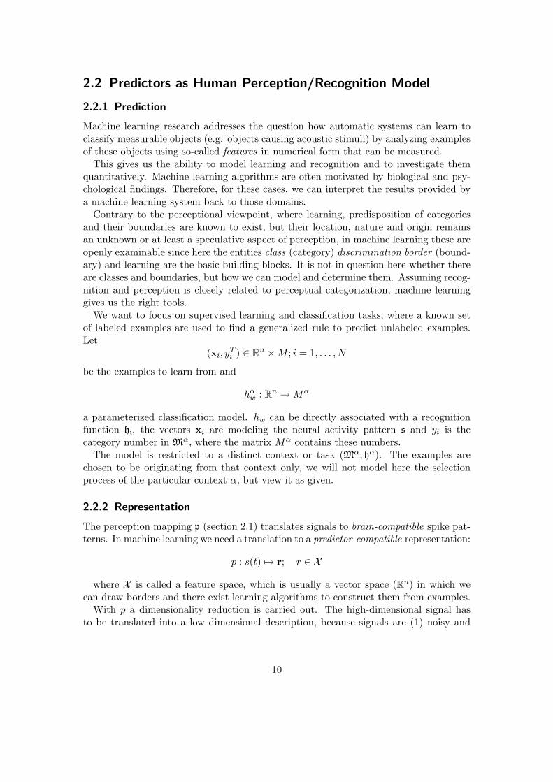
Calculating the time difference Time distance is a linear measure. In order to distin-guish sounds with a particular time structure from each other, we do not normalize time.For instance, we can distinguish running sounds from walking sounds by comparing thetime differences between consecutive foot steps. For these kinds of comparisons, we usetime values in seconds. However there are also cases, where relative temporal positionsof the onsets within a sound play an important role in the identification of the sound.Opening or closing door sounds can be typical examples for those cases. The time valuesfor those kinds of sounds are normalized.

However for both cases, the time difference is normalized so that the distance valuesare kept in the [0, 1] interval.

• For the normalized time case, a time value is normalized as follows:

tn = t−min(t)max(t)−min(t) .

Thus, the distance will simply be

dt(tn,1, tn,2) = |tn,1 − tn,2|.

• For the not normalized time case, the maximum time difference between the spikesof two sounds should be calculated. The maximum time difference can be betweenthe time between the very first spike of the one sound and the very last spike ofthe other sound.

tmax = max(abs(max(t1)−min(t2)), abs(max(t2)−min(t1)))

Hence, the distance will be

dt(tn,1, tn,2) = |tn,1−tn,2|tmax

.

These separate distances between amplitude, frequency and time values of the spikesare summed up to calculate the total distance between two spikes. After calculatingthe distance between two spikes, the distance between two spike-coded sounds can becalculated as explained in the following section.

A Distance Measure for the Spike-Coded Sounds

The distance between two spike-coded sounds is simply the normalized sum of the dis-tances between the corresponding spikes.

d(s1, s2) = 1N

∑Ni=1 d(s1

i , µ(s1i )),

where µ is a mapping between the spikes of the first sound and the second sound, whichis used for finding the corresponding spikes to calculate the distance. This mapping is afunction defined as

24

s2j = µ(s1

i ).

In order to find the mapping between the spikes of two given sounds a bipartite graphmatching algorithm is used.

In order to calculate the distance between two spike-coded sounds, the mapping be-tween the corresponding spikes of these two sounds should be defined. This mapping isdefined by using the Hungarian algorithm.

The Hungarian Algorithm

The Hungarian algorithm assigns the vertices of a weighted bipartite graph to each other,so that the maximum weight matching is achieved. In a maximum weight matching theweights must be non-negative.

Definition 1 A “weighted bipartite graph” is a graph G = (V = X ∪ Y, E = X × Y ),such that X ∩ Y = ∅, where an edge ex,y, x ∈ X, y ∈ Y has a weight w(ex,y).

In order to achieve minimum weight matching, the highest weight C should be found.Other weights should be subtracted from the maximum weight as follows: w(ex,y) =C − w(ex,y).

Suppose that two disjoint sets X and Y of the vertices have the same cardinality n.The weights are shown in an n × n matrix W . The total weights of the matching Mis to be maximized, w(M) =

∑e∈M w(e). A perfect matching is an M , in which every

vertex is adjacent to some edge in M . A maximum weighted matching is perfect.

Definition 2 A “feasible vertex labeling” in G is a real-valued function l on X ∪Y suchthat for all x ∈ X, y ∈ Y ,

l(x) + l(y) ≥ w(ee,y).

It is always possible to find a feasible vertex labeling. In order to initialize the algo-rithm with a feasible vertex labeling, we set all l(y) = 0 for y ∈ Y and for each x ∈ X,we take the maximum value in the corresponding row in the weight matrix, as follows:

l(x) = maxy∈Y w(ex,y),l(y) = 0.

If l is a feasible labeling, Gl is the sub-graph of G, which contains only those edges,where l(x) + l(y) = w(ex,y). This graph Gl is called the ”equality graph” of G for l. Aperfect matching M in an equality graph Gl has the following property

w(M) =∑

e∈M w(e) =∑

v∈V l(v).

25

The main purpose of the Hungarian algorithm is to find the maximum weight match-ing M in an equality graph Gl, by augmenting the matching M after each step. Ifaugmenting the matching M is not possible, by improving the labeling l to l′ a newequality graph Gl′ can be constructed, which enables to augment the matching M .

In order to improve the labeling, we need to define the neighbors of a single vertex uand a set S of vertices in Gl as follows:

Nl(u) = {v : (u, v) ∈ Gl},Nl(S) = ∪u∈SNl(u).

For a set S ⊆ X of the free vertices u and T = Nl(S) ⊂ Y . Set

δl = minx∈S,y/∈T {l(x) + l(y)− w(ex,y)}.

and

l′(v) =

l(v)− δl v ∈ Sl(v) + δl v ∈ Tl(v) otherwise

The consequences of the relabeling step are

• If (x, y) ∈ Gl for x ∈ S and y ∈ T , then (x, y) ∈ Gl′ .

• If (x, y) /∈ Gl for x /∈ S and y /∈ T , then (x, y) /∈ Gl′ .

• There will be some edge ex,y ∈ Gl′ for for x ∈ S and y /∈ T .

Theorem 1 (Kuhn-Munkres) If l is a feasible vertex labeling and M is a perfectmatching for Gl, then M is a maximum weight matching for G.

The Kuhn-Munkres theorem transforms the problem from an optimization probleminto a problem of finding a feasible vertex labeling whose equality graph contains aperfect matching of X to Y .

The Hungarian Algorithm:

1. Start with a feasible vertex labeling l, determine Gl, and choose a matching M inGl.

2. if M is a perfect matching, then M is maximum weight matching. Stop. Otherwise,there is some unmatched x ∈ X. Set S = {x} and T = ∅.

3. If NGl(S) = T find δl = minx∈S,y/∈T {l(x) + l(y)− w(ex,y)}.

26

4. Construct a new labeling l′ by

l′(v) =

l(v)− δl v ∈ Sl(v) + δl v ∈ Tl(v) otherwise

5. Note that δl > 0. Replace l by l′ and Gl by Gl′ .

6. If NGl(S) 6= T , choose a vertex y ∈ NGl

(S) and y /∈ T .

a) If y is matched in M , say with z ∈ X, replace S = S ∪ {z} and T = T ∪ {y}.Go to Step 3.

b) If y is free, and there will be an alternating path between the free vertices xand y. Construct this path M ′, and replace M by M ′. Go to Step 2.

The Hungarian algorithm provides the complete matching between the spikes of twospike coded sounds. By using this matching µ and the spike distance function (SeeSection 3.1.1), we can calculate the distance between two given sounds. Being able tocalculate the distance between two spike-coded sounds, enables us in turn to generatea distance matrix using these distances. Furthermore, one can define a kernel functiondeparting from the distance measure. In that case, the kernel function can be used in akernel machine to perform a classification task. In the following, it is explained in detail,how the spike kernel is defined.

The Spike Kernel

By using a kernel function, a non-linear classification problem can be transformed intoa linear classification problem in a higher dimensional feature space. In order to do this,a transformation function φ(x) should be defined, which transforms an input vector intoa feature vector in a higher dimensional feature space. The kernel matrix is defined as

k(x,y) = 〈ϕ(x), ϕ(y)〉.

Hence, in order to exploit the kernel substitution, a valid kernel function should bedefined. A valid kernel function is a function, whose Gram matrix is positive semi-definite.

One approach is to define the transformation function, and by using this function tofind the corresponding kernel. Generally, however we don’t need to define the trans-formation function explicitly to construct a valid kernel. One usual way to constructnew kernels is to make use of simpler kernel functions as building blocks to define morecomplicated kernels by simply combining the simple kernel functions in certain ways likeaddition or multiplication etc. In order to define the spike kernel, we use this combina-torial way.

The linear kernel is defined as

k(x,y) = 〈x,y〉.

27

The squared distance can be defined by using the linear kernel as follows:

||x− y||2 = k(x,x) + k(y,y)− 2 · k(x,y).

Since the spike distance is a weighted sum of the squared distances of each of the threeattributes of two spikes, we can define the spike distance by using the linear kernel inthe same way. The distance between the frequency attributes is calculated as follows:

κ(f1, f2) = k(f1, f1) + k(f2, f2)− 2 · k(f1, f2).

In the same way, we can define the distance between the amplitude and time attributesby using the linear kernel as well. In order to complete the spike kernel function, weneed to combine these three kernel functions in a weighted sum as follows:

d(s1, s2) = cf · κ(f1, f2) + ca · κ(a1, a2) + ct · κ(t1, t2). (3.1)

So, this kernel function defines the linear spike kernel. Even-though we use the spikedistance function in this kernel function, it is still linear in nature. However, we wantto define a kernel function, in order to solve non-linear classification problems. Beforedefining the non-linear spike kernel, we show the Gaussian kernel:

k(x,y) = exp(‖x−y‖2

2σ2 )

It is easy to see that the nominator of the exponential function is nothing but thesquared distance of the vectors x and y. We can simply replace the squared distancewith the linear spike kernel, defined in Equation 3.1 as follows:

κ(x,y) = exp(d(s1,s2)2σ2 )

The non-linear spike kernel function is incorporated in the support vector machinesto perform classification experiments.

3.1.2 Gammatone Filters based Representation

A gammatone auditory filter bank converts a given signal into a multi-channel basilarmembrane motion. Recent research has shown that a gammatone filter can approxi-mate the magnitude characteristics of the human auditory filter properly [11]. Hence agammatone filter bank simulates the spectral analysis step of the auditory processingof a given sounds performed by the basilar membrane very well. In the following, weintroduce two approaches to extend the basilar membrane motion biologically.

The first approach calculates the temporal envelope of each filter output by applyingthe Hilbert transform. The temporal envelope calculation is an essential part of theroughness estimation proposed by Zwicker and Fastl [53].

28

The second approach is the inner hair cell simulation by Meddis [31] [32]. The innerhair cells are connected to the basilar membrane. The inner hair cells convert themechanical transduction performed by the basilar membrane into a neural transductionby simply modeling the transmission rates of each cell into the cleft. A combination ofthe inner hair model with the gammatone auditory filter bank generates the auditoryimage of a processed sound.

Figure 3.2: Steps of preprocessing. The left side shows the representation that empha-sizes the spectral features of the signal. The right one shows the steps usingthe time domain analysis with the inner hair cell model. In the SVM exper-iments the whole sound example was used as signal s(t) in opposite to theHMM, for which the signal was windowed and the procedures were appliedon each frame resulting in a series of vectors vt

i .

After performing these two steps, namely applying the gammatone filter bank fol-lowed either by the Hilbert transform or by the inner hair cell model, a two-dimensional

29

representation is obtained. In the last step, this representation is integrated efficientlyinto a feature vector.

Figure 3.2 describes the 2 paths of preprocessing the input signal. Common is thebeginning with a gammatone filter bank and the last step to compress a sequence ofvalues into 4 values by using the Mean-Variance feature integration scheme.

Spectral content

Gamma-tone Auditory Filter-bank A gamma-tone auditory filter-bank [38] is the firststep of the cochlea simulation, where the basilar membrane motion is simulated in afilter bank. The impulse response of a gamma-tone filter is highly similar to the magni-tude characteristics of a human auditory filter, which makes the gamma-tone auditoryfilter bank a biologically plausible representation. With increasing center frequency, thespacing and the bandwidth of the gamma-tone filters increase, however the overlappingof each consecutive filter stays the same (equivalent rectangular bandwidth or shortlyERB [15]). ERBs are similar to the Bark or the Mel scale.

As a pre-processing of the everyday sounds, we use the gamma-tone filter implementa-tion in Malcolm Slaney’s Auditory Toolbox [44]. We use 18 gamma-tone filters in total.Therefore, for each given sound, we obtain 18 filter responses from the gamma-tone filterbank. The lowest center frequency used for the gamma-tone filter bank is flow = 3 Hz.It lies outside the audible frequency range captured by the Basilar membrane. But itcaptures, in addition, also features that refer to frequencies in the range of roughness or’rhythmical’ content. The highest center frequency used in the gamma-tone filter bankis fhigh = 17059 Hz roughly corresponding to the highest audible frequency.

The Gamma-tone filters can be combined with other representations, in order to obtaina more complete representation scheme.

Hilbert Transform The first method with which we combine the gamma-tone filters isthe Hilbert Transform [30]. The Hilbert transform of a signal is the convolution of thetime domain signal with 1

πt . Combining the Hilbert transformed signal with the originalsignal, we obtain the analytic signal. This process deletes the negative components ofthe signal in the frequency domain, and doubles the amplitudes on the positive side.Furthermore the analytic signal is a base band signal. The power spectrum of theanalytic signal is the modulation spectrum of the temporal envelope. In many roughnessestimations, this step is the very first step of the roughness estimation procedure [53].

Grouping in 4 bands However, the huge dimensionality of the power spectrum of eachfilter output should be reduced, in order to be able to create a feature vector for a sound.Therefore we summarize these values in four frequency bands [6] [7] by simply taking theaverage of the power values corresponding to these frequency bands. These frequencybands are the DC values, the frequency interval 3-15 Hz (syllable rate in speech, orrhythms), 20-150 Hz (roughness), and 150-1000Hz (low pass).

30

Temporal content

Inner Hair Cell Model To analyze the signal in time, we directed the output of thegamma-tone filters into the inner hair cell model of Meddis [31]. In this model, thefiring rate of the inner hair cells, connected to the basilar membrane, is modeled. Theinner hair cells fire, when a stimulus arrives. This happens when the basilar membraneis deflected at the point of a resonance frequency, where the hair cell sits. This firing issimulated by the dynamics of production and flow of transmitter substance. A certainamount of transmitter substance is released into the synaptic cleft between the haircell and another neuron, depending on the strength of the stimulus. For each arrivingstimulus, the Meddis inner hair cell model calculates these amounts iteratively. In ourrepresentation, we use the rate of transmitted part of the transmitter substance [47].

Feature Integration

In both analyses (3.1.2 and 3.1.2) we end up with a number of sequences of values thathave to be compressed into one final feature vector. We applied a feature integrationscheme that calculates the mean and variance of the sequence as well as the mean andvariance of the first derivative (difference of two consecutive values).

In the spectral content case these are 4 sequences (4 bands) of 18 energy values ofthe filters, which are compressed each to the 4 values described above. This makes afeatures vector of 16 values. Note, that the derivatives (deltas) were taken over the thefilter outputs, i.e. in frequency domain.

In the temporal case we used the same schema in the time domain. Here we had18 time sequences from the Inner Hair Cell model, which were compressed each to 4mean/variance values resulting in a 72 dimensional vector.

3.1.3 Other Representation Schemes

In the sequel, we will use other representations of sounds as a comparison.Mel Frequency Cepstrum Coefficients (MFCC’s) [27] are a well established represen-

tation scheme which dominates applications in speech recognition and music processing.It is based on a frequency spacing (Mel scale) inspired by the basilar membrane. Thisrepresentation allows to separate a signal into source (fundamental frequency) and filter(spectral shape) component. We use 13 MFCC coefficients, their variances, finite dif-ferences between consecutive MFCC coefficients and the variances of these differences,adding up to a 52-dimensional vector. MFCCs have rarely been applied to environmentalsounds. We will use them in Section 3.2.2.

As a comparison, we will use a feature set we will call Low-level spectral features (SLL).It consists of a 68-dimensional vector: the 13 MFCCs and four additional descriptors(signal energy, centroid, roll-off, zero crossings) their variances, finite differences and thevariances of the differences. They will also be used in Section 3.2.2.

A large set of features have been implemented in the Ircam descriptor by G. Peeters[39]. In Section 3.2.2, we will also use a feature set of timbre descriptors. It is a 19-dimensional feature that consists of mean and variance for spectral sharpness and spread,

31

and 12 dimensional signal auto correlation, roughness, energy modulation frequency, andenergy modulation amplitude. Sharpness is the perceptual equivalent to the spectralcentroid. Spectral spread measures the distance between the largest to the total loudnessvalue. Roughness, how it is used here, is based on the ERB scale.

The synthesized impact sounds in Section 4.4 will be represented by the following fea-tures. We will use unnormed timbre features (42 dimensions) consisting of: 6 dimensionsperceptual spectral centroid mean, 6 dimensions perceptual spectral spread mean, meanenergy, energy modulation frequency, effective duration, temporal decrease, temporalcentroid, loudness mean, relative specific loudness mean.

In Section 4.4, we will represent car horn sounds by the three dimensions: fundamentalfrequency, roughness, and spectral spread.

3.2 Evaluation

3.2.1 Spike Representation

In order to show that this new approach works generally well for simple everyday sounds,we performed two experiments on two simple data sets. The first data set containsfootstep sounds of running vs. walking people on different floor types. In order thatthe sounds are homogeneous, we prepared sounds of 10 footsteps each. Figure 3.3 showsone running and one walking sounds. Both of these sounds are spike coded, wheretime component is not normalized, simply because running and walking can easily bedistinguished by comparing the time between consecutive footsteps.

Figure 3.3: One spike coded running and one spike coded walking sound are shown incomparison.

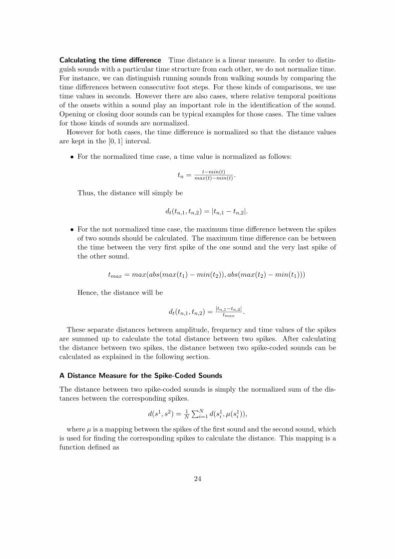
The second data set contains single footstep sounds on two different floor types, namelyon leaves and on marble. In this experiment, we normalized the time component in thespike coding. Figure 3.4 shows two spike coded sound examples, one footstep one marbleand one footstep on leaves.

32

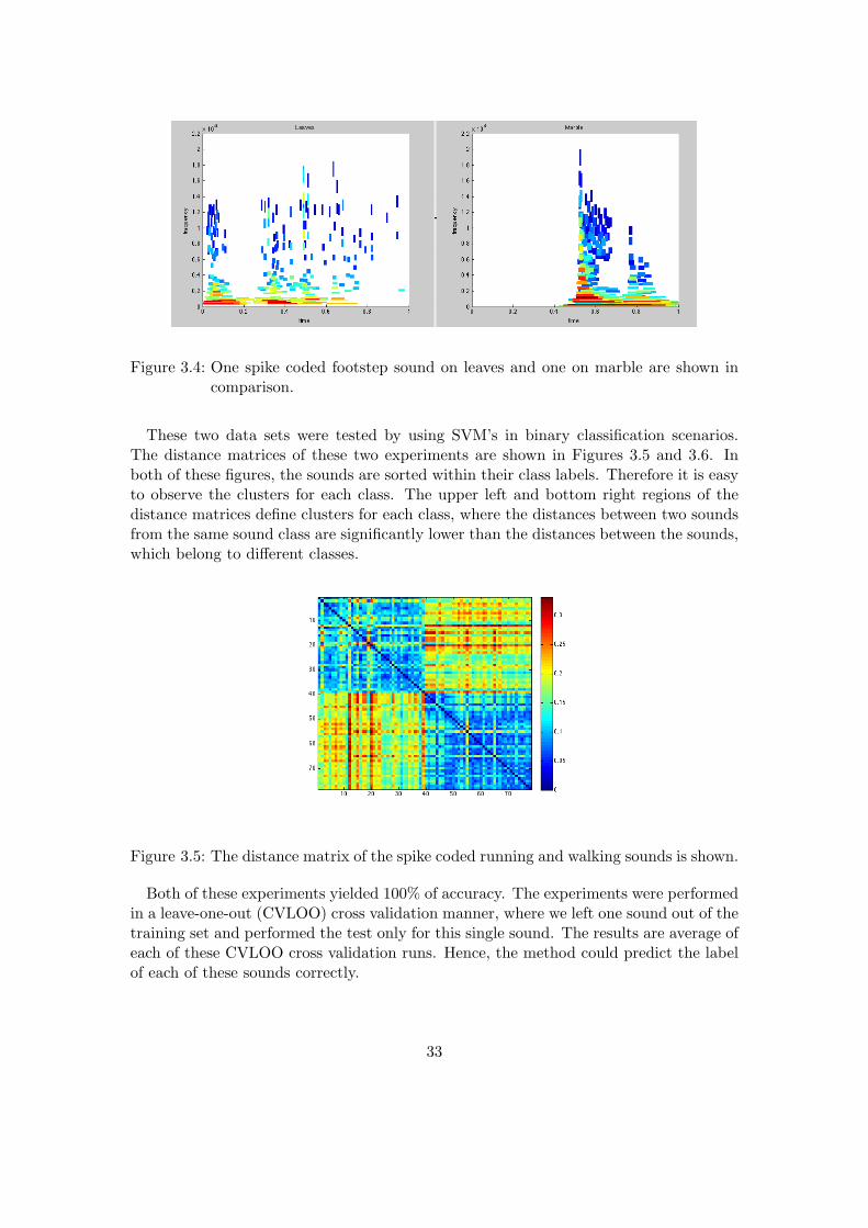
Figure 3.4: One spike coded footstep sound on leaves and one on marble are shown incomparison.

These two data sets were tested by using SVM’s in binary classification scenarios.The distance matrices of these two experiments are shown in Figures 3.5 and 3.6. Inboth of these figures, the sounds are sorted within their class labels. Therefore it is easyto observe the clusters for each class. The upper left and bottom right regions of thedistance matrices define clusters for each class, where the distances between two soundsfrom the same sound class are significantly lower than the distances between the sounds,which belong to different classes.

Figure 3.5: The distance matrix of the spike coded running and walking sounds is shown.

Both of these experiments yielded 100% of accuracy. The experiments were performedin a leave-one-out (CVLOO) cross validation manner, where we left one sound out of thetraining set and performed the test only for this single sound. The results are average ofeach of these CVLOO cross validation runs. Hence, the method could predict the labelof each of these sounds correctly.

33

Figure 3.6: The distance matrix of the spike coded footsteps on leaves and on marble isshown.

3.2.2 Representation Comparison

For the experiments, recordings of footsteps and doors are selected from the soundcollection “Sound Ideas” [22].

The footsteps are a subset of the Foley collection. It consists of recordings of differentkinds of shoes (heels, boots, barefoot, sneakers, leather) on various grounds (concrete,wood, dirt, metal, snow, sand). We picked the following movement modes: walking,running, jogging from male and female subjects. The recordings are cut, when neces-sary, such that exactly one step is contained in one sample. For the experiments onconcrete and wood floor (Tables 3.2, 3.3) we used 44 files per class and in the last 6-classexperiment we used 40 files per class (Table 3.4).

We performed experiments on different sole types, namely barefoot, sneakers, leather,heels and boots. These sole types were classified on two different floor types, namelyon concrete and wood floor. Furthermore, we performed an experiment to classify sixfloor types ignoring the sole types. These floor types were snow, sand, metal, dirt, wood,concrete.

The labels of these data-sets are mostly psycho-acoustically validated. We did notperform detailed psycho-acoustical experiments, but we checked the sounds by listen-ing to them by ourselves. We discarded sounds whose class cannot be identified whilelistening to them.

In order to evaluate the results of our experiments with the gammatone based repre-sentation schemes, MFCC, low level and timbre descriptors (cf. Section 3.1.3), we usedleave-one-out cross validation, where all sounds but one are incorporated into the train-ing set. Then the trained algorithms are tested on the remaining single sample thatpreviously had been excluded from the training set. This procedure is repeated for allpossible partitions into training/test sets.

The results of the experiments opening vs. closing door sounds are shown in Table 3.1.

34

The table shows the results of SVM and HMM classifications using two different rep-resentations: 1) gamma-tone filters combined with the Hilbert transform (GT Hil), 2)gamma-tone filters combined with the inner hair cell model (GT Med).

SVM HMMGT Hil GT Med GT Hil GT Med84.0% 63.2% 57.2% 70.0%

Table 3.1: Classification of opening vs. closing door sounds

We performed multi-class experiments for footstep sounds, where we used five differ-ent sole types on concrete floor, performing five separate binary classification runs. Ineach run, one class is classified against the rest, which consisted of the other 4 classes.Therefore the rest-class constituted a heterogeneous mixture of sounds. We took theaverage of these five binary classifications. Table 3.2 shows not only the overall averageof the separate classification experiments, but also the results of the separate binaryclassification experiments.

The percentages are 100% - BER (balanced errors rate), thats weights the two classerrors equally. First we look at classification of shoe types on concrete.

SVM HMMMFCC SLL TD GT Hil GT Med GT Hil GT Med

Barefoot 94.4% 94.4% 98.6% 97.7% 99.7% 85.2% 94.0%Sneakers 76.6% 82.1% 76.1% 90.1% 83.0% 73.2% 74.6%Leather 100% 100% 91.8% 90.1% 92.6% 90.0% 92.0%Heels 100% 100% 98.8% 95.9% 97.1% 88.0% 89.4%Boots 70.0% 72.5% 86.1% 94.3% 92.1% 89.9% 84.6%

Average 88.2% 89.8% 90.3% 93.6% 92.9% 85.3% 86.9%

Table 3.2: Experiment 1: Classification of the sole types on concrete floor

The same sole types hitting a wooden floor were classified in experiment 2. Follow-ing the same criteria as explained before. The results for this experiment are shown inTable 3.3. Note that the Sneakers class yielded the lowest accuracy, decreasing dramat-ically this result for gamma-tone Meddis based representation. A particular feature ofSneakers is their noisy characteristics compared to the other types of shoes.

In the third experiment (Table 3.4) we classified different floor types: snow, sand,metal, dirt, wood, concrete. The gamma-tone based representations outperformed theother methods. Dirt is not classified as well. This could be linked to its more complextemporal structure and its rather inhomogeneous sound character. Note that the timbredescriptors chosen are not suitable in this classification task. However, as future work,further exploration of new combinations of timbre descriptors [39] is needed.

Except in one case SVM performed better than HMM. For shoe type, on average thepower spectrum based method (left in Figure 3.2) performed better than the Meddisbased right method. However for the floor types the Meddis based method clearly

35

SVM HMMMFCC SLL TD GT Hil GT Med GT Hil GT Med

Barefoot 83.1% 95.9% 92.2% 95.6% 95.9% 88.0% 84.3%Sneakers 81.7% 83.7% 76.5% 87.5% 75.9% 69.8% 67.2%Leather 93% 97.7% 92.7% 98.5% 94.8% 91.6% 89.8%Heels 99.7% 99.7% 97.7% 98.5% 100% 98.8% 99.4%Boots 95.9% 96.5% 90.1% 96.2% 92.7% 88.1% 92.7%

Average 90.7% 94.7% 89.8% 95.3% 91.9% 87.3% 86.7%

Table 3.3: Experiment 2: Classification of the sole types on wood floor

SVM HMMMFCC SLL TD GT Hil GT Med GT Hil GT Med

Snow 96.5% 98.7% 93.3% 90.0% 99.5% 94.0% 89.9%Sand 90.8% 98.5% 86.3% 86.4% 91.0% 88.2% 92.8%Metal 97.5% 98.5% 85.8% 86.2% 98.8% 89.2% 92.9%Dirt 61.7% 82.5% 72.8% 77.7% 90.0% 77.5% 83.1%

Wood 96.0% 98.8% 87.8% 98.3% 100.0% 89.4% 94.8%Concrete 88.7% 88.9% 82.5% 91.5% 98.0% 92.5% 89.3%Average 88.5% 94.3% 84.7% 88.4% 96.2% 88.5% 90.5%

Table 3.4: Experiment 3: Classification accuracy of the floor types

performs better.

3.2.3 Outlook: General Everyday-Sounds Classification

In order to generalize the prediction performances of the representation schemes weprovide, we need to define a general sound database corpus according to the resultsobtained by the soundscape and categorization studies on everyday sounds.

Vanderveer’s categorisation experiments [49] revealed that human beings groupedsounds together either because they were similar or because they were produced bysimilar events. Different levels of abstraction are used, when grouping sounds into asound category. These abstraction levels are used in defining the categories or even acomplete taxonomy as well. Gaver [14] proposed a hierarchical taxonomy of sound eventsdepending on the information about an interaction of materials at a location in an en-vironment. He claims that a sound event occurs due to the interaction of two materials.Therefore, Gaver proposed a general level in this hierarchy depending on the generalcategorisation of these materials, namely solid, liquid and gas. Univerona made use ofthe taxonomy to develop their physically-based sound models, and in turn extended thetaxonomy depending on the sound-producing events. Even-though the taxonomy devel-oped by Univerona depends basically on Gaver’s taxonomy, there are differences betweenthem depending on the low-level models developed by Univerona used for creating basicsound events.

36

Gaver defined the sub-categories within the solid sounds as deformation, impact, scrap-ing and rolling sounds. Univerona defines fracture, impact and friction as the low-levelmodels generating vibrating solid sounds. Among the two categorisation schemes, onlythe impact sounds are common. Scraping and friction can also be considered as similar.Univerona defined rolling sounds as a compound category consisting of infinitely manyimpact sounds. Hence impact model generates also the rolling sounds. In the Univeronataxonomy, deformations like crushing and breaking are defined as compound categoriesconsisting of fracturing and impact sounds. Vacuum cleaners, balloons, steam and windsounds are categorised in the wind sounds.

In Gaver’s taxonomy, liquid sounds are categorised as drip, pour, splash and ripple,whereas Univerona has only two sub-categories, namely bubble and flow. In Univerona’staxonomy, dripping is a combination of bubble sounds with impact sounds from the solidsounds category. Pouring is even one level higher in the hierarchy. Univerona definespouring as a combiantion of dripping and flowing. Splashing is a complex form of drip-ping. Hence, splashing is one level higher in the hierarchy as well. Gaver divides the gassounds into three sub-categories: explosion, whoosh and wind. Univerona, on the otherhand, has only two categories. These two categories are turbulance and explosion. So,explosion category is common in these two models. In Univerona’s taxonomy, turbulancemodel generates whooshing sounds.

The Gaver taxonomy is an ecological approach depending on the assumption thatsounds provide information about the interaction of the materials. The taxonomy pro-posed by Univerona is formed based on the Gaver taxonomy depending on the low-levelsound models, generating everyday sounds. In this respect, the Univerona taxonomycan be considered as a realisation of the taxonomy proposed by Gaver. There are othertaxonomy schemes categorising everyday sounds into basic and compound sound classesconsidering the perceptual issues as well.

We generate our general everyday sounds database, considering these two taxonomyschemes in combination. We selected the sounds from the Sound Ideas database. Thesemantic descriptors of the Sound Ideas database are used for labelling the sounds. Weused a hierarchical categorisation as well. In the lowest level of this hierarchy, we dividedour sound database into three main sound categories, namely solid, liquid and gas.

The solid sounds category consists of four sub-categories. These are impact, rolling,deformation and friction sounds. Impact sounds are selected to be switches, singletypewriter clicks and hitting sounds. The rolling sounds are selected to be the car enginesounds in the idle state. Gaver indicates the regularity in the rolling sounds. Car enginesin their idle state make regular rolling sounds. Therefore these sounds can represent therolling sound category properly. We simply cut 4 sec. long snippets of the car enginesounds. Car crashes and glass crashes sounds constitute the deformation sounds. Thefriction sounds category consists of squeaking and sliding doors, windows and draggingsounds. The liquid sounds are sub-divided as pouring, dripping and flowing sounds.Pouring sounds category consists only of pouring sounds. However the dripping soundscategory constitutes dripping, splashing sounds as well as rain and waterfalls. Simpledripping sounds are quite different than rain or waterfall sounds, but in the taxonomieswe refer to, they are considered as dripping sounds as well. In the Univerona taxonomy,

37

pouring sounds are considered as a combination of dripping and flowing, but we stick tothe Gaver taxonomy in this case, and distinguish pouring sounds from dripping sounds.Filling, waves coming in and running (flowing) water sounds are grouped in the flowingsounds category. Considering the fact that pouring sounds generally fill a bottle or acan with running liquids, pouring and flowing sounds can be grouped together as well,which is the case in the taxonomy of Univerona. The sub-categories in the categoryof gas sounds are explosions, wind and whooshing sounds. Explosions and gunshotssounds are considered as explosions. Passing airplanes or cars, flame thrower sounds,fire burst sounds, arrows and knifes are grouped in the whooshing sounds category. Thewind sounds category consists of wind, vacuum cleaner sounds, air, balloon and steamsounds. The vacuum cleaner sounds generate not only wind sounds but also rollingengine sounds. So, they can be considered in both of these categories.

This sound database corpus will be classified by using our representation methods.These classification experiments will provide us the generalizability of our representationmethods onto each of these everyday sound categories. Furthermore, the classificationresults will be analyzed further, in order to extract the perceptually relevant features,which play an important role in the classification.

38

4 Case study: Impact Sounds

The aim of this case study is to achieve Milestone M1: Analysis, classification and mea-surement of functional sounds. It is based on findings from WP4 (context information)and WP2 (physical modeling parameters).

The collision of solid objects generates sound that is a basic building block for manyeveryday sounds. Either as a single event or as a composition. The information conveyedby the sound of colliding solids is manifold: weight, material, used force, shape andothers (see and considerations and literature review in D4.1 [19] section 1.1.2). In thiscase study we focused on the perception of the material of hammer struck solids.

This chapter is organized in two separate studies: 1. Learning how to control animpact sound generating process using perceptual information from subjects. 2. Usingthe spike representation for impact sounds for automatic classification to perceptualcategories.

Both studies use the data acquired by our partners at IRCAM (WP4) using a physicalsound model by UNIVERONA (WP2).

4.1 Perceptual control of Impact Sound Synthesis

Developing tools for sound design requires a notion about the perceptive function ofsynthesized sound. This is provided by the designer. For the design process it is impor-tant to take into account what information a subject (a user of product) perceives whenhearing a functional sound.

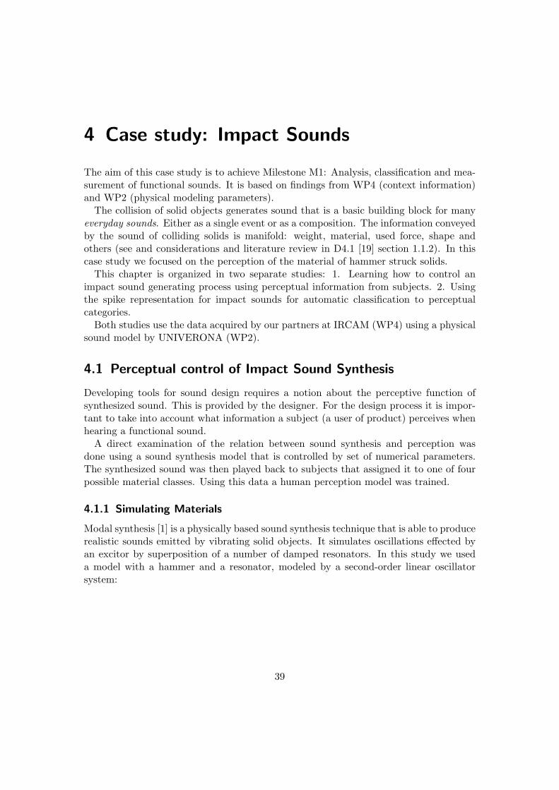
A direct examination of the relation between sound synthesis and perception wasdone using a sound synthesis model that is controlled by set of numerical parameters.The synthesized sound was then played back to subjects that assigned it to one of fourpossible material classes. Using this data a human perception model was trained.

4.1.1 Simulating Materials

Modal synthesis [1] is a physically based sound synthesis technique that is able to producerealistic sounds emitted by vibrating solid objects. It simulates oscillations effected byan excitor by superposition of a number of damped resonators. In this study we useda model with a hammer and a resonator, modeled by a second-order linear oscillatorsystem:

39

x(h)i + g

(h)i x

(h)i +

[ω

(h)i

]2x

(h)i =

1

m(h)il

(f (h)e + f) , i = 1 . . . N (h)

x(r)j + g

(r)j x

(r)j +

[ω

(r)j

]2x

(r)j =

1

m(r)jm

(f (r)e + f) , j = 1 . . . N (r)

x =N(r)∑j=1

t(r)mjx

(r)j −

N(h)∑i=1

t(h)li x

(h)i

v =N(r)∑j=1

t(r)mj x

(r)j −

N(h)∑i=1

t(h)li x

(h)i

f(x, v) =

{kx(t)β + λx(t)β · v(t) if x > 00 if x ≤ 0

(impact force),

where x is the oscillator displacement, f an external driving force. Index (h) denotesthe excitor (hammer) and (r) the resonator (hit object). The two oscillator systems areparameterized each by g the damping coefficient, ω the oscillator center frequency andmij the mass of the object at a given point (i, j). For any point (l,m) the resultingdisplacement x is calculated using the matrix T that decouples the oscillator equations[1]. The last equation describes the driving force f(x, v) that couples the hammer andresonator. For more details on this see also [21] and [40].

Modal synthesis is specialized on solid compact objects rather than modeling vibratingair in tubes or strings of instruments. Because we are interested in everyday sounds itis the right tool to study them as long as we are dealing with solids like shoes, wheels,doors or other mechanical devices. A large fraction of everyday sounds is covered.

Hitting solid objects emits sounds that convey information about the material of boththe excitor and the resonator. We confine ourselves to look at the material of theresonator only, while keeping the excitor fixed for the sake of simplicity.

Referring to the equations of the modal synthesis above, one can count for each mode3 parameters (gi, ωi,mil) for hammer and resonator plus the 3 coupling parameters k, λand β. Given a 2-modal system used for resonator and a fixed setting for the hammerthere are 9 parameters to adjust. Tests show this is enough to simulate cartoonifiedimpact sounds of the resonator materials glass, metal, plastic and wood.

The system is a transformation of a parameter vector θ = (g1, g2, ω1, ω2,m1,m2, k, λ, β)T

to a a signal s(t), which is listened and categorized by a subject according to the per-ceived material

m ∈ {Cglass,Cmetal,Cplastic,Cwood},

where Cx is the label number of the material class x (see top part of figure 4.1).The key question we want to address here is: How can we produce material sounds

efficiently to meet the perceptive expectation of a certain material?

40

4.1.2 Prediction of Material Classes

The link between material perception and synthesis parameter settings and the signalis still missing. In particular we are looking for the mapping h : θ 7→ m predicting thematerial from the input parameters (see also figure 4.1). h can be applied as a sounddesign tool to give feedback to the designer.

Figure 4.1: models of perception

To solve the task of predicting materials we use methods of machine learning usingexamples, that can be obtained from psychoacoustic experiments (section 4.1.3). First,let

m ∈ {−1, 1}

be a binary classification task. We seek a classification function:

h(xi) = sign(〈ϕ(xi),w〉+ b) = yi

ϕ(xi) being a feature vector (= ϕ(θ)) and yi the prediction of m given xi. Eitherside of the discrimination border 〈ϕ(xi),w〉+ b belongs to one of the two classes. K isalways a linear or non-linear Kernel function (compare section 2.2.3) with 〈ϕ(x), ϕ(x′)〉 =K(x,x′). Finding w and b such that the model will predict correctly the example datawhile generalizing (minimize the generalization error) is the task to solve.

The advantage to use the modal synthesis rather than recordings is, that we are ableto produce a wide spectrum by sampling the parameter space to cover it equally undersimilar conditions and thus can infer a general rule for solid sounds.

The parameters of the modal synthesis can be used directly as features of the impactsound. These features are generative, since they are not calculated from the signal, butare used to generate it. Still, they are sound descriptors that, given the synthesis process,determine the sound and the material.

We have to deal with the fact, that not all possible parameter vectors generate nec-essarily a material sound, not even an audible sound. To generate feasible examplesto train a prediction model it is necessary to filter out those non-material sounds. Ina dynamic system that can show chaotic behavior there is no direct way to do this byanalyzing the parameters. Thus, in the first stage of the psycho-acoustic experiments amanually selected set of parameters vectors was used, which were validated by a humanto be a good sound. The size of this manually selected set is limited though, in thesecond stage we plan to use a larger one that needs to be generated automatically.

41

Subject

x

y

Synthesizer

model

query

data pool

soundx

Figure 4.2: Setup of a psychoacoustic experiment using Active Learning

4.1.3 Experiments

The experimental setup is shown in figure 4.2. We used active learning (section 2.2.4) tooptimize the learning progress. The synthesis model used is governed by 9 parameters(section 4.1.1). We chose 6 of them that influence the generated sound significantly.These are the parameters of the 2 resonators. The 6 parameters span the input space.We are looking for the 4 regions in that space that belong to the materials.

The approach of quantisizing the input space and let these examples be labeled bysubjects fails for 2 reasons: (1) The 6 dimensions cannot be densely sampled1 and (2)the mapping Θ M is only partially defined: not all parameter combinations inducea clear material sound. Either the sound is too synthetic or not audible. Therefore, asmall set of sounds was chosen manually [28] by experimenting with the sound model.This yields a complete surjective mapping Θ′ → M, where Θ′ = {θ1, θ2, . . . , θn} is adiscrete set of parameter vectors 2.

The experiments were done using the two sets: Θ′ and Θ′red ⊂ Θ′ with a size of 372

and 196 examples respectively, since the subjects labeled the same sounds differently. Asmall analysis revealed that none of these sounds have been labeled by the subjects thesame. These differences caused inconsistencies within the data set. In order to get rid ofthese inconsistencies, IRCAM generated a sub-set of the same data set from consistentlylabeled sounds. The reduced set is a more restricted selection in terms of consistencybetween the subjects. The examples with the most disagreement were removed andconsidered to be ambiguous.

In the complete data set experiments, we did binary and four-class classification ex-periments with 372 impact sounds. These four classes are the material classes, namelywood, plastic, glass and metal. In the binary experiments, wood and plastic as well asglass and metal classes are summarized in one class. These sounds have been labeledby 20 subjects in psycho-acoustics experiments, performed by IRCAM. We simulated

110 steps per dimension would 1 million sample points2Instead of manually selecting examples it is planned to use an automatic selection process that yield

a much larger set Θ′′ to choose from. To get good examples we would need again a predictor thatcan distinguish between material and non-material sound, see section 4.1.5.

42

each subject separately. Therefore we obtained 20 different classification results. Eachof these results can be considered as the simulation of one particular subject.

Generally the accuracy of the results are satisfactory. However, for some subjects,namely 6, 7, 8, 10, the binary classification results are worse than the four class classi-fication. Note, that not all available label information was used, but the training wasstopped after 30 labels. This was done to simulate that in a psychophysical experimentsthe number usable labels will always limited.

4.1.4 Results

Figure 4.3 summarizes the the results of the predictors trained with active learning asboxplots (see figures 4.6 and 4.7 for detailed results). The training algorithm used 20labeled examples and 252 unlabeled examples. The rest of 100 examples were used fortesting, from which the resulting prediction error were calculated for each subject.

The 4 class experiment shows a much higher error rate than the 2 class experiment.This is due to 2 reasons: A guessing predictor in a 4-class task would converge to a rateof 75%, while a binary one would go to 50%. Secondly, the task is in general harder forfour classes, since there the 4 class predictor, that is constructed of 4 binary ones, has tofind a model that suites all classes evenly well. Still, even the 4 class prediction here isclearly better than guessing and the binary task is fairly good, taken into account thatis has only seen 20 examples. The reduction of label noise in the reduced data set helpstraining as expected in both prediction tasks.

4.1.5 Discussion

For the data given, the results are very promising. Nevertheless for practical applicationwe need a significant improvement. This can be achieved by using a much larger poolof unlabeled data. Acquiring more data points that can be used for training is possible:

1. Having a method to decide whether a sound is a material sound or not would giveus a possibility to sort out those points that are not of interest. Psychoacousticmeasures for loudness and can help here.

2. Introduction of a 5th negative class: When a sound is played the subject candecide to label it undecided or not audible. This way one could use the physicalmodel directly in the experiment. The crucial point here is how much is the ratioof non-material sounds to material sounds. If there are much more non-materialsounds – as it seems to be – the training set would have be very unbalanced andtraining would take longer than a subject can do it. Furthermore subjects aregoing to label sounds in-between two classes (metal/glass) as undecided and lowerthe amount of positive examples. Studies on forced-choice decision making willhave to be consulted.

43

4−class full 4−class reduced 2−class full 2−class reduced0

0.1

0.2

0.3

0.4

0.5

0.6

0.7

0.8

0.9

1ba

lanc

ed p

redi

ctio

n er

ror

Figure 4.3: Prediction error after training with modal synthesis parameters. Each ex-periment simulation was carried out with 20 subjects. The test results areshown as boxplots of the 20 trained human prediction models. The centerred line is the median error rate, whereas the box covers 50 % of the resultdistribution. See detailed results at the end of this chapter.

4.2 Representation of Impact Sounds

The input parameters θ of the physically based sound model determine the sounds,which have been synthesized and saved as audio files (samples) in order to generate afeature-based representation of the signal. For these sounds we generated spike coderepresentations using a gammatone filter bank with 256 filters. The number of spikeswas fixed to 16 spikes per sound example. The representation method was presented insection 3.1.1. Since these impact sounds are relatively short, only 16 spikes are sufficientto code the perceptually relevant parts of these sounds.

In these experiments, similar to the experiments presented in Section 4.1.3, each sub-ject is modeled separately. We modeled four class experiments as well as binary classi-fication experiments. In these experiments, the complete data set and the reduced dataset are used.

4.2.1 Results

The results of the complete as well as the reduced data sets are shown in Figure 4.3.This figure indicates better results than the results obtained by using the physical modelparameters. The input parameters of the physical model are generative parameters tosynthesize these sounds. However generative parameters do not necessarily reflect the

44

Figure 4.4: The sound signal s(t) is represented by r, which is used to train the perceptionmodel.

perceptual features, which play an important role in the classification of these sounds.However the spike coding representation scheme is based on biological and psychophys-ical studies, where the perceptual behavior has been investigated thoroughly. Thereforethis representation scheme encodes the perceptually relevant features in classification ina better way than the physical model parameters. The results we obtained by theseexperiments also encourage us to claim that the spike coding combined with the Hun-garian algorithm is a proper way to encode given sounds from a classification point ofview.

The results are shown in figure 4.5. As expected the results obtained with the reduceddata set are far better than the results obtained with the complete data set.

4.3 Conclusion

From the results of these experiments with synthesized impact sounds we conclude:1. The division of the control parameter space into 4 regions was possible, but we

have to accept a considerable error. This shows that the selected generative featuresand the perception of materials is not straight forward. This has to be considered whenbuilding tools. Solely using control parameters with human labeling as measurement isnot sufficient.

2. The division of the feature space using a spike representation with a kernel thatmeasures similarity between spike patterns yielded good results. We could achieve pre-diction rates that are feasible to use. Here the the perceptual information about the ma-terial is available and the feature space is flexible enough to allow successful classificationdepending on the notion about materials of the subject, which can differ significantly.

4.4 Outlook: Preliminary Experiments with Timbre Descriptors

In order to further understand the nature of spike coding in a better way, and to studyits performance comparatively, a comparison with timbre descriptors will be fruitful.Moreover, the timbre descriptors can be compared with the descriptor built from thegamma-tone filter bank and subsequent inner hair cell model (GT Med), for the same

45

4−class full 4−class reduced 2−class full 2−class reduced0

0.1

0.2

0.3

0.4

0.5

0.6

0.7

0.8

0.9

1

bala

nced

pre

dict

ion

erro

r

Figure 4.5: Prediction error after training with spike coded impact sounds. Each ex-periment simulation was carried out with 20 subjects. The test results areshown as boxplots of the 20 trained human prediction models. The centerred line is the median error rate, whereas the box covers 50 % of the resultdistribution. See detailed results at the end of this chapter.

reason. These comparison experiments should be performed on the entire group ofsubjects separately. These results will enable us to gain insights of the psychoacousticalrelevance of the representation schemes properly.

4.4.1 Car Horn Sounds

In another preliminary experiment we compared 41 sounds. Subjects have been askedto judge whether the sounds are car horns or not [25]. According to the average answersof 31 subjects the sounds are grouped into car horn and non-car horn sounds. Withsupport vector machine, the leave-one-out procedure, and the grid search method weyield a balanced recognition rate of 73.56% when using the GT Med representation and84.93% when using a 3-dimensional representation consisting of fundamental frequency,roughness, and spectral centroid. However, a sound corpus of only 41 sounds cannotyield significant results about a high-dimensional representation scheme like the GTMed representation. In order to draw meaningful conclusions about these kinds of high-dimensional representation schemes, they should be evaluated by using larger data sets.Therefore we will redo these experiments using data sets consisting of sufficient numberof sounds.

46

0 2 4 6 8 10 12 14 16 18 200

0.1

0.2

0.3

0.4

0.5

0.6

0.7

0.8

0.9

1

subjects

bala

nced

err

or r

ate

full datasetreduced dataset

Figure 4.6: Results 4-class prediction with Active Learning using synthesis parameters

0 2 4 6 8 10 12 14 16 18 200

0.1

0.2

0.3

0.4

0.5

0.6

0.7

0.8

0.9

1

subjects

bala

nced

err

or r

ate

full datasetreduced dataset

Figure 4.7: Results 2-class prediction with Active Learning using synthesis parameters

47

0 2 4 6 8 10 12 14 16 18 200

0.1

0.2

0.3

0.4

0.5

0.6

0.7

0.8

0.9

1

subjects

bala

nced

pre

dict

ion

erro

r

full datasetreduced dataset

Figure 4.8: Results 4-class prediction with Active Learning using spike representation

0 2 4 6 8 10 12 14 16 18 200

0.1

0.2

0.3

0.4

0.5

0.6

0.7

0.8

0.9

1

subjects

bala

nced

pre

dict

ion

erro

r

full datasetreduced dataset

Figure 4.9: Results 2-class prediction with Active Learning using spike representation

48

5 Alternative Approaches

5.1 Adaptive Bottle Experiment

5.1.1 Introduction

Previous research on product-sound quality evaluation [4] shows that sound quality canbe described as the adequacy of a sound attached to the product. This measure is thecombinatory perception different qualities. As in the Bauhaus’ notion, that basic designelements are always linked to their dynamics and only perceived together (line is a causeof a moving point [23]), we follow this principle in product design looking at sound,object and interaction, which are examined by their combined aesthetics. We investigatethis by using prototypical design elements: The sounds generated are cartoonified, theobject is an abstract bottle like vessel and the interaction is exemplified by a tiltinggesture. There is a threefold interrelationship between these aspects: The bottle shapeof the object induces a gesture which causes sound that gives feedback and influencesthe gesture. The changing sound in turn causes a different perception of the object itself(bottle empty/full) that affects the gesture (figure 5.1).

Sound design as the synthetic generation of sound and aesthetic decision making bycontrolling the synthesis parameters can be combined with the product and its usage bypreference learning in a parameter mapping task [20]. In this respect, physically basedsound design offers a novel alternative to recording sounds [40]. We measure adequacyof the generated sounds through judgments of subjects interacting with the object, andoptimize the quality of the sounds using statistical methods iteratively.

Instead of an unguided trial and error process to find the best parameter settings interms of adequacy to the product function, we propose to substitute it by a guided one,depending on preference judgments. Here, we show an abstract implementation of thisidea: the Adaptive Bottle.

Adaptive Bottle is an interactive object, that has been designed to simulate the –suggested by the shape of the object – action of pouring [12]. It is connected to aphysically based sound model that simulates the sound of drops or small objects hittingthe surface of a resting liquid (dripping / splashing) [48]. The bubbles sounds supportthe interaction with the bottle. Therefore they are supposed to give the user the rightfeedback to measure how full it is.

The sound design task is to tune a physically based sound model to produce a desiredsound by adjusting it’s input parameters based on judgments.

49

Gesture

Sound�

���@

@@@

Shape

Figure 5.1: threefold aesthetics

5.1.2 Adaptive Bottle Optimization

The Adaptive Bottle has a built-in accelerometer, and communicates with the bubblessound model via the wireless interface of the chip. The acoustic model in [2], based onthe use of large quantities of bubbles to represent complex liquid sounds, has been im-plemented in the Max/MSP environment. It has seven input parameters, which controlthe statistics of bubbles size, intensity of emission, and rate of bubbles formation. Theseparameters are used for determining the characteristics of the sound. In this paper, thebubbles size and formation rate parameters are selected for the optimization. The otherparameters have been kept constant.

The accelerometer sends 3D orientation information to the computer. By using thisinformation, the tilting angle is calculated. Based on the tilting angle, the volume ofliquid remaining in the bottle is calculated. Remaining liquid is used in turn to deter-mine the current bubbles size and the current formation rate. By using the accelerationinformation, calculated formation rate and bubbles size, and the other synthesis pa-rameters, which are constant, the physically based sound model generates the bubblessounds. Figure 5.2 shows this information flow during the whole pouring action. At thebeginning of the interaction, it is assumed that the bottle is full. As the subject tiltsthe bottle, liquid is poured out, and the bottle becomes slowly empty, depending on thetilting angle. The amount of liquid in the bottle and the emerging bubbles sounds areupdated depending on the tilting angle. Intuitively speaking, the size of the bubblesemerging decreases, as the bottle gets empty during the action of pouring. The soundof larger bubbles in pitch is lower than of smaller bubbles. Therefore the bubbles sizedecreases, as the bottle gets empty.

Least Squares Optimization

The basic idea behind this optimization is to find the direction and the amount of theoptimization step to be made in that direction depending on the evaluation of four samplepoints, which is supposed to improve the quality of the produced sound. We minimize theunknown preference function by gradient descent. Thereto we model the near surroundof the sample point linearly. The direction of a learning step is the gradient of the linearleast squares solution. The mathematical formulation of this method according to theAdaptive Bottle problem is as follows:

1. The four data points xit around the central data point xt obtained in the last

iteration, which are to be evaluated by the subject are generated. Each of these

50

Figure 5.2: The interaction between the subject and the Adaptive Bottle is shown. Theacceleration parameters are used for calculating the new volume of the liquidremaining in the bottle, the formation rate and the size of the bubbles. Theformation rate and the size of the bubbles are combined with the otherparameters to generate the sounds.

four points are shifted to the origin, and each dimension is normalized separately.

xit = xt + rt ·

[cos π·i

2sin π·i

2

], i = 1, . . . , 4 (5.1)

A =

x1

tT

x2tT

x3tT

x4tT

, (5.2)

Aw = b, (5.3)

where w is the weight vector, b is the evaluation vector, and r is the radius. Usingthe evaluation values b, the optimal w values are looked for.

2. Squared error is calculated.

E = ||Aw − b||2 (5.4)

3. The squared error calculated in Equation 5.4 is minimized, which yields the direc-tion of the gradient in w.

0 =d

dw[||Aw − b||2]. (5.5)

51

Taking the derivative, and solving the equation for w yields:

w = (AT A)−1AT b. (5.6)

4. The new central data point xt+1 is calculated. The learning step λ and the radiusr are updated.

xt+1 = xt + λw, (5.7)λt+1 = λt · 0.9, (5.8)rt+1 = rt · 0.9. (5.9)

The decrease of the learning step makes the move in the learnt direction shorter aftereach iteration. Decreasing the radius causes that the four sample points come closer toeach other in the next iteration. Both of these decisions increase the accuracy of thelearning. After a certain number of learning steps, the sample points are so close to eachother that the difference between the emerging sounds for these samples is not audibleanymore. The subject stops the experiment at this point.

Adaptive Bottle Experiment

The preference learning experiments have been performed on the subjects to test theapplicability of such statistical methods for these kinds of optimization tasks. Eachsubject performed the same experiment three times with three different, preselectedinitial parameter settings. At the beginning of the experiment, four sample points arepresented to the subject around the initial point. One sample point is on the left handside, one on the right; the other two points are one up and one down (See Figure 5.3).The subject evaluates all of them one by one in a random order. The evaluation issupposed to be made in a comparative manner, since after the evaluation, the directionof the learning step is going to be chosen depending on the evaluation, i.e. the combineddirection with the highest evaluation rates is calculated. The judgments have valueswithin the interval [0, 1].

The evaluation process is as follows: 4 parameter settings are available for judgment(see equation 5.2). The subject chooses and listens to them sequentially in an arbitraryorder with possible repetition, while performing the action. The subject is able to setthe judgment values of all 4 settings at any time, until he is satisfied with the preferenceranking. After confirmation, the system will advance to the next 4 setting examples,which have to be judged again the same way. The flow of the experiment is shown inFigure 5.4.

The user can repeat this evaluation process arbitrarily many times until he / she issatisfied with the quality of the sound. In a typical session five or six learning stepsare sufficient. When the subject decides to stop, the trajectory of the whole learningprocess is shown on a 2D parameter space diagram. The sound corresponding to initialparameter values and the final sound are played as well to show the improvement.

52

Figure 5.3: The results of one Adaptive Bottle experiment are shown. The curves andthe dots on them are the learning curve (learning steps) and the data points.The plus signs are the four points calculated around the current data point.

Figure 5.4: The complete scenario of the Adaptive Bottle experiment is shown.

Experimental Results

The preselected initial points given to the subjects were chosen to be as 1. small formationrate, small bubbles size, 2. large formation rate, small bubbles size, 3. small formationrate, large bubbles size.

The experiments were performed by 15 subjects in total. The summarized resultsshown in Figure 5.5 depict only the first and last points of each experiment, in orderto show the tendency of each subject. This plot shows all of the three experiments

53

Figure 5.5: The summarized results are shown. The circles indicate the initial points.

performed by each subject. The bottom right lines depict the results of the experimentwith large bubbles size and low formation rate. The bottom left lines are the resultsof the experiment starting with small bubbles size and small formation rate. Finallythe top left lines show the results of the experiment with large bubbles size and smallformation rate. The mean of the results for each experiments is shown in Figure 5.6.In this figure, the mean values of the end points of each subject are depicted for eachexperiment separately. The starting points are the same as in Figure 5.5.

As it can also be seen on Figure 5.5 and 5.6, the two plots with the small formationrate tend to move in the direction to increase the formation rate. One can also see thatthe change in the bubbles size increasing for the small bubbles size case, and decreasingfor the large bubbles size case, however the main action happens in the vertical direction.The tendency of the curves to move in the vertical direction shows that the formationrate plays a more important role in these experiments than the bubbles size. As aconsequence of that, three experiments performed by each subject do not define a closed2D region in the parameter domain, but rather converge to a certain formation rateregion, where the formation rate of the bubbles sound more realistic. For the cases,where the formation rate value is small, all subjects made moves in the direction ofincreasing the formation rate, whereas the bubbles size parameter was changed only asmall amount compared to the change in the formation rate. However, for the case,where the formation rate is already large, the learning curves generally do not have acommon direction.

54

Figure 5.6: The mean of the results are shown. The circles indicate the initial points.

55

6 Conclusion & Discussion

6.1 Representation

We have investigated the potential of two gamma-tone based representations. The firstrepresentation is a structure preserving method, where we used graph theory to comparethe representations of two sounds. The second representation scheme we proposed is astandard feature vector based representation. Furthermore two classification methodshave been tested, which have been used in combination with these representations forclassifying impact like everyday sounds.

The gamma-tone Meddis representation is a generic representation which in generalgives good results. However, if a specific problem is defined, specialized descriptors,using psychoacoustic features outperform the gamma-tone Meddis representation.

From the theoretical view point, support vector machines try to optimize the clas-sification boundary between two classes, by maximizing the margin between the twoclasses. In order to do this, the method tries to find the optimal input vectors, calledsupport vectors, which maximize the margin. On the other hand, using a multi-variateGaussian for approximation of the observation density, the hidden Markov models try topredict the state transition probabilities and the mean-variance pair for each dimensionin the input parameter space. Hence, the search space of the hidden Markov models ismuch bigger than the support vector machines. Therefore the hidden Markov modelsneed much more input samples to improve the prediction quality. Considering this fact,the results, which we obtained with the hidden Markov models are satisfactory.

The comparison of these experiments showed that, in the case of the step sounds,gamma-tone based representation methods performed well for the classification of thesounds no matter which classification method has been used. However, support vectormachines performed in general better than hidden Markov models.

The sound corpus tested in these experiments is limited to only impact like footstepsounds. This corpus is not sufficient to draw general conclusions about the applicabilityof these representations on different categories of everyday sounds. Therefore furtherexperiments are needed. A general everyday sounds database is going to be generated,which the representation methods can be tested on. Especially the spike representationis going to be tested on this general sound corpus in comparison with the state of the artrepresentation schemes like the MFCCs or standard psychoacoustical descriptors etc.

The spike representation is a new approach to represent sounds. The most impor-tant step of the representation, namely the gammatone auditory filters are biologicallymotivated, since they simulate the basilar membrane motion. However, the matchingpursuit algorithm, which has been incorporated to find the optimal positions of the spikesdoes not have a biological background. Furthermore, the stability of the representation

56

against periodic continuous sounds is questionable. Therefore the representation willbe extended into a more stable representation. In order to understand the perceptuallyrelevant features in a better way, the representation will be adapted closer to an auditoryimage representation [38, 37, 36].

6.2 Adaptive Optimization

We investigated the potential of parameter optimization of a physically based modelin product sound design. Based on the notion that the product quality can only bemeasured when sound, shape and gesture are examined together, we implemented anexperimental setup. A local gradient based method on subjective judgments shows com-mon effects over the subjects: The subjective quality is increased step by step and aprincipal direction in parameter space could be identified. Although the used optimiza-tion using a simple update rule, the results encourage to advance to a comprehensivepsycho-acoustic evaluation of the matter.

Statistical methods provide more structure to parameter search problems. Howeverin a 2D domain, random search can converge faster than such an algorithm. Besides,in a 2D domain, in order to make one learning step, four data samples are used. In ahigher dimensional domain, this amount increases exponentially, when using two pointsfor every dimension, which makes the problem intractable.

Therefore the model will be improved so that less number of data samples will beneeded to make one learning step. Two data samples from the previous evaluation stepcan be used, and only two new data samples can be presented to the subject. Howevereven this would not solve the problem in a high-dimensional case.

In order to solve the high-dimensional problem, the direction of the learning stepshould be estimated without evaluating all the data samples around a certain data point.The evaluations in the previous iterations can be taken into account, while presentingto the subject new data samples. Bayesian inference can be built into the model touse the prior knowledge obtained in the previous iterations to calculate a posteriorprobability of the direction of the next learning step. Hence, a more sophisticated,probabilistic machine learning model will be incorporated to extend the optimization tohigher dimensional scale.

57

Acknowledgements

We thank the masters students Elena Martinez Hernandez, Vicky Ludlow and ElioWahlen for their contributions to this deliverable.

58

Bibliography

[1] J. M. Adrien. Representaion of Musical Singnals, chapter The missing link: Modalsynthesis, pages 269–297. MIT Press, Cambridge, MA, 1991.

[2] L. E. Baum and T. Petrie. Statistical inference for probabilistic functions of finitestate markov chains. The Annals of Mathematical Statistics, 37(6):1554–1563, 1966.first HMM article.

[3] B. Berlin and P. Kay. Basic Color Terms: Their Universality and Evolution,.University of California Press, 1969.

[4] J. Blauert and U. Jekosch. Sound-quality evaluation — a multi-layered problem.Acustica – Acta Acustica, 83-5:747–753, 1997.

[5] B. E. Boser, I. Guyon, and V. N. Vapnik. A training algorithm for optimal marginclassifiers. In COLT ’92: Proceedings of the Fifth Annual Workshop on Computa-tional Learning Theory, pages 144–152. ACM Press, 1992. The basis paper for SVMwith kernel trick.

[6] J. Breebaart and M. McKinney. Features for audio classification. In Proceedings ofthe Philips Symposium of Intelligent Algorithms, Eindoven, 2002.

[7] J. Breebaart and M. McKinney. Features for audio and music classification. InProceedings of the International Conference on Music Information Retrieval, Balti-more, 2003.

[8] P. A. Cabe and J. B. Pittenger. Human sensitivity to acoustic information from ves-sel filling. Journal of experimental psychology: human perception and performance,26-1:313–324, 2000.

[9] L. H. Carney and C. T. Yin. Temporal coding of resonances by low-frequency audi-tory nerve fibers: Single fibre responses and a population model. J. Neurophysiology,60:1653–1677, 1988.

[10] J. B. Carrol, editor. Language, Thought, and Reality: Selected Writings of BenjaminLee Whorf. MIT Press, cambridge, MA, 1956.

[11] E. de Boer and H. R. de Jongh. On cochlear encoding: Potentialities and limita-tions of the reverse correlation technique. Journal of Acoustics Society of America,63:115–135, 1978.

59

[12] K. Franinovic and Y. Visell. Strategies for sonic interaction design: From context tobasic design. In ICAD ’08: Proceedings of the International Conference on AuditoryDisplay, Paris, France, 2008.

[13] Y. Freund and R. E. Schapire. Large margin classification using the perceptronalgorithm. Machine Learning, 37(3):277–296, 1999.

[14] W. W. Gaver. What do we hear in the real world? Ecological Psychology, 5-4:285–313, 1993.

[15] B. R. Glasberg and B. C. J. Moore. Derivation of auditory filter shapes fromnotched-noise data. Hearing Research, 47:103–138, 1990.

[16] R. L. Goldstone, Yvonne Lippaa, and Richard M. Shiffrina. Altering object repre-sentations through category learning. Cognition, 78-1:27–34, 2001.

[17] S. Harnad. To Cognize is to Categorize: Cognition is Categorization. Elsevier, 2005.

[18] R. Herbrich, T. Graepel, C. Campbell, and C. K. I. Williams. Bayes point machines.Journal of Machine Learning Research, 1(4):245–278, 2001.

[19] O. Houix, N. Misdariis G. Lemaitre, P. Susini, K. Franinovic, D. Hug, J. Otten,J. Scott, , Y. Visell, D. Devallez, F. Fontana, S. Papetti, P. Polotti, and D. Roc-chesso. Closing the loop of sound evaluation and design (CLOSED): Deliverable 4.1,everyday sound classification: Sound perception, interaction and synthesis. Techni-cal report, IRCAM (Paris), UNIVERONA (Verona), HGKZ (Zurich), 2007.

[20] H. Hunt, M. Wanderley, and M. Paradis. The importance of parameter mapping inelectronic instrument design. In NIME ’02: Proceedings of the Conference on NewInterfaces for Musical Expression, Dublin, Ireland, 2002.

[21] K. H. Hunt and F. R. E. Crossley. Coefficient of restitution interpreted as dampingin vibroimapct. AMSE J. Applied Mechanics, pages 440–445, 1975.

[22] Sound ideas sound database, http://www.sound-ideas.com.

[23] W. Kandinsky. Point and Line to Plane. Courier Dover Publications, New York,USA, 1979.

[24] D. H. Lawrence. Acquired distinctiveness of cues: II. selective association in aconstant stimulus situation. Journal of Experimental Psychology, 40-2:175–188,1950.

[25] G. Lemaitre, P. Susini, S. Winsberg, B. Leinturier, and S. McAdams. The soundquality of car horns: a psychoacoustical study of timbre. Acta Acustica, 93:457–468,2007.

[26] M. A. Liberman and I. G. Mattingly. The motor theory of speech perception revised.Cognition, 21:1–36, 1985.

60

[27] B. Logan. Mel frequency cepstral coefficients for music modeling. In InternationalSymposium on Music Information Retrieval, 2000.

[28] Vicky Ludlow. Perceptive approach for sound synthesis by physical mdoelling.Master’s thesis, Chalmers University of Technology, Gteborg, Sweden, 2008.

[29] S. G. Mallat and Z. Zhang. Matching pursuits with time-frequency dictionaries.IEEE Transactions on Signal Processing, 41(12):3397–3415, 1993.

[30] E. Martinez, K. Adiloglu, R. Annies, H. Purwins, and K. Obermayer. Classificationof everyday sounds using perceptual representation. In Proceedings of the Confer-ence on Interaction with Sound, volume II, pages 90–95. Fraunhofer Institute forDigital Media Techology IDMT, 2007.

[31] R. Meddis. Simulation of mechanical to neural transduction in the auditory receptor.Journal of the Acoustical Society of America, 79-3:702–711, 1986.

[32] R. Meddis. Simulation of auditory-neural transduction: Further studies. Journalof the Acoustical Society of America, 83-3:1056–1063, 1988.

[33] J. Mercer. Functions of positive and negative type and their connection with thetheory of integral equations. Philos. Trans. Roy. Soc. London, 1909.

[34] S. Delle Monache, D. Devallez C. Drioli, F. Fontana, S. Papetti, P. Polotti, andD. Rocchesso. Closing the loop of sound evaluation and design (CLOSED): Deliv-erable 2.1, algorithms for ecologically-founded sound synthesis: Library and docu-mentation. Technical report, UNIVERONA (Verona), 2007.

[35] R. E. Pastore. Categorical Perception: Some Psychophysical Models. CambridgeUniversity Press, New York, 1987.

[36] K. Robenson R. D. Patterson and J. Holdsworth. Complex sounds and auditoryimages. In Proceesings of Auditory Physiology and Perception, 9:429–446, 2004.

[37] R. Patterson. Auditory images: How complex sounds are represented in the auditorysystem. Journal of Acoustics Society of America, 21-4:183–189, 2000.

[38] R. D. Patterson and J. Holdsworth. A functional model of neural activity patternsand auditory images. Advances in Speech, Hearing and Language Processing, 3:547–563, 1996.

[39] G. Peeters. A large set of audio features for sound description (similarity and clas-sification) in the CUIDADO project. Technical report, IRCAM, Analysis/SyntesisTeam, 2004.

[40] D. Rocchesso and F. Fontana, editors. The Sounding Object,. Mondo Estremo,Firenze, Italy, 2003.

61

[41] F. Rosenblatt. The perceptron: A probabilisitic model for information storage andorganization in the brain. Psychological Review, 65:386–408, 1958.

[42] B. Schulte-Fortkamp and D. Dubois. Recent advances in soundscape research. Actaacustica united with acustica, 92-6, 2006.

[43] M. Slaney. An Eifficient Implementation of the Patterson-Holdsworth AuditoryFilter Bank. Apple Computer, 1993.

[44] M. Slaney. A matlab toolbox for auditory modeling work. Interval Research Corpo-ration, 1998.

[45] E. Smith and M. S. Lewicki. Efficient coding of time-relative structure using spikes.Neural Computation, 17:19–45, 2005.

[46] C. T. Snowdon. Categorical perception: The groundwork of Cognition, chapter ANaturalistic View of Categorical Perception. Cambridge Univerity Press, New York,1987.

[47] C. Spevak and R. Polfreman. Analysing auditory representations for sound clas-sification with self-organizing neural networks. In Proceedings of the InternationalConference on Digital Audio Effects, 2000.

[48] K. van den Doel. Physically-based models for liquid sounds. ACM Transactions onApplied Perception, 2-4:534–546, 2005.

[49] N. J. Vanderveer. Ecological Acoustics: human perception of environmental sounds.Phd thesis, Cornell University, 1979.

[50] V. N. Vapnik. The Nature of Statistical Learning Theory. Springer-Verlag, NewYork, 1995.

[51] Y. Visell, K. Franinovic, and D. Hug. Closing the loop of sound evaluation and de-sign (CLOSED): Deliverable 3.1, sound product design research: Case studies, par-ticipatory design, scenarios and product concepts. Technical report, ZHdK (Zurich),2007.

[52] W. H. Warren and R. R. Verbrugge. Auditory perception of breaking and bouncingevents:a case study in ecological acoustics. Journal of experimental psychology:human perception and performance, 10-5:704–712, 1984.

[53] E. Zwicker and H. Fastl. Psychoacoustics: Facts and Models. Springer-Verlag,Berlin Heidelberg NewYork London, 22 edition, 1990.

62