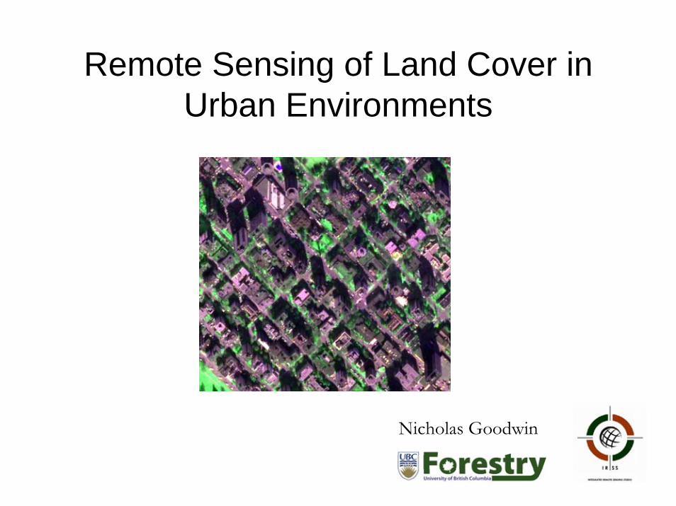
1

Remote Sensing of Land Cover in Urban Environments

Nicholas Goodwin

2

Overview of Topics Covered

• Description of the frequently used satellite sensors for land use mapping

• Applications of satellite imagery for land use mapping

• LiDAR technology and urban applications

3

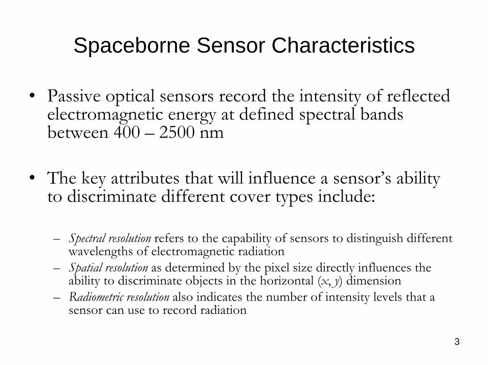
Spaceborne Sensor Characteristics

• Passive optical sensors record the intensity of reflected electromagnetic energy at defined spectral bands between 400 – 2500 nm

• The key attributes that will influence a sensor’s ability to discriminate different cover types include:

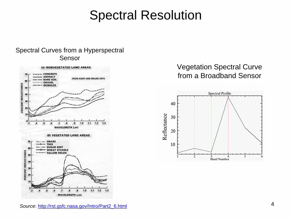
– Spectral resolution refers to the capability of sensors to distinguish different wavelengths of electromagnetic radiation

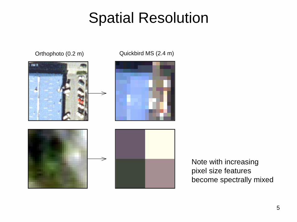
– Spatial resolution as determined by the pixel size directly influences the ability to discriminate objects in the horizontal (x, y) dimension

– Radiometric resolution also indicates the number of intensity levels that a sensor can use to record radiation

4

Spectral Resolution

Spectral Curves from a HyperspectralSensor

Vegetation Spectral Curve from a Broadband Sensor

Source: http://rst.gsfc.nasa.gov/Intro/Part2_6.html

5

Spatial Resolution

Quickbird MS (2.4 m)Orthophoto (0.2 m)

Note with increasing pixel size features become spectrally mixed

6

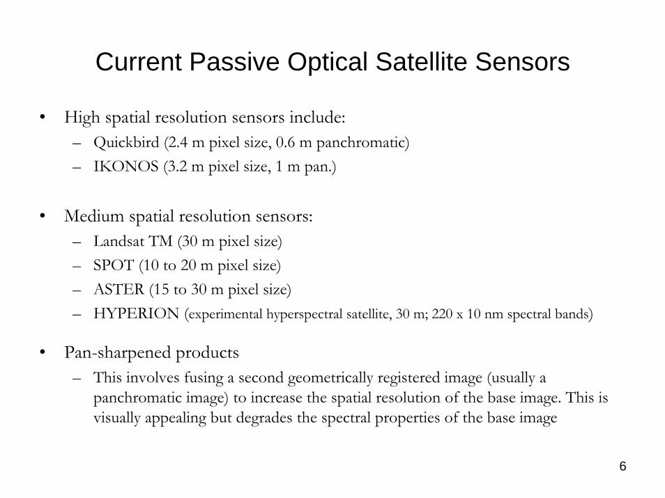
Current Passive Optical Satellite Sensors

• High spatial resolution sensors include:– Quickbird (2.4 m pixel size, 0.6 m panchromatic)– IKONOS (3.2 m pixel size, 1 m pan.)

• Medium spatial resolution sensors:– Landsat TM (30 m pixel size)– SPOT (10 to 20 m pixel size)– ASTER (15 to 30 m pixel size)– HYPERION (experimental hyperspectral satellite, 30 m; 220 x 10 nm spectral bands)

• Pan-sharpened products – This involves fusing a second geometrically registered image (usually a

panchromatic image) to increase the spatial resolution of the base image. This is visually appealing but degrades the spectral properties of the base image

7

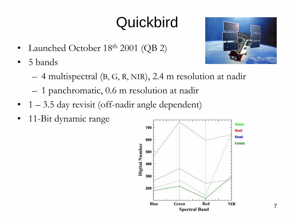
Quickbird• Launched October 18th 2001 (QB 2)• 5 bands

– 4 multispectral (B, G, R, NIR), 2.4 m resolution at nadir– 1 panchromatic, 0.6 m resolution at nadir

• 1 – 3.5 day revisit (off-nadir angle dependent)• 11-Bit dynamic range

8

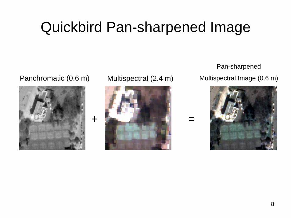
Quickbird Pan-sharpened Image

Pan-sharpened

Multispectral Image (0.6 m)Panchromatic (0.6 m) Multispectral (2.4 m)

+ =

9

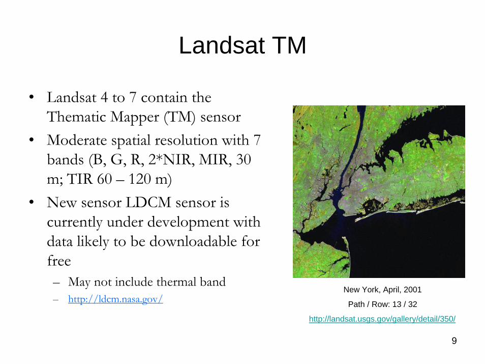
Landsat TM

• Landsat 4 to 7 contain the Thematic Mapper (TM) sensor

• Moderate spatial resolution with 7 bands (B, G, R, 2*NIR, MIR, 30 m; TIR 60 – 120 m)

• New sensor LDCM sensor is currently under development with data likely to be downloadable for free– May not include thermal band– http://ldcm.nasa.gov/

New York, April, 2001

Path / Row: 13 / 32

http://landsat.usgs.gov/gallery/detail/350/

10

Urban Applications of Passive Optical Remote Sensing

• By analysing the spatial patterns in the reflectance of individual bands or band combinations land-use may be assessed over large geographic areas. For example, research has explored the potential to:

– Estimate building area• Classification of buildings based on their reflectance and spatial properties

– eCognition software may be a useful tool to achieve this• Fusion with existing GIS data might also enable more accurate building detection (Mesev, 2007)

– Classification of roof materials • Challenging task due to the wide range of materials that may be used, steep roof

geometry, as well as variability in the spectral properties of target surfaces (different levels of age/wear, dust, moss etc)

• Hyperspectral data from airborne sensors will improve the accuracy of land cover analysis due to a larger number of spectral bands and higher signal to noise ratio

– Derive maps for micrometeorological modeling• For example, populating established climate models (TEB, ISBA) with remote sensing data

regarding building height, building density, vegetation, etc., in order to more efficiently and accurately model the urban climate (Lemonsu et al. 2006)

11

Urban Applications of Passive Optical Remote Sensing (cont.)

– Quantify the fractional abundance (%) of basic surface types within pixels. This is achieved primarily with a technique known as linear spectral unmixing (Small et al. 2006). This surface types might include:

– Impermeable surfaces (roads, roof tops)– Green and non-photosynthetic vegetation, and – Exposed soil

– Vegetation mapping (species and community)• Accuracy of derived layers will be highly dependent on the spectral differences of the

targeted vegetation types• Attributes such as biomass, leaf area index, and structural complexity have been

estimated in forest environments – more work is needed in urban environments to determine whether these are achieved given the mix of species.

– Assess vegetation health and vigour– May be assessed using ratio’s of red (chlorophyll absorption), near infrared (cellular structure)

or mid-infrared (water absorption) reflectance

12

Airborne LiDAR Technology

• What is LiDAR?– LiDAR = Light Detection And Ranging

• Active form of remote sensing measuring distance to target surfaces using narrow beams of near-infrared light (e.g.1064 nm).

• For terrain mapping applications LiDAR systems are primarily operated on airborne platforms and record discrete return data.– Scanning both across and along track

• Over the last decade significant advances have been made to LiDAR instruments with greater pulse repetition frequencies (>100k / sec) and better characterisation of the returned signal

13

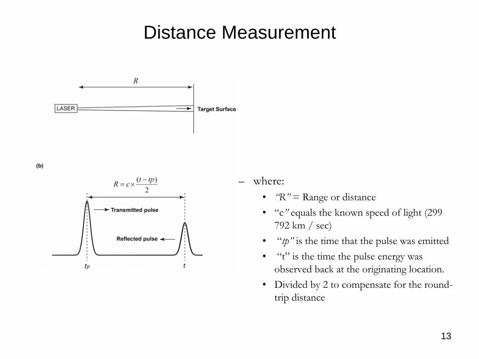
Distance Measurement

– where:• “R” = Range or distance• “c” equals the known speed of light (299

792 km / sec) • “tp” is the time that the pulse was emitted • “t” is the time the pulse energy was

observed back at the originating location. • Divided by 2 to compensate for the round-

trip distance

14

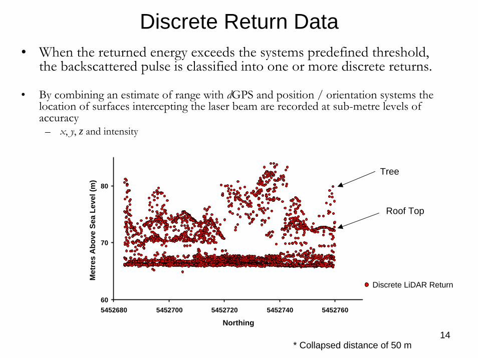
Discrete Return Data• When the returned energy exceeds the systems predefined threshold,

the backscattered pulse is classified into one or more discrete returns.

• By combining an estimate of range with dGPS and position / orientation systems the location of surfaces intercepting the laser beam are recorded at sub-metre levels of accuracy

– x, y, z and intensity

60

70

80

5452680 5452700 5452720 5452740 5452760

Northing

Met

res

Abo

ve S

ea L

evel

(m)

Roof Top

Tree

Discrete LiDAR Return

* Collapsed distance of 50 m

15

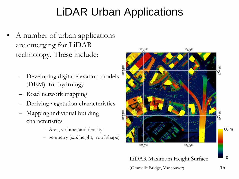
LiDAR Urban Applications

• A number of urban applications are emerging for LiDARtechnology. These include:

– Developing digital elevation models (DEM) for hydrology

– Road network mapping– Deriving vegetation characteristics– Mapping individual building

characteristics– Area, volume, and density– geometry (incl. height, roof shape)

60 m

LiDAR Maximum Height Surface(Granville Bridge, Vancouver)

0

16

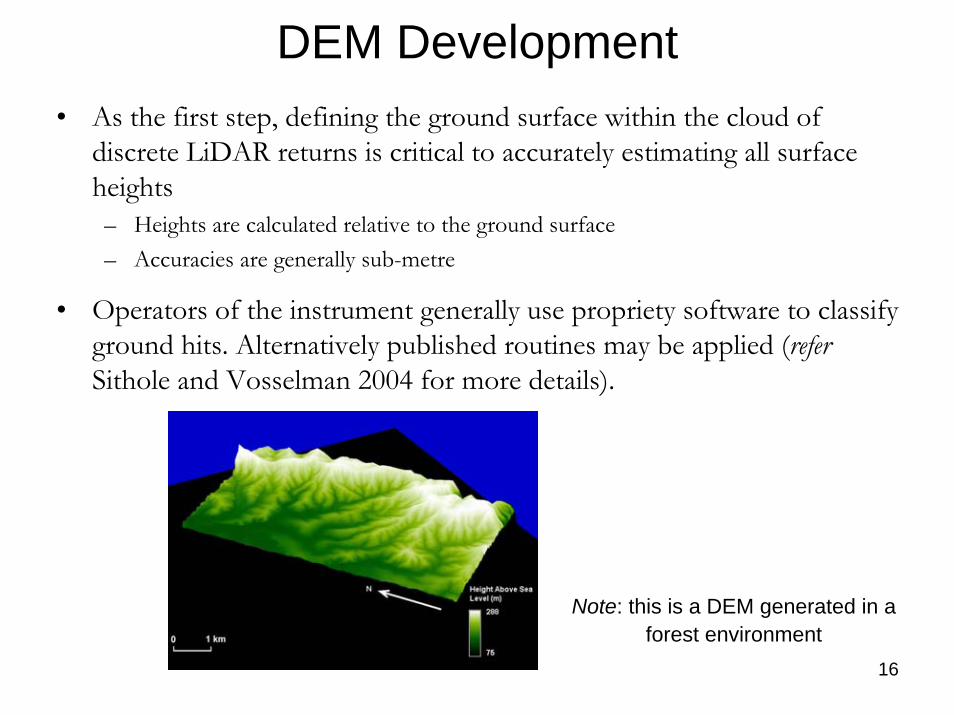
DEM Development• As the first step, defining the ground surface within the cloud of

discrete LiDAR returns is critical to accurately estimating all surface heights– Heights are calculated relative to the ground surface– Accuracies are generally sub-metre

• Operators of the instrument generally use propriety software to classify ground hits. Alternatively published routines may be applied (referSithole and Vosselman 2004 for more details).

Note: this is a DEM generated in a forest environment

17

Approach to Extracting Information on Individual Objects

• Iterative process of examining discrete returns (x,y,z) and interpolated surfaces

• There are some similarities to the analysis of passive optical imagery as they both examine the horizontal patterns within the datasets. However, LiDAR data represents object heights that can be manipulated, whereas passive optical imagery uses reflected light and is pixel based.

• An intensity value is also recorded for each LiDAR return. This is likely to contain useful information but will require calibration as factors such as the orientation of the pulse off-nadir will effect the intensity of the returned signal.

18

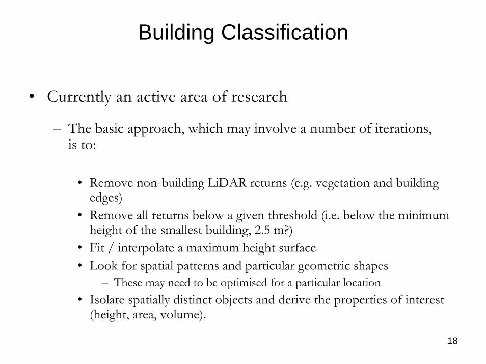
Building Classification

• Currently an active area of research

– The basic approach, which may involve a number of iterations, is to:

• Remove non-building LiDAR returns (e.g. vegetation and building edges)

• Remove all returns below a given threshold (i.e. below the minimum height of the smallest building, 2.5 m?)

• Fit / interpolate a maximum height surface• Look for spatial patterns and particular geometric shapes

– These may need to be optimised for a particular location• Isolate spatially distinct objects and derive the properties of interest

(height, area, volume).

19

Building Delineation

Note: LiDAR delineated building extents are overlaid upon an aerial photograph

Zhang et al. 2006

20

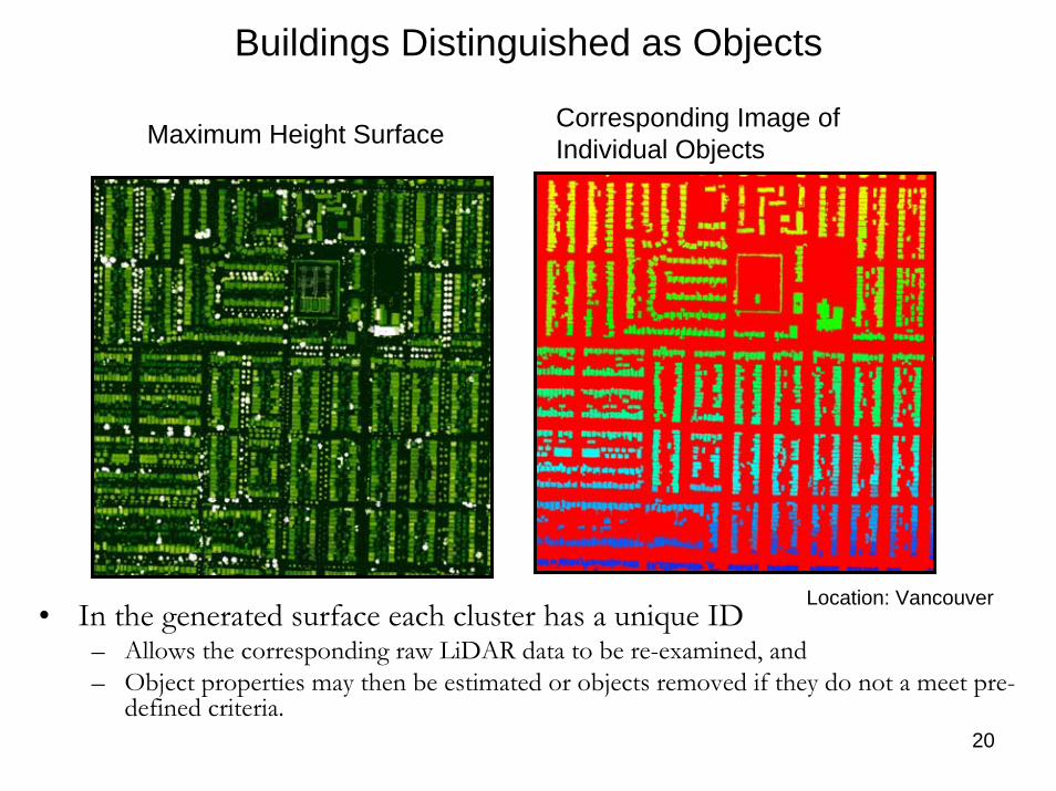
Buildings Distinguished as Objects

Corresponding Image of Individual ObjectsMaximum Height Surface

• In the generated surface each cluster has a unique ID – Allows the corresponding raw LiDAR data to be re-examined, and– Object properties may then be estimated or objects removed if they do not a meet pre-

defined criteria.

Location: Vancouver

21

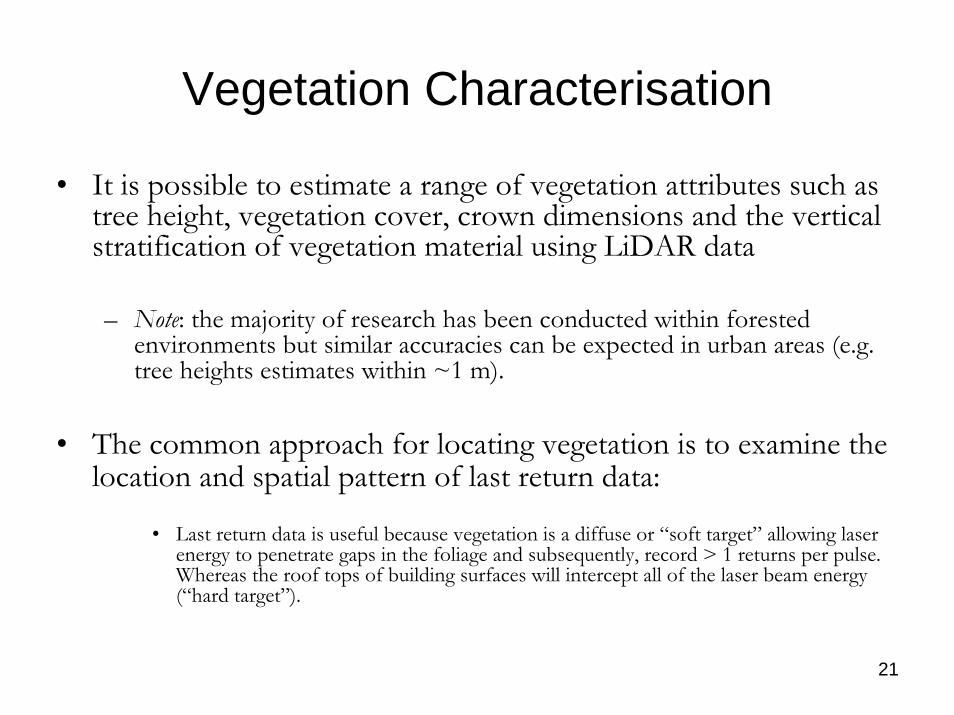
Vegetation Characterisation

• It is possible to estimate a range of vegetation attributes such as tree height, vegetation cover, crown dimensions and the verticalstratification of vegetation material using LiDAR data

– Note: the majority of research has been conducted within forested environments but similar accuracies can be expected in urban areas (e.g. tree heights estimates within ~1 m).

• The common approach for locating vegetation is to examine the location and spatial pattern of last return data:

• Last return data is useful because vegetation is a diffuse or “soft target” allowing laser energy to penetrate gaps in the foliage and subsequently, record > 1 returns per pulse. Whereas the roof tops of building surfaces will intercept all of the laser beam energy (“hard target”).

22

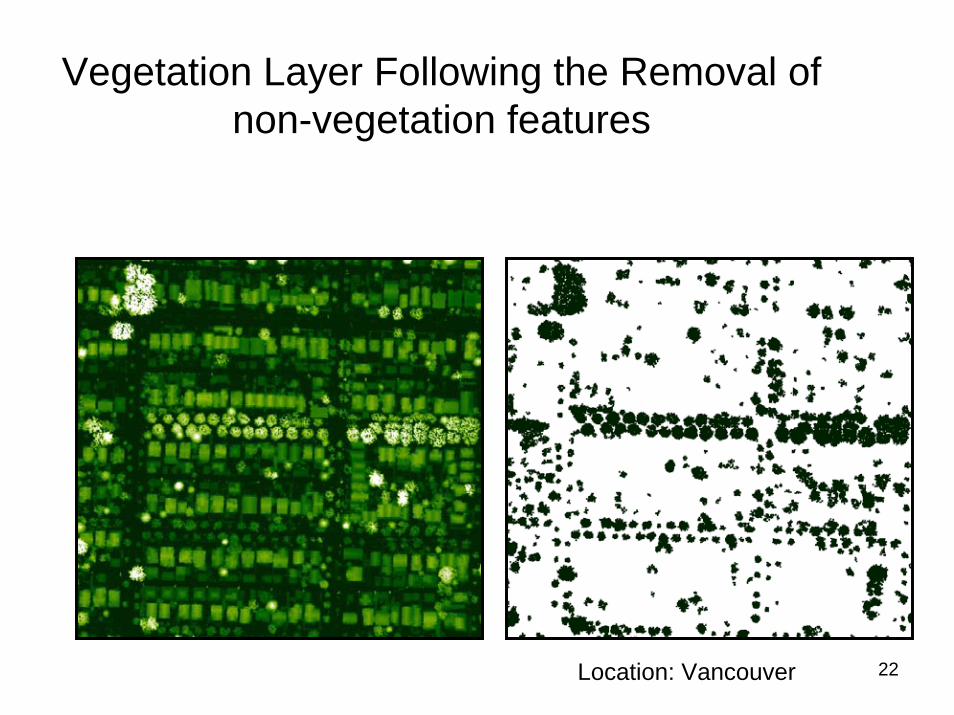
Vegetation Layer Following the Removal of non-vegetation features

Location: Vancouver

23

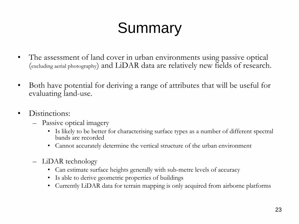
Summary

• The assessment of land cover in urban environments using passive optical (excluding aerial photography) and LiDAR data are relatively new fields of research.

• Both have potential for deriving a range of attributes that will be useful for evaluating land-use.

• Distinctions:– Passive optical imagery

• Is likely to be better for characterising surface types as a number of different spectral bands are recorded

• Cannot accurately determine the vertical structure of the urban environment

– LiDAR technology• Can estimate surface heights generally with sub-metre levels of accuracy• Is able to derive geometric properties of buildings• Currently LiDAR data for terrain mapping is only acquired from airborne platforms

24

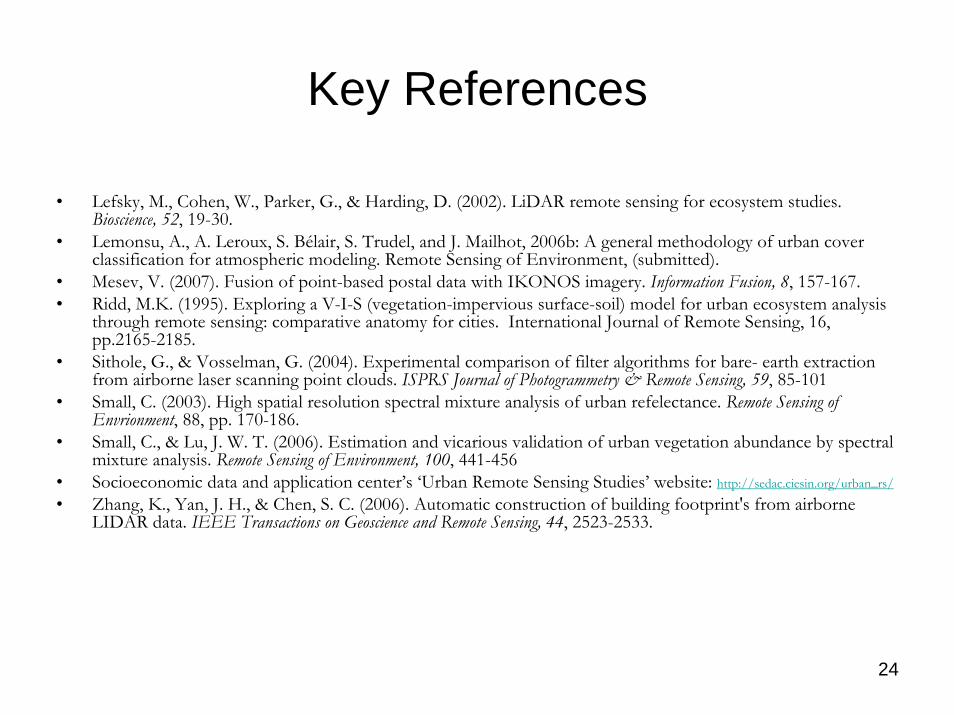
Key References

• Lefsky, M., Cohen, W., Parker, G., & Harding, D. (2002). LiDAR remote sensing for ecosystem studies. Bioscience, 52, 19-30.

• Lemonsu, A., A. Leroux, S. Bélair, S. Trudel, and J. Mailhot, 2006b: A general methodology of urban cover classification for atmospheric modeling. Remote Sensing of Environment, (submitted).

• Mesev, V. (2007). Fusion of point-based postal data with IKONOS imagery. Information Fusion, 8, 157-167.• Ridd, M.K. (1995). Exploring a V-I-S (vegetation-impervious surface-soil) model for urban ecosystem analysis

through remote sensing: comparative anatomy for cities. International Journal of Remote Sensing, 16, pp.2165-2185.

• Sithole, G., & Vosselman, G. (2004). Experimental comparison of filter algorithms for bare- earth extraction from airborne laser scanning point clouds. ISPRS Journal of Photogrammetry & Remote Sensing, 59, 85-101

• Small, C. (2003). High spatial resolution spectral mixture analysis of urban refelectance. Remote Sensing of Envrionment, 88, pp. 170-186.

• Small, C., & Lu, J. W. T. (2006). Estimation and vicarious validation of urban vegetation abundance by spectral mixture analysis. Remote Sensing of Environment, 100, 441-456

• Socioeconomic data and application center’s ‘Urban Remote Sensing Studies’ website: http://sedac.ciesin.org/urban_rs/

• Zhang, K., Yan, J. H., & Chen, S. C. (2006). Automatic construction of building footprint's from airborne LIDAR data. IEEE Transactions on Geoscience and Remote Sensing, 44, 2523-2533.