Embed Size (px)
Citation preview

Relationship between financial ratios and share price performance of the top five
sectors on the Johannesburg Stock Exchange
Peter Desmond Steyn
29040397
A research project submitted to the Gordon Institute of Business Science, University of
Pretoria, in partial fulfilment of the requirements for the degree of Master of Business
Administration.
13 March 2019

i | P a g e
ABSTRACT
Financial ratios have been commonly used to evaluate firm financial performance and
assist investors with the evaluation of shares. Yan and Zheng (2017) argued that the
most important financial ratios are sector specific. The purpose of this research was to
determine if statistically significant relationships exist between financial ratios and the
share price performance of the top five sectors on the Johannesburg Stock Exchange
based on market capitalisation. The five sectors were the mining, banking, life insurance,
real estate investment trusts and mobile telecommunication sectors. Multiple linear
regression as statistical method was applied over a 20-year period from 1997 to 2018.
Statistically significant relationships were found between financial ratios and the share
price performance for each of the five sectors. The mining sector displayed relationships
with return on equity, price-to-book value, debt to equity, dividend yield, debt to assets
and the total asset turnover ratios. Banking displayed relationships with the price-
earnings and return on equity ratios. The life insurance sector and the operating profit
margin displayed a relationship. Lastly, the mobile telecommunication sector delivered
relationships with return on assets, dividend yield and debt to assets. This research
delivered a practical contribution to the theory of quality fundamental analysis from a JSE
sector perspective.

ii | P a g e
KEYWORDS
Financial ratios; Fundamental analysis; Sectors; Share Price; Johannesburg Stock
Exchange (JSE)

iii | P a g e
DECLARATION
I declare that this research project is my own work. It is submitted in partial fulfilment of
the requirements for the degree of Master of Business Administration at the Gordon
Institute of Business Science, University of Pretoria. It has not been submitted before for
any degree or examination in any other University. I further declare that I have obtained
the necessary authorisation and consent to carry out this research.
Peter Desmond Steyn
-------------------------------------------
13 March 2019

iv | P a g e
CONTENTS
ABSTRACT .................................................................................................................... i
KEYWORDS ................................................................................................................. ii
DECLARATION ............................................................................................................ iii
LIST OF TABLES ......................................................................................................... ix
LIST OF FIGURES ........................................................................................................ x
LIST OF EQUATIONS ................................................................................................... x
CHAPTER 1 INTRODUCTION TO RESEARCH PROBLEM .................................... 1
1.1 Research Title ..................................................................................................... 1
1.2 Introduction ......................................................................................................... 1
1.3 Research Problem and Motivation ...................................................................... 1
1.4 Research Objective and Scope ........................................................................... 6
1.5 Academic and Business rationale ....................................................................... 6
1.6 Overview of the research report .......................................................................... 7
CHAPTER 2 LITERATURE REVIEW ....................................................................... 8
2.1 Introduction ......................................................................................................... 8
2.2 Fundamental Analysis ......................................................................................... 8
2.3 Value Investing ..................................................................................................11
2.4 Growth Investing ................................................................................................13
2.5 Financial accounting ratios .................................................................................14
2.5.1 Introduction .................................................................................................14
2.5.2 Liquidity ratios .............................................................................................16
2.5.3 Solvency Ratios ...........................................................................................16
2.5.4 Profitability & Operating Efficiency Ratios ....................................................18
2.5.5 Asset Utilization or Turnover Ratios .............................................................21
2.6 Price-to-fundamental ratios ................................................................................21
2.7 Effect of financial ratios on share price performance ..........................................23
2.8 South Africa, a unique market place ..................................................................28

v | P a g e
2.9 Industries/Sectors of the JSE .............................................................................30
2.10 Conclusion .......................................................................................................32
CHAPTER 3 RESEARCH HYPOTHESES ..............................................................33
3.1 Hypothesis 1: Mining ..........................................................................................34
3.2 Hypothesis 2: Banking .......................................................................................34
3.3 Hypothesis 3: Life Insurance ..............................................................................34
3.4 Hypothesis 4: Real Estate Investment Trusts .....................................................34
3.5 Hypothesis 5: Mobile Telecommunications ........................................................35
CHAPTER 4 RESEARCH METHODOLOGY AND DESIGN ....................................36
4.1 Introduction ........................................................................................................36
4.2 Research Methodology and design ....................................................................36
4.3 Population ..........................................................................................................37
4.4 Unit of analysis ..................................................................................................41
4.5 Sampling method and size .................................................................................42
4.6 Measurement instrument ...................................................................................42
4.7 Data gathering process ......................................................................................44
4.8 Data analysis approach .....................................................................................49
4.8.1 Assumption 1 ..............................................................................................50
4.8.2 Assumption 2 ..............................................................................................50
4.8.3 Assumption 3 ..............................................................................................51
4.8.4 Assumption 4 ..............................................................................................52
4.8.5 Assumption 5 ..............................................................................................52
4.8.6 Assumption 6 ..............................................................................................53
4.8.7 Assumption 7 ..............................................................................................54
4.8.8 Assumption 8 ..............................................................................................55
4.9 Research Ethics .................................................................................................57
4.10 Research Limitations .......................................................................................57
CHAPTER 5 RESULTS ...........................................................................................59
5.1 Introduction ........................................................................................................59

vi | P a g e
5.2 Hypothesis 1: Mining ..........................................................................................59
5.2.1 Description of data obtained and cleaned ....................................................59
5.2.2 Multiple linear regression assumption results ..............................................60
5.2.3 Descriptive statistics ....................................................................................62
5.2.4 Stepwise multiple linear regression results ..................................................63
5.2.5 Result ..........................................................................................................65
5.3 Hypothesis 2: Banking .......................................................................................65
5.3.1 Description of data obtained and cleaned ....................................................65
5.3.2 Multiple linear regression assumption results ..............................................66
5.3.3 Descriptive statistics ....................................................................................68
5.3.4 Stepwise multiple linear regression results ..................................................69
5.3.5 Result ..........................................................................................................70
5.4 Hypothesis 3: Life Insurance ..............................................................................70
5.4.1 Description of data obtained and cleaned ....................................................71
5.4.2 Multiple linear regression assumption results ..............................................71
5.4.3 Descriptive statistics ....................................................................................73
5.4.4 Stepwise multiple linear regression results ..................................................74
5.4.5 Result ..........................................................................................................75
5.5 Hypothesis 4: Real Estate Investment Trusts .....................................................75
5.5.1 Description of data obtained and cleaned ....................................................76
5.5.2 Multiple linear regression assumption results ..............................................76
5.5.3 Descriptive statistics ....................................................................................79
5.5.4 Stepwise multiple linear regression results ..................................................80
5.5.5 Result ..........................................................................................................81
5.6 Hypothesis 5: Mobile Telecommunications ........................................................82
5.6.1 Description of data obtained and cleaned ....................................................82
5.6.2 Multiple linear regression assumption results ..............................................82
5.6.3 Descriptive statistics ....................................................................................84
5.6.4 Stepwise multiple linear regression results ..................................................85
vii | P a g e
5.6.5 Result ..........................................................................................................86
5.7 Summary of results ............................................................................................86
CHAPTER 6 DISCUSSION OF RESULTS ..............................................................88
6.1 Introduction ........................................................................................................88
6.2 Hypothesis 1: Mining ..........................................................................................88
6.3 Hypothesis 2: Banking .......................................................................................91
6.4 Hypothesis 3: Life Insurance ..............................................................................92
6.5 Hypothesis 4: Real Estate Investment Trusts .....................................................93
6.6 Hypothesis 5: Mobile Telecommunications ........................................................94
6.7 Summary of findings ..........................................................................................96
6.7.1 Financial ratio specific .................................................................................96
6.7.2 Country specific ...........................................................................................97
6.7.3 Sector specific .............................................................................................97
CHAPTER 7 CONCLUSION....................................................................................99
7.1 Introduction ........................................................................................................99
7.2 Principal findings .............................................................................................. 100
7.2.1 Financial ratio specific ............................................................................... 101
7.2.2 Country specific ......................................................................................... 101
7.2.3 Sector specific ........................................................................................... 101
7.3 Implications for management ........................................................................... 101
7.3.1 Financial ratio specific ............................................................................... 101
7.3.2 Country specific ......................................................................................... 102
7.3.3 Sector specific ........................................................................................... 102
7.4 Limitations of the research ............................................................................... 103
7.5 Suggestions for future research ....................................................................... 104
7.6 Conclusion ....................................................................................................... 105
REFERENCE LIST .................................................................................................... 106
APPENDIX A: CONSISTENCY MATRIX ................................................................... 118
APPENDIX B: STATISTICAL OUTPUTS PER HYPOTHESIS .................................. 119

viii | P a g e
Hypothesis 1: Mining ............................................................................................. 119
1. Regression Assumptions ............................................................................. 119
2. Automatic Stepwise Regression Outputs .................................................... 133
Hypothesis 2: Banking ........................................................................................... 137
1. Regression Assumptions ............................................................................. 137
2. Automatic Stepwise Regression Outputs .................................................... 145
Hypothesis 3: Life Insurance .................................................................................. 147
1. Regression Assumptions ............................................................................. 147
2. Automatic Stepwise Regression Outputs .................................................... 154
Hypothesis 4: Real Estate Investment Trusts ......................................................... 156
1. Regression Assumptions ............................................................................. 156
2. Automatic Stepwise Regression Outputs .................................................... 165
Hypothesis 5: Mobile Telecommunications ............................................................ 168
1. Regression Assumptions ............................................................................. 168
2. Automatic Stepwise Regression Outputs .................................................... 177

ix | P a g e
LIST OF TABLES
Table 1 Liquidity Ratios ...............................................................................................16
Table 2 Solvency Ratios ..............................................................................................18
Table 3 Profitability & Operating Efficiency Ratios .......................................................21
Table 4 Asset Utilization or Turnover Ratio .................................................................21
Table 5 Price-to-fundamental ratios .............................................................................22
Table 6 Most significant financial ratios per sector ......................................................24
Table 7 Financial ratios and groupings used ...............................................................26
Table 8 Financial Ratios ..............................................................................................33
Table 9 Market capitalisation filters .............................................................................39
Table 10 Top 10 Market Capitalisation per ICB level 3 Sector .....................................40
Table 11 Validity factors and reasoning for each .........................................................43
Table 12 Applied Iress Expert filters ............................................................................45
Table 13 Financial ratios selected ...............................................................................46
Table 14 Financial ratios selected ...............................................................................51
Table 15 Data obtained for mining sector ....................................................................60
Table 16 Descriptive statistics: Mining .........................................................................63
Table 17 Automatic stepwise regression results: Mining .............................................64
Table 18 Data obtained for banking sector ..................................................................66
Table 19 Descriptive statistics: Banking ......................................................................69
Table 20 Automatic stepwise regression results: Banking ...........................................70
Table 21 Data obtained for life insurance sector ..........................................................71
Table 22 Descriptive statistics: Life Insurance .............................................................74
Table 23 Automatic stepwise regression results: Life Insurance ..................................75
Table 24 Data obtained for real estate investment trusts sector ..................................76
Table 25 Descriptive statistics: Real Estate Investment Trusts ....................................80
Table 26 Automatic stepwise regression results: Real Estate Investment Trusts .........81
Table 27 Data obtained for mobile telecommunications sector ....................................82
Table 28 Descriptive statistics: Mobile Telecommunications .......................................85
Table 29 Automatic stepwise regression results: Mobile Telecommunications ............86
Table 30 Summary of stepwise multiple linear regression results ................................87
Table 31 Incomplete datapoints ................................................................................ 104

x | P a g e
LIST OF FIGURES
Figure 1 Portfolio returns for the Levin-Graham stock screen ......................................13
Figure 2 Industry Classification Benchmark .................................................................31
Figure 3 Population funnel ...........................................................................................37
LIST OF EQUATIONS
Equation 1 DuPont analysis ........................................................................................15
Equation 2 Percentage change equation .....................................................................48

1 | P a g e
CHAPTER 1 INTRODUCTION TO RESEARCH PROBLEM
1.1 Research Title
Relationship between financial ratios and share price performance of the top five
sectors on the Johannesburg Stock Exchange.
1.2 Introduction
Delen, Kuzey and Uyar (2013) stated that using financial ratios to evaluate firm
performance and financial health, even though a traditional method, has been a powerful
and important tool for various decision makers. Financial ratio analysis is the most
commonly used and effective financial performance evaluation method (Hsu, 2014;
Musallam, 2018). Financial ratio analysis is also the most informative method of
analysing firm performance due to its ability in delivering insights into every aspect of a
company’s financial performance (Skae et al., 2012).
According to Delen, Kuzey and Uyar (2013), financial ratios have various benefits,
including the measurement of the performance of business managers, measuring the
performance of departments within an organisation and making projections of the future
based on the past. Financial ratios can further be used to perform comparisons with
competitors or other companies across industries (Delen, Kuzey & Uyar, 2013;
Musallam, 2018). Another benefit is that the financial performance of companies of
different sizes can be compared to each other as they are judged on the same scale
(Delen, Kuzey & Uyar, 2013; Yan & Zheng, 2017).
Financial ratios are most commonly used to evaluate financial performance of
organisations in order to determine possible future stock returns (Delen, Kuzey & Uyar,
2013; Musallam, 2018). This is corroborated by Safdar (2016) which states that the
interest in using financial statements in predicting future stock returns has been evident
since the early 1900’s, mainly due to the expectation that financial statement analysis
could be valuable in discovering important information to make superior investment
decisions.
1.3 Research Problem and Motivation
The first problem which however arises from financial ratios, financial ratio-based
evaluation models and financial variables are their abundance and the lack of consensus
regarding which financial ratios are of most importance. Some of the first noticeable
authors identified, which mentioned this, was Ou and Penman (1989) who argued that

2 | P a g e
even though previous academic literature agreed that financial statements were to be
used to perform fundamental and ratio analysis, that little guidance was provided on
which ratios were of most importance and therefore the authors used 68 different
financial ratios in their research performed.
With regard to evaluating financial performance of an organisation, Delen, Kuzey and
Uyar (2013) stated that when searching for literature regarding the use of financial ratios
to evaluate firm performance, that thousands of publications were available, where each
study tried to differentiate themselves by way of developing a different set of financial
ratios. Delen, Kuzey and Uyar (2013) argued that “there is no universally agreed-upon
list regarding the type, calculation methods and number of financial ratios used in earlier
studies” (p. 3971). It was further mentioned that various earlier research used between
15 to nearly 60 different financial ratios.
With regard to stock returns, Yan and Zheng (2017) commented that finance researchers
have sought to determine what the causes of stock return patterns are, which has led to
hundreds of cross-sectional return anomalies being identified and documented. This
abundance is further made clear by Hou, Xue, Zhang (2015), which investigated a broad
range of 80 financial return anomaly variables, of which the majority were financial ratios.
They further mentioned various other researchers which used a varying number of
financial variables of up to 300 in their testing performed. Light, Maslov and Rytchkov
(2017), document other research findings delivering significant financial variables
between 50 and 330 variables.
An extreme example was where Yan and Zheng (2017) applied more than 18 000
financial statement derived fundamental variables, using data mining techniques, to
predict stock returns. Further to this, in addition to financial accounting ratios, investors
use price-to-fundamental ratios for share evaluation purposes. These include the
dividend-yield, price-earnings, price-to-book and price-to-cash flow ratios to name a few
(Chua, Delisle, Feng & Lee, 2014; Fama & French, 2008, 2012; Gupta & Modise, 2012;
Lewellen, 2004; Morar, 2014; Muller & Ward, 2013; Jiang & Lee, 2007). The problem of
abundance, continuous differences in the financial variables used and the results
obtained from these variables therefore still appears to exist.
Consequently, amateur investors and managers with less technical financial knowledge
in some instances, resort to applying and analysing an excess of financial ratios and
financial models in a hopeful attempt to cover the most important. Investors further often
3 | P a g e
suffer from a lack of expertise and end up making the incorrect investment decisions
(Hsu, 2014). Business and finance students are also normally supplied with a list of
financial ratios and financial models from a theoretical perspective, but in some
instances, the specific ones to use which are of most importance in their specific fields
of business or practice, is rather left for self-exploration and interpretation. The
researcher has personally noticed this problem as various business students, studying
towards an MBA, after the completion of their finance and accounting modules, are still
seeking guidance as to which are the main financial ratios which drive their industries.
With so many financial ratios and financial models available, it is sometimes unclear to
less experienced users which are the most important ratios to focus on for a specific
industry or sector in respect of share price performance.
The second problem which arises is the lack of South African financial ratio studies
performed. According to Bunting and Barnard (2015), very few fundamental analysis
studies have been performed outside the United States (U.S.) equity markets. Bunting
and Barnard (2015) further noted that various differences exist between the United
States accounting standards, security regulations and market microstructure when
compared to other countries. The United States uses U.S. Generally Accepted
Accounting Principles (GAAP) as accounting standard, where South Africa, uses
International Financial Reporting Standards (IFRS) (Barth, Landsman, Lang & Williams,
2012; IFRS, 2016). Barth, Landsman, Lang and Williams (2012) argued that significant
differences exist between the two accounting standards. Cinca, Molinero, and Larraz
(2005) further determined that the countries where companies are located impact the
structures of their financial ratios. These differences provide sufficient evidence to
question if financial ratio models developed based on U.S. data would be transportable
and replicable in the South African context with similar findings achieved (Bunting and
Barnard, 2015).
Further to this, more recent literature by Konku, Rayhorn, and Yao (2018) argued that
most of the research on stock price behaviour has focussed on developed markets, as
data was more easily obtainable. They stated that emerging market economies have
gained significant growth in the last two decades and therefore the importance for
investors have started to increase. According to Financial Times (n.d.) “Emerging market
is a term that investors use to describe a developing country, in which investment would
be expected to achieve higher returns but be accompanied by greater risk” (para. 1).
According to Konku, Rayhorn, and Yao (2018) the emerging market focus has been
mainly based on larger emerging markets including Brazil, Russia, India and China, but
4 | P a g e
the focus was turning to smaller emerging economies like South Africa due to the desire
of diversification by developed country investors and the potential for higher returns. The
authors further argued that studies on African markets were not as abundant as those of
other emerging markets.
Deloitte (2017) argued that when South Africa was included as part of the BRICS (Brazil,
Russia, India, China and South Africa) acronym in 2010, and was regarded as a first-tier
emerging market, that all the BRICS nations were regarded as performing well in terms
of rising and future demand. The BRICS landscape has however changed. While the
Chinese and Indian emerging economies are growing and could deliver the higher
returns as expected by emerging markets, South Africa is starting to display the bad
economic trends of Brazil. With various credit rating downgrades (BB+ in 2017), various
quarters of negative GDP growth realised in the most recent years, an unstable political
environment, public sector underperformance and reduced investor confidence, South
Africa might not deliver the higher returns which are expected from emerging markets.
The results achieved from other emerging market finance research performed, might
therefore not be replicable on the South African equity markets when attempted. It
therefore appears that the South African economic and equity market landscape is
unique to those of developed markets and some of those classified as emerging markets.
The third problem noted is that even though some South African specific financial ratio
and share return related studies have been performed, that those identified by the
researcher have been performed under a different lens. None of these focussed on the
different sectors present on the Johannesburg Stock Exchange (JSE) in isolation. Yan
and Zheng (2017) argued that the most important financial ratios are industry specific.
Safdar (2016) further placed emphasis on the importance of industry context when
performing financial ratio analysis and argued that financial ratio based fundamental
analysis is more effective when used in industries which have less competition.
Delen, Kuzey and Uyar (2013) stated that the financial ratio structures of manufacturing
and retail firms are different. Mohanram, Saiy, and Vyas (2018) further argued that most
financial statement-based research performed excludes bank stocks, as banks have
vastly different financial drivers when compared to other industries. This literature
provides substantial evidence that most sectors are unique as they have different
financial drivers, financial structures and different market dynamics. More specific and
focussed results could therefore be derived and would be beneficial, if a sector specific
study is performed.

5 | P a g e
The first South African study reviewed was that of Gupta and Modise (2012), where only
two pricing ratios, namely the price-earnings and price-dividend ratios were evaluated
for their share return predictability capabilities in the South African context over a period
of nearly 20 years. This was followed by Hoffman (2012), which through the inclusion of
all the companies listed on the JSE (376 companies) in aggregate, determined the effect
that a few explanatory variables, including some financial ratios and other factors, have
on stock returns. Next was the research by Muller and Ward (2013) which sought to
determine the best financial ratio and other factor investing styles to use on the JSE. The
top 160 companies of the Johannesburg Stock Exchange based on market capitalisation
were researched over a 27-year period.
Ramkillawan (2014) further sought to determine what the relationships of only two
financial accounting ratios were with the average stock returns of the Top 40 index of the
Johannesburg Stock Exchange and the Top 50 index of the Nigerian Stock Exchange.
This was followed by Morar (2014), which focussed on BRICS stock exchanges, but only
applied four price-to-fundamental financial ratios in an attempted model for stock
selection which only ranged over a period three years. The last study was that of Bunting
and Barnard (2015), where a South African JSE based Piotroski F-Score study was
performed to determine the relationship between financial accounting ratios and equity
returns.
None of the above South African based or inclusive studies mentioned, focussed on the
different South African JSE sectors in isolation, but grouped all companies from different
sectors together during these evaluations. The only study which took some cognisance
of the industries was that of Muller and Ward (2013), but an analysis was only performed
between the high level industrial and resource classifications on the JSE to determine
which of these two industries delivered the highest returns. By referring to the lowest
level of the Industry Classification Benchmark (ICB) which is used by the JSE, 114
subsectors exist which provides an indication of how many classification categories are
available in which companies on the JSE can be classified (FTSE Russell, n.d.).
Some researchers in other areas of the world, which have performed sector-based
studies, have found stronger relationships between financial ratios and share price
performance in certain sectors when compared to others. Vedd and Yassinski (2015),
through analysing the Latin American industrial sector, determined that the asset
turnover ratio and share prices in Brazil, Chile and Mexico were strongly correlated. Ma
6 | P a g e
and Truong (2015), through an analysis of the banking, energy, investment, real estate
and retail sectors of the Swedish OMX stock exchange, determined that the financial
ratios which affect share price movement the most for each sector, was industry specific.
From the results obtained by international sector-based studies, a clear argument can
be made that more value could be derived by evaluating financial ratios and share price
performance on a sector basis in the South African context instead of merely grouping
all the companies together. The question which emerges from the combination of the
three problems identified, is if financial ratios have statistical relationships with the share
price performance of the different sectors of the South African JSE.
1.4 Research Objective and Scope
The objective of this research was to determine if statistically significant relationships
exist between financial ratios and share price performance of different sectors on the
JSE, with the possible result that the main financial ratio drivers of each sectors share
price could be determined. To the best of the researcher’s knowledge, a sector-based
study regarding the relationship between financial ratios and share price performance
has not been performed in the South African JSE market space. The scope of this
research includes the top five sectors of the JSE based on the combined market
capitalisation of each sector.
The sectors were classified according to the third level classification of the Industry
Classification Benchmark (ICB) of which 41 sectors were available (FTSE Russell, n.d.).
A broad range of fourteen specific financial ratios were used in the multiple linear
regression analysis performed, including both those from a financial accounting and
price-to-fundamental ratio perspective in order to form a holistic representation of the
most important financial ratios for each sector. The scope of the research further ranged
over a comparative period of 20 years from 1997 to 2018 with 1997 being set as the
base year. This research aimed to deliver a practical contribution to the theory of quality
fundamental analysis from a South African Johannesburg Stock Exchange sector
perspective.
1.5 Academic and Business rationale
This research aimed to provide investors targeting certain sectors of the JSE greater
insight regarding the specific financial ratios to focus on when evaluating equity shares
for purchase in the different sectors included in the scope. This research further aimed
to provide managers or executives operating in the selected sectors guidance as to
which financial ratios are of most importance to their organisations when attempting to

7 | P a g e
drive share price performance. Further, the aim was to assist these parties during
decision making, as the possible effect on share price might be more predictable when
for example making decisions regarding the organisations debt to equity structures or
dividend policies. Lastly, this study aimed to aid finance, investment and accounting
academic literature in South Africa, to improve the student’s understanding regarding
financial ratios and their relationship with share price performance in the various sectors
included in the scope.
1.6 Overview of the research report
Chapter 2 follows and delves into the body of literature surrounding financial ratio-based
company performance analysis, investment techniques commonly used and the detail
around the different types of financial ratios. Further, Chapter 2 discusses what other
researchers have found regarding the effect of financial ratios on share price
performance and justifies the validity of performing this research on a sector basis on
the South African JSE. Chapter 3 provides the hypotheses as determined from the
research question and literature reviewed. Chapter 4 provides the methodology and
design of the research project and the initial limitations identified before the data
processing was performed. Chapter 5 provides the results of the data analysis as
performed in accordance with the methodology and design documented in Chapter 4.
Chapter 6 then discusses the results of Chapter 5 in the context of the literature reviewed
in Chapter 2 and further provides the integrated findings derived from the individual
hypothesis results and related literature. Lastly, Chapter 7 provides a conclusion of the
research project performed, summarising the principal findings derived from Chapter 6,
stating the implications for management, indicating the limitations encountered during
the research and providing suggestions for future research.

8 | P a g e
CHAPTER 2 LITERATURE REVIEW
2.1 Introduction
The purpose of this research was to determine if financial ratios have statistical
relationships with the share price performance of the top five sectors of the JSE, based
on market capitalisation. The literature review aimed to uncover the academic theory,
debates and findings which assisted in framing the research hypotheses. Firstly, some
of the most common theories and methods which investors use to evaluate shares were
reviewed. From this literature the most important financial ratio classification groups were
identified. These classification groups were individually investigated. The effects of the
above financial ratios, identified from the classification groups, on share prices were
reviewed. South Africa’s positioning in the global economy and the Johannesburg Stock
Exchange’s positioning among the global equity markets were then reviewed. A review
of the industry and sector classification standards, as used by the JSE, was lastly
performed. The literature review was then concluded with the main findings which lead
to the research hypotheses in Chapter 3.
2.2 Fundamental Analysis
It is generally accepted that two types of investing techniques exist, namely technical
analysis and fundamental analysis (Avramov, Kaplanski & Levy, 2018; Chen, Lee & Shih,
2016). Technical analysis is normally used by technical security analysts and share
portfolio managers where their main focus is on short-term price gains and volumes
traded, identified with the use of charts (Avramov, Kaplanski & Levy, 2018; Chen, Lee &
Shih, 2016). Hoffmann and Shefrin (2014) found that investors which operate on an
individual basis and make use of technical analysis perform poorly when compared to
other individual investors. Fundamental analysis on the other end considers firm-specific
financial statements, the industry, the market, and firm-level economic factors to name
a few (Avramov, Kaplanski & Levy, 2018; Chen, Lee & Shih, 2016). This research follows
a fundamental analysis approach as this approach relies on financial ratios, which have
a wide application for various users including business managers, investors and
business students. This approach was best suited for the research performed.
According to Li and Mohanram (2018) and Bartram and Grinblatt (2018), the main
concept of fundamental analysis is that a stock might currently be mispriced, but it is
expected to correct itself in the future to reflect the fundamental value of the stock.
Investors thereby make profits by purchasing these mispriced stocks at the low prices
and selling them when the market corrects itself. Li and Mohanram (2018) stated that

9 | P a g e
there are two approaches to fundamental analysis. The value approach is the first, where
the stock’s inherent value is determined based on the application of valuation techniques.
Stock will only then be purchased if this inherent value is more than the market price that
the stock is currently being traded for (Li & Mohanram, 2018). Various valuation methods
to calculate the inherent value of a stock exists, but to obtain the value, highly stylized
fair value models are needed, such as the discounted cash flow model, where future
earnings, cash flow forecasts, discount rates and growth rates are required (Bartram &
Grinblatt, 2018; Li & Mohanram, 2018). The issue with this method is that forecasts are
merely subjective estimations, based on opinions and speculation (Lee, 2014; Li &
Mohanram, 2018). These valuation methods further rely on summary metrics such as
book value, earnings, cash flow and dividends and therefore only partially utilise the rich
information available in the financial statements (Li & Mohanram, 2018).
According to Li and Mohanram (2018), the second approach is the quality approach,
where financial statements are used to identify organisations with strong fundamentals,
that are expected to deliver good performance in the future and generate high returns.
The quality approach uses the rich information which is contained in the financial
statements and therefore can be applied to more companies (Li & Mohanram, 2018).
The study performed by the researcher used financial ratio analysis as derived from
financial statements and market information and therefore was classified as part of the
quality fundamental analysis approach.
The effectiveness of the quality approach was substantiated in various earlier research
performed. Some of the first notable research into the quality approach was performed
by Ou and Penman (1989) where the authors stated that an organisation’s value is
determined by the information contained in the financial statements. The authors
believed that values that are not reflected in the share prices could be detected by
analysing the financial statements. With the use of 68 financial ratios, Ou and Penman
(1989) were able to determine that financial statement analysis can predict future stock
returns.
Piotroski (2000) developed a fundamental analysis strategy, where nine simple
accounting fundamental signals were used to form a combined F-Score. If a share
complied with a fundamental signal requirement, it would be awarded a score (F-Score)
for each of the nine requirements. Shares would then be classified in groups based on
their F-Scores and would be analysed against their stock returns. Four of the nine signals
related to profitability, three of the nine signals related to solvency and liquidity and two

10 | P a g e
of the nine signals related to operating efficiency. All these ratios were calculated from
the companies’ financial statements. These classifications were corroborated by Muller
and Ward (2013) which stated that the classification of the F-score variables took the
form of the DuPont ratio analysis, as discussed in section 2.5.1. It was determined that
when the F-Score method was applied to portfolios of high book-to-market firms (value
stocks) that stocks could be selected which delivered significant stock returns. This fact
was further substantiated by Bunting and Barnard (2015), Chen, Lee and Shih (2016),
Li and Mohanram, (2018), Safdar (2016) and Turtle and Wang (2017) to name a few.
Mohanram (2005) took a similar approach to that of Piotroski (2000) and developed a G-
Score model, consisting of eight fundamental signals, which could be applied to low
book-to-market stocks, classified as growth stocks. The first three of the eight signals
related to the profitability of an organisation. The next two signals related to the stability
of growth ratios. The final three of the eight ratios related to ratios that would affect
current profitability negatively, but boost future growth ratios of a company, thereby
investing current profits for future growth. Mohanram (2005) determined that when the
G-Score approach was applied to portfolios of growth stocks, in the long and short term,
that significant excess stock returns could be realised. Piotroski and So (2012) later
determined that the F-Score strategy, as developed in Piotroski (2000), was not only
applicable to high book-to-market stocks but also was useful when applied to a broad
variety of stocks.
Due to the nature of pure quality driven financial statement based fundamental analysis,
none of the above studies performed incorporated price or market ratios, but only
included ratios developed purely from financial statements. One important aspect
however determined from these quality fundamental analysis studies, was that the ratios
included generally fell under the categories of liquidity, solvency, profitability, operating
efficiency and asset utilization (Delen, Kuzey & Uyar, 2013; Musallam, 2018). These
financial accounting ratio classifications groups and their meanings were therefore
further explored in section 2.5.
Even though some of these studies and underlying theories are a bit dated, they are
widely used as a basis for research, further exploration or form part of the academic
literature in new developing theories (Bartram & Grinblatt, 2018; Bin, Chen, Puclik, & Su,
2017; Bunting & Barnard, 2015; Chen, Lee & Shih, 2016; Goodman, Neamtiu & Zhang,
2018; Hou, Xue & Zhang, 2015; Kim & Lee, 2014; Li & Mohanram, 2018; Mohanram,

11 | P a g e
Saiy & Vyas, 2018; Morar, 2014; Muller & Ward, 2013; Richardson, Tuna & Wysocki,
2010; Safdar, 2016; Turtle & Wang, 2017).
Some of the latest research have used the quality F-Score and G-Score methods in
combination with other approaches including the value approach in Li and Mohanram
(2018) and the technical analysis approach in Chen, Lee and Shih (2016) in order to
determine if combinations of these methods, with others, could lead to improved returns.
Chen, Lee and Shih (2016) found that when the F-Score and the G-Score methods are
applied in combination, that an investment strategy was obtained that delivered
significant stock returns. These theories are therefore still very relevant and are being
researched more widely in various configurations on a developed market basis.
2.3 Value Investing
Value investing is not a new concept and was grounded in 1934 with the book by
Benjamin Graham and David Dodd, titled “Security Analysis”, opening the field of buying
under-priced shares based on fundamental analysis (Asness, Frazzini, Israel &
Moskowitz, 2015; Lee, 2014; Li & Mohanram, 2018; Muller & Ward, 2013). The concept
of value investing has been used by some of the greatest investors in the world, including
Warren Buffet to the point where he posted a foreword in the latest publication of the
series in 2008 (Graham & Dodd, 2008; Lee, 2014).
According to Athanassakos (2012), value investing involves a three-step process. Firstly,
the market is scanned for potentially under-priced stocks. Various price-to-fundamental
ratio screens are used for the screening process including the price-earnings (P/E),
price-to-book (P/B), cash flow-to-price, earnings yield (Inverse of P/E) and dividend yield
(DY) (Asness, Frazzini, Israel & Moskowitz, 2015; Athanassakos, 2012; Bartram &
Grinblatt, 2018; Chen, 2017; Lee, 2014; Li & Mohanram, 2018; Penman & Reggiani,
2018; Piotroski & So, 2012; Richardson, Tuna & Wysocki, 2010). Secondly, after the
stocks have been screened, the stocks identified which seems to be under-priced, are
evaluated more in-depth based on the fundamental analysis approaches discussed
earlier to determine the value (Athanassakos, 2012). Lastly when a stock appears to
have a higher value than its current market price, a decision is made whether the stock
is to be purchased or not. Athanassakos (2012) argued that some investors only use the
first step of value investing where they apply screens to stocks to invest in without much
further consideration. Value stocks tend to pay more dividends, when compared to those
of growth stocks (discussed in 2.4) and therefore reliable dividend track records are of
importance to many value investors (Chen, 2018; Conover, Jensen & Simpson, 2016).

12 | P a g e
Lee (2014) and Li and Mohanram (2018) used versions of Graham’s value investing
screens in their research. Graham’s value investing screens included a total of 10
screens of which the first five measured the relative cheapness of the stock and included
various price and price-to-fundamental ratios (Lee, 2014). The second grouping of five
ratios did not include any pricing ratios and were purely based on information derived
from financial statements in order to form an opinion on the quality of the company (Lee,
2014). The 10 screens in totality therefore included both price-to-fundamental and
financial accounting ratios.
In Lee (2014), a slightly adapted version of these 10 screens, referred to as the “Levin-
Graham strategy”, was applied to U.S. companies for a period of 14 years ranging from
1999 to 2013. Dividend yield was replaced by cash-flow yield and the 10 years of
earnings was replaced with five years. If a company met a condition, then a “+1” was
allocated to it. If a company met all 10 screening conditions, then a “+10” was given and
so forth. All these companies with their scores from 1 to 10 were then grouped into
portfolios ranging from 0-100. The “0-10” portfolio included the companies which had a
“+1” score, the “10-20” portfolio included those with a “+2” score and so forth. The
average returns generated by these 10 portfolios of stocks, which were determined on a
quarterly rebalanced, equal weighted basis, were then compared to the average return
on the Standard & Poor’s (S&P) Dow Jones Midcap 400 index indicated in the first
column of Figure 1. The Standard & Poor’s (S&P) Dow Jones Midcap 400 index is the
top 400 mid-sized market capitalisation ranked companies on the NYSE or NASDAQ. It
was determined that these value investing screens, even though based on historical
principles, still carried immense value as shown in Figure 1 (Lee, 2014).

13 | P a g e
Figure 1. Portfolio returns for the Levin-Graham stock screen test period 1999 to 2013
(Lee, 2014).
Figure 1 clearly shows that by combining financial accounting ratios and price-to-
fundamental ratios, that more value could be derived for analysis and research purposes
as investors are expected to make use of both. This is further corroborated by Bartram
and Grinblatt (2018) which stated that various finance research uses information and
ratios from the financial statements, and price-to-fundamental ratios to predict stock
returns. Seeing the importance of both categories, financial accounting ratios (2.5) and
price-to-fundamental ratios (2.6) were further reviewed in the sections indicated.
2.4 Growth Investing
As discussed in the section 2.3, value investors normally tend to choose stocks with low
price-to-fundamental ratios (or the inverse, high fundamental-to-price ratios) as they are
cautious to overpay for stock (Athanassakos, 2012; Chen, 2017; Hou, Xue & Zhang,
2015; Muller & Ward, 2013; Penman & Reggiani, 2018; Richardson, Tuna & Wysocki,
2010; Zhang, 2013). Growth stocks, on the other side, normally have high price-to-
fundamental ratios, of which the most common identifiers are high price-to-book ratios
(or the inverse, low book-to-market ratios) and high price-earnings (P/E) ratios

14 | P a g e
(Athanassakos, 2012; Bunting & Barnard, 2015; Chen, 2017; Hou, Xue & Zhang, 2015;
Li & Mohanram, 2018; Mohanram, 2005; Muller & Ward, 2013; Penman & Reggiani,
2018; Richardson, Tuna & Wysocki, 2010; Zhang, 2013).
Growth investors anticipate that the growth of growth stocks will be significantly higher
than the average market growth and thereby focus on earning profits through capital
gains when the stocks are sold (Chen, 2018). Dividends are therefore not normally paid
by growth stocks as cash flows generated are mostly reinvested by the companies in
order to increase growth in the short term (Chen, 2018; Conover, Jensen & Simpson,
2016). Growth investors therefore do not place much value on dividends (Conover,
Jensen & Simpson, 2016). Value stocks normally have high dividend yields, where
growth stocks tend to have low dividend yields (Conover, Jensen & Simpson, 2016).
Growth stocks normally tend to be overvalued as the prices seem to be driven by
excitement in recent market performance and optimistic expectations rather than by the
fundamentals of the company (Chen, 2018; Mohanram, 2005; Piotroski & So, 2012). This
method of investing is therefore very risky, because if the optimistic growth as expected
by investors is not realised, losses could be incurred when the stocks are sold which is
further combined with the receival of no dividends (Chen, 2018). Conover, Jensen and
Simpson (2016) and Cordis (2014) found that value stocks which normally have low
price-to-book ratios and high dividend yields, have higher returns when compared to
growth stocks.
In summary, it is therefore important to note that even though low price-to-fundamental
ratios, especially a P/E and P/B ratio combined with a strong track record of dividend
payments might be preferred by some investors, which classify themselves as value
investors, growth investors might not focus on these ratios, and would be willing to
purchase shares with high price-to-fundamental ratios and no dividends (Chen, 2018;
Conover, Jensen & Simpson, 2016). Various investors however include both types of
stocks in their portfolios for risk diversification purposes (Chen, 2018).
2.5 Financial accounting ratios
2.5.1 Introduction
According to Yan and Zheng (2017), more meaning can be derived from financial
statements, if one variable in the financial statements is compared to another, where this
comparison forms financial ratios. Financial ratios are valuable tools for various reasons
15 | P a g e
of which one is that the financial health of an organisation can be analysed (Delen, Kuzey
& Uyar, 2013; Musallam, 2018). Financial ratio analysis is the most informative financial
statement analysis method due to its capability of analysing every aspect of an
organisation’s financial position (Skae et al., 2012).
Managers and users of financial ratios should however be aware that financial ratios on
a standalone basis do not always provide as much value, but become much more
valuable if tracked over time and in addition are compared to industry standards
(Financial ratios, n.d.; Musallam, 2018). Financial accounting ratios can be classified into
various groupings namely liquidity, solvency, profitability (operating efficiency), asset
utilization or turnover ratios of which a discussion of each follows in the sections below
(Delen, Kuzey & Uyar, 2013; Musallam, 2018).
A useful and widely used tool which has assisted various financial statement users with
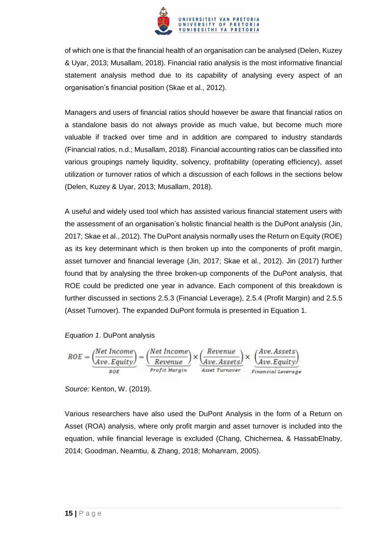
the assessment of an organisation’s holistic financial health is the DuPont analysis (Jin,
2017; Skae et al., 2012). The DuPont analysis normally uses the Return on Equity (ROE)
as its key determinant which is then broken up into the components of profit margin,
asset turnover and financial leverage (Jin, 2017; Skae et al., 2012). Jin (2017) further
found that by analysing the three broken-up components of the DuPont analysis, that
ROE could be predicted one year in advance. Each component of this breakdown is
further discussed in sections 2.5.3 (Financial Leverage), 2.5.4 (Profit Margin) and 2.5.5
(Asset Turnover). The expanded DuPont formula is presented in Equation 1.
Equation 1. DuPont analysis
Source: Kenton, W. (2019).
Various researchers have also used the DuPont Analysis in the form of a Return on
Asset (ROA) analysis, where only profit margin and asset turnover is included into the
equation, while financial leverage is excluded (Chang, Chichernea, & HassabElnaby,
2014; Goodman, Neamtiu, & Zhang, 2018; Mohanram, 2005).
16 | P a g e
2.5.2 Liquidity ratios
These ratios are used to measure an organisation’s ability to cover its current liabilities
or payment obligations, using its cash and other current assets, such as inventory and
receivables, which are quickly convertible into cash (BDO, 2017; Khidmat & Rehman,
2014; Ehiedu, 2014). Liquidity of an organisation is important as a company normally
converts its current assets, as it is more liquid than long term-assets, to obtain cash,
which is then used to cover the current liabilities (Skae et al., 2012). Ehiedu (2014)
argued that liquidity is crucial to the existence and operation of a company. Liquidity is
affected by the operating cash flows generated by a company’s assets (Khidmat &
Rehman, 2014). A few variations of these liquidity ratios exist of which the main ratios
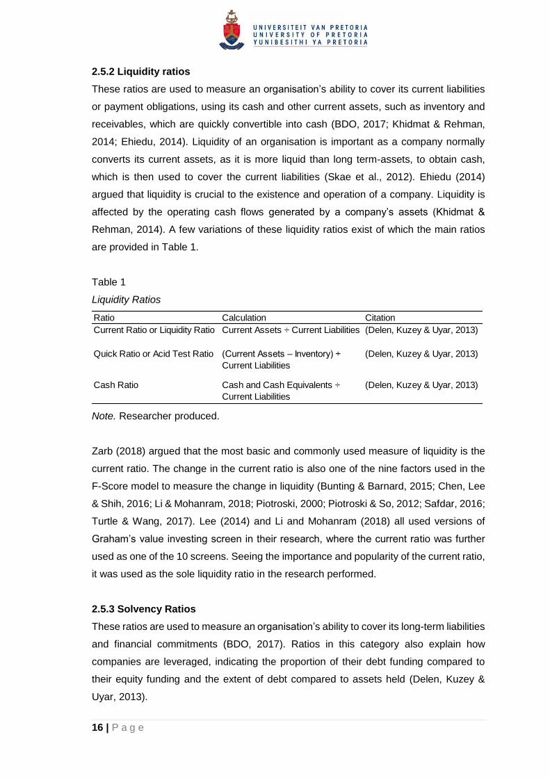
are provided in Table 1.
Table 1 Liquidity Ratios
Liquidity Ratios
Note. Researcher produced.
Zarb (2018) argued that the most basic and commonly used measure of liquidity is the
current ratio. The change in the current ratio is also one of the nine factors used in the
F-Score model to measure the change in liquidity (Bunting & Barnard, 2015; Chen, Lee
& Shih, 2016; Li & Mohanram, 2018; Piotroski, 2000; Piotroski & So, 2012; Safdar, 2016;
Turtle & Wang, 2017). Lee (2014) and Li and Mohanram (2018) all used versions of
Graham’s value investing screen in their research, where the current ratio was further
used as one of the 10 screens. Seeing the importance and popularity of the current ratio,
it was used as the sole liquidity ratio in the research performed.
2.5.3 Solvency Ratios
These ratios are used to measure an organisation’s ability to cover its long-term liabilities
and financial commitments (BDO, 2017). Ratios in this category also explain how
companies are leveraged, indicating the proportion of their debt funding compared to
their equity funding and the extent of debt compared to assets held (Delen, Kuzey &
Uyar, 2013).
Ratio Calculation Citation
Current Ratio or Liquidity Ratio Current Assets ÷ Current Liabilities (Delen, Kuzey & Uyar, 2013)
Quick Ratio or Acid Test Ratio (Current Assets – Inventory) ÷
Current Liabilities
(Delen, Kuzey & Uyar, 2013)
Cash Ratio Cash and Cash Equivalents ÷
Current Liabilities
(Delen, Kuzey & Uyar, 2013)

17 | P a g e
Skae et al. (2012) argued that leveraging a company with more debt compared to equity
could be cheaper for the company if the organisation is performing well. This is due to
the tax deductions obtained on interest incurred and the lower expected returns required
when compared to the returns expected by equity investors. Debt additionally provides
financing for the company without the investors losing additional control. This could
further be beneficial if the company is able to deliver higher returns on the debt than it
needs to pay in interest and capital (Skae et al., 2012). Equity Investors however carry
more risk in these circumstances as their returns are not guaranteed to the same extent
as the banks supplying the debt. This is due to the interest and capital repayments being
guaranteed through contracts between the bank and the company, where equity
investors do not have the same guarantees. Further, if the company is not able to deliver
on their future projected results, the company might not be able to make its interest
repayments which could lead to losses for the organisation and subsequent losses for
investors in the form of decreases in share prices and non-payment of dividends (Skae
et al., 2012).
Even though debt appears to be cheaper for companies when compared to equity, Lewis
and Tan (2016) found that more equity is issued by companies compared to debt when
optimistic long-term growth is projected. It was further found that when this equity was
issued, that lower returns were obtained by equity investors at the following earning
announcements when compared to debt issuers (Lewis & Tan, 2016). In summary, it
therefore appears that investors would be more prone to debt issuing when compared to
equity as they could earn improved returns, but with increased financial risk. According
to Skae et al. (2012), the debt ratio is used to determine if a company has high financial
leverage, which leads to increased financial risk. Based on this ratio, investors determine
if the company is capable of taking on any additional debt finance. The optimal debt to
equity ratio (gearing) is however industry and company specific (Muller & Ward, 2013;
Skae et al., 2012).
In addition to the debt ratio, investors use the interest cover ratio to determine if
companies will be able to repay their debts before investing, as investor returns normally
come last during financial difficulty (Skae et al., 2012). Muller and Ward (2013), which
also used the interest cover as a financial ratio, determined that low interest cover ratios
provide evidence of companies using too much debt compared to equity which ultimately
could lead to financial distress. It was further found that companies with low interest
18 | P a g e
cover continuously underperformed in the market with respect to share returns and
therefore should be avoided by investors.
The change in an organisation’s debt to asset ratio is one of the nine factors used in the
F-Score model (Bunting & Barnard, 2015; Chen, Lee & Shih, 2016; Li & Mohanram,
2018; Piotroski, 2000; Piotroski & So, 2012; Safdar, 2016; Turtle & Wang, 2017).
Piotroski (2000) and Chen, Lee and Shih (2016) argued that an increase in the debt-to-
asset is a negative signal for investors as it indicates the inability of an organisation to
generate internal funds through the assets held. It was also found that higher debt to
assets ratios significantly and negatively affected the profitability of organisations
(Yazdanfar & Öhman, 2015). This ratio further provides an indication of the percentage
of company assets financed through debt (Skae et al., 2012). A lower ratio is beneficial
as potential losses would be reduced if a company would be liquidated (Skae et al.,
2012).
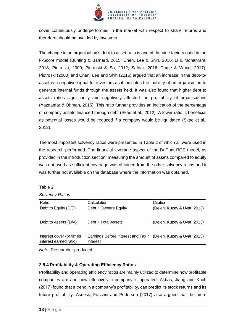
The most important solvency ratios were presented in Table 2 of which all were used in
the research performed. The financial leverage aspect of the DuPont ROE model, as
provided in the introduction section, measuring the amount of assets compared to equity
was not used as sufficient coverage was obtained from the other solvency ratios and it
was further not available on the database where the information was obtained.
Table 2 Solvency Ratios
Solvency Ratios
Note. Researcher produced.
2.5.4 Profitability & Operating Efficiency Ratios
Profitability and operating efficiency ratios are mainly utilized to determine how profitable
companies are and how effectively a company is operated. Akbas, Jiang and Koch
(2017) found that a trend in a company’s profitability, can predict its stock returns and its
future profitability. Asness, Frazzini and Pedersen (2017) also argued that the more
Ratio Calculation Citation
Debt to Equity (D/E) Debt ÷ Owners Equity (Delen, Kuzey & Uyar, 2013)
Debt to Assets (D/A) Debt ÷ Total Assets (Delen, Kuzey & Uyar, 2013)
Interest cover (or times
interest earned ratio)
Earnings Before Interest and Tax ÷
Interest
(Delen, Kuzey & Uyar, 2013)
19 | P a g e
profitable a company is, keeping all else equal, the higher the stock price should be.
Investors would therefore focus on a company’s profitability in order to evaluate future
stock price expectations. Five of the nine factors used in the F-Score model measure
profitability and operating efficiency which demonstrates the importance of this category
when performing financial ratio or fundamental analysis (Piotroski, 2000). Profitability
and operating efficiency can be measured using various financial ratio formats including
the return on assets (ROA), equity (ROE) and various profit stages in the income
statement which is compared to sales to forms the respective profit margin (Asness,
Frazzini & Pedersen, 2017; Delen, Kuzey & Uyar, 2013; Light, Maslov & Rytchkov,
2017).
From the DuPont analysis discussed in the financial ratio introduction, the importance of
the ROE and ROA as financial health evaluation metrics is clear and therefore these
ratios were further discussed below. When referring to the ROE ratio and its importance
on an individual basis, Hou, Xue, and Zhang (2015) used ROE as part of their four-factor
model to measure profitability and determined that their model is comparable and, in
some cases, delivers improved results when compared to the Cahart and Fama and
French models in identifying significant anomalies in stock returns. Ramkillawan (2014)
further found a significant positive correlation between the ROE and the average stock
returns of the Top 40 index of the Johannesburg Stock Exchange.
When referring to the ROA ratio and its importance on an individual basis, two of the five
profitability and operating efficiency ratios used in the Piotroski (2000) model were return
on assets and change in return on assets. These were selected as it provided information
about a company’s ability to generate funds internally. It has been determined by
numerous research that when applying the F-Score model to evaluate portfolios of
stocks, that significant excess returns could be realised (Bunting & Barnard, 2015; Chen,
Lee & Shih, 2016; Li & Mohanram, 2018; Piotroski, 2000; Piotroski & So, 2012; Safdar,
2016; Turtle & Wang, 2017). The G-Score model developed in Mohanram (2005) and
further used in Li and Mohanram (2018) also used the ROA in two of the eight G-Score
factors. This inclusion stems from its importance in the use of the DuPont ROA analysis
(Mohanram, 2005). It has been determined that when this model is applied to low book-
to-market stocks, that significant excess returns could be realised (Mohanram, 2005).
On a combined ROE and ROA basis, Light, Maslov and Rytchkov (2017) used ROE and
ROA as their two sole measures of profitability. They however only found ROA to deliver
significant excess stock returns. Mohanram, Saiy and Vyas (2018) also indicated that

20 | P a g e
ROE and ROA were used extensively in the banking industry to evaluate the profitability
of banks and therefore both these ratios were included as their sole profitability measures
in their B-Score model. Mohanram, Saiy and Vyas (2018) however stated that the ROE
is the main key performance ratio in the banking industry as it was widely used by
investors and bank managers.
Lee (2014) further established the importance of the Return on Capital Employed
(ROCE), as derived from Greenblatt’s investment book, which only used a two-factor
formula, comprising of the ROCE and the earnings yield (inverse of P/E ratio) to evaluate
companies. This formula was applied to over 50 years of U.S. data and the companies
who met the criteria showed significant excess returns above their peers (Lee, 2014).
Muller and Ward (2013) also found the ROCE to deliver significant excess returns when
this ratio was used to construct investment portfolios on the JSE.
From further analysis of the Piotroski (2000) model, where five of the nine factors
measured the profitability and operating efficiency ratios, one was the change in gross
profit margin. Asness, Frazzini and Pedersen (2017), also used gross profit margin
combined with ROE and ROA as part of their profitability measures and found that higher
quality firms, which have higher profitability, deliver increased share prices. In the
Bunting and Barnard (2015) research performed, the gross profit margin ratios, as used
in the Piotroski (2000) F-Score model, was not reported on the database used and
therefore the researchers used the change in the operating profit margin. This approach
appears to have been appropriate as Ball, Gerakos, Linnainmaa and Nikolaev (2015)
argued that the most appropriate measure of organisational profitability is the operating
profit. In this research, the researcher experienced the same issue with the gross profit
margin not being available, with only the operating profit margin and the net profit margin
being reported on the Iress Expert database used.
When referring to the components of the DuPont analysis, as discussed in the financial
ratio introduction, the net profit margin is used as the profitability measure (Chang,
Chichernea, & HassabElnaby, 2014; Goodman, Neamtiu, & Zhang, 2018; Mohanram,
2005; Skae et al., 2012). Various financial ratio users will therefore use the net profit
margin in analysing the financial profitability of an organisation. The researcher therefore
included both the operating profit margin and the net profit margin analysis in the
research performed. The use of both ratios for profitability analysis is further consistent
with Hsu (2014). A summary of the most important profitability and operating efficiency
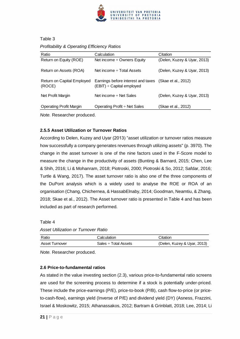
ratios were illustrated in Table 3 of which all were used in the research performed:
21 | P a g e
Table 3 Profitability & Operating Efficiency Ratios
Profitability & Operating Efficiency Ratios
Note. Researcher produced.
2.5.5 Asset Utilization or Turnover Ratios
According to Delen, Kuzey and Uyar (2013) “asset utilization or turnover ratios measure
how successfully a company generates revenues through utilizing assets" (p. 3970). The
change in the asset turnover is one of the nine factors used in the F-Score model to
measure the change in the productivity of assets (Bunting & Barnard, 2015; Chen, Lee
& Shih, 2016; Li & Mohanram, 2018; Piotroski, 2000; Piotroski & So, 2012; Safdar, 2016;
Turtle & Wang, 2017). The asset turnover ratio is also one of the three components of
the DuPont analysis which is a widely used to analyse the ROE or ROA of an
organisation (Chang, Chichernea, & HassabElnaby, 2014; Goodman, Neamtiu, & Zhang,
2018; Skae et al., 2012). The Asset turnover ratio is presented in Table 4 and has been
included as part of research performed.
Table 4 Asset Utilization or Turnover Ratio
Asset Utilization or Turnover Ratio
Note. Researcher produced.
2.6 Price-to-fundamental ratios
As stated in the value investing section (2.3), various price-to-fundamental ratio screens
are used for the screening process to determine if a stock is potentially under-priced.
These include the price-earnings (P/E), price-to-book (P/B), cash flow-to-price (or price-
to-cash-flow), earnings yield (Inverse of P/E) and dividend yield (DY) (Asness, Frazzini,
Israel & Moskowitz, 2015; Athanassakos, 2012; Bartram & Grinblatt, 2018; Lee, 2014; Li
Ratio Calculation Citation
Return on Equity (ROE) Net income ÷ Owners Equity (Delen, Kuzey & Uyar, 2013)
Return on Assets (ROA) Net income ÷ Total Assets (Delen, Kuzey & Uyar, 2013)
Return on Capital Employed
(ROCE)
Earnings before interest and taxes
(EBIT) ÷ Capital employed
(Skae et al., 2012)
Net Profit Margin Net income ÷ Net Sales (Delen, Kuzey & Uyar, 2013)
Operating Profit Margin Operating Profit ÷ Net Sales (Skae et al., 2012)
Ratio Calculation Citation
Asset Turnover Sales ÷ Total Assets (Delen, Kuzey & Uyar, 2013)

22 | P a g e
& Mohanram, 2018; Muller & Ward, 2013). The calculations of these ratios are provided
in Table 5:
Table 5 Price-to-fundamental ratios
Price-to-fundamental ratios
Note. Researcher produced. p.s. = per share.
Price-to-fundamental ratios provide an indication of investor sentiment towards a
company and its prospects (Penman & Reggiani, 2018; Skae et al., 2012). When
referring to the individual ratios, Chua, Delisle, Feng and Lee (2014) stated that the P/E
ratio might be the most important price-to-fundamental ratio when valuing a company.
The P/E ratio provides an indication of the market’s expectation of future earnings growth
(Penman & Reggiani, 2018). Conover, Jensen & Simpson (2016) stated that the DY is a
widely used investment metric and formed part of various investment strategies.
Damodaran (2012) argued that while applying the P/E and the P/B ratios as value
screens are useful for most investors, the DY is seen to be the most secure measure of
returns. This is as a stable dividend payment provides a reliable return for investors and
decreases the risk of overpaying for a stock (Conover, Jensen & Simpson, 2016).
The importance of the P/B or B/M ratio, has been establish by various research, including
the Piotroski (2000) F-Score and the Mohanram (2005) G-Score models which were
based on sorted P/B or B/M ratio stocks, as it is seen as a value measure (Bali, Cakici &
Fabozzi, 2013; Bartram & Grinblatt, 2018; Bunting & Barnard, 2015; Cordis, 2014; Fama
& French, 2008, 2012; Hoffman, 2012; Hou, Xue, & Zhang, 2015; Jiang & Lee, 2007;
Kim & Lee, 2014; Lee, 2014; Li & Mohanram, 2018; Maio & Santa-Clara, 2015).
The cash flow-to-price ratio (inverse of price-to-cash-flow ratio which measures the same
characteristics) is also seen as an important value measure (Asness, Frazzini, Israel and
Moskowitz, 2015; Lee, 2014; Muller & Ward, 2013). Van Heerden and Van Rensburg
(2015) found the cash flow-to-price ratio to be the most significant value driver on the
JSE when compared to the other value factors used namely, the dividend yield, the
Ratio Calculation Citation
Price-earnings (P/E) Market price p.s. ÷ Earnings p.s. (Skae et al., 2012)
Price-to-book (P/B) Market price p.s. ÷ Book value p.s. (Skae et al., 2012)
Price-to-cash-flow (P/CF) Market price p.s. ÷ Cash flow p.s. (Price-to-cash-flow ratio, n.d.)
Dividend yield (DY) Dividend p.s. ÷ Market price p.s. (Skae et al., 2012)

23 | P a g e
earnings yield (inverse of P/E), the sales-to-price ratio and the B/M ratio. They further
found that the value factors deliver significant explanatory power for stock returns on the
JSE. The cash flow from operations was also one of the nine factors used in the F-Score
model (Bunting & Barnard, 2015; Chen, Lee & Shih, 2016; Li & Mohanram, 2018;
Piotroski, 2000; Piotroski & So, 2012; Safdar, 2016; Turtle & Wang, 2017).
Peavler (2018) cautions against using price-to-fundamental ratios without taking other
factors and context into account. A stock with a low P/E ratio in a stable industry might
indicate that it is currently undervalued, but could also indicate that a company’s future
prospects are uncertain and that the stock presents increased risk (Peavler, 2018). Low
price-to-book ratios also act as a measure of risk, as companies with low P/B ratios,
especially those with a lower price than its book value, could be in trouble and therefore
could soon go out of business (Damodaran, 2012). This was corroborated by Penman
and Reggiani (2018) which stated that value stocks with low P/B and P/E ratios could
achieve high growth, but the growth could be risky.
Asness, Frazzini, Israel and Moskowitz (2015) further demonstrated the importance of
not only using individual pricing measures like the B/M to construct portfolios of stocks,
as various researchers have done, but to use all the value measures. The value
measures used were the book-to-market (Inverse of P/B), earnings-to-price (Inverse of
P/E), cash flow-to price (inverse of P/CF) and dividend yield ratios. They found that by
using all these value measures in conjunction to construct portfolios, that a 20%
decrease in volatility was achieved while still delivering similar returns when compared
to only using the B/M ratio individually. When the dividend yield was individually used as
n value measure, it delivered positive returns but performed the worst of all the value
measures discussed above as some companies did not pay dividends and rather
reinvested their earnings (Asness, Frazzini, Israel & Moskowitz, 2015). All four price
ratios discussed above were included as part of the research performed, as investors
would use these ratios in conjunction to evaluate shares for purchase.
2.7 Effect of financial ratios on share price performance
Some studies reviewed included multiple ratios from multiple categories and therefore
would have led to the duplication of these studies in multiple sections above. In order to
avoid duplication these studies were grouped in this section. The first set of studies
reviewed found that financial ratios showed no or minimal relationships, correlations or
predictability with share price performance. Gupta and Modise (2012), in applying the
price-dividend (inverse of DY) and price-earnings ratios to South African companies,

24 | P a g e
over a period of nearly 20 years, found no evidence of short-term or long-term
predictability in share price performance. Morar (2014) applied four financial ratios to the
emerging BRICS country stock exchanges over a period of 3 years in an attempt to
develop a simple model for stock selection. These ratios were the price-earnings, price-
sales, price-to-book and dividend yield ratios. Morar found that only the price-earnings
and dividend yield ratios showed some, but very weak correlations to share price
performance. Ma and Truong (2015) used multiple regression analysis and a much
broader dataset of 17 combined financial accounting and price-to-fundamental ratios,
over a period of 7 years (2006 – 2014), to determine which financial ratios influence the
share price performance of different sectors of the Swedish OMX stock exchange most.
The sectors analysed were banking, energy, investment, real estate and retail. The ratios
used in the study were the price-earnings ratio, price-earnings-growth ratio, price-to-
book ratio, price-sales ratio, dividend per share, earnings per share, revenue per share,
equity per share, dividend yield, net profit margin, EBITDA margin (Earnings before
interest, tax, depreciation and amortization), return on equity, return on assets, current
ratio, debt-to-equity ratio, equity ratio and lastly capital expenditure. Firstly, it was found
that the most significant financial ratios in the different sectors varied. According to Ma
and Truong (2015), the most significant ratios for the different sectors were as illustrated
in Table 6:
Table 6 Most significant financial ratios per sector
Most significant financial ratios per sector
Note. Produced from information in Ma and Truong (2015).
It was however discovered, that even though financial ratios influenced share price
growth, that this effect was marginal when compared to long-term macroeconomic trends
and only accounted for a small part of share price growth. Ma and Truong (2015) further
found that combined for all the sectors, high price ratios affected share price negatively,
and good liquidity ratios affected share price positively.
Sector Ratio
Banking Price-earnings, Dividend per share
Energy None
Investment Price-earnings, Return on equity, Equity ratio
Real Estate Price-to-sales, Return on equity, Net profit margin
Retail Price-earnings-growth, Price-to-sales, Dividend Yield, Earnings per share
25 | P a g e
The second set of studies reviewed found that certain financial ratios showed some or
strong relationships, correlations or predictability with share price performance. More
dated studies, including, Ang and Bekaert (2006), through using datasets from
developed countries namely, the United states, Germany and the United Kingdom,
determined that the dividend yield predicts excess share returns, but only in the short
term. Lewellen (2004), found that market returns on the New York Stock Exchange
(NYSE) could be predicted by the dividend yield ratio, during the period 1946-2000
tested. It was further found that higher earnings-to-price (inverse of P/E) and higher
book-to-market ratios predicted positive market returns during the 1963-2000 period
tested (Lewellen, 2004).
More recent research by Cordis (2014), found that the return on stocks can be
determined as a function of the combination of the ROE ratio, the B/M ratio (inverse of
P/B ratio) and the lagged B/M ratio for non-dividend paying stocks. Cordis (2014) further
found that for dividend paying stocks, the return on these stocks can be determined as
a function of the combination of the same ratios above, excluding the lagged B/M ratio,
but including the DY ratio. Vedd and Yassinski (2015) performed a regression analysis
on the Latin American industrial sector and used data from more than 700 companies,
over a 10-year period, to determine the relationship between financial ratios and share
prices. A strong correlation between the asset turnover ratio and the share prices of
companies in Brazil, Chile and Mexico was determined. An important but less significant
positive correlation was further determined between the debt to equity ratio and share
prices of Columbian companies. The ratios used in the study, which did not deliver
significant correlations to the industrial sector, were the return on equity, cash flow from
operations divided by sales, net profit margin, current ratio and lastly the total assets.
Arkan (2016) applied 12 financial ratios to 15 companies in the Kuwait financial market
from 2005 to 2014 to determine if financial ratios affect share prices. These companies
formed part of the industrial, services and investment sectors. Arkan (2016) determined
that certain financial ratios had a significant relationship with share price performance in
each of the sectors tested. The 12 ratios used in the research were grouped within the
five groups displayed in table 7.

26 | P a g e
Table 7 Financial ratios and groupings used
Financial ratios and groupings used
Note. Adapted from Arkan (2016).
For the industrial sector, Arkan (2016) found that a significant positive relationship exists
between ROE, ROA, fixed asset turnover, net profit margin, debt to equity, book value
per share and the market-to-book ratio when compared to the share prices. For the
service sector, Arkan (2016) found a significant positive relationship between ROE, ROA,
EPS, net profit margin, book value per share and the market-to-book ratios when
compared to share prices. Lastly, for the investment sector, Arkan (2016) found that a
significant positive relationship exists between ROE, ROA, EPS, current ratio, book value
per share and the market-to-book ratios when compared to share prices.
Asness, Frazzini, Israel and Moskowitz (2015) found that when the price-to-fundamental
ratio are used to sort stocks, that portfolios could be constructed which produce positive
returns. The price-to-fundamental ratios used to construct portfolios were the book-to-
market (Inverse of P/B), earnings-to-price (Inverse of P/E), cash flow-to-price (inverse of
P/CF) and dividend yield ratios. Yan and Zheng (2017) performed fundamental analysis
using data mining techniques from 1963-2013, where they applied more than 18 000
financial statements derived fundamental variables. They concluded that fundamental
variables can predict significant stock returns and were able to rank the top 100 signals.
This analysis was however only performed on companies from 19 developed countries
and no price-to-fundamental ratios were included as part of the research. Li and

27 | P a g e
Mohanram (2018) found that when the F-Score, G-Score and two other value driven
approaches are used in combination, when applied to portfolios of stocks listed between
1973 and 2012 on US stock exchanges, that this combined approach produced
exceptional positive returns. Li and Mohanram (2018) further found that even though the
Graham and Dodd 1934 stock screen approach, as mentioned in section 2.3, produced
excess returns when tested using the same data, that the combined approach used by
Li and Mohanram (2018) produced even greater excess returns.
Four South African JSE specific studies were noted, which found that certain financial
ratios showed strong relationships with share price performance. The first was Hoffman
(2012), which sought to determine if stock return anomalies existed on the JSE. A cross-
sectional regression analysis was performed on all the shares listed on the JSE in 2010
(376 companies), over a 25-year period. Hoffman (2012) found that the book-to-market
ratio (inverse of P/B), market capitalisation, momentum and to a lesser extent, yield-to-
book and net shares issued, when used as sorting mechanisms to produce portfolios of
stocks, lead to portfolios which generate abnormal stock returns.
Muller and Ward (2013) followed by seeking to determine which the best investment
styles were on the JSE. The 160 companies listed on the JSE based on market
capitalisation were analysed over a period of 27 years (1985-2011). Muller and Ward
(2013) found that certain investment styles, when used to develop portfolios of stocks
outperformed the JSE All Share Index. These portfolios were constructed using the
earning yield (an inverse of the P/E ratio), dividend yield, liquidity, return on capital, return
on equity, price to book, cash flow-to-price (inverse of price-to-cash flow), interest cover
and momentum. The shares in this study were however only broadly classified in two
industries namely industrial and resources.
The study attempted by the researcher did however not focus on providing an investment
style for share selection on the JSE as a whole, but attempted to provide a clarification
regarding which financial ratios affect share price to the greatest extent in different
sectors. These two mentioned studies further did not solely focus on financial ratios
where other aspect such as momentum were considered. Ramkillawan (2014) further
found a significant positive correlation between the return on equity and the average
stock return on the Top 40 index of the JSE. Out of the two financial ratios used namely,
ROE and dividend pay-out, the dividend pay-out ratio effect on the JSE was however
inconclusive.

28 | P a g e
Lastly was the research by Bunting and Barnard (2015), where fundamental analysis
was performed on the South African JSE, based on the Piotroski (2000) F-Score model,
ranging over an 11-year period ending June 2014. The F-Score study involved nine
accounting based financial ratios to classify companies into their relevant F-Scores,
where the companies with a score of zero displayed the poorest financial health and the
companies with a score of nine the best financial health. It was determined that
statistically significant correlations exist between the accounting based financial ratios
used and the share returns received. None of the above studies however focussed on
the different sectors on the JSE in isolation but grouped all the companies together. The
only study that took some cognisance of the industries was Muller and Ward (2013), but
only differentiated between the high level industrial and resource classifications to
determine which of these two industries delivered higher returns.
From the international studies investigated above, it was clear that the majority,
especially those from the U.S., found that financial ratios showed some or strong
relationships, correlations or predictability with share price performance. Only three of
these studies however focussed on the different sectors, where these were based on
less developed markets including Latin America and Kuwait. From the South African
studies investigated a clear consensus was however not reached as some found no or
minimal relationships, correlations or predictability of financial ratios and share price
performance, where others found the opposite. In summary, from a total JSE market
perspective, a greater majority seems to find that relationships exist between financial
ratios and share price performance. The results of a sector-based JSE analysis are
however still undetermined, but based on international research, could deliver value. The
hypotheses were therefore developed from the contrasts between these markets and
findings.
2.8 South Africa, a unique market place
According to Bunting and Barnard (2015), very few fundamental analysis studies have
been performed outside the United States (U.S.) equity markets. Bunting and Barnard
(2015) further noted that various differences exist between the United States accounting
standards, security regulations and market microstructure when compared to other
countries. The United States uses U.S. Generally Accepted Accounting Principles
(GAAP) as an accounting standard, where South Africa uses International Financial
Reporting Standards (IFRS) (Barth, Landsman, Lang & Williams, 2012; IFRS, 2016).
Barth, Landsman, Lang and Williams (2012) argued that significant differences exist
between the two different accounting standards.

29 | P a g e
Cinca, Molinero, and Larraz (2005) further determined that the countries where
companies are located impact the structures of their financial ratios. According to the
screener function on Iress (2018), available through the University of Pretoria’s library
database, in October 2018, 372 companies were listed on the JSE. When comparing
this with the New York stock exchange, where shares of around 2800 companies are
traded, the JSE is small in comparison (NYSE, n.d.). This further substantiates the
difference in structures of the equity markets as noted by Bunting and Barnard (2015).
Further to this, more recent literature by Konku, Rayhorn, and Yao (2018) argued that
most of the research on stock price behaviour has focussed on developed markets, as
data was more easily obtainable. Two of the three most recent fundamental analysis
studies reviewed by the researcher, were both performed only using companies listed
on U.S. Stock exchanges (Bartram & Grinblat, 2018; Li & Mohanram, 2018). The third
was that by Yan and Zheng (2017) where this research was performed on 19 developed
countries, where the authors noted that two other recent research groups used the same
19 developed countries. Konku, Rayhorn, and Yao (2018) argued that emerging market
economies have gained significant growth in the last two decades and therefore the
importance for investors have started to increase.
According to Financial Times (n.d.) “Emerging market is a term that investors use to
describe a developing country, in which investment would be expected to achieve higher
returns but be accompanied by greater risk” (para. 1). Konku, Rayhorn, and Yao (2018)
stated that the emerging market focus had been mainly based on larger emerging
economies including Brazil, Russia, India and China, but the focus was turning to smaller
emerging economies including South Africa due to the desire of diversification by
developed country investors and the potential for higher returns. Konku, Rayhorn, and
Yao (2018) further argued that studies on African markets were not as abundant as those
of other emerging markets.
An example of an emerging market study follows to demonstrate the differences between
emerging markets and developed markets, specifically China and the United States. Bin,
Chen, Puclik, and Su (2017), sought to use models which were developed based on U.S.
data, to determine if similar return results could be realised in the Chinese stock market,
which is classified as an emerging market. Some results were consistent with those of
the U.S. markets, where other results were specific to the Chinese stock markets. The
main reason for this appeared to be the difference in preferences by Chinese and U.S.

30 | P a g e
investors. Shares with smaller firm sizes, higher share trading turnovers and lower initial
share price levels tended to be the most extreme performers in U.S. markets, where the
same categories of stocks in the Chinese stock markets tended to not perform as well.
Bin, Chen, Puclik, and Su (2017) further found that, “US extreme performers are
significantly associated with factors of firm age, stock return volatility, sales trend and
earnings surprise, while Chinese extreme performers are significantly related to book-to-
price, sales-to-price and debt-to-price ratios” (p. 22).
Li, Zhang and Zheng (2018) further found that the seasonality of stock returns differed
between developed and emerging markets, where 21 of both developed and emerging
markets were tested, including South Africa as emerging market. The seasonality of
stock returns was found to be significant in developed markets with the opposite being
found in emerging markets. The two studies above provided valuable and important
examples of how developed markets differ in some instances when compared to
emerging markets.
Deloitte (2017) stated that when South Africa was included as part of the BRICS (Brazil,
Russia, India, China and South Africa) acronym in 2010, and was regarded as a first-tier
emerging market, that all the BRICS nations were regarded as performing well in terms
of rising and future demand. The BRICS landscape has however changed. While the
Chinese and Indian emerging economies were growing and could deliver the higher
returns as expected by emerging markets, South Africa was starting to display the bad
economic trends of Brazil. With various credit rating downgrades (BB+ in 2017), various
quarters of negative GDP growth realised in the most recent years, an unstable political
environment, public sector underperformance and reduced investor confidence, South
Africa might not deliver the high returns which are expected from emerging markets. It
therefore appears that the South African economic and equity market landscape is
unique, different and more volatile than those of developed markets and most of those
classified as emerging markets.
2.9 Industries/Sectors of the JSE
It is clear from financial literature that the most important financial ratios to consider is
industry specific (Yan and Zheng, 2017). Financial literature reviewed provided specific
evidence that financial ratio structures like those of manufacturing, retail and banking are
different due to the unique financial drivers of each sector (Delen, Kuzey & Uyar, 2013;
Mohanram, Saiy & Vyas, 2018). It was therefore important to understand which industry
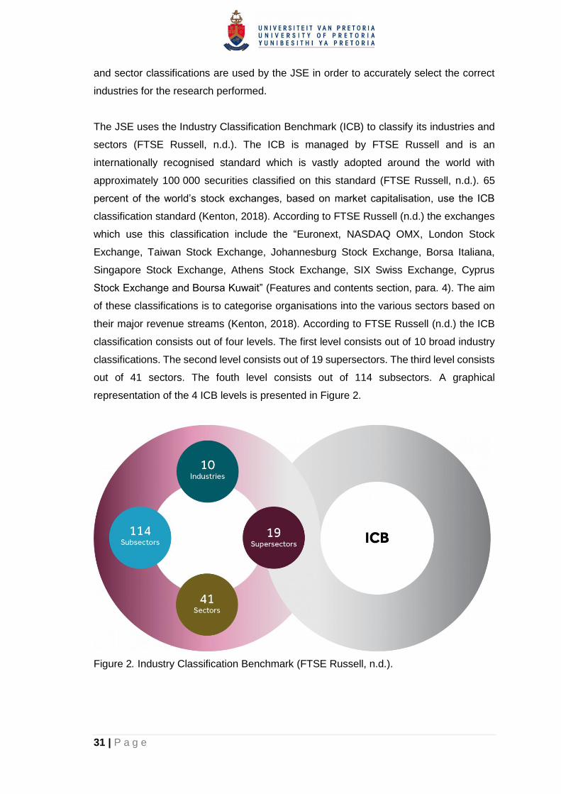
31 | P a g e
and sector classifications are used by the JSE in order to accurately select the correct
industries for the research performed.
The JSE uses the Industry Classification Benchmark (ICB) to classify its industries and
sectors (FTSE Russell, n.d.). The ICB is managed by FTSE Russell and is an
internationally recognised standard which is vastly adopted around the world with
approximately 100 000 securities classified on this standard (FTSE Russell, n.d.). 65
percent of the world’s stock exchanges, based on market capitalisation, use the ICB
classification standard (Kenton, 2018). According to FTSE Russell (n.d.) the exchanges
which use this classification include the “Euronext, NASDAQ OMX, London Stock
Exchange, Taiwan Stock Exchange, Johannesburg Stock Exchange, Borsa Italiana,
Singapore Stock Exchange, Athens Stock Exchange, SIX Swiss Exchange, Cyprus
Stock Exchange and Boursa Kuwait” (Features and contents section, para. 4). The aim
of these classifications is to categorise organisations into the various sectors based on
their major revenue streams (Kenton, 2018). According to FTSE Russell (n.d.) the ICB
classification consists out of four levels. The first level consists out of 10 broad industry
classifications. The second level consists out of 19 supersectors. The third level consists
out of 41 sectors. The fouth level consists out of 114 subsectors. A graphical
representation of the 4 ICB levels is presented in Figure 2.
Figure 2. Industry Classification Benchmark (FTSE Russell, n.d.).

32 | P a g e
2.10 Conclusion
Firstly, the most applicable investing theories and methods relating to the research
problem were discovered and reviewed, namely fundamental analysis, value investing
and growth investing. From this literature the two most important financial ratio
classification groups, namely financial accounting and price-to-fundamental ratios were
discovered and reviewed. It was found that the financial accounting ratio category
consisted mainly of liquidity, solvency, profitability, operating efficiency and asset
utilization or turnover ratios. The price-to-fundamental ratio group consisted of ratios
where the price formed one aspect of the ratio and the other aspect was related to a
financial statement fundamental.
The financial ratio theory and literature reviewed lead the researcher to select 14
financial ratios, of which 10 consisted of financial accounting ratios and 4 consisted of
price-to-fundamental ratios. Literature regarding the relationship between financial ratios
and the share price performance of companies were further reviewed and mixed results
were obtained. Most of the literature however found relationships, correlations or
predictability between some financial ratios and the share prices of companies. A clear
lack of research from a South African JSE sector perspective was however noted. These
insights assisted the researcher in forming the hypotheses.
Further, the positioning of South Africa and the Johannesburg Stock Exchange (JSE),
as an equity market among other international markets, was reviewed. It was found that
differences exist between South Africa and developed markets as South Africa was
classified as an emerging market. It was further found that most finance-based research
focussed on the larger emerging markets and that the attention was turning to smaller
emerging markets including South Africa, where research on the African continent was
not as abundant as those from other emerging markets. Various factors were starting to
affect the South African economy and markets. The higher returns as expected by well
performing emerging markets, such as China and India, might therefore not be
achievable by South Africa as it displayed unique characteristics when compared to
some other emerging markets. Lastly a review of the International Classification
Benchmark (ICB) standards, as used by the JSE for industry and sector classifications
followed, which provided an indication of the vast amount of industries and sectors
available for classification. Overall it was found that the need for this research on a JSE
sector basis was valid and that value could be achieved from both a business and
academic perspective.

33 | P a g e
CHAPTER 3 RESEARCH HYPOTHESES
Following the literature review performed in the previous Chapter, the most important
ratios identified were as indicated in Table 8:
Table 8 Financial Ratios
Financial Ratios
Note. Researcher produced. p.s. = per share.
The focus of the research was therefore to determine if any statistical relationships exist
between any of the pre-mentioned 14 ratios and the top five sectors of the JSE based
on market capitalisation. The same research hypothesis was therefore repeated five
times for each of the five sectors which were identified and discussed in Chapter 4.3.
The five hypotheses were tested using multiple linear regression statistical methods
where the methods were fully discussed in Chapter 4.8.

34 | P a g e
3.1 Hypothesis 1: Mining
Research question one (RQ1): Do statistical relationships exist between financial
ratios and share price performance of the mining sector on the JSE?
• Null hypothesis one (H01): No significant statistical relationships exist between
any financial ratios and the share price performance of the mining sector on the
JSE.
• Alternate hypothesis one (H11): Significant statistical relationships exist
between at least one or more financial ratios and the share price performance
of the mining sector on the JSE.
3.2 Hypothesis 2: Banking
Research question two (RQ2): Do statistical relationships exist between financial
ratios and share price performance of the banking sector on the JSE?
• Null hypothesis two (H02): No significant statistical relationships exist between
any financial ratios and the share price performance of the banking sector on
the JSE.
• Alternate hypothesis two (H12): Significant statistical relationships exist between
at least one or more financial ratios and the share price performance of the
banking sector on the JSE.
3.3 Hypothesis 3: Life Insurance
Research question three (RQ3): Do statistical relationships exist between financial
ratios and share price performance of the life insurance sector on the JSE?
• Null hypothesis three (H03): No significant statistical relationships exist between
any financial ratios and the share price performance of the life insurance sector
on the JSE.
• Alternate hypothesis three (H13): Significant statistical relationships exist
between at least one or more financial ratios and the share price performance
of the life insurance sector on the JSE.
3.4 Hypothesis 4: Real Estate Investment Trusts
Research question four (RQ4): Do statistical relationships exist between financial
ratios and share price performance of the real estate investment trust on the JSE?
• Null hypothesis four (H04): No significant statistical relationships exist between
any financial ratios and the share price performance of the real estate
investment trust sector on the JSE.

35 | P a g e
• Alternate hypothesis four (H14): Significant statistical relationships exist
between at least one or more financial ratios and the share price performance
of the real estate investment trust on the JSE.
3.5 Hypothesis 5: Mobile Telecommunications
Research question five (RQ5): Do statistical relationships exist between financial
ratios and share price performance of the mobile telecommunications sector on the
JSE?
• Null hypothesis five (H05): No significant statistical relationships exist between
any financial ratios and the share price performance of the mobile
telecommunications sector on the JSE.
• Alternate hypothesis five (H15): Significant statistical relationships exist between
at least one or more financial ratios and the share price performance of the
mobile telecommunications sector on the JSE.

36 | P a g e
CHAPTER 4 RESEARCH METHODOLOGY AND DESIGN
4.1 Introduction
This chapter outlines the methodology and design used to perform the testing of the
hypotheses presented in Chapter 3. Firstly, section 4.2 provides the overarching
research methodology and design used in the research. This is followed by the details
of the five populations used in the research and how they were determined on a step by
step basis in section 4.3. The unit of analysis is then defined in section 4.4, where after
section 4.5 explains that no sampling methods were used and why this was appropriate.
Section 4.6 provides information regarding the measurements used in the research and
explains why a pure measurement instrument as defined was not applicable for this
research. Further, even though validity does not fully apply to quantitative research in
the form of the reanalysis of secondary data, the validity criteria was applied and
evaluated for completeness.
Section 4.7 explained which data was obtained, from where it was obtained, how it was
prepared and cleaned for data analysis. Further the credibility and trustworthiness of the
data provider was discussed, which provided evidence regarding the reliability of the
information extracted. The details of the statistical tests performed were provided in
section 4.8, after which the research ethics considerations were discussed in section 4.9.
Lastly, the research limitations as determined before the performance of the data
analysis process was discussed in section 4.10.
4.2 Research Methodology and design
This research aimed to determine if statistically significant relationships exist between
financial ratios and the share price performance of the top five sectors on the JSE.
Positivism philosophy was adopted as highly structured methods, namely statistical
multiple linear regression analysis, was performed using accurate, uninfluenced,
secondary data, namely share prices and financial ratios in an attempt to discover law-
like generalisations (Saunders & Lewis, 2018; Saunders, Lewis & Thornhill, 2009). These
law-like generalisations were the relationships between financial ratios and share price
performance of the top five sectors of the JSE. A deductive approach, in line with that of
Bunting and Barnard (2015) and Ma and Truong (2015), was followed as the financial
ratios used in the research for testing purposes was obtained from existing financial ratio
theory and literature (Saunders & Lewis, 2018).
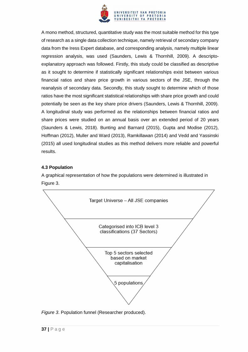
37 | P a g e
A mono method, structured, quantitative study was the most suitable method for this type
of research as a single data collection technique, namely retrieval of secondary company
data from the Iress Expert database, and corresponding analysis, namely multiple linear
regression analysis, was used (Saunders, Lewis & Thornhill, 2009). A descripto-
explanatory approach was followed. Firstly, this study could be classified as descriptive
as it sought to determine if statistically significant relationships exist between various
financial ratios and share price growth in various sectors of the JSE, through the
reanalysis of secondary data. Secondly, this study sought to determine which of those
ratios have the most significant statistical relationships with share price growth and could
potentially be seen as the key share price drivers (Saunders, Lewis & Thornhill, 2009).
A longitudinal study was performed as the relationships between financial ratios and
share prices were studied on an annual basis over an extended period of 20 years
(Saunders & Lewis, 2018). Bunting and Barnard (2015), Gupta and Modise (2012),
Hoffman (2012), Muller and Ward (2013), Ramkillawan (2014) and Vedd and Yassinski
(2015) all used longitudinal studies as this method delivers more reliable and powerful
results.
4.3 Population
A graphical representation of how the populations were determined is illustrated in
Figure 3.
Figure 3. Population funnel (Researcher produced).

38 | P a g e
The target universe was all companies as listed and delisted on the JSE. The research
performed used the third level ICB classification which includes 41 sectors to classify all
JSE companies within (FTSE Russell, n.d.). Of the 41 ICB sector classifications
available, only 37 were currently used by the JSE as companies on the JSE did not
operate in the Electricity, Gas, Water and Utilities, Oil Equipment and Services and lastly,
Aerospace and Defence sectors (Iress, 2018).
The reason for the selection of the third ICB level, was as this level of classification lead
to the most consistent industry financial drivers for the companies within to determine
the statistical relationships with financial ratios, without going in too deep when compared
to the fourth level ICB classification, or too broad when compared to the second level
ICB classification. The fourth level classifications in some subsectors contained none,
one, or very minimal companies (Iress, 2018). With 372 listed companies on the JSE in
October 2018 and 114 subsectors available on the fourth classification level, this can
easily be seen (Iress, 2018; FTSE Russell, n.d.).
The following examples are given to provide more context and substantiation on the ICB
classification levels which were used. When referring to the media sector on the third
ICB classification level, it contained five different stock codes. When that same sector
was broken up into the fourth level of the ICB classification of which publishing is one,
only one company, namely Caxton remained (Business day, 2018). Further, in another
field, when going up the classification ranks to the second level of healthcare, medical
providers such as Netcare and Life Healthcare were grouped with companies such as
Aspen and Adcock Ingram, the first being healthcare providers and the second being
medicine manufacturers (Business day, 2018). The second level ICB classification
companies mentioned operate in very different contexts with one being a health service
provider and the other a health product manufacturer. The third level was thus the most
appropriate level of classification to use.
The market capitalisation of each of the 37 ICB level three classification sectors were
selected as the benchmark due to the aspect of liquidity. According to Holden, Jacobsen
and Subrahmanyam (2014) market liquidity can be defined as “the ability to trade a
significant quantity of a security at a low cost in a short time” (p. 4). The cost and time
taken to trade securities on the JSE, are perceived to be rather consistent, but the
quantity or volume traded will depend on a few factors, of which the market capitalisation
of the organisation is highly ranked. Small market capitalisation companies will not have
39 | P a g e
as many shares available to trade on any given period when compared to large market
capitalisation firms. Further, the demand for lower market capitalisation companies are
also not always as high as for high market capitalisation companies and therefore sellers
might struggle to sell their small market capitalisation shares. High market capitalisation
firms therefore usually have higher liquidity. Muller and Ward (2013) further argued that
companies which have small market capitalisation could be too illiquid and therefore
would not be invested in by large institutional investors. Their research of the top 160
companies, out of the 350 listed on the JSE in that period, based on market capitalisation,
represented 99% of the total market capitalisation of the JSE.
The date of 28 September 2018 for the determination of market capitalisation was
selected as this was the last trading day for the month of September 2018 and the share
prices would have reflected the effects of the published financial statements for
companies with a 30 June 2018 year end. This is as time lagging was allowed for in line
with the three-month after year end JSE financial statement publication rules (JSE, n.d.).
For the market capitalisation exercise, only listed companies were selected as delisted
companies would not have any market capitalisation on 28 September 2018. To obtain
the market capitalisation of each of the ICB level three sectors, the screener function of
the Iress Expert database which is available through the University of Pretoria library
database was used with the filters as indicated in Table 9 being applied (Iress, 2018).
The reliability and credibility of the Iress Expert database was later discussed in the data
gathering process section (4.7).
Table 9 Market capitalisation filters
Market capitalisation filters
Note. Researcher produced from Iress (2018).
After applying these filters on 1 October 2018 for the date of 28 September 2018, 372
listed companies were noted which was in line with the researcher’s expectations (Iress,
2018; No of listed companies JSE, n.d.). Once the filters were applied the tools and then
compare function was selected where all the companies as filtered in Table 9 were
Filter Selection Explanation
Type Equities and Companies Only company traded equities included
Exchange JSE Securities Exchange Only those included on the JSE
Listing Status Listed Only currently listed companies included
Location South Africa The JSE is a South African stock exchange
Sectors ICB Sectors – South Africa Only To obtain market cap categorised in ICB format

40 | P a g e
selected to be compared. The edit fields option was selected where the market
capitalisation field was solely selected. The results of the applied fields were exported
into excel. The market capitalisation of each of the 37 ICB level three companies were
aggregated by way of a Pivot Table to determine the combined market capitalisation for
each sector. The top 10 Sectors based on market capitalisation as on 28 September
2018 were provided in Table 10 (Iress, 2018).
Table 10 Top 10 Market Capitalisation per ICB level 3 Sector
Top 10 Market Capitalisation per ICB level 3 Sector
Note. Researcher produced from information extracted and processed from Iress (2018).
The mining sector contained 43 companies, was deemed fit for analysis and was
therefore included as the first sector in the research performed (Iress, 2018). The
beverages and tobacco sectors only included two companies and one company
respectively. Due to the limited amount of companies included in these sectors, multiple
linear regression analysis was not fit for performing as datasets derived from single or
minimal sources could have led to distorted results. An example would be where a
company has a strong or weak leadership team or brand and even though the financial
ratios change significantly, share prices might not vary in relationship, due to the belief
and perception of the company by the investors. By having more companies in a sector
dataset with different perceptions linked to each, distortion of relationships would be
reduced. These two sectors were therefore not included in the research. The following
category was media which consisted of 5 different companies. NASPERS was however
the largest company with 99.5% of the total sector market capitalisation. The only reason
Ranking ICB level 3 sector Market Capitalisation (ZAR)
1 Mining 2 638 693 752 933
2 Beverages 2 125 028 877 529
3 Tobacco 1 640 237 579 841
4 Media 1 344 713 106 638
5 Banks 1 158 616 490 881
6 Personal Goods 605 913 080 784
7 Life Insurance 501 438 435 004
8 Real Estate Investment Trusts 476 702 628 079
9 Mobile Telecommunications 402 860 547 256
10 General Financial 399 496 702 772

41 | P a g e
this sector therefore qualified within the top sectors was due to the large market
capitalisation of NASPERS. Without NASPERS this sector would have been ranked 33rd
out of the 37 ICB level three sectors and therefore this sector was not selected for testing.
The next sector was the banking sector which included seven different banks of which
most were of comparable size and therefore were included as part of the research. The
income statements of banks were however different from most sectors as they do not
produce revenue/turnover/sales but have different income streams mainly resulting from
interest income and therefore limited profitability financial ratios were available. From
inspection of the Iress Expert database, the net profit margin, operating profit margin and
the asset turnover ratio were not available as no revenue/turnover/sales figures exist
(Iress, 2018). The other profitability ratios were still available for use and therefore this
sector was selected as the second sector to be included in the research, where the three
ratios discussed could not be tested.
The personal goods sector which followed only contained two companies, namely
Compagnie Financière Richemont and Imbalie Beauty Limited. The first made up nearly
100 % of the market capitalisation where the second was experiencing various issues
and uncertainty with multiple cautionary trading announcements being made by the JSE
during 2018 (Sharenet SENS, 2018). This sector was therefore not fit for analysis due to
mainly one company making up the whole sector and was therefore excluded from the
research. The next sector was the life insurance sector. Six companies were present in
this sector, was deemed fit for analysis and was therefore included as the third sector to
be included in the research. The last sectors were real estate investments trusts which
included 44 companies and mobile telecommunications which included four companies.
These sectors were deemed fit for analysis and therefore were included as the fourth
and fifth sectors in the research respectively.
In closing, the five ICB level three sectors namely mining, banking, life insurance, real
estate investment trusts and mobile telecommunications and all the accompanying
companies classified within these sectors were selected as the five populations to be
used in the research performed.
4.4 Unit of analysis
The units of analysis were the share prices and related defined financial ratios for the
individual listed and delisted companies in each of the five sectors, namely mining,
42 | P a g e
banks, life insurance, real estate investment trusts and mobile telecommunications of the
JSE for the 21-year period from 1 January 1997 to 30 September 2018.
4.5 Sampling method and size
No sampling methods were used during the research performed. All companies both
listed and delisted, which formed part of the five sectors indicated above, were included
for testing purposes. This information was obtained on an annual basis where financial
ratios and share price data were available from the Iress Expert database for the 21-year
period from 1 January 1997 – 30 September 2018. Seeing that this study was
longitudinal time series-based research it was appropriate to use the full data-set and
not apply any sampling methods or sampling sizes.
4.6 Measurement instrument
The study made use of quantitative secondary data, retrieved from a database named
Iress Expert, in the form of share prices and financial ratios. There therefore were no
measurement instruments as traditionally defined in research literature such as surveys,
questionnaires, interviews etc. (Saunders & Lewis, 2018). The credibility and reliability
of the information obtained from the Iress Expert database was discussed in section 4.7.
Financial ratios were reliable measurements to use in the research they are tools to
evaluate firm performance and financial health and can be applied over various sizes of
companies in the same industries, leading to a universal comparison tool (Delen, Kuzey
& Uyar, 2013; Financial ratios, n.d.; Yan & Zheng, 2017). Financial ratios are most
effective when used to track company performance over time (Financial ratios, n.d.). In
the research performed, the percentage change in share price and the accompanying
financial ratios were therefore compared from year to year and were tracked over time.
The year of 1997 was set as the base period for comparison and if no data was available
for 1997, or the company was listed in a later period, then the first subsequent period
was used as base period.
Multiple linear regression was used as the statistical testing method to determine if
financial ratios have significant statistical relationships with the share price movement of
the different industries selected. Various studies including Arkan (2016), Ma and Truong
(2015) and Morar (2014) have all used multiple linear regression analysis to determine
if statistical relationships exist between financial ratios and share prices. The reason for
not applying correlation analysis as a statistical method on an individual basis, is as
correlation analysis does not address the issue of multicollinearity, which is caused when

43 | P a g e
independent variables, namely the financial ratios used in this study, are highly
correlated with each other (Hair, Black, Babin & Anderson, 2010; Wegner, 2016).
Multicollinearity causes the independent variables to overlap when determining the
relationship with the dependent variable, namely the share price, which could lead to
unreliable results (Hair et al., 2010; Wegner, 2016). Correlation analysis further does not
consider the effects of the other variables as a combined group on the independent
variable. Therefore, more rigorous multiple linear regression hypothesis tests were used
to determine the statistical significance of the relationships between the percentage
change in share price from the previous period and financial ratios (Wegner, 2016).
Even though the validity aspects of quantitative research based on secondary data is not
always discussed as the credibility and reliability of the sources of secondary data is
normally of most importance a quick review and reasoning of the five validity factors were
performed in Table 11. Seeing that the most appropriate and reliable statistical methods,
data and data formats were used, the reliability and the validity of the results were
assured.
Table 11 Validity factors and reasoning for each
Validity factors and reasoning for each
Note. Adapted from Saunders and Lewis (2018).
Factor Reasoning
Subject selection No bias in subject selection as the selected ratios, sectors and related companies
were determined by direct literature and mathematical calculation, where the full
population was included for each sector.
History Longitudinal research performed over an extended period of 20 years is deemed
sufficient.
Testing Data collection was fully unbiased as the data was based on audited and published
financial statements. Further, all available datapoints were included for each sector
with the exceptions where data errors were incurred from the secondary data or
where significant outliers were detected which would distort the results of the multiple
linier regression per group significantly due to error or unusual circumstances.
Mortality All “subjects” were included including those listed after 1997 or which were delisted
afterwards up until 2018. The inclusion or loss of certain companies due to delisting
or liquidation strengthens the quality of the research as survivorship bias is removed
(Hoffman, 2012; Muller & Ward, 2013; Bunting & Barnard, 2015).
Ambiguity about
causal direction
Relationship variables were clearly determined by theoretical and academic literature.
Stock prices were determinants of financial ratios, financial ratios were not
determinants of stock prices except for price-to fundamental-ratios where one of the
two components of the ratios were the share price. This concern was however
resolved as part of the process of lagging the share prices by three months when
compared to the share prices used in the four price-to-fundamental ratios affected.

44 | P a g e
4.7 Data gathering process
Secondary quantitative data, namely financial ratios and share prices, for all listed and
delisted companies in the five selected sectors, were extracted from the Iress Expert
database which is available through the University of Pretoria library database. Firstly,
the fact that this database is made available by the University of Pretoria for student use
provides some initial credibility. Iress is a global and reputable supplier of financial
markets information, which has been in operation since 1993 (Iress, n.d.). Iress is also
used by the Business Day newspaper, a widely used South African newspaper, for their
daily market information (Business day, 2018). Iress further purchased INET BFA, a
consolidated company of McGregor BFA and INET Bridge, which was owned by
Media24 in September 2016 (“IRESS to buy” 2016). INET BFA was used during the
research of Bunting and Barnard (2015), Muller and Ward (2013), Herbst (2017) and was
considered as a reliable alternative source by Morar (2014). Hoffman (2012) further used
McGregor BFA before the merging with INET Bridge, of which the consolidated company
is owned by Iress.
Further, when discussing the objective of the research performed with a Gordon Institute
of Business Science library representative, it was indicated that the Iress Expert
database would be best suited platform to use for the detailed, longitudinal research to
be performed. This was as this database was the most complete, contained the longest
time period of complete data and was able to extract the data in an excel format. Overall,
the data received from the database was therefore deemed to be reliable as it was
obtained from a credible and trustworthy source.
The process explained below was performed five times for each of the five sectors
selected namely mining, banking, life insurance, real estate investment trusts and mobile
telecommunications. The Iress Expert database was accessed, and the screener
function was selected. The filters as illustrated in Table 12 were applied:

45 | P a g e
Table 12 Applied Iress Expert filters
Applied Iress Expert filters
Note. Researcher produced from Iress (2018).
Delisted shares were also selected for testing to eliminate survivorship bias. This is an
occurrence where research only considers companies which are still listed, operating
and have survived through different cycles, while ignoring the companies which did not
survive and were delisted due to bad performance, as an example, which leads to
unreliable results. Bunting and Barnard (2015), Hoffman (2012), Muller and Ward (2013)
also incorporated delisted companies in their research in order to eliminate survivorship
bias. The Iress Expert database keeps all the data for the delisted companies. Another
risk documented by Bunting and Barnard (2015) was the backfill bias risk, where
company data is included before they are listed on a stock exchange, in this instance the
JSE. The Iress Expert database did not include company data before listing and only
reported ratios based on publicly announced JSE results. The backfill bias risk was
therefore mitigated.
Based on the literature review performed, the various classifications of financial ratios
available, and the results achieved by previous studies evaluated in section 2.5 and 2.6,
the financial ratios as illustrated in Table 13 were selected in the edit fields section and
were included in the research.
Filter Selection Explanation
Type Equities and Companies Only company traded equities included
Exchange JSE Securities Exchange Only those included on the JSE
Listing Status Listed & Delisted Listed and delisted companies included
Location South Africa The JSE is a South African stock exchange
Sectors ICB Sectors – South Africa Only - "Individual sector" The 5 ICB sectors were selected individually

46 | P a g e
Table 13 Financial ratios selected
Financial ratios selected
Note. Researcher produced. p.s. = per share.
Further to the above ratios selected, the closing share price was also selected as part of
the edit field option. According to the study performed by Morar (2014), the limitations
discussed therein, and the review of other studies performed, a minimum of 10 years
was evident for such a study to be performed (Bartram & Grinblat, 2018; Bunting &
Barnard, 2015; Gupta & Modise, 2012; Hoffman, 2012; Li & Mohanram, 2018; Muller &
Ward, 2013; Vedd & Yassinki, 2015). A 20-year period was selected from 1 January
1997 to 30 September 2018 on the database, with the year 1997 being set as the base
year. A longer period might have caused issues, as through inspection, it was noticed
that older datasets tended to be rather incomplete. The period until 30 September 2018
was selected as various organisations have 28 February as well as 30 June year ends,
and therefore their 20-year comparison period would only be fulfilled on 28 February
2018 or 30 June 2018 respectively.

47 | P a g e
According to the JSE, all JSE listed companies have three months after their financial
year ends to publish their results on SENS (JSE, n.d.). Share prices of listed companies
would therefore not immediately be affected by financial information on the date of a
reporting period. The share data as obtained from Iress Expert was therefore time lagged
for a period of three months after the financial reporting period and therefore the date of
30 September 2018 was selected so that the companies with a financial year end of 30
June 2018 were still included as part of the research. This approach was line with those
taken by Muller and Ward (2013) and Bunting and Barnard (2015) in their research
performed. The periods as stipulated above were selected on the Iress Expert database
by inputting the dates on the custom period selector and requesting these ratios to be
reported monthly to ensure that any companies with unusual year ends were reflected.
After the selection of the dates the data was exported to excel.
In the research performed by Muller and Ward (2013), name changes were tracked to
ensure that companies that went through name changes were not seen as different
entities. From inspection of the excel data extracted from the Iress Expert Database, it
was confirmed that companies who underwent name changes were retrospectively
updated with the new names. This was in line with the findings of Bunting and Barnard
(2015) while using the INET database. An example for illustration purposes, in the Mining
sector, was Sentula Mining Limited which undertook a name change to Unicorn Capital
Partners Limited on the 2nd of August 2017 (Sentula Mining Limited, 2017). The
researcher previously audited this company and therefore was fully aware of the name
change and therefore investigated. From inspection of the data extracted the name
Unicorn Capital Partners reflected since 1997/01/31, the first day data this company was
extracted for the mining sector.
Data cleaning was thereafter performed in excel, by removing the datapoints where all
the financial data for a specific period, for a company, was not present. These removed
datapoints were kept on a separate spreadsheet so that they can be accessed at a later
stage. This method was in line with that performed by Muller and Ward (2013). This was
performed throughout the datasets except where the dividend yield ratio was the only
ratio where a zero value was displayed. This was as companies might not pay dividends
every single year and therefore the ratio would be expected to be zero and not an error
or missing variable. Instances were also noted where the dividend yield was blank with
no value where all the other 13 ratios displayed values. If all the preceding and following
years displayed a zero-dividend yield ratio this blank ratio was also changed to zero.

48 | P a g e
Where the dividend yield ratio consistently displayed a value for the preceding and
following years, but was blank on one line of the dataset, the individual data line was
removed and was deemed as incomplete. The reason for this action is due to the fact
that companies have dividend policies in place. If the company never pays dividends as
in the first instance, then it would be safe to determine that no sudden dividends would
be paid where the blanks were displayed. If a company displays a usual trend of paying
dividends, then it normally happens that consistent dividends are paid based on a
predetermined calculation for example 5% of profit etc.
Where companies which were previously listed were unlisted in subsequent years, the
data of those companies were only included up until the latest published financial ratios
and the three-month lagged share price before the company was delisted. The three
month lagged share prices were then copied and inserted next to the financial ratios
applicable. For example, if a company had a financial year end of 30 June, the three
month later lagged 30 September share price was copied and inserted next to the 30
June financial ratios. The percentage change in the share price from the previous year
was then calculated to produce a new variable which would replace the actual share
price for the applicable year. This was achieved by applying Equation 2 to each of the
three months lagged share prices for the relevant years.
Equation 2. Percentage change equation
Source: Adapted from Percentage change (n.d.).
The initial base period (Pt-1) was set as 1997 and the next period (Pt) as 1998. Every
year these periods would move in line with the accompanying financial ratio periods.
When companies were only listed in a later period, the listing year was set as (Pt-1) and
the next as (Pt). It is important to understand that the financial year end dates for some
companies in the various industries differed, as the financial year end date of a company
can be chosen and also in some instances, companies undertook financial year end
changes during the course of their operations which is normal and expected. Seeing that
all the share price data in the different periods were able to be standardised into a
consistent universal measure, namely percentage change from previous period,

49 | P a g e
companies with different market capitalisation and especially higher and lower share
prices were able to be compared to each other and be included in the same dataset.
Lastly with this one consistent measure of percentage change in share price, weight was
equally distributed between each datapoint, even if the share price was minimal or
substantial, causing no company to carry more weight than another. Please note all data
cleaning processes described above were performed in Microsoft Excel 2017 before
performing the data analysis in IBM SPSS v25.
4.8 Data analysis approach
The data analysis approach used for testing hypothesis 1-5 was a stepwise multiple
linear regression analysis approach. This approach is a widely used tool in business and
specifically finance when working with returns (Wegner, 2016). This method aims to
determine the relationship between multiple independent variables and a dependent
variable and was therefore best fit for the research that was performed (Hair et al., 2010;
Wegner, 2016). The percentage change in share prices from period to period was
classified as the dependent variable (y). Each of the 14 financial ratios were classified
as the independent variable (x).
The stepwise regression was performed using the automated stepwise regression
function in IBM SPSS v25 (George & Mallery, 2019). The stepwise regression is the most
popular and commonly used regression model, specifically in IBM SPSS v25, as it
combines both forward and backward regression procedures and takes the effect of all
variables entered into account to find the model, from multiple combinations, with the
most explanatory power (George & Mallery, 2019; Hair et al., 2010). Firstly, the
independent variable which delivers the greatest contribution is added, after which the
remaining variables are then included based on their contribution in addition to the
variables already included (Hair et al., 2010). Arkan (2016) and Ma and Truong (2015)
also used a stepwise regression model to determine which financial ratios had the most
significant relationship with share price performance for the selected sectors.
All the variables and accompanying data used in the population first needed to fulfil the
multiple linear regression assumptions before the automated stepwise regression could
be performed as defined below (Bezuidenhout, 2017; Laerd Statistics, n.d.-a; Parke,
2013). Only after the all assumptions were met using a normal regression model for the
testing of assumptions was the automatic stepwise regression performed. The reason
for performing the assumption testing using normal regression testing in IBM SPSS v25
was to provide all variables initially entered an equal chance, after being corrected for

50 | P a g e
outliers, highly influential points, highly leveraged points, multicollinearity etc., to possibly
form part of the stepwise regression results. The approach of first ensuring the
assumptions were met before applying stepwise regression was similar to that used by
Ma and Truong (2015). For all testing performed the level of significance was set at 0.05
which leads to a 95% confidence interval.
Multiple Linear Regression Assumptions
The first assumption is that one continuously measurable dependent variable is used.
Secondly, two or more independent variables are used. The observations (residuals) are
then independent, which is followed by ensuring that the dependent variable (percentage
change in share price) has a linear relationship with the independent variables (financial
ratios). The data then needs to be homoscedastic. It should then be ensured that there
is no multicollinearity and that no significant outliers, highly influential of highly leveraged
points exist. Lastly, the residuals should be approximately normally distributed
(Bezuidenhout, 2017; Laerd Statistics, n.d.-a; Parke, 2013).
4.8.1 Assumption 1
One dependent variable is used which is measured on a continuous scale.
The annual percentage change in the share price is the dependent variable and it is
measured on a continuous scale.
4.8.2 Assumption 2
Two or more independent variables are used.
There are 14 independent variables, namely the financial ratios, which were measured
on a continuous level as indicated in Table 14. The only sector where all 14 independent
variables could not be applied but only 11 was the banking sector as the banking sector
could not produce the net profit margin, operating profit margin or total asset turnover
due to the format of its operations and financial statements. The banking sector does not
contain revenue/turnover/sales as it mainly obtains funds through the income obtained
from loan income. All the 11 other ratios were however consistently applied during the
testing of the banking sector.

51 | P a g e
Table 14 Financial ratios selected
Financial ratios selected
Note. Researcher produced. p.s. = per share.
4.8.3 Assumption 3
The observations (residuals) are independent.
According to Weiers, Gray & Peters (2011), time series-based regression models, such
as which was performed by the researcher are especially susceptible to autocorrelation,
which is the phenomenon which occurs when independence of observations does not
exist. The most suitable way to test for the independence of observations is by using the
Durbin-Watson test (Durbin & Watson, 1950, 1951; Laerd Statistics, n.d.-a; Parke, 2013;
Weiers et al., 2011). Independence of observations was tested by calculating the Durbin
Watson Statistic using IBM SPSS v25. Any scores close to 2 were accepted as this
indicated that there was independence of observations (Bezuidenhout, 2017;
Nightingale, 2018; The Open University, n.d.; Weiers et al., 2011).
52 | P a g e
4.8.4 Assumption 4
The dependent variable (percentage change in share price) has a linear relationship with
the independent variables (financial ratios).
The first step to substantiate this assumption was to produce scatter plots to determine
the degree of linearity between the dependent variable (y) and each independent
variable (x) (Hair et al., 2010; Wegner, 2016; Laerd Statistics, n.d.-a; Parke, 2013; The
Open University, n.d.). Scatterplots were produced in IBM SPSS v25 between the
percentage change in share price (dependent variable) and each financial ratio
(independent variable). The percentage change in the share price was placed on the y-
axis and the relevant financial ratio on the x-axis. These were inspected to determine if
linear relationships existed between the variables, the direction, namely positive or
negative and the strength of the relationships between the variables were inspected and
the need for removal of any additional outliers were considered. Professional judgement
as a financial expert was applied when removing any outliers which would significantly
distort the results and lead to decreased linear fit. Outliers were classified as those
datapoints which significantly would affect the linear function of the multiple linear
regression analysis for the specific sector and was not representative of the majority of
the sectors results or occurred due to special circumstances. Any outliers were kept in a
separate sheet which was in line with Muller and Ward (2013).
After the production of scatterplots, partial regression plots were produced and inspected
for linearity in SPSS with the percentage change in share price being placed on the y-
axis and the respective financial ratio being placed on the x-axis (Bezuidenhout, 2017;
Hair et al., 2010; Laerd Statistics, n.d.-a). Further, the scatterplot of standardized residual
values versus the standardized predicted values was inspected and a Loess curve was
added to this graph to ensure that the residuals were roughly scattered around zero to
ensure the relationships were linear (UCLA Institute for Digital Research and Education,
n.d.). Some of the ratios selected did not present strong linear relationships, where
others displayed a stronger relationship with the data presented. Seeing that an
automated stepwise regression model was used the stepwise model would have
removed the independent variables which did not have a strong linear relationship with
the percentage change in share price and only keep the significant independent variables
which displayed a strong linear relationship for each sector.
4.8.5 Assumption 5
The data is homoscedastic.

53 | P a g e
Homoscedasticity was ensured by inspecting the scatterplot of the regression
standardised residual versus the regression standardized predicted value (Parke, 2013;
The Open University, n.d.). Even though the inspection of this scatterplot provides some
comfort, it does not provide statistical significance tests where the homoscedasticity is
determined by a way of a hypothesis test. The researcher therefore opted to perform
more rigorous homoscedasticity hypothesis tests.
The Breusch-Pagan and the Koenker tests were available (Breusch & Pagan, 1979;
Koenker, 1981). The Koenker was an improved and more reliable test as it corrected an
estimation error which was present in the Breusch-Pagan test (Koenker, 1981). Another
test namely White’s test (White, 1980) for homoscedasticity was also available, but it
was deemed that the Koenker test had more power than that of White’s test (Lyon &
Tsai, 1996). The Koenker test was therefore selected for use in the research as it was
deemed to be the most effective homoscedasticity tests out of the three mentioned.
A macro, which was developed by Daryanto (2018), was obtained which could be ran on
SPSS to perform this test automatically. Even though this macro produced both the
Breusch-Pagan and Koenker Results, only the Koenker results were focussed on and
used in this research as it was more reliable as explained above. If data is not
homoscedastic then it is classified as being heteroscedastic. The null hypothesis per the
test was that heteroskedasticity was not present (homoscedastic). If a significance value
of less than 0.05 was obtained, then the null hypothesis would be rejected indicating that
the data was heteroscedastic and is in violation of the assumption of homoscedasticity.
According to Hair et al. (2010) if heteroscedasticity was detected, the data could be
transformed using similar techniques to those used in transformations to achieve
normality, for example by applying a square root or inverse transformation, depending
on the nature on the heteroscedasticity.
4.8.6 Assumption 6
Multicollinearity is not present.
Multicollinearity is the phenomenon which occurs when an independent variable’s effect
can be largely predicted by another independent variable (Hair et al., 2010; Laerd
Statistics, n.d.-a). The inspection of a correlation analysis is a simple way of determining
if multicollinearity exists (Hair et al., 2010; Wegner, 2016; Weiers et al., 2011). This is
however not the best method as it does not consider the effect of the other financial
variables when calculated (Hair et al., 2010).

54 | P a g e
The Variance Inflation Factor (VIF) and tolerance values are much more reliable methods
of testing for multicollinearity and therefore the values of these tests were inspected in
IBM SPSS v25 (Bezuidenhout, 2017; Hair et al., 2010; Herbst, 2017; Laerd Statistics,
n.d.-a; Ma & Truong, 2015; Nightingale, 2018; Parke, 2013; The Open University, n.d.).
Any VIF score below 10, or tolerance factor of more than 0.1 was accepted
(Bezuidenhout, 2017; Herbst, 2017; Ma & Truong, 2015; Nightingale, 2018; Parke, 2013;
The Open University, n.d.). If higher scores were obtained, then the variables with the
highest scores were removed and the tests were rerun until all VIF scores were below
10 and all tolerance levels were above 0.1. These tests were performed firstly with all
the variables in place and only after all variables displayed acceptable VIF and tolerance
values was the stepwise regression run.
4.8.7 Assumption 7
No significant outliers, highly influential or highly leveraged points exist.
Significant outliers were first removed as stated earlier in Assumption 4 by way of the
inspection of scatterplots and residual plots. After this process, casewise diagnostics
were performed using IBM SPSS v25 by setting the value to detect outliers with values
more than positive or negative three standard deviations (Bezuidenhout, 2017; Laerd
Statistics, n.d.-a; La Trobe University, n.d.; Parke, 2013). Any outliers which were
detected by the casewise diagnostics were removed from the dataset which after the
regression was reperformed until no further outliers existed.
Highly influential points were firstly evaluated by inspecting the Cook’s distance values
(Parke, 2013; Laerd Statistics, n.d.-a) Any datapoints with Cook’s distance values of
more than one was seen as highly influential and were removed (Bezuidenhout, 2017;
The Open University, n.d.). Further to this, a scatterplot plotting Cook’s distance value
(y-axis) by centred leverage value (x-axis) was produced and inspected to further detect
any highly influential or leveraged points (IBM Corporation, n.d.). Some datapoints might
possess larger Cook’s distance values when compared to other datapoints, which will
add increased variability to the regression estimates, but if these values do not possess
a high leverage value then it is not likely to affect the regression equation (IBM
Corporation, n.d.). Similarly, some datapoints might possess a higher leverage value
when compared to other datapoints, but if it does not possess a large Cook’s distance
then it is not likely to exert undue influence on the regression model (IBM Corporation,
n.d.). The values of each of the scores on the scatterplot in combination were therefore

55 | P a g e
analysed to determine if any highly leveraged and influential points existed, and if so,
these were removed (IBM Corporation, n.d.).
4.8.8 Assumption 8
The residuals are approximately normally distributed.
Firstly, the histogram of regression standardized residuals was inspected in IBM SPSS
v25, as this is the simplest visual inspection method (Hair et al., 2010; Laerd Statistics,
n.d.-a; Parke, 2013). Secondly, the normal P-P plot of regression standardized residuals
was inspected (Bezuidenhout, 2017; Hair et al., 2010; Laerd Statistics, n.d.-a; The Open
University, n.d., UCLA Institute for Digital Research and Education, n.d.). Hair et al.
(2010) argued that this method is beneficial as the inspection of the histogram of
residuals, in instances where small samples exist, could lead to a badly-formed
distribution which is difficult to interpret. Residual plots which followed close to the
diagonal line provided evidence that the residuals were approximately normally
distributed (Hair et al., 2010).
According to Hair et al. (2010) the inspection of graphical presentations is not to replace
other tools available, but these methods should be used in conjunction with other
methods including the evaluation of skewness and kurtosis values. To obtain additional
comfort regarding the normality of residuals using skewness and kurtosis, general rules
of thumbs are available which were evaluated against the skewness and kurtosis values
delivered by the standardized residuals. A skewness value of above ± 1 indicates that a
distribution is heavily skewed (George & Mallery, 2019; GoodData Corporation, n.d.; Hair
et al., 2010). A skewness value between ±1 and ± 0.5 in the same direction indicates a
moderately skewed distribution (GoodData Corporation, n.d.). A skewness value of
between ± 0.5 and 0 indicates that the distribution is approximately normally distributed
and symmetric (GoodData Corporation, n.d.). When referring to the kurtosis rule of
thumb, the same values are applicable to substantiate the normality aspect relating to
skewness (George & Mallery, 2019). Both the skewness and kurtosis values of the
residuals were inspected to ensure that these values were between ± 0.5 each to obtain
comfort that the residuals were approximately normally distributed.
Further, to obtain additional comfort regarding the normality of residuals, more rigorous
testing was performed. SPSS can produce two types of normality tests for residuals
namely the Shapiro-Wilk and the Kolmogorov-Smirnov test and these were also the most
commonly used tests (Hair et al., 2010; Laerd Statistics, n.d.-b). According to Ghasemi

56 | P a g e
and Zahediasl (2012), the Kolmogorov-Smirnov test has lower power when compared to
the Shapiro-Wilk test and therefore the second test should rather be used in combination
with the inspection of visual graphs in SPSS to obtain the best results. The Shapiro-Wilk
test, similar to that used by Nightingale (2018), was therefore used in the research
performed.
Hair et al. (2010) however warns that the statistical normality tests discussed above,
namely the Shapiro-Wilk and the Kolmogorov-Smirnov tests, are less useful in small
samples (<30) and could be oversensitive in large samples (>1000) and therefore should
be combined with the inspection of visual plots to ensure approximate normal
distribution. Kim (2013) seems to take a more conservative approach with regard to large
samples and indicates that both these tests are more useful for samples smaller than
300 and may be unreliable for larger samples. The results of the Shapiro-Wilk test on a
standalone basis might therefore not deliver an actual representation of normality for all
the sectors tested due to the large variation in sample sizes between the sectors tested.
To perform the Shapiro-Wilk test, the standardized and unstandardized residuals were
inserted in the explore function of the descriptive statistics selection in SPSS. Normality
plots with tests were then selected. The significance of the Shapiro-Wilk test was first
inspected, and it was ensured that for both standardized and unstandardized residuals
the significance was consistent. The value of significance was then inspected and if
these values were larger than 0.05 it could provide evidence that the errors were
normally distributed (Laerd Statistics, n.d.-b). Lastly, after this test was executed the box
plot and normal Q-Q plot of standardized residuals was inspected (Laerd Statistics, n.d.-
a; Laerd Statistics, n.d.-b; Parke, 2013; UCLA Institute for Digital Research and
Education, n.d.). The box plot inspection was combined with that of the extreme values
(outlier) output to identify any datapoints which were both extreme outliers and presented
extreme outlying residuals which affected the normality of residuals.
According to Parke (2013), if certain variables appear to lead to non-normality, an option
is to remove these individual variables. The most significant of the overlapping datapoints
which were both extreme outliers and non-normally distributed were therefore removed.
The researcher used careful consideration when analysing the results of the Shapiro-
Wilk test in combination with the graphical representations and the skewness and
kurtosis values to make an informed decision regarding the approximate normal
distribution of residuals of each of the five sectors.

57 | P a g e
Finalization
It is of importance to note that the aim of this study was not to develop a model for
prediction purposes where every single possible financial ratio was included, but only to
determine which financial ratios from those selected based on the literature reviews
performed have the strongest statistical relationship to share price performance. After all
of the eight assumptions above were satisfied, the automatic stepwise regression was
performed in IBM SPSS v25 and the most significant financial ratios for each sector was
identified based on the most commonly used 0.05 level of significance, which leads to a
95% confidence interval (Wegner, 2016). Seeing that an automatic stepwise regression
was used, the combination of the statistically significant financial ratios together delivered
the highest R2 value possible with all the variables available.
4.9 Research Ethics
This research used secondary data, in the form of financial ratio and share price
information, which were publicly available data, seeing that this information pertained to
publicly listed companies on the JSE. The database used, namely Iress Expert, was
made available for all students via the University of Pretoria library database and
therefore no specific approval had to be obtained to use this data from Iress, the supplier.
No human data was gathered during this research and therefore no further ethical
concerns arose from this aspect.
4.10 Research Limitations
The preliminary limitations as determined before the statistical testing of the data
obtained follows. The study firstly was performed on the top five JSE sectors based on
market capitalisation even though 37 of the total 41 ICB level three sectors were
available on the JSE for analysis (FTSE Russell, n.d.; Iress, 2018). Due to time
constraints, more sectors were not able to be investigated, but in addition to the time
constraints, some of the sectors would have not been fit for multiple linear regression
analysis as some would only contain one or very minimal companies within the sectors.
This was clearly noted from section 4.3 where the initial population was determined,
where some of the high market capitalisation ICB level three sectors like tobacco only
included one company, which would have led to insufficient datapoints for effectively
performing multiple linear regression analysis. This was therefore a limitation to the
study.
Secondly, the database used to obtain the secondary data, namely share prices and
financial ratios, could only provide these on an annual basis. Even though financial ratios

58 | P a g e
in South Africa are mostly generally calculated on an annual basis, as JSE listed
companies are only required to be audited on an annual basis, based on their year-end
financial results, the JSE requires listed companies to release results two times a year,
namely at an interim period and at a final year end period (JSE, n.d.). Seeing that interim
ratios were not available, which would have led to more datapoints for testing purposes,
this was seen as a limitation.
Thirdly, share prices were lagged for three months to ensure that financial statement
information would have been released to investors in line with JSE regulations (JSE,
n.d.). Companies might however release their results on earlier periods than exactly
three months from financial yearend or investors might not all respond to financial
information on precisely the day the financial information is released. This is therefore a
limitation but was the most appropriate method to perform the research as a similar
method was used by Bunting and Barnard (2015) and Muller and Ward (2013).
Lastly, some of the research performed by others, especially those of Muller and Ward
(2013) add dividends received together with the change in the share price, in order to
calculate the annual returns percentage in the period. In this research the focus is
however not on returns but only the pure change in the share price. Some might label
this as a limitation even though our research includes the dividend yield ratio which would
be compared to the change in share price. Nonetheless this was classified as a limitation.
59 | P a g e
CHAPTER 5 RESULTS
5.1 Introduction
This chapter presents the results of the tests performed in order to either accept or reject
the null hypothesis of each of the five-hypotheses documented in Chapter 3. Firstly, the
relevant hypothesis was restated under each section. This was followed by a description
of the sample obtained and the cleaning of the data for multiple linear regression
assumption purposes. The main findings of the eight multiple linear regression analysis
findings were then stated. Further the descriptive statistics of the multiple linear
regression were displayed. Lastly, the final stepwise regression results were presented
after which the section was completed by presenting the results of the rejection, or
acceptance of the null hypothesis.
The IBM SPSS v25 and other outputs of the eight multiple linear regression assumptions,
which first needed to be fulfilled as described in Chapter 4.8, were included under
Appendix B, under the first section of the relevant Hypothesis. The IBM SPSS v25
outputs of the stepwise multiple linear regression were included in Appendix B, under
the second section of the relevant hypothesis.
5.2 Hypothesis 1: Mining
Research question two (RQ1): Do statistical relationships exist between financial
ratios and share price performance of the mining sector on the JSE?
• Null hypothesis two (H01): No significant statistical relationships exist between
any financial ratios and the share price performance of the mining sector on the
JSE.
• Alternate hypothesis two (H11): Significant statistical relationships exist between
at least one or more financial ratios and the share price performance of the mining
sector on the JSE.
5.2.1 Description of data obtained and cleaned
The full dataset from 1 January 1997 to 30 September 2018 for the ICB level 3 mining
sector was obtained and cleaned for multiple linear regression purposes as displayed
in Table 15.
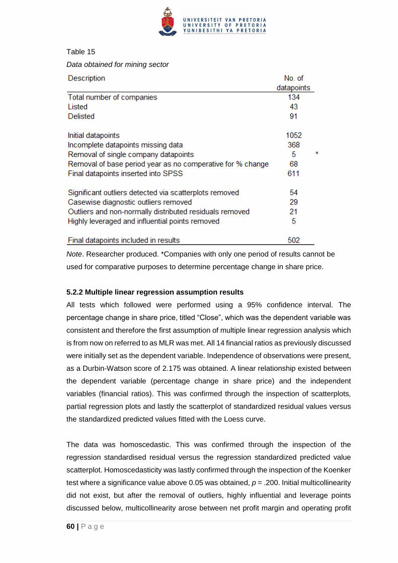
60 | P a g e
Table 15 Data obtained for mining sector
Data obtained for mining sector
Note. Researcher produced. *Companies with only one period of results cannot be
used for comparative purposes to determine percentage change in share price.
5.2.2 Multiple linear regression assumption results
All tests which followed were performed using a 95% confidence interval. The
percentage change in share price, titled “Close”, which was the dependent variable was
consistent and therefore the first assumption of multiple linear regression analysis which
is from now on referred to as MLR was met. All 14 financial ratios as previously discussed
were initially set as the dependent variable. Independence of observations were present,
as a Durbin-Watson score of 2.175 was obtained. A linear relationship existed between
the dependent variable (percentage change in share price) and the independent
variables (financial ratios). This was confirmed through the inspection of scatterplots,
partial regression plots and lastly the scatterplot of standardized residual values versus
the standardized predicted values fitted with the Loess curve.
The data was homoscedastic. This was confirmed through the inspection of the
regression standardised residual versus the regression standardized predicted value
scatterplot. Homoscedasticity was lastly confirmed through the inspection of the Koenker
test where a significance value above 0.05 was obtained, p = .200. Initial multicollinearity
did not exist, but after the removal of outliers, highly influential and leverage points
discussed below, multicollinearity arose between net profit margin and operating profit

61 | P a g e
margin. Operating profit margin possessed the highest VIF score (12.793) and lowest
tolerance factor (0.078) and was therefore removed. No multicollinearity was further
detected for the variables as all VIF scores were below 10, indicating insignificant
multicollinearity.
See Table 15 where a summary was made of the number of outliers, highly influential
and highly leveraged points which were discussed below. 54 significant outliers were
firstly removed by the inspection of scatterplots and by applying professional judgement
to these scatterplots. Secondly, 29 outliers were removed by way of running and
rerunning case wise diagnostics in the normal regression mode until no outliers were
detected which were more than three standard deviations. Further, 21 extreme outliers
and residuals were removed by detecting these via the inspection of a combination of
the extreme values (outlier) function and the normality box-plot in SPSS. Five highly
leveraged and influential points were identified and removed. Even though some
additional points remained which were situated above other points on the Cook’s
Distance vs Centred Leveraged Value graph, the combination of their Cook’s and
leverage rating would not have led to significant influence or leverage (See Appendix B)
(IBM Corporation, n.d.).
Lastly, the normal distribution of the residuals was ensured. This was confirmed by
inspecting the histogram of regression standardized residuals and by inspecting the
normal P-P plot of regression standardized residuals. Further, the skewness and kurtosis
value of the normal regression standardized, and unstandardized residuals both
amounted to 0.268 and -0.306 respectively, which were less than ± 0.5, indicating
approximate normal distribution. The Shapiro-Wilk test on both the standardized and
unstandardized residuals however did not deliver a significance value above 0.05.
As indicated by Hair et al. (2010) and Kim (2013), the Shapiro-Wilk test could be
oversensitive to large populations and could lead to unreliable results. Kim (2013)
indicated that these large samples are classified as any population with more than 300
datapoints. In this instance the mining sector contained the largest population of 502
datapoints, followed by the real estate investment trusts sector, which was the second
largest sector, with 284 datapoints. Seeing that the inspection of the histogram of
regression standardized residuals and normal P-P plot of regression standardized
residuals strongly indicated that the residuals were approximately normally distributed,
the opposite finding delivered by the Shapiro-Wilk test appears to have been due to the
large population of more than 300 as indicated by Kim (2013). To further confirm the

62 | P a g e
approximate normality of the residuals, the normal Q-Q plot and Box plot was inspected,
where all indicated that the residuals were approximately normally distributed.
After performance of the tests discussed above, a final total of 502 datapoints out of the
initial 1052 datapoints were fit for testing purposes, as these met all eight of the multiple
linear regression assumptions. The final stepwise multiple linear regression test followed
in which all 502 datapoints were included. Please refer to the first section of Appendix B
under Hypothesis 1 for all the IBM SPSS v25 outputs and other detail to support the
results which were discussed above for each of the eight assumptions of multiple linear
regression analysis.
5.2.3 Descriptive statistics
Table 16 provides a summary of the most important descriptive statistics derived from
the final 502 datapoints which were produced from the normal multiple linear regression
model after meeting the eight multiple linear regression assumptions. As part of the
descriptive statistics, the Pearson correlation and its significance were included. 11 of
the 13 financial ratios displayed statistically significant correlations with share price
performance. A Pearson correlation however does not take into account the combined
effect of the other financial ratios on the dependent variable when determining a
correlation and therefore provides less concrete evidence when compared to performing
a multiple regression model. The return on equity ratio produced the most statistically
significant Pearson correlation with the percentage change in share price.

63 | P a g e
Table 16 Descriptive statistics: Mining
Descriptive statistics: Mining
Note. Researcher produced. M = Mean, SD = Standard deviation, N = Population size,
r = Pearson correlation, p = significance.
5.2.4 Stepwise multiple linear regression results
Table 17 provides a summary of the results of the automatic stepwise multiple linear
regression performed in IBM SPSS v25. A stepwise multiple linear regression takes the
effect of all variables entered into account to find the model, from multiple combinations,
with the most explanatory power (George & Mallery, 2019; Hair et al., 2010). Some
variables might therefore have statistically significant relationships with the dependent
variable on an individual basis, but when added to the equation do not increase the
adjusted coefficient of determination (adjusted R2). These variables would therefore not
be included as part of the multiple linear regression equation.

64 | P a g e
The ratios provided in Table 17 were therefore the ratios which in combination delivered
the highest adjusted R2 for the sector. The stepwise multiple linear regression was
performed at the 95% confidence interval where these findings were displayed in order
of the most significant financial ratios to the least significant. Return on equity delivered
the most significant effect on the percentage change in the share price, where total asset
turnover delivered the least significant.
Table 17 Automatic stepwise regression results: Mining
Automatic stepwise regression results: Mining
Note. Researcher produced. β = Unstandardized coefficients beta, CSE =
Unstandardized coefficient standard error, Beta = standardised coefficient beta, t = t -
statistic, p = significance.
The combined model achieved a coefficient of determination (R2) value of 0.234 and an
adjusted coefficient of determination (adjusted R2) value of 0.225. 22.5% of the variation
in share prices could therefore possibly be explained by the six financial ratios as
indicated in Table 17. The analysis of variance (ANOVA) showed that the effect of the
change in financial ratios was statistically significant on the share price performance at
the 95% confidence level, F(6,495) = 25.221, p = .000.
Please refer to the second section of Appendix B under Hypothesis 1 for the relevant
IBM SPSS v25 outputs and other detail to support the automatic stepwise multiple linear
regression results discussed above.

65 | P a g e
5.2.5 Result
Based on the results discussed above, rejection of the null hypothesis and acceptance
of the alternative hypothesis was appropriate.
• Alternate hypothesis two (H11): Significant statistical relationships exist between
at least one or more financial ratios and the share price performance of the mining
sector on the JSE.
5.3 Hypothesis 2: Banking
Research question two (RQ2): Do statistical relationships exist between financial
ratios and share price performance of the banking sector on the JSE?
• Null hypothesis two (H02): No significant statistical relationships exist between
any financial ratios and the share price performance of the banking sector on the
JSE.
• Alternate hypothesis two (H12): Significant statistical relationships exist between
at least one or more financial ratios and the share price performance of the
banking sector on the JSE.
5.3.1 Description of data obtained and cleaned
The full dataset from 1 January 1997 to 30 September 2018 for the ICB level 3 Banking
sector was obtained and cleaned as displayed in Table 18. This table includes the
details around items that were removed from the dataset which is further

66 | P a g e
Table 18 Data obtained for banking sector
Data obtained for banking sector
Note. Researcher produced.
5.3.2 Multiple linear regression assumption results
All tests which followed were performed using a 95% confidence interval. The
percentage change in share price, titled “Close”, which was the dependent variable was
consistent and therefore the first assumption of multiple linear regression analysis which
is from now on referred to as MLR was met. All 14 financial ratios as previously discussed
were initially attempted to be extracted, but only 11 of the 14 chosen financial ratios were
available as dependent variables with figures from the Iress Expert Database. The
banking industry does not generate turnover or revenue as generally defined as most
income is derived from interest income and other sources and therefore these ratios are
not common within the selected industry. No operating margins, net profit margins or
total asset turnover ratios were therefore available on the database and were therefore
not included.
Independence of observations were present, as a Durbin-Watson score of 2.157 was
obtained. A linear relationship existed between the dependent variable (percentage
change in share price) and the independent variables (financial ratios). This was
confirmed through the inspection of scatterplots, partial regression plots and lastly the
scatterplot of standardized residual values versus the standardized predicted values
67 | P a g e
fitted with the Loess curve. The data was homoscedastic. This was confirmed through
the inspection of the regression standardised residual versus the regression
standardized predicted value scatterplot. Homoscedasticity was lastly confirmed through
the inspection of the Koenker test where a significance value above 0.05 was obtained,
p = .071. No significant multicollinearity existed as constant VIF scores of far below 10
existed.
See Table 18 where a summary was made of the number of outliers, highly influential
and highly leveraged points which were discussed below. 13 significant outliers were
firstly removed by the inspection of scatterplots and by applying professional judgement
to these scatterplots. Secondly, five outliers were removed by way of running and
rerunning case wise diagnostics in the normal regression mode until no outliers were
detected which were more than three standard deviations. Further, five extreme outliers
and residuals were removed by detecting these via the inspection of a combination of
the extreme values (outlier) function and the normality box-plot in SPSS. Eight highly
leveraged and influential points were identified and removed. Even though some
additional points remained which were situated above other points on the Cook’s
Distance vs Centred Leveraged Value graph, the combination of their Cook’s and
leverage rating would not have led to significant influence or leverage (See Appendix B)
(IBM Corporation, n.d.).
Lastly, the normal distribution of the residuals was ensured. This was confirmed by
inspecting the histogram of regression standardized residuals and by inspecting the
normal P-P plot of regression standardized residuals. The skewness and kurtosis value
of the normal regression standardized, and unstandardized residuals both amounted to
0.457 and -0.173 respectively, which were less than ± 0.5, indicating approximate normal
distribution. The Shapiro-Wilk test on both the standardized and unstandardized
residuals delivered a significance value above 0.05 which further substantiated the
normality of the regression model, p = .058. To further confirm the approximate normality
of the residuals, the normal Q-Q plot and Box plot was inspected, where all indicated
that the residuals were approximately normally distributed. In the final Box plot some
residuals occurred above the main grouping of box plot residuals but seeing these were
not significant, the Shapiro-Wilk score was above significance, and various other
residuals had already been removed before these, no significant outlier of residuals were
identified. No further action was deemed necessary.

68 | P a g e
After performance of the tests discussed above, a final total of 109 datapoints out of the
initial 158 datapoints were fit for testing purposes, as these met all eight of the multiple
linear regression assumptions. The final stepwise multiple linear regression test followed
in which all 109 datapoints were included. Please refer to the first section of Appendix B
under Hypothesis 2 for all the IBM SPSS v25 outputs and other detail to support the
results which were discussed above for each of the eight assumptions of multiple linear
regression analysis.
5.3.3 Descriptive statistics
Table 19 provides a summary of the most important descriptive statistics derived from
the final 109 datapoints which were produced from the normal multiple linear regression
model after meeting the eight multiple linear regression assumptions. As part of the
descriptive statistics, the Pearson correlation and its significance were included. 3 of the
11 financial ratios displayed statistically significant correlations with share price
performance. A Pearson correlation however does not take into account the combined
effect of the other financial ratios on the dependent variable when determining a
correlation and therefore provides less concrete evidence when compared to performing
a multiple regression model. The price-earnings ratio produced the most significant
Pearson correlation with the percentage change in the share price.

69 | P a g e
Table 19 Descriptive statistics: Banking
Descriptive statistics: Banking
Note. Researcher produced. M = Mean, SD = Standard deviation, N = Population size,
r = Pearson correlation, p = significance.
5.3.4 Stepwise multiple linear regression results
Table 20 provides a summary of the results of the automatic stepwise multiple linear
regression performed in IBM SPSS v25. A stepwise multiple linear regression takes the
effect of all variables entered into account to find the model, from multiple combinations,
with the most explanatory power (George & Mallery, 2019; Hair et al., 2010). Some
variables might therefore have statistically significant relationships with the dependent
variable on an individual basis, but when added to the equation do not increase the
adjusted coefficient of determination (adjusted R2). These variables would therefore not
be included as part of the multiple linear regression equation. The ratios provided in
Table 20 were therefore the ratios which in combination delivered the highest adjusted
R2 for the sector. The stepwise multiple linear regression was performed at the 95%
confidence interval where these findings were displayed in order of the most significant
financial ratios to the least significant. Price-earnings delivered the most significant effect

70 | P a g e
on the percentage change in the share price, where return on equity delivered the least
significant.
Table 20 Automatic stepwise regression results: Banking
Automatic stepwise regression results: Banking
Note. Researcher produced. β = Unstandardized coefficients beta, CSE =
Unstandardized coefficient standard error, Beta = standardised coefficient beta, t = t -
statistic, p = significance
The combined model achieved a coefficient of determination (R2) of 0.196 and an
adjusted coefficient of determination (adjusted R2) value of 0.181. 18.1% of the variation
in share prices could therefore possibly be explained by the two financial ratios as
indicated in Table 20. The analysis of variance (ANOVA) showed that the effect of the
change in financial ratios was significant on the share price performance at the 95%
confidence level, F(2,108) = 12.940, p = .000.
Please refer to the second section of Appendix B under Hypothesis 2 for the relevant
IBM SPSS v25 outputs and other detail to support the automatic stepwise multiple linear
regression results discussed above.
5.3.5 Result
Based on the results discussed above, rejection of the null hypothesis and acceptance
of the alternative hypothesis was appropriate.
• Alternate hypothesis two (H12): Significant statistical relationships exist between
at least one or more financial ratios and the share price performance of the
banking sector on the JSE.
5.4 Hypothesis 3: Life Insurance
Research question two (RQ1): Do statistical relationships exist between financial
ratios and share price performance of the life insurance sector on the JSE?

71 | P a g e
• Null hypothesis two (H01): No significant statistical relationships exist between
any financial ratios and the share price performance of the life insurance sector
on the JSE.
• Alternate hypothesis two (H11): Significant statistical relationships exist between
at least one or more financial ratios and the share price performance of the life
insurance sector on the JSE.
5.4.1 Description of data obtained and cleaned
The full dataset from 1 January 1997 to 30 September 2018 for the ICB level 3 life
insurance sector was obtained and cleaned for multiple linear regression purposes as
displayed in Table 21.
Table 21 Data obtained for life insurance sector
Data obtained for life insurance sector
Note. Researcher Produced.
5.4.2 Multiple linear regression assumption results
All tests which followed were performed using a 95% confidence interval. The
percentage change in share price, titled “Close”, which was the dependent variable was
consistent and therefore the first assumption of multiple linear regression analysis which
is from now on referred to as MLR was met. All 14 financial ratios as previously discussed
were initially set as the dependent variable. Independence of observations were present,
as a Durbin-Watson score of 1.769 was obtained. A linear relationship existed between

72 | P a g e
the dependent variable (percentage change in share price) and the independent
variables (financial ratios). This was confirmed through the inspection of scatterplots,
partial regression plots and lastly the scatterplot of standardized residual values versus
the standardized predicted values fitted with the Loess curve.
The data was homoscedastic. This was confirmed through the inspection of the
regression standardised residual versus the regression standardized predicted value
scatterplot. Homoscedasticity was lastly confirmed through the inspection of the Koenker
value where a significance value above 0.05 was obtained, p = .262. Initial
multicollinearity was detected. Return on Assets % presented a VIF score of 23.374 and
a tolerance of 0.043. This variable was removed, and multicollinearity was again
inspected. Another variable namely Return on Capital Employed %, subsequently
developed a VIF score of 10.525 and a tolerance of 0.095. This variable was also
removed. The tests were rerun and further, no significant multicollinearity was detected
as all the variables presented a VIF score of less than 10, and a tolerance value of more
than 0.1, indicating insignificant multicollinearity. 12 independent variables remained.
See Table 21 where a summary was made of the number of outliers, highly influential
and highly leveraged points which were discussed below. 11 significant outliers were
removed by the inspection of scatterplots and by applying professional judgement to
these scatterplots. No significant outliers were detected by using the case wise
diagnostics function in SPSS. No extreme outliers and residuals were removed as none
were detected via the inspection of a combination of the extreme values (outlier) function
and the normality box-plot in SPSS. Two highly leveraged and influential points were
identified and removed. Even though some additional points remained which were
situated above other points on the Cook’s Distance vs Centred Leveraged Value graph,
the combination of their Cook’s and leverage rating would not have led to significant
influence or leverage (See Appendix B) (IBM Corporation, n.d.).
The normal distribution of the residuals was ensured. This was confirmed by inspecting
the histogram of the regression standardized residuals and by inspecting the normal P-
P plot of regression standardized residuals. Further, the skewness and kurtosis value of
the normal regression standardized, and unstandardized residuals both amounted to
0.055 and -0.220 respectively, which were less than ± 0.5, indicating approximate normal
distribution. The Shapiro-Wilk test on both the standardized and unstandardized
residuals further delivered a significance value above 0.05, indicating to the normality of
residuals, p = .732. To further confirm the approximate normality of the residuals, the

73 | P a g e
normal Q-Q plot and Box plot was inspected, where all indicated that the residuals were
approximately normally distributed.
After performance of the tests discussed above, a final total of 85 datapoints out of the
initial 143 datapoints were fit for testing purposes, as these met all eight of the multiple
linear regression assumptions. The final stepwise multiple linear regression test followed
in which all 85 datapoints were included. Please refer to the first section of Appendix B
under Hypothesis 3 for all the IBM SPSS v25 outputs and other detail to support the
results which were discussed above for each of the eight assumptions of multiple linear
regression analysis.
5.4.3 Descriptive statistics
Table 22 provides a summary of the most important descriptive statistics derived from
the final 85 datapoints which were produced from the normal multiple linear regression
model after meeting the eight multiple linear regression assumptions. As part of the
descriptive statistics, the Pearson correlation and its significance were included. 3 of the
12 financial ratios displayed statistically significant correlations with share price
performance. A Pearson correlation however does not take into account the combined
effect of the other financial ratios on the dependent variable when determining a
correlation and therefore provides less concrete evidence when compared to performing
a multiple regression model. Operating profit margin produced the most significant
Pearson correlation with the percentage change in the share price.

74 | P a g e
Table 22 Descriptive statistics: Life Insurance
Descriptive statistics: Life Insurance
Note. Researcher produced. M = Mean, SD = Standard deviation, N = Population size,
r = Pearson correlation, p = significance.
5.4.4 Stepwise multiple linear regression results
Table 23 provides a summary of the results of the automatic stepwise multiple linear
regression performed in IBM SPSS v25. A stepwise multiple linear regression takes the
effect of all variables entered into account to find the model, from multiple combinations,
with the most explanatory power (George & Mallery, 2019; Hair et al., 2010). Some
variables might therefore have statistically significant relationships with the dependent
variable on an individual basis, but when added to the equation do not increase the
adjusted coefficient of determination (adjusted R2). These variables would therefore not
be included as part of the multiple linear regression equation. The operating margin ratio

75 | P a g e
provided in Table 23 was therefore the only ratio which after considering the effect of the
other available ratios delivered the highest adjusted R2 for the sector. The stepwise
multiple linear regression was performed at the 95% confidence interval.
Table 23 Automatic stepwise regression results: Life Insurance
Automatic stepwise regression results: Life Insurance
Note. Researcher produced. β = Unstandardized coefficients beta, CSE =
Unstandardized coefficient standard error, Beta = standardised coefficient beta, t = t -
statistic, p = significance
The combined model achieved a coefficient of determination (R2) value of 0.073 and an
adjusted coefficient of determination (adjusted R2) value of 0.061. 6.1% of the variation
in share prices could therefore possibly be explained by the operating profit margin %.
The analysis of variance (ANOVA) showed that the effect of the change in financial ratios
was statistically significant on the share price performance at the 95% confidence level,
F(1,83) = 6.494, p = .013.
Please refer to the second section of Appendix B under Hypothesis 3 for the relevant
IBM SPSS v25 outputs and other detail to support the automatic stepwise multiple linear
regression results discussed above.
5.4.5 Result
Based on the results discussed above, rejection of the null hypothesis and acceptance
of the alternative hypothesis was appropriate.
• Alternate hypothesis two (H11): Significant statistical relationships exist between
at least one or more financial ratios and the share price performance of the life
insurance sector on the JSE.
5.5 Hypothesis 4: Real Estate Investment Trusts
Research question two (RQ1): Do statistical relationships exist between financial
ratios and share price performance of the real estate investment trusts sector on the
JSE?

76 | P a g e
• Null hypothesis two (H01): No significant statistical relationships exist between
any financial ratios and the share price performance of the real estate investment
trusts sector on the JSE.
• Alternate hypothesis two (H11): Significant statistical relationships exist between
at least one or more financial ratios and the share price performance of the real
estate investment trusts sector on the JSE.
5.5.1 Description of data obtained and cleaned
The full dataset from 1 January 1997 to 30 September 2018 for the ICB level 3 real
estate investment trusts sector was obtained and cleaned for multiple linear regression
purposes as displayed in Table 24.
Table 24 Data obtained for real estate investment trusts sector
Data obtained for real estate investment trusts sector
Note. Researcher Produced. *Companies with only one period of results cannot be
used for comparative purposes to determine percentage change in share price.
5.5.2 Multiple linear regression assumption results
All tests which followed were performed using a 95% confidence interval. The
percentage change in share price, titled “Close”, which was the dependent variable was
consistent and therefore the first assumption of multiple linear regression analysis which
is from now on referred to as MLR was met. All 14 financial ratios as previously discussed

77 | P a g e
were initially set as the dependent variable. Independence of observations were present,
as a Durbin-Watson score of 2.124 was obtained. A linear relationship existed between
the dependent variable (percentage change in share price) and the independent
variables (financial ratios). This was confirmed through the inspection of scatterplots,
partial regression plots and lastly the scatterplot of standardized residual values versus
the standardized predicted values fitted with the Loess curve.
Initial multicollinearity was detected. Return on Assets % presented a VIF score of
30.892 and a tolerance score of 0.032 and was removed. Various other variables also
presented substantial VIF and tolerance scores, but on each test only one variable was
removed per test, after which the normal regression was rerun and inspected to
determine the effect of the variable removal on multicollinearity. Debt to Equity presented
a VIF score of 226.334 and tolerance score of 0.045 and was removed. After rerunning
the multiple linear regression, Net Profit Margin % presented a VIF score of 11.188 and
tolerance score of 0.080 and was removed. After this no VIF or tolerance scores above
10 or below 0.1 respectively were detected indicating that no multicollinearity remained.
In total three variables were removed due to multicollinearity issues.
See Table 24 where a summary was made of the number of outliers, highly influential
and highly leveraged points which were discussed below. 28 significant outliers were
firstly removed by the inspection of scatterplots and by applying professional judgement
to these scatterplots. Secondly, two outliers were removed by way of running and
rerunning case wise diagnostics in the normal regression mode until no outliers were
detected which were more than three standard deviations. Further, four extreme outliers
and residuals were removed by detecting these with a combination of the extreme values
(outlier) function and the normality box-plot in SPSS. No highly leveraged and influential
points were identified or removed. Even though some additional points were noted which
were situated above other points on the Cook’s Distance vs Centred Leveraged Value
graph, the combination of their Cook’s and leverage rating would not have led to
significant influence or leverage (See Appendix B) (IBM Corporation, n.d.).
The normal distribution of the residuals was ensured. This was confirmed by inspecting
the histogram of the regression standardized residuals and by inspecting the normal P-
P plot of regression standardized residuals. Further, the skewness and kurtosis value of
the normal regression standardized, and unstandardized residuals both amounted to
0.268 and -0.181 respectively, which were less than ± 0.5, indicating approximate normal
distribution. The Shapiro-Wilk test on both the standardized and unstandardized
78 | P a g e
residuals delivered a significance value above 0.05 which further substantiated the
normality of the regression model, p = .083. To further confirm the approximate normality
of the residuals, the normal Q-Q plot and Box plot was inspected, where all indicated
that the residuals were approximately normally distributed.
Homoscedasticity procedures
In terms of the fifth assumption of multiple linear regression testing, the data is required
to be homoscedastic. If the data is not homoscedastic, then it is classified as
heteroscedastic. Some of the data variables initially displayed heteroscedastic
characteristics. When performing the Koenker test on all the input data, a significance
score of below 0.05 was obtained, p = .004. To determine precisely which variable
contained data which was heteroscedastic, the Koenker test was performed for each
independent variable. Out of the remaining 11 variables, after the removal of variables
with multicollinearity as discussed above, two of the variables namely dividend yield and
debt to assets presented significance values of less than 0.05, indicating that
heteroscedasticity was present, p = .005, p = .029.
According to Hair et al. (2010), heteroscedasticity could possibly be solved by
transforming the affected data. When determining how to solve heteroscedastic data,
the scatterplot should be inspected to determine if a cone shaped distribution exists. If
the cone opens to the right side of the distribution, then the data should be transformed
using the inverse. If the cone opens to the left side of the distribution, then a square root
transformation is most appropriate (Hair et al., 2010). Debt to assets opened to the right
side and therefore an inverse transformation was performed which improved the
homoscedasticity of the data by delivering a significance value of more than 0.05, p =
.211. The new inverse transformation variable created from the debt to assets ratio
variable was titled INV_DA_3.
Dividend yield opened to the left side seeing that a great number of dividend yield ratios
were situated on the 0% points, as no dividends were paid by most of the companies. A
square root transformation was performed, but the heteroscedasticity of this transformed
variable decreased as a lower significance value than previously calculated before
transformation was obtained, p = .003. Power transformations were also attempted but
even though this improved the significance value, it still did not deliver a significance
value of more than 0.05 and therefore, a transformation was not performed, p = .040.
Other possible transformations were investigated, as indicated by Hair et al. (2010), but
these could not be executed due to the presence of zero values in the variable data.

79 | P a g e
Inverse transformations could not be performed as no values could be divided by zero
without data errors. Logarithm transformation could also not be performed as the
presence of zero values also provided data errors. Lastly, Hair et al. (2010) discussed
the use of arcsin transformations which are best suited for the transformation of
proportions. Even though this was not the best method to use for the data, it was
attempted, but also delivered data errors as data with a value of greater than one, could
not be transformed using the arcsin transformation. Seeing that transformations
attempted did not improve the homoscedasticity of the data and the variable did not
present a strong linear function in comparison with the dependent variable, it was seen
best fit to remove the dividend yield variable. After the removal of the dividend yield
variable and the transformation of the debt to assets variable, the Koenker test delivered
a significance value of more than 0.05 and the data was deemed as homoscedastic, p =
.166. Homoscedasticity was further confirmed through the inspection of the regression
standardised residuals versus the regression standardized predicted value scatterplot
which indicated that the data was homoscedastic.
After performance of the tests discussed above, a final total of 284 datapoints out of the
initial 427 were fit for testing purposes, as these met all eight of the multiple linear
regression assumptions. The final stepwise multiple linear regression test followed in
which all 284 datapoints were included. Please refer to the first section of Appendix B
under Hypothesis 4 for all the IBM SPSS v25 outputs and other detail to support the
results which were discussed above for each of the eight assumptions of multiple linear
regression analysis.
5.5.3 Descriptive statistics
Table 25 provides a summary of the most important descriptive statistics derived from
the final 284 datapoints which were produced from the normal multiple linear regression
model after meeting the eight multiple linear regression assumptions. As part of the
descriptive statistics, the Pearson correlation and its significance were included. 6 of the
10 financial ratios displayed statistically significant correlations with share price
performance. A Pearson correlation however does not take into account the combined
effect of the other financial ratios when determining a correlation and therefore provides
less concrete evidence when compared to performing a normal or stepwise multiple
regression. Operating profit margin produced the most significant Pearson correlation
with the percentage change in the share price.

80 | P a g e
Table 25 Descriptive statistics: Real Estate Investment Trusts
Descriptive statistics: Real Estate Investment Trusts
Note. Researcher produced. M = Mean, SD = Standard deviation, N = Population size,
r = Pearson correlation, p = significance. Operating Profit Margin produced the most
significant Pearson correlation with the percentage change in share price. INV_DA_3 is
the inverse transformation variable of the debt to asset ratio as discussed in section
5.5.2.
5.5.4 Stepwise multiple linear regression results
Table 26 provides a summary of the results of the automatic stepwise multiple linear
regression performed in IBM SPSS v25. A stepwise multiple linear regression takes the
effect of all variables entered into account to find the model, from multiple combinations,
with the most explanatory power (George & Mallery, 2019; Hair et al., 2010). Some
variables might therefore have statistically significant relationships with the dependent
variable on an individual basis, but when added to the equation do not increase the
adjusted coefficient of determination (adjusted R2). These variables would therefore not
be included as part of the multiple linear regression equation. The ratios provided in

81 | P a g e
Table 26 were therefore the ratios which in combination delivered the highest adjusted
R2 for the sector. The stepwise multiple linear regression was performed at the 95%
confidence interval where these findings were displayed in order of the most significant
financial ratios to the least significant. Operating profit margin delivered the most
significant effect on the percentage change in the share price, where return on equity
delivered the least significant.
Table 26 Automatic stepwise regression results: Real Estate Investment Trusts
Automatic stepwise regression results: Real Estate Investment Trusts
Note. Researcher produced. β = Unstandardized coefficients beta, CSE =
Unstandardized coefficient standard error, Beta = standardised coefficient beta, t = t -
statistic, p = significance
The combined model achieved a coefficient of determination (R2) value of 0.271 and an
adjusted coefficient of determination (adjusted R2) value of 0.263. 26.3% of the variation
in share prices could therefore possibly be explained by the three financial ratios as
indicated in Table 26. The analysis of variance (ANOVA) showed that the effect of the
change in financial ratios was statistically significant on the share price performance at
the 95% confidence level, F(3,280) = 34.748, p = .000.
Please refer to the second section of Appendix B under Hypothesis 4 for the relevant
IBM SPSS v25 outputs and other detail to support the automatic stepwise multiple linear
regression results discussed above.
5.5.5 Result
Based on the results discussed above, rejection of the null hypothesis and acceptance
of the alternative hypothesis was appropriate.
• Alternate hypothesis two (H11): Significant statistical relationships exist between
at least one or more financial ratios and the share price performance of the real
estate investment trust sector on the JSE.

82 | P a g e
5.6 Hypothesis 5: Mobile Telecommunications
Research question two (RQ1): Do statistical relationships exist between financial ratios
and share price performance of the mobile telecommunications sector on the JSE?
• Null hypothesis two (H01): No significant statistical relationships exist between
any financial ratios and the share price performance of the mobile
telecommunications sector on the JSE.
• Alternate hypothesis two (H11): Significant statistical relationships exist between
at least one or more financial ratios and the share price performance of the mobile
telecommunications sector on the JSE.
5.6.1 Description of data obtained and cleaned
The full dataset from 1 January 1997 to 30 September 2018 for the ICB level 3 mobile
telecommunications sector was obtained and cleaned for multiple linear regression
purposes as displayed in Table 27.
Table 27 Data obtained for mobile telecommunications sector
Data obtained for mobile telecommunications sector
Note. Researcher Produced.
5.6.2 Multiple linear regression assumption results
All tests which followed were performed using a 95% confidence interval. The
percentage change in share price, titled “Close”, which was the dependent variable was
83 | P a g e
consistent and therefore the first assumption of multiple linear regression analysis which
is from now on referred to as MLR was met. All 14 financial ratios as previously discussed
were initially set as the dependent variable. Independence of observations were present,
as a Durbin-Watson score of 1.665 was obtained. A linear relationship existed between
the dependent variable (percentage change in share price) and the independent
variables (financial ratios). This was confirmed through the inspection of scatterplots,
partial regression plots and lastly the scatterplot of standardized residual values versus
the standardized predicted values fitted with the Loess curve. The data was
homoscedastic. This was confirmed through the inspection of the regression
standardised residual versus the regression standardized predicted values scatterplot.
Homoscedasticity was lastly confirmed through the inspection of the Koenker test where
a significance value above 0.05 was obtained, p = .259.
Initial multicollinearity was detected. Return on Equity % presented a VIF score of 92.621
and a tolerance score of 0.011 and was removed. Various other variables also presented
substantial VIF and tolerance scores, but on each test only one variable was removed
per test, after which the normal regression was rerun and inspected to determine the
effect of the variable removal on multicollinearity. Operating Profit Margin % presented
a VIF score of 26.811 and tolerance score of 0.037 and was removed. After rerunning
the multiple linear regression, price-to-book value presented a VIF score of 13.764 and
tolerance score of 0.073 and was removed. After this no VIF or tolerance scores above
10 or below 0.1 respectively were detected until the removal of highly leveraged and
influential points occurred, after which Net Profit Margin % presented a VIF score of
12.370 and a VIF score of 0.081. This variable was lastly removed after which no more
significant multicollinearity remained. In total four variables were removed, and 10
variables remained.
See Table 27 where a summary was made of the number of outliers, highly influential
and highly leveraged points which were discussed below. Nine significant outliers were
firstly removed by the inspection of scatterplots and by applying professional judgement
to these scatterplots. No outliers were detected via performing case wise diagnostics.
Five highly leveraged and influential points were identified and removed. Even though
some additional points remained which were situated above other points on the Cook’s
Distance vs Centred Leveraged Value graph, the combination of their Cook’s and
leverage rating would not have led to significant influence or leverage (See Appendix B)
(IBM Corporation, n.d.).

84 | P a g e
Lastly, the normal distribution of the residuals was ensured. This was confirmed by
inspecting the histogram of the regression standardized residuals and by inspecting the
normal P-P plot of regression standardized residuals. Further, the skewness and kurtosis
value of the normal regression standardized, and unstandardized residuals both
amounted to 0.163 and -0.519 respectively. Even though the kurtosis values were just
above the ± 0.5 rule of thumb, the Shapiro-Wilk test on both the standardized and
unstandardized residuals delivered a substantial significance value above 0.05, which
indicates that the residuals were normally distributed, p = .529. To further confirm the
approximate normality of the residuals, the normal Q-Q plot and Box plot was inspected,
where all indicated that the residuals were approximately normally distributed.
After performance of the tests discussed above, a final total of 49 datapoints out of the
initial 73 were fit for testing purposes, as these met all eight of the multiple linear
regression assumptions. The final stepwise multiple linear regression test followed in
which all 49 datapoints were included. Please refer to the first section of Appendix B
under Hypothesis 5 for all the IBM SPSS v25 outputs and other detail to support the
results which were discussed above for each of the eight assumptions of multiple linear
regression analysis.
5.6.3 Descriptive statistics
Table 28 provides a summary of the most important descriptive statistics derived from
the final 49 datapoints which were produced from the normal multiple linear regression
model after meeting the eight multiple linear regression assumptions. As part of the
descriptive statistics, the Pearson correlation and its significance were included. 3 of the
10 financial ratio displayed statistically significant correlations with share price
performance. A Pearson correlation however does not take into account the combined
effect of the other financial ratios when determining a correlation and therefore provides
less concrete evidence when compared to performing a normal or stepwise multiple
regression. The return on assets ratio produced the most significant Pearson correlation
with the percentage change in the share price.

85 | P a g e
Table 28 Descriptive statistics: Mobile Telecommunications
Descriptive statistics: Mobile Telecommunications
Note. Researcher produced. M = Mean, SD = Standard deviation, N = Population size,
r = Pearson correlation, p = significance.
5.6.4 Stepwise multiple linear regression results
Table 29 provides a summary of the results of the automatic stepwise multiple linear
regression performed in IBM SPSS v25. A stepwise multiple linear regression takes the
effect of all variables entered into account to find the model, from multiple combinations,
with the most explanatory power (George & Mallery, 2019; Hair et al., 2010). Some
variables might therefore have statistically significant relationships with the dependent
variable on an individual basis, but when added to the equation do not increase the
adjusted coefficient of determination (adjusted R2). These variables would therefore not
be included as part of the multiple linear regression equation. The ratios provided in
Table 29 were therefore the ratios which in combination delivered the highest adjusted
R2 for the sector. The stepwise multiple linear regression was performed at the 95%
confidence interval where these findings were displayed in order of the most significant
financial ratios to the least significant. Return on assets delivered the most significant
effect on the percentage change in the share price, where the debt to assets ratio
delivered the least significant.

86 | P a g e
Table 29 Automatic stepwise regression results: Mobile Telecommunications
Automatic stepwise regression results: Mobile Telecommunications
Note. Researcher produced. β = Unstandardized coefficients beta, CSE =
Unstandardized coefficient standard error, Beta = standardised coefficient beta, t = t -
statistic, p = significance.
The combined model achieved a coefficient of determination (R2) value of 0.43 and an
adjusted coefficient of determination (adjusted R2) value of 0.392. 39.2% of the variation
in share prices could therefore possibly be explained by the three financial ratios as
indicated in Table 29. The analysis of variance (ANOVA) showed that the effect of the
change in financial ratios was statistically significant on the share price performance at
the 95% confidence level, F(3,45) = 11.295, p = .000.
Please refer to the second section of Appendix B under Hypothesis 5 for the relevant
IBM SPSS v25 outputs and other detail to support the automatic stepwise multiple linear
regression results discussed above.
5.6.5 Result
Based on the results discussed above, rejection of the null hypothesis and acceptance
of the alternative hypothesis was appropriate.
• Alternate hypothesis two (H11): Significant statistical relationships exist between
at least one or more financial ratios and the share price performance of the mobile
telecommunications sector on the JSE.
5.7 Summary of results
Table 30 provides a summary of the stepwise multiple regression results for each of the
five hypotheses tested. First the overall outcome of either the acceptance or rejection of
the nul hypothesis was presented. The coefficient of determination (R2) and adjusted
coefficient of determination (adjusted R2) was then provided. The most significant

87 | P a g e
financial ratios which had a statistically significant relationship with the percentage
change in the share price was then provided in order of beta weight and significance
value. Mobile telecommunications had the highest adjusted coefficient of determination
out of all five sectors tested which indicates that the highest variation in percentage
change in share prices could be explained by financial ratios in this sector.
Table 30 Summary of stepwise multiple linear regression results
Summary of stepwise multiple linear regression results
Note. Researcher produced. R2 = coefficient of determination, Adjusted R2 = adjusted
coefficient of determination, Beta = standardised coefficient beta, p = significance.
88 | P a g e
CHAPTER 6 DISCUSSION OF RESULTS
6.1 Introduction
This chapter provides a discussion of the results as presented in Chapter 5 per
hypothesis as documented in Chapter 3. The discussion links the results with the
literature, theories and results obtained by other researchers as documented in Chapters
1 and 2. The aim of this research was to determine if statistically significant relationships
exist between financial ratios and share price performance of the top five sectors on the
Johannesburg Stock Exchange (JSE), based on market capitalisation. These were the
mining, banking, life insurance, real estate investment trust and mobile
telecommunication sectors.
The aim of the research was met as each of the five sectors contained the appropriate
data to perform multiple linear regression analysis. The research was performed using
14 of the most commonly and documented financial ratios, as determined by academic
literature, of which 10 were financial accounting ratios and four price-to-fundamental
ratios. Further, this research was performed on both listed and delisted companies on
an annual basis, over a period of 20 years (1997 – 2018).
6.2 Hypothesis 1: Mining
The research objective as set out for the mining sector was met as linear stepwise
multiple regression analysis was performed on 502 datapoints, after ensuring all eight-
multiple regression assumptions were satisfied. It was determined that the return on
equity (ROE), price-to-book (P/B), debt to equity (D/E), dividend yield (DY), debt to
assets (D/A) and total asset turnover had statistically significant relationships with the
percentage change in share prices of the mining sector. The six ratios are discussed in
order of significance (lowest to highest) and beta weight (highest to lowest absolute beta
weight). The adjusted coefficient of determination of 0.225 indicates that 22.5% of the
variation in share prices could possibly be explained by the change in the six financial
ratios.
The return on equity ratio (ROE) obtained the highest positive standardised coefficient
beta of 0.419. A positive relationship is in line with literature reviewed, as higher returns
on invested equity indicate that higher profitability and operating efficiency was achieved
(Akbas, Jiang & Koch, 2017; Hou, Xue, & Zhang, 2015; Mohanram, Saiy and Vyas, 2018;
Muller & Ward, 2013). Further, when referring to the DuPont analysis, based on the ROE
equation, various investors would rely on this metric individually, and further in its broken-

89 | P a g e
up components namely, profit margin, asset turnover and financial leverage to obtain a
view of an organisations financial performance and health before investing (Jin, 2017;
Skae et al., 2012). A higher ratio would therefore indicate greater financial performance
and health.
As indicated by Asness, Frazzini and Pedersen (2017), who used ROE as a profit
measure, more profitable companies are expected to achieve higher stock prices. Cordis
(2014) found that the return on shares (movement in share price) was directly linked to
three factors, of which one factor was the ROE. Ramkillawan (2014) found a significant
positive correlation between the return on equity and the average stock returns of the
Top 40 index of the JSE. A positive relationship between ROE and share price
performance is further in-line with the results obtained by Ma and Truong (2015) where
the most significant financial ratios of two of the five sectors tested was ROE. The
research finding was lastly also in line with Arkan (2016), which found a significant
positive relationship between ROE and the share prices of each of the three sectors
tested.
The price-to-book ratio (P/B) was second in line with a positive standardized coefficient
beta of 0.247. As discussed in section 2.3, when applying value investing principles,
investors would be more inclined to purchase shares with low price-to-fundamental
ratios, especially those with low P/B ratios, as they want to obtain these shares for a
relatively inexpensive price compared to the book value (Athanassakos, 2012; Penman
& Reggiani, 2018; Richardson, Tuna & Wysocki, 2010; Zhang, 2013). On the other end,
if growth investors are investing, companies with high P/B ratios will normally be
purchased as substantial recent share price growth was achieved or future growth
expectations exist for these companies (Athanassakos, 2012; Bunting & Barnard, 2015;
Chen, 2018; Hou, Xue & Zhang, 2015; Li & Mohanram, 2018; Mohanram, 2005; Penman
& Reggiani, 2018; Richardson, Tuna & Wysocki, 2010; Zhang, 2013). Based on the
above, a stronger growth investing trend appears to have been present in the mining
sector, where shares with higher P/B ratios achieved higher share prices. A similar
finding was made by Arkan (2016), where a significant positive relationship was found
between the market-to-book ratio (similar to P/B) and share prices in each of the three
sectors tested, namely the industrial, services and investments sectors.
Debt to equity (D/E) had the third highest positive standardized beta weight of 0.199.
Investors in the mining sector therefore appears to prefer companies with relatively
higher debt compared to equity. This could be as some argue that leveraging a company
90 | P a g e
with more debt compared to equity is cheaper for some organisations due to the tax
deductions obtained from interest incurred (Skae et al., 2012). Investors and
organisations might also prefer a company taking on more debt compared to equity as
additional equity financing would lead to a reduction in control (Skae et al., 2012). This
is further corroborated by Lewis and Tan (2016), which found that when equity is issued
by companies with optimistic long-term growth projections, in comparison with debt, that
lower returns were obtained by these equity investors at the following earning
announcements when compared to debt issuers. This indicates that some investors
would be more inclined for a company to take on debt if possible and does not lead to
significant increased risk, compared to equity. Similar findings were made by Arkan
(2016) which found that a positive significant relationship exists between the debt to
equity ratio and the share price performance of companies in the industrial sector of the
Kuwait financial markets.
Dividend yield was the fourth financial ratio with a negative standardized beta weight of
-0.163. As discussed in section 2.4, growth stocks normally tend to have low dividend
yields, compared to value stocks which normally have higher dividend yields (Conover,
Jensen & Simpson, 2016). This is as growth investors prefer the reinvestment of funds
and cash flows made by the organisation in order to obtain higher capital gains when the
shares are sold, instead of taking a dividend (Chen, 2018; Conover, Jensen & Simpson,
2016). A growth investing trend therefore appears to be present in the mining sector,
which is further substantiated by the positive standardized coefficient beta obtained by
the price-to-book ratio discussed above.
Debt to asset (D/A) was the fifth financial ratio and obtained a negative standardized
coefficient beta of -0.124. This indicates that investors in the mining sector prefer to
invest in companies with more assets compared to debt. This finding is substantiated by
Piotroski (2000), Chen, Lee and Shih (2016) and related F-score studies which stated
that an increase in the debt to asset ratio indicates the inability of a company to generate
internal funds through the assets held, which would indicate that a lower debt to asset
ratio is beneficial for investors (Bunting & Barnard, 2015; Chen, Lee & Shih, 2016; Li &
Mohanram, 2018; Piotroski, 2000; Piotroski & So, 2012; Safdar, 2016; Turtle & Wang,
2017). This is further in line with Yazdanfar and Öhman (2015) who found that a
company’s profitability was negatively affected by a higher debt to asset ratio. Lastly,
lower debt to assets would decrease potential losses if a company was to be liquidated
as funds would be able to be generated from the sale of the assets, decreasing the risk
of potential losses for investors (Skae et al., 2012).
91 | P a g e
The final ratio with a positive standardized coefficient beta of 0.100 was total asset
turnover. The positive relationship between total asset turnover and share price
performance is in line with literature reviewed, as a higher total asset turnover indicates
that assets are used more productively to generate turnover (Bunting & Barnard, 2015;
Chen, Lee & Shih, 2016; Delen, Kuzey and Uyar, 2013; Li & Mohanram, 2018; Piotroski,
2000; Piotroski & So, 2012; Safdar, 2016; Skae et al., 2012; Turtle & Wang, 2017). This
finding was also in line with that of Vedd and Yassinski (2015) which found a strong
relationship between the asset turnover ratio and the share prices of companies in Brazil,
Chile and Mexico in the industrial sector. A significant positive relationship was lastly
found by Arkan (2016) between the fixed asset turnover ratio of companies in the
industrial sector of the Kuwait financial markets and their share price performance, which
further supports the research findings.
6.3 Hypothesis 2: Banking
The research objective as set out for the banking sector was met as linear stepwise
multiple regression analysis was performed on 109 datapoints, after ensuring all eight-
multiple regression assumptions were satisfied. It was determined that the price-
earnings (P/E) and return on equity (ROE) ratio had statistically significant relationships
with the percentage change in share prices of the banking sector. The two ratios are
discussed in order of significance (lowest to highest) and beta weight (highest to lowest
absolute beta weight). The adjusted coefficient of determination of 0.181 indicates that
18.1% of the variation in share prices could possibly be explained by the change in the
two financial ratios.
The price-earnings ratio (P/E) obtained the highest positive standardised coefficient beta
of 0.372. As discussed in section 2.3, when applying value investing principles, investors
would be more inclined to purchase shares with low P/E ratios, as they want to obtain
these shares for a relatively inexpensive price compared to the earnings (Athanassakos,
2012; Muller & Ward, 2013; Penman & Reggiani, 2018; Richardson, Tuna & Wysocki,
2010). On the other end, if growth investors are investing, companies with high P/E ratios
will normally be purchased as substantial recent share price growth was achieved or
future growth expectations exist for these companies (Athanassakos, 2012; Muller &
Ward, 2013; Penman & Reggiani, 2018; Richardson, Tuna & Wysocki, 2010). Based on
the above, a stronger growth investing trend appears to have been present in the banking
sector, where shares with higher P/E ratios achieved higher share prices compared to
those with lower P/E ratios.

92 | P a g e
The second and final ratio was the return on equity (ROE), which obtained a positive
standardised coefficient beta of 0.204. A positive relationship is in line with literature
reviewed, as higher returns on invested equity indicate that higher profitability and
operating efficiency was achieved (Akbas, Jiang & Koch, 2017; Hou, Xue, & Zhang,
2015; Muller & Ward, 2013). Further, when referring to the DuPont analysis, based on
the ROE equation, various investors would rely on this metric individually, and further in
its broken-up components namely, profit margin, asset turnover and financial leverage
to obtain a view of an organisations financial performance and health before investing
(Jin, 2017; Skae et al., 2012). A higher ratio would therefore indicate greater financial
performance and health.
As indicated by Asness, Frazzini and Pedersen (2017), who used ROE as a profit
measure, more profitable companies are expected to achieve higher stock prices. Cordis
(2014) found that the return on shares (movement in share price) was directly linked to
three factors, of which one factor was the ROE. Ramkillawan (2014) found a significant
positive correlation between the return on equity and the average stock returns of the
Top 40 index of the JSE. A positive relationship between ROE and share price
performance is further in-line with the results obtained by Ma and Truong (2015) where
the most significant financial ratios of two of the five sectors tested was ROE. The
research finding was also in line with Arkan (2016), which found a significant positive
relationship between ROE and the share prices of each of the three sectors tested. When
referring to the banking sector specifically, Mohanram, Saiy and Vyas (2018) indicated
that the ROE has been the main performance ratio used in the banking industry as it has
been widely used by investors, bank managers and other market participants. The
findings therefore support this statement in the South African context where the ROE
also delivered valuable relationships with share price performance in the banking sector.
6.4 Hypothesis 3: Life Insurance
The research objective as set out for the life insurance sector was met as linear stepwise
multiple regression analysis was performed on 85 datapoints, after ensuring all eight-
multiple regression assumptions were satisfied. It was determined that the operating
profit margin had a statistically significant relationship with the percentage change in
share prices of the life insurance sector. The adjusted coefficient of determination of
0.061 indicates that 6.1% of the variation in share prices could possibly be explained by
the change in the operating profit margin, indicating that other factors could also have
been present affecting share price performance.

93 | P a g e
The operating profit margin obtained a positive standardised coefficient beta of 0.269.
Ball, Gerakos, Linnainmaa, and Nikolaev (2015) argued that the most appropriate
measure of organisational profitability is the operating profit. Akbas, Jiang and Koch
(2017) found that a company’s profitability predicts stock returns and also future
profitability. Bunting and Barnard (2015) which used the operating profit margin in their
F-Score study, instead of the gross profit margin as used in the Piotroski (2000) F-score
study, found that statistically significant positive relationships existed between financial
ratios and equity returns. A positive relationship between the operating profit margin and
share price performance is therefore supported.
6.5 Hypothesis 4: Real Estate Investment Trusts
The research objective as set out for the real estate investment trusts sector was met as
linear stepwise multiple regression analysis was performed on 284 datapoints, after
ensuring all eight-multiple regression assumptions were satisfied. It was determined that
the operating profit margin, total asset turnover and return on equity (ROE) ratio had
statistically significant relationships with the percentage change in share prices of the
real estate investment trusts sector. The three ratios are discussed in order of
significance (lowest to highest) and beta weight (highest to lowest absolute beta weight).
The adjusted coefficient of determination of 0.263 indicates that 26.3% of the variation
in share prices could possibly be explained by the change in the two financial ratios.
Firstly, operating profit margin obtained a positive standardised coefficient beta of 0.391.
Ball, Gerakos, Linnainmaa, and Nikolaev (2015) argued that the most appropriate
measure of organisational profitability is the operating profit. Akbas, Jiang and Koch
(2017) found that a company’s profitability predicts stock returns and also future
profitability. Bunting and Barnard (2015) which used the operating profit margin in their
F-Score study, instead of the gross profit margin as used in the Piotroski (2000) F-score
study, found that statistically significant positive relationships existed between financial
ratios and equity returns. A positive relationship between the operating profit margin and
share price performance is therefore supported.
The second ratio with a positive standardized coefficient beta of 0.210 is total asset
turnover. The positive relationship between total asset turnover and share price
performance is in line with literature reviewed, as a higher total asset turnover indicates
that assets are used more productively to generate turnover (Bunting & Barnard, 2015;
Chen, Lee & Shih, 2016; Delen, Kuzey and Uyar, 2013; Li & Mohanram, 2018; Piotroski,

94 | P a g e
2000; Piotroski & So, 2012; Safdar, 2016; Skae et al., 2012; Turtle & Wang, 2017). This
finding was also in line with that of Vedd and Yassinski (2015) which found a strong
relationship between the asset turnover ratio and the share prices of companies in Brazil,
Chile and Mexico in the industrial sector. Lastly, Arkan (2016) found a significant positive
relationship between the fixed asset turnover ratio and share price performance in the
industrial sector of the Kuwait financial markets which supports the research finding.
Lastly, the return on equity ratio (ROE) obtained a positive standardised coefficient beta
of 0.171. A positive relationship is in line with literature reviewed, as higher returns on
invested equity indicate that higher profitability and operating efficiency was achieved
(Akbas, Jiang & Koch, 2017; Hou, Xue, & Zhang, 2015; Mohanram, Saiy and Vyas, 2018;
Muller & Ward, 2013). Further, when referring to the DuPont analysis, based on the ROE
equation, various investors would rely on this metric individually, and further in its broken-
up components namely, profit margin, asset turnover and financial leverage to obtain a
view of an organisations financial performance and health before investing (Jin, 2017;
Skae et al., 2012). A higher ratio would therefore indicate greater financial performance
and health.
As indicated by Asness, Frazzini and Pedersen (2017), who used ROE as a profit
measure, more profitable companies are expected to achieve higher stock prices. Cordis
(2014) found that the return on shares (movement in share price) was directly linked to
three factors, of which one factor was the ROE. Ramkillawan (2014) found a significant
positive correlation between the return on equity and the average stock returns of the
Top 40 index of the JSE. A positive relationship between ROE and share price
performance is further in-line with the results obtained by Ma and Truong (2015) where
the most significant financial ratios of two of the five sectors tested was ROE. A
significant positive relationship was lastly found by Arkan (2016) between the fixed asset
turnover ratio of companies in the industrial sector of the Kuwait financial markets and
their share price performance, which further supports the research findings.
6.6 Hypothesis 5: Mobile Telecommunications
The research objective as set out for the mobile telecommunications sector was met as
linear stepwise multiple regression analysis was performed on 49 datapoints, after
ensuring all eight-multiple regression assumptions were satisfied. It was determined that
the return on assets (ROA), dividend yield (DY) and the debt to asset (DA) ratio had
statistically significant relationships with the percentage change in share prices of the
real estate investment sector. The three ratios are discussed in order of significance
95 | P a g e
(lowest to highest) and beta weight (highest to lowest absolute beta weight). This sector
had an adjusted coefficient of determination of 0.392, which is the highest when
compared to the other four sectors. This indicates that 39.2% of the variation in share
prices could possibly be explained by the change in the three financial ratios.
The return on assets (ROA) obtained the highest positive standardised coefficient beta
of 0.522. A positive relationship is in line with literature reviewed, as higher returns on
assets indicate higher profitability was achieved (Akbas, Jiang & Koch, 2017; Bunting &
Barnard, 2015; Chen, Lee & Shih, 2016; Li & Mohanram, 2018; Mohanram, 2005;
Mohanram, Saiy and Vyas, 2018; Piotroski, 2000; Piotroski & So, 2012; Safdar, 2016;
Turtle & Wang, 2017). Further, when referring to the DuPont analysis, based on the ROA
equation, various investors would rely on this metric individually, and further in its broken-
up components namely, profit margin, asset turnover to obtain a view of an organisations
financial performance and health before investing (Skae et al., 2012). A higher ratio
would therefore indicate greater financial performance and health. The results further
deliver similar insights, as those obtained from Light, Maslov & Rytchkov (2017), who
found the ROA, as a profitably measure, to deliver significant stock returns. As indicated
by Asness, Frazzini and Pedersen (2017), who used ROA as a profit measure, more
profitable companies are expected to achieve higher stock prices. The research finding
was lastly also in line with Arkan (2016), which found a significant positive relationship
between ROA and the share prices of each of the three sectors tested.
The second ratio with a negative standardized coefficient beta of 0.368 was dividend
yield (DY). As discussed in section 2.4, growth stocks normally tend to have low dividend
yields, compared to value stocks which normally have higher dividend yields (Conover,
Jensen & Simpson, 2016). This is as growth investors prefer the reinvestment of funds
and cash flows made by the organisation in order to obtain higher capital gains when the
shares are sold, instead of taking a dividend (Chen, 2018; Conover, Jensen & Simpson,
2016). A growth investing trend therefore appears to be present in the mobile
telecommunications sector as shares with lower DY ratios obtain higher share prices.
Lastly, the debt to asset ratio obtained a negative standardised coefficient beta of 0.276.
This indicates that investors in the mining sector prefer to invest in companies with more
assets compared to debt. This finding is substantiated by Piotroski (2000), Chen, Lee
and Shih (2016) and related F-score studies which stated that an increase in the debt to
asset ratio indicates the inability of a company to generate internal funds through the
assets held, which would indicate that a lower debt to asset ratio is beneficial for investors

96 | P a g e
(Bunting & Barnard, 2015; Chen, Lee & Shih, 2016; Li & Mohanram, 2018; Piotroski,
2000; Piotroski & So, 2012; Safdar, 2016; Turtle & Wang, 2017). This is further in line
with Yazdanfar and Öhman (2015) who found that a company’s profitability was
negatively affected by a higher debt to asset ratio. Lastly, lower debt to assets would
decrease potential losses if a company was to be liquidated as funds would be able to
be generated from the sale of the assets, decreasing the risk of potential losses for
investors (Skae et al., 2012).
6.7 Summary of findings
When analysing the above hypotheses and their results in combination, three
summarised findings were drawn of which each linked back to the initial three problems
as stated in chapter one, which in combination formed the research aim.
6.7.1 Financial ratio specific
The first finding relates to the first of the three research problems, incorporated into the
research aim. The first problem was that an abundance of financial ratios, financial ratio-
based evaluation models, and financial variables existed in the academic literature where
a lack of general consensus was found regarding the most important financial ratios.
From the results, no more than six financial ratios presented statistically significant
relationships with share price performance in any of the sectors researched, where most
of the sectors presented three or less significant financial ratios. This therefore firstly
indicates that a multitude of general financial ratios, as some researchers have done, do
not have to be analysed in order to deliver some value, but that sufficient value lies in
analysing and understanding a smaller number of appropriate financial ratios.
Further, even though the coefficients of determination (R2) varied between the different
sectors, in general, no sector achieved an exceptionally high coefficient of determination
(R2). Financial ratios therefore appear to only make up a portion of the factors which
affect share price performance, where various other factors could potentially play a role.
For example, in the sector-based research performed by Ma and Truong (2015) on the
Swedish OMX stock exchange, it was found that even though financial ratios influenced
share price performance, that this effect was marginal when compared to long-term
macroeconomic trends. Therefore, even though analysing a smaller number of
appropriate and specific financial ratios provides value, financial ratios should not be
analysed in isolation without considering other relevant factors and context in the market.

97 | P a g e
6.7.2 Country specific
The second finding relates to the second of the three research problems, incorporated
into the research aim. It was determined that the South African JSE stock market
displays unique characteristics in some instances when compared to the findings
obtained from developed and other emerging markets. An example was where the
mining and mobile communications sectors reported a negative relationship between
dividend yield and the percentage change in the share price, where other researchers
found that a positive dividend yield predicts excess stock returns (Ang & Bekaert, 2006;
Lewellen, 2004) and that a positive relationship existed between the dividend yield and
share price performance in developed markets (Ma & Truong, 2015).
Similarly, in three of the five sectors tested, the return on equity delivered a positive
relationship with share price performance. Vedd and Yassinski (2015) in contrast found
that the ROE did not have a significant relationship with share price performance when
analysing the companies in the industrial sector of Brazil, Chile and Mexico. This finding
therefore delivers evidence that some of the findings and subsequent models developed
from other markets might not be applicable in the South African market context and
therefore should be used with caution.
6.7.3 Sector specific
The third principal finding relates to the last of the three research problems incorporated
into the research aim. It was found that the most important financial ratios for the five
sectors differed as they all displayed a unique combination and varying number of
statistically significant financial ratios with differing adjusted coefficients of determination
and also different beta weights for each ratio. This is in line with Yan and Zheng (2017)
who argued that the most important ratios for different industries/sectors are industry
specific.
The life insurance sector obtained the lowest adjusted coefficient of determination (R2)
of 6.1%, with the operating profit margin having the only significant relationship with
share price performance. The mobile telecommunications sector obtained the highest
adjusted coefficient of determination (R2) of 39.2 %, with three financial ratios showing
statistically significant relationships with share price performance. This indicates that the
relationship between financial ratios and share price performance are not as significant
in some sectors as in others. It is therefore very important to understand the related
sectors which are operated or invested in to truly gain the most from financial ratio
analysis in addition to understanding the South African market in totality.

98 | P a g e
Some good contrasts, found in the South African context, which demonstrates the
importance of analysing a market on a sector basis follow. Gupta and Modise (2012)
found no evidence of short-term or long-term predictability in share price performance
existed when applying the DY and the P/E ratio to South African companies as a whole.
Further, Morar (2014) found the P/B ratio to show no correlation and DY to show some,
but very weak correlations to share price performance, when applied to BRICS country
companies, with the majority being South African. Lastly, Muller and Ward (2013) found
that of the Top 160 companies based on market capitalisation in totality, that those with
a higher dividend yield delivered increased returns when compared to those with a lower
dividend yield.
The results of the research performed for the individual mining and mobile
telecommunications sectors however differed from the above JSE studies as statistically
significant relationships were found between the P/E, P/B and DY ratio in the two sectors
mentioned. Further, the negative relationship of the DY and share price performance
found in the mining and mobile telecommunication sectors were opposite to that of Muller
and Ward (2013), which found that a higher dividend yield delivered increased returns
on the JSE in totality. It can therefore be concluded that a blanket rule of the most
important financial ratios with regards to share price performance in the South African
context cannot be applied to the stock market as a whole but should rather be applied
on a sector basis to derive more value and insight.

99 | P a g e
CHAPTER 7 CONCLUSION
The results of the research in terms of the research questions, related literature and
theory was discussed in the previous chapter. In this chapter, the principal findings of
the research and the related implications for management is discussed. This is followed
by the limitations incurred during the data analysis approach, subsequent to the initial
limitations discussed in section 4.10. Lastly suggestions for future research was
provided.
7.1 Introduction
The aim of this research was to determine if statistical relationships exist between
financial ratios and share price performance of the top five sectors on the JSE, based on
market capitalisation. This aim was formulated in response to a combination of three
problems which were noted from academic literature.
The first was that an abundance of financial ratios, financial ratio-based evaluation
models and financial variables existed in the academic literature where a lack of general
consensus was found regarding the most important financial ratios. Delen, Kuzey and
Uyar (2013) stated that when searching for literature regarding the use of financial ratios
to evaluate firm performance, that thousands of publications were available, where each
study tried to differentiate themselves by way of developing a different set of financial
ratios. Delen, Kuzey and Uyar (2013) further commented that “there is no universally
agreed-upon list regarding the type, calculation methods and number of financial ratios
used in earlier studies” (p. 3971). Consequently, this led to amateur investors and
business managers with less technical financial knowledge in some instances, resorting
to applying and analysing a multitude of financial ratios and models in a hopeful attempt
to cover the most important. Business and finance students, after receiving lists of
available financial ratios and financial ratio-based evaluation models, had to figure out
which specific ones were of most importance in their specific current or future fields of
practice.
The second problem which arose, was the lack of South African specific financial ratio
studies performed. This was seen as a problem, as the majority of the financial related
research had been performed on the United States and other developed markets
(Bunting & Barnard, 2015; Konku, Rayhorn & Yao, 2018). Bunting and Barnard (2015)
argued that various differences exist between the U.S. equity markets when compared
to South Africa and that these differences provided evidence to question the

100 | P a g e
transportability of internationally developed models to the South African market. Further,
Konku, Rayhorn, and Yao (2018) argued that even though emerging market research
had been gaining significant growth, that the emerging market research mainly focussed
on Brazil, Russia, India and China. The attention was however turning to smaller
emerging economics like South Africa, due to the desire of diversification by developed
country investors and the potential for higher returns (Konku, Rayhorn & Yao, 2018). The
authors lastly argued that the research on African markets were not as abundant as
those of other emerging markets.
The third problem noted was that even though some South African specific financial ratio
and share return related studies have been performed, that those identified by the
researcher have been performed under a different lens. None of these focussed on the
different sectors present on the Johannesburg Stock Exchange in isolation. This lack of
South African sector-based research was determined to be a problem, as the most
important financial ratios are industry specific (Yan & Zheng, 2017).
In order to achieve this aim, the ICB level three sectors on the JSE and their respective
contents were analysed, after which 37 ICB level three sectors contained companies
within. A detailed analysis process of the top sectors based on market capitalisation was
followed as documented in section 4.3, after which the mining, banking, life insurance,
real estate investment trust and mobile telecommunications sectors were selected. 14
financial ratios were used in the multiple linear regression analysis which were derived
from a combination of the most prominent academic literature. These selections included
10 financial accounting ratios from the liquidity, solvency, profitability, operating
efficiency and asset utilization or turnover ratio classifications. Further, four price-to-
fundamental ratios were also included. To ensure the comprehensiveness of the
research, a 20-year analysis period from 1997 to 2018 was applied.
7.2 Principal findings
The below findings were drawn from the summary of findings documented in chapter 6,
where each of the three principal findings addressed each of the three research
problems, which in combination formed the research aim. These findings in their
respective classifications further provided evidence for the management
recommendations in section 7.3.
101 | P a g e
7.2.1 Financial ratio specific
Analysing a multitude of general financial ratios, as some researchers have done, is not
needed in order to deliver some value, as sufficient value could be obtained from
analysing and understanding a smaller number of appropriate and focussed financial
ratios. Further, even though the relationships between financial ratios and share price
performance vary in the five sectors tested, financial ratios appear to only make up a
portion of the factors which affect share price performance, which indicates that various
other factors could potentially play a role.
7.2.2 Country specific
The South African JSE stock market displays unique characteristics in some instances
when compared to developed and other emerging markets. Models and findings based
on other country’s data might therefore not be applicable or replicable in the South
African market context and therefore should be used with caution.
7.2.3 Sector specific
The most important financial ratios for each the five sectors differed as they all displayed
a unique combination and varying number of statistically significant financial ratios, with
differing adjusted coefficients of determinations and beta weights for each ratio. This
provides evidence that the relationships between financial ratios and share price
performance varies in each sector, and that the most important ratios for different sectors
are sector specific.
The results of some of these sectors individually further delivered unique relationships in
contrast with those found by other research performed on the JSE in totality. This further
emphasises the importance of not relying on generalised findings obtained from
analysing the JSE on a holistic basis, but by understanding each sector on a deeper,
individual basis.
7.3 Implications for management
7.3.1 Financial ratio specific
Based on the first principal finding made, management is recommended to focus on
uncovering and subsequently analysing a few extremely important financial ratios and
other related factors, which are applicable to the share price of their organisations,
instead of analysing a multitude of general financial ratios in isolation without considering
other related factors. Skae et al. (2012) advises any financial statement users who are

102 | P a g e
analysing a company to understand local and international occurrences in the political
and economic space in addition to financial ratio analysis, as this could affect the
company being evaluated. Seeing that South Africa is part of the global economy, South
African companies might be affected by any macroeconomic changes which occur, both
globally and in South Africa (Skae et al., 2012).
This is substantiated by Herbst (2017) which found that from a South African
macroeconomic perspective, that factors such as exchange rate volatility, debt rates,
GDP growth rates and inflation rates affected the JSE market performance. This
focussed and comprehensive approach will ensure that company resources are used
more effectively to obtain the greatest and most valuable insights. This is applicable to
management when seeking to drive share price performance, as well as investors when
analysing organisations for investment purposes.
7.3.2 Country specific
Seeing that the South African equity markets deliver unique results in certain instances,
when compared to those obtained by developed and other emerging markets, it is
important for managers who are seeking to drive share price performance and also for
investors, not to place an over reliance on internationally developed models and findings,
but to rather invest time and resources analysing the South African markets, to develop
more meaningful insights. Further, dual listed organisations which are listed on multiple
stock exchanges are in some instances provided with target financial ratios and
performance metrics by international head offices. These target financial ratios should
be analysed in depth and based on market research, if not appropriate for the South
African markets, should be debated with the supplying office.
7.3.3 Sector specific
Seeing that the JSE sectors, specifically those researched, differ from each other in
relation to the most important financial ratios, with respect to share price, management
should ensure they understand the unique characteristics of the sectors they operate in.
Safdar (2016) found that using financial ratio analysis for analysing potential stock
performance is more effective in industries with less competition. Applying and pursuing
a set of multiple generic financial ratios when seeking to drive share price performance,
is not the most appropriate method. An intricate understanding of the related sector
operated in could further assist decision making and provide an indication of potential
market reaction.
103 | P a g e
A good example in the South African context which demonstrated the importance of
understanding the sector operated in, was where the MTN group had taken out loans for
a consecutive five-year period up until 2017 in order to pay dividends (Reuters, 2018).
In 2018, MTN however decided to decrease the dividend payment in order to repay these
incurred debts. This notion was taken positively by investors where a 13 % increase in
share price was achieved in one day, leading to the largest daily gain in a two-year period
(Reuters, 2018). By understanding their investors better and by taking this decision
earlier, similar fruitful market results could have been obtained. This action further
supported the research findings where the DY had a negative relationship with share
price performance for the mobile telecommunications sector, as a lower DY would have
been incurred by MTN due to a lower dividend payment and a higher share price.
Management should further understand that optimal financial ratios, especially debt to
equity structures are industry specific and the determined funding structure should be a
product of analysed industry risk and company specific circumstances (Skae et al.,
2012). From an investors perspective, similar recommendations are provided, where a
generic set of evaluation techniques should not be used over all targeted sectors, but
sector specific considerations should be employed.
7.4 Limitations of the research
In Section 4.10 the limitations were discussed which were incurred before performing
the data analysis section. In this section the subsequent limitations detected while
performing the data analysis is discussed.
While performing the data cleaning and analysis process, it was noted that not all the
data obtained from the Iress Expert database was complete for every ratio in each
datapoint. These were mostly related to older datapoints and for companies which form
part of the delisted set of companies included. This was therefore seen as a limitation,
especially for the mining and life insurance sectors which yielded the highest percentage
of incomplete data compared to the total datapoints initially extracted. A summary of
incomplete datapoints for each sector which was removed is provided in Table 31:

104 | P a g e
Table 31 Incomplete datapoints
Incomplete datapoints
Note. Researcher produced. Of the total initial datapoints extracted the mining sector
had the most significant incomplete dataset with 35% of the total initial datapoints. This
was mainly caused by various delisted companies which were mostly only operational
in the early years of the 20-year testing period (1997 – 2018).
7.5 Suggestions for future research
As mentioned in section 4.10, the top five sectors were selected for testing based on
market capitalisation. 37 ICB level three JSE sectors however contained companies.
Different sector selection methods could be used or more sectors could be tested based
on the market capitalisation method. Further, the database used only reported financial
ratios based on the annual financial statements and not on interim periods. It would be
beneficial if a dataset could be obtained and used where the interim ratios are also
provided, as this would lead to increased datapoints for testing purposes and more
comprehensive results obtained.
14 determined financial ratios were used in the research. A different set of financial ratios
could be used in future research or additional financial ratios could be added if these
additional financial ratios are expected to deliver improved coefficients of determination
(R2). Lastly, with regards to the limitations discussed in 4.10, this research used the
change in the share price as the dependent variable and did not include the dividend
received to form the total return percentage. Future research could consider this method
and include both the change in share price and the dividend to form the total equity return
percentage as the dependent variable.
With regards to the limitation discussed in 7.4, it would be beneficial to obtain data which
is more complete for testing purposes as this would lead to increased datapoints

105 | P a g e
available for analysis, from which more value could possibly be derived. This research
was further only based on the South African Johannesburg Stock Exchange. A similar
research method could be applied to other markets to obtain more value on a sector
basis.
Finally, this research determined which financial ratios have relationships with share
price performance in the top five sectors of the JSE based on market capitalisation. This
research however did not go a step further and based on literature seek to understand
why these ratios in some sectors displayed stronger relationships with share price
performance when compared to other, for example seeking to understand why the return
on assets only displayed a significant relationship with mobile telecommunications and
not the other sectors. Future research could therefore build on this research to determine
why these ratios are significant to the related sectors.
7.6 Conclusion
This research delivered a practical contribution to the theory of quality fundamental
analysis (section 2.2) from a South African Johannesburg stock exchange (JSE) sector
perspective, including both financial accounting (section 2.5) and fundamental-to-price
ratios (section 2.6). In the researcher’s knowledge a sector-based study regarding the
relationship between financial ratios and share price performance has not been
performed in the South African JSE context. In some instances, it confirmed academic
theory and findings produced from data in developed and emerging markets where in
other instances it demonstrated the uniqueness of the South African market, especially
on a sector basis.
In conclusion, the following three summarised principles are provided as key takeaways:
1. The analysis of financial ratios provides value in respect of share price
performance but should not be relied upon in isolation without the consideration
of other market, sector and company specific factors.
2. The South African JSE is a unique marketplace and therefore theories developed
based on developed and other emerging market data should not be applied
blindly to the South African market without further consideration.
3. Each South African JSE sector investigated is unique and shares different
relationships with share price performance. Therefore, each sector operated or
invested in should be treated as unique and should be analysed individually to
derive maximum value and insights.

106 | P a g e
REFERENCE LIST
Akbas, F., Jiang, C., & Koch, P. D. (2017). The trend in firm profitability and the cross-
section of stock returns. The Accounting Review, 92(5), 1-32. doi:10.2308/accr-
51708
Ang, A., & Bekaert, G. (2006). Stock return predictability: Is it there?. The Review of
Financial Studies, 20(3), 651-707. doi:10.1093/rfs/hhl021
Arkan, T. (2016). The importance of financial ratios in predicting stock price trends: A
case study in emerging markets. Finanse, Rynki Finansowe, Ubezpieczenia, 79,
13-26. doi: 10.18276/frfu.2016.79-01
Asness, C. S, Frazzini, A., Israel, R., & Moskowitz, T. (2015). Fact, Fiction, and Value
Investing. Journal of Portfolio Management, 42(1), 34-52.
doi:10.2139/ssrn.2595747
Asness, C. S, Frazzini, A., & Pedersen, L. H. (2018). Quality minus junk. Review of
Accounting Studies, 1-79. doi:10.1007/s11142-018-9470-2
Athanassakos, G. (2012). Value investing vs. modern portfolio theory. Journal of
Business and Financial Affairs, 1(2), 1-2. Retrieved from
http://csinvesting.org/wp-
content/uploads/2013/02/Value_Investing_vs._Modern_Portfolio_Theory.pdf
Avramov, D., Kaplanski, G., & Levy, H. (2018). Talking Numbers: Technical versus
fundamental investment recommendations. Journal of Banking and Finance, 92,
100-114. doi:10.1016/j.jbankfin.2018.05.005
Bali, T. G., Cakici, N., & Fabozzi, F. J. (2013). Book-to-market and the cross-section of
expected returns in international stock markets. Journal of Portfolio
Management, 39(2), 101-115. Retrieved from https://search-proquest-
com.uplib.idm.oclc.org/docview/1355278492?accountid=14717
Ball, R., Gerakos, J., Linnainmaa, J. T., & Nikolaev, V. V. (2015). Deflating
profitability. Journal of Financial Economics, 117(2), 225-248.
doi:10.1016/j.jfineco.2015.02.004

107 | P a g e
Barth, M. E., Landsman, W. R., Lang, M., & Williams, C. (2012). Are IFRS-based and
US GAAP-based accounting amounts comparable?. Journal of Accounting and
Economics, 54(1), 68-93. doi:10.1016/j.jacceco.2012.03.001
Bartram, S. M., & Grinblatt, M. (2018). Agnostic fundamental analysis works. Journal of
Financial Economics, 128(1), 125-147. doi:10.1016/j.jfineco.2016.11.008
BDO. (2017). Measuring Solvency and Liquidity to Assess Business Strength.
Retrieved from https://www.bdo.co.za/en-za/insights/2017/audit/measuring-
solvency-and-liquidity-to-assess-business-strength
Bezuidenhout, C. (2017). The impact of technological change on jobs and workforce
structures (MBA mini-dissertation). Gordon Institute of Business Science,
University of Pretoria. Retrieved from
https://repository.up.ac.za/bitstream/handle/2263/64525/Bezuidenhout_Impact_2
018.pdf?sequence=1&isAllowed=y
Bin, L., Chen, J., Puclik, M., & Su, Y. (2017). Predicting Extreme Returns in Chinese
Stock Market: An Application of Contextual Fundamental Analysis. Journal of
Accounting and Finance, 17(3), 10-25. Retrieved from http://www.na-
businesspress.com/JAF/BinL_Web17_3_.pdf
Breusch, T. S., & Pagan, A. R. (1979). A simple test for heteroscedasticity and random
coefficient variation. Econometrica, 47(5), 1287–1294. doi:10.2307/1911963
Bunting, M.B, & Barnard, K.J. (2015). The contextual prediction of South African equity
returns using fundamental analysis. Retrieved
from https://www.researchgate.net/profile/Mark_Bunting2/publication/292629094
_The_contextual_prediction_of_South_African_equity_returns_using_fundament
al_analysis/links/56b084da08ae9f0ff7b4d5a6.pdf
Business day (2018, July 26). Markets. Business day, pp. 14.
Chang, K. J., Chichernea, D. C., & HassabElnaby, H. R. (2014). On the DuPont
analysis in the health care industry. Journal of Accounting and Public
Policy, 33(1), 83-103. doi:10.1016/j.jaccpubpol.2013.10.002

108 | P a g e
Chen, H. (2017). Do cash flows of growth stocks really grow faster?. The Journal of
Finance, 72(5), 2279-2330. doi:10.1111/jofi.12518
Chen, J. (2018). Growth Stock. Retrieved November 12, 2018, from
https://www.investopedia.com/terms/g/growthstock.asp
Chen, H. Y., Lee, C. F., & Shih, W. K. (2016). Technical, fundamental, and combined
information for separating winners from losers. Pacific-Basin Finance Journal, 39,
224-242. doi:10.1016/j.pacfin.2016.06.008
Chua, A., DeLisle, R. J., Feng, S. S., & Lee, B. S. (2015). Price‐to‐Earnings Ratios and
Option Prices. Journal of Futures Markets, 35(8), 738-752. doi:10.1002/fut.21707
Cinca, C. S., Molinero, C. M., & Larraz, J. G. (2005). Country and size effects in
financial ratios: A European perspective. Global Finance Journal, 16(1), 26-47.
doi:10.1016/j.gfj.2005.05.003
Conover, C. M., Jensen, G. R., & Simpson, M. W. (2016). What Difference Do
Dividends Make?. Financial Analysts Journal, 72(6), 28-40.
doi:10.2469/faj.v72.n6.1
Cordis, A. S. (2014). Accounting Ratios and the Cross‐section of Expected Stock
Returns. Journal of Business Finance & Accounting, 41(9-10), 1157-1192.
doi:10.1111/jbfa.12092s
Damodaran, A. (2012). Value Investing: Investing for Grown Ups?. SSRN Electronic
Journal. doi:10.2139/ssrn.2042657
Daryanto, A. (2018). Heteroskedasticity test V2b [Macro sharing]. Retrieved November
11, 2018, from
https://sites.google.com/site/ahmaddaryanto/scripts/Heterogeneity-test
Delen, D., Kuzey, C., & Uyar, A. (2013). Measuring firm performance using financial
ratios: A decision tree approach. Expert Systems with Applications, 40(10), 3970-
3983. doi:10.1016/j.eswa.2013.01.012

109 | P a g e
Deloitte. (2017). Is South Africa the next Brazil? Retrieved from
https://www2.deloitte.com/content/dam/Deloitte/za/Documents/africa/DeloitteZA_I
s_South_Africa_the_next_Brazil_Sep2017.pdf
Durbin, J., & Watson, G. S. (1950). Testing for serial correlation in least squares
regression. I. Biometrika, 37(3–4), 409–428. doi:10.2307/2332391
Durbin, J., & Watson, G. S. (1951). Testing for serial correlation in least squares
regression. II. Biometrika, 38(1–2), 159–178. doi:10.2307/2332325
Ehiedu, V. C. (2014). The Impact of Liquidity on Profitability of Some Selected
Companies: The Financial Statement Analysis (FSA) Approach. Research
Journal of Finance and Accounting, 5(5), 81-90. Retrieved from
https://www.iiste.org/Journals/index.php/RJFA/article/view/11414/11746
Fama, E. F., & French, K. R. (2008). Dissecting anomalies. The Journal of
Finance, 63(4), 1653-1678. doi:10.1111/j.1540-6261.2008.01371.x
Fama, E. F., & French, K. R. (2012). Size, value, and momentum in international stock
returns. Journal of financial economics, 105(3), 457-472.
doi:10.1016/j.jfineco.2012.05.011
FTSE Russell (n.d.). Industry Classification Benchmark. Retrieved from
http://www.ftserussell.com/financial-data/industry-classification-benchmark-icb
Financial ratios. (n.d.). Retrieved from https://www.inc.com/encyclopedia/financial-
ratios.html
Financial Times (n.d.). Emerging Markets. Retrieved from
http://lexicon.ft.com/Term?term=emerging-markets
George, D., & Mallery, P. (2019). IBM SPSS Statistics 25 Step by Step: A Simple Guide
and Reference (15th ed.). New York: Routledge.
Ghasemi, A., & Zahediasl, S. (2012). Normality tests for statistical analysis: A guide for
nonstatisticians. International Journal of Endocrinology and Metabolism, 10(2),
486–489. doi:10.5812/ijem.3505

110 | P a g e
GoodData Corporation. (n.d.). Normality Testing – Skewness and Kurtosis. Retrieved
from https://help.gooddata.com/display/doc/Normality+Testing+-
+Skewness+and+Kurtosis#NormalityTesting-SkewnessandKurtosis-SKEWNESS
Goodman, T., Neamtiu, M., & Zhang, X. F. (2018). Fundamental Analysis and Option
Returns. Journal of Accounting, Auditing & Finance, 33(1), 72-97.
doi:10.1177/0148558X17733593
Graham, B., & Dodd, D. (2008). Security Analysis: Foreword by Warren Buffett. New
York: McGraw-Hill Professional.
Gupta, R., & Modise, M. P. (2012). Valuation Ratios and Stock Return Predictability in
South Africa: Is It There?. Emerging Markets Finance and Trade, 48(1), 70-82.
doi;10.2753/REE1540-496X480104
Hair, J. F., Black, W. C., Babin, B. J., & Anderson, R. E. (2010). Multivariate data analysis
(7th ed.). Harlow: Pearson Education.
Herbst, W. (2017). An assessment of JSE listed companies' stock performance in a
pugnacious South African macroeconomic environment (MBA mini-dissertation).
Gordon Institute of Business Science, University of Pretoria. Retrieved from
https://repository.up.ac.za/handle/2263/59840
Hoffman, A. J. (2012). Stock return anomalies: evidence from the Johannesburg Stock
Exchange. Investment Analysts Journal, 41(75), 21-41.
doi:10.1080/10293523.2012.11082542
Hoffmann, A. O., & Shefrin, H. (2014). Technical analysis and individual
investors. Journal of Economic Behavior & Organization, 107, 487-511.
doi:10.1016/j.jebo.2014.04.002
Holden, C. W., Jacobsen, S., & Subrahmanyam, A. (2014). The empirical analysis of
liquidity. Foundations and Trends® in Finance, 8(4), 263-365.
doi:10.1561/0500000044
111 | P a g e
Hou, K., Xue, C., & Zhang, L. (2015). Digesting anomalies: An investment
approach. The Review of Financial Studies, 28(3), 650-705.
doi:10.1093/rfs/hhu068
Hsu, L. C. (2014). A hybrid multiple criteria decision-making model for investment
decision making. Journal of Business Economics and Management, 15(3), 509-
529. doi:10.3846/16111699.2012.722563
IBM Corporation. (n.d.). Identifying influential points. Retrieved from
https://www.ibm.com/support/knowledgecenter/en/SSLVMB_24.0.0/spss/tutorials
/reg_cars_lever.html
IFRS. (2016). South Africa. Retrieved from https://www.ifrs.org/use-around-the-
world/use-of-ifrs-standards-by-jurisdiction/south-africa/#commitment
Iress. (n.d.). About us. Retrieved from https://www.iress.com/za/company/who-we-are/
Iress. (2018, October 1). Retrieved from
http://expert.iress.co.za.uplib.idm.oclc.org/#/AdvancedSearch
IRESS to buy INET BFA for R149.6m. (2016, September 14). FIN24. Retrieved from
https://www.fin24.com/Companies/Financial-Services/iress-to-buy-inet-bfa-for-
r1496m-20160914
Jiang, X., & Lee, B. (2007). Stock returns, dividend yield, and book-to-market
ratio. Journal of Banking & Finance, 31(2), 455-475.
doi:10.1016/j.jbankfin.2006.07.012
Jin, Y. (2017). DuPont Analysis, Earnings Persistence, and Return on Equity: Evidence
from Mandatory IFRS Adoption in Canada. Accounting Perspectives, 16(3), 205-
235. doi:10.1111/1911-3838.12142
JSE. (n.d.). Financial Results. Retrieved from: https://www.jse.co.za/grow-my-
wealth/results
Kenton, W. (2018). Industry Classification Benchmark. Retrieved October 4, 2018, from
https://www.investopedia.com/terms/i/industry-classification-benchmark.asp

112 | P a g e
Kenton, W. (2019). DuPont Analysis. Retrieved February 6, 2019, from
https://www.investopedia.com/terms/d/dupontanalysis.asp
Khidmat, W., & Rehman, M. (2014). Impact of liquidity and solvency on profitability
chemical sector of Pakistan. Economics management innovation, 6(3), 34-67.
https://www.researchgate.net/profile/Mobeen_Rehman2/publication/293781729_I
MPACT_OF_LIQUIDITY_SOLVENCY_ON_PROFITABILITY_CHEMICAL_SECT
OR_OF_PAKISTAN/links/56bc9a9f08ae5e7ba40eac09.pdf
Kim, H. Y. (2013). Statistical notes for clinical researchers: assessing normal
distribution (2) using skewness and kurtosis. Restorative dentistry &
endodontics, 38(1), 52-54. doi:10.5395/rde.2013.38.1.52
Kim, S., & Lee, C. (2014). Implementability of trading strategies based on accounting
information: Piotroski (2000) revisited. European Accounting Review, 23(4), 553-
558. doi:10.1080/09638180.2014.921217
Koenker, R. (1981). A note on studentizing a test for heteroscedasticity. Journal of
Econometrics, 17(1), 107–112. doi:10.1016/0304-4076(81)90062-2
Konku, D., Rayhorn, C., & Yao, H. (2018). Market Efficiency, Thin Trading and Non-
Linearity in Emerging Markets: Evidence from South Africa. Journal of
Accounting and Finance, 18(5), 39-54. Retrieved from
https://articlegateway.com/index.php/JAF/article/view/32
Laerd Statistics. (n.d.-a). Multiple Regression Analysis using SPSS Statistics.
Retrieved from https://statistics.laerd.com/spss-tutorials/multiple-regression-
using-spss-statistics.php
Laerd Statistics. (n.d.-b). Testing for Normality using SPSS Statistics. Retrieved from
https://statistics.laerd.com/spss-tutorials/testing-for-normality-using-spss-
statistics.php
La Trobe University. (n.d.). SPSS Multiple regression. Retrieved from
http://latrobe.libguides.com/SPSS/multiple-regression

113 | P a g e
Lee, C. M. (2014). Performance measurement: an investor's perspective. Accounting
and Business Research, 44(4), 383-406. doi:10.1080/00014788.2014.910376
Lewellen, J. (2004). Predicting returns with financial ratios. Journal of Financial
Economics, 74(2), 209-235. doi:10.1016/j.jfineco.2002.11.002
Lewis, C. M., & Tan, Y. (2016). Debt-equity choices, R&D investment and market
timing. Journal of Financial Economics, 119(3), 599-610.
doi:10.1016/j.jfineco.2016.01.017
Light, N., Maslov, D., & Rytchkov, O. (2017). Aggregation of information about the
cross section of stock returns: A latent variable approach. The Review of
Financial Studies, 30(4), 1339-1381. doi:10.1093/rfs/hhw102
Li, F., Zhang, H., & Zheng, D. (2018). Seasonality in the cross section of stock returns:
Advanced markets versus emerging markets. Journal of Empirical Finance, 49,
263-281. doi:10.1016/j.jempfin.2018.11.001
Li, K. K., & Mohanram, P. S. (2018). Fundamental analysis: Combining the search for
quality with the search for value. Contemporary Accounting Research. Accepted
Author Manuscript. doi:10.1111/1911-3846.12466
Lyon, J. D., & Tsai, C. L. (1996). A comparison of tests for heteroscedasticity. Journal
of the Royal Statistical Society. Series D (The Statistician), 45(3), 337-349.
doi:10.2307/2988471
Ma, S. S., & Truong, P. (2015). The influence of financial ratios on different sectors: A
Multivariate Regression of OMXS stocks to determine what financial ratios
influence stock growth in different sectors most (Dissertation). Retrieved
from http://urn.kb.se/resolve?urn=urn:nbn:se:kth:diva-169905
Maio, P., & Santa-Clara, P. (2015). Dividend yields, dividend growth, and return
predictability in the cross section of stocks. Journal of Financial and Quantitative
Analysis, 50(1-2), 33-60. doi:10.1017/S0022109015000058

114 | P a g e
Mohanram, P. S. (2005). Separating winners from losers among lowbook-to-market
stocks using financial statement analysis. Review of accounting studies, 10(2-3),
133-170. doi:10.1007/s11142-005-1526-4
Mohanram, P., Saiy, S., & Vyas, D. (2018). Fundamental analysis of banks: the use of
financial statement information to screen winners from losers. Review of
Accounting Studies, 23(1), 200-233. doi:10.1007/s11142-017-9430-2
Morar, K. (2014). Separating the winners from the losers: a model for stock
selection (MBA mini-dissertation). Gordon Institute of Business Science,
University of Pretoria. Retrieved from
https://repository.up.ac.za/handle/2263/45239
Muller, C., & Ward, M. (2013). Style-based effects on the Johannesburg Stock
Exchange: A graphical time-series approach. Investment Analysts
Journal, 42(77), 1-16. doi:10.1080/10293523.2013.11082552
Musallam, S. R. (2018). Exploring the Relationship between Financial Ratios and
Market Stock Returns. Eurasian Journal of Business and Economics, 11(21),
101-116. doi:10.17015/ejbe.2018.021.06
Nightingale, D. F. (2018). The role of gold as a safe haven against economic policy
uncertainty in major economies (MBA mini-dissertation). Gordon Institute of
Business Science, University of Pretoria. Retrieved from
https://repository.up.ac.za/handle/2263/66232
No of listed companies JSE. (n.d.). Retrieved from: https://www.ceicdata.com/en/south-
africa/johannesburg-stock-exchange-number-of-companies/no-of-listed-
companies-jse
NYSE. (n.d.). Retrieved from http://www.advfn.com/nyse/newyorkstockexchange.asp
Ou, J. A., & Penman, S. H. (1989). Financial statement analysis and the prediction of
stock returns. Journal of accounting and economics, 11(4), 295-329.
doi:10.1016/0165-4101(89)90017-7

115 | P a g e
Parke, C. S. (2013). Module 7: evaluating model assumptions for multiple regression
analysis. Essential first steps to data analysis: Scenario-based examples using
SPSS (pp. 147-178). Thousand Oaks: Sage Publications, Inc.
doi:10.4135/9781506335148
Peavler, R. (2018). Market value ratios can tell you plenty about a company. Retrieved
December 30, 2018, from https://www.thebalancesmb.com/what-are-market-
value-ratios-and-how-are-they-used-393224.
Penman, S., & Reggiani, F. (2018). Fundamentals of Value versus Growth Investing
and an Explanation for the Value Trap. Financial Analysts Journal, 74(4), 103-
119. doi:10.2469/faj.v74.n4.6
Percentage change. (n.d.). Retrieved from https://www.excel-
easy.com/examples/percent-change.html
Piotroski, J. D. (2000). Value investing: The use of historical financial statement
information to separate winners from losers. Journal of Accounting Research, 38,
1-41. doi:10.2307/2672906
Piotroski, J. D., & So, E. C. (2012). Identifying expectation errors in value/glamour
strategies: A fundamental analysis approach. The Review of Financial
Studies, 25(9), 2841-2875.
doi:10.1093/rfs/hhs061
Price-to-cash-flow ratio. (n.d.) Retrieved from
https://www.investopedia.com/terms/p/price-to-cash-flowratio.asp
Ramkillawan, S. (2014). The impact of return on equity and dividend payout ratios on
stock returns in emerging financial markets in South Africa and Nigeria (MBA
mini-dissertation). Gordon Institute of Business Science, University of Pretoria.
Retrieved from https://repository.up.ac.za/handle/2263/45044
Reuters. (2018, March). MTN cuts 2018 dividend to rein in debt, shares rise. EWN.
Retrieved from https://ewn.co.za/2018/03/08/mtn-cuts-2018-dividend-to-rein-in-
debt-shares-rise

116 | P a g e
Richardson, S., Tuna, I., & Wysocki, P. (2010). Accounting anomalies and fundamental
analysis: A review of recent research advances. Journal of Accounting and
Economics, 50(2-3), 410-454. doi:10.1016/j.jacceco.2010.09.008
Safdar, I. (2016). Industry competition and fundamental analysis. Journal of Accounting
Literature, 37, 36-54. doi:10.1016/j.acclit.2016.09.001
Saunders, M., & Lewis, P. (2018). Doing Research in Business and Management: An
essential guide to planning your project. (2nd ed.). London: Pearson Education.
Saunders, M., Lewis, P., & Thornhill, A. (2009). Research methods for business
students. (5th ed.). [Adobe Digital Editions version]. London: Pearson Education.
Sentula Mining Limited. (2017). Retrieved from http://www.sharebox.co.za/a/4946
Sharenet SENS. (2018). Retrieved from:
https://www.sharenet.co.za/v3/sens_display.php?tdate=20181019083500&seq=9
&scode=ILE
Skae, F.O., Vigario, F.A.A., Benade, F.J.C., de Graaf, A., Esterhuyse, L., Jonker,
W.D.,. . .Steyn, M. (2012). Managerial Finance (6th ed.). South Africa: LexisNexis.
The Open University. (n.d.). Assumptions of Multiple Regression. Retrieved from
http://www.open.ac.uk/socialsciences/spsstutorial/files/tutorials/assumptions.pdf
Turtle, H. J., & Wang, K. (2017). The Value in Fundamental Accounting
Information. Journal of Financial Research, 40(1), 113-140.
doi:10.1111/jfir.12119
UCLA Institute for Digital Research and Education. (n.d.). Introduction to Regression
with SPSS Lesson 2: SPSS Regression Diagnostics. Retrieved from
https://stats.idre.ucla.edu/spss/seminars/introduction-to-regression-with-
spss/introreg-lesson2/
Van Heerden, J. D., & Van Rensburg, P. (2015). The cross-section of Johannesburg
Securities Exchange listed equity returns (1994-2011). Studies in Economics and
Finance, 32(4), 422-444. doi:10.1108/SEF-09-2014-0181

117 | P a g e
Vedd, R., & Yassinski, N. (2015). The Effect of Financial Ratios, Firm Size & Operating
Cash Flows on Stock Price: Evidence from the Latin America Industrial
Sector. Journal of Business and Accounting, 8(1), 15. Retrieved from
http://web.a.ebscohost.com.uplib.idm.oclc.org/ehost/pdfviewer/pdfviewer?vid=4&
sid=526b5065-7ac0-468e-99de-d0d034136c6b%40sessionmgr4010
Wegner, T. (2016). Applied Business Statistics: Methods and Excel-based applications
(4th ed.). Claremont: Juta and Company Ltd.
Weiers, R. M., Gray, J. B., & Peters, L. H. (2011). Introduction to business statistics
(7th ed). Mason, Ohio: South-Western Cengage Learning. Retrieved from
http://www.xn--klker-kva.hu/wp-content/uploads/2013/03/Introduction-to-
Business-Statistics-7th-Edition-2008.pdf
White, H. (1980). A heteroskedasticity-consistent covariance matrix estimator and a
direct test for heteroskedasticity. Econometrica, 48(4), 817–838.
doi:10.2307/1912934
Yan, X., & Zheng, L. (2017). Fundamental analysis and the cross-section of stock
returns: A data-mining approach. The Review of Financial Studies, 30(4), 1382-
1423. doi:10.1093/rfs/hhx001
Yazdanfar, D., & Öhman, P. (2015). Debt financing and firm performance: an empirical
study based on Swedish data. The Journal of Risk Finance, 16(1), 102-118.
doi.10.1108/JRF-06-2014-0085
Zarb, B. J. (2018). Liquidity, solvency and financial health: Do they have an impact on
US airline companies’ profit volatility?. International Journal of Business,
Accounting, & Finance, 12(1), 42-51. Retrieved from
http://web.b.ebscohost.com.uplib.idm.oclc.org/ehost/pdfviewer/pdfviewer?vid=5&
sid=19f153d4-6bcd-4171-803a-c5d6a7f964dc%40sessionmgr102
Zhang, X. J. (2013). Book-to-market ratio and skewness of stock returns. The
Accounting Review, 88(6), 2213-2240. doi:10.2308/accr-50524
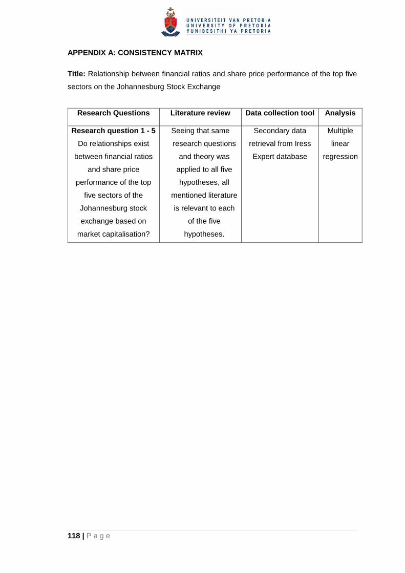
118 | P a g e
APPENDIX A: CONSISTENCY MATRIX
Title: Relationship between financial ratios and share price performance of the top five
sectors on the Johannesburg Stock Exchange
Research Questions Literature review Data collection tool Analysis
Research question 1 - 5
Do relationships exist
between financial ratios
and share price
performance of the top
five sectors of the
Johannesburg stock
exchange based on
market capitalisation?
Seeing that same
research questions
and theory was
applied to all five
hypotheses, all
mentioned literature
is relevant to each
of the five
hypotheses.
Secondary data
retrieval from Iress
Expert database
Multiple
linear
regression

119 | P a g e
APPENDIX B: STATISTICAL OUTPUTS PER HYPOTHESIS
Hypothesis 1: Mining
Please note all outputs are the final outputs after tests were rerun accept if otherwise
indicated.
1. Regression Assumptions
1.1 One independent variable is used which is measured on a continues scale.
Variable Description
Close Percentage change in closing share price from previous period
1.2 Two or more independent variables are used
No. Variable
1 Current Ratio
2 Interest Cover
3 Debt to Equity
4 Debt to Assets
5 Return on Equity
6 Return on Assets
7 Return on Capital Employed
8 Net profit margin
9 Operating profit margin
10 Total asset turnover
11 Price-earnings ratio
12 Price-to-book ratio
13 Price-to-cash-flow
14 Dividend yield
1.3 Independence of observations exists.
Durbin Watson

120 | P a g e
1.4 The dependent variable has a linear relationship with each of the independent
variables.
Final scatterplots based on stepwise regression variables identified

121 | P a g e

122 | P a g e

123 | P a g e
Partial regression plots on stepwise regression variables identified
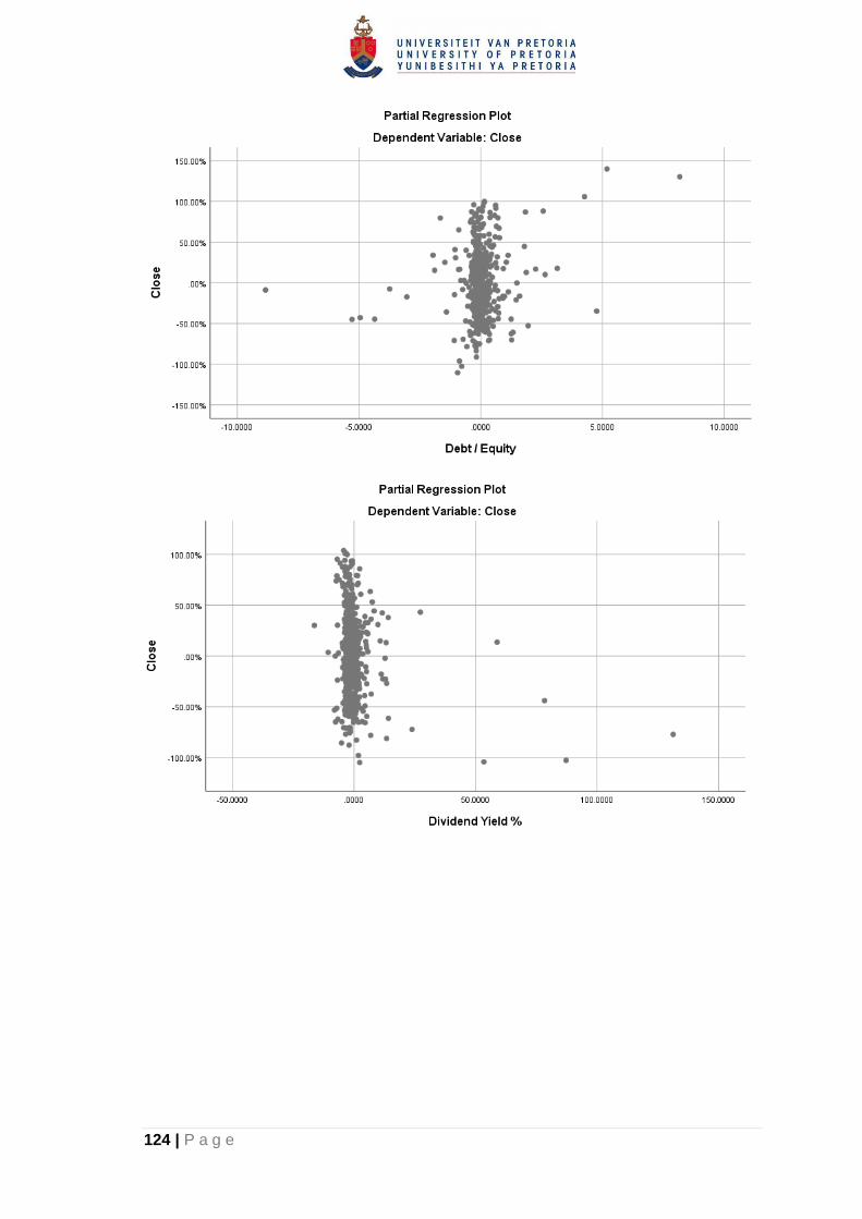
124 | P a g e

125 | P a g e

126 | P a g e
Standardized residual values versus standardized predicted values
scatterplot (With Loess curve)
1.5 The data is homoscedastic.
Standardised residual values versus the standardized predicted values
scatterplot

127 | P a g e
Koenker Test
1.6 There is no multicollinearity.
VIF and Tolerance factor
1.7 The data is free from significant outliers, highly influential points or highly leveraged
points.
Casewise Diagnostics

128 | P a g e
Round 1
Round 2
Round 3

129 | P a g e
Round 4
Round 5

130 | P a g e
Cook’s distance vs Centred leverage value (Final after removal of outliers,
highly influential and leveraged points)
1.8 The residuals (errors) are approximately normally distributed.
Histogram of regression standardized residuals

131 | P a g e
Normal P-P plot of regression standardized residual
Skewness & Kurtosis
Shapiro-Wilk

132 | P a g e
Normal Q-Q plot of Standardized Residuals
Box Plot

133 | P a g e
2. Automatic Stepwise Regression Outputs

134 | P a g e
Model 6 below is the final stepwise multiple linear regression model

135 | P a g e

136 | P a g e

137 | P a g e
Hypothesis 2: Banking
Please note all outputs are the final outputs after tests were rerun accept if otherwise
indicated.
1. Regression Assumptions
1.1 One independent variable is used which is measured on a continues scale.
Variable Description
Close Percentage change in closing share price from previous period
1.2 Two of more independent variables are used.
No. Variable
1 Current Ratio
2 Interest Cover
3 Debt to Equity
4 Debt to Assets
5 Return on Equity
6 Return on Assets
7 Return on Capital Employed
8 Price-earnings ratio
9 Price-to-book ratio
10 Price-to-cash-flow
11 Dividend yield
1.3 Independence of observations exists.
Durbin Watson

138 | P a g e
1.4 The dependent variable has a linear relationship with each of the independent
variables.
Final scatterplots based on stepwise regression variables identified

139 | P a g e
Partial regression plots on stepwise regression variables identified
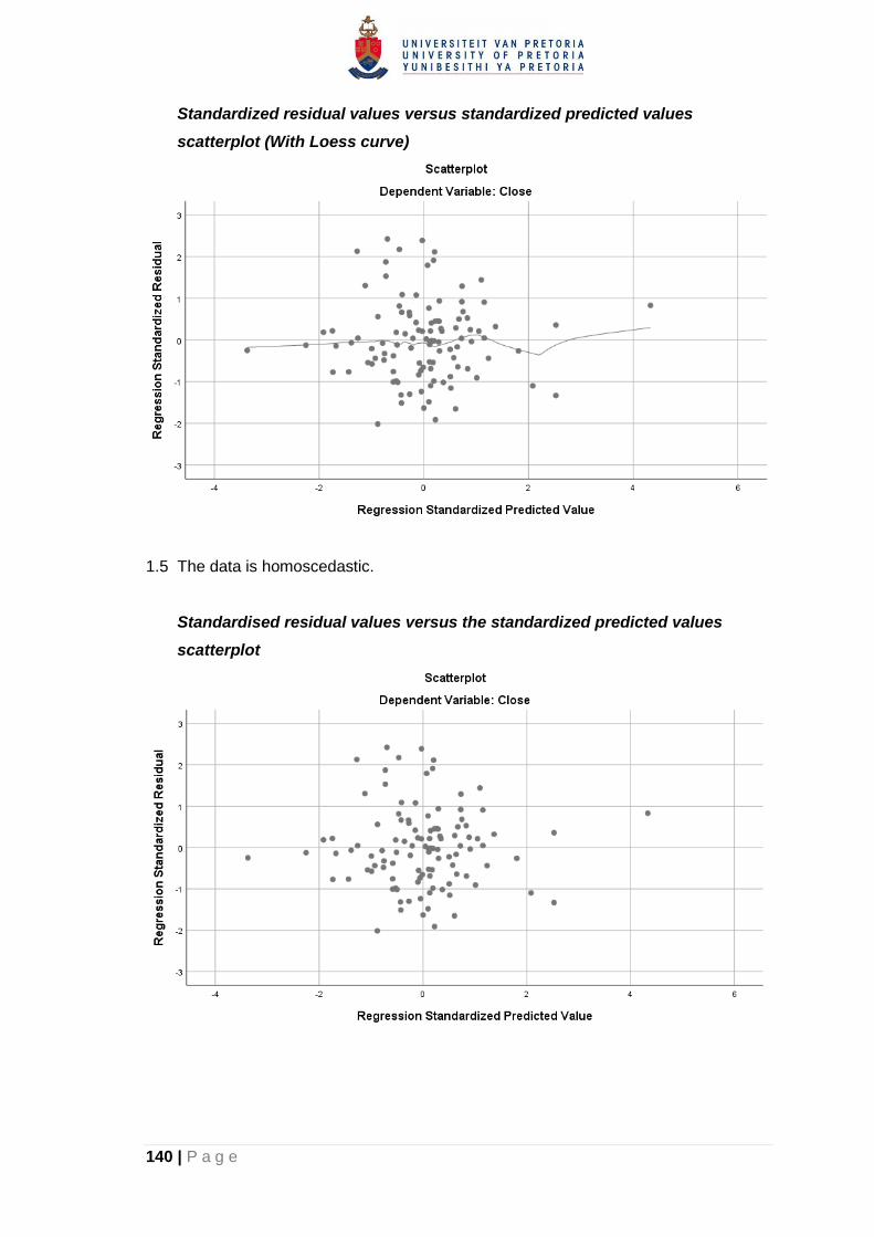
140 | P a g e
Standardized residual values versus standardized predicted values
scatterplot (With Loess curve)
1.5 The data is homoscedastic.
Standardised residual values versus the standardized predicted values
scatterplot
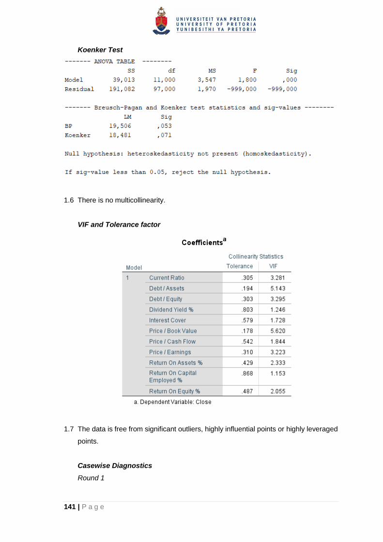
141 | P a g e
Koenker Test
1.6 There is no multicollinearity.
VIF and Tolerance factor
1.7 The data is free from significant outliers, highly influential points or highly leveraged
points.
Casewise Diagnostics
Round 1

142 | P a g e
Round 2
Round 3
Cook’s distance vs Centred leverage value (Final after removal of outliers,
highly influential and leveraged points)

143 | P a g e
1.8 The residuals (errors) are approximately normally distributed.
Histogram of regression standardized residuals
Normal P-P plot of regression standardized residual

144 | P a g e
Skewness & Kurtosis
Shapiro-Wilk
Normal Q-Q plot of Standardized Residuals

145 | P a g e
Box Plot
2. Automatic Stepwise Regression Outputs
Model 2 below is the final stepwise multiple linear regression model
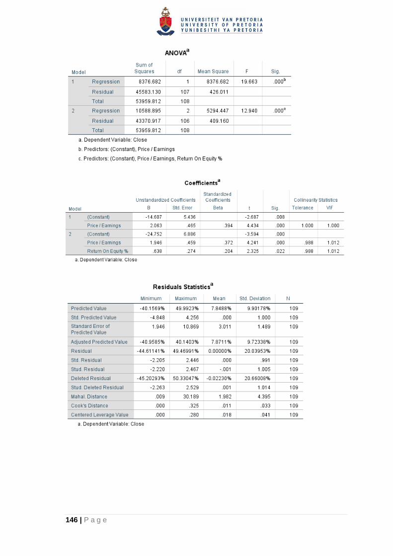
146 | P a g e

147 | P a g e
Hypothesis 3: Life Insurance
Please note all outputs are the final outputs after tests were rerun accept if otherwise
indicated.
1. Regression Assumptions
1.1 One independent variable is used which is measured on a continues scale.
Variable Description
Close Percentage change in closing share price from previous period
1.2 Two or more independent variables are used.
No. Variable
1 Current Ratio
2 Interest Cover
3 Debt to Equity
4 Debt to Assets
5 Return on Equity
6 Return on Assets
7 Return on Capital Employed
8 Net profit margin
9 Operating profit margin
10 Total asset turnover
11 Price-earnings ratio
12 Price-to-book ratio
13 Price-to-cash-flow
14 Dividend yield
1.3 Independence of observations exists.
Durbin Watson
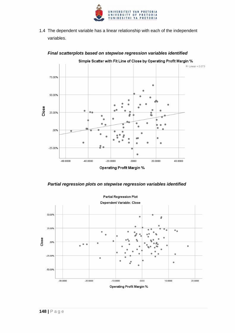
148 | P a g e
1.4 The dependent variable has a linear relationship with each of the independent
variables.
Final scatterplots based on stepwise regression variables identified
Partial regression plots on stepwise regression variables identified
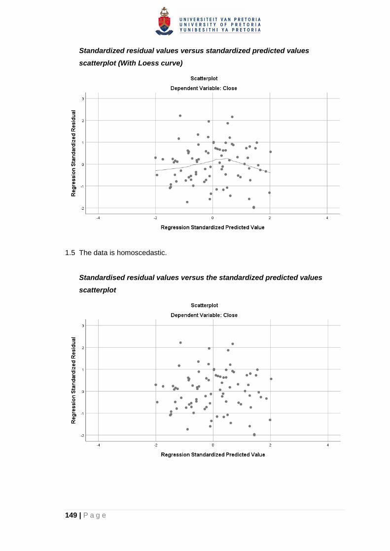
149 | P a g e
Standardized residual values versus standardized predicted values
scatterplot (With Loess curve)
1.5 The data is homoscedastic.
Standardised residual values versus the standardized predicted values
scatterplot

150 | P a g e
Koenker Test
1.6 There is no multicollinearity.
VIF and Tolerance factor
1.7 The data is free from significant outliers, highly influential points or highly leveraged
points.
Casewise Diagnostics
N/A

151 | P a g e
Cook’s distance vs Centred leverage value (Final after removal of outliers,
highly influential and leveraged points)
1.8 The residuals (errors) are approximately normally distributed.
Histogram of regression standardized residuals

152 | P a g e
Normal P-P plot of regression standardized residual
Skewness & Kurtosis
Shapiro-Wilk

153 | P a g e
Normal Q-Q plot of Standardized Residuals
Box Plot

154 | P a g e
2. Automatic Stepwise Regression Outputs
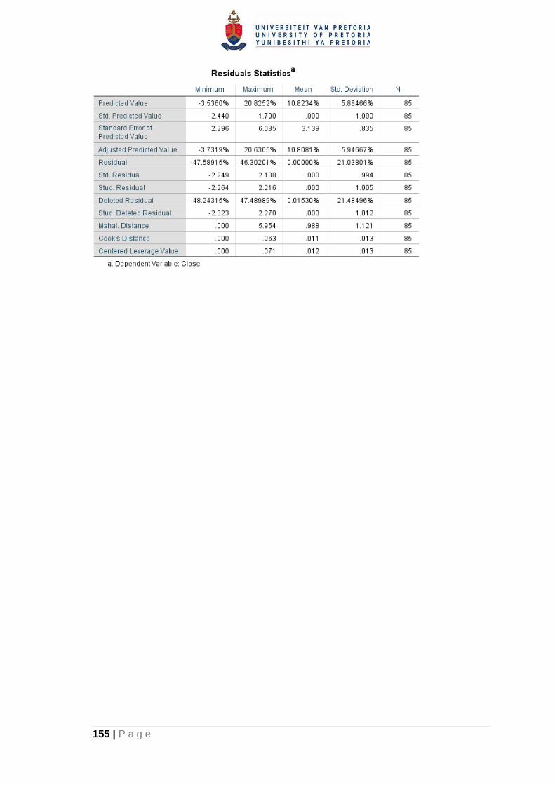
155 | P a g e

156 | P a g e
Hypothesis 4: Real Estate Investment Trusts
Please note all outputs are the final outputs after tests were rerun accept if otherwise
indicated.
1. Regression Assumptions
1.1 One independent variable is used which is measured on a continues scale.
Variable Description
Close Percentage change in closing share price from previous period
1.2 Two or more independent variables are used.
No. Variable
1 Current Ratio
2 Interest Cover
3 Debt to Equity
4 Debt to Assets
5 Return on Equity
6 Return on Assets
7 Return on Capital Employed
8 Net profit margin
9 Operating profit margin
10 Total asset turnover
11 Price-earnings ratio
12 Price-to-book ratio
13 Price-to-cash-flow
14 Dividend yield
1.3 Independence of observations exists.
Durbin Watson

157 | P a g e
1.4 The dependent variable has a linear relationship with each of the independent
variables.
Final scatterplots based on stepwise regression variables identified

158 | P a g e
Partial regression plots on stepwise regression variables identified
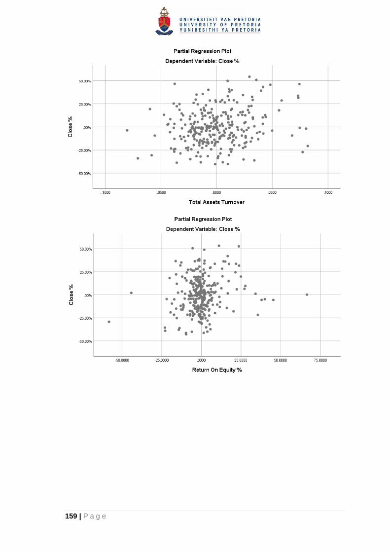
159 | P a g e
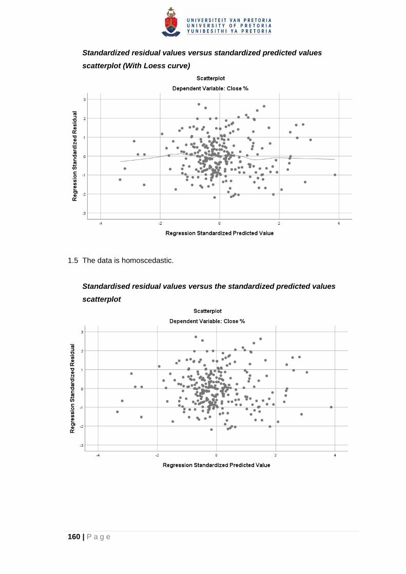
160 | P a g e
Standardized residual values versus standardized predicted values
scatterplot (With Loess curve)
1.5 The data is homoscedastic.
Standardised residual values versus the standardized predicted values
scatterplot
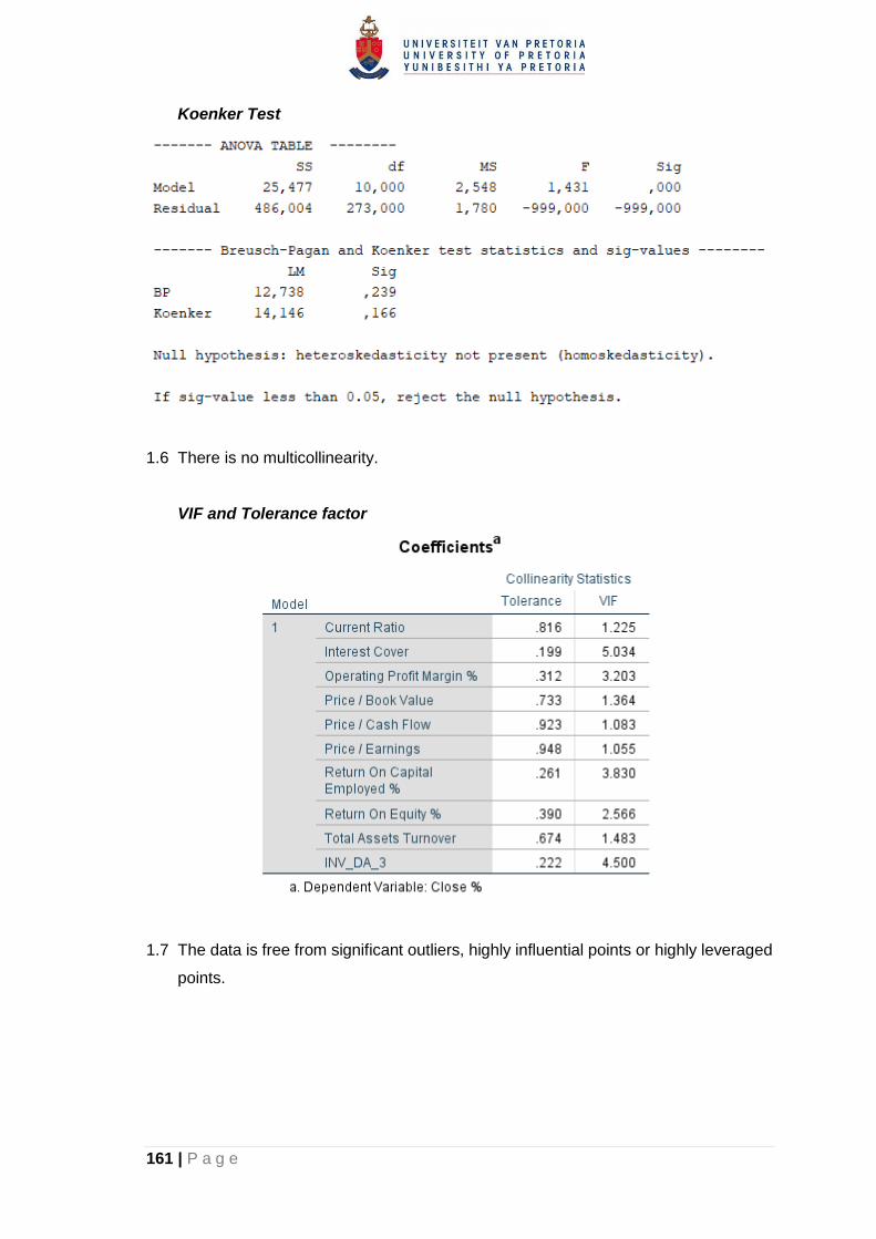
161 | P a g e
Koenker Test
1.6 There is no multicollinearity.
VIF and Tolerance factor
1.7 The data is free from significant outliers, highly influential points or highly leveraged
points.

162 | P a g e
Casewise Diagnostics
Round 1
Round 2
Cook’s distance vs Centred leverage value (Final after removal of outliers,
highly influential and leveraged points)

163 | P a g e
1.8 The residuals (errors) are approximately normally distributed.
Histogram of regression standardized residuals
Normal P-P plot of regression standardized residual

164 | P a g e
Skewness & Kurtosis
Shapiro-Wilk
Normal Q-Q plot of Standardized Residuals

165 | P a g e
Box Plot
2. Automatic Stepwise Regression Outputs

166 | P a g e
Model 3 below is the final stepwise multiple linear regression model

167 | P a g e

168 | P a g e
Hypothesis 5: Mobile Telecommunications
Please note all outputs are the final outputs after tests were rerun accept if otherwise
indicated.
1. Regression Assumptions
1.1 One independent variable is used which is measured on a continues scale.
Variable Description
Close Percentage change in closing share price from previous period
1.2 Two or more independent variables are used.
No. Variable
1 Current Ratio
2 Interest Cover
3 Debt to Equity
4 Debt to Assets
5 Return on Equity
6 Return on Assets
7 Return on Capital Employed
8 Net profit margin
9 Operating profit margin
10 Total asset turnover
11 Price-earnings ratio
12 Price-to-book ratio
13 Price-to-cash-flow
14 Dividend yield
1.3 Independence of observations exists.
Durbin Watson
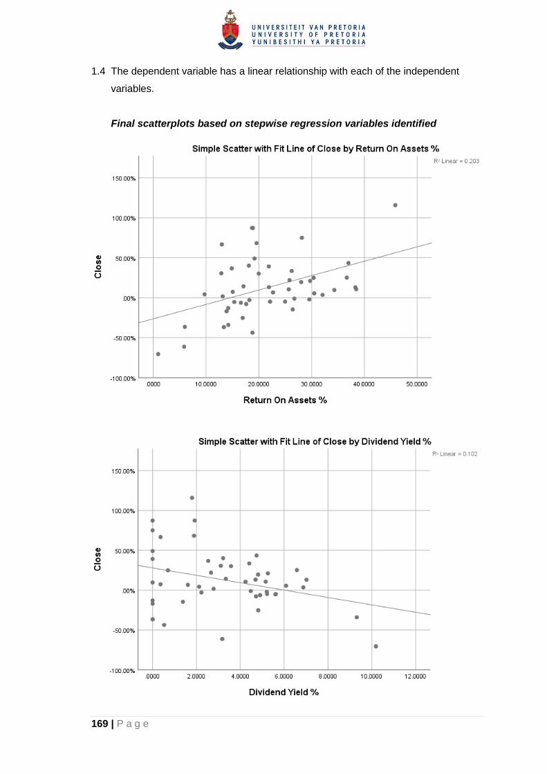
169 | P a g e
1.4 The dependent variable has a linear relationship with each of the independent
variables.
Final scatterplots based on stepwise regression variables identified
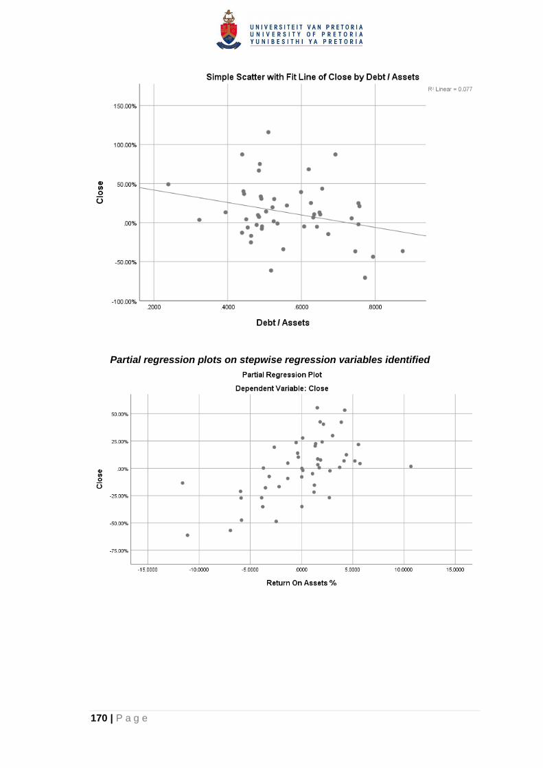
170 | P a g e
Partial regression plots on stepwise regression variables identified

171 | P a g e

172 | P a g e
Standardized residual values versus standardized predicted values
scatterplot (With Loess curve)
1.5 The data is homoscedastic.
Standardised residual values versus the standardized predicted values
scatterplot

173 | P a g e
Koenker Test
1.6 There is no multicollinearity.
VIF and Tolerance factor
1.7 The data is free from significant outliers, highly influential points or highly leveraged
points.
Casewise Diagnostics
N/A

174 | P a g e
Cook’s distance vs Centred leverage value (Final after removal of outliers,
highly influential and leveraged points)
1.8 The residuals (errors) are approximately normally distributed.
Histogram of regression standardized residuals
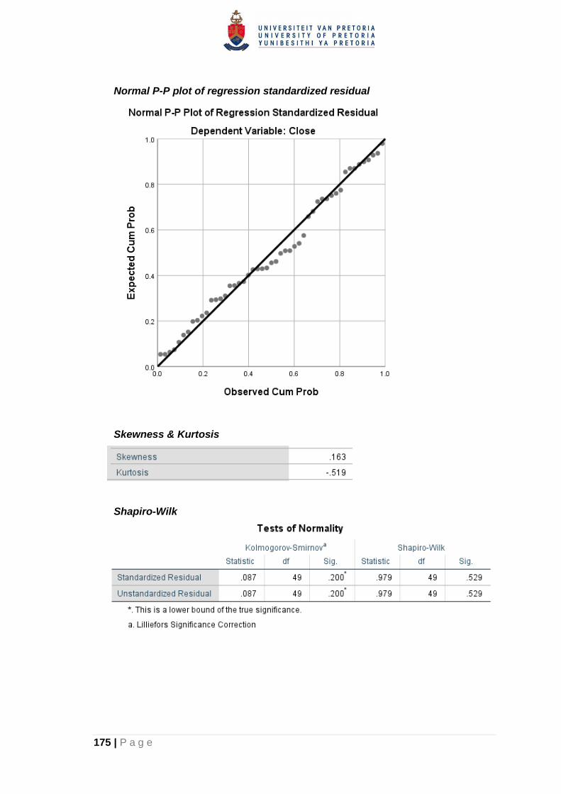
175 | P a g e
Normal P-P plot of regression standardized residual
Skewness & Kurtosis
Shapiro-Wilk
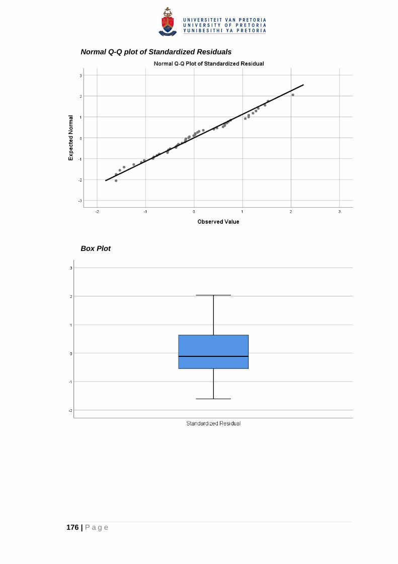
176 | P a g e
Normal Q-Q plot of Standardized Residuals
Box Plot

177 | P a g e
2. Automatic Stepwise Regression Outputs
Model 3 below is the final stepwise multiple linear regression model

178 | P a g e