Embed Size (px)
Citation preview

The relationship between share repurchase
announcement and share price behaviour
Name: P.G.J. van Erp
Submission date: 18/12/2014
Supervisor: B. Melenberg
Second reader: F. Castiglionesi

2
Master Thesis Finance
Tilburg University
Tilburg School of Economics and Management
Department of Finance
Title: The relationship between share repurchase announcement and share price behaviour
Name: P.G.J. van Erp
ANR: 600141
Supervisor: B. Melenberg
Submission date: 18/12/2014
Number of words: 15329

3
Table of Contents Chapter 1. Introduction ........................................................................................................................... 6
Chapter 2. Theory section ..................................................................................................................... 12
2.1 Shares repurchase methods ........................................................................................................ 12
2.1.1 Open market repurchases .................................................................................................... 12
2.1.2 Fixed price tender offers ...................................................................................................... 12
2.1.3 Dutch auction repurchases ................................................................................................... 12
2.2 Hypotheses .................................................................................................................................. 13
2.2.1 Mispricing hypothesis .......................................................................................................... 13
2.2.2 Free cash flows hypothesis ................................................................................................... 14
2.2.3 Earnings per share dilution hypothesis ................................................................................ 15
2.2.4 Leverage hypothesis ............................................................................................................. 16
2.2.5 Tax benefits hypothesis ........................................................................................................ 17
Chapter 3. Data analysis ........................................................................................................................ 19
3.1 Sample ......................................................................................................................................... 19
3.2 Variables ...................................................................................................................................... 23
3.2.1 Dependent variable .............................................................................................................. 23
3.2.2. Independent variables ......................................................................................................... 23
3.2.3 Control variables................................................................................................................... 25
3.3 Method ........................................................................................................................................ 26
Chapter 4. Empirical analysis ................................................................................................................. 30
4.1 Empirical results .......................................................................................................................... 30
4.1.1 The effect of the book to market ratio on the firm’s CARs .................................................. 34
4.1.2 The effect of the logarithm of total assets on the firm’s CARs ............................................ 34
4.1.3 The effect of the logarithm of market capitalization on the firm’s CARs ............................. 35
4.1.4 The effect of the total number of employees on the firm’s CARs ....................................... 35
4.1.5 The effect of the free cash flow on the firm’s CARs ............................................................. 35
4.1.6 The effect of the return on assets ratio on the firm’s CARs ................................................. 36
4.1.7 The effect of the options outstanding on the firm’s CARs ................................................... 36
4.1.8 The effect of the options exercised on the firm’s CARs ....................................................... 37
4.1.9 The effect of the debt to asset ratio on the firm’s CARs ...................................................... 37
4.1.10 The effect of the percentage of dividend on the firm’s CARs ............................................ 37
4.1.11 The effect of the dividend dummy on the firm’s CARs ...................................................... 38
4.2 Sensitivity analysis ....................................................................................................................... 45

4
Chapter 5. Conclusion and discussion ................................................................................................... 46
Literature ............................................................................................................................................... 51
Appendix ................................................................................................................................................ 54

5
Abstract
In this thesis I investigate the relationship between share repurchase announcement and share
price behaviour for the period 2000-2012, by assessing the cumulative abnormal returns
(CARs) of share repurchases. The study includes 749 unique share repurchase
announcements. I find a cumulative average abnormal return of 0.04, by investigating the
window of one day before until one day after the share repurchase announcement. Moreover,
this is statistically significant at the 1% significance level. Additionally, I find a statistically
significant positive relation between the book to market ratio and the firm’s CARs, at the 5%
significance level. I also find a statistically significant negative relation between the logarithm
of total assets and the firm’s CARs, at the 1% significance level. Furthermore, I find a
statistically significant negative relation between the logarithm of market capitalization and
the firm’s CARs, at the 1% significance level. All three of these results are consistent with the
mispricing hypothesis. Additionally, I find a statistically significant negative relation between
dividend paying firms and the firm’s CARs, at the 10% significance level. This is consistent
with the tax benefits hypothesis. Also the hypotheses: free cash flow hypothesis, earnings per
share dilution hypothesis, and the leverage hypothesis, are tested. The free cash flow and the
return on assets are used to test the free cash flow hypothesis. I find mixed results between the
relations of these variables on the firm’s CARs. But none of these results are significant. For
the relation between the options outstanding and options exercised with the firm’s CARs, a
positive insignificant relation is found. So, no evidence is found to support the earnings per
share dilution hypothesis. Finally, I find a positive relation between debt to asset ratio and the
firm’s CARs. This is consistent with the theory for the leverage hypothesis. However this
result is not statistically significant.

6
Chapter 1. Introduction
Share repurchase programs have been increasingly popular over the last years and are also
gaining importance. One of the explanations for the increasing popularity of share repurchase
behaviour is the change in governance over the last years. Brav et al. (2005) conclude that
share repurchases are now a more important form of payout compared to the past. This
upward trend of popularity for share repurchases already started in the 1980s. Since then there
are multiple studies conducted about the short- and long-term effects of share repurchases.
Most of the considered ‘relevant papers’, such as Vermaelen (1981), Ikenberry et al. (1995),
Stephens and Weisbach (1998), and Lie (2005), find positive cumulative abnormal return
(CAR) for the short- and long term horizon around the announcement date. But, this is not the
case for all studies, for example Grullon and Michaely (2004) find that repurchase
announcements are not followed by an increase in performance. Additionally, there is a
debate about many of the explanations and consequences of the effect share repurchase
announcements have on share price behaviour. Moreover, mixed results are found about these
explanations in the literature. In this study I try to tackle this problem by investigating the
possible effects share repurchase announcements have on share price behaviour. I do this by
first investigating the relation between share repurchase announcements and share price
behaviour. Next, to investigate the possible reasons for the effect share repurchase
announcements have on share price behaviour, I come up with five hypothesis based on past
literature. These hypotheses are the mispricing hypothesis, free cash flow hypothesis, earnings
per share dilution hypothesis, leverage hypothesis, and tax benefits hypothesis. These
hypotheses have already been tested collectively in the literature, or in some papers only one
or more of these hypothesis are tested. In this study I explain the effects that multiple
variables could have on the firm’s CARs. Furthermore, this study is conducted over a
relatively recent period of 2000 until 2012
The mispricing hypothesis is based upon signalling undervaluation of a company. Assuming
the market is imperfect, because there is asymmetric information between insiders (typically
the managers) and outside investors. The asymmetry could lead to mispricing of companies.
Vermaelen (1981, 1984) concludes that firms offer premia for their shares, mainly in order to
signal positive information. Also Dann (1981) concludes that firm values significantly
increase within one day of a common stock repurchase announcement, principally due to the
signalling of information. Stephens and Weisbach (1998) support the mispricing hypothesis

7
by finding a negative relation between share repurchases and prior stock performance,
suggesting that firms increase their purchasing depending on their degree of perceived
undervaluation. In addition, also Dittmar (2000) finds evidence that supports the
undervaluation hypothesis. However, in contrast to the studies discussed before, Chan et al.
(2004) and Jagannathan and Stephens (2003) show only modest evidence for the mispricing
hypothesis. Dittmar and Dittmar (2008) even show evidence against it, by analyzing waves in
corporate finance events including stock repurchases.
The free cash flow hypothesis is based on the separation of ownership and control in
companies, because this separation could possibly lead to agency costs. By repurchasing
shares, the managers could be more constrained, because it reduces the excess free cash flow.
For example, by reducing the free cash flows there is less room for investing in negative net
present value projects. The free cash flow hypothesis is supported by Stephens and Weisbach
(1998). Also, Gangopadhyay et al. (2010), and Grullon and Michaely (2004) support the free
cash flow hypothesis. They find that firms with free cash flows earn significantly higher
abnormal returns than all other firms. Finally, Chan et al. (2004) find limited support for the
free cash flow hypothesis.
The earnings per share (EPS) dilution hypothesis is based on the tendency that managers often
try to manage measurements such as the EPS. Moreover, one of the reasons to repurchase
stocks could be to prevent EPS dilution, because of the simple principle that the reduction of
common shares outstanding leads to an increase in the value per share, since the company’s
value is shared by less investors. Kahle (2002) provides evidence to support the earnings per
share dilution hypothesis. Also Bens et al. (2003) show support for the prevention of the EPS
dilution by firms, by repurchasing shares. Moreover, Brav et al. (2005) conclude that firms
are likely to repurchase shares when their stock’s float is adequate, and when Chief Financial
Officers (CFOs) have the desire to offset option dilution. Additionally, they find that two-
thirds of their survey respondents feel that offsetting dilution is an important or very
important factor affecting their repurchase decisions.
The leverage hypothesis is based on the adjustment of the capital structure. By repurchasing
shares, firms could adjust their capital structure to look for a more beneficial leverage ratio.
Modigliani and Miller (1958, 1963) opened the discussion in scientific research about
adjusting the capital structure in order to find a more optimal leverage ratio. This theory is
mainly based on the effect of tax benefits of interest payments by adjusting the firm’s capital

8
structure. Dittmar (2000) and Hovakimian et al. (2001) provide evidence to support the
leverage hypothesis. On the other hand, Chan et al. (2004) do not find enough evidence to
support the leverage hypothesis.
Finally, the tax benefits hypothesis is based on the difference in tax burdens. For example,
share repurchases could be more beneficial to shareholders than dividends. Black (1976)
states that a corporation that pays no dividends will be more attractive to taxable individual
investors than a similar corporation that pays dividends, when dividends are taxed more
heavily than capital gains, and where capital gains are not taxed until realized. Grullon and
Michaely (2002) state that it is more efficient to return capital to shareholders through a stock
repurchase program instead of dividends after the reduction in long-term capital gains tax.
However, Jagannathan et al (2000) do not find evidence to support this conclusion. Moreover,
Brav et al. (2005) conducted a survey about the payout behaviour of managers. They find that
managers at most firms do believe that taxes are not a dominant factor that affects the payout
decision making.
The method used in my master thesis to measure share price behaviour is an event study.
First, the abnormal returns are calculated. This is used to measure the economic impact of
share repurchases, over a relatively short period of time. By subtracting the firm’s predicted
‘normal returns’ from the firm’s actual returns, the abnormal returns are calculated. The
predicted ‘normal returns’ are calculated by using an estimation window that is considered not
to be affected by the announcement of share repurchases. The main event windows used in
this study are: one day before until one day after the announcement of share repurchase [-1,1],
and ten days before until 2 days before the announcement of share repurchase [-10,-2]. The
estimation window is 200 days before until 31 days before the announcement of share
repurchase [-200,-31]. Furthermore, to evaluate the effect of share repurchase announcements
on share price behaviour, more event windows are used. In total nine event windows are used:
[-1,1], [-3,3], [-1,1], [-5,1], [-5,5], [-10,-2], [-10,10], [-15,1], [-15,15], [-30,30], these indicate
days around the announcement day of share repurchase at day 0. To calculate the abnormal
returns, the market model is used, opposed to the related Capital Asset Pricing Model
(CAPM), and the Arbitrage Pricing Theory (APT). This is further explained in chapter 3.3. As
explained by MacKinlay (1997), the market model is a statistical model which relates the
return of any given security to the return of the market portfolio.

9
In this study I obtained a sample that consists of companies from the United States. They are
listed on the indices: NASDAQ, NYSE and AMEX. The sample includes 1087 share
repurchase announcements with unique companies, and it only includes open market
repurchases. In order to create a sample where all variables have the same number of
observations, 749 firms from the full sample are selected. Firms from the divisions Finance,
Real Estate, and Insurance are excluded from the study. Also, firms from the division
Communications, Electric, Gas and Sanitary service, and Transportation, are excluded from
the study. The reason for this is that it is more likely that these firms were regulated. To
obtain my data, the Center for Research in Securities Pricing (CRSP) database, the Securities
Data Corporation (SDC) database, and COMPUSTAT are used.
In order to test the mispricing hypothesis, the free cash flow hypothesis, the earnings per share
dilution hypothesis, the leverage hypothesis, and the tax benefits hypothesis, a time series
ordinary least squares (OLS) regression is used. To test the five hypothesis further explained
in chapter 2.2, several variables are used, further explained in chapter 3.2. Each of the
independent variables is used to test for one of the five hypotheses. Most variables are based
on past literature, such as Bens et al (2003), Ikenberry et al. (1995), Grullon and Michaely
(2002, 2004) and Lie (2005). To test for the mispricing hypothesis, I added the number of
employees as a proxy for size.
In my study I investigate the effect share repurchase announcements have on share price
behaviour. This study is conducted for several windows around the announcement day. Based
on the window [-1,1] I find a cumulative average abnormal return (CAAR) of 0.04, this is
statistically significant1 at the 1% significance level. So, share repurchase has a significant
positive effect on share price behaviour. Besides, the window [-10,-2] is used to test the
relation between share repurchase and prior stock performance. The corresponding CAAR is
-0.07 and it is statistically significant, at the 5% significance level. This provides evidence for
the mispricing hypothesis. Furthermore, I find a positive statistically significant relation
between the book to market ratio and the firm’s CARs, at the 5% significance level. I also
find a negative statistically significant relation between the logarithm of market capitalization
and the firm’s CARs, and also for the relation between the logarithm of total assets and the
firm’s CARs, both at the 1% significant level. All these results show support for the 1 The default level for statistical significance throughout the rest of this study is set to a 10% statistical significance level. So, with statistical significance I mean the statistical significance at a 10% level. If the statistical significance level is different, this is mentioned explicitly.

10
mispricing hypothesis. Furthermore, I find a negative relation between the number of
employees and the firm’s CARs. However, this is not statistically significant.
To investigate for the free cash flow hypothesis, I tested the effects of free cash flow and
return on assets on the firm’s CARs. For both variables I find mixed results about the relation
with the firm’s CARs. But none of these results are statistically significant.
To investigate for the earnings per share dilution hypothesis, I tested the effects of options
outstanding and the options exercised on the firm’s CARs. I predicted it to have a negative
relation with the firm’s CARs. However, for both variables I find a positive relation between
the independent variable and the firm’s CARs. But these relations are not statistically
significant.
To investigate for the leverage hypothesis, I tested the effect of debt to assets ratio on the
firm’s CARs. I predicted it to have a positive relation between the debt to assets ratio and the
firm’s CARs. I indeed find a positive relation between these variables, but this relation is not
statistically significant.
Finally, to investigate the tax benefits hypothesis, I tested the effects of dividend dummy and
percentage of dividend on the firm’s CARs. For both of these relations I predicted it to have a
negative relation with firm’s CARs. I also find a negative statistically significant relation
between dividend dummy and the firm’s CARs. On the other hand, I find a positive
statistically significant relation between percentage of dividend and the firm’s CARs.
However, this last result is based on a regression which has some levels of multicollinearity.
This is explained in chapter 4.1. So, this last result is treated with caution.
To conclude, my results show support for the mispricing hypothesis and the tax benefits
hypothesis. Based on the other results, I do not provide enough evidence to support the free
cash flow hypothesis, earnings per share dilution hypothesis, and the leverage hypothesis.
I also provide evidence for different abnormal returns because of share repurchases among
different industries. This might be interesting to investigate as part of future research. Another
recommendation for future research is to try combining other data sources such as Zephyr,
Orbis, or firm’s financial reports, to obtain a full sample without performing a selection
process. Besides, it would be interesting to also test for the long term effect of share
repurchases. Furthermore, the agency costs theory, explained in chapter 2.1, could be
investigated more specifically. I found evidence for the mispricing hypothesis, which is
11
related with agency costs, but it is for example interesting how this would relate to manager’s
compensation and ownership.
The structure to explain the sample analysis, method, and empirical results shows similarities
with my previous conducted master thesis, van Erp (2014). Moreover, the description of the
dependent variable and the description of the variable industry dummy are also similar to the
descriptions provided in this master thesis.
The remainder of my master thesis is organized as follows: Chapter 2 presents the theory
section. Chapter 3 presents the data analysis, it describes the sample, variables, and the
method used in this study. Chapter 4 presents the empirical analysis, it consists of the
empirical results and a sensitivity analysis. Chapter 5 presents the conclusion and discussion.

12
Chapter 2. Theory section
2.1 Shares repurchase methods Repurchasing Shares of its own company became increasingly popular over the last years and
are also gaining importance When repurchasing its own shares, a company distribute a large
amount of money to its shareholders. There are several methods to repurchase the shares, the
most essential methods are: open-market, fixed price tender offer, and Dutch auction tender
offer. These three methods are explained below.
2.1.1 Open market repurchases
Among the three methods, the open market repurchase is the most popular. Chan et al. (2004)
report a big increase in the number of firms announcing open market stock repurchases in the
1990s. In an open market repurchase, the firm announces to repurchase their stock on the
open market. So, the repurchase price of the stock will be based on the market price, and is
just the same as for any other investor.
2.1.2 Fixed price tender offers
In fixed price tender offers the share price, number of shares, and duration of the offer is
predefined. In contrast to open market repurchases these conditions are fixed. When issuing
fixed price tender offers the firm gives shareholders the option to tender within the predefined
condition. Additionally, the firm can set a target to the minimum number of tendered shares.
If this condition is not met it still has the option to repeal the offers. Moreover, the firm is also
allowed to adjust the duration of the period for repurchase and it could change the number of
shares it want, to repurchase.
2.1.3 Dutch auction repurchases
The Dutch auction was a specification of the fixed price tender method, introduced in 1981.
Dutch auction repurchases are somewhat similar to fixed price tender offers, except for Dutch
auction repurchases the firm offers a range of prices shareholders can sign up to. Shareholders
can tender for the minimum price of a specified number of shares they are willing to accept.
The firm can repeal the offers when there are fewer shares submitted for sale as the
predefined amount, or it can repurchase the shares at the tendered prices. When there are more
shares submitted for sale, the firm repurchases shares at a uniform lowest price possible that
allows them to buy back the predetermined number of shares. So, this price is offered to
shareholders who tendered at or below this price.

13
2.2 Hypotheses
In this section I elaborate on the possible explanations why firms repurchase shares.
Furthermore, I come up with different hypotheses about the relation between share
repurchases and firm performance.
2.2.1 Mispricing hypothesis
The mispricing hypothesis is based upon signalling for undervaluation of a company.
Assuming the market is imperfect, because there is asymmetric information between insiders
(typically the managers) and outside investors. The asymmetry could lead to mispricing of
companies. Following the reasoning provided by Erken (2012), In most cases the managers
are better informed about the current and future prospects of the company. For example, about
the company’s expectations, its opportunities, and prospects. When the corporation is
undervalued, so the company is actually worth more than the current market value, managers
could have the incentive to adjust this mispricing. To make the statement of undervaluation
believable, the managers could repurchase their own stock to signal a positive view about the
future of the corporation. Eventually, this could lead to a positive stock price reaction. Often
in the literature a distinction is made between value stocks and growth stocks. Firms with a
high book to market ratio are considered to have value stocks, and firms with a low book to
market ratio are considered to have growth stocks. As concluded by Ikenberry, Lakonishok,
and Vermaelen (1995), value stocks are more likely to have undervaluation as their primary
motivation. Vermaelen (1981, 1984) concludes that firms offer premia for their shares, mainly
in order to signal positive information. It also makes a distinction between small firms and
large firms. Small firms are considered to have higher levels of information asymmetry. Also
Dann (1981) concludes that firm values significantly increase within one day of a common
stock repurchase announcement. These increases principally appear to be due to an
information signal from the repurchasing firm. As stated by Dann (1981), these positive
values are considered to be permanent in a way that the share prices do not return to their pre-
announcement date levels following expiration of the opportunity for stockholder to tender
shares. However, the nature of the new information that results in a positive stock price
change is still unidentified. Stephens and Weisbach (1998) support the mispricing hypothesis
by finding a negative relation between share repurchases and prior stock performance,
suggesting that firms increase their purchasing depending on their degree of perceived
undervaluation. In addition, also Dittmar (2000) finds evidence that supports the
undervaluation hypothesis. However, in contrast to the studies discussed before, Chan et al.
14
(2004) show only modest support for the mispricing hypothesis, when testing for the short-
horizon market reaction to the share repurchase announcement. Moreover, over a four-year
window after the announcement, earnings surprises tend to be positive and significant. This
result suggests that the market does not completely incorporate the information in share
repurchase announcements. Also, the study of Jagannathan and Stephens (2003) causes
doubts for the undervaluation hypothesis. They examine differences in firms that repurchase
shares frequently versus firms that repurchase only occasionally or infrequently. They find
that frequent repurchasers may be using it as a substitute for increasing dividends, but
unlikely because of firm undervaluation. On the other hand, they find that infrequent
repurchases may be motivated by undervaluation. Still, they find a positive market reaction
for all repurchase announcements on average, but the infrequent repurchases have a much
stronger positive reaction. Finally, Dittmar and Dittmar (2008) find evidence against the
mispricing hypothesis, by analyzing waves in corporate finance events including stock
repurchases, leading to a conclusion that equity issuance (and repurchases) predicts lower
returns and likely reflects time-varying costs of capital rather than mispricing. So, to
conclude, firms could use share repurchase to adjust for the undervaluation of their company.
2.2.2 Free cash flows hypothesis
A general believe in finance is that the separation of ownership and control in companies can
lead to agency costs. By repurchasing the shares of your own companies, the managers could
be more constrained, because it reduces the excess free cash flow. As argued by Jensen (1986)
followed upon Rozeff (1982) and Easterbrook (1984)
“ Payouts to shareholders reduce the resources under managers' control, thereby reducing managers'
power, and making it more likely they will incur the monitoring of the capital markets which occurs
when the firm must obtain new capital”.
Stephens and Weisbach (1998) conducted a study including the relation between cash flow
and share repurchases. They find that both expected and unexpected cash flows are positively
related to repurchases, therefore, suggesting that firms actively adjust their share repurchases
behaviour to their cash position. Furthermore, Gangopadhyay et al. (2010) test the free cash
flow hypothesis by examining the announcement-period abnormal returns of repurchasing
firms sorted by their available investment opportunities, as measured by Tobin’s q ratio and
cash flows. They find that firms with free cash flows earn significantly higher abnormal
returns than all other firms. By reducing the free cash flows there is less room for investing in
negative net present value projects. By repurchasing stock, shareholders can invest in other

15
positive investment opportunities. In general, this could lead to a more optimal capital market
allocation, because capital is moved from negative net present value investments, towards
positive net present value investments, as argued by Grullon and Ikenberry (2000).
Eventually, it would be more beneficial for firms with a high level of free cash flow to
repurchase stock. This is supported by Grullon and Michaely (2004), who find that the market
reaction to share repurchase announcements is more positive among those firms that have
higher levels of free cash flows, and therefore were more likely to overinvest. So, by
repurchasing stock, the corporation reduces the risk of investing disproportionally. This is one
of the possible solutions to reduce empire building, because it prevents managers to focus too
much on increasing the size of the corporation, rather than the size of its profits. Furthermore,
reducing the free cash flow could reduce the fringe benefit consumption. It also could prevent
managers for holding on to underperforming subordinates for too long. However, Chan et al.
(2004) find limited support for the free cash flow hypothesis. They support the hypothesis by
showing that repurchase firms tend to have above-average free cash flow compared to their
industry peers. Moreover, the long-run drift is greater for high free cash flows firms compared
to low free cash flow cases. But, on the other hand, they can’t support the hypothesis that the
gains from high free cash flow firms should be linked to cases where managers actually
disgorge cash. So, to conclude, managers could use share repurchase to reduce agency costs.
2.2.3 Earnings per share dilution hypothesis
Earnings per share (EPS) is an important measure to analyse firms in general. Often managers
try to improve measurements such as the EPS. Moreover, one of the reasons to repurchase
stocks could be to prevent EPS dilution, because of the simple principle that the reduction of
common shares outstanding leads to an increase in the value per share, since the company’s
value is shared by less investors. Stock dilution could emerge from the issue of additional
shares. This could occur from primary market offerings, preferred shares or warrants into
stock, exercised stock options, or by conversed convertible bonds. According to Kahle (2002),
firms announce for share repurchases when executives have large numbers of options
outstanding and when employees have large numbers of options currently exercisable.
Moreover, there is a positive relation between the amount repurchased and the total options
exercisable by all employees, once the repurchase decision is made. However, the amount
repurchased is independent of managerial options according to Kahle (2002). Also Bens et al.
(2003) show support for the prevention of the EPS dilution by firms, because they find an
increase in the level of stock repurchases when the dilutive effect of outstanding employee

16
stock options on diluted EPS increases. This increase also occurs when the firm’s earnings are
lower than required to achieve their EPS growth target. This increase is based on the incentive
to manage EPS dilution, instead of also the incentive to adjust the basic EPS, according to
Bens et al. (2003). Consistent with this theory, Brav et al. (2005) find that Chief Financial
Officers (CFOs) are very conscious of the affect share repurchases have on the earnings per
share. Furthermore, they conclude that firms are likely to repurchase when their stock’s float
is adequate, and when CFOs have the desire to offset option dilution. Additionally, they find
that two-thirds of their survey respondents feel that offsetting dilution is an important or very
important factor affecting their repurchase decisions. So, share repurchase could be used to
adjust for possible share dilution.
2.2.4 Leverage hypothesis
By repurchasing shares, the corporation could adjust their capital structure, especially if the
amount of repurchases is high. This could lead to a more beneficial leverage ratio. Modigliani
and Miller (1958, 1963) opened the discussion in scientific research about adjusting the
capital structure in order to find a more optimal leverage ratio. This theory is mainly based on
the effect of tax benefits of interest payments by adjusting the firm’s capital structure. So, by
repurchasing stocks, firms are able to adjust their leverage ratio. According to Dittmar (2000),
this is one of the reasons why firms repurchase stocks during certain periods. Hovakimian et
al. (2001) continue on the theory that firms adjust their capital structure, to move to a target
debt ratio. They take a closer look at the impediments firms may face when moving toward
their target ratio, and the possible change in the target ratio over time. To conclude, they find
that capital structure considerations are more important for firms when they repurchase stock
rather than raise capital. Moreover, Hovakimian et al. (2001) state
“The tendency of firms to make financial choices that move them toward a target debt ratio appears
to be more important when they choose between equity repurchases and debt retirements than when
they choose between equity and debt issuances.”
However, Chan et al. (2004) do not support the leverage hypothesis, although they find that
repurchasing firms tend to have below average leverage, but these firms do not have any
higher drift when compared to firms with a higher leverage. Also, there was no significant
distinction in returns for firms that had sharp declines in leverage. Also, Brav et al. (2005)
find little support for the leverage hypothesis by surveying financial executives and
conducting in-depth interviews. So, to conclude, firms could repurchase share to adjust their
capital structure to reach for a more optimal capital structure.

17
2.2.5 Tax benefits hypothesis
There are several ways of returning profits or an excess of capital to the shareholders. For
example, share repurchases could be more beneficial to shareholders than dividends, because
of tax benefits. So, the difference in tax burden could be a reason for companies to repurchase
shares. Black (1976) states that a corporation that pays no dividends will be more attractive to
taxable individual investors than a similar corporation that pays dividends, when dividends
are taxed more heavily than capital gains, and where capital gains are not taxed until realized.
The tax benefits of share repurchases in the US were especially beneficial before the For Jobs
and Growth Tax Relief Reconciliation Act of 2003, because of the much lower taxation on
capital gains versus dividend payments. After the Jobs and Growth Tax Relief Reconciliation
Act of 2003, the taxes on qualified dividends 2were lowered to the capital gains level. This
was set to expire after 2010. However, in the Tax Relief, Unemployment Insurance
Reauthorization, and Job Creation Act of 2010 the dividends and capital gains rates were
extended for another two years. Finally, in the American Taxpayer Relief Act of 2012, the tax
rate levels on capital gains and dividends for 2013 remained the same as in 2012 for
individuals with taxable income of $400,000 per year or less. For individuals with taxable
income over $400,000, the top marginal tax rate on long-term capital gains was set to the
level of 20% for under expiration of the Jobs and Growth Tax Relief Reconciliation Act of
2003. The top marginal tax rate on dividends remained at the similar level as capital gains, so
also 20%, instead of the much higher 39,6% rate under expiration of the Jobs and Growth Tax
Relief Reconciliation Act of 2003. But after these changes in tax rates, share repurchases are
still considerate to be more beneficial than dividends, because investors have the option to
defer capital gains or losses by holding on to their shares. On the other hand, dividends are
taxed immediately when received. Blouin et al. (2007) tests for policy changes in dividends
and repurchases following the Jobs and Growth Tax Relief Reconciliation Act of 2003. They
find evidence consistent with dividends crowding out repurchases, as a result of reductions in
dividends and capital gains tax rates. However, Grullon and Michaely (2002) state that it is
more efficient to return capital to shareholders through a stock repurchase program instead of
dividends after the reduction in long-term capital gains tax. Moreover, they show that there is
a more positive market reaction to repurchases when the tax gains from repurchases relative
to dividends are larger. On the other hand, Jagannathan et al (2000) do not find evidence to
2 For a description of qualified dividends, see
http://www.irs.gov/instructions/i1099div/ar02.html#d0e154

18
support this conclusion. Their work suggests that besides taxes much more is necessary to
explain differences in motives to use dividends and repurchases. As discussed earlier, Brav et
al. (2005) conducted a survey about the payout behaviour of managers. They find that
managers at most firms do believe that taxes are not a dominant factor that affects the payout
decision making. Moreover, they state that executives believe that repurchases and dividends
are equally attractive to most institutional investors. So in general, share repurchase could be
used to return profits or an excess of capital to shareholders in a more tax beneficial way for
the shareholders.

19
Chapter 3. Data analysis
In order to analyze my data I will first describe the sample. Next, the variables will be
analyzed. Finally, the method I use in this study will be explained. This is the same order to
analyze data as used in van Erp (2014).
3.1 Sample In this study I obtained a sample that consists of companies from the United States. They are
listed on the indices: NASDAQ, NYSE and AMEX. 498 of the companies are listed in the
NYSE index, 552 in the NASDAQ index, and 37 in the AMEX index. The sample includes
share repurchase announcements for the period 2000-2012. It only includes open market
repurchases. Firms from the divisions Finance, Real Estate, and Insurance are excluded from
the study. These are marked by the Standard Industrial Classification (SIC) codes 6000 until
6799. Also, firms from the division Communications, Electric, Gas and Sanitary service,
Transportation, marked by the SIC codes 4000 until 4999, are excluded from the study. The
reason for this is that it is more likely that these firms were regulated. In total 505 firms were
removed from the sample because of this. Eventually, I end up with a sample consisting of
1087 share repurchase announcements with unique companies. The statistics about the
variables used in this study are listed in table 1. To obtain my data, the Center for Research in
Securities Pricing (CRSP) database, the Securities Data Corporation (SDC) database, and
COMPUSTAT are used.
As displayed in table 1 not all the variables have the same number of observations, this is
because of missing data for some firms. In order to conduct my study, I created a sample
where all variables have the same number of observations. This is displayed in table 2.
Because of this selection, a selection bias might occur. Moreover, t-tests are conducted to test
for differences in means among table 1 and 2. In the tables A13 and A14, the dependent
variables CAR[-1,1] and CAR[-10,-2] are tested respectively. In these t-tests the 𝐻0
hypothesis is that the mean CAR of table 1 and the mean CAR of table 2 are equal. So, the
difference between the two variables is zero. The alternative hypothesis is: the difference
between the mean CAR of table 1 and the mean CAR of table 2 is unequal to zero. Based on
both tables the 𝐻0 hypothesis: the mean CAR of table 1 and the mean CAR of table 2 are
equal, cannot be rejected, because the corresponding p-values are 0.3901 and 0.9681 in tables
A13 and A14 respectively. So, there is no evidence found that the two samples are different.

20
Furthermore, for each independent variable a similar t-test is conducted. For all of the
variables except for the options outstanding, the 𝐻0 hypothesis: the mean of the variable in
table 1 and the mean of the variable in table 2 are equal, cannot be rejected. In table A15 the t-
test for the options outstanding is displayed. Based on the p-value of 0.0939, the 𝐻0
hypothesis can be rejected, at the 10% significance level. But, based on all the t-tests I
conclude that there does not seem to be any level of selection bias, and that the sample
displayed in table 2 is still representative of the population that I intend to analyse. Moreover,
by conducting a t-test for all the 17 variables separately, at the 10% significance level, I could
expect that 10% of the test results will be rejected.

21
Table 1
Descriptive statistics of the full sample
This table provides the descriptive statistics of the full sample over the period 2000-2012. It provides the statistics about the number of observations, mean, standard deviation, and the minimum and maximum value of the variables. The currency in the descriptive statistics is the U.S. dollar. The ‘MM’ behind some variables stands for measured in millions. The cumulative abnormal return (CAR) [-1,1] is based on the window 1 day before the announcement of share repurchase until 1 day after the announcement of share repurchase. The window [-10,-2], stands for 10 days before the announcement of share repurchase until 2 days before the announcement. The book to market ratio is calculated by dividing the book value of equity by the market value of equity. The market capitalization is calculated by multiplying the share price with the number of common shares outstanding. The free cash flow is calculated by dividing the variable ‘Cash’ by the book value of equity. The capital expenditure is used as a percentage of the total assets. The return on assets is calculated by dividing net income by total assets. Options outstanding represent the stock options that are exchangeable for common stock of the firm. Options exercised represent the total number of stock options that were exercised for common stock. Debt to asset ratio is calculated by dividing long term debt by total assets. Total dividend ratio is calculated by dividing total dividend by total assets. Dividend dummy is a variable about the distinction between firms that pay dividends and firms that do not pay dividend. Firms that pay dividend are marked by ‘1’ and firms that do not pay dividend are marked by ‘0’. Finally, three industry dummies are displayed. Each of the dummies takes on the value 1 if the firm is from that particular industry.
Variable Observations Mean Std. Dev. Min Max
CAR [-1.1] 1087 0.04 0.34 -5.03 2.45
CAR [-10.-2] 1087 -0.07 0.97 -16.43 5.14
Book to market ratio 1081 0.59 0.51 0.00 7.16
Logaritm of total assets 1084 6.65 1.83 -3.41 13.53
Logaritm of market capitalization 1082 6.76 1.97 -4.89 12.86
Number of employees 1071 15450.39 58385.41 4 1383000
Free cash flow 1074 0.36 1.45 0 35.38
Percentage of capital expenditures 1078 0.05 0.06 0 0.55
Return on Assets 1084 0.04 0.25 -5.78 1.48
Options outstanding (MM) 923 14.97 53.16 0 949
Options exercised (MM) 770 2.00 9.43 0 198
Debt to asset ratio 1076 0.15 0.16 0 0.75
Percentage of dividend 1083 0.01 0.03 0 0.48
Dividend dummy 1087 0.41 0.49 0 1
Manufacturing industry dummy 1087 0.53 0.50 0 1
Service industry dummy 1087 0.27 0.44 0 1
Remaining industry dummy 1087 0.20 0.40 0 1

22
Table 2
Descriptive statistics of the sample with equal amounts of observations for each variable
This table provides the descriptive statistics of the sample with equal amounts of observations for each variable over the period 2000-2012. It provides the statistics about the number of observations, mean, standard deviation, and the minimum and maximum value of the variables. The currency in the descriptive statistics is the U.S. dollar. The ‘MM’ behind some variables stands for measured in millions . The cumulative abnormal return (CAR) [-1,1] is based on the window 1 day before the announcement of share repurchase until 1 day after the announcement of share repurchase. The window [-10,-2], stands for 10 days before the announcement of share repurchase until 2 days before the announcement. The book to market ratio is calculated by dividing the book value of equity by the market value of equity. The market capitalization is calculated by multiplying the share price with the number of common shares outstanding. The free cash flow is calculated by dividing the variable ‘Cash’ by the book value of equity. The capital expenditure is used as a percentage of the total assets. The return on assets is calculated by dividing net income by total assets. Options outstanding represent the stock options that are exchangeable for common stock of the firm. Options exercised represent the total number of stock options that were exercised for common stock. Debt to asset ratio is calculated by dividing long term debt by total assets. Total dividend ratio is calculated by dividing total dividend by total assets. Dividend dummy is a variable about the distinction between firms that pay dividends and firms that do not pay dividend. Firms that pay dividend are marked by ‘1’ and firms that do not pay dividend are marked by ‘0’. Finally, three industry dummies are displayed. Each of the dummies takes on the value 1 if the firm is from that particular industry.
Variable Observations Mean Std. Dev. Min Max
CAR [-1.1] 749 0.03 0.31 -5.03 1.98
CAR [-10.-2] 749 -0.07 0.92 -16.43 3.06
Book to market ratio 749 0.59 0.52 0.00 7.16
Logaritm of total assets 749 6.70 1.77 2.15 13.53
Logaritm of market capitalization 749 6.80 1.86 1.32 12.86
Number of employees 749 12467.03 37857.83 4 760000
Free cash flow 749 0.41 1.72 0 35.38
Percentage of capital expenditures 749 0.05 0.05 0 0.52
Return on Assets 749 0.06 0.14 -2.00 0.70
Options outstanding (MM) 749 10.95 44.68 0 949
Options exercised (MM) 749 2.00 9.53 0 198
Debt to asset ratio 749 0.14 0.16 0 0.75
Percentage of dividend 749 0.01 0.03 0 0.48
Dividend dummy 749 0.42 0.49 0 1
Manufacturing industry dummy 749 0.56 0.50 0 1
Service industry dummy 749 0.26 0.44 0 1
Remaining industry dummy 749 0.18 0.38 0 1
23
3.2 Variables
3.2.1 Dependent variable
In this master thesis I test for the relation between share repurchase announcement and share
price behaviour. To explain share price behaviour I use the cumulative abnormal return
(CAR), based on the share prices of firms around the announcement of share repurchase. As
described in van Erp (2014), to calculate the abnormal returns the differences between the
stock prices and the expected returns are taken. In chapter 3.3 about the method, this is further
explained. In this study multiple event windows are used, as displayed in table 4. To test for
the relation of different variables with the firm’s CARs for share repurchase, I focus on the
event window of one day before the announcement of share repurchase until one day after the
announcement of share repurchase, resulting in the window [-1,+1]. Furthermore, to test for
the mispricing hypothesis a window of 10 days before the announcement until 2 days before
the announcement [-10,-2] is used. This window is used to test the relation between share
repurchases and prior stock performance. As argued by Stephens and Weisbach (1998), firms
adjust their share repurchase behaviour based on the perceived undervaluation. Finally, how
the CARs are obtained is described in chapter 3.3
3.2.2. Independent variables
In order to explain the possible relation between share repurchase announcement and share
price behaviour, I test for five hypotheses, as explained in chapter 2.2. To test these
hypotheses I use several different variables. In this chapter these are further explained.
Book to market ratio is calculated by dividing the book value of equity by the market
value of equity. This variable is a proxy for firm size. It is used to test for the mispricing
hypothesis. Firms with a high book to market ratio are considered to have value stocks, and
firms with a low book to market ratio are considered to have growth stocks. As concluded by
Ikenberry, Lakonishok and Vermaelen (1995), value stocks are more likely to have
undervaluation as their primary motivation.
The natural logarithm of total Assets is another proxy for firm size. After calculating
the natural logarithm of total assets, it is also used to test for the mispricing hypothesis.
According to Vermaelen (1981), small firms have higher levels of information asymmetry.
This affects the share repurchase behavior of managers.
The natural logarithm of Market capitalization is also a proxy for firm size. Therefore,
it is also used to test for the mispricing hypothesis. The market capitalization is the total value

24
of shares outstanding. It is calculated by multiplying the share price with the total common
shares outstanding.
The total number of employees is the last proxy for firm size used in this study. Also
this variable is used to test for the mispricing hypothesis.
Free cash flow is calculated by dividing the variable ‘Cash’ by the book value of
equity. The free cash flow is used to test for the free cash flow hypothesis. A general believe
in finance is that the separation of ownership and control in companies can lead to agency
costs. By repurchasing shares the free cash flow will decrease. This could reduce agency costs
because managers are more constraint, because there is for example less room for investing in
negative net present value project, or using cash flows for empire building or fringe benefit
consumption. It also could prevent managers for holding on to underperforming subordinates
for too long.
Return on assets is calculated by dividing net income by total assets. It may also
provide information about the free cash flow hypothesis, because the return on assets is
related to the free cash flow. Therefore, having higher returns on assets could lead to higher
agency costs. On the other hand, having higher levels of return on assets could signal financial
strength when financially healthy firms repurchase shares.
Options outstanding represent the stock options that are exchangeable for common
stock of the firm, that have not been exercised or cancelled. It includes, shares outstanding at
year-end, including employee plans and non-employee plans (i.e. director plans), Options
exchangeable for all classes of common stock, and "Stand alone" Stock Appreciation Rights
(SARs) that are not associated with options or "Additive" Stock Appreciation Rights (SARs)
that pay a cash amount when the option is exercised. This variable is used to test the earnings
per share dilution hypothesis. As stated by Kahle (2002), Firms announce repurchases when
executives have large numbers of options outstanding. A reason for this is to prevent share
dilution.
Options exercised represent the total number of stock options that were exercised for
common stock. Also this variable is used to test for the earnings per share dilution hypothesis.
According to Kahle (2002), there is also a positive relation between options exercised and the
announcement of share repurchase.

25
Debt to asset ratio is calculated by dividing long term debt by total assets. This ratio is
used to test the leverage hypothesis, because by repurchasing shares the capital structure
could be adjusted. As stated by Dittmar (2000), this is one of the reasons why firms
repurchase stocks during certain periods. Moreover the debt to asset ratio could be a driver for
agency cost, because having higher levels of debt could make manager more constraint.
Total dividend ratio is calculated by dividing total dividend by total assets. This
variable is used to test for the tax benefits hypothesis. There are several ways of returning
profits or an excess of capital to the shareholders. The difference in tax burden between
paying dividend versus repurchasing shares could be a reason for companies to repurchase
shares. This trade-off is addressed by Black (1976).
Dividend dummy is created to make a distinction between firms that pay dividends and
firms that do not pay dividend. Firms that pay dividend are marked by ‘1’ and firms that do
not pay dividend are marked by ‘0’. Again, this is also used to test for the tax benefits
hypothesis.
3.2.3 Control variables
In order to improve the model control variables are added to the test.
Capital expenditure represents the funds used for additions to property, plant, and
equipment. The capital expenditure is used as a percentage of the total assets.
Industry dummy is a dummy variable to test for differences between industries. This
variable is also used in van Erp (2014). To make a distinction between industries, the
Standard Industrial Classification (SIC) codes are used. Moreover, it makes a distinction
between the service, manufacturing, and remaining industries. The firms from the
manufacturing industry are indicated by the SIC codes 2000-3999. The firms from the Service
industry are indicated by the SIC codes 7000-8999. The industries and their corresponding
SIC codes for the group of the remaining industries are division Agriculture, Forestry and
Fishing (0100-0999), division Mining (1000-1499), division Construction (1500-1799),
division Wholesale Trade (5000-5199), division Retail Trade (5200-5999), and finally
division Public Administration (9100-9729).3
3 The website of United States Department of Labor (https://www.osha.gov/pls/imis/sic_manual.html)
provides an overview of the divisions using the SIC codes
26
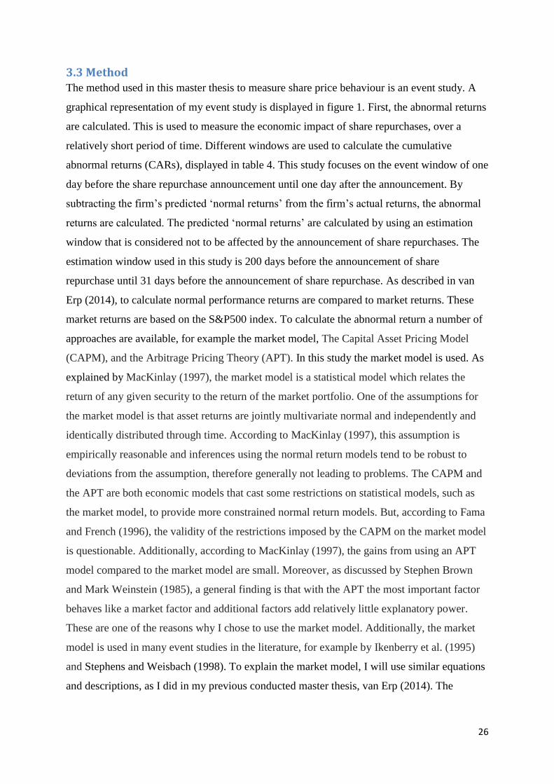
3.3 Method The method used in this master thesis to measure share price behaviour is an event study. A
graphical representation of my event study is displayed in figure 1. First, the abnormal returns
are calculated. This is used to measure the economic impact of share repurchases, over a
relatively short period of time. Different windows are used to calculate the cumulative
abnormal returns (CARs), displayed in table 4. This study focuses on the event window of one
day before the share repurchase announcement until one day after the announcement. By
subtracting the firm’s predicted ‘normal returns’ from the firm’s actual returns, the abnormal
returns are calculated. The predicted ‘normal returns’ are calculated by using an estimation
window that is considered not to be affected by the announcement of share repurchases. The
estimation window used in this study is 200 days before the announcement of share
repurchase until 31 days before the announcement of share repurchase. As described in van
Erp (2014), to calculate normal performance returns are compared to market returns. These
market returns are based on the S&P500 index. To calculate the abnormal return a number of
approaches are available, for example the market model, The Capital Asset Pricing Model
(CAPM), and the Arbitrage Pricing Theory (APT). In this study the market model is used. As
explained by MacKinlay (1997), the market model is a statistical model which relates the
return of any given security to the return of the market portfolio. One of the assumptions for
the market model is that asset returns are jointly multivariate normal and independently and
identically distributed through time. According to MacKinlay (1997), this assumption is
empirically reasonable and inferences using the normal return models tend to be robust to
deviations from the assumption, therefore generally not leading to problems. The CAPM and
the APT are both economic models that cast some restrictions on statistical models, such as
the market model, to provide more constrained normal return models. But, according to Fama
and French (1996), the validity of the restrictions imposed by the CAPM on the market model
is questionable. Additionally, according to MacKinlay (1997), the gains from using an APT
model compared to the market model are small. Moreover, as discussed by Stephen Brown
and Mark Weinstein (1985), a general finding is that with the APT the most important factor
behaves like a market factor and additional factors add relatively little explanatory power.
These are one of the reasons why I chose to use the market model. Additionally, the market
model is used in many event studies in the literature, for example by Ikenberry et al. (1995)
and Stephens and Weisbach (1998). To explain the market model, I will use similar equations
and descriptions, as I did in my previous conducted master thesis, van Erp (2014). The

27
equations plus descriptions for the abnormal return (AR) and the cumulative abnormal return
(CAR) are obtained from my study van Erp (2014).
Based on the market model the abnormal return is:
𝐴𝑅𝑖𝑡 = 𝑅𝑖𝑡- (𝛼𝑖 + 𝛽𝑖 𝑅𝑚𝑡),
hereby 𝐴𝑅𝑖𝑡 = abnormal return on stock i for day t; 𝑅𝑖𝑡 = return on stock i for day t; 𝛼𝑖 =
constant; 𝛽𝑖 =beta of stock i; and 𝑅𝑚𝑡 = return on the market portfolio for day t
The sum of the abnormal returns results in the cumulative abnormal return.
𝐶𝐴𝑅𝑖(𝑡1,𝑡2) = ∑ 𝐴𝑅𝑖𝑡𝑡2𝑡1 ,
where t1= the beginning day of the event window; t2= the last day of the event window; 𝐴𝑅𝑖𝑡
= abnormal return on stock i for day t. So 𝐶𝐴𝑅𝑖,(𝑡1,𝑡2) stands for the cumulative abnormal
return within the event window for each firm.
Finally to calculate the cumulative average abnormal return (CAAR), the average of all the
firm’s CARs is taken.
𝐶𝐴𝐴𝑅(𝑡1,𝑡2) =1
𝑁 ∑ 𝐶𝐴𝑅𝑖(𝑡1,𝑡2)
𝑡2𝑡1 ,
where t1= the beginning day of the event window; t2= the last day of the event window; N=
the total number of share repurchase announcements, which corresponds with the total
number of firms; and 𝐶𝐴𝑅𝑖 = cumulative abnormal return on stock i for day t. So 𝐶𝐴𝐴𝑅(𝑡1,𝑡2)
stands for the cumulative average abnormal return within the event window for the entire
sample.
By running an ordinary least squares (OLS) regression on the market model the estimates of
𝛼𝑖 and 𝛽𝑖 are obtained.

28
To test for possible explanations for the relation between share repurchase announcement and
share price behaviour, a time series OLS regressions is used. To test the five hypothesis
explained in chapter 2.2, several variables are used, explained in chapter 3.2. An important
assumption of OLS regressions is that the errors in the independent variable are negligible. In
order for the OLS estimators to be consistent, the independent variables in the OLS regression
are considered to be exogenous and there is no perfect multicollinearity. So, the explanatory
variables are contemporaneously exogenous of the error process. Furthermore, the variance of
the residuals is homogenous, and the errors are uncorrelated between observations. Also, the
OLS estimators are asymptotically normally distributed.
Exogeneity: E(ε𝑖 |𝑥𝑖) = 0 for all i = 1, …, n,
Where, ε𝑖 = the error term; and 𝑥𝑖 = the vector of explanatory variables.
And the variance of the error term is constant for each observation, resulting in:
Homoscedasticity: Var(ε𝑖 |𝑥𝑖) = 𝜎2
Figure 1
Event study
This figure displays the estimation window, event window, and the share repurchase announcement date. The estimation window is 200 before the announcement of share repurchase until 31 days before the announcement date. The event window is one day before until one day after the announcement of share repurchase. Finally, the share repurchase announcement is on day 0. The graphical representation is based on the design provided in van Erp (2014).
29
where, ε𝑖 = the error term; 𝑥𝑖 = the vector of explanatory variables; and 𝜎2 = variance of the
error term
Furthermore, the errors are uncorrelated between observations:
No autocorrelation: E(ε𝑖ε𝑗 |𝑥𝑖𝑇) = 0 for i ≠ j,
where, ε𝑖 and ε𝑗 are the error terms for different observations; and 𝑥𝑖𝑇 = the transposed vector
of explanatory variables.
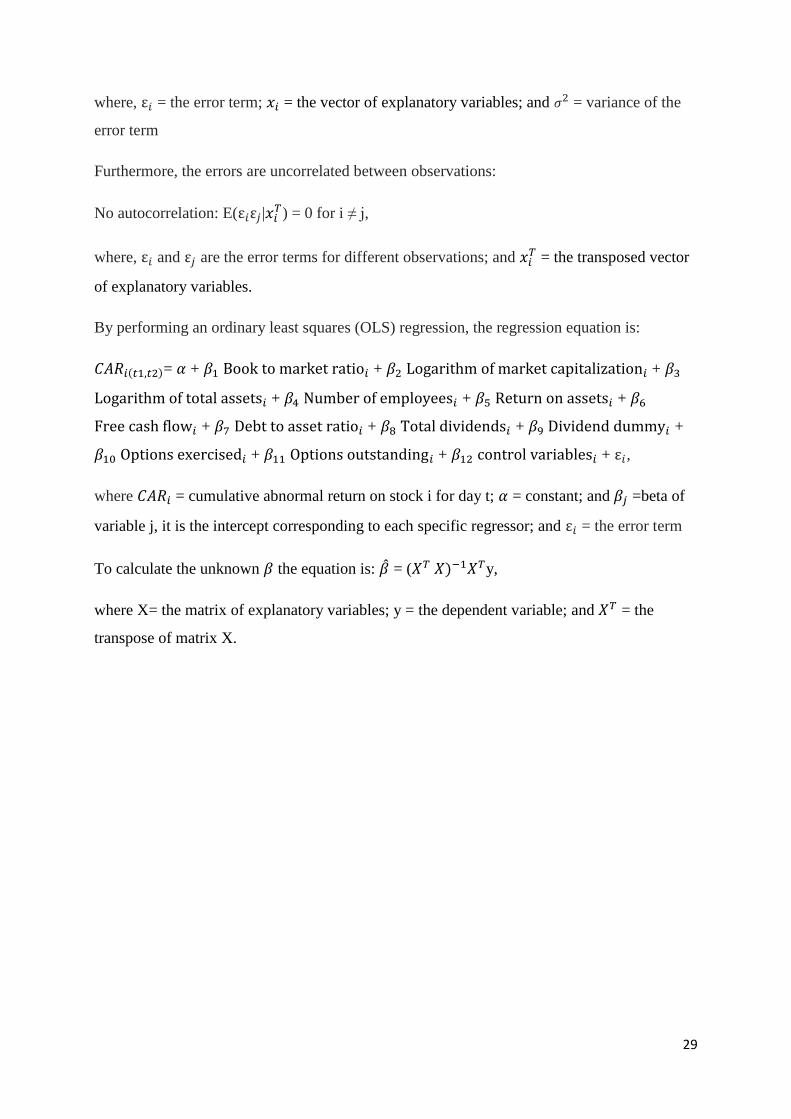
By performing an ordinary least squares (OLS) regression, the regression equation is:
𝐶𝐴𝑅𝑖(𝑡1,𝑡2)= 𝛼 + 𝛽1 Book to market ratio𝑖 + 𝛽2 Logarithm of market capitalization𝑖 + 𝛽3
Logarithm of total assets𝑖 + 𝛽4 Number of employees𝑖 + 𝛽5 Return on assets𝑖 + 𝛽6
Free cash flow𝑖 + 𝛽7 Debt to asset ratio𝑖 + 𝛽8 Total dividends𝑖 + 𝛽9 Dividend dummy𝑖 +
𝛽10 Options exercised𝑖 + 𝛽11 Options outstanding𝑖 + 𝛽12 control variables𝑖 + ε𝑖,
where 𝐶𝐴𝑅𝑖 = cumulative abnormal return on stock i for day t; 𝛼 = constant; and 𝛽𝑗 =beta of
variable j, it is the intercept corresponding to each specific regressor; and ε𝑖 = the error term
To calculate the unknown 𝛽 the equation is: �̂� = (𝑋𝑇 𝑋)−1𝑋𝑇y,
where X= the matrix of explanatory variables; y = the dependent variable; and 𝑋𝑇 = the
transpose of matrix X.

30
Chapter 4. Empirical analysis
4.1 Empirical results To find possible abnormal returns for the days around the announcement of share repurchase,
an event study is conducted. This event study is conducted for several windows around the
announcement day. Table 4 displays the cumulative average abnormal returns (CAARs) for
nine different windows. This is the average of all the cumulative abnormal returns (CARs) for
all the firms for each of the displayed windows. Moreover, in table A12 in the appendix this is
also displayed for the three different indexes, namely: NYSE, NASDAQ, and AMEX. Most
of the CAARs are positive, but not all of them are statistically significant. The CAAR for the
window [-1,1] is 0.04, this is statistically significant 4 at the 1% significance level. The
window [-1,1] is often used in the literature to test for short term abnormal performance. This
window will also mainly be used in this study. The positive CAAR provides evidence for the
hypothesis that share repurchases have a positive effect on firm performance. Besides, the
window [-10,-2] is used to test the relation between share repurchases and prior stock
performance. The selected window is based on past literature, such as Ikenberry et al. (1995).
The corresponding CAAR is -0.07 and it is statistically significant, at the 5% significance
level. This provides evidence for the mispricing hypothesis. As argued by Stephens and
Weisbach (1998), firms adjust their share repurchase behaviour based on the perceived
undervaluation. It supports the hypothesis that managers tend to repurchase shares when the
share price is in a period of decline.
There might be several explanations why share repurchase affects share price behaviour. This
is tested by investigating the relation between independent- and control variables, explained in
chapter 3.2, on the CARs of share repurchase. It is tested by using an ordinary least squares
(OLS) regression. These results are discussed in this section.
4 The default level for statistical significance throughout the rest of this study is set to a 10% statistical significance level. So, with statistical significance I mean the statistical significance at a 10% level. If the statistical significance level is different, this is mentioned explicitly.

31
Figure 2
Theoretical framework
This figure displays the theoretical framework including all the dependent and independent variables. The dependent variable is the cumulative abnormal return for share repurchase, based on the window 1 day before until one day after the announcement of share repurchase. In my analysis I test if the independent variable affects the dependent variable. The plus or minus sign stands for the predicted positive or negative relation the independent variable has with the dependent variable, based on the theory. The design of the framework is based on the theoretical framework provided in van Erp (2014)

32
To test for the mispricing hypothesis, the free cash flow hypothesis, the earnings per share
dilution hypothesis, the leverage hypothesis, and the tax benefits hypothesis, several
independent variables are used. For each of the independent variables I came up with a
hypothesis. The theoretical framework is displayed in figure 2. The design of the framework
is based on the theoretical framework provided in van Erp (2014). For each regression
coefficient, the tested null hypothesis is that the coefficient is equal to zero. The 𝐻1hypothesis
is that the coefficient is not equal to zero. The 𝐻0 hypothesis for each of the statements below
is:
The independent variable does not affect the firm’s CARs. The associated 𝐻1 hypotheses for
this are the following:
1. The book to market ratio affects the firm’s CARs.
2. The natural logarithm of total assets affects the firm’s CARs.
3. The natural logarithm of market capitalization affects the firm’s CARs.
4. The total number of employees affects the firm’s CARs.
5. The free cash flow affects the firm’s CARs.
6. The return on assets ratio affects the firm’s CARs.
7. The options outstanding affects the firm’s CARs.
8. The options exercised affects the firm’s CARs.
9. The debt to asset ratio affects the firm’s CARs.
10. The percentage of dividend affects the firm’s CARs.
11. The dividend dummy affects the firm’s CARs.
The results of this study are displayed in table 3.
Additionally, the sample is checked for multicollinearity, by analyzing the variance inflation
factor (VIF) scores. Furthermore, the correlations between the variables are analyzed. The
outcomes of the VIF analysis are displayed in table 7 and 8. To analyze possible
multicollinearity the magnitude of the VIF scores are analyzed. If the number is relatively
high it might signal multicollinearity. If this is the case the variable should be treated with
caution. In general, VIF scores higher than 10 are considered relatively high and might be up

33
for a closer examination. In my study the VIF scores of logarithm of market capitalization and
logarithm of total assets are greater than 10, displayed in table 7. Additionally, the variables
options outstanding and options exercised are close to 7 and considerably higher compared to
the rest. These variables are related, the higher VIF values indicate that one of these variables
is possibly redundant.
Moreover, to further analyze the relations between the variables, a correlation table is
analyzed, displayed in the tables 9a and 9b. The proxies for firm size all have relatively high
correlations among them, and measure the same thing. For example, the correlation between
logarithm of market capitalization and logarithm of total assets is 0.91, and between logarithm
of market capitalization and number of employees 0.38. Furthermore the correlation between
options outstanding and options exercised is 0.91. The correlation between percentage of
dividend and dividend dummy is 0.42. So, these variables show relatively high correlations.
To test differences between the variances of these variables, a variance-comparison test is
performed. In these tests the 𝐻0 hypothesis is: the difference between the variables’ variance
is equal to zero. The corresponding 𝐻1 hypothesis is: the difference between the variables’
variance is unequal to zero. For all of the tests, except for the test between the variance of the
logarithm of market capitalization and the variance of the logarithm of total assets, the 𝐻0
hypothesis can be rejected, at the 1% significance level. So, most of these variables’ variances
are considered different from each other. Furthermore, I performed a t-test to test the 𝐻0
hypothesis: the difference between the mean logarithm of market capitalization and the mean
logarithm of total assets is equal to zero. The corresponding 𝐻1 hypothesis is: the difference
between the mean logarithm of market capitalization and the mean logarithm of total assets is
unequal to zero. For this test, the 𝐻0 hypothesis can be rejected, at the 1% significance level.
In my regression tables with dependent variable CAR for share repurchase, all of the columns
4 consist of an OLS-regression with all the independent- and control variables together.
However, because of the possibility of multicollinearity, I included only one proxy variable
for size in each of the columns 1, 2, and 3, namely: logarithm of market capitalization,
logarithm of total assets, and number of employees, respectively. Furthermore, I also included
only one variable related to options in the columns 1 to 3. So, either options outstanding or
options exercised. Finally, I only included one variable related to dividends in the columns 1
to 3. So, either dividend dummy or percentage of dividend. The VIF scores for these
regressions are displayed in table 8. All of these VIF scores are much lower than 10.
34
Furthermore, to test for heteroskedasticity of residuals, the White’s test and the Breusch-
Pagan test are conducted, displayed in table A18 and A19. Hereby, the 𝐻0 hypothesis is: the
variance of residuals is homogenous. The corresponding 𝐻1 hypothesis is: the variance of
residuals is not homogenous. These results are based on the regression displayed in table 5
column 4. For both tests, the 𝐻0 hypothesis cannot be rejected.
4.1.1 The effect of the book to market ratio on the firm’s CARs
For the book to market ratio I predicted it to have a positive effect on the firm’s CARs,
because firms with a high book to market ratio are considered to have value stocks, and firms
with a low book to market ratio are considered to have growth stocks. If the book to market
ratio is larger than 1, the share is considered to be undervalued. And, as concluded by
Ikenberry, Lakonishok and Vermaelen (1995), value stocks are more likely to have
undervaluation as their primary motivation. So, the announcement of repurchasing stock
would have a greater positive impact on the CARs compared to growth stocks. As predicted, I
find a positive relation between the book to market ratio and the firm’s CARs, displayed in
table 5. Moreover, the value in column 2 is 0.040. This is statistically significant different
from zero, at my default significance level of 10%5. As displayed in column 3, when the
number of employees is used as a proxy for size, instead of market capitalization and the
logarithm of total assets, the value is 0.049 and statistically significant, at the significance
level of 5%. Therefore, the 𝐻0 hypothesis: book to market ratio does not affect the firm’s
CARs, can be rejected, at the 5% significance level. So these results provide evidence for the
mispricing hypothesis.
4.1.2 The effect of the logarithm of total assets on the firm’s CARs
The natural logarithm of total assets is a proxy for firm size. For the natural logarithm of total
assets I predicted it to have a negative effect on the firm’s CARs, because smaller firms are
considered to have higher levels of information asymmetry. The higher levels of information
asymmetry lead to higher abnormal returns because managers are most likely to be better
informed about the financial and operational conditions of the firm. As predicted, I find a
negative relation between the natural logarithm of total assets and the firm’s CARs, displayed
in table 5 column 2. The value in column 2 is -0.020, it is statistically significant, at the 1%
significance level. Therefore, the 𝐻0 hypothesis: natural logarithm of total assets does not
5 The default level for statistical significance throughout the rest of this study is set to a 10% statistical significance level. So, with statistical significance I mean the statistical significance at a 10% level. If the statistical significance level is different, this is mentioned explicitly.

35
affect the firm’s CARs, can be rejected, at the 1% significance level. These results show
support for the mispricing hypothesis.
4.1.3 The effect of the natural logarithm of market capitalization on the firm’s CARs
Furthermore, the logarithm of market capitalization is another proxy for firm size. I predicted
it to have a negative effect on the firm’s CARs. Again, this is based on the difference in
information asymmetry. So, smaller firms are considered to have higher levels of information
asymmetry. The higher levels of information asymmetry could lead to higher abnormal
returns because managers are most likely to be better informed about the financial and
operational conditions of the firm. As predicted, I find a negative relation between the natural
logarithm of market capitalization and the firm’s CARs, displayed in table 5 columns 1 and 4.
Only the value of -0,021 in column 1 is statistically significant, at the 1% significance level.
So, based on this result, the 𝐻0 hypothesis: market capitalization does not affect the firm’s
CARs, can be rejected, at the 1% significance level. Moreover, it provides evidence to support
the mispricing hypothesis.
4.1.4 The effect of the total number of employees on the firm’s CARs
Also, the number of employees is used as a proxy of firm size. I predicted it to have a
negative effect on the firm’s CARs. Because this is also proxy of firm size, the prediction is
the same as for the logarithm of total assets and market capitalization. So, smaller firms are
considered to have higher levels of information asymmetry. The higher levels of information
asymmetry could lead to higher abnormal returns because managers are most likely to be
better informed about the financial and operational conditions of the firm. As predicted, I find
a negative relation between the total number of employees and the firm’s CARs, displayed in
table 5 columns 3 and 4. However, these variables are not statistically significant.
Furthermore, the economic significance is low, because both values are smaller than 0.001.
So, the 𝐻0 hypothesis: the number of employees does not affect the firm’s CARs, cannot be
rejected. Moreover, it does not provide evidence to support the mispricing hypothesis.
4.1.5 The effect of the free cash flow on the firm’s CARs
For the free cash flow I predicted it to have a positive effect on the firm’s CARs, because a
high amount of free cash flow could be the cause of agency problems. So, firms with high
levels of free cash flow could benefit the most from repurchasing shares. Because, otherwise
managers could use the excess cash flow to invest in negative net present value projects, or
managers could engage in empire building or fringe benefit consumption. Additionally,
Managers could hold on to underperforming subordinates for too long, because of the excess

36
of cash flow. Repurchasing shares reduces the excess free cash flow, and therefore reducing
the managers’ power. As argued by Jensen (1986), managers are more constrained after
reducing the excess free cash flow. In contrast of what I predicted, I find mixed results. As
displayed in table 5, the values for free cash flow are positive in column 1 and 3, and negative
in column 2 and 4. But none of these values are statistically significant. Additionally, the
economic impact is considered low, since all the values are 0.001 or smaller. So, the 𝐻0
hypothesis: free cash flow does not affect the firm’s CARs, cannot be rejected. Moreover, it
does not provide enough evidence to support the free cash flow hypothesis.
4.1.6 The effect of the return on assets ratio on the firm’s CARs
For the return on assets I predicted it to have a positive effect on the firm’s CARs, because a
higher return on assets could be a reason for higher agency costs, because the return on assets
is related to free cash flow. So, firms with a high level of return on asset could benefit the
most from repurchasing shares. As argued before, managers could use the excess cash flow to
invest in negative net present value projects, or managers could engage in empire building or
fringe benefit consumption. Managers could also hold on to underperforming subordinates for
too long, because of the excess of cash flow. In contrast of what I predicted, I find mixed
results among the different regressions I used. For example, in table 5 the value for the return
on assets is negative in column 2 and 3, but positive in column 1 and 4. Namely, the exact
values are: 0.004, -0.006, -0.021 and 0.010 respectively. Additionally in table 6 all the values
for the returns on assets in all the columns are positive. A possible explanation for the positive
relation between the return on assets and the firm’s CARs is that having higher levels of
return on assets could signal financial strength when financially healthy firms repurchase
shares. Furthermore, firms with high levels of return on assets benefit the most from share
repurchases because of the possible reduction in agency cost. However, for all of the values
mentioned in the tables 5 and 6 the results are not statistically significant. So, the 𝐻0
hypothesis: return on assets does not affect the firm’s CARs, cannot be rejected. Moreover, it
does not provide enough evidence to support the free cash flow hypothesis.
4.1.7 The effect of the options outstanding on the firm’s CARs
For the options exercised I predicted it to have a negative effect on the firm’s CARs, because
earnings per share dilution is negatively valued by managers. For example, Bens et al. (2003)
find an increase in the level of stock repurchases when the dilutive effect of outstanding
employee stock options on diluted EPS increases. Additionally, Brav et al. (2005) find that
two-thirds of their survey respondents feel that offsetting dilution is an important or very

37
important factor affecting their repurchase decisions. In contrast of the predicted negative
effect, I find a positive relation between the options exercised and the firm’s CARs. Displayed
in table 5, the value for options exercised is positive in all columns. I do not know the reason
why this relation might be positive. However the values are not statistically significant.
Moreover, the impact is considered to be small, because the values are 0.001 or smaller. So,
the 𝐻0 hypothesis: options exercised does not affect the firm’s CARs, cannot be rejected.
Moreover, it does not provide evidence to support the earnings per share dilution hypothesis.
4.1.8 The effect of the options exercised on the firm’s CARs
For the options outstanding I predicted it to have a negative effect on the firm’s CARs,
because earnings per share dilution is negatively valued by managers. This follows the same
reasoning as explained above for the options exercised variable. In contrast of what I
predicted, I find a positive relation between the options outstanding and the firm’s CARs. As
displayed in table 6, the values for options outstanding are positive in all the columns. Again,
I do not know the reason why this relation might be positive. But, also these values are not
statistically significant. Moreover, the economic impact is considered to be small, because the
values are all smaller than 0.001. So, the 𝐻0 hypothesis: options outstanding does not affect
the firm’s CARs, cannot be rejected. Moreover, it does not provide evidence to support the
earnings per share dilution hypothesis.
4.1.9 The effect of the debt to asset ratio on the firm’s CARs
For the debt to asset ratio I predicted it to have a positive effect on the firm’s CARs, because
an increase in the debt to asset ratio could lead to a more beneficial leverage ratio. This could
be beneficial for firms, because of the effects of tax benefits of interest payments associated
with adjusting the firm’s capital structure. Modigliani and Miller (1958, 1963) opened the
discussion in scientific research about adjusting the capital structure in order to find a more
optimal leverage ratio. In line with the prediction, I find a positive relation between the debt
to asset ratio and the firm’s CARs. Displayed in table 5, the values for the debt to asset ratio
for all the columns are positive. For example the value in column 1 is 0.077. However these
results are not statistically significant. So, despite the positive relation, the 𝐻0 hypothesis:
debt to asset ratio does not affect the firm’s CARs, cannot be rejected. Moreover, it does not
provide enough evidence to support the leverage hypothesis.
4.1.10 The effect of the percentage of dividend on the firm’s CARs
For the dividend dummy I predicted it to have a negative effect on the firm’s CARs, because
share repurchases could be more beneficial to shareholders than dividends. Share repurchases

38
might be more beneficial for shareholders, because of tax benefits. As stated by Black (1976),
a corporation that pays no dividends will be more attractive to taxable individual investors
than a similar corporation that pays dividends, when dividends are taxed more heavily than
capital gains, and where capital gains are not taxed until realized. In line with the prediction, I
also find a negative relation between the dividend dummy and the firm’s CARs. Displayed in
table 6, the value for dividend dummy is negative for all of the columns. Moreover, the value
-0.042 in column 3 is statistically significant. Also, in column 4 the value is statistically
significant. So these results are statistically significant different from zero. Therefore, the 𝐻0
hypothesis: dividend dummy does not affect the firm’s CARs, can be rejected, at the 10%
significance level. These results provide evidence for the tax benefits hypothesis.
4.1.11 The effect of the dividend dummy on the firm’s CARs
For the percentage of dividend I predicted it to have a negative effect on the firm’s CARs,
because share repurchases could be more beneficial to shareholders than dividends. So having
a higher ratio of dividends negatively influences the firm’s abnormal return. This is because
share repurchase might be more beneficial for shareholders, because of tax benefits. In
contrast of what I predicted, I find a positive relation between the percentage of dividend and
the firm’s CARs. Displayed in table 5, the value for percentage of dividend is positive in all
the columns. The value 0.8222 is statistically significant. However, in the columns 1, 2, and 3
the value isn’t statistically significant. Also, as I explain in chapter 4.2, column 4 is
considered to have less explanatory power, because there might be some level of
multicollinearity. Therefore, the 𝐻0 hypothesis: percentage of dividend does not affect the
firm’s CARs, cannot be completely rejected. Additionally the predicted negative relation
between the percentage of dividend and the firm’s CARs is not found. So, it does not provide
evidence to support the tax benefits hypothesis.
Finally, the industry dummies also seem to affect the firm’s CARs. Displayed in table 5, the
values for the manufacturing industry dummy and the service industry dummy are all negative
in all the columns. By executing the regression in STATA the dummy variable for the group
of remaining industries is automatically omitted. Hereby, the manufacturing industry dummy
and the service industry dummy are compared on the dummy variable for the group of
remaining industries. The value for service industry dummy in column 1, 2, and 3 is
negatively statistically significant. This is also the case in all the other regression tables. For
example, the value in table 5 column 1 is -0.064. This suggests that firms from the service
industry experience lower abnormal returns from share repurchases, compared to other

39
industries. The reason for this might be up for further investigation. On the other hand, the
values for the manufacturing industry dummy are not statistically significant.
Table 4
Overview of the Cumulative average abnormal returns (CAARs)
This table displays the CAARs of the full sample for different windows. The windows are measured in days around the announcement day of share repurchases; hereby the share repurchase announcement day is 0. Furthermore it displays the standard error, t-statistic, and the probability.
Table 3
Overview prediction and results for all the hypotheses
This table displays the prediction and results for all the hypotheses. To test for the mispricing hypothesis, four independent variables are used. To test for the free cash flow hypothesis two variables are used. To test for the earnings per share dilution hypothesis 2 variables are used. To test for the leverage hypothesis one variable is used. Finally, to test for the tax benefits hypothesis two variables are used. The column ‘Prediction’ displays whether the relation on the cumulative abnormal return (CAR), with a window of 1 day before until 1 day after the share repurchase announcement, is expected to be positive or negative. After conducting multiple OLS-regressions, the conclusive results are displayed in the last three columns.
window CAAR Std. Error t-stat. prob.
[-1,1] 0.04 0.01 3.90 0.00
[-3,3] 0.03 0.02 1.35 0.18
[-5,1] -0.29 0.32 -0.91 0.37
[-5,5] 0.01 0.03 0.42 0.68
[-10,-2] -0.07 0.03 -2.31 0.02
[-10,10] -0.03 0.06 -0.52 0.60
[-15,1] 0.10 0.12 0.80 0.43
[-15,15] 0.10 0.14 0.71 0.48
[-30,30] -0.13 0.19 -0.69 0.49
Hypothesis Variable Prediction Result Statistical significance of result Supports hypothesis
Mispricing hypothesis Book to market ratio + + Significant** Yes
Logarithm of total assets - - Significant*** Yes
Logarithm of market capitalization - - Significant*** Yes
Number of employees - - Not significant No
Free cash flow hypothesis Free cash flow + +/- Not significant No
Return on Assets + +/- Not significant No
Earnings per share dilution hypothesis Options exercised - + Not significant No
Options outstanding - + Not significant No
Leverage hypothesis Debt to asset ratio + + Not significant No
Tax benefits hypothesis Dividend dummy - - Significant* Yes
Percentage of dividend - + Significant* No
*** p<0.01, ** p<0.05, * p<0.1

40
Table 5
Regression results with dependent variable Cumulative abnormal return (CAR)
This table displays the regression results for every selected independent variable. The dependent variable is CAR for share repurchase. This is based on the window, one day before until one day after the announcement of share repurchase. The results are obtained by using an ordinary least squares (OLS) regression. The first displayed value of every independent variable is the regression coefficient, the value between parentheses is the standard error. Column 4 reports the regression results where all independent- and control variables are included. In columns 1, 2, and 3, only one measure of firm size is included in the regression. These are logarithm of market capitalization, logarithm of total assets, and the number of employees respectively. Additionally, in column 1, 2, and 3, to test for the earnings per share dilution hypothesis, only options exercised is used. In column 4, options outstanding is added to the test. Furthermore, to test for the tax benefits hypothesis, only the percentage of dividend is used in column 1, 2, and 3. In column 4, dividend dummy is also added to the test.
(1) (2) (3) (4)
VARIABLES CAR CAR CAR CAR
Book to market ratio 0.018 0.040* 0.049** 0.022
(0.026) (0.024) (0.024) (0.037)
Logarithm of total assets -0.020*** 0.001
(0.008) (0.027)
Logarithm of market capitalization -0.021*** -0.017
(0.008) (0.027)
Number of employees -0.000 -0.000
(0.000) (0.000)
Free cash flow 0.000 -0.000 0.001 -0.000
(0.007) (0.007) (0.007) (0.007)
Return on Assets 0.004 -0.006 -0.021 0.010
(0.087) (0.087) (0.087) (0.088)
Options exercised 0.001 0.001 0.000 0.001
(0.001) (0.001) (0.001) (0.003)
Options outstanding 0.000
(0.001)
Debt to asset ratio 0.077 0.115 0.044 0.091
(0.075) (0.079) (0.074) (0.091)
Dividend dummy -0.052*
(0.028)
Percentage of dividend 0.466 0.447 0.469 0.822*
(0.399) (0.399) (0.401) (0.447)
Percentage of capital expenditures -0.058 -0.064 -0.063 -0.054
(0.226) (0.226) (0.227) (0.226)
Manufacturing industry dummy -0.035 -0.037 -0.034 -0.037
(0.032) (0.032) (0.033) (0.033)
Service industry dummy -0.064* -0.064* -0.048 -0.070*
(0.037) (0.037) (0.036) (0.037)
Constant 0.179** 0.157** 0.026 0.163**
(0.071) (0.065) (0.040) (0.075)
Observations 749 749 749 749
R-squared 0.020 0.020 0.012 0.025
Standard errors in parentheses
*** p<0.01, ** p<0.05, * p<0.1

41
(1) (2) (3) (4)
VARIABLES CAR CAR CAR CAR
Book to market ratio 0.019 0.039 0.046* 0.022
(0.026) (0.024) (0.024) (0.037)
Logarithm of total assets -0.018** 0.001
(0.008) (0.027)
Logarithm of market capitalization -0.018** -0.017
(0.008) (0.027)
Number of employees -0.000 -0.000
(0.000) (0.000)
Free cash flow 0.000 -0.000 0.000 -0.000
(0.007) (0.007) (0.007) (0.007)
Return on Assets 0.033 0.023 0.015 0.010
(0.087) (0.086) (0.086) (0.088)
Options exercised 0.001
(0.003)
Options outstanding 0.000 0.000 0.000 0.000
(0.000) (0.000) (0.000) (0.001)
Debt to asset ratio 0.085 0.118 0.060 0.091
(0.075) (0.079) (0.074) (0.091)
Dividend dummy -0.030 -0.028 -0.042* -0.052*
(0.025) (0.025) (0.024) (0.028)
Percentage of dividend 0.822*
(0.447)
Percentage of capital expenditures -0.060 -0.065 -0.064 -0.054
(0.226) (0.226) (0.226) (0.226)
Manufacturing industry dummy -0.035 -0.036 -0.032 -0.037
(0.032) (0.032) (0.033) (0.033)
Service industry dummy -0.066* -0.066* -0.053 -0.070*
(0.037) (0.037) (0.036) (0.037)
Constant 0.176** 0.155** 0.045 0.163**
(0.072) (0.065) (0.041) (0.075)
Observations 749 749 749 749
R-squared 0.021 0.020 0.015 0.025
Standard errors in parentheses
*** p<0.01, ** p<0.05, * p<0.1
Table 6
Regression results with dependent variable Cumulative abnormal return (CAR)
This table displays the regression results for every selected independent variable. The dependent variable is CAR for share repurchase. This is based on the window, one day before until one day after the announcement of share repurchase. The results are obtained by using an ordinary least squares (OLS) regression. The first displayed value of every independent variable is the regression coefficient, the value between parentheses is the standard error. Column 4 reports the regression results where all independent- and control variables are included. In columns 1, 2, and 3, only one measure of firm size is included in the regression. These are logarithm of market capitalization, logarithm of total assets, and the number of employees respectively. Additionally, in column 1, 2, and 3, to test for the earnings per share dilution hypothesis, only options outstanding is used. In column 4, options exercised is added to the test. Furthermore, to test for the tax benefits hypothesis, only the dividend dummy is used in column 1, 2, and 3. In column 4, the percentage of dividend is also added to the test.

42
Table 7
The variance inflation factor (VIF) scores for all the independent- and control variables
This table displays the VIF scores. All the independent- and control variables are included in this table. It
is a test for multicollinearity in an ordinary least squares regression analysis. Generally speaking a
variable whose VIF values are greater than 10 may need to be investigated further.
Variable VIF 1/VIF
Logarithm of market capitalization 19.20 0.052092
Logaritm of total assets 17.23 0.058043
Options outstanding 6.31 0.158518
Options exercised 6.17 0.161998
Book to market ratio 2.87 0.348960
Manufacturing industry dummy 2.05 0.488148
Service industry dummy 2.05 0.488973
Debt to asset ratio 1.65 0.605481
Dividend dummy 1.51 0.663286
Percentage of dividend 1.31 0.765767
Return on Assets 1.23 0.811819
Number of employees 1.23 0.815324
Percentage of capital expenditures 1.13 0.888316
Free cash flow 1.04 0.960984
Mean VIF 4.64
Table 8
The variance inflation factor (VIF) scores
This table displays the VIF scores. Several independent- and control variables are included in this table.
Only one variable for size is used, which is logarithm of market capitalization. Also, only one variable for
dividend is used. Furthermore, only one variable for options is used. The VIF scores test for
multicollinearity in an ordinary least squares regression analysis. Generally speaking a variable whose
VIF values are greater than 10 may need to be investigated further. These VIF scores are based on the
regression in table 5 column 1, but these scores are also representative for column 2 and 3. Moreover,
these scores are also representative for all the other regressions in the columns 1, 2, and 3 in all the
regression tables, because the scores are very similar and all below 10.
Variable VIF 1/VIF
Service industry dummy 2.02 0.494280
Manufacturing industry dummy 2.01 0.498436
Logarithm of market capitalization 1.61 0.620937
Book to market ratio 1.44 0.696703
Return on Assets 1.21 0.829004
Options exercised 1.18 0.850846
Percentage of capital expenditures 1.12 0.889497
Debt to asset ratio 1.10 0.907766
Percentage of dividend 1.04 0.960761
Free cash flow 1.03 0.966324
Mean VIF 1.38

43
Tab
le 9
a
The
corr
elat
ion
tab
le
This
tab
le d
isp
lays
th
e co
rrel
atio
ns
bet
we
en a
ll th
e in
dep
end
ent-
an
d c
on
tro
l var
iab
les.
Th
e to
tal t
able
is
split
up
into
tw
o p
iece
s to
mak
e it
fit
on
th
e p
age.
Tab
le 9
b c
on
tain
s th
e o
ther
hal
f o
f th
e ta
ble
.
Book
to m
arke
t rat
ioLo
garit
m o
f tot
al a
sset
sLo
g M
arke
t cap
italiz
atio
n N
umbe
r of e
mpl
oyee
sFr
ee ca
sh fl
ow%
of c
apita
l exp
endi
ture
sRe
turn
on
Asse
tsO
ptio
ns e
xerc
ised
Book
to m
arke
t rat
io1.
00
Loga
ritm
of t
otal
ass
ets
-0.1
849
1.00
Loga
ritm
of M
arke
t cap
italiz
atio
n -0
.470
10.
9098
1.00
Num
ber o
f em
ploy
ees
-0.0
403
0.37
520.
3309
1.00
Free
cash
flow
-0.0
976
-0.0
006
0.02
27-0
.023
81.
00
% o
f cap
ital e
xpen
ditu
res
-0.0
480
0.06
580.
0510
0.03
27-0
.009
01.
00
Retu
rn o
n As
sets
-0.3
232
0.10
920.
2502
0.03
31-0
.024
2-0
.012
51.
00
Opt
ions
exe
rcis
ed
-0.1
036
0.30
410.
3435
0.20
550.
0409
-0.0
435
0.05
471.
00
Opt
ions
out
stan
ding
-0.0
975
0.32
920.
3623
0.23
060.
0272
-0.0
462
0.03
880.
9138
Debt
to a
sset
ratio
-0.0
622
0.33
700.
1674
0.06
170.
1251
0.16
23-0
.100
7-0
.011
5
Divi
dend
dum
my
-0.1
008
0.37
110.
3391
0.22
30-0
.016
50.
0299
0.15
550.
0715
% o
f div
iden
d-0
.096
30.
0167
0.06
950.
0415
-0.0
023
-0.0
227
0.18
920.
0188
Man
ufac
turin
g in
dust
ry d
umm
y 0.
0017
0.04
600.
0608
-0.0
876
-0.0
374
-0.2
184
0.03
82-0
.038
4
Serv
ice
indu
stry
dum
my
-0.0
461
-0.1
688
-0.1
487
-0.0
059
0.07
510.
0068
-0.0
971
0.06
71
Rem
aini
ng in
dust
ry d
umm
y0.
0507
0.13
420.
0920
0.12
00-0
.037
90.
2746
0.06
20-0
.027
3

44
Tab
le 9
b
The
corr
elat
ion
tab
le
This
tab
le d
isp
lays
th
e co
rrel
atio
ns
bet
we
en a
ll th
e in
dep
end
ent-
an
d c
on
tro
l var
iab
les.
Th
e to
tal t
able
is
split
up
into
tw
o p
iece
s to
mak
e it
fit
on
th
e p
age.
Tab
le 9
a co
nta
ins
the
oth
er h
alf
of
the
tab
le.
Opt
ions
out
stan
ding
Debt
to a
sset
ratio
Divi
dend
dum
my
% o
f div
iden
dM
anuf
actu
ring
indu
stry
dum
my
Serv
ice
indu
stry
dum
my
Rem
aini
ng in
dust
ry d
umm
y
Book
to m
arke
t rat
io
Loga
ritm
of t
otal
ass
ets
Loga
ritm
of M
arke
t cap
italiz
atio
n
Num
ber o
f em
ploy
ees
Free
cash
flow
% o
f cap
ital e
xpen
ditu
res
Retu
rn o
n As
sets
Opt
ions
exe
rcis
ed
Opt
ions
out
stan
ding
1.00
Debt
to a
sset
ratio
-0.0
076
1.00
Divi
dend
dum
my
0.07
850.
1353
1.00
% o
f div
iden
d0.
0364
-0.0
295
0.42
201.
00
Man
ufac
turin
g in
dust
ry d
umm
y -0
.002
7-0
.044
20.
0880
0.03
061.
00
Serv
ice
indu
stry
dum
my
0.04
420.
0041
-0.1
580
-0.0
078
-0.6
700
1.00
Rem
aini
ng in
dust
ry d
umm
y-0
.047
20.
0524
0.06
75-0
.030
7-0
.524
1-0
.281
11.
00

45
4.2 Sensitivity analysis I tested for differences of the cumulative average abnormal returns (CAARs) between
different indexes. These indexes are: the NYSE, NASDAQ, and AMEX index. The CAARs
are displayed in table A12. Based on table 4, I concluded that the CAAR including all indexes
for the window one day before until one day after the announcement of share repurchase [-
1,1] is 0.04, this is statistically significant at the 1% significance level. Moreover, the values
for the CAARs for the window [-1,1] for all the different industries separately are all positive.
However, only the CAAR for the firms in the NASDAQ index is statistically significant, at
the 1% significance level. Moreover, to test for differences across the indexes I performed
three t-tests. In these tests I test if the differences between the mean CARs for the sample
including all indexes and the mean CARs for one particular index are equal to zero. Hereby,
the 𝐻0 hypothesis is: the difference between the mean CARs for the sample including all
indexes and the mean CAR for the particular index is equal to zero. The corresponding
alternative hypothesis 𝐻𝑎 is: the difference between the mean CAR for the sample including
all indexes and the mean CAR for the particular index is unequal to zero. Based on the p-
values of the two sided test, only the 𝐻0 hypothesis: the difference between the mean CAR for
the sample including all indexes and the mean CAR for the NYSE index is equal to zero, can
be rejected, at the 10% significance level. For the other two indexes, the 𝐻0 hypothesis is: the
difference between the mean CAR for the sample including all indexes and the mean CAR for
the particular index is equal to zero, cannot be rejected. Finally, also a control variable ‘Sales’
is added to the regressions. However, compared to table 5 the results are very similar, and it
doesn’t change anything about the final conclusions.

46
Chapter 5. Conclusion and discussion
In this study I provide evidence that share repurchase announcement positively affect share
price behaviour, because I found higher abnormal returns after share repurchase
announcements. This result is based on a window of 1 day before until 1 day after the
announcement of share repurchase, and statistically significant at the 1% significance level. In
table 4 this result is displayed.
Furthermore, I investigated five hypotheses, based on past literature. These hypotheses are:
the mispricing hypothesis, the free cash flow hypothesis, the earnings per share dilution
hypothesis, the leverage hypothesis, and the tax benefits hypothesis. The results are displayed
in table 3. First of all, I provide evidence for the mispricing hypothesis, because displayed in
table 4, the cumulative average abnormal return (CAAR) for the window [-10,-2] is -0.07, at
the 1% significance level. The window is 10 days before until 2 days before the
announcement of share repurchase. It supports the hypothesis that managers tend to
repurchase shares when the share price is in a period of decline. This provides support for
Stephens and Weisbach (1998), who state that firms adjust their share repurchase behaviour
based on the perceived undervaluation.
Moreover, I provide evidence for the mispricing hypothesis based on the book to market ratio.
I predicted it to have a positive effect on the firm’s CARs, because firms with a high book to
market ratio are considered to have value stocks, and firms with a low book to market ratio
are considered to have growth stocks. And if the book to market ratio is larger than 1, the
share is considered to be undervalued. As predicted, I found a positive relation between the
book to market ratio and the firm’s CARs, displayed in table 5. Moreover, the value in
column 2 is 0.040, at my default significance level of 10%6. This provides evidence that
supports the mispricing hypothesis.
Also, I provide evidence for the mispricing hypothesis based on the natural logarithm of total
assets as a proxy for firm size. I predicted it to have a negative effect on the firm’s CARs,
because smaller firms are considered to have higher levels of information asymmetry. As
predicted, I found a negative relation between the natural logarithm of total assets and the
6 The default level for statistical significance throughout the rest of this study is set to a 10% statistical significance level. So, with statistical significance I mean the statistical significance at a 10% level. If the statistical significance level is different, this is mentioned explicitly.

47
firm’s CARs, displayed in table 5 column 2. This relation is statistically significantly
negative, at the 1% significance level. The value for the natural logarithm of total assets in
table 5 column 2 is -0,020. The results show support for the mispricing hypothesis.
Next, I provide evidence for the mispricing hypothesis based on the natural logarithm of
market capitalization. I predicted it to have a negative effect on the firm’s CARs, because
smaller firms are considered to have higher levels of information asymmetry. As predicted, I
found a statistically significant negative relation between the natural logarithm of market
capitalization and the firm’s CARs, at the 1% significance level, displayed in table 5 column
1. The value for the natural logarithm of market capitalization in table 5 column 1 is -0,021.
These results show support for the mispricing hypothesis.
Additionally, I also tested the effect of the number of employees on the firm’s CARs. I
predicted it to have a negative relation, because smaller firms are considered to have higher
levels of information asymmetry. The values for the number of employees are negative as
predicted, displayed in table 5 column 3 and 4. However, these results are not statistically
significant. So, these results do not provide enough evidence to support the mispricing
hypothesis.
Next, I do not find enough evidence to support the free cash flow hypothesis based on the free
cash flow. I predicted the free cash flow to have a positive effect on the firm’s CARs, because
high amount of free cash flow could be the cause of agency problems. So, firms with high
levels of free cash flow could benefit the most from repurchasing shares, because of the
possible reduction in agency costs. I found mixed results for the relation between the free cash
flow and the firm’s CARs. As displayed in table 5, the value free cash flow is positive in
column 1 and 3, and negative in column 2 and 4. But none of these values are statistically
significant. So, it does not provide enough evidence to support the free cash flow hypothesis.
Also, based on the return on assets, the results do not provide evidence to support the free
cash flow hypothesis. For the return on assets I predicted it to have a positive effect on the
firm’s CARs, because firms with a high level of return on asset could benefit the most from
repurchasing shares, because of the possible reduction in agency cost. In contrast of what I
predicted, I found mixed results among the different regressions I used. For example, in table
5 the value for the return on assets is negative in column 2 and 3, but positive in column 1 and
4. But, none of these are statistically significant. So, it does not provide enough evidence to
support the free cash flow hypothesis.

48
Additionally, the results do not provide evidence to support the earnings per share dilution
hypothesis. For both the options outstanding and options exercised I predicted it to have a
negative effect on the firm’s CARs. However, in contrast of the predicted negative effect, I
found a positive relation with the firm’s CARs, displayed in table 5 and 6. But none of these
values are statistically significant. So it does not provide evidence to support the earnings per
share dilution hypothesis.
Based on the debt to asset ratio, the results do not provide enough evidence to support the
leverage hypothesis. For the debt to asset ratio I predicted it to have a positive effect on the
firm’s CARs. The reason for this is the tax benefits of interest payments associated with
adjusting one’s capital structure. As predicted, I found a positive relation between the debt to
asset ratio and the firm’s CARs. However, the results displayed in table 5 are not statistically
significant. So, it does not provide enough evidence to support the leverage hypothesis.
Finally, when testing for the tax benefits hypothesis, I found evidence to support the
hypothesis. This hypothesis is tested by the two variables, dividend dummy and percentage of
dividend. For both the variables I predicted it to have a negative effect on the firm’s CARs,
because share repurchases could be more beneficial to shareholders than dividends. This is
because of tax benefits. As predicted, I found a negative relation between the dividend
dummy and the firm’s CARs, displayed in table 6. In column 3 and 4, I found a statistically
significant negative value for dividend dummy. Namely, in column 3 the statistical significant
value is -0.042. These results support the tax benefits hypothesis. On the other hand, for the
percentage of dividend a positive relation on the firm’s CARs is found. In table 5 column 4
the value 0.8222 is statistically significant. So this might provide evidence against the tax
benefits hypothesis. But, as already explained in chapter 4.1, column 4 is considered to have
less explanatory power, because there might be some level of multicollinearity. To be more
specific, both the variables dividend dummy and percentage of dividend are very much
related. So the values in column 4 have to be treated with caution.
To conclude, I provide evidence to support the mispricing hypothesis and the tax benefit
hypothesis. On the other hand, I do not provide enough evidence to support the free cash flow
hypothesis, earnings per share dilution hypothesis, and the leverage hypothesis.
This study contributes to the Finance literature, because I explain the effects that multiple
variables could have on the firm’s CARs. The corresponding hypotheses about the effects of
multiple variables on the firm’s CARs are based on past literature. Furthermore, this study is

49
conducted over a relatively recent period of 2000 until 2012. Additionally, evidence is found
to support the mispricing hypothesis and the tax benefit hypothesis. I also provide evidence
for different abnormal returns because of share repurchases among different industries. This
might be interesting to investigate as part of future research. Besides, it would be interesting
to also test for the long term effect of share repurchase. Furthermore, the agency costs theory
could be investigated more specifically. I found evidence for the mispricing hypothesis, which
is related with agency costs. But it is for example interesting how this would relate to
manager’s compensation and ownership.
A limitation of this study is that the derived conclusions might not be generalizable for firms
in other countries, because the sample only includes firms listed on the NYSE, NASDAQ, and
AMEX. So, the effects might be different for other countries, for example due to regulation or
cultural differences. Another limitation of the study is that COMPUSTAT has some missing
data among firms. So, finally a sample is selected where all the firms have the same number
of observations for every variable. A recommendation for future research is to try combining
other data sources such as Zephyr, Orbis, or firm’s financial reports. However, this might be
very time consuming. Also, this sample only includes open market repurchases. For example,
fixed price tender offers and dutch auction repurchases could be included.
Finally, there might be a problem of simultaneous causation among some variables, resulting
in endogeneity. This might be the case between dividend dummy and CAR for share
repurchases. For example, instead of the relation that firms experience lower abnormal returns
when firms pay dividends, it might be the case that because of lower/higher abnormal returns,
the firms adjust their dividend payout behavior. So, there is a problem of simultaneity among
the variables. This might also be the case for the variable ‘percentage of dividends’. Also, this
might be the case between options exercised and CAR for share repurchases. So, instead of
the relation that options exercised affect the CAR for share repurchases, the CAR for share
repurchases affect the options exercised. For example, if firms experience higher abnormal
returns, option holders could decide to exercise their options, which would increase the level
of options exercised. There also might be simultaneous causation between options outstanding
and the CAR for share repurchases. So, instead of the relation that options outstanding affect
the CAR for share repurchases, the CAR for share repurchases affect the options outstanding.
For example, if firms experience higher abnormal returns, option holders could decide to
exercise their options, which would decrease the level of options outstanding.

50
To illustrate this, I provide the example of possible simultaneous causation between dividend
dummy and CAR for share repurchases. The equation of CAR is based on my study van Erp
(2014)
The equation could be: 𝐶𝐴𝑅𝑖(𝑡1,𝑡2)= 𝛼 + 𝛽1 Dividend dummy𝑖 + 𝛽2
Other independent variables𝑖 + ε𝑖,
where as described in chapter 3.3, 𝐶𝐴𝑅𝑖(𝑡1,𝑡2) = cumulative abnormal return on stock i for day
t; t1= the beginning day of the event window; t2= the last day of the event window; 𝛼 =
constant; and 𝛽𝑗 =beta of variable j, it is the intercept corresponding to each specific
regressor; and ε𝑖 = the error term
If there is simultaneous causation, dividend dummy is not randomly assigned and it will
correlate with ε𝑖. In that case 𝛽1is inconsistent.
Moreover, CAR could influence dividend dummy, leading to the equation:
Dividend dummy = 𝑦1𝐶𝐴𝑅𝑖(𝑡1,𝑡2) + 𝑢,
where 𝐶𝐴𝑅𝑖(𝑡1,𝑡2) = cumulative abnormal return on stock i for day t; t1= the beginning day of
the event window; t2= the last day of the event window; and 𝑦𝑗 = is the intercept of the
variable j; and 𝑢 = the error term
In this case 𝐶𝐴𝑅𝑖(𝑡1,𝑡2) also varies as a function of ε𝑖.
In order to test for the problem of simultaneity a two-stage least squares (2SLS) regression
could be used. This is used to estimate simultaneous equations where one or more predictors
are endogenous.

51
Literature
Bens, D. A., Nagar, V., Skinner, D. J., & Wong, M. H. (2003). Employee stock options, EPS
dilution, and stock repurchases. Journal of Accounting and Economics, 36(1), 51-90.
Black, F. (1976). The dividend puzzle. The Journal of Portfolio Management,2(2), 5-8.
Blouin, J. L., Raedy, J. S., & Shackelford, D. A. (2007). Did Firms Substitute Dividends for
Share Repurchases after the 2003 Reductions in Shareholder Tax Rates? National Bureau of
Economic Research, (No. w13601).
Brav, A., Graham, J. R., Harvey, C. R., & Michaely, R. (2005). Payout policy in the 21st
century. Journal of financial economics, 77(3), 483-527.
Brown, S. J., & Weinstein, M. I. (1985). Derived factors in event studies. Journal of
Financial Economics, 14(3), 491-495.
Chan, Konan, David Ikenberry and Inmoo Lee. (2004). Economic Sources of Gain in Stock
Repurchases. Journal of Financial and Quantitative Analysis. Vol. 39, No. 3, pp. 461-480.
Dann, Larry Y. (1981). Common Stock Repurchases: An Analysis of Returns to Bondholders
and Stockholders. Journal of Financial Economics. Vol. 9, No. 2, June, pp. 113-138.
Dittmar, Amy K. (2000). Why Do Firms Repurchase Stock. Journal of Business. Vol. 73, No.
3, pp. 321–356.
Dittmar, A. K., & Dittmar, R. F. (2008). The timing of financing decisions: An examination
of the correlation in financing waves. Journal of Financial Economics, 90(1), 59-83.
Easterbrook, F. H. (1984). Two agency-cost explanations of dividends. The American
Economic Review, 650-659.
Erp van, P. (2014). Explanation of the difference between target abnormal returns and bidder
abnormal returns in mergers & acquisitions ((Master thesis; Degree granted by Tilburg
University. FEW. Strategic Management; Supervisor(s): L. Mulotte; 57 p.) Universiteit van
Tilburg. Strategic Management.
Erken, L.J. (2012). Do the announcements of share repurchase programs result in positive
share price development? : an event study by comparing different indices in the Benelux.

52
(Master thesis; Degree granted by Tilburg University. FEW. Financiering; Supervisor(s):
J.C. Rodriguez; 31 p.) Universiteit van Tilburg. Financiering.
Fama, E. F., & French, K. R. (1996). Multifactor explanations of asset pricing anomalies. The
journal of finance, 51(1), 55-84.
Gangopadhyay, P., & Yook, K. (2010). Free Cash Flows and the Wealth Effects of Stock
Repurchase Announcements. The Johns Hopkins University Carey Business School Working
Paper Series
Grullon, G., & Ikenberry, D. L. (2000). What do we know about stock repurchases? Journal
of Applied Corporate Finance, 13(1), 31-51.
Grullon, G., & Michaely, R. (2002). Dividends, share repurchases, and the substitution
hypothesis. The Journal of Finance, 57(4), 1649-1684.
Grullon, G., & Michaely, R. (2004). The information content of share repurchase
programs. The Journal of Finance, 59(2), 651-680.
Hovakimian, A., Opler, T., & Titman, S. (2001). The debt-equity choice. Journal of Financial
and Quantitative analysis, 36(01), 1-24.
Ikenberry, David, Josef Lakonishok and Theo Vermaelen. (1995). Market Underreaction to
Open-Market Share Repurchases. Journal of Financial Economics. Vol. 39, No. 2-3, October-
November, pp. 181-208.
Jagannathan, Murali, Clifford P. Stephens and Michael S. Weisbach. (2000). Financial
Flexibility and the Choice Between Dividends and Stock Repurchases. Journal of Financial
Economics. Vol. 57, pp. 355-384.
Jagannathan, M., & Stephens, C. (2003). Motives for multiple open-market repurchase
programs. Financial Management, 71-91.
Jensen, M. C. (1986). Agency costs of free cash flow, corporate finance, and takeovers. The
American economic review, 323-329.
Kahle, K. M. (2002). When a buyback isn’t a buyback: open market repurchases and
employee options. Journal of Financial Economics, 63(2), 235-261.

53
Lie, Erik. (2005). Operating Performance Following Open-Market Share Repurchase
Announcements. Journal of Accounting and Economics. Vol. 39, No. 3, September, pp. 411-
436.
MacKinlay, A. C. (1997). Event studies in economics and finance. Journal of economic
literature, 13-39.
Miller, Merton H. and Franco Modigliani. (1958). The Cost of Capital, Corporation Finance
and the Theory of Investment. American Economic Review. Vol. 48, No. 3, June, pp. 261-297
Miller, M. H., & Modigliani, F. (1963). Corporate income taxes and the cost of capital: a
correction. The American Economic Review, 433-443.
Rozeff, M. S. (1982). Growth, beta and agency costs as determinants of dividend payout
ratios. Journal of financial Research, 5(3), 249-259.
Stephens, C. P., & Weisbach, M. S. (1998). Actual share reacquisitions in open‐market
repurchase programs. The Journal of Finance, 53(1), 313-333.
Vermaelen, Theo. (1981). Common Stock Repurchases and Market Signalling: An Empirical
Study. Journal of Financial Economics. Vol. 9, No. 2, June, pp. 139-183.
Vermaelen, Theo. (1984). Repurchase Tender Offers, Signaling and Managerial Incentives.
Journal of Financial and Quantitative Analysis. Vol. 19, No. 2, pp. 163-181.

54
Appendix
Table A10
Regression results with dependent variable Cumulative abnormal return (CAR)
This table displays the regression results for every selected independent variable. The dependent variable is CAR for share repurchase. This is based on the window, one day before until one day after the announcement of share repurchase. The results are obtained by using an ordinary least squares (OLS) regression. The first displayed value of every independent variable is the regression coefficient, the value between parentheses is the standard error. Column 4 reports the regression results where all independent- and control variables are included. In columns 1, 2, and 3, only one measure of firm size is included in the regression. These are logarithm of market capitalization, logarithm of total assets, and the number of employees respectively. Additionally, in column 1, 2, and 3, to test for the earnings per share dilution hypothesis, only options exercised is used. In column 4, options outstanding is added to the test. Furthermore, to test for the tax benefits hypothesis, only the dividend dummy is used in column 1, 2, and 3. In column 4, the percentage of dividend is also added to the test.
(1) (2) (3) (4)
VARIABLES CAR CAR CAR CAR
Book to market ratio 0.020 0.039 0.046* 0.022
(0.026) (0.024) (0.024) (0.037)
Logarithm of total assets -0.018** 0.001
(0.008) (0.027)
Logarithm of market capitalization -0.018** -0.017
(0.008) (0.027)
Number of employees -0.000 -0.000
(0.000) (0.000)
Free cash flow 0.000 -0.000 0.000 -0.000
(0.007) (0.007) (0.007) (0.007)
Return on Assets 0.031 0.021 0.015 0.010
(0.087) (0.086) (0.087) (0.088)
Options exercised 0.001 0.001 0.000 0.001
(0.001) (0.001) (0.001) (0.003)
Options outstanding 0.000
(0.001)
Debt to asset ratio 0.084 0.117 0.060 0.091
(0.075) (0.079) (0.074) (0.091)
Dividend dummy -0.030 -0.029 -0.042* -0.052*
(0.025) (0.025) (0.024) (0.028)
Percentage of dividend 0.822*
(0.447)
Percentage of capital expenditures -0.060 -0.065 -0.063 -0.054
(0.226) (0.226) (0.226) (0.226)
Manufacturing industry dummy -0.034 -0.035 -0.032 -0.037
(0.032) (0.032) (0.033) (0.033)
Service industry dummy -0.065* -0.066* -0.052 -0.070*
(0.037) (0.037) (0.036) (0.037)
Constant 0.174** 0.153** 0.044 0.163**
(0.071) (0.065) (0.041) (0.075)
Observations 749 749 749 749
R-squared 0.021 0.020 0.015 0.025
Standard errors in parentheses
*** p<0.01, ** p<0.05, * p<0.1

55
Table A11
Regression results with dependent variable Cumulative abnormal return (CAR)
This table displays the regression results for every selected independent variable. The dependent variable is CAR for share repurchase. This is based on the window, one day before until one day after the announcement of share repurchase. The results are obtained by using an ordinary least squares (OLS) regression. The first displayed value of every independent variable is the regression coefficient, the value between parentheses is the standard error. Column 4 reports the regression results where all independent- and control variables are included. In columns 1, 2, and 3, only one measure of firm size is included in the regression. These are logarithm of market capitalization, logarithm of total assets, and the number of employees respectively. Additionally, in column 1, 2, and 3, to test for the earnings per share dilution hypothesis, only options outstanding is used. In column 4, options exercised is added to the test. Furthermore, to test for the tax benefits hypothesis, only the percentage of dividend is used in column 1, 2, and 3. In column 4, dividend dummy is also added to the test.
(1) (2) (3) (4)
VARIABLES CAR CAR CAR CAR
Book to market ratio 0.018 0.040* 0.049** 0.022
(0.026) (0.024) (0.024) (0.037)
Logarithm of total assets -0.021*** 0.001
(0.008) (0.027)
Logarithm of market capitalization -0.021*** -0.017
(0.008) (0.027)
Number of employees -0.000 -0.000
(0.000) (0.000)
Free cash flow 0.000 -0.000 0.001 -0.000
(0.007) (0.007) (0.007) (0.007)
Return on Assets 0.006 -0.004 -0.021 0.010
(0.087) (0.087) (0.087) (0.088)
Options exercised 0.001
(0.003)
Options outstanding 0.000 0.000 0.000 0.000
(0.000) (0.000) (0.000) (0.001)
Debt to asset ratio 0.077 0.116 0.044 0.091
(0.075) (0.079) (0.074) (0.091)
Dividend dummy -0.052*
(0.028)
Percentage of dividend 0.457 0.439 0.467 0.822*
(0.399) (0.399) (0.401) (0.447)
Percentage of capital expenditures -0.059 -0.065 -0.064 -0.054
(0.226) (0.226) (0.227) (0.226)
Manufacturing industry dummy -0.036 -0.038 -0.034 -0.037
(0.032) (0.032) (0.033) (0.033)
Service industry dummy -0.064* -0.065* -0.048 -0.070*
(0.037) (0.037) (0.036) (0.037)
Constant 0.181** 0.158** 0.026 0.163**
(0.072) (0.065) (0.040) (0.075)
Observations 749 749 749 749
R-squared 0.020 0.020 0.012 0.025
Standard errors in parentheses
*** p<0.01, ** p<0.05, * p<0.1

56
Tab
le A
12
Ove
rvie
w o
f th
e C
um
ula
tive
ave
rag
e a
bn
orm
al r
etu
rns
(CA
AR
s) f
or
dif
fere
nt
ind
exes
This
tab
le d
isp
lays
th
e C
AA
Rs
of
the
full
sam
ple
fo
r e
ach
ind
ex s
ep
arat
ely
fo
r d
iffe
ren
t w
ind
ow
s. It
mak
es
a d
isti
nct
ion
bet
we
en t
hre
e in
dex
es, n
amel
y: N
ew Y
ork
Sto
ck E
xch
ange
(N
YSE)
, NA
SDA
Q, a
nd
Am
eric
an
Sto
ck E
xch
ange
(A
MEX
). T
he
win
do
ws
are
mea
sure
d in
day
s ar
ou
nd
th
e an
no
un
cem
ent
day
of
shar
e re
pu
rch
ase;
her
eby
the
ann
ou
nce
men
t d
ay is
0.
NY
SEN
ASD
AQ
AM
EX
win
do
wC
AA
RSt
d. E
rro
rt-
stat
.p
rob
.C
AA
RSt
d. E
rro
rt-
stat
.p
rob
.C
AA
RSt
d. E
rro
rt-
stat
.p
rob
.
[-1,
1]0.
010.
010.
860.
390.
060.
014.
680.
000.
100.
160.
660.
51
[-3,
3]0.
000.
030.
020.
990.
060.
031.
960.
05-0
.04
0.22
-0.1
70.
87
[-5,
1]-0
.01
0.03
-0.2
90.
770.
070.
032.
810.
01-0
.34
0.25
-1.3
20.
19
[-5,
5]-0
.01
0.04
-0.1
50.
880.
050.
051.
140.
25-0
.29
0.32
-0.9
10.
37
[-10
,-2]
-0.0
50.
04-1
.30
0.19
-0.0
30.
04-0
.81
0.42
-0.8
60.
35-2
.47
0.02
[-10
,10]
-0.0
20.
08-0
.25
0.80
0.01
0.08
0.13
0.89
-0.8
00.
49-1
.64
0.11
[-15
,1]
0.21
0.25
0.82
0.41
0.06
0.06
1.04
0.30
-0.8
60.
50-1
.70
0.10
[-15
,15]
0.21
0.27
0.78
0.44
0.07
0.12
0.62
0.53
-1.0
20.
76-1
.33
0.19
[-30
,30]
0.11
0.34
0.33
0.74
-0.2
20.
22-1
.00
0.32
-2.1
40.
95-2
.26
0.03

57
Pr(T < t) = 0.8050 Pr(|T| > |t|) = 0.3901 Pr(T > t) = 0.1950
Ha: diff < 0 Ha: diff != 0 Ha: diff > 0
Ho: diff = 0 Satterthwaite's degrees of freedom = 1701.79
diff = mean(CARtable1) - mean(CARtable2) t = 0.8597
diff .01325 .0154132 -.0169807 .0434808
combined 1836 .0351202 .0077094 .3303386 .02 .0502404
CARtab~2 749 .0272756 .0113768 .3113599 .0049412 .0496099
CARtab~1 1087 .0405256 .0103987 .3428419 .0201218 .0609294
Variable Obs Mean Std. Err. Std. Dev. [95% Conf. Interval]
Two-sample t test with unequal variances
Pr(T < t) = 0.4840 Pr(|T| > |t|) = 0.9681 Pr(T > t) = 0.5160
Ha: diff < 0 Ha: diff != 0 Ha: diff > 0
Ho: diff = 0 Satterthwaite's degrees of freedom = 1663.94
diff = mean(CARtable1) - mean(CARtable2) t = -0.0401
diff -.0017835 .0445231 -.0891108 .0855437
combined 1836 -.0670186 .0220999 .9469498 -.1103622 -.0236749
CARtab~2 749 -.0659626 .0334653 .9158729 -.1316596 -.0002656
CARtab~1 1087 -.0677462 .0293664 .9682002 -.1253674 -.0101249
Variable Obs Mean Std. Err. Std. Dev. [95% Conf. Interval]
Two-sample t test with unequal variances
Table A13
Two sample t-test with CAR[-1,1]
This table displays the two sample t-test with unequal variances between the cumulative abnormal
return (CAR) of table 1 and the CAR of table 2. The window for the CARs is one day before until one day
after the share repurchase announcement. In this t-test the 𝐻0 hypothesis is that the mean CAR of
table 1 and the mean CAR of table 2 are equal. So, the difference between the two variables is
zero. The 𝐻𝑎:diff !=0, is the alternative hypothesis. The alternative hypothesis is: the difference
between the mean CAR of table 1 and the mean CAR of table 2 is unequal to zero. The
corresponding probability is displayed below it. In my analysis I focus on this two tailed t-test.
Table A14
Two sample t-test with CAR[-10,-2]
This table displays the two sample t-test with unequal variances between the cumulative abnormal
return (CAR) of table 1 and the CAR of table 2. The window for the CARs is 10 days before until 2 days
before the share repurchase announcement. In this t-test the 𝐻0 hypothesis is that the mean CAR of
table 1 and the mean CAR of table 2 are equal. So, the difference between the two variables is
zero. The 𝐻𝑎:diff !=0, is the alternative hypothesis. The alternative hypothesis is: the difference
between the mean CAR of table 1 and the mean CAR of table 2 is unequal to zero. The
corresponding probability is displayed below it. In my analysis I focus on this two tailed t-test.

58
Pr(T < t) = 0.9531 Pr(|T| > |t|) = 0.0939 Pr(T > t) = 0.0469
Ha: diff < 0 Ha: diff != 0 Ha: diff > 0
Ho: diff = 0 Satterthwaite's degrees of freedom = 1667.95
diff = mean(optionsout1) - mean(optionsout2) t = 1.6763
diff 4.011525 2.393044 -.6821602 8.70521
combined 1672 13.16802 1.212172 49.56584 10.79048 15.54555
option~2 749 10.95352 1.632428 44.67606 7.748835 14.15821
option~1 923 14.96505 1.749811 53.16085 11.53097 18.39912
Variable Obs Mean Std. Err. Std. Dev. [95% Conf. Interval]
Two-sample t test with unequal variances
Table A15
Two sample t-test with options related variables
This table displays the two sample t-test with unequal variances between the options outstanding of
table 1 and the options outstanding of table 2. The window for the CARs is one day before until one day
after the share repurchase announcement. In this t-test the 𝐻0 hypothesis is that the mean options
outstanding of table 1 and the mean options outstanding of table 2 are equal. So, the difference
between the two variables is zero. The 𝐻𝑎:diff !=0, is the alternative hypothesis. The alternative
hypothesis is: the difference between the mean options outstanding of table 1 and the mean
options outstanding of table 2 is unequal to zero. The corresponding probability is displayed
below it. In my analysis I focus on this two tailed t-test.

59
Table A16
Regression results with dependent variable Cumulative abnormal return (CAR)
This table displays the regression results for every selected independent variable. The dependent variable is CAR for share repurchase. This is based on the window, one day before until one day after the announcement of share repurchase. The results are obtained by using an ordinary least squares (OLS) regression. The first displayed value of every independent variable is the regression coefficient, the value between parentheses is the standard error. Column 4 reports the regression results where all independent- and control variables are included. In columns 1, 2, and 3, only one measure of firm size is included in the regression. These are logarithm of market capitalization, logarithm of total assets, and the number of employees respectively. Additionally, in column 1, 2, and 3, to test for the earnings per share dilution hypothesis, only options exercised is used. In column 4, options outstanding is added to the test. Furthermore, to test for the tax benefits hypothesis, only the percentage of dividend is used in column 1, 2, and 3. In column 4, dividend dummy is also added to the test. In this table a control variable ‘Sales’ is added. However, compared to table 5 the results are very similar, and it doesn’t change anything about the final conclusions.
(1) (2) (3) (4)
VARIABLES CAR CAR CAR CAR
Book to market ratio 0.018 0.038 0.047* 0.027
(0.029) (0.026) (0.026) (0.041)
Logarithm of total assets -0.021** -0.004
(0.009) (0.032)
Logarithm of market capitalization -0.021** -0.011
(0.009) (0.031)
Number of employees -0.000 -0.000
(0.000) (0.000)
Free cash flow 0.001 0.001 0.001 0.001
(0.008) (0.008) (0.008) (0.008)
Return on Assets 0.002 -0.007 -0.021 0.007
(0.097) (0.097) (0.097) (0.099)
Options exercised 0.001 0.001 0.001 0.001
(0.001) (0.001) (0.001) (0.003)
Options outstanding 0.000
(0.001)
Debt to asset ratio 0.065 0.106 0.036 0.092
(0.086) (0.090) (0.085) (0.105)
Dividend dummy -0.062*
(0.032)
Percentage of dividend 0.485 0.461 0.518 0.870*
(0.429) (0.430) (0.431) (0.479)
Percentage of capital expenditures -0.004 -0.010 -0.002 0.005
(0.265) (0.265) (0.266) (0.265)
Manufacturing industry dummy 0.037 0.036 0.022 0.042
(0.032) (0.032) (0.031) (0.032)
Other industry dummy 0.079* 0.080* 0.064 0.084**
(0.042) (0.042) (0.042) (0.042)
Sales 0.000 0.000 -0.000 0.000
(0.000) (0.000) (0.000) (0.000)
Constant 0.101 0.085 -0.034 0.073
(0.072) (0.065) (0.036) (0.076)
Observations 620 620 620 620
R-squared 0.021 0.021 0.014 0.027
Standard errors in parentheses
*** p<0.01, ** p<0.05, * p<0.1

60
Table A17
Regression results with dependent variable Cumulative abnormal return (CAR)
This table displays the regression results for every selected independent variable. The dependent variable is CAR for share repurchase. This is based on the window, one day before until one day after the announcement of share repurchase. The results are obtained by using an ordinary least squares (OLS) regression. The first displayed value of every independent variable is the regression coefficient, the value between parentheses is the standard error. Column 4 reports the regression results where all independent- and control variables are included. In columns 1, 2, and 3, only one measure of firm size is included in the regression. These are logarithm of market capitalization, logarithm of total assets, and the number of employees respectively. Additionally, in column 1, 2, and 3, to test for the earnings per share dilution hypothesis, only options outstanding is used. In column 4, options exercised is added to the test. Furthermore, to test for the tax benefits hypothesis, only the dividend dummy is used in column 1, 2, and 3. In column 4, the percentage of dividend is also added to the test. In this table a control variable ‘Sales’ is added. However, compared to table 6 the results are very similar, and it doesn’t change anything about the final conclusions.
(1) (2) (3) (4)
VARIABLES CAR CAR CAR CAR
Book to market ratio 0.019 0.037 0.044* 0.027
(0.029) (0.026) (0.026) (0.041)
Logarithm of total assets -0.019* -0.004
(0.010) (0.032)
Logarithm of market capitalization -0.018* -0.011
(0.010) (0.031)
Number of employees -0.000 -0.000
(0.000) (0.000)
Free cash flow 0.001 0.001 0.001 0.001
(0.008) (0.008) (0.008) (0.008)
Return on Assets 0.035 0.026 0.020 0.007
(0.097) (0.096) (0.096) (0.099)
Options exercised 0.001
(0.003)
Options outstanding 0.000 0.000 0.000 0.000
(0.000) (0.000) (0.000) (0.001)
Debt to asset ratio 0.075 0.110 0.052 0.092
(0.086) (0.090) (0.085) (0.105)
Dividend dummy -0.039 -0.037 -0.049* -0.062*
(0.028) (0.029) (0.028) (0.032)
Percentage of dividend 0.870*
(0.479)
Percentage of capital expenditures 0.001 -0.005 0.004 0.005
(0.265) (0.265) (0.265) (0.265)
Manufacturing industry dummy 0.039 0.039 0.029 0.042
(0.032) (0.032) (0.032) (0.032)
Other industry dummy 0.079* 0.080* 0.066 0.084**
(0.042) (0.042) (0.042) (0.042)
Sales 0.000 0.000 -0.000 0.000
(0.000) (0.000) (0.000) (0.000)
Constant 0.100 0.085 -0.017 0.073
(0.073) (0.065) (0.036) (0.076)
Observations 620 620 620 620
R-squared 0.022 0.022 0.017 0.027
Standard errors in parentheses
*** p<0.01, ** p<0.05, * p<0.1

61
Prob > chi2 = 0.6980
chi2(1) = 0.15
Variables: fitted values of car
Ho: Constant variance
Breusch-Pagan / Cook-Weisberg test for heteroskedasticity
Source chi2 degrees of freedom probability
Heteroskedasticity 87.42 114 0.9695
Skewness 9.29 14 0.8123
Kurtosis 1.41 1 0.2357
Total 98.12 129 0.9803
Table A18
Cameron & Trivedi's decomposition of IM-test
This table displays the White’s test, to test for heteroscedasticity of residuals. Hereby, the 𝐻0 hypothesis is: the variance of residuals is homogenous. The corresponding 𝐻1 hypothesis is: the variance of residuals is not homogenous. These results are based on the regression displayed in table 5 column 4.
Table A19
The Breusch-Pagan test
This table displays the Breusch-Pagan test, to test for heteroscedasticity of residuals. Hereby, the 𝐻0 hypothesis is: the variance of residuals is homogenous. The corresponding 𝐻1 hypothesis is: the variance of residuals is not homogenous. These results are based on the regression displayed in table 5 column 4.