RED DEER: THEIR ECOLOGY AND HOW THEY WERE HUNTED BY

LATE PLEISTOCENE HOMINIDS IN WESTERN EUROPE

A DISSERTATION

SUBMITTED TO THE DEPARTMENT OF ANTHROPOLOGICAL SCIENCES

AND THE COMMITTEE ON GRADUATE STUDIES

OF STANFORD UNIVERSITY

IN PARTIAL FULFILLMENT OF THE REQUIREMENTS

FOR THE DEGREE OF

DOCTOR OF PHILOSOPHY

Teresa Eleanor Steele

August 2002

ii

© Copyright by Teresa Eleanor Steele 2002All Rights Reserved

iv

Abstract

Fossil hominid morphology, archaeology, and genetics indicate that in Europe

30,000-40,000 years ago, anatomically modern humans and their Upper Paleolithic

industries replaced Neandertals and their Middle Paleolithic tools. Neandertals had

thrived for hundreds of thousands of years, so why were they replaced? One possibility is

that modern humans were able to extract more resources from the environment. This

dissertation tests this explanation by assessing variation present in ancient hunting

practices and investigating the relationship between Late Pleistocene hominids, tool

industries, and hunting. I examined the hunting of one species, red deer (Cervus elaphus),

through time and across spaceusing prey age-at-death as an indicator of hunting strategy.

In the process, I evaluated the ability of the Quadratic Crown Height Method to

accurately assign age-at-death; compared how well histograms, boxplots, and triangular

graphs reconstruct mortality profiles from fossil assemblages; and developed a novel

method for statistically comparing samples on triangular graphs.

My results show that Neandertals and modern humans did not differ significantly

in their ability to hunt prime-age red deer. None of the mortality distributions from the

archaeological samples resemble the distribution constructed from elk killed by wolves in

Yellowstone National Park, Wyoming. Like other carnivores, wolves usually take young,

old, and infirm prey. Nevertheless, the samples included in this study show a shift in prey

age-at-death during the Middle Paleolithic approximately 50 kya. Young adult prey are

more abundant in recent assemblages than in more ancient assemblages. Over 25

archaeological samples from western Europe contribute to these conclusions, making this

v

dissertation the most comprehensive study of Pleistocene hunting to date. More well-

dated samples are needed, however, to confirm these results.

Because red deer skeletal and tooth size fluctuated across my samples, I

investigated the relationship between climate and C. elaphus size to determine if body

size could indicate paleoclimates. In modern North American specimens, distal

metatarsal breadth has a good relationship with climate, and tooth breadth has a similar

but weaker relationship. The modern European data do not relate clearly to climate.

Fossil red deer are larger during glacials than interglacials, but additional data are needed

to better define patterns.

vi

to my parentsGary and Nancy Steele

andmy grandmother

Helen Steele

vii

Acknowledgements

Many people contributed to this dissertation in innumerable ways, and I am

grateful to all of them. First and foremost, I would like to thank my primary advisor,

Richard Klein. I am very appreciative of his generosity with his time, advice, data, and

references, to name a few of his contributions. Without his support, this project would not

have been possible. John Rick and Elizabeth Hadly both brought unique perspectives to

my research, enriching it greatly. Their encouragement and enthusiasm were important

for the completion of this project. William Durham, Robert Franciscus, Jean-Jacques

Hublin, and Joanna Mountain provided valuable discussions and training during my

graduate career.

My research required the support of many museums in Europe and the United

States. I am grateful to all of the people at these institutions who not only provided access

to collections under their care but also valuable discussions about the material. In

particular, I would like to thank these individuals: Françoise Delpech, Jean-Philippe

Rigaud, and Dominique Armand (l’Institut de Préhistoire et Geologie du Quaternaire,

Université Bordeaux I, Talence); Henry de Lumley (l’Institut de Paléontologie Humaine,

Paris); Patricia Valensi and Annie Echassoux (Laboratoire Départemental de Préhistoire

du Lazaret, Nice); Anne-Marie Moigne and José Moutoussamy (Centre Européen de

Recherches Préhistoriques de Tautavel, Tautavel); Roland Nespoulet and Laurent Chiotti

(Musée de l'Abri Pataud, Les Eyzies de Tayac); Patrick Auguste (Laboratoire Préhistoire

et Quaternaire, Université des Sciences et Technologies de Lille, Villeneuve d'Ascq);

Andy Currant (Deptartment of Palaeontology, British Natural History Museum, London);

viii

Paula Jenkins (Mammal Group, Department of Zoology, British Natural History

Museum, London); Elaine Turner (Römisch-Germanisches Zentralmuseum Mainz,

Neuwied); Nicholas Conard, Hans-Peter Uerpmann, Beata Kozdeba, and Petra Kroneck

(Abt. Ältere Urgeschichte und Quartärökologie and Institut für Ur- und Frühgeschichte,

Universität Tübingen, Tübingen); Antonio Tagliacozzo, Ivana Fiore and M. A. Fugazzola

(Museo Preistorico-Etnografico "L. Pigorini", Rome); Jesús Altuna and Koro

Mariezkurrena (Departamento Prehistoria, Sociedad de Ciencias Aranzadi, San

Sebastián/Donostia); Vicente Baldellou and Isidro Aguilera (Huesca Musuem, Huesca);

Pilar Utrilla (Departamento de Ciencias de la Antigüedad, Universidad de Zaragoza,

Zaragoza); Enrique Tessier (Museo Arqueológico de Asturias, Oviedo); Christopher

Conroy and Barbara Stein (Museum of Vertebrate Zoology, University of California,

Berkeley); Douglas Long (Dept. of Ornithology and Mammalogy, California Academy of

Sciences, San Francisco); David Dyer (Philip L. Wright Zoological Museum, University

of Montana, Missoula); Douglas Smith (National Park Service, Yellowstone National

Park); Ken Hamlin (Montana Dept. Fish, Wildlife, and Parks, Bozeman); and Lynn Irby

(Fish and Wildlife Management Program, Montana State University, Bozeman).

Many additional colleagues provided valuable information that helped organize

my data collection, and I am grateful to all of them for their assistance. In particular, I

would like to thank Donald Grayson, Anne Pike-Tay, and Lawrence Straus. Adrian

Lister, Marylène Patou-Mathis, Fernanda Blasco, and Rivka Rabinovich provided useful

advice during my data collection. Federico Bonelli, William Harcourt-Smith, Brian and

Lorna Kerr, Beata Kozdeba, Elaine Turner, and Robin Wyss kindly allowed me to stay in

their homes during my data collection trip. Kathryn Cruz-Uribe, Richard Klein, Adrian

ix

Lister, Anne Pike-Tay (with kind permission from F. Bernaldo de Quiros and V.

Cabrera), and Cornelia Wolf generously provided measurements of C. elaphus

specimens. Richard Klein also permitted me to use many of his illustrations and his

Kolmogorov-Smirnov program.

The Louis S. B. Leakey Foundation, the Andrew W. Mellon Foundation, and the

Stanford University Department of Anthropological Sciences generously provided

financial support for this research.

I am appreciative of my fellow graduate students, Elizabeth Burson, Matt Jobin,

Silvia Kembel, Tim King, Richard Pocklington, Charles Roseman, and especially

Deborah Stratmann, for making my time at Stanford a more enjoyable experience. I give

my heartfelt thanks to Beth Alcalde, Dee Bardwick, Rose Bressman, Jannie Chan, Becky

Post Gibbons, Amy Kashiwabara, Jen Lustig, Richard McElreath, Jen McGlone, Michael

Osbourne, Hermun Puri, Tina Villanova, and Sarah Wyckoff for their support throughout

the years. I also would like to acknowledge Michelle Lampl, Alan Mann, Janet Monge,

and Ina Jane Wundram for encouraging my interest in paleoanthropology.

I would like to extend my deepest gratitude to my family: my parents Nancy and

Gary Steele, my brother Michael Steele, my grandmother Helen Steele, and my Aunt

Mary McManus. They always have provided unwavering love and encouragement.

Thank you for believing in me.

Finally, I would like to express my deepest gratitude to Tim Weaver for

everything from technical support to emotional support. I could not have done it without

you. Thank you for being there for me from the very beginning.

x

Table of Contents

Abstract ........................................................................................................................ iv

Acknowledgements......................................................................................................vii

Table of Contents ..........................................................................................................x

List of Tables ............................................................................................................... xv

List of Illustrations ....................................................................................................xvii

Chapter 1: Introduction, background, and research objectives..................................1

The Neandertals ..........................................................................................................2

Modern human origins ................................................................................................4

The evidence for replacement ..................................................................................6

Evidence against a complete replacement .............................................................. 11

The origins of modern behavior ............................................................................. 12

How did this replacement occur?............................................................................... 14

Evidence for and against differences in resource extraction................................... 14

Evidence for and against differences in population density and size....................... 22

This study ................................................................................................................. 25

Prey age-at-death as an indicator of hunting strategies ......................................... 26

Objectives of this study .......................................................................................... 28

Chapter 2: C. elaphus ecology..................................................................................... 30

Evolutionary history.................................................................................................. 31

Diet and habitat preferences ...................................................................................... 34

Social behavior.......................................................................................................... 35

C. elaphus body size variation ................................................................................... 38

Ethnographic examples of methods used to hunt C. elaphus ...................................... 39

xi

Chapter 3: Samples and data collection ..................................................................... 41

Research samples ...................................................................................................... 41

Modern samples .................................................................................................... 41

Fossil samples ....................................................................................................... 43

Data collection .......................................................................................................... 44

Metric data ............................................................................................................ 44

Non-metric data..................................................................................................... 46

Analyses.................................................................................................................... 48

Chapter 4: Methods of age determination ................................................................. 50

Teeth as indicators of age .......................................................................................... 50

Age determination by eruption and wear ................................................................... 52

The Quadratic Crown Height Method........................................................................ 58

Spinage’s model .................................................................................................... 58

Testing the model with known-age elk.................................................................... 60

Additional investigations into the QCHM .............................................................. 62

Ways of measuring tooth crown height .................................................................. 64

Expanded known-age sample .................................................................................... 66

Regression analysis ............................................................................................... 66

Potential differences in wear rates between the sexes ............................................ 68

Further testing of the QCHM with known-age elk .................................................. 70

Adjusting the QCHM formulas............................................................................... 72

Summary and conclusions ......................................................................................... 79

Chapter 5: Methods of mortality profile construction............................................... 81

Using mortality profiles to interpret ancient behavior ................................................ 81

Model age structures ............................................................................................. 81

Interpreting age structures .................................................................................... 83

Differences between human and non-human hunting ............................................. 83

Assumptions that are fundamental to morality profile analysis............................... 85

Pre- and post-depositional processes..................................................................... 88

Samples with known age structures ........................................................................... 90

xii

Histograms................................................................................................................ 91

The human and wolf-killed samples ....................................................................... 93

Advantages of histograms ...................................................................................... 94

Disadvantages of histograms ................................................................................. 95

Boxplots.................................................................................................................... 96

The human and wolf-killed samples ....................................................................... 97

Advantages of boxplots .......................................................................................... 97

Disadvantages of boxplots ..................................................................................... 98

Triangular graphs .................................................................................................... 100

The human and wolf-killed samples ..................................................................... 101

Advantages of triangular graphs.......................................................................... 102

Disadvantages of triangular graphs..................................................................... 103

Modified triangular graphs ...................................................................................... 103

The human and wolf-killed samples ..................................................................... 106

Advantages of modified triangular graphs ........................................................... 106

Disadvantages of modified triangular graphs ...................................................... 107

Summary and conclusions ....................................................................................... 107

Chapter 6: Size variation in modern and fossil Cervus elaphus .............................. 110

Previous research on size variation in C. elaphus..................................................... 110

Modern samples and climatic parameters ................................................................ 113

Fossil samples and climatic parameters ................................................................... 114

Modern C. elaphus tooth breadth and climate.......................................................... 115

Fossil C. elaphus tooth breadth and climate............................................................. 117

All of western Europe through time...................................................................... 117

The Mediterranean coast, northern Spain and northern Europe through time...... 119

During each Oxygen Isotope Stage ...................................................................... 120

Modern C. elaphus metatarsal breadth and climate .................................................. 121

Fossil C. elaphus metacarpal breadth and climate.................................................... 124

Discussion............................................................................................................... 125

Summary and conclusions ....................................................................................... 127

xiii

Chapter 7: Mortality profiles in paleolithic western Europe .................................. 130

First analysis: Samples with more than twenty-five individuals ............................... 131

Sample definition ................................................................................................. 131

Histograms .......................................................................................................... 132

Boxplots .............................................................................................................. 135

Modified triangular graphs.................................................................................. 137

Summary ............................................................................................................. 139

Second analysis: Grouped samples .......................................................................... 140

Sample definition ................................................................................................. 140

Histograms .......................................................................................................... 141

Boxplots .............................................................................................................. 142

Modified triangular graphs.................................................................................. 143

Summary ............................................................................................................. 144

Third analysis: Many samples ................................................................................. 145

Boxplots .............................................................................................................. 145

Bivariate plots ..................................................................................................... 147

Discussion............................................................................................................... 150

Variation in the number of juveniles .................................................................... 150

Hunting during the Upper Paleolithic.................................................................. 151

Comparison of the Middle to the Upper Paleolithic ............................................. 154

Summary and conclusions ....................................................................................... 157

Chapter 8: Summary and conclusions...................................................................... 158

Significance of this research .................................................................................... 158

Future research directions........................................................................................ 161

Conclusions............................................................................................................. 164

Appendix A Tables .................................................................................................... 166

Appendix B Illustrations ........................................................................................... 192

Appendix C Archaeological sites that provided samples for this study .................. 234

xiv

Appendix D Data on each layer of each site included in this study ......................... 240

Bibliography .............................................................................................................. 248

xv

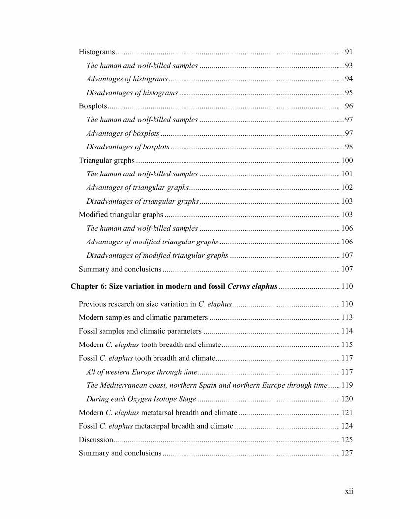
List of Tables

Table 3.1 Interobserver measurement error for tooth crown height and breadth ........... 167

Table 3.2. Eruption and wear stages recorded in this study .......................................... 167

Table 4.1 Summary of elk specimens with known ages ............................................... 168

Table 4.2 Summary of regressions of age on crown height in the known-age elk

sample ............................................................................................................. 169

Table 4.3 Summary of regressions of age on crown height the known-age white-tailed

deer sample...................................................................................................... 169

Table 4.4 Values used in the Quadratic Crown Height Method.................................... 170

Table 4.5 Comparison of regression and theoretical equations..................................... 170

Table 5.1 Model life table ........................................................................................... 171

Table 5.2 Data used to compare methods of reconstructing age distributions ............... 172

Table 5.3 Data used to describe the modified triangular graph..................................... 173

Table 5.4 Properties of the four methods for summarizing mortality profiles discussed

in this study ..................................................................................................... 174

Table 6.1 Modern specimens used in the study of size variation in C. elaphus ............. 175

Table 6.2 Climate data for the locations of the modern comparative specimens used

to investigate the relationship between C. elaphus size and climate.................. 176

Table 6.3 The relationship between M1 tooth breadth and climate ............................... 178

Table 6.4 Data on Late Pleistocene red deer M1 breadths for studying size variation ... 179

Table 6.5 Comparisons of M1 breadth by Oxygen Isotope Stage.................................. 181

Table 6.6 The relationship between metatarsal breadth and climate ............................. 182

Table 6.7 Data on Late Pleistocene red deer metacarpal breadths for studying the

relationship between size and climate .............................................................. 183

Table 7.1 First analysis: Individual samples with more than twenty-five measurable

dP4s and M1s ................................................................................................... 184

Table 7.2 First analysis: Results of the Kolmogorov-Smirnov test for individual

samples with more than twenty-five measurable dP4s and M1s......................... 185

xvi

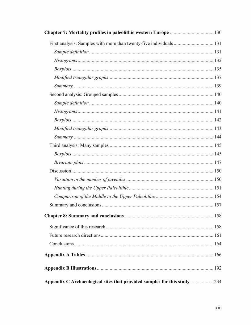
Table 7.3 First analysis: Summary statistics for the modified triangular graphs for the

individual samples. .......................................................................................... 186

Table 7.4 Second analysis: Grouped samples with more than twenty-five measurable

dP4s and M1s ................................................................................................... 187

Table 7.5 Second analysis: Results of the Kolmogorov-Smirnov test for grouped

samples with more than twenty-five measurable dP4s and M1s......................... 188

Table 7.6 Second analysis: Summary statistics for the modified triangular graph for

the grouped samples ........................................................................................ 189

Table 7.7 Third analysis: Grouped samples with ten or more measurable M1 crown

heights ............................................................................................................. 190

Table 7.8 Third analysis: Individual samples with ten or more measurable M1 crown

heights ............................................................................................................. 191

xvii

List of Illustrations

Figure 1.1 Later Pleistocene climatic and cultural stratigraphy .................................... 193

Figure 2.1 Global distribution of C. elaphus ................................................................ 194

Figure 3.1 Map of fossil sites included in this study .................................................... 195

Figure 3.2 Dental measurements used in this study...................................................... 196

Figure 3.3 C. elaphus tooth nomenclature.................................................................... 197

Figure 3.4 Postcranial measurements used in this study............................................... 198

Figure 4.1 Regression of age on crown height for elk .................................................. 199

Figure 4.2 Regression of age on crown height for white-tailed deer ............................. 200

Figure 4.3 Comparison of wear rates between elk, white-tailed deer, and reindeer....... 201

Figure 4.4 Residuals of age predictions using the regression equations........................ 202

Figure 4.5 Differences in wear rates between male and female elk .............................. 204

Figure 4.6 Residuals of ages predicted using the Quadratic Crown Height Method...... 205

Figure 4.7 Comparisons of the two age estimation methods......................................... 206

Figure 4.8 Adjusted method for estimating age from M1s ............................................ 207

Figure 5.1 Model age structures................................................................................... 208

Figure 5.2 Differences in prey age-at-death between human and wolf hunters ............. 208

Figure 5.3 First method: Histograms ........................................................................... 209

Figure 5.4 Second method: Boxplots ........................................................................... 210

Figure 5.5 Third method: Triangular graphs ................................................................ 211

Figure 5.6 Modified triangular graphs ......................................................................... 212

Figure 5.7 The effects of sample size in modified triangular graphs............................. 213

Figure 6.1 Sexual dimorphism in C. elaphus ............................................................... 214

Figure 6.2 The relationship between M1 tooth breadth and climatic variables in

modern C. elaphus ........................................................................................... 215

Figure 6.3 The relationship between M1 tooth breadth and climatic variables in

modern C. elaphus from North America .......................................................... 216

xviii

Figure 6.4 The relationship between M1 tooth breadth and climatic variables in

modern C. elaphus from western Europe ......................................................... 217

Figure 6.5 The relationship between tooth breadth and glacial/interglacial climates

in fossil red deer .............................................................................................. 218

Figure 6.6 The relationship between fossil red deer tooth breadth and

glacial/interglacial climates in various regions of western Europe.................... 219

Figure 6.7 Variation in fossil red deer M1 breadth during different Oxygen Isotope

Stages .............................................................................................................. 220

Figure 6.8 The relationship between distal metatarsal breadth and climatic variables

in modern C. elaphus from North America ...................................................... 221

Figure 6.9 Variation in fossil red deer distal metacarpal breadth during different

Oxygen Isotope Stages..................................................................................... 222

Figure 7.1 First analysis: Histograms of individual samples......................................... 223

Figure 7.2 First analysis: Boxplots of individual samples ............................................ 224

Figure 7.3 First analysis: Boxplots of individual samples ............................................ 225

Figure 7.4 First analysis: Modified triangular graphs of individual samples................. 226

Figure 7.5 Second analysis: Histograms of grouped samples ....................................... 227

Figure 7.6 Second analysis: Boxplots of grouped samples ........................................... 228

Figure 7.7 Second analysis: Boxplots of grouped samples ........................................... 229

Figure 7.8 Second analysis: Modified triangular graphs of grouped samples................ 230

Figure 7.9 Third analysis: Boxplots of small grouped samples..................................... 231

Figure 7.10 Third analysis: Bivariate plot of median crown height by time.................. 232

Figure 7.11 Third analysis: Bivariate plots of median crown height by environment.... 233

1

Chapter 1: Introduction, background, and research objectives

Fossil hominid morphology, archaeology, and genetics all indicate that

anatomically and behaviorally modern humans (Homo sapiens sapiens) originated about

50,000 years ago (kya), most likely in East Africa. These modern humans spread out of

Africa, populated western Asia, Europe, and the Far East, and eventually reached

Australia and the Americas. In this range expansion, they appear to have replaced the

archaic people who preceded them. The evidence for replacement is clearest in Europe,

where the paleoanthropological record documents that 30-40 kya modern humans and

their Upper Paleolithic industries replaced the archaic people of Eurasia, the Neandertals

(Homo neanderthalensis or H. sapiens neanderthalensis), and their Middle Paleolithic

industries (as summarized in Klein, 1999; Mellars, 1996; Stringer & Gamble, 1993).

Excavations in western Europe have been ongoing for the past 150 years, providing a rich

fossil and archaeological record, including genetic sequences from ancient Neandertals,

that allows the exploration of the fate of the Neandertals.

The Neandertals persisted through many climatic changes for hundreds of

thousands of years, yet they were replaced by modern humans in a few thousand years.

Although the fate of the Neandertals has captured the attention of paleoanthropologists

for generations, researchers still are trying to determine how and why neandertals were

replaced. One hypothesis is that modern humans were able to acquire more resources

from the environment than the Neandertals. More calories could have allowed the

modern humans to have increased fertility and survivorship (Kaplan & Hill, 1992), and

2

therefore, increased population sizes or densities, which in turn could have lead to the

continuation of modern humans and not Neandertals. The goal of this research is to

examine the similarities and differences in the hunting strategies of Neandertals and early

modern humans in an effort to understand how they extracted resources from their

environment. This study asks the question: Were modern humans better big game hunters

than Neandertals? From this research, I hope to contribute data addressing why

Neandertals ultimately went extinct and, therefore, provide a better understanding of the

pattern of human evolution.

The Neandertals

Since the first recognition of Neandertals in 1856, much of the research into

human prehistory has focused on the fate of these ancient people. Neandertals are a

distinct group of archaic humans that inhabited Europe and western Asia from

approximately Oxygen Isotope Stage 6 (OIS; Figure 1.1) until 30-40 kya. Their remains

are documented throughout western Europe; in southern central Europe; in the Caucasus

Mountains and Crimea of southern European Russia; in western Asia in what is today

Iran, Iraq, Israel, Syria, and Turkey; and as far east as Uzbekistan (Klein, 1999).

The earliest well-documented hominids found in western Europe are specimens of

H. antecessor from the Gran Dolina, Atapuerca, Spain and are from just over 780 kya

(Falgueres et al., 1999). However, Europe was continuously occupied by hominids only

after about 500 kya, as shown by the marked increase in well-supported sites after this

time (Roebroeks, 2001). From 500 kya until their demise 30-40 kya, these archaic

humans in Europe accumulated morphological features that distinguish them from all

other Old World populations. Hublin (1998) formulated this trend into the “accretion

3

model” where the Neandertal’s unique morphology resulted from an accretion process

driven by population crashes and expansions caused by Pleistocene glacial cycles. By 74

kya, the Neandertals acquired their characteristic “classic” skeletal morphology: long,

low brain cases that end with a bun on the back of the head; receding foreheads with

large browridges and protruding faces; mandibles lacking chins with large spaces behind

the third molars; and short, robust limb bones. These “classic” specimens were the first

described and are the most abundant in the fossil record, so the name Neandertal

primarily applies to specimens from OIS 3-5. European hominid fossils pre-dating OIS 6

are commonly considered H. heidelbergensis, but their taxonomic status really remains

unresolved (Hublin, 1998; Klein, 1999).

Throughout their geographic range, Neandertals most frequently are associated

with the Mousterian stone tool industry, which defines the Middle Paleolithic of Europe,

the Near East, and northern Africa. The Mousterian likely evolved out of local Acheulean

industries during OIS 6 or 7 (130-244 kya, Klein, 1999:408). The Mousterian contains a

variety of tools, such as points, side scrapers, denticulates, backed knives, and used

flakes, and it is distinguished from the preceding Acheulean by lacking large hand axes.

Microscopic and chemical analyses of lithic artifacts from the Near East show that some

of these tools were hafted and that they were used on wood, flesh, bone, and hide (Boëda

et al., 1996; Shea, 1989). While Neandertals were fully capable flint-knappers, their tools

were highly variable and are difficult to classify into discrete categories. However, some

unique variations existed during the Middle Paleolithic, such as the stemmed points that

distinguish the Aterian (e.g. Tixier, 1967). Within the Mousterian, there is little evidence

4

that Neandertals regularly worked antler, bone, or ivory into formal tools or art items,

such as figurines, pendants, or beads.

There is no evidence that Neandertals had bows and arrows or spear throwers, but

three 400-ky-old wooden spears from Germany provide some evidence of ancient

hunting technology and wood-working (Thieme, 1997). All three spears have a similar

shape of being approximately 2 m long, having maximum weight at the end sharpened to

a point, and being long and tapered at the opposite end. This morphology resembles

modern javelins, and therefore Thieme (1997) concludes that the spears were for

throwing and not thrusting. Polish and mastic residue on stone tool surfaces and impact

fractures on stone tool tips suggest that Middle Paleolithic people living in the Near East

mounted points, usually made with the Levallois technique, onto shafts to make thrusting

spears (Shea, 1989; Shea, 1998; Shea et al., 2001). These thrusting spears would have

been used at a close range, perhaps after an animal had been captured in a pit-trap or

surround, but the wound caused by the stone point likely would have disabled the prey

adequately.

Modern human origins

During much of the mid-20th century, paleoanthropologists debated the general

pattern of modern human origins, and consequently the relationship of Neandertals to

modern humans. Discussion centered on two alternate hypotheses for the overall pattern

of human evolution: Multiregional Evolution and Out of Africa. The Multiregional

Evolution model postulates that after an initial expansion out of Africa 1 to 1.8 million

years ago, H. erectus colonized eastern Asia and eventually Europe. Once in place, these

populations remained one species through gene flow and each eventually evolved into

5

behaviorally and morphologically fully modern H. sapiens sapiens, although not

necessarily simultaneously (e.g. Wolpoff, 1989; Wolpoff et al., 2000; Wolpoff et al.,

1984). In this model, Neandertals are designated as a subspecies, H. sapiens

neanderthalensis, and as such they either evolved in situ into modern humans or were

capable of interbreeding with fully modern humans arriving into Europe, although they

did not necessarily do so (Wolpoff et al., 2000). The proponents of this model suggest

that Neandertals and modern humans shared many skeletal features and were part of one

population that continued through time in western Europe (Frayer, 1992), central Europe

(Wolpoff et al., 2001), and Israel (Kramer et al., 2001). Under this model, Neandertals

would be capable of the same behaviors that are characteristic of modern humans.

The Out of Africa model also begins with H. erectus leaving Africa 1 to 1.8

million years ago, but in this model, fully modern H. sapiens sapiens did not originate

until 50-60 kya and only in Africa. They subsequently spread out of Africa and into Asia

and Europe, replacing the archaic hominids already living in these areas (e.g. Klein,

1999; Klein, 2000a; Lahr & Foley, 1998; Stringer & Andrews, 1988; Stringer & Gamble,

1993). The Out of Africa Model was formulated from fossil hominid (Bräuer, 1989;

Rightmire, 1989) and archaeological data (Klein, 1992), but genetic studies greatly

advanced the idea (Cann et al., 1987; Vigilant et al., 1991). The genetic, fossil, and

archaeological evidence for this model is clearest in western Europe, where data strongly

suggest that modern humans replaced the Neandertals by 30-40 kya. A complete

replacement means that Neandertals did not contribute significantly to the modern human

gene pool, and thus they would be considered a separate species, H. neanderthalensis.

Some intermediate models do allow for higher levels of interbreeding (Bräuer, 1989).

6

Duarte et al. (1999) recently suggested that the remains of a 4-year-old child buried 24.5

kya in what is now Portugal show evidence of hybridization because of their mosaic of

supposed-Neandertal and modern skeletal features, but others have questioned the

interpretation of the remains (Tattersal & Schwartz, 1999). The Out of Africa model has

gained the support of most paleoanthropologists, and some form of it is likely the most

accurate reconstruction of modern human origins.

The evidence for replacement

Morphology

In Europe, hominid fossil morphology abruptly changes from Neandertal to

anatomically modern humans 30-40 kya, indicating a replacement of populations and not

a gradual transition of Neandertal to modern morphology. Modern human crania look

quite different from Neandertal crania, because they have vertical foreheads; rounded

braincases; small to absent browridges; faces that are tucked under their braincases; no

spaces behind the mandible’s third molar; and prominent chins (Klein, 1999). Fossil

remains older than 30-40 kya have Neandertal characteristics, while those after 30-40 kya

resemble modern humans, indicating a population replacement. Frayer (1992) identified

cranial features that appeared in both Neandertals and modern humans in Europe, and he

used these features to argue for population continuity. When Lahr (1994) studied all Old

World populations, she found that cranial features used to argue for continuity frequently

occur, often in high incidences, outside of the regions where they are expected, and

therefore the continuity of features described by Frayer (1992) could be due to chance.

Before these features can be used to determine phylogeny, researchers must be sure that

7

they are homologous between Neandertals and modern humans (Lieberman et al., 2000)

and that they are genetically and not functionally determined (Moran & Chamberlain,

1997).

Limb-proportions provide strong support for the replacement of Neandertals by

modern humans. Neandertals, who lived in glacial Europe, had body proportions that are

characteristic of recent modern humans living in cold environments. The modern humans

that replaced the Neandertal had significantly different limb proportions, ones that are

characteristic of people living in warm environments, providing an indication of the early

modern humans’ African origin (Holliday, 1997; Trinkaus, 1981).

The human paleontological record shows that the transition from archaic to

modern morphology is visible only in Africa, and fossils with features unique to modern

humans appear approximately 127 kya (Bräuer, 1989; Rightmire, 1989). Rightmire

(1976) recognized the Middle and Late Pleistocene hominid fossils from Africa as being

distinct from the Neandertals, and Hublin (1998) documented a gradual accumulation in

Europe of unique Neandertal cranial features that distinguish the Neandertals from their

African contemporaries and modern humans. Hominid fossils document the African

origin of anatomically modern humans, and fully modern human morphology does not

appear outside of Africa until after 50 kya.

Archaeology

By at least 32-35 kya, the stone tools of western Europe exhibit a distinct change

(Mellars, 1999), and a new industry called the Aurignacian appears, which marks the

beginning of the Upper Paleolithic in Europe. Mellars (1996:393-400) characterizes the

Aurignacian as having the following: more sophisticated technology for making blades (=

8

flakes that are twice as long as they are wide); new forms of stone tools that can be

classified into types easily, including end-scrapers and burins; bone, antler, and ivory

fashioned into tools, including the Aurignacian “index fossil” – split-base points;

personal ornaments, art, and decoration; and expanded distribution and trading networks.

Early Upper Paleolithic people made a much higher percentage of their stone tools on

exotic raw materials, while Neandertals primarily used local sources to make their

Mousterian industry (Mellars, 1996). Whether the stone reached the site through the

movements of the people who lived in the site or through trade is not yet known, but the

evidence indicates that Middle and Upper Paleolithic people differed in their settlement

patterns, social organization, or both (Klein, 1999:449).

Only about a dozen of the earliest Aurignacian assemblages in Europe have

yielded human fossil remains, but where they are found, the fossils show traits that are

undeniably characteristic of modern human morphology (Churchill & Smith, 2000;

Gambier, 1989). Hoffecker (1999) also concluded that the earliest Upper Paleolithic in

eastern Europe, which was different from the Aurignacian of western Europe, is

associated only with modern humans. Neandertals have been associated with early Upper

Paleolithic industries in Vindija Cave, Croatia (Karavanic & Smith, 1998), but d’Errico et

al. (1998) question the integrity of this assemblage. The weight of the evidence suggests

that anatomically modern humans are associated with the Aurignacian.

Most archaeologists support the model that modern humans and the Aurignacian

dispersed concurrently across Europe, providing evidence of replacement of Neandertals

by modern humans instead of an in situ evolution of Neandertals into modern humans.

Mellars (1996:405-411) offers these lines of evidence for the colonization of one

9

population: the Aurignacian industry is remarkably uniform across western Europe and

very distinct from the preceding Mousterian industries; there is scant evidence for an in

situ evolution of the industry; and the industry shows unique inventions in stone, bone,

and antler working and symbolism that are unlikely to be independent inventions. While

the chronology is not fully worked out, the Aurignacian industry appeared in temporal

clines across Europe (Bar-Yosef, 2000; Bocquet-Appel & Demars, 2000a; Mellars,

1996:410; Zilhão & d'Errico, 1999). Bar-Yosef (see also Ambrose, 1998; 2000;

Hoffecker, 1999; Kuhn et al., 2001) documented an east-west trend in the earliest

appearance of Upper Paleolithic industries which began in east Africa approximately 50

kya, exited northeastern Africa 47-45 kya, entered the region east of the Mediterranean

38-45 kya, moved north into eastern and central Europe 40 kya where they diversified,

and finally appeared as the characteristic Aurignacian in western Europe 36-41 kya.

While most researchers agree with this characterization, some scholars find evidence for

continuity between Mousterian and Aurignacian stone tools and a lack of uniformity in

the earliest Aurignacian, indicating in situ evolution of the Aurignacian from the local

Mousterian (Cabrera et al., 2000).

Genetics

The genetic evidence that emerged in the past two decades provides the strongest

evidence for the replacement of the Neandertals in western Europe and an Out of Africa

model for modern human origins. Although analyses of mitochondrial DNA sequences

supplied the earliest clear evidence of a recent common origin in Africa for all living

humans (Cann et al., 1987; Vigilant et al., 1991), more recent studies of Y chromosome

sequences provided the most concordant evidence. Y chromosome variation shows that

10

the genetic diversity in people living outside of Africa is a subset of the diversity within

Africa (Underhill et al., 2001; Underhill et al., 2000), and a sample of 43 Y chromosome

sequences coalesce about 59 kya (with a 95% confidence interval of 40-140 kya),

suggesting that Y chromosomes in living men share a common ancestor that lived at this

time (Thomson et al., 2000). Estimates of the ages of certain Y chromosome mutations

suggest that people migrated out of Africa approximately 47 kya (with a 95% confidence

interval of 35-89 kya; Thomson et al., 2000). Although the confidence intervals around

these dates are large, it is important that they are in tens of thousands of years and not

hundreds of thousands of years. Further sampling of 12,000 Y chromosomes focusing on

East Asia show no evidence of contributions from archaic humans in living men,

disputing Multiregional Evolution in the area where the morphological evidence is

strongest (Ke et al., 2001). Recent mitochondrial DNA data show a concordant pattern of

high genetic diversity within Africa, coalesce about 52 (±27.5) kya, and show an

expansion out of Africa approximately 38.5 kya (Ingman et al., 2000). Autosomal DNA

evidence provides further support by showing a low level of sequence divergence,

particularly outside of Africa, which suggests a recent origin of all living people and no

significant genetic contributions from pre-modern-human populations (Knight et al.,

1996; Tishkoff et al., 1996).

In addition, short sequences of ancient mitochondrial DNA have been extracted

from multiple Neandertal fossils (Krings et al., 2000; Krings et al., 1999; Krings et al.,

1997; Ovchinnikov et al., 2000). These sequences are similar to each other and different

from all living humans, and they coalesce with modern lineages about 465 kya, with a

95% confidence interval of 317-741 kya (Krings et al., 1999). While these data do not

11

necessarily indicate a complete replacement (Nordborg, 1998), they suggest that

Neandertals and modern humans were potentially two separate lineages during the

Middle Pleistocene.

Evidence against a complete replacement

One complication to the Out of Africa model is evidence that Neandertals

performed some of the behaviors that are characteristic of Upper Paleolithic people

(Klein, 1995; Klein, 1999; Klein, 2000a). A handful of assemblages exist in central and

southwestern France and northern Spain that contain typical Mousterian tools, side-

scrapers, notches, and denticulates, but they also have unique knives, end-scrapers, and

burins that are characteristic of the Aurignacian (Harrold, 1989). The assemblages are

characterized by curved, steeply backed knives called Châtelperron points, so they are

collectively know as the Châtelperronian industry. One assemblage, Grotte du Renne,

Arcy-sur-Cure in north-central France, also contains worked bone and ivory and personal

ornaments of pierced animal teeth and ivory rings (d'Errico et al., 1998; Hublin et al.,

1996). These features make the Châtelperronian industry an Upper Paleolithic industry,

but in two sites, Saint-Césaire and Grotte du Renne, the assemblages have been firmly

linked to Neandertal remains (Hublin et al., 1996; Lévêque & Vandermeersch, 1980).

The Saint-Césaire assemblage has been dated using thermoluminescence to 36.3 ± 2.7

kya, and the Grotte du Renne was radiocarbon dated to approximately 33.5 kya, which

makes these Neandertals among the youngest known, acknowledging that the

radiocarbon date is uncalibrated and probably a minimum age (Mercier et al., 1993).

These dates overlap with the earliest Aurignacian in the area (Zilhão & d'Errico, 1999),

and researchers are still trying to determine if the earliest Châtelperronian industries pre-

12

date the earliest Aurignacian in the same areas (d'Errico et al., 1998; Mellars, 1999;

Mellars, 2000; Zilhão & d'Errico, 1999). Similar industries with unique tools, but no

ornaments, have been identified in Italy as the Uluzzian and in eastern Europe as the

Szeletian, but questions about their significance remain (Mellars, 1989; Mellars, 1996).

Currently, there are two hypotheses to explain the early Upper Paleolithic

assemblages that were manufactured by Neanderthals (d'Errico et al., 1998). The

Neandertals were either in the process of their own Middle to Upper Paleolithic transition

when modern humans arrived (d'Errico et al., 1998; Rigaud, 2000) or copied the

behaviors from modern humans in a form of acculturation (Mellars, 1999; Mellars, 2000;

Stringer & Gamble, 1993). Another possibility is that the Neandertals developed the

Châtelperronian independently, but in response to the arriving modern humans. This is an

active area of current research, and resolving the issue is dependent on refining the

chronology of the region. Given that the Châtelperronian and Aurignacian potentially co-

occur for only a few thousand years and the margins of error around all the dating

techniques, this will be a difficult task. Once the sequence of events is adequately

determined, researchers may meaningfully ask what these Upper Paleolithic-like

behaviors seen in Neandertals indicate about Neandertal cognitive ability and social

systems.

The origins of modern behavior

Assessing Neandertal cognitive capabilities is critical for understanding the

origins of modern human behavior. While most paleoanthropologists agree that

anatomically and behaviorally modern humans left Africa approximately 50 kya, recent

research has focused on the events preceding 50 kya in Africa that lead to this geographic

13

expansion. Two alternative scenarios are being discussed. The first, described most fully

by McBrearty and Brooks (see also Deacon, 1989; Henshilwood et al., 2001;

Henshilwood et al., 2002; 2000) argues that modern behaviors appeared incrementally

during the Middle Stone Age (MSA, the African equivalent of the Middle Paleolithic)

from the need to have novel solutions to problems resulting from population growth and

environmental deterioration, and therefore McBrearty and Brooks extend the roots for

modern human behavior back to the earliest appearance of the MSA, about 250-300 kya.

The features that they identify as indicative of modern human behavior include

(McBrearty & Brooks, 2000:530): blade manufacture, use of grindstones, pigment

processing, stone points, consumption of shellfish, long distance exchange, fishing,

working bone into tools, manufacturing barbed points, mining, incised pieces, microliths,

beads, and images. These new behaviors continued to lead to new technologies and

increased long-distance exchange, which in turn resulted in increased survivorship and

population growth. One difficulty with this model is that the Middle Paleolithic

Neandertals were also doing many of the “modern” behaviors that McBrearty and Brooks

identified in the MSA (d'Errico et al., 2002; d'Errico & Soressi, 2002), and some

Neandertals were able to make the Upper Paleolithic Châtelperronian. The fact that the

Mousterian and MSA people were behaving similarly and the Neandertals were replaced

argues for a more recent origin of modern humans. It also suggests that the behaviors

identified by McBrearty and Brooks (2000) as modern are not actually diagnostic of

modern humans.

The alternate view to a gradual accumulation of modern behaviors during the

MSA is that all truly modern behaviors originated simultaneously in Africa

14

approximately 50 kya. This “behavioral revolution” allowed these fully modern humans

to spread throughout the world and replace the archaic people, including the

contemporaneous non-modern MSA people (Klein, 1999; Klein, 2000a; Mellars, 1996;

Stringer & Gamble, 1993). The challenge with this model is to explain the sudden and

simultaneous appearance of all these behavioral traits. Most explanations are vague and

often postulate changes in population density, social organization or language (Gamble,

1999:350; Mellars, 1996:419; Tattersal, 2001). Klein (1999; 2000a) hypothesized that a

significant cognitive change, the product of a genetic mutation, could have caused the

behavioral revolution by promoting the ability to innovate, thus behavior could rapidly

change; this would be the origin of modern human capacity for culture. This ability to

innovate would have conveyed such an advantage that modern human population size

grew rapidly, and modern humans subsequently left Africa.

How did this replacement occur?

The current paleoanthropological evidence implies that fully modern humans and

their Upper Paleolithic tool industries were able to replace Neandertals in Europe 30-40

kya. The question remains, how did this replacement occur? What advantage did the

modern humans have over Neandertals? One possible explanation is that modern humans

were able to extract more resources from the environment. This may have allowed them

to support larger population sizes and densities.

Evidence for and against differences in resource extraction

Middle Paleolithic archaeological assemblages are notably devoid of botanical

remains, although there is sparse evidence of residues on stone tools that indicate that

15

Neandertals were exploiting plants (Hardy et al., 2001). Thus, discussions of

Neandertals’ ability to extract resources must focus on acquiring meat. The first

comparison of Middle and Upper Paleolithic large mammal exploitation in Europe must

address to what degree Neandertals were hunting or scavenging. Binford (1985; 1988)

proposed that early Neandertals from the Mousterian assemblage of Couche VIII, Grotte

Vaufrey in southwestern France (OIS 6 or 7) were scavengers, while the later Neandertals

from Combe-Grenal, also in southwestern France (OIS 4 and 5), were competent hunters.

His argument for scavenging was based on carnivore-chew versus human-cut marks,

bone breakage patterns, skeletal part representation, mortality profiles, and the horizontal

distribution of the remains. Based on sites from west-central Italy, Stiner made similar

arguments that earlier Neandertals (older than approximately 45 kya) scavenged more

while later Neandertals hunted more, because the earlier assemblages had higher

proportions of old prey and head and foot skeletal parts than the more recent assemblages

(Stiner, 1990; Stiner, 1994).

Grayson and Delpech (1994) carefully reanalyzed Binford’s data, along with their

own data on the Couche VIII fauna, in light of Binford’s research, and they firmly refuted

his proposal. They found many more stone-tool cut marks, including disarticulation and

filleting marks, than Binford identified. They also found that his own skeletal part

representation data and spatial distribution data did not support his arguments for

Neandertal scavenging. Grayson and Delpech’s research suggests that Neandertals were

capable hunters who regularly captured large game.

Subsequent scholars have also systematically investigated the possibility of

consistent scavenging in Middle Paleolithic assemblages, but they conclude that

16

Neandertals were most likely able to regularly hunt large game (Chase, 1986; Chase,

1989; Marean, 1998; Marean & Kim, 1998; Speth & Tchernov, 1998; Stiner, 1990;

Stiner, 1991a; Stiner, 1991b). This is not to say that Neandertals never scavenged.

Occasional scavenging is not necessarily an indicator of ineffective foraging, and

contemporary hunter-gatherers steal carcasses from other predators when given the

opportunity (O'Connell et al., 1988).

Middle Paleolithic assemblages across Europe contain a variety of prey, including

red deer (Cervus elaphus), reindeer (Rangifer tarandus), fallow deer (Dama dama), roe

deer (Capreolus capreolus), horses (Equus caballus, E. hydruntinus), ibex (Capra ibex),

bison (Bison priscus), and aurochs (Bos primigenius). Early studies by Mellars’ (1973;

1982) found that Upper Paleolithic assemblages in southwestern France were usually

dominated by one species, reindeer. He proposed that specialization in hunting one game

species was characteristic of the Upper Paleolithic and, therefore, modern human

behavior. Subsequent studies have shown that the proportion of sites with a great

abundance of one species does not differ between the Middle and Upper Paleolithic in

southwestern France (Grayson & Delpech, 2002) or Europe as a whole (Chase, 1989;

Gamble, 1999:235, 340-341), so specialized hunting does not distinguish Upper from

Middle Paleolithic hunting.

Ungulate species abundance in both Middle and Upper Paleolithic assemblages

apparently reflects the local environment at the time of deposition and not the prey choice

of the occupants (Chase, 1989; Grayson & Delpech, 1998; Grayson et al., 2001; Klein,

1999:453; Stiner, 1994). Mellars (1973; 1982) formed his hypothesis of reindeer

specialization using data from southwestern France. But this region experienced dramatic

17

climatic changes during the Late Pleistocene (van Andel & Tzedakis, 1996), and the

faunal community changed in response. Bordes and Prat (1965) demonstrated that in the

Middle Paleolithic sequences from Combe-Grenal in southwestern France, red deer and

reindeer fluctuated in direct response to the glacial cycles with more red deer in the warm

phases and more reindeer during the cold periods. During the Upper Paleolithic of

southwestern France, reindeer abundance increased with decreasing temperatures during

OIS 3 and 2 leading up to the Last Glacial Maximum (Grayson et al., 2001). This trend

culminated in the Magdalenian “Age of the Reindeer” just subsequent to the Last Glacial

Maximum (c.a. 18 kya). In conclusion, the abundance of reindeer in Upper Paleolithic

assemblages, when it happens, is most parsimoniously explained by increasing reindeer

abundance as a result of decreasing summer temperatures and not by intentional

specialization in reindeer hunting by modern humans (Grayson et al., 2001).

Many Mousterian sites have a high abundance of one species, and sites dominated

by steppe bison and aurochs have received a great deal of attention, likely because of

obvious comparisons with North American bison (Bison bison) deposits (e.g. Speth,

1997). The large bovids in these assemblages are often 85-99% of the ungulates present

(Gamble, 1999:235, 340-341; Jaubert & Brugal, 1990). While there are only about ten of

these sites, they have a wide geographic distribution spanning southwestern and northern

France, Germany, and the northern Caucasus (Gaudzinski, 1995; Gaudzinski, 1996).

These sites are earlier assemblages, mostly from 190-60 kya, and they are predominately

open-air deposits, often along river valleys or in sinkholes (Gaudzinski, 1995; Hoffecker

et al., 1991; Jaubert & Brugal, 1990). The composition of the deposits suggests that a few

animals were killed at the site during each hunting episode, and that the sites were

18

repeatedly used for hundreds of years (Farizy et al., 1994; Gaudzinski, 1995; Hoffecker

et al., 1991; Jaubert & Brugal, 1990). There is an abundance of prime adult animals in all

of the systematically analyzed assemblages, although the number of juvenile remains

varies, possibly biased by pre- and post-depositional destruction and excavation

techniques (Brugal & David, 1993; Farizy et al., 1994; Gaudzinski, 1995; Hoffecker et

al., 1991; Jaubert & Brugal, 1990). This suggests that small herds, possibly family

groups, may have been trapped at once. Killing just a few large bovids at once would

generate large amounts of meat, yet there is no evidence of food storage during the

Middle Paleolithic (Gamble, 1999:230). Meat could have been dried, however, and leave

little archaeological evidence. The abundance of bones at these sites indicates that even

early Neandertals were quite capable hunters, and the geographic positioning of the

deposits suggests that the Neandertals were exploiting the species’ natural movements

and the local topography to hunt game. The extent to which these sites were exclusively

kill sites or habitation sites is unknown. If they are only kill sites, then the extent to which

the Neandertals exploited other species also remains unknown; these assemblages only

indicate that the Neandertals could hunt large bovids, but do not necessarily indicate

specialization in bovid hunting.

Researchers frequently cite seasonal exploitation of faunal resources as an

indicator of hunting abilities, arguing that seasonality implies pre-planning and detailed

knowledge of the prey’s ecology. Changes in seasonality could indicate changes in land

use, resource procurement and group mobility patterns (Pike-Tay et al., 1999:284). Many

of the large deposits of large bovids show seasonal deaths. The steppe bison of Mauran in

southern France were consistently killed during the end of the summer and in autumn,

19

indicating that the animals were deposited during seasonal hunting episodes when the

animals may have been positioned on the landscape such that they were easier to capture

or drive (Farizy et al., 1994). The steppe bison deposit of Coudoulous, in southwestern

France also indicated seasonal hunting, but during the end of winter through summer with

a peak during the end of spring and beginning of summer, the likely time of steppe bison

rutting, which possibly made the animals more vulnerable (Brugal & David, 1993). The

nearby site of La Borde, dominated by aurochs, contained animals killed during all

seasons of the year (Slott-Moller, 1990). This non-seasonal hunting could be investigated

in light of differences in behavior between steppe bison and aurochs. In Cantabrian

Spain, Pike-Tay et al. (1999) demonstrated that at three sites, El Castillo, Cueva Morín,

and El Pendo, Middle Paleolithic people were seasonally targeting red deer, roe deer,

large bovids, and horse. These deposits also contained early Upper Paleolithic remains,

and the seasonal signal of hunting is the same. These data show that Neandertals were

exploiting the seasonal patterns of prey species and that they did not differ from modern

humans in this respect, but seasonality data are difficult to interpret. They need not imply

the targeting of a certain prey species during a specific season, but seasonal hunting could

be a by-product of a stationary group of humans exploiting animals that happen to be

local during only one season.

The age-at-death of prey in a faunal assemblage also provides information about

hunting abilities. Non-human predators take the youngest, oldest, and weakest members

of an ungulate herd (Carbyn, 1983; Kunkel et al., 1999; Mech, 1970; Mech et al., 1998;

Mech et al., 2001; Smith et al., 2000), while only humans are able to consistently hunt

prime adults, too (Boyd et al., 1994; Klein, 1982b; Stiner, 1990; Stiner, 1991b; Stiner,

20

1994). The hunting of healthy adult animals likely indicates that the humans used either

complex tools, such as bows and arrows or spear throwers, or built traps and surrounds

where animals of all ages were equally likely to be captured. Stiner (1990; 1994)

compared the age-at-death of cervids and aurochs in six sites in west-central Italy that

span the Middle to Upper Paleolithic transition. She found that the more ancient

Mousterian sites (older than 45 kya) contained more old prey, while the more recent

Mousterian (younger than 45 kya) and Upper Paleolithic prey ages resembled modern

hunters by containing many prime-aged individuals. Pike-Tay et al. (1999) compared

age-at-death of the cervids, equids, and large and small bovids in three northern Spanish

sites that span the Middle to Upper Paleolithic transition. They found no difference in the

ages of the animals hunted during the two time periods, and the majority of the animals

were prime adults. The Neandertals’ ability to capture prime animals is attested by the

large number of prime animals found in all of the large bovid sites discussed above

(Brugal & David, 1993; Farizy et al., 1994; Gaudzinski, 1995; Hoffecker et al., 1991;

Jaubert & Brugal, 1990). Finally, Levine (1983) studied the mortality profiles of horses in

Lower (Acheulean), Middle, and Upper Paleolithic assemblages in southwestern France.

Their mortality profiles clustered into different groups, but these groups contained

assemblages associated with all tool industries. The patterning in her data did not reflect

the chronology of the sites, and Middle and Upper Paleolithic people were taking animals

of similar ages. Most of the assemblages that she studied contained many prime adult

individuals, indicating that Neandertals were capable of obtaining prime-aged horses.

Pike-Tay (1991) studied the age-at-death of red deer in seven Upper Paleolithic

sites from southwestern France. Four were early Upper Paleolithic from the Upper

21

Perigordian (ca. 26 kya) and three were later Upper Paleolithic from the Final

Magdalenian and Azilian (ca. 11 kya). Although Pike-Tay was not studying the Middle to

Upper Paleolithic transition, her results are relevant for studying Neanderthals’ ability to

hunt. The mortality profiles from the Upper Perigordian samples contained the same

proportion of ages as a living herd, while the more recent assemblages had a bias towards

juveniles. Pike-Tay (1991:108) hypothesized that the difference was due to differences in

technology. The Magdalenian and Azilian people were hunting with spear-throwers,

which allowed individuals or small groups of hunters to take the least wary and slowest

prey, the youngest individuals. The Upper Perigordian people lacked projectile

technology, so Pike-Tay (1991:108) suggested that they used organized, cooperative

hunting to intercept and detain the prey, along with traps, snares, pits, stalking, and

ambush. She hypothesized that these strategies would take animals of different ages in

equal abundance to their presence on the landscape, and therefore there would be many

prime animals in the fossil assemblages. Based on this study, I expect that the mortality

profiles of red deer in Mousterian assemblages would more closely resemble those of the

Upper Perigordian samples, because both groups hunted without projectile technology.

This assumes that Neandertals hunted in a cooperative fashion, similar to the modern

humans. If they did not, I expect that prey mortality profiles from their sites would

resemble those accumulated by non-human carnivores.

Although there is no difference between the Middle and Upper Paleolithic in the

degree of specialization in hunting large ungulates, the proportion of taxa in faunal

assemblages does change through time. Upper Paleolithic assemblages have much higher

amounts of smaller animals in them, including fish, birds, and lagomorphs (rabbits and

22

hares; Klein, 1999:459; Stiner et al., 1999). Although all of these taxa are present in

Middle Paleolithic deposits, particularly lagomorphs, they are more abundant in later

assemblages (Chase, 1986; Stiner et al., 1999; Straus, 1977). Increased faunal diversity in

the more recent sites is mirrored in Africa where the MSA assemblages have fewer small

animals than the Late Stone Age (LSA, African equivalent of Upper Paleolithic) sites

(Klein, 1994). The ability to readily acquire fish and birds, particularly airborne species,

is significant, because hunting them required more sophisticated non-lithic technology,

such as harpoons, fish hooks, gorges, which were made out of bone and ivory, and nets.

There is no evidence for such implements in the Middle Paleolithic or MSA (Klein,

1999).

Evidence for and against differences in population density and size

Despite the apparent similarities between Neandertal and modern human hunting

strategies, the early Upper Paleolithic people must have been extracting more resources

from the environment, because they appear to have sustained denser, larger populations.

Estimating population densities and sizes using the archaeological record is notoriously

difficult; there are preservation biases against older assemblages and different settlement

patterns may generate different numbers of sites. Aurignacian sites outnumber

Mousterian sites even though the Middle Paleolithic had a much longer duration. Clark

and Straus (Clark & Straus, 1983:146) counted the number of deposits in each time

period in Cantabrian Spain; they recorded 13 Mousterian sites spanning 65,000 years or

0.2 sites per thousand years, and 18 early Upper Paleolithic sites spanning only 15,000

years or 1.2 sites per thousand years. This pattern is mirrored in southwestern France

where there are about five Upper Paleolithic sites for every one Mousterian site, and

23

again, the Mousterian spans much more time (Mellars, 1982). White (1982) criticized

analyses such as these for counting sites and not layers within sites and discussed how

different settlement systems could place sites more or less in the open-air or in rock

shelters, biasing the number of preserved and excavated sites. Even though population

density is difficult to quantify, the impression is of more people living in Europe in the

early Upper Paleolithic than in the Middle Paleolithic.

The intensity of occupation in a site provides another line of evidence for

population densities (Mellars, 1982). Mousterian caves and rock shelters appear to have

been much more ephemerally inhabited, because the density of artifacts and faunal

remains in the deposits in lower than in most Upper Paleolithic sites (although see Speth

& Tchernov, 1998 and Stiner & Tchernov, 1998 for an exception). Many Middle

Paleolithic assemblages show evidence of carnivore activity, such as carnivore remains,

coprolites, and chewing and gastric acid etching on ungulate remains, indicating that

humans did not always occupy the sites (Boyle, 1998; Speth & Tchernov, 1998). The

number of large carnivores found in Upper Paleolithic sites is greatly reduced, although

small carnivores are more abundant, possibly because they were hunted for their fur

(Klein, 1999:535-6).

The density of occupation in a region can also be inferred from the size of small

animal remains, particularly tortoises and limpets (Clark & Straus, 1983; Klein, 1998;

Klein, 2000b; Klein et al., 1999:472-3; Klein & Cruz-Uribe, 1984; Stiner et al., 2000;

Stiner et al., 1999). Both tortoises and limpets grow continuously throughout their life,

and human foragers have a natural tendency to collect the largest, therefore the oldest,

individuals. As a result, the mean age of the population decreases, and so the mean body

24

size of individuals in the population also decreases. A small mean size of a sample likely

indicates that the source population was experiencing elevated predation pressure,

although care must be taken to control for changes in paleoclimate, site function, and the

season of site use (Speth & Tchernov, 2002). Unfortunately, few known assemblages

with abundant small animals span the Middle to Upper Paleolithic transition in Europe.

The sequence of Riparo Mochi, Liguria, Italy provided a series of limpets, Patella

caerulea, in the Upper Paleolithic sequences that showed a marked size change between

19 and 24 kya (Stiner et al., 2000). The Middle Paleolithic levels in this site provided a

few specimens, and although they were too fragmented to measure, they were large,

suggesting minimal pressure on the population (Stiner et al., 2000). In the assemblages

from Nahal Meged in Israel, the mean size of tortoises (Testudo graeca) in the Middle

Paleolithic was statistically larger than the early Upper Paleolithic samples, and a similar

pattern was noted in the nearby Kebara and Hayonim Caves (Stiner et al., 2000; Stiner &

Tchernov, 1998). In both the Nahal Meged and Hayonim assemblages, the most recent

Mousterian deposits had tortoises that were similar in size to the Aurignacian deposit just

above, but their sample sizes were small. The possible effects of changes in

paleoenvironment must be carefully considered in these studies (Speth & Tchernov,

2002), but the increase in the number of small animals as well as the decrease in the size

of the small animals suggests that the earliest Upper Paleolithic people in these two

regions were harvesting these animals more intensely than during the Middle Paleolithic.

During the Middle Paleolithic, many northern regions apparently were abandoned

or sparsely populated during peak cold times, as evidenced by their lack of archaeological

sites; the Neandertals probably experienced population crashes and survived in refugia

25

(Hoffecker, 1999; Hublin, 1998). Unlike Neandertals, modern humans lived in the central

eastern European Plain during glacial times (Dolukhanov et al., 2001; Hoffecker,

1999:137). The oldest, northern-most site is possibly Mamontovaya Kurya at 66° N near

the polar Urals of Russia at the Arctic Circle and is approximately 36 kya, but the

material was in redeposited layers (Pavlov et al., 2001). Additional sites in the area are

needed to confirm this remarkable find. An incredibly rich site of Sungir’ (approximately

25-30 kya) is located at 56° N and provides firm evidence of modern humans living in

territories never previously occupied (Hoffecker, 1999). The early modern humans

moving into northern latitudes had body proportions typical of people living in Africa

today (Holliday, 1997; Trinkaus, 1981). They were able to survive under harsh conditions

because of their cultural adaptations; they built complex structures and manufactured

bone and ivory awls and needles, probably to sew clothing (Hoffecker, 1999). These

eastern European sites also provided the first evidence of systematic fur trapping (as in

Klein, 1999:535-6).

This study

Comparisons between Middle and early Upper Paleolithic subsistence strategies

and ways of life often focus on single, narrowly defined geographic regions. Differences

may be identified, but it is difficult to know if the pattern is robust when one or two sites

are considered. In this study, I wanted to assess the variation present in Middle and Upper

Paleolithic hunting practices so that I could investigate differences and similarities in

behavior between the two groups. To best control for prey behavior, I studied the hunting

of only one prey species, C. elaphus, red deer in Europe and elk or wapiti in North

26

America∗ , across space and time. C. elaphus is geographically widespread and persisted

through many climatic fluctuations. By holding the prey species constant, I can more

easily consider prey behavior, such as predator avoidance tactics, the ability to be driven,

and herd structure, in order to determine hunting strategies (Frison, 1991a). I investigate

variation in how Late Pleistocene humans hunted red deer by examining prey age-at-

death. Detailed data exist on how prey-at-death indicates hunting strategies in both

human and non-human predators, making it a good parameter for assessing variation in

hunting strategies.

Prey age-at-death as an indicator of hunting strategies

The prey choice model, as known as the diet breadth model, of Optimal Foraging

Theory guides my investigations into Late Pleistocene subsistence ecology (Kaplan &

Hill, 1992; Smith & Winterhalder, 1992; Stephens & Krebs, 1986). This model assumes

that hunters, both human and non-human, make decisions about which prey to pursue by

considering which individuals will provide the highest return rate, usually calories, per

unit of time or energy spent foraging (Stephens & Krebs, 1986). Prey availability is a

factor in this decision, because the search-time to find a certain prey is included in the

“cost” of that prey. In addition to calories, predators need to consider the risks involved

in hunting, such as the likelihood that a prey target will injure the hunter, and for humans,

the number of hunting implements that might be broken or lost. Consequently, the prey

that hunters capture informs on hunting abilities and strategies or prey choice.

∗ Throughout this study, I will refer to C. elaphus as “red deer” when I exclusively mean animals living inEurope, either in the present or during the Late Pleistocene. I will call exclusively North Americanindividuals “elk”. When I am referring to animals from both Europe and North America, I will use theircommon species name, C. elaphus.

27

For example, hunters may choose to pursue the more abundant species, the more

docile species, or the species that provides the most meat. They may also choose a

species that is more amenable to being herded or driven. The age and sex of the prey are

also potential factors influencing prey choice, because meat, marrow and organ quantity

and quality changes with age and sex, as does the vulnerability or dangerousness of the

prey. The season will affect prey choice, because migrations affect species availability

and abundance and the quantity and quality of meat, marrow, and organs. Herd structure

changes with season, so that a certain age or sex may be targeted depending on the

season. Human hunters may move beyond their fundamental caloric needs and choose

their prey based on sex, if they desire antlers for tools or trophies, or on hide quality,

which can change with age, sex or season. In sum, the behavioral ecology of each species

greatly affects a predator’s hunting strategy.

As the largest individuals of a population, adult male ungulates may provide the

most calories, but risks are involved that may make this prey unobtainable or best

avoided. These risks may dictate the hunting of more vulnerable individuals, such as the

diseased, injured, senile, or young. Consequently, age-at-death data provide information

about how readily a hunter can take the strongest or prime animals versus the weakest or

most vulnerable individuals, usually the young and old. Hunters of prime animals must

be stronger, faster, or better armed (meaning technologically sophisticated in the case of

humans) than their prey to reduce the risks of injury and increase the probability that the

animal will be taken. Cooperative hunting also increases the potential of obtaining

desirable prey.

28

Age-at-death data for prey assemblages can be acquired from field observations,

skulls of deceased wild animals, or the archaeological and fossil record. For many

species, relative prey age-at-death is readily estimated from fossil and archaeological

assemblages. Teeth continuously change throughout an individual’s life by erupting in a

predictable sequence and wearing as the animal eats, and, therefore, assessing the amount

of wear on a tooth provides a means of estimating age. Teeth also preserve well in the

archaeological record, which increases the number of assemblages that can be compared

and reduces some biases produced by post-depositional destruction. Age-at-death data

can be compiled to create frequency distributions, or mortality profiles, that show the

proportion of individuals that died in each age class. These profiles reveal one aspect of

hunting strategy by showing the proportions of juvenile, prime, and old individuals that

the predator acquired.

Objectives of this study

I have four objectives for this study:

1. Investigate the methods used to estimate the age-at-death of archaeological

specimens of C. elaphus and to construct mortality profiles for fossil assemblages. Based

on my results, I will provide recommendations for future researchers.

2. Describe variation in the age-at-death of red deer in archaeological sites

spanning the last 200,000 years in western Europe. I will investigate these data to see if

they indicate differences in hunting ability between Neandertals and early modern

humans.

3. Assess C. elaphus body-size changes through time and across space. The large

dataset that I collected for studying age-at-death also allows me to investigate the

29

relationship between climate and mean body size in C. elaphus. If I can establish a

relationship in modern populations or in fossil samples, Late Pleistocene red deer body

size will be useful as a paleoclimatic indicator.

4. Suggest directions for future research that address how modern humans were

able to replace the Neandertals. Answering this question will further the understanding of

modern human origins.

.

30

Chapter 2: C. elaphus ecology

In this study, I focus on red deer for three reasons. First, C. elaphus existed

historically throughout Eurasia and North America and was a common human prey

species whenever the two co-occurred in prehistory (Appendix C and D and Figure 2.1

and 3.1). The rich zooarchaeological record of C. elaphus facilitates comparisons

between many sites from different geographic locations and time periods. Second, C.

elaphus persists today in Europe and North America as a big game animal, so wildlife

biologists on both continents have devoted vast amounts of resources to understanding

the ecology of this species (Clutton-Brock & Albon, 1989; Clutton-Brock et al., 1982;

Houston, 1982; Murie, 1951; Thomas & Toweill, 1982). Importantly for my study, much

of this research has focused on the demographics of hunted populations to ensure that the

herds maintain viable numbers of reproductive individuals. Wildlife biologists have

collected known-age specimens to develop techniques for determining the age-at-death of

C. elaphus individuals (Brown & Chapman, 1991a; Brown & Chapman, 1991b; Hamlin

et al., 2000; Lowe, 1967; Quimby & Gaab, 1957). This makes C. elaphus one of a few

species where the relationship between tooth wear and chronological age has been well

defined (Klein, 1978; Klein et al., 1983; Klein & Cruz-Uribe, 1983; Klein et al., 1981,

but see Chapter 4 for further refinements). Finally, C. elaphus body size fluctuates

through time (i.e. Dixon & Lyman, 1996; Lister, 1981; Lister, 1984; Lister, 1993;

Mariezkurrena & Altuna, 1983; Straus, 1981; Walvius, 1961) and space (i.e. Clutton-

Brock & Albon, 1983; Clutton-Brock & Albon, 1989; Clutton-Brock et al., 1982;

31

Langvatn & Albon, 1986; Lister, 1984; Walvius, 1961), indicating that the mean body

size in C. elaphus populations may be a useful environmental indicator.

Evolutionary history

The detailed research of A. M. Lister is primarily responsible for our

understanding of the evolution of Quaternary cervids in Europe, and much of the

description here is taken from his work (Lister, 1981; Lister, 1984; Lister, 1986). The

species C. elaphus, identified by the antlers’ double lower tine, is first recognized in

Europe during the Cromerian Interglacial Complex in Britain, which is probably

equivalent to OIS 13 (Schreve, 2001) and therefore approximately 475 – 505 kya

(Bradley, 1999:212). This first species is C. elaphus acornatus, so named because the

distal end of their antlers ended in a simple, two-pointed fork. By the Hoxnian

Interglacial, now correlated to OIS 11 (Schreve, 2001) between about 347 – 421 kya

(Bradley, 1999:212), red deer evolved distinctive many-pointed crowns or cups at the end

of their antlers, and this new form is C. elaphus elaphus. The potential to develop these

crowns is still present in the red deer of western Europe today, and so they also belong to

the subspecies C. elaphus elaphus, as described by Linnaeus in 1758. The oldest fossils

included in my study are from approximately 200,000 years ago, so all the fossil

specimens considered are C. elaphus elaphus.

Prat and Suire (1971) noted that red deer from the OIS 5 deposits of Combe-

Grenal in southwestern France were very small, and Guadelli (1996) described these

specimens as a new species, C. simplicidens. Their identification is primarily based on

size and tooth morphology, particularly that of the lower fourth premolar, P4. However,

P4s are variable in morphology and, therefore, are not good taxonomic indicators (Janis &

32

Lister, 1985). These small specimens also co-occur with other mammal species that are

indicative of temperate, wet forests, while the larger individuals from the site are

associated with a colder climate (OIS 4, Guadelli, 1996). Climatic, and not taxonomic,

reasons could explain the differences in body size. Until further research is conducted on

C. simplicidens, I include these specimens in my analysis as C. elaphus, although the

particular samples containing these individuals are indicated in Appendix D.

The fossil evidence for the spread of C. elaphus into North America from Eurasia

is not as clear as the evidence for their history in Europe. According to Bryant and Maser

(1982), C. elaphus first appeared in Alaska during the Illinoian glacial stage (OIS 6).

These early elk arrived across Beringia from Siberia, but were isolated in an Alaskan

refugium during this glacial period. They apparently did not disperse fully into North

America until the succeeding Sangamonian interglacial (OIS 5). Isolation during the

Wisconsin glaciation (OIS 4-2) was probably responsible for the geographic distribution

seen in elk today (Bryant & Maser, 1982). Geist (1998:186) had a contradicting view,

because he concluded that C. elaphus was rare in North America during the Illinoian and

Sangamonian and was reliably identifiable throughout North America only after 11.5

kya; he hypothesized that the species did not become abundant until the late Pleistocene

mega-faunal extinctions opened up many new niches.

Researchers agree that North American elk originally derived from Eurasian

ancestors, but the taxonomic status of the modern groups is currently in dispute.

Although considered separate species (C. elaphus in Europe and C. canadensis in North

America) since 1780, in the early 1900’s it became apparent that individuals of both

“species” introduced into New Zealand readily interbreed (Bryant & Maser, 1982). This

33

ability to interbreed warranted the two being placed into the same species in the 1950’s,

following the biological species-concept where “species are groups of interbreeding

natural populations that are reproductively isolated from other such groups” (Mayr,

1970:12). Wilson and Reeder (1993:385-386) consider all the North American and

Eurasian populations to be C. elaphus. More recent researchers claim that the New

Zealand population is not a “natural” population. Geist (1998) found the European and

North American taxa morphologically and behaviorally distinct and claimed that the

hybrid offspring have reduced fitness, such as having intermediate, therefore ineffective,

predator avoidance strategies. Viable interbreeding would mean that the offspring are

able to survive in the “natural” state, but the New Zealand hybrid offspring can only

survive in a semi-domesticated state where there are no predators. C. elaphus is

documented to freely hybridize with C. nippon where the sika deer has been introduced,

and the offspring survive so well that wildlife managers are concerned about maintaining

the integrity of local C. elaphus populations (Geist, 1998; Lister, 1984).

For my study, the exact taxonomic definition of the European and North

American groups is not important. I primarily draw upon North American elk for a

known-age sample that I use to determine the relationship between tooth crown height

and age. Red deer and elk teeth are identical except for size (personal observation). There

is no reason to suppose that the wear rates differ more between North American and

European populations than they do within the populations, although wear rates are

correlated with diet. Ideally, I would use crown height measurements on known-age

European populations, but these were not yet available to me.

34

Diet and habitat preferences

The close management of extant C. elaphus herds in both Europe and North

America offers abundant opportunities for studies of red deer habitat preferences,

population dynamics, and interactions with human and non-human predators (e.g.,

Clutton-Brock & Albon, 1989; Clutton-Brock et al., 1982; Houston, 1982; Murie, 1951;

Thomas & Toweill, 1982). From studies of living animals, researchers know that C.

elaphus is an ecologically plastic species that is adaptable to a wide range of climatic,

topographic, and vegetation zones (Markova et al., 1995; Straus, 1981). Although red

deer often are considered to be a woodland species, they actually thrive in a variety of

habitats, from mixed forests in Poland’s Bialowieza Primeval Forest to open Scottish

highlands. Geist (1998:1) described deer as filling the niche of opportunistic foraging,

and as reviewed by Straus (1981) red deer and elk eat browse, forbs, grasses, and even

seaweed. A carbon and nitrogen stable isotope study of 27 red deer remains from Paglicci

cave (32.6-13.2 kya) in southern Italy suggested that these deer were eating mainly C3

plants, or browse, in an open environment (Iacumin et al., 1997). C. elaphus digestive

anatomy and tooth morphology suggests that they are adapted to both browsing and

grazing (Clutton-Brock et al., 1982). Their range is limited more by the need to have

protection from the snow and wind than by dietary constraints, and either trees or

topographic relief can provide this protection (Lister, 1984; Straus, 1981). For this

reason, C. elaphus never dispersed to the far northern regions that are dominated by

reindeer. They can tolerate steppe environments, but not tundra. Ideal C. elaphus habitat

is probably patchy wooded areas that provide a protective forest cover and openings with

good grazing and browsing opportunities (Harpole & Lyman, 1999; Lister, 1984).

35

The fossil record for red deer is consistent with the modern, wide distribution of

red deer. Lister (1984) documented red deer remains in Britain associated with mammals

species that are characteristic of cold, open environments, such as reindeer, woolly

rhinoceros (Coelodonta antiquitatis), mammoth (Mammuthus primigenius), and horse,

but he also found them associated with warm oak forest species, such as fallow deer, and

with hippopotamus (Hippopotamus amphibius). In Britain, red deer were present, but

never abundant, during the warm interstadials and absent during glacial periods (Bordes

and Prat, 1965; Lister, 1984). As Britain warmed after the Last Glacial Maximum, red

deer became quite abundant there and were common prey of Mesolithic hunters living

approximately 9,000 years ago (Clutton-Brock & Albon, 1989; Lister, 1984). In southern

France, red deer were abundant during the warm interglacials, but during the cold stages,

they were replaced by reindeer, although never completely (Delpech, 1996). In northern

Spain, red deer were always quite abundant, even during the Last Glacial Maximum

when arboreal pollen counts were low, suggesting an open environment (Straus, 1981).

Social behavior

Modern behavioral studies provide data on how red deer herds are organized on

the landscape. The discussion below is primarily based on Clutton-Brock and colleagues’

work on red deer in Scotland (Clutton-Brock & Albon, 1989; Clutton-Brock et al., 1982)

and research on Rocky Mountain elk (Geist, 1982). Throughout most of the year, the

males are separated from the females. Geist (1982) hypothesized that this is because

females compromise forage quality and abundance by congregating into herds for

protection, while in the summer, males seek higher quality forage, singly or in groups, in

order to build up reserves for the fall rut. Observations of elk in Yellowstone National

36

Park, Wyoming contradict Geist’s hypothesis, because the open meadows were females

and their young congregate provide high quality forage, while the males are eating lower

quality forage in the forests (E. Hadly, personal communication). During the rut, herds of

one to more than twenty females are defended by a single dominant male, and this is the

only time adult males and females exist as a group. Non-harem holding males, usually

young adults and old individuals, are peripheral to the group and may challenge the

harem-holder. During the winter, stags weakened by the rut may congregate for

protection in male herds away from the females, or they may solitarily seek higher

quality forage. Old males are often alone. Males that have survived the rut with sufficient

fat stores might remain in close proximity to the females. In the spring, calving herds

consist of the adult females, their newborns, and juveniles of both sexes and are separated

from the fully adult males. For both males and females, individual party composition is

always fluid, although females have a limited territorial range and tend to associate in

mother-daughter and sister-sister groups (Clutton-Brock et al., 1982). Males leave their

maternal herd to seek mates in other territories (Clutton-Brock et al., 2002). Party size is

often small, approximately five to ten individuals, although it can reach into the

thousands depending on the environmental conditions (Boyle, 1990). There is also a

general trend for deer species living in open landscapes to congregate into larger groups

than those living in more closed habitats, likely to avoid predators, although it may also

be due to the nutritional quality of the vegetation (Clutton-Brock et al., 1982).

Throughout different C. elaphus populations, variation exists in the prevalence of

seasonal migration. McCullough (1969) argues that migrations do not occur in C.

elaphus, but the herds do have localized movements in response to local conditions. The

37

majority of seasonal movement is usually in altitude and in response to food availability

and decreasing snow cover, and therefore the animals usually move to higher elevations

in the summer (Adams, 1982). Red deer and elk are frequently found in snow as deep as

approximately 46-76 cm, but they can tolerate deeper snow if it loose and not crusted

(citations in: Adams, 1982; Lister, 1984). Insect infestation also encourages C. elaphus

herds to seek higher altitudes during summer months (Adams, 1982; Clutton-Brock et al.,

1982). Long distance migrations that are characteristic of reindeer herds are never seen in

C. elaphus.

C. elaphus seasonal behavior may affect hunting strategies in a variety of ways.

Males are often alone or in loosely associated groups seeking better forage or mates,

which makes them vulnerable to predation because of the lack of a herd help warn them

of imminent danger. Isolated males are vulnerable, because often they are older males

unable to form a harem during the rut or are prime males weakened by the rut and

seeking high quality forage to restore their reserves for the winter. Females may be more

vulnerable, because they are smaller and lack formidable antlers. However, because they

are usually in herds, at least one female will be alert and will warn the rest of the herd if

danger approaches. Females have well defined home ranges (Clutton-Brock et al., 2002;

Clutton-Brock et al., 1982), which makes them easier for hunters to locate. Their anti-

predator strategy is to stay in a group and run from disturbance (Geist, 1982), which

probably makes this species amenable to hunting by driving the animals. Frison

(1991b:261-263) finds elk to be easily confused; if a hunter can sneak in close before

startling the group, they scatter in confusion and are easier to kill. Given proper warning,

the herd runs off to safety in a tight group.

38

Calving is synchronous, and more so in higher latitudes where the growing season

is short (Geist, 1982). Newborn elk and red deer have a “hider” anti-predator strategy

where the newborn stays hidden for most of the day away from the herd while the mother

forages nearby; in the face of danger the calf freezes, while the mother assesses the

situation (Geist, 1982). This behavior may last from one to three weeks (Geist, 1982).

During this time, the calf has not fully developed its running ability, and this, along with

its small size, makes the calf very vulnerable to predation. Even once the calf is fully

mobile, the mother still flees with the calf trailing behind, leaving the juvenile very

vulnerable to predation. Shortly before the newborn calf is born, the previous year’s

offspring segregate from their mothers. The females often stay within their mother’s

group, but the males often wander on their own, seeking other males or a group of

females (Geist, 1982). These young males may be vulnerable to predation, because they

are solitary and inexperienced.

C. elaphus body size variation

As described above, C. elaphus thrive in many different habitats, so their presence

in a fossil assemblage is not a good indicator of the surrounding environment during

deposition (Lister, 1986). Throughout these different habitats, however, red deer body

size is highly variable and therefore might be a useful indicator of environment. Modern

C. elaphus adult male lean weight ranges from 110-478.6 kg (Geist, 1998:349-350), and

paleontologists have recorded significant fluctuations in fossil body size through time

(Delpech, 1983; Lister, 1981; Lister, 1993; Mariezkurrena & Altuna, 1983). Lister (1989)

has also documented decreased body size in island populations. In northern Spain, red

deer were largest during the last glaciation, and their body size has decreased to historic

39

times (Mariezkurrena & Altuna, 1983). These changes might reflect either Bergmann’s

“rule” where cold climate selects for survival of larger body sizes, or they might reflect

differences in available resources under various environmental conditions (see full

discussion in Chapter 6). Studies by Langvatn and Albon (1986) and Walvius (1961)

suggest that body size changes in response to climate related changes in available

vegetation. If the relationship between body size and certain climatic parameters can be

determined, then red deer body size might be useful as a paleoclimatic indicator.

Ethnographic examples of methods used to hunt C. elaphus

Ethnographic data collected by early explorers and ethnographers in North

America provide information on methods commonly used to hunt elk. Although never

really the dominant prey species of any Native American group, elk were hunted in small

quantities by almost every group that overlapped their range (McCabe, 1982:88). Elk

were commonly hunted only in the southern Pacific Northwest and the Columbia River

basin area, although they were still second to fish in dietary importance (McCabe,

1982:88). McCabe (1982) provides a thorough review of early accounts of elk hunting,

and what follows is a summary of his report. I excluded hunting techniques that involved

horses, dogs, or firearms.

Elk were commonly hunted with snares or pitfalls set along commonly used trails.

Nets were also used on occasion to capture an animal. Occasionally elk were driven

along these trails to ensure that an animal fell prey to the trap. Native Americans were

also able to successfully hunt elk with ambushes from blinds alongside game trails. One

hunter would chase an animal so that it passed by another hunter in hiding, and the

second hunter would then spear the animal. Deep snow and rivers were often used to

40

slow the elk so hunters could get close enough to dispatch the animals. Elk would be

chased into snow banks by hunters on snowshoes or chased into rivers, sometimes

covered by thin ice, and killed by hunters waiting in the water or in canoes. Multiple

hunters could also chase the elk to exhaustion, as well. There are a few descriptions of elk

being driven over cliffs or into surrounds, but these are rare. Single hunters or small

groups could accomplish all of these hunting methods, and there is little archaeological

evidence for large organized communal hunting, as is often seen with bison (Frison,

1987). Most hunting methods rely on elk’s natural tendency to flee from danger, and

while they do not stampede, they can be driven.

Unfortunately, each of these Native American hunting strategies is from

ethnographic documentation, and associated archaeological signatures are unknown. The

ethnographic literature does provide some information on the preferred animals:

“These Indians…concentrated on yearlings, whose meat was more tenderthan bison or older elk. Elk cows were hunted shortly after the calving season,because their hides were most pliant at that time” (as in McCabe, 1982:72).

“When there was a choice between sex and age classes of elk, the Indiansinvariably killed mature bulls. The amount of meat that an animal provided was ofparamount importance” (as in McCabe, 1982:72).

These comments confirm that age-at-death of prey in archaeological assemblages should

provide data on ancient hunting strategies. Combining this age data with sex data would

maximize information, but it is difficult to reliably reconstruct the proportions of each sex

in a fossil assemblage of red deer (Klein & Cruz-Uribe, 1994; Mariezkurrena & Altuna,

1983).

41

Chapter 3: Samples and data collection

Research samples

Modern samples

I used modern specimens of C. elaphus in multiple contexts: to compare human

and wolf hunting strategies, to refine age determination techniques, to compare different

methods for reconstructing mortality profiles, and to study body size variation. The data

for these studies came from three sources: human-hunted elk with associated known ages,

wolf-killed elk with associated cementum annuli ages, and comparative specimens from

multiple zoological collections. For comparative purposes, I also used a sample of

known-age white-tailed deer (Odocoileus virginianus), measured by C. Wolf.

The human-hunted sample is of Rocky Mountain elk (C. elaphus nelsoni) from

Montana just north of Yellowstone National Park, Wyoming. These specimens were all

marked as calves and were subsequently retrieved at hunter checkpoints, and therefore

they have known ages in months associated with them. Data on this sample were

collected twice. Quimby and Gaab (1957) accumulated the original known-age

specimens for their wear-stage study, and C. Wolf measured this sample’s tooth crown

heights in the late 1970’s with the purpose of developing a technique that could be used

to assign age to fossil C. elaphus specimens (Klein et al., 1983; Klein & Cruz-Uribe,

1983; Klein et al., 1981). In the summer of 2000 I re-examined this collection, which is

housed at Montana State University (Bozeman, Montana). I collected additional data and

compared my measurements with the Wolf’s measurements of the same specimens. In

42

addition, I collected supplementary data on known-age Rocky Mountain elk from the

same general population in Montana that were housed at the Montana Department of

Fish, Wildlife, and Parks (Bozeman, Montana). A team from this institution tagged the

specimens as calves from 1972-97 and collected the mandibles at hunter checkpoints as

part of a study comparing estimates of age using wear stages to incisor cementum annuli

counts (see Hamlin et al., 2000 for a complete description of the sample and their study).

I combined these two samples into one known-age sample (n = 226), which I used to

refine the Quadratic Crown Height Method (QCHM) for estimating age in fossil C.

elaphus (Chapter 4) and as a sample with a known age distribution to compare methods

of reconstructing mortality profiles (Chapter 5). I also used this sample to compare

patterns of sexual dimorphism (most specimens were also of known sex) and body size

variation (Chapter 6) and as an example of human hunting (Chapter 7).

The wolf-kill sample is of Rocky Mountain elk from Yellowstone National Park,

Wyoming. Since wolf (Canis lupus) reintroduction into Yellowstone in 1995 and 1996,

park biologists have been tracking the wolves as part of larger behavioral studies to

understand the new predators’ impact on the Yellowstone ecosystem. During the winter

months when snow cover makes tracking easiest, biologists collected data on each wolf

kill, including mandibles for age determination by incisor cementum annuli and

metatarsals for inferring the condition of the animal from their marrow quality (Mech et

al., 2001). The primary prey of the wolves was the local elk (Mech et al., 2001; Smith et

al., 2000). I studied the mandibles and metatarsals of the elk that were killed by wolves in

1999, the largest complete sample available at the time. D. Smith provided cementum

annuli ages from incisors for all of these specimens, and because Hamlin et al. (2000)

43

demonstrated the reliability of the cementum annuli technique in modern specimens, I

consider the cementum annuli ages to be known-ages. I used these wolf-killed elk (n =

98) as a sample with a known age distribution to compare methods of reconstructing

mortality profiles (Chapter 5) and to compare patterns of sexual dimorphism (many

specimens were of known sex) and body size variation (Chapter 6). Finally, the wolf-kill

sample provided a good comparison of how wolves and humans hunt animals of different

ages.

My third modern sample is composed of many comparative specimens from

zoology museums and zooarchaeology laboratories in the United States and western

Europe. In the United States, I collected data at the California Academy of Sciences (San

Francisco, California), Montana Department of Fish, Wildlife, and Parks (Bozeman,

Montana), Montana State University (Bozeman, Montana), Museum of Vertebrate

Zoology (Berkeley, California), National Park Service (Yellowstone National Park,

Wyoming), and the Philip L. Wright Zoological Museum (Missoula, Montana). In

Europe, I measured comparative specimens in the British Natural History Museum

(London, United Kingdom), Römisch-Germanisches Zentralmuseum (Neuwied,

Germany), Sdad. de Ciencias Aranzadi (Donostia/San Sebastián, Spain), Universität

Tübingen (Tübingen, Germany), and Université Bordeaux I (Talence Cedex, France). I

used these specimens to study sexual dimorphism and the relationship between mean

body size of a population and various environmental parameters.

Fossil samples

The 64 fossil localities used for my study are shown in Figure 3.1, with the

names, locations, excavators, where the assemblages were housed, and references for

44

each site listed in Appendix C. Appendix D provides detailed information about each

layer within each site: associated tool industry, red deer abundance by NISP, OIS, date,

and climatic data. Some data are not available for some sites and assemblages. My data

collection focused on determining the age-at-death of the specimens and taking

measurements for tooth and body size. All of the other data points, including full faunal

lists and counts, dates, and climatic information, were taken from the references listed in

Appendix C and discussions with the museum curators and site excavators.

My sampling strategy for the fossil assemblages was to pick a few large, well-

documented sites, travel to the museums that housed those collections (listed in Appendix

C), measure the red deer specimens in those collections, and then measure other red deer

available in the museum. The larger, target assemblages included Arago, Combe-Grenal,

Gabasa, La Riera, Lazaret, Piegu, and Urtiaga. R. G. Klein allowed me to use his data on

many large samples from northern Spain: Altamira, El Castillo, El Juyo, and Majolicas.

K. Cruz-Uribe provided data on the Star Carr, England sample. These large samples

formed the basis of my study on Late Pleistocene hunting by humans, and I included the

smaller samples in my study of body size changes through time and space.

Data collection

Metric data

On teeth, I measured mandibular deciduous fourth premolar (dP4), the fourth

molar (P4), and the first (M1), second (M2), and third (M3) molars, as shown in Figure

3.2.A, and the analogous maxillary teeth. I took the same measurements on isolated teeth

and teeth in their mandibles. Crown height and breadth were taken on the anterior two

45

lobes of each tooth, along with occlusal length and basal length (see Figure 3.3 for a

description of nomenclature). Following Klein and Cruz-Uribe (1984:46-47), crown

height was measured as the minimum distance between the occlusal surface and the line

separating the enamel of the crown and the dentine of the root. For mandibular teeth,

crown height was measured on the buccal-most surface; for maxillary teeth, the lingual-

most surface was measured. Tooth breadth was defined as the maximum buccolingual

dimension, and basal tooth length was the anteroposterior dimension of the tooth at the

crown base, just above the crown-root junction (Klein and Cruz-Uribe 1984:176).

Occlusal length was taken as the maximum anteroposterior length of the tooth on the

occlusal surface (Driesch, 1976:56). When complete dental rows were preserved, I

measured premolar, molar, and total row length according to von den Driesch (1976:37,

56) and Figure 3.2.B.

For a body size proxy, I measured distal metacarpal and metatarsal mediolateral

and anteroposterior diameters according to von den Driesch (1976:92), Klein and Cruz-

Uribe (1984:20) and Figure 3.4.A and B. Anteroposterior diameter was taken on the

medial condyle. When complete bones were present, I also measured maximum length

(Klein & Cruz-Uribe, 1984:20).

I took all measurements with Mitutoyo digital extended point jaw calipers (965

Corporate Blvd., Aurora IL, 60504; www.mitutoyo.com) and recorded them to the

nearest hundredth of a millimeter. I collected all data directly into a spreadsheet using a

SmartCable (7403 Lakewood Drive #14, Lakewood, WA 98499; www.smart-cable.com)

that connected the calipers to the computer. I used the DigiCal software interface (written

as shareware by Gary Rensberger and available at http://life.bio.sunysb.edu/morph/soft-

46

dataacq.html) which converted the SmartCable’s modem-like signals into text that was

inputted directly into JMP statistics software (SAS Institute Inc., JMP Software, SAS

Campus Drive, Cary, NC 27513; www.jmpdiscovery.com).

R. G. Klein provided data taken by himself on comparative and fossil material

and by C. Wolf on known-age specimens. In order to ensure that all measurements were

comparable when combining samples, I calculated the percentage of interobserver error

following White and Folkens (1991:292) for measurements that were taken both by

others and myself on the same specimens. I compared my measurements with C. Wolf’s

on the Quimby and Gaab known-age collection, and my measurements with R. G. Klein’s

on comparative material housed in the British Museum of Natural History (Table 3.1). A

pooled sample of breadth measurements on all tooth types has a mean interobserver error

of 2.5% (0.36 mm), and the error of tooth crown height measurements on the same

specimens is 2.9% (0.30 mm). These errors are small enough that data can be shared

between researchers, and they confirm the replicability of these measurements.

Non-metric data

I coded the eruption and wear stage for each tooth that I measured as shown in

Table 3.2. Stages of eruption were identified as the following: “E1” when the tooth was

still in the crypt (the bone that surrounds the growing tooth in the maxilla or mandible;

Hillson 1986:178) so that none of it had emerged above the gum line; “E2” when the

tooth was only half erupted; “E3” when the tooth was over half erupted but the cusps

were still not in occlusion; and “E4” when the tooth was in occlusion, as evidenced by

the cusps being worn, but the crown height was not measurable because the base of the

crown had not emerged above the alveolar bone. For E2-E4, I measured the tooth height

47

from the alveolar bone to the occlusal surface, although these measurements were not

included in the current analyses. When crown height was measurable, either because the

tooth was fully erupted from the mandible or it was isolated from its mandible, I coded

wear as the following: “UW” when a tooth was completely unworn; “VEW” when there

was only a very slight amount of wear on the edge of the cusp and the crown height

represented the height of an unworn tooth; “LW” when the occlusal surface has high

peaks and the dentine bands are narrow; “MW” when the occlusal peaks are muted to no

longer existent and dentine bands are wide; “HW” when the occlusal surface is flat and

the crown is more than 50% worn away; and “VHW” when the crown is completely worn

away. In C. elaphus, the crown-root junction is visible on a tooth in its mandible only

after the tooth has come into occlusion. Therefore, the stages of E3 and E4 exclusively

describe teeth in the mandible, and UW primarily identifies isolated teeth. It is very rare,

if not impossible, to obtain an unworn crown height for a tooth still in its mandible.

These wear stage data were taken primarily to supplement and confirm my

measurements, and they have had only a secondary role in the subsequent analyses. There

are two exceptions. First, the identification of the “UW” and “VEW” teeth was necessary

to determine the unworn crown height of a given sample. This measurement is used to

help estimate age-at-death, because it makes it possible to quantify the amount of wear on

other teeth from the same sample. Second, in some analyses I needed to include the total

number of dP4s present, not just the measurable teeth (meaning the tooth had erupted

enough so that the crown-root junction was visible). For these analyses, I included dP4s

coded with all eruption and wear stages.

48

I also noted any peculiarities, such as a pathology or unusual wear. Unusual teeth

were omitted from subsequent analyses if the relevant measure would be affected.

Finally, I recorded the state of epiphyseal fusion for the metapodials. All unfused

epiphyses were omitted from the analyses.

Analyses

All bivariate plots, regressions, and correlations were calculated in JMP, and all

boxplots were created in DataDesk (Data Description, Inc., P.O. Box 4555, Ithaca, NY

14852; www.datadesk.com/). R. G. Klein provided his Smirnov program to run

Kolmogorov-Smirnov tests for the histograms. As described in Chapter 5 and by Steele

and Weaver (2002), a statistical test was developed for the triangular graph as part of this

project, and T. D. Weaver wrote the Triangle program that employs the new method. The

Triangle program is available is available by contacting the author.

In my fossil analyses, I did not distinguish between right and left teeth or

metapodials. For teeth, the actual number of mandibles represented by the sample is

somewhere between the number of rights or lefts, which ever is larger, and the sum of the

two. For example, Lazaret E has 13 right M1s and 9 left M1s for a total sample of 22

measurable M1s. The minimum number of individuals present in the sample is 13, but up

to twenty-two individuals could be represented. Of course, more mandibles may have

been deposited during ancient times, but only a subset of them survived to the present.

Given the number of isolated teeth in each fossil sample, I assumed that teeth from either

side of the jaw were independent. Examination of the coefficients of variation (C.V.) in

some of my larger samples reinforces this assumption. The C.V. provides a measure of

the homogeneity of a sample. If the variance is low, the sample is more homogenous. If

49

many of the rights and lefts of my samples are from the same individuals, the C.V. of

tooth crown heights of a combined sample should be lower than the variation found in

either rights or lefts, because many of the teeth will be mirrors of each other. Fortunately,

this is not the case. For Lazaret E, the C.V. of M1 crown heights is 49.97 for the rights,

46.39 for the lefts, and 47.37 for the total sample. I performed the same comparison for

eleven of my larger samples, and the differences are always small. When the C.V.s for

the groups of right teeth are compared to the C.V.s for the total groups of teeth, there is

no significant difference (Wilcoxon test: p = 0.6694; Median test: p = 0.6770). The same

is true of the lefts (Wilcoxon test: p = 0.6936; Median test: p = 0.6770). The lack of

increased homogeneity in the combined samples of rights and lefts allows me to analyze

both rights and lefts as one sample. In my modern specimens, I measured only one

mandible, metacarpal or metatarsal for each individual, so there is no chance of counting

these individuals twice.

50

Chapter 4: Methods of age determination

Faunal analysts have long recognized that the age distribution of a species in a

sample provides data about the species’ life history patterns and the specimens’

depositional history, but assigning specimens into age classes is not always so easy.

Numerous methods exist for assessing age at death of archaeological specimens (for

reviews see Amorosi, 1989; Morris, 1972; Pike-Tay, 2000; Wilson et al., 1982), yet

epiphyseal fusion, tooth cementum annuli, and tooth eruption and wear remain the most

reliable and frequently applied methods (Klein & Cruz-Uribe, 1984; O'Connor, 2000;

Reitz & Wing, 1999). In this study I rely on measuring tooth crown heights so that I can

objectively determine the amount of wear on the tooth and perform statistical analyses on

the results. In this chapter I review previous studies on determining age in C. elaphus by

tooth eruption and wear. Using a larger sample of known-age C. elaphus, I follow Klein

et al. (1983) to re-evaluate the utility of the Quadratic Crown Height Method (QCHM) to

estimate age-at-death in fossil populations of red deer. Finally, I offer adjustments to the

theoretical quadratic formula, which I then use in my subsequent analyses.

Teeth as indicators of age

One of the primary goals of my study is to determine the ratio of prime to old

individuals. Although important for discussing juvenile to adult ratios, epiphyses are

fused once adulthood is reached and, therefore, are not useful for determining ratios of

prime to old individuals. Thus, I used teeth, which continually change throughout an

animal’s life, to estimate age-at-death of the fossil specimens. Minerals, primarily

51

hydroxyapatite, constitute 96-97% of tooth enamel (Scott & Symons 1974 as in Hillson,

1986), so teeth are more resistant than bone to organic decomposition and mechanical

erosion. Consequently, teeth are the most common mammalian fossils found. The same

tooth type (P4, M1 etc.) of different ages should preserve equally well. Unlike many post-

cranial elements, teeth are almost always identifiable to species, reducing the possibility

that a mortality profile might actually be a mix of two or more similar-sized species. Two

methods for determining animal age-at-death from teeth have received the most attention:

counting annually deposited cementum increments and assessing tooth eruption and the

degree of wear.

Studies demonstrate that age-at-death in modern C. elaphus specimens can be

successfully estimated by counting the number of seasonal bands of cementum, known as

cementum annuli, that are deposited on the roots of a tooth (Hamlin et al., 2000; Keiss,

1969; Lowe, 1967; Mitchell, 1967; Pike-Tay, 1991). Pike-Tay (1991; Pike-Tay et al.,

1999) applied this method to fossil red deer. Two types of bands are identified: “annuli”

which are narrow and dense and represent periods of slow growth corresponding to

winters, and “zones” that are wider and less dense and represent periods of rapid growth

corresponding to summer (Pike-Tay, 1995:274). The formation of these bands is

influenced by the quality of the diet and biomechanical stress resulting from mastication

(Lieberman, 1993). Because these bands are deposited seasonally, cementum annuli often

are examined to determine prey season-at-death (Burke, 1995; Lieberman & Shea, 1994;

Pike-Tay, 1991; Pike-Tay et al., 1999). To employ the method (as described by

McKinley & Burke, 2000; Pike-Tay, 1995), teeth are embedded in epoxy and cross-

sectioned down the mesial-distal midline of a molar. The exposed tooth is polished and

52

attached to a glass slide. The tooth is sectioned again parallel to the slide, and this thin

section is ground and polished to a thickness of 30-50 µm. The thin section is viewed

under polarized transmitted light, and in ungulates other than horses, the annuli are

counted on the root just below the crown-root junction. In horses, the cementum annuli

are counted on the folds of the crown, because the roots form at an advanced age

(McKinley & Burke, 2000). The amount of time represented before the cementum annuli

began to form on the adult tooth (i.e. time elapsed while the deciduous precursor was in

place) must be added to the number of annuli to obtain an estimated age-at-death.

Cementum annuli studies have their limitations. In modern specimens teeth are

often decalcified before being cross-sectioned (Hamlin et al., 2000), but fossil teeth

usually do not retain enough organic matter to survive this process (Pike-Tay, 1991:62).

Also, incisors are the most often studied element in modern specimens (as in Hamlin et

al., 2000), but they are fragile and difficult to identify when isolated in an archaeological

context. Counting cementum annuli requires specialized equipment and training to

accurately execute, which limits the method’s general utility. However, the greatest

limitation for zooarchaeologists is that this method requires large numbers of

irreplaceable fossils to be cross-sectioned to generate one mortality profile. For these

reasons, I chose to determine age in my samples by examining tooth eruption and wear.

Age determination by eruption and wear

Age can be estimated in complete mandibular rows by determining which

deciduous teeth have erupted and been shed and by evaluating the amount of wear on the

adult teeth. The premise is that teeth erupt and are replaced in a predictable and timed

sequence, and once in place, mastication wears down a tooth’s surface at a rate that is

53

related to age and diet. Investigators can estimate the degree of wear by comparing the

sample in question to known-age samples, previously sequenced samples, written

descriptions, photographs, or measurements. These can be used to assign developmental

or relative ages, but comparisons using a method based on samples with known ages are

essential for establishing chronological ages (i.e. age-at-death in months or years).

Quimby and Gaab (1957) published a pioneering study on determining the age-at-

death of C. elaphus mandibles using a known-age reference sample. Wildlife biologists

tagged newborn Rocky Mountain elk from Montana in the vicinity north of Yellowstone

National Park and collected a sample of 168 known-age mandibles. This study showed

that calves, yearlings, and 2-year olds could be assigned to age class using the state of

shedding of their deciduous teeth and eruption of their permanent teeth. Once the

complete adult dentition was in place, age was more difficult to determine and the

difficulty increased with age. This study involved comparisons of the known-age

specimens to a jaw board of specimens assigned to age by previous comparison to the

known-age specimens, determined key presence/absence characters that described each

age class, and measured tooth height from the gums to the occlusal surface. Quimby and

Gaab found that comparison to the jaw board was more accurate than comparison to

written characteristics, particularly when the specimen was older. They also found that

tooth crown heights were indicative of wear, but difficult to measure in the field on

hunters’ kills and dependent on the gum line being intact. They concluded that the best

method for determining the age of their unknown sample of elk was comparison with the

known-age mandibles. Following that was comparison to assigned-age mandibles, and

finally comparison with good drawings or photos of known-age mandibles. Not

54

surprisingly, the level of experience of the examiner also determined the accuracy of the

age assignments. Luckily, when errors occurred, they were unbiased – specimens were

equally likely to be over or under aged. One limitation of Quimby and Gaab’s study is

that although the sample was large, it was skewed toward younger individuals with only a

few specimens represented in the older age classes. The difficulty in assigning age to

older specimens might be resolved if additional older specimens with known ages were

available.

Lowe (1967) used a sample of 34 known-age Scottish red deer (C. elaphus

scoticus) mandibles from the island of Rhum, Scotland to investigate four methods of age

determination: tooth and jaw measurements; dentine increments inside the incisor crown;

annuli in cementum deposits on the root pad of M1; and tooth eruption and wear stages.

He found that comparing tooth eruption, shedding, and wear of unknown specimens to

known-age specimens was the most reliable method, although he also provided a list of

characters and photographs describing each age group. In measuring his mandibles, Lowe

found that the best age estimator was a linear function that depended on the distance

between the third molar and the posterior margin of the angular process, jaw depth below

the first molar, and the minimum crown height of the first molar. This function assigned

correct ages for half of the specimens, and with one exception, all other mandibles were

predicted within plus or minus a year. Lowe acknowledged that although individuals of

the same age often exhibit variability in crown height, maximum crown height (as

measured in my study) might actually be a better predictor of age than the minimum

crown height he measured (measured from the “saddle” of the tooth or the lowest point

between the two cusps). This is because the cusps of the tooth are actually in occlusion

55

and wearing for a period of time before the “saddle” wears (before minimum crown

height begins to record a decrease in size). Another limitation of Lowe’s study was the

small sample size and young ages of the known-age individuals. The oldest specimen is

96 months (8 years) old whereas C. elaphus individuals can live to be 192 months (16

years) and older (Houston, 1982; Lowe, 1969).

In more recent studies, Brown and Chapman developed scoring schemes for

determining the age of juvenile (Brown & Chapman, 1991a) and adult (Brown &

Chapman, 1991b) Scottish red deer mandibles. To do this, they used 113 mandibles from

Richmond Park, Surrey, England that had known ages ranging from 1 month to 138

months (11.5 years). They used X-rays of the 82 juvenile mandibles to identify stages of

tooth development and eruption, such as evidence of the crypt and degree of crown and

root formation. In total, they identified 10 juvenile stages. Each tooth in the mandibular

row was given a score that represented the stage, and all of the scores for the row were

summed so that the scores became higher as the individuals became older. The regression

equation of age on score provided a method of predicting ages (with 95% confidence

intervals) for mandibles of unknown age. Using this method, age was predicted for the

known-age juveniles to within ±4.7 months or less (Brown & Chapman, 1991a:93).

Brown and Chapman (1991b) developed a similar scoring technique for wear

features on adult dentitions (n = 111) using the same known-age Scottish red deer sample

as in their study described above. They identified 20 zones for M1 and M2, and 25 for M3.

A score of 0, 1 or 2 was given for each of these zones based on the degree of wear, and

the scores were added for the molar row. They regressed age on score to obtain a

curvilinear regression equation that they could use to predict age for unknown mandibles.

56

As scores increased with age, the width of the 95% confidence intervals also increased.

The maximum interval was ±30.5 months for the oldest individuals. Their study showed

a large range of ages during which a particular wear pattern, or overall wear pattern,

appeared in older individuals, and, therefore, they found that scoring individual features

accounted for all aspects of the wearing phenomenon by accumulating data on wear

locations. Brown and Chapman (1991b) found their method to be good because using the

scoring system increased the objectivity of recording wear patterns. It also gave a

quantified value with confidence intervals that could be used in statistical analyses,

unlike coded wear stages. The scores also accounted for variation in wear patterns of

animals with the same age. In addition, coding should reduce the need for a known-age

reference sample or jaw board to assist with accurate wear assessments, as recommended

by Quimby and Gaab (1957).

There are limitations in using tooth eruption and wear to estimate age from

mandibles of C. elaphus or any other species. One is that wear may vary from population

to population due to diet differences. This variation will affect estimates of age using

both wear stages and crown height measurements. If an animal is eating more grasses or

there is more sand and grit in the diet, the teeth may wear faster and make a specimen

look older than its chronological age. Spinage (1973:183) suggested that teeth are critical

for survival; it would be surprising if they varied widely in efficiency in a single species,

because this is how animals acquire energy. This is particularly true because consistent

wear (not too much or too little) is necessary to maintain a healthy mouth in wild

populations (Spinage, 1973). Lowe (1967) found that teeth of red deer from German

forests had similar wear per age patterns as red deer from Rhum, although the climate,

57

habitat, and management were very different. Spinage and Brown (1988) reached the

same conclusion when they studied the wear on two geographically separated subspecies

of African buffalo (Syncerus caffer) that differ in climate, diet, and body size. Important

for my study of Late Pleistocene red deer, they concluded that “tooth wear is relatively

constant within species despite wide differences in bodily size and environment”

(Spinage & Brown, 1988:227). Many of the studies cautioning differences in wear rates

between populations have included domesticated animals or other populations where, at

least for part of the year, humans supplemented the animals’ diet (Gifford-Gonzalez,

1991; Spinage, 1973:174), although the problem has also been noted in wild populations

(Flook, 1970). No one has devised a reliable method to account for differences between

populations in rates of wear, and more research is needed on this problem. For the

moment, age-at-death assessments using wear on teeth must assume a consistent rate of

wear between individuals separated in space and time.

Individual variation may also reduce the accuracy of age determination methods.

There may be variation in the ages at which teeth erupt and are shed. Chapman and

Brown’s (1991b:525) review of the literature on these ages combined with Lowe’s (1967)

and Quimby’s (1957) studies suggests that in C. elaphus, variation in the ages at which

teeth erupt is likely to be minor. Other factors, including favoring one side of the jaw, are

more likely to increase the variation within one population. Kierdorf and Becher (1997)

suggested that individual variation may be due to differences in the degree of enamel

mineralization. They recommended measuring enamel hardness along with degree of

wear, but acknowledge that this is requires specialized, expensive equipment and is labor

intensive.

58

A major limitation to using tooth eruption and wear to estimate age is that the

methods described above are best used on complete dental rows. Unfortunately, these are

rare in fossil samples, and zooarchaeologists need a method of age estimation that can be

used in the absence of a reference sample and on isolated teeth. Measuring tooth crown

heights to assess the amount of wear provides an objective, easy to replicate, non-

destructive technique that can be applied to both isolated teeth and teeth in mandibles,

making it ideal for archaeological assemblages. The interobserver error for this

measurement is low, 2.9%, thus demonstrating its replicability (Table 3.1).

The Quadratic Crown Height Method

Spinage’s model

Spinage (1971) first proposed a wear model for using crown heights to age

hypsodont ungulates. Klein and colleagues (Klein et al., 1983; Klein & Cruz-Uribe,

1983; Klein et al., 1981) tested this model on a sample of known-age elk. The technique

now is known as the Quadratic Crown Height Method (QCHM) and employs a set of

quadratic formulas based on a variable rate of wear that can be used to predict age-at-

death from tooth crown height when the beginning and end points are known. Unlike the

eruption and wear methods, the QCHM is easy to replicate, is objective, and can be

utilized with isolated teeth. Unfortunately, the method is subject to the same variations in

individual and populational wear rates as other tooth wear methods. To use these

methods, individual variation must be random, and the method must not consistently

over- or under-estimate the ages of animals (Spinage, 1973).

59

Spinage’s model (1971; 1972; 1973) is based on the observation that when crown

height is plotted against age, wear rate is not linear but actually slows with age. This may

be because, as the opposing occlusal surfaces M1 become smoother, friction decreases

and as M2 and M3 begin to wear, friction on anterior surfaces further decreases (Spinage,

1971). Although Spinage found that using known-age comparative specimens was the

most reliable way to accurately determine the age-at-death of an unknown individual, the

conceptual wear model was satisfactory in “predicting the mean age of samples, and not

the age of individuals” (Spinage, 1973:183).

The QCHM assumes that when the permanent teeth are worn completely away

(crown height equals ‘0’), the animal dies. Because M1 erupts before M2, M1 will wear to

‘0’ before M2. Ideally the age when crown height equals ‘0’ would be calculated for each

tooth from large known-age samples, but these data are unavailable for most species,

including C. elaphus. Instead, the age of potential ecological longevity must be used.

Potential ecological longevity is not the mean life span for the species, but the maximum

age that a wild individual can reasonably obtain. The QCHM formulas are (from Klein et

al., 1983:49):

For deciduous teeth: AGE = AGEs [(CH-CH0)/CH0]2

For permanent teeth: AGE = (AGEpel – AGEe) [(CH-CH0)/CH0]2 + AGEe

Equations are calculated by substituting the appropriate values for each tooth.

AGEs is the age at which the deciduous tooth is shed, AGEe is the age at which the

permanent tooth erupts, and AGEpel is the potential ecological longevity of the species.

In this study, age is measured in months. CH0 is the mean initial unworn crown height for

each tooth type for the sample under study, and CH is the crown height, measured in

millimeters, of the specimen for which age is being assigned.

60

Testing the model with known-age elk

Spinage had reasonable success with his model for assigning age in impala

(Aepyceros melampus, Spinage, 1971) and zebra (Equus burchelli boehmi, Spinage,

1972), but he lacked large samples of known-age specimens with which he could fully

test his model. Klein and colleagues (Klein et al., 1983; Klein & Cruz-Uribe, 1983; Klein

et al., 1981) tested Spinage’s wear model with Quimby and Gaab’s (1957) known-age

sample, plus a few specimens that had been added since the 1950’s. Their sample

consisted of 170 mandibles with ages ranging from 5 months to 260 months (21.7 years,

Table 4.1, Klein et al., 1983). The majority of the specimens were collected at hunter

checkpoints, so the month of death was mainly from October to January. Because Rocky

Mountain elk in this region give birth around June 1st each year, the specimens formed

discrete clusters around the half-year mark. Until 5.5 years, the sample was an even mix

of males and females, however, after this age, the sample was primarily females and

“unknowns” that were probably males whose antlers were removed (Klein et al., 1983).

Although, the oldest individual was 260 months (21.7 years) old, 90% of the sample was

younger than 72 months (6 years) old. These studies used the same crown height

measurement that I describe in Chapter 3.

Klein et al. (1983) first regressed age on tooth crown height for the known-age

elk sample. They found that for all tooth types, the coefficients of determination (r2) were

larger than 0.80 for both linear and quadratic regressions, indicating that in general,

crown height was a good predictor of age, because there was a good relationship between

crown height and age. However, examination of the standard errors of estimate, which

were high, indicated that individual crown heights were not a very accurate predictor of

61

individual ages. Analyses of the residuals showed that crown height could accurately

predict broader age classes, such as those defined as 10% of potential ecological

longevity, and that when an individual was not assigned to the correct age class, it was

assigned to an adjacent one. Klein et al. (1983) also found that although the linear and

quadratic regression formulas predicted age equally well for the deciduous fourth

premolar, the quadratic formula was preferable for the molars. The linear formula was

more likely to underestimate the ages of old individuals. The quadratic fit followed

Spinage’s suggestions from the early 1970s. Klein et al. (1983) thought that the quadratic

regression formulas would have fit their data even better if their sample had included a

larger number of older individuals.

The next step of Klein et al.’s (1983) analysis was to compare the theoretical

formulas proposed by Spinage to the regression equations derived from their known-age

sample. They found that, in general, the two formulas corresponded well and that the

main difference was in the age at which the tooth crown height reaches ‘0’. The

theoretical formula has tooth crown height in M1, M2, and M3 reaching ‘0’ at the same

time (age of potential ecological longevity) and in life, this is not the case. The first molar

is the first to erupt and the lowest crowned, therefore it often reaches a crown height of

‘0’ before the animal dies. The authors found that the quadratic theoretical formula was

the best age estimator for M1 and that more data on M2 and M3 were needed for older

individuals in order to make corrections for these teeth. They concluded that, until the

sample could be expanded, the theoretical quadratic formulas should be used, because

they reflected a variable rate of wear that was not figured into the linear formulas. For

dP4, the authors offered a “corrected” theoretical formula that acknowledged that crown

62

height would only reach ‘0’ if the tooth remained in the mouth beyond the age that it is

generally shed. They set the “corrected” age of shedding (the age at which dP4 crown

height would reach ‘0’) to 25% longer than the actual age at which dP4 is shed.

In sum, Klein et al. (Klein et al., 1983; Klein & Cruz-Uribe, 1983; Klein et al.,

1981) found a strong relationship between tooth crown height and age. They concluded

that Spinage’s theoretical formulas, now known as the Quadratic Crown Height Method

(QCHM), could not adequately estimate age within a month or two to isolated teeth, but

they were adequate to assign 10% of life-span age classes (±19.2 months) in C. elaphus.

These age classes are sufficient to study of overall shape of an age distribution, which is

the goal of most faunal analyses.

Additional investigations into the QCHM

Gifford-Gonzalez (1991) tested the QCHM with two samples of known-age North

American bison (n = 65 and 52). She was particularly interested in the predictive value of

the equations at the ends of the distribution, because her studies of Neolithic cattle

mandibles suggested that initial wear on M1 and M2 was slow compared to the rapid wear

predicted by the QCHM. Her study of the known-age bison samples supported this,

although she measured known-age crown heights as the distance from the crown-root

junction to the “saddle” between the cusps on the lingual side of the mandible (similar to

Lowe, 1967). She concluded that this did not affect her results, because her Neolithic

cattle sample showed the same pattern when crown height was measured to the

metaconid peak. This initial slow attrition meant that when age was assigned with the

QCHM, young specimens were underestimated and old specimens were overestimated.

She also was concerned that while the QCHM may be able to effectively predict 10% of

63

life span age class, this may not be enough resolution to test some hypotheses,

particularly in studies of domestication where fine resolution is needed or in studies of

long-lived species where 10% of life-span covers a long period of time. Finally, Gifford-

Gonzalez (1991) concluded that measurements of tooth crown height are a useful way to

assess the degree of wear on a tooth, and species-specific regression formulas derived

from large samples of known-age individuals may better predict age than a generalized

quadratic equation. Although this is an ideal goal, known-age animals are currently

unavailable for most species, and regressions will be inaccurate if tooth size varies

through time or space as it does in C. elaphus. Model formulas where population specific

values can be inserted will better estimate age in these types of species.

Pike-Tay et al. (2000) tested the QCHM using a large sample of 999 known-age

barren-ground caribou (R. tarandus groenlandicus) from the Kaminuriak population of

Canada. They found that the mean crown height for the two lobes had the best

relationship with age and is useful because it can help accommodate fragmented teeth.

Their data generally supported a quadratic correlation between crown height and age, as

assumed by the QCHM. They found that crown height does not equal ‘0’ at the age of

potential ecological longevity, and they suggested using the average maximum life span

of the population calculated independent of tooth wear; this is discussed in more detail

below in the section “Adjusting the QCHM – AGEpel.” In general, Pike-Tay et al. (2000)

found that the QCHM failed to approximate the wear patterns of their sample, but by

modifying the formula to fit species-specific patterns of wear, the QCHM would be

useful for estimating age-at-death in samples of fossil reindeer.

64

Ways of measuring tooth crown height

There are multiple ways to measure tooth crown height. I follow Klein and

colleagues (Klein, 1978; Klein et al., 1983; Klein & Cruz-Uribe, 1983; Klein & Cruz-

Uribe, 1984) and measured crown height as the minimum distance between the occlusal

surface and the crown-root junction taken on the buccal-most surface of a lower tooth

(Figure 3.2). Measuring the buccal-most surface means that the measurement includes the

protoconid or hypoconid peaks. This has become the standard crown height measurement

for ungulate teeth and is taken by many researchers (e.g. Gaudzinski, 1995; Hoffecker et

al., 1991; Morrison & Whitridge, 1997; Pike-Tay, 1991; Pike-Tay et al., 2000; Slott-

Moller, 1990; Walker, 2000). Some researchers measure crown height on the lingual side

of a mandibular tooth as the minimum distance between the occlusal surface (the

metaconid or entoconid peaks) and the crown-root junction (e.g. Koike & Ohtaishi, 1985;

Lister, 1981). The buccal and lingual measurements are very similar to each other. I

would expect that they have equally strong relationships with age, because metaconid

height is highly correlated to protoconid height (n = 47, r = 0.97). The lingual surface of a

mandibular tooth is fairly flat, so I find the lingual measurement harder to consistently

define than the buccal measurement, particularly once the cusps have worn flat. In

addition, the lingual measurement is awkward to take on comparative material when the

mandibular rami are still articulated. For these reasons, I chose to measure crown height

on the buccal-most surface of mandibular teeth.

When using these tooth measurements, some researchers have chosen to average

the heights of the two cusps on the buccal side (Morrison & Whitridge, 1997; Pike-Tay et

al., 2000). The justification for doing this is that specimens that are missing either their

65

anterior or posterior cusp or have assymmetrical wear can be included in the sample.

Taylor (1988) carried this idea one step further by averaging the crown height

measurements on all four peaks of the M1s in his sample.

Some researchers have measured tooth crown height as the distance from the

crown-root junction to the “saddle” between the protoconid and hypoconid peaks on the

buccal surface of a mandibular tooth (e.g. Gifford-Gonzalez, 1991; Lowe, 1967; Spinage,

1971). This is done when the cusps are damaged and cannot be measured (Gifford-

Gonzalez, 1991; Lowe, 1967). This measurement is biased, because it is not affected by

wear until the peaks or cusps of the tooth are worn. By not recording the early wear on

the tooth, individuals will be recorded as younger than their actual age.

Variation also is present where the base of the crown height is measured. Spinage

(1972) measured crown height of zebra from the occlusal surface to the “saddle” of the

root, not the crown-root junction. This measurement cannot be used widely, because it

cannot be taken on teeth still in the mandible. Wildlife biologists commonly measure

tooth height from the bone or gum line to the occlusal surface, because it can be taken on

living animals or unmacerated specimens (Quimby & Gaab, 1957; Severinghaus, 1949;

Van Deelen et al., 2000). This measurement is very problematic, because crown height

may not change if a tooth is erupting and wearing at the same rate. This measurement

does avoid one problem with measuring crown height from the crown-root junction,

which is the masking of this junction by the bony alveolus. Often, the crown-root

junction is not visible until an animal is many years old, a problem in very hypsodont

bovids. This can be handled a few ways. These specimens can either be excluded from

analyses or included based on their wear stage. The bone can be cut away to reveal the

66

crown-root junction. Finally, X-rays of the mandibular ramus can be taken, which will

reveal the junction because enamel and dentine have different densities (Klein et al.,

1981). Fortunately, for many fossil assemblages, teeth are often found in isolation so that

the crown-root junction is readily visible.

Expanded known-age sample

I expanded Klein and colleagues’ sample of known-age elk to 226 individuals by

collecting data on 56 additional specimens (Table 4.1). These individuals are from the

same general population of Rocky Mountain elk as Klein and Cruz-Uribe’s sample.

Although 70% of the new specimens are still under 72 months (6 years), this additional

sample expands the number of individuals in the 78-90 months (6.5-7.5 years) age

category so that prime-aged individuals are better represented. The potential ecological

longevity, or the average maximum life span, of C. elaphus is 192 months, so the oldest

age classes are still underrepresented. The older individuals are still primarily females,

because adult males could not always be identified directly (the frontals had been

removed, presumably to retrieve antlers) and are less numerous in the population due to

extermination earlier in life by human hunters (K. Hamlin, personal communication).

Regression analysis

In order to determine the nature of the relationship between crown height and age,

I regressed age in months on tooth crown height in millimeters for each tooth type. Both

linear (a) and quadratic (b) regression lines are plotted in Figure 4.1 and listed in Table

4.2. All of the regressions are highly significant. The quadratic regressions provide better

fits to the data, as shown by the slightly higher coefficients of determination (r2) and

67

lower standard errors of estimate. This confirms Spinage’s (1971) proposal that teeth will

start wearing rapidly, but then the wear rate will decelerate as the occlusal surfaces

become smooth. The standard errors of estimate show that it should be possible to

estimate age-at-death within approximately ± 1 year. Klein et al. (1983) had similar

results in their study of the original know-age elk sample, and Pike-Tay et al. (2000) also

found that quadratic regression lines better fit their large sample (n = 999) of known-age

barren-ground caribou. In Morrison and Whitridge’s (1997) study of known-age barren-

ground caribou from the same population as Pike-Tay et al.’s sample, they found that

linear equations adequately predicted age, but this discrepancy is most likely due to their

much smaller sample size (n = 78).

I analyzed unpublished measurements taken by C. Wolf on known-age white-

tailed deer from New Jersey and New York. This sample of 124 individuals contains

animals ranging from only a week old through 114 months (9.5 years), which is about the

maximum life span of individuals of this species (Severinghaus, 1949). I performed linear

(a) and curvilinear (b) regressions of age on crown height for dP4, M1, M2, and M3,

(Figure 4.2 and Table 4.3). As with as with elk and caribou, the quadratic regressions

provide a better fit than the linear regressions, supporting a non-linear rate of wear. The

different rates of wear for the three species are visible in the quadratic regressions of M1

for each species (Figure 4.3; data from Klein & Cruz-Uribe, 1983; Morrison &

Whitridge, 1997:1105-6, and this study).

I assessed the ability of the regression equations to predict age by plotting residual

values against known ages for the known-age sample of elk (Figure 4.4). I calculated the

residuals by subtracting the age assigned by the regression equation from the known age

68

for each specimen. A residual of ‘0’ is a perfect estimation, while a positive value shows

that age has been underestimated and a negative value shows that age has been

overestimated. In Figure 4.4, the width of the correct 10% of life span age class (19.2

months and centered on residual = 0) is darkly shaded and the adjacent two 10% of life

span ages classes are lightly shaded. This allows assessment of how well the regression

equations estimate age.

While there is a large amount of variation present in each age class, age is almost

always assigned to either the correct age class or to one adjacent, as is suggested by the

standard error of estimates. To varying degrees, all regressions exhibit a tendency to

underestimate age as the specimens get older. This suggests that at the “old” end of the

distribution of crown height, neither a linear or quadratic line correctly fit the data,

although the quadratic provides a better fit. When I tried cubic regressions, the results

were very similar to those for the quadratic regression, suggesting that the quadratic

equation adequately described the relationship. This lack of fit in the older age classes is

possibly due to small sample sizes of older individuals, although wear stage studies show

that variation in wear increases with age. Possibly, teeth do not wear more slowly with

age as Spinage assumed. Finally, when the tooth has worn below the crown-root junction,

its crown height must be recorded as ‘0’, which compounds the problem in older

individuals by creating a wide spread of ages when crown height equals ‘0’.

Potential differences in wear rates between the sexes

Any method of assessing age from wear on teeth assumes that individual variation

in timing of eruption and rate of wear is limited. One potential source of variation is

differences in wear rates between males and females. I investigated this possibility in the

69

M1s of the known-age elk sample. Age in months was regressed on M1 crown height the

same as in Figure 4.1, but I calculated separate regression lines for males (n = 42) and

females (n = 104; Figure 4.5). When 95% confidence intervals are defined for each line,

they overlap for the entire area of interest. This indicates that differences in wear rates

between males and females cannot be detected and therefore separating the sexes before

determining the age of specimens is not necessary. This is fortunate because sex cannot

be identified in fossil C. elaphus teeth; tooth size is not sexually dimorphic (see Figure

6.2).

The lack of differences between the sexes in this sample of C. elaphus is

supported by studies of caribou and white-tailed deer. When Morrison and Whitridge

(1997) regressed age on M1 crown height for their sample of 78 known-age caribou

mandibles, they obtained different linear regression lines for the sexes, although they do

not provide statistical results. By examining the data they provided in an Appendix to

their paper, I was able to determine that after approximately 70 months, the confidence

intervals for these two lines do not overlap, supporting their conclusion of different wear

rates for males and females, at least at advanced ages. In Pike-Tay et al.’s (2000:147)

substantially larger sample of caribou (n = 999) from the same population as Morrison

and Whitridge’s sample, they found no differences in wear between the sexes. This

suggests that Morrison and Whitridge’s difference may be due to inadequate sample size.

Van Deelen and colleagues (2000) studied a sample of 100 white-tailed deer from

Illinois whose age-at-death had been assigned by counting cementum annuli. Although

they measured crown height as the maximum height from the occlusal surface to the

stains at the tooth gum line, they found no differences in degree of wear between male

70

and female M1s, although M3 may show some differences. In the sample of known-age

white-tailed deer described above, there is a difference in wear rates between males and

females in M1. When age is regressed on M1 crown height, the confidence intervals for

the sex specific regression lines do not overlap at approximately 25 months and older.

These results should be considered with caution, because although males outnumber

females in the sample (males: n = 69, females: n = 35), no male is over 31 months while

the oldest female is 90 months.

Further testing of the QCHM with known-age elk

The regression equations appear to adequately estimate age from crown height in

the sample of known-age Rocky Mountain elk. If age estimates were needed for this

population only, then the regression equations are quite sufficient. However, faunal

analysts need to assign ages in a variety of populations whose teeth and life histories may

have different parameters. This is especially true for C. elaphus whose body size and

tooth size vary across space and through time. Initial unworn crown heights that are

different from the specimens used in the regression analysis would cause errors in age

estimation in a new sample, so it is still desirable to have a theoretical formula in which

initial crown heights and other values can be sample specific. For this reason, I tested the

ability of the QCHM to estimate the ages of the expanded known-age elk sample. To do

this, I inserted the tooth and life history parameters presented in Table 4.4 into the

theoretical formulas presented above.

In general, the coefficients in theoretical formulas are similar to those obtained in

the regression equations (Table 4.5). In each case, the most noticeable difference is in the

age when crown height equals ‘0’, which for adults is considered the potential ecological

71

longevity for individuals of this species and for juveniles is the age at which the

deciduous tooth is shed. This value in both M1 regressions and the M2 linear regression is

lower than in the theoretical equations, but for all the other tooth types, the regression

value is higher.

Using the theoretical formulas listed in Table 4.5, I estimated age for each

specimen and plotted the residuals for each tooth type in Figure 4.6 exactly how I plotted

the regression equation residuals in Figure 4.4. Examination of the residuals shows that

although ages were consistently underestimated for dP4, the estimated ages all fall within

the correct 10% of life span age class. Ages for P4, M2, and M3 were consistently

underestimated and the amount of underestimation increases as the individuals get older.

Ages for M1 were overestimated, and younger individuals were more likely to be

overestimated. These results support Klein et al.’s (1983) suggestion that crown height

equals ‘0’ at different age for different teeth, and therefore, age of potential ecological

longevity may not adequately estimate this parameter.

To further test the QCHM for each tooth type, I created mortality profiles using

10% of life span age classes based on the known ages, the ages estimated from the

regression equation, and the ages estimated from the QCHM (Figure 4.7). I statistically

compared the quadratic regression and QCHM profiles to the known-age profiles using

the Kolmogorov-Smirnov test, which compares the cumulative distributions of two

histograms. In all cases the profiles based on the regressions are not statistically different

from the known ages. The dP4 profile based on the QCHM is not different from the

known ages, but the QCHM profiles for the permanent teeth are all different from the

profiles created from the known ages. It is expected that the regression equations would

72

be good at assigning ages, because they are estimating age for the sample from which

they are derived. But the QCHM does not adequately estimate age in adult teeth and

requires further examination as to why. Two possible explanations come to mind.

Adjusting the QCHM formulas

AGEpel

One reason for discrepancies between the theoretical formulas and regression

equations is that tooth crown height does not always equal ‘0’ when an animal reaches

the age of potential ecological longevity, or for dP4, the age when the tooth is shed. For

M1, teeth can be worn past the crown-root junction before the animal dies (Spinage 1972;

personal observation on the wolf-kill sample). The known-age sample has one 150-

month-old individual with an M1 crown height of ‘0’; all individuals 173 months and

older (n = 4) have M1 crown heights of ‘0’, and one 156-month-old individual still has a

measurable crown height. In all of these cases, P4, M2, and M3 still have crown

remaining. Only one 260-month-old individual has M2 and M3 crown heights of ‘0’; M1

is completely worn away, but P4 still has a measurable crown. Based on these data,

AGEpel should be changed in the QCHM formulas to the age at which each tooth type

reaches ‘0’, as suggested by Klein et al. (1983). This value can be considered the age of

the tooth’s potential longevity or AGEtpl. For this study, estimates of AGEtpl are taken

from the quadratic regression equations, but ideally these estimates should be determined

using large samples of known-age individuals with completely worn teeth. At the

moment, the known-age data set has too few older animals, so y-intercept values, i.e. the

ages when crown height reaches ‘0’, must be calculated from the quadratic regressions.

73

For M1, the y-intercept is 163.6 months. As described above for the known-age sample,

the age when M1 crown height reaches ‘0’ is between 150 and 173 months, so the value

from the regression equation is consistent with the known-age data. For known-age M2s,

tooth crown height reaches ‘0’ between 185 and 260 months, which is consistent with a

y-intercept of 218.5 months. M3 crown height also reaches ‘0’ between 185 and 260

months in the known-age sample, so the y-intercept of 224.2 months is also a reasonable

estimate of the age at which M3 crown height reaches ‘0’. For dP4, the y-intercept is 33.9

months, suggesting that dP4 crown height has not reached ‘0’ by the time the tooth is

shed when an animal is approximately 26 months old. In the known-age sample, the

oldest animals to have their dP4s in place are 29 months old (n = 2).

I substituted AGEtpl for AGEpel, 163.6 months, into the QCHM’s formula for

estimating age from M1 crown height. All other values stayed the same. The resulting

equation is shown in Figure 4.8.A, along with a plot of the residuals for the estimated

ages. The adjusted formula estimates age within the correct 10% of life span age class for

the majority of M1s, and all but a few are within one adjacent age class; changing AGEpel

to AGEtpl greatly increased the reliability of the theoretical formula. Importantly, the

histogram constructed with the new theoretical formula is not statistically different from

the histogram of the known-age individuals (Figure 4.8.B). This suggests that there is no

bias in the age estimates. For M2 and M3, substituting the calculated ages of when crown

height will equal ‘0’ for potential ecological longevity improves the accuracy of age

estimates from these teeth, but there is still a strong tendency to underestimate the ages of

individuals in older age classes. Performing a similar substitution for P4 does not greatly

improve the performance of the theoretical equations. When the y-intercept value is

74

substituted into the equation for dP4, the predictions improve, but ages of young

specimens are overestimated and the ages of older specimens are underestimated (graphs

not shown).

Klein et al. (1983:54) also argued that AGEpel needed to be adjusted in the

QCHM, but they decided that their known-age sample size was too small to accurately

adjust the formula. The increased sample size presented here allows for more confidence

in the adjustments. The more accurate predictions – granted that the predictions are on

specimens that provided the adjustment – seem to justify changes to the AGEpel. In their

study of known-age caribou, Pike-Tay et al. (2000) also chose to manipulate AGEpel so

that age predications using the QCHM were more similar to those produced by the

regression equations. They changed AGEpel to the average maximum life span, which is

still the same for all teeth. It is unclear how average maximum life span differs from the

age of potential ecological longevity (they do not offer an adjusted value in their paper).

Klein et al. (1983) reasoned that AGEpel should equal the age when crown height

reaches ‘0’ for each tooth, but data on large known-age samples were not available to test

this assumption. They had to assume that when tooth crown height equals ‘0’, the animal

died, and therefore the maximum age reached by wild individuals would approximate the

age at which tooth crown height equals ‘0’ for any tooth (see also Spinage 1973). Pike-

Tay et al.’s (2000) reformulation of AGEpel to average maximum life span appears not to

be a reformulation but a repetition of Klein et al.’s (1983) assumption. I argue here that

tooth crown height reaches ‘0’ at different ages for different teeth, and therefore a

different value is needed for each tooth type for the most accurate age estimates (see also

75

Klein & Cruz-Uribe, 1983:54). These values should be derived from known-age samples

whenever possible.

Adjusting the value of potential longevity to tooth longevity presents an

additional problem for M1. The age of tooth longevity (163.6 months) is lower than the

age of animal longevity (192 months), so when estimating age from M1, no specimens

will ever be assigned an age above 163.6 months. This means that when creating

mortality profiles based on 10% of life span, no M1 specimens will be placed in the 10th

age class. In my study, I have chosen to compare histograms composed of nine age

classes, and thus this bias against Age Class 10 is consistent across all samples. In future

work, it may be possible to code for teeth worn past ‘0’, and they could all be placed in

Age Class 10. For this study, these teeth were recorded as having crown heights equaling

‘0’ and were assigned to Age Class 9.

Fitting a line

A second methodological consideration is whether or not a quadratic curve best

describes the relationship between crown height and age. I used linear and quadratic

regressions in this study, because they are readily calculated by most standard statistical

software packages. But there is no a priori reason to expect that teeth wear at either linear

or quadratic rates, and a different shaped line may better fit the data. The form of the

relationship between crown height and age can be adjusted mathematically by changing

the exponent of the QCHM equation. A lack of fit between the data and a quadratic curve

may be why changing the value of potential ecological longevity does not greatly

improve the ability of the M2 and M3 theoretical equations to estimate age. Changing the

exponents could provide better estimations of age using these teeth. Pike-Tay et al.

76

(2000) also adjusted exponents in their assessment of the QCHM using known-age

caribou.

To investigate this issue, I performed transformations of the QCHM formula to

determine empirically if a quadratic equation best describes the relationship between

crown height and age. The quadratic crown height equation can be written as follows:

(1) AGE = (AGEtpl – AGEe) [(CH-CH0)/CH0]m + AGEe

Note that the exponent of 2 has been replaced by m, because this is the constant

under investigation. This equation was transformed to the following equation by

subtracting AGEe from both sides of the equation:

(2) AGE – AGEe = (AGEtpl – AGEe) [(CH-CH0)/CH0]m

This equation is equivalent to the allometric growth curve, Y = aXb, where Y =

AGE – AGEe, a = (AGEtpl – AGEe), X = [(CH-CH0)/CH0], and b = m (Sokal & Rohlf,

1995:533-535). Because tooth wear may be described by the allometric growth curve,

transforming both variables to the logarithmic scale makes the curve described by this

relationship become straight (Sokal & Rohlf, 1995:533). The regression equation of the

transformed data is log Y = log a + b log X. I used this regression equation to solve for b,

the exponent of the QCHM equation and the constant that determines the shape of the

curve. To transform the QCHM equation to the same form as this regression equation, I

took the base-10 logarithm of both sides of equation 2 above. This required that the

absolute value of (CH-CH0)/CH0 be used, because logarithms cannot be taken on negative

numbers. This is the resulting equation:

(3) log10 (AGE – AGEe) = log10 (AGEtpl – AGEe) + m log10 |(CH-CH0)/CH0|

This equation has the form of the standard equation of a line (y = mx + b) where y

= log10 (AGE – AGEe), x = log10 |(CH-CH0)/CH0|, and the y-intercept b = log10 (AGEtpl –

77

AGEe); m is the slope in both equations. Next, I calculated x (log10 |(CH-CH0)/CH0|) and y

(log10 (AGE – AGEe)) for each tooth in my sample using that tooth’s crown height and

the AGEe and CH0 values listed in Table 4.4. I plotted the x and y values for M1s and

performed a standard least squares regression. The result was the following regression

equation:

(4) y = 2.18548 + 1.99177 x

Substituting back in for x and y, the resulting equation is:

(5) log10 (AGE – AGEe) = 2.18548 + 1.99177 log10 |(CH-CH0)/CH0|

The slope of this equation is 1.99 (r = 0.90, 95% confidence interval of 1.84-

2.14), which directly confirms the use of a quadratic equation (exponent equaling 2) for

estimating age from M1. When this procedure was applied to the other teeth, the resulting

slope for P4 was 0.84 (r = 0.85, 95% confidence interval of 0.72-0.96), M2 was 1.33 (r =

0.91, 95% confidence interval of 1.17-1.49), M3 was 1.56 (r = 0.93, 95% confidence

interval of 1.33-1.79), and dP4 was 1.56 (r = 0.90, 95% confidence interval of 0.76-0.95).

These results suggest that a quadratic equation is appropriate for M1, but it may not best

describe the relationship between crown height and age for the other tooth types. The

values for P4 and dP4 suggest that wear is initially slow in comparison to the other teeth.

These results should be considered preliminary. There are gaps in the P4 and M2 data

where crown heights of some young individuals were not measurable, because the crown-

root junctions were masked by bone. With larger known-age samples, adjusting the

exponents by calculating the slopes as described above could improve age estimation

using these teeth.

In Pike-Tay et al.’s (2000) study of known-age caribou, they determined that the

exponent (m) of the curves describing the relationship between M1, M2, and M3 crown

78

height and age was 1.6, which is similar to my value for M3, but different from my values

for M1 and M2. It is probable that elk and caribou teeth wear at different rates, because

caribou teeth are less hypsodont (have lower crowns) than elk teeth. As concluded by

Pike-Tay et al. (2000), these relationships should be empirically determined for the

species under study whenever possible.

Equation 5 also provides a value for AGEtpl, which can be calculated from the y-

intercept b in the equation. This provides an addition method for estimating the age at

which crown height reaches ‘0’. For M1, the y-intercept was b = 2.18548.

The variable log10 (AGEtpl – AGEe) was resubstituted for b to obtain:

(6) log10 (AGEtpl – AGEe) = 2.18548

To solve for AGEtpl, the logarithms were removed by raising both sides of the

equation to the 10th power, obtaining:

(7) AGEtpl – AGEe = 153.2780618

The empirical value for AGEe (6 months for M1) was then substituted back into

equation 7 to solve for AGEtpl. The resulting AGEtpl for M1 was 159.3 months, and the

value of 163.6 months obtained from the quadratic regression equation of known-age on

crown height for M1 was within the 95% confidence limits (142.5-178.1). The AGEtpl for

P4 was 158.7 months (95% confidence limits 133.9-189.3), which was inconsistent with

the known-age data and the age of 269.0 months obtained from the quadratic regression.

The relationship between P4 crown height and age needs further investigation, and

inconsistent wear in this tooth may be affecting these results (Brown & Chapman,

1991b). Using the transformations described above, the age at which M2 crown height

reaches ‘0’ was 186.6 months (95% confidence interval of 164.3-212.1), and the age

218.5 months from the quadratic regression was just outside the confidence limits. The

79

AGEtpl for M3 was 231.9 months (95% confidence interval of 199.0-271.2), which was

consistent with the age of 224.2 months from the quadratic regression. Finally the age

when dP4 crown height reaches ‘0’, when the tooth is shed, was calculated as 27.9

months (95% confidence interval of 25.1-31.0). This result was consistent with the age of

26 months from published data (Table 4.4) and younger than the age of 33.9 months

obtained from the quadratic regression. Clearly larger known-age samples are needed, but

the method described above presents a way to empirically test the assumptions of the

QCHM.

Summary and conclusions

This study demonstrates that adjustments to the formula for M1 can be viewed

with confidence. Research with larger sample sizes is necessary for P4, M2, and M3. The

traditional QCHM formula for dP4 is sufficiently accurate, although adjustments to this

equation would provide better age estimates. The focus of the remainder of this study will

be dP4 and M1, because they are the only two teeth that provide a complete age profile

when combined; M2 and M3 crown heights are not measurable until after dP4 is shed. The

following formulas will be used throughout this study and referred to as the QCHM

formulas:

dP4: AGE = AGEs [(CH-CH0)/CH0]2

M1: AGE = (AGEtpl – AGEe) [(CH-CH0)/CH0]2 + AGEe

Where AGEs is the age dP4 is shed (26 months). AGEe for M1 is still 6 months,

but AGEpel is changed to AGEtpl or age of tooth potential longevity, here taken as 163.6

based on the quadratic regression. CH0 is determined for each sample.

80

In general, crown height provided a good estimation of age as shown by quadratic

regressions of age on tooth crown height. Using these regressions, ages were reliably

estimated to within one adjacent 10% of life span age class (±19.2 months for C. elaphus)

for individuals from the same population as the known-age elk. Using the QCHM,

adjustments need to be made to the age of potential ecological longevity and possibly to

the rate of wear assumed by the model. The age of potential ecological longevity needs to

be the tooth’s potential longevity – the age at which the tooth’s crown height reaches ‘0’

and will be different for each tooth type. In this study, I determined tooth longevity from

the quadratic regression formulas, but more studies of known-age animals are needed to

determine these ages empirically. The adjustments made here are only applicable to C.

elaphus and should not be generalized to other species. Unfortunately, for poorly studied

or extinct species, these adjustment values may never be known. For many species, the

only alternative will be the QCHM or direct comparisons of tooth crown heights, as

described in Chapter 5.

81

Chapter 5: Methods of mortality profile construction

Age-at-death distributions, or mortality profiles, provide a powerful tool for

reconstructing the causes of death of fossil animals (Klein, 1978; Klein, 1982a; Klein,

1982b; Kurtén, 1953; Stiner, 1990; Voorhies, 1969). Three methods have emerged as

common ways researchers analyze the age distributions of a species in a fossil

assemblage: 1) histograms, often constructed with 10 age classes, the length of which is

species specific; 2) boxplots, usually of medians of crown heights or crown height

indices; and 3) triangular graphs of the proportions of young, prime, and old animals. The

goal of this chapter is to evaluate the strengths and weaknesses of these mortality profile

construction methods using two model profiles and two samples with known age

structures. In testing each method, the known age profiles are compared along with

profiles based on age estimation techniques appropriate for an archaeological

assemblage. I will use the methods presented here to analyze my fossil data in Chapter 7.

Using mortality profiles to interpret ancient behavior

Model age structures

All analyses of age-at-death data are theoretically grounded in life tables. As

described by Deevey (1947:284) in his review of age structures across taxa, a life table

follows a cohort of individuals from birth to death and provides the numbers of

individuals that survived until the next age class, died between age classes, and the rate of

mortality (Table 5.1). When a population is not changing in size and births are seasonally

restricted, the number of individuals in the “living” column of the life table is equal to the

82

“typical” age structure of the population on the landscape at the end of the birthing

season (Caughley, 1966; Deevey, 1947). The frequencies of individuals in this “living”

column can be used to construct a histogram to visualize the population’s age structure,

as shown by the darkly shaded bars in the histogram in Figure 5.1.A, (Klein, 1982b;

Voorhies, 1969). Because this histogram shows how many individuals are alive in a

stable population at a given point in time, it is often referred to as the “living-structure”

(Stiner, 1990). This age structure is also called a “catastrophic” profile, because it is the

age distribution that would be found in a fossil assemblage where the entire herd died at

once (Klein, 1982b; Klein & Cruz-Uribe, 1984; Voorhies, 1969).

The crosshatched area in Figure 5.1.A shows the number of “dead” individuals

from the hypothetical life table (Klein, 1982b; Voorhies, 1969). This is the number of

individuals that must die between each age class to produce the living structure, and,

therefore, it is entirely dependent on the shape of the living structure. These deaths,

caused by disease, malnutrition, and predation by non-human carnivores, are the natural

attrition on the population and are highest in the youngest and oldest individuals of the

population, as is described by the high mortality rates in the first and last age classes of

Table 5.1. For this reason, this age distribution is known as the “attritional” structure

(Klein, 1982b; Klein & Cruz-Uribe, 1984; Voorhies, 1969). When the attritional

mortality profile is graphed alone, it is possible to see the two peaks representing higher

numbers of juveniles and old individuals, so this age distribution is also called a “U-

shaped” profile (Figure 5.1.B; Caughley, 1966; Klein, 1982b; Levine, 1983; Stiner,

1990).

83

Interpreting age structures

A fossil age profile that resembles a living herd can indicate one of four

situations. In a synchronic sample where all the bones are deposited at once, the

assemblage might be the result of 1) a natural catastrophe such as a flood, volcano or

blizzard or 2) hunters driving an entire herd either into a trap or surround or over a cliff.

In both situations, all age classes and sexes of the herd must be together. In a diachronic

assemblage where bones are accumulated a few at a time, a similar structure might be

created by people 3) hunting individual animals where prey of different ages are obtained

in equal proportion to their presence in the herd or 4) setting individual traps that are

equally successful in trapping animals of all ages.

An attritional mortality profile represents natural attrition on the herd: death by

endemic disease, starvation, senility, and predation by non-human carnivores. A fossil

age profile that resembles an attritional one could represent hunting of the most

vulnerable individuals of the herd through chasing (the weakest would be easier to

exhaust) by human or non-human hunters or in the case of just humans, encounter

stalking with short-range or inefficient weaponry, such as thrusting spears (Enloe,

1993:107; Levine, 1983). Another possibility is that the assemblage was accumulated

through scavenging, because the scavenger would be consuming carcasses produced by

attritional deaths.

Differences between human and non-human hunting

An example of how two different predators hunt the same prey species will

demonstrate how mortality profiles can illuminate hunting strategies and how human

hunting differs from that of wolves. The prey species is Rocky Mountain elk from

84

Wyoming and Montana just north of Yellowstone National Park. The hunters are wolves

reintroduced into Yellowstone in 1995 and 1996 and contemporary humans hunting with

rifles. The mortality profiles created by the two hunters are shown in Figure 5.2. Visual

inspection clearly shows that the humans and wolves were targeting animals of very

different ages, and the wolf kills more closely resemble the attritional profile while the

human kills more closely approximate the living structure. Research on other populations

of wolves shows that they target the youngest and the oldest animals, the most vulnerable

individuals, in a population (Boyd et al., 1994; Carbyn, 1983; Kunkel et al., 1999; Mech,

1970; Mech et al., 1998; Mech et al., 2001; Smith et al., 2000), and the Yellowstone

wolves also are hunting this way. The Yellowstone wolves killed many more individuals

over ten years of age, the old adults, while the humans hunted many more two- to six-

year-olds, the young adults. It appears that both groups took equal numbers of juvenile

individuals, those younger than two-years-old, but the wolves actually hunted a higher

percentage of this most vulnerable age group. The wolf-kill sample actually is biased

against juveniles, because many of the youngest individuals in the wolf sample were

consumed before the park biologists could collect the mandibles (D. Smith, personal

communication); therefore I could not collection data on them.

The humans hunted certain age classes, two- to six-year-olds, and were not taking

individuals in proportion to the model age structures. Three possible hypotheses are that

1) hunters preferred the younger adults because of their larger size relative to juveniles,

but the subadults’ inexperience compared to full adults made them easier to take; 2) due

to heavy hunting for antlers, there could be a limited number of older males available in

the prime age classes, and, therefore, humans were hunting the next best antler carriers,

85

younger adult males, along with females of any age class; or 3) seasonal hunting

regulations imposed by Montana Fish, Wildlife, and Parks dictated the ages of the hunted

animals, and not the preference of the human hunters.

The wolf versus human example shows that recent humans and wolves hunt elk in

very different ways. Human hunters are more likely to kill adult prey while non-human

hunters are more likely to take the most vulnerable members of the herd. Klein (1982b)

found a similar pattern when comparing lion (Panthera leo) killed Burchell’s zebra

(Equus burchelli) and Cape Buffalo (Syncerus caffer) from the Serengeti Plain to

chamois (Rupicapra rupicapra) killed by modern hunters in the Alps and pronghorn

(Antilocapra americana) killed by prehistoric Native Americans in Wyoming.

Comparative data assembled by Stiner (1990) suggested that in some situations non-

human predators do take prime individuals, but most researchers agree that the ability to

consistently taking prime adults distinguished humans from other predators. This is not to

say that humans always target prime individuals, but that they are able to be more

selective than other carnivores in what age animals they hunt. This selectivity could

create many different types of hunting strategies that result in different mortality profiles.

Tracking the emergence of this selective behavior will help paleoanthropologists

understand the evolution of humans.

Assumptions that are fundamental to morality profile analysis

In order to study mortality profiles in fossil assemblages in this way, researchers

must assume that the rates of births and deaths described by a particular life table are

similar to those found in fossil animals. Ideally, the age structure of a species from a

faunal assemblage would be compared to a life table of a modern population of same

86

species. Unfortunately, few reliable life tables exist for the prey species of Late

Pleistocene hominids. Although life tables are available for modern populations of C.

elaphus, I have chosen to compare my fossil samples to a model table, because the tables

from studies of modern C. elaphus are usually reconstructed from populations that are

heavily exploited by hunters with firearms or are changing in size (Houston, 1982; Lowe,

1969; Taber et al., 1982). The model life table that I use is Klein’s (1982b:51)

hypothetical population of large mammals that has a stable size and synchronized birth of

one offspring per year. Researchers have found that life tables, and particularly patterns

of age-specific mortality, are remarkably consistent across taxa with similar life histories

(Caughley, 1966; Caughley, 1977). The large ungulate prey species common in the Late

Pleistocene of Europe have similar life histories of seasonal births of one offspring per

year, which indicates that Klein’s (1982) life table is a suitable description of the

proportion of individuals in each age class in a stable prey population.

My second assumption when comparing fossil age distributions to the model life

table is that the ancient prey population has a constant size, because population growth or

decline will change its age structure. Unbiased fluctuations in population age structure

over decades or centuries will be “time-averaged” in the archaeological record, allowing

researchers to identify “typical” hunting strategies rather than individual hunting

strategies. In more recent sites, shifts in age structures have been detected from faunal

remains (Koike & Ohtaishi, 1985). The age structure and size of a population also

changes with the season, so a season specific population age structure should also be used

when possible. This level of detail is rare in the Late Pleistocene fossil record, although

Lubinski (2000) examined recent archaeological faunal assemblages with consideration

87

of seasonal variations in age structure. In the Middle and Upper Paleolithic record,

seasonal fluctuations in age structure of the prey species will be averaged out over the

course of the year if a site is occupied throughout the year. If there is clear evidence of

seasonal hunting, the age structure of the herds during that time should be considered, as

some researchers have done (Farizy et al., 1994).

The degree of exploitation also will change the stable age structure of a prey

population. The model life table presented here assumes attritional death, where the most

vulnerable individuals are removed from the population. Human hunters are able to hunt

prime adult animals, which could change the age structure of the prey herd. Taber (1982)

simulated the effects of different exploitation strategies on a hypothetical herd of elk.

They modeled differing degrees of predation on the adults and found that predation

reduces the total size and the average age of the population. Populations can remain

stable while sustaining a 40% harvest rate of adult males (1982:297). Hunting pressure

higher than this rate reduces the number of breeding individuals below the sustainable

threshold. In order for stability to be achieved in this situation, calf mortality must be

reduced. In Lyman’s (1987) study of elk that were killed by the Mount St. Helen’s

volcanic explosion in Washington, there were very few old individuals in the population,

despite normal levels of pregnancies. By studying the mortality profile of the sample,

Lyman showed that the reduced average age of the population was due to hunting, but

that the population was stable. Koike and Ohtaishi (1985) used the zooarchaeological

record to show a similar reduction of the average age of a population due to human

exploitation. These studies show that although prey populations can sustain some amount

of harvesting of the adult members, it can reduce the average size of the population. If

88

predation pressure is too great, the population is compromised and a local extinction may

occur.

The model living and attritional age distributions are not the only possible

mortality profiles, but they are useful guidelines for interpreting profiles produced from

faunal assemblages. Much variation exists in the archaeological and paleontological

records, and more work is necessary to determine how accumulation strategies produce

different fossil mortality profiles. Levine (1983) offers multiple hypothetical age

distributions that might be found in archaeological equid assemblages, including an

animal husbandry model, various social group models, and a stalking model. Her stalking

model has many adult individuals and is based on “an attritional hunting technique,

which may produce a non-random, non-representative distribution” (Levine, 1983:28).

Stiner (1990:310) offers a “prime-dominated” model that is the same as Levine’s stalking

model. Other researchers have suggested that this “prime-dominated” profile is really a

living structure where the juveniles have been removed from the fossil record by pre- and

post-depositional destruction (Marean, 1995; Marean, 1997; Munson, 1991). Although

mortality profiles may take these many forms, in order to be sustainable, the hunting

intensity must be low, a likely situation when human population densities were low.

Pre- and post-depositional processes

The archaeological record rarely exactly reflects the animals hunted by an ancient

group. Faunal assemblages may be biased in the number of individuals and the

percentages of each age class represented. Ethnoarchaeological studies of Hadza and Kua

hunter-gatherers show that carcasses of different sized prey will be processed differently

(e.g. Bartram, 1993; Bunn, 1993), and the same likely is true of differences in carcass

89

size resulting from different aged animals of the same species. Although a hunter might

be taking all ages of prey, animals of different ages may be treated differently, which will

affect resulting mortality profiles. Marean (1997:214) describes the multiple transitions

of a mortality profile before a researcher describes it. First is the death profile: the

distribution of the animals that the predator actually hunts. Next is the transport profile:

the parts that are transported back to the campsite or den. This is inversely related to the

profile left behind at the kill site. As an example, all heads of small species and only the

heads of juveniles from large species may be transported to a campsite while the heads of

large animals may be left at the kill site. Thus the mortality profiles for the two species at

the two sites will look different, although they were hunted similarly. At the processing

site, large and small mandibles may be processed differently and, therefore, preserve

differently. Large mandibles may be processed for marrow by being broken while the

small mandibles are left whole. In this situation, the large mandibles may actually not

preserve as well as small mandibles. Mandibles of juveniles are more likely to be fully

consumed by non-human predators or subsequent scavengers because of their small size

and softer bones and teeth and, therefore, are often underrepresented in faunal

assemblages (Binford & Bertram, 1977; Blumenschine, 1987; Munson, 1991; Munson,

2000).

Less dense juvenile teeth and bones also are less likely to survive the post-

depositional processes of archaeological or paleontological sites than their adult

counterparts (Klein & Cruz-Uribe, 1984; Levine, 1983; Lyman, 1994:288). Fortunately,

the decreased durability of juvenile remains is not a problem when comparing to living

and attritional age structures, because both profiles contain high proportions of

90

individuals in the first age class. This means that the informative difference is between

the prime and old age classes. When studying mortality profiles, two types should be

constructed: one that compare all ages and another that compares only adults. I take this

multifaceted approach in this study, although other researchers have proposed correction

factors to account for biases against juvenile teeth (Ducos, 2000; Levine, 1983; Marean,

1997; Munson, 1991).

To account for pre- and post-depositional processes, multiple tooth types should

be compared using multiple methods of age structure calculation. If the results are

concordant, then the faunal analyst can be more confident in the age structure. When

possible, comparing multiple types of sites (camp-site versus kill-site) within the same

settlement system will also be informative. Comparing samples with similar post-

depositional histories will help control for some biases. Paleontological assemblages also

provide data on age distributions in death assemblages where humans were not involved

so that the human component of archaeological assemblages can be better isolated. The

context of an assemblage must always be considered, and results should be regarded with

caution until a consistent pattern appears.

Samples with known age structures

To test the three methods for constructing mortality profiles of archaeological

assemblages, I use two samples with known age structures: the human and wolf-kill

samples described in Chapter 3. The human-hunted sample consists of 226 mandibles of

known age collected from hunter checkpoints north of Yellowstone (Hamlin et al., 2000;

Quimby & Gaab, 1957), and the wolf-kill sample includes 98 mandibles collected in

1999 by Yellowstone Park biologists from recent wolf kills, primarily from January to

91

May and October to November (see also Mech et al., 2001). D. Smith provided the

cementum annuli ages on the animals’ incisors, which I take to be actual ages (see

Hamlin et al., 2000).

To simulate fossil assemblages, I measured tooth crown height on these

specimens as I would on a fossil sample. When constructing an age distribution for a

sample, the tooth eruption and replacement schedule for the species under study must be

considered; deciduous teeth must be combined with adult teeth to obtain a complete

profile. In elk, the second and third molar crown heights are not measurable (the crown-

root junction is not visible) until long after the deciduous fourth premolar is shed, so that

a gap would be created in the middle of the age distribution if these teeth were used (see

Table 4.4 for the complete eruption and replacement schedule for C. elaphus). In elk, M2,

and in many cases M3, comes into occlusion before dP4 is shed (Brown & Chapman,

1991b). However, the base of the crown, necessary for measuring crown height, is not

visible until after dP4 is shed. It is possible that M2 and M3 could be analyzed if wear

stages that do not require the crown base to be exposed were used to determine age, or if

no fossil specimens in a sample were still in the mandible, or if X-rays were used to

obtain crown heights. In this study I consider only dP4, M1, and P4.

Histograms

The most common way of illustrating the age structure of a fossil sample is to

create a histogram where each bar represents the number of individuals in each age class.

The model life table is readily illustrated using histograms (Figure 5.3.A). Histograms are

created from fossil assemblages by assigning each tooth to an age class and creating a

histogram of the frequencies. When investigating large mammals, as is typical in

92

zooarchaeology, age classes are usually defined as either one year or 10% of potential life

span, but any consistent, easily definable and replicable age class (such as one day, one

week, or one month depending on life history traits) can be used. Age can be assigned

from known ages, cementum annuli, wear coding, regression equations or the QCHM.

Deciduous teeth should be combined with adult teeth so that all ages are counted. When

doing this, the histogram created by the deciduous tooth must be graphed over the

histogram created by the adult tooth to prevent individuals retaining both teeth from

being counted twice. It is possible to make a histogram of the raw crown heights in a

sample, but data on the relationship between crown height and age are still needed to

interpret the graph. This method also assumes a linear rate of wear, but Chapter 4 showed

that this is unlikely.

The Kolmogorov-Smirnov test compares the cumulative distributions of two

histograms. This test can be applied to mortality profiles, because age classes have a

consistent and logical order to them, from youngest to oldest (see full descriptions in

Klein & Cruz-Uribe, 1984:59-60; Sokal & Rohlf, 1995:434-439). The Kolmogorov-

Smirnov test can be used for pair-wise comparisons of fossil assemblages to the model

profiles and to each other. Unfortunately, despite the ease of applying the Kolmogorov-

Smirnov test, many researchers do not employ it in their analyses, and they still rely on

visual comparisons. This can lead to contradictory results (see example in Lubinski,

2000:123). Biases in visually assessing profiles might be reduced by plotting the

proportion or percentage of individuals found in each age class instead of the frequency,

but the profiles should still be statistically compared.

93

The human and wolf-killed samples

For the human and wolf-kill samples, I estimated ages for dP4s and M1s using the

equation from the QCHM that I presented in the summary and conclusions of Chapter 4

and the values from Table 4.4. Table 5.2 lists the frequencies of individuals in each 10%

of life span age class for the model profiles, the known ages, and the estimated ages.

These values are reproduced as histograms in Figure 5.3, along with the results of

Kolmogorov-Smirnov tests comparing the cumulative distributions of the histograms.

For the human-hunted sample, the estimated-age distribution is not significantly

different from the known-age distribution (K = 0.64, p = 0.88). For the wolf-kill sample,

the estimated-age distribution is different from the known-age distribution at p = 0.097

(K = 1.23). The discrepancy between the two wolf-kill profiles is because the cementum

annuli Age Classes 9 and 10 are compressed into Age Class 9 with no individuals in Age

Class 10 in the estimated-age distribution, which is a by-product of the adjusted QCHM.

The predicted profile of the human-hunted sample could not be distinguished from the

known age profile, because there was only a small number of individuals in the oldest age

classes from the human-hunted sample. The profiles from the human kills based on the

known and estimated ages are both significantly different from the living age structure (K

= 2.93, p < 0.0001; K = 3.21, p < 0.0001 respectively). When the Kolmogorov-Smirnov

test is done by hand (following Klein & Cruz-Uribe, 1984:57-60), it is possible to

compare the significance of differences between each paired age class in the two

distributions. This shows that the major difference between the human kills and the living

structure is in Age Classes 2-5. The living structure contains a lower proportion of

individuals in Age Class 2 and 3 compared to 1, whereas the human kills do not show a

94

large drop in individuals between Age Class 1 and Age Classes 2 and 3. The large drop in

the human kills is between Age Classes 3 and 4. The human kills show a greater bias

towards young adults than is found in the model living structure. The wolf age structure

based on the cementum annuli ages is significantly different from the model attritional

age structure (K = 1.72, p = 0.005), while the age structure based on estimated ages is

close (K = 1.35, p = 0.052). The wolf kill profiles differ from the model attritional

structure because they show a large proportion of individuals in Age Class 9 or 10. There

are many individuals in these oldest age classes because the wolf-kill sample contains

many individuals older than what is commonly considered the age of potential ecological

longevity (192 months) for individuals of this species.

Advantages of histograms

A primary advantage of studying fossil age structures with histograms is that

histograms provide fine resolution for the mortality distribution across many age classes.

This advantage is demonstrated by the human-kill sample where it is possible to

determine in which age classes the human kills differ from the living structure model.

This greatly assists with the interpretation of the mortality profile. An additional

advantage to histograms is that if 10% of life span age classes are used, then histograms

can be compared easily across species. Finally, the ability to compare histograms

statistically adds power and replicability to analyses, because the subjectivity is

minimized.

95

Disadvantages of histograms

One potential disadvantage of histograms is that species must be sufficiently well

studied so that methods are available for assigning relatively precise age classes.

Unfortunately, the relevant data are not available for many species. Also, there is some

error around any age class estimation no matter how well studied the species, but there is

no easy way to construct a confidence interval accounting for this error in the final

histogram. Binning problems resulting from breaking a continuous variable into discrete

age classes also introduces error that can obscure or create differences. Because of the

high resolution, individuals may be wrongly assigned into an adjacent age class due to

age estimation errors, but because the Kolmogorov-Smirnov test only examines the

maximum difference between pairs of columns, it can produce statistical difference when

no biological difference exists. For example, in the wolf sample, individuals with their

M1s worn completely away can be placed in either Age Class 9 or 10 depending on which

age determine technique is used. Visually, the graphs will look similar and have the same

biological meaning, but Kolmogorov-Smirnov test might show that they were

significantly different from each other. This sensitivity may make it difficult to compare

studies by different researchers who may use different age determination methods.

Unfortunately, the biggest obstacle confronting the wide spread use of histograms

for analyzing the age structure of fossil assemblages is sample size. Shipman (1981:157)

recommends a minimum of thirty individuals, while Klein (1984:59, 213) suggests that at

least forty are necessary. Needless to say, paleontologists rarely have the luxury of

sample sizes this large, which places limitations on the utility of this method. The critical

values for the test are adjustable when sample sizes are smaller than 26 individuals (Sokal

96

& Rohlf, 1995:434 and accompanying Statistical Table W), but the researcher must

consider the biological meaning of a mortality profile based on small sample sizes.

Boxplots

The second method for analyzing age distributions is the boxplot method where

boxplots are used to compare median crown heights of multiple samples, although actual

ages or age classes could be used (Klein & Cruz-Uribe, 1996a). Boxplots show the

sample medians as a line in the middle of the box, and the open box surrounds the middle

50% of the data (Figure 5.4.A). The solid line depicts the extent of the continuous data,

and the extreme values are plotted as circles with very extreme points as starbursts

(Velleman, 1997). The shaded area represents 95% confidence intervals around the

median. If two samples’ shaded intervals do not overlap, the two sample medians can be

considered significantly different from each other (Velleman & Hoaglin, 1981:79).

Boxplots are best used with crown height data so that median crown heights can

be compared across samples. The same criteria are necessary for choosing tooth type as

with histograms. In order to construct a complete profile, the adult tooth must be

measurable before the deciduous tooth is shed. The two model age structures are plotted

as both histograms and boxplots in Figure 5.4.A (after Klein & Cruz-Uribe, 1996a:323).

When boxplots are based on crown height measurements, each tooth type must be

considered separately, and, therefore, I have constructed boxplots of only the adults in the

model structures representing the specimens likely available as M1s. The percentages of

Age Class 1, here likely available as dP4s, are represented by the open column and listed

separately. The attritional boxplot on the right is more biased toward older individuals

and has a higher percentage of juveniles than the living structure on the left.

97

The human and wolf-killed samples

Figure 5.4.B depicts the human and wolf kill data as boxplots showing the median

M1 crown height and the distribution of crown heights in each sample. Heavily worn

teeth representing older individuals fall to the right in the plot. The percentage of dP4s in

each sample is shown to the right of the boxplots. The shaded regions in the two boxplots

do not overlap, showing that the age distributions for the two samples are significantly

different. The wolf-kill sample is biased toward old individuals, suggesting that the wolf-

kill sample is more similar to the attritional model and the human-kill sample is more

similar to the living model. The higher percentage of dP4s sample in the wolf-kill sample

than in the human-kill also supports this.

Advantages of boxplots

The primary advantage of boxplots is that they employ raw measurements that are

not translated into age classes, which is important because it allows for the analysis of

unstudied or extinct species where no method for estimating age from teeth exists. Using

raw crown heights also eliminates the introduction of estimation error that is inherent to

any age estimate technique. It is almost always better to compare raw data whenever

possible than to extrapolate from this data to derived variables that have error around

them (see discussion in Smith, 1996).

Another advantage to using boxplots is that they can be statistically compared

using smaller samples than is necessary for histograms, because the confidence intervals

around the median reflect sample size. It is important to remember that although two

samples composed of three specimens each may be statistically different, they may have

little biological significance and provide only limited information about the sample’s

98

mortality profile and prehistoric hunting behaviors because of potential sampling errors.

Boxplots also make it easier to compare multiple samples at once then when using

histograms.

A final advantage to using boxplots is that they compare only adults in a sample.

Young mandibles are particularly susceptible to pre- and post-depositional destruction

(e.g. Hulbert, 1982; Klein & Cruz-Uribe, 1983; Klein & Cruz-Uribe, 1984; Kurtén,

1953:75; Lyman, 1994; Munson, 1991; Munson, 2000), and, therefore, their decreased

numbers may distort a profile. Because of this, juveniles must be discounted when

examining a complete profile or should be removed from some analyses (see Munson,

2000 for a recent discussion). Boxplots using only permanent molar crown heights

address this problem.

Disadvantages of boxplots

Boxplots can be difficult to interpret in isolation and are best used for comparing

age structures for two or more samples. It also can be difficult to compare and interpret

complete age profiles, because juveniles are considered separately from adults. This may

not be critical, however, because the main difference between the living and attritional

structures is in the relative proportions of prime to old individuals. Caution also should be

taken when considering boxplots of permanent teeth plus boxplots or percentages of

deciduous teeth, because the same individual may be counted twice, once as a deciduous

tooth and again as a permanent tooth. This is seen in the human-kill sample where the

total number of dP4s plus M1s is higher than the number of mandibles in the sample (see

Table 5.1). Although this increased the percentages of dP4s in the sample, it did not affect

my interpretation of the results.

99

In some species such as C. elaphus, body and tooth size varies in time and space.

One assumption when estimating age from tooth wear, either by coding wear stages or

measuring crown heights, is that teeth of different sizes from individuals of the same

species wear at the same rate. Diet being comparable, 5 mm of wear on a tooth that had

an unworn crown height of 22 mm is likely from a different aged animal than a tooth that

had an unworn crown height of 27 mm and is now has 5 mm of wear. For example, two

M1s from C. elaphus can have unworn crown heights of 22 mm and 27 mm. This

assumption of equal wear rates needs to be tested with known-age samples from

populations of the same species that have different body sizes.

In taxa whose body size varies, it is necessary to standardize the crown height

measurement to account for differences in tooth size. One possibility is to use the

maximum crown height of the sample (Klein et al., 1981:15) or the mean of all the

unworn crown heights in the sample (Klein et al., 1983:75). While this is the best

solution, unworn crown heights often are not available, as is the case with the both the

human and wolf-kill samples, or must be estimated from only one tooth. It is possible to

extrapolate from other samples, published values, or from a regression equation of known

age specimens, but each of these methods introduces uncertainty and error.

An alternative is to standardize by another measure of tooth size. Tooth length

measured at the crown-root junction is one possibility, but this measure can be affected

by wear. A better option is tooth breadth, because it is less affected by wear. This

measure is most suitable for standardization between populations with different body

sizes and not standardization of individual tooth size, because the relationship between

tooth breadth and unworn crown height in individual specimens from my fossil samples

100

is relatively weak (n = 81, r = 0.54). In addition, standardization by dividing each

individual crown height by that tooth’s breadth would change the statistical procedure

substantially from both the unstandardized method and unworn crown height

standardization. If crown height is standardized by individual tooth breadth, the sample

median no longer reflects only crown height, because it is now a median of the ratio of

individual crown height divided by individual breadth and is thus affected by both

variation in crown height and breadth. In addition, ratios have unpredictable statistical

properties. Of particular importance here, the best estimate of a ratio is not usually the

mid-point between its possible ranges (Sokal & Rohlf, 1995:17-18). The alternative is to

standardize by the average tooth breadth of the sample to control for variation in tooth

size between populations. Using this method, the statistical procedure is essentially the

same as standardizing with unworn crown height, except that breadth replaces unworn

crown height. Standardization by individual tooth breadth accounts for individual

variation in tooth size, while standardization by mean breadth negates the influence of

population differences in tooth size.

This problem of differences in initial tooth size becomes even more significant

when comparing the mortality profiles of different species. Because of difference in tooth

size, different species cannot be directly compared. One solution is to standardize the

samples by unworn crown height when it is available.

Triangular graphs

Stiner (1990) proposed using triangular, or ternary, graphs for analyzing age

structures in fossil assemblages. In this method, teeth are assigned to one of only three

age classes: young, prime, and old, and the percentage of individuals in each class is

101

plotted on a triangular graph. Essentially, this method is a simple way to present a three-

bar histogram of age classes. All deciduous teeth are automatically assigned to the young

class, and either wear stage or crown height can be used to assign prime and old. Stiner

(1990) recommends using dP4 and P4. To avoid counting the same individual twice, only

P4s that exhibit wear should be counted, because both dP4 and P4 are present in the same

individual while P4 is erupting and before dP4 is shed. Stiner (1990:311-312) defined the

transition from prime to old as occurring at roughly 61-65% of the maximum potential

life span and identified this point on P4s as when more than half of the tooth crown is

worn away.

The percentages of the three ages classes are plotted on a triangular graph where

the bottom axis is the percentage of young, the right axis is the percentage of prime, and

the left axis is the percentage old (Figure 5.5). The extremes of the plot correspond to

dominance by the indicated age class. The areas that represent either the living structure

or the attritional age structure are labeled on the graph. If a sample plots within one of

these areas, it is interpreted as having that age structure. If two points plot close to each

other based on visual inspection, they probably have similar age patterns.

The human and wolf-killed samples

I calculated young, prime, and old for the human and wolf-kill samples and the

model age structure from the age class frequencies used in the above histogram analysis.

I marked all individuals in Age Class 1 as juveniles (Table 5.2). As mentioned above,

Stiner (1990:311-312) defined the transition from prime to old as occurring at roughly

61-65% of maximum potential life span. Klein and Cruz-Uribe (1984:56) defined old as

being beyond 50% of potential life span, while Lyman (1994:130) followed Stiner’s

102

(Stiner, 1990) definition and considered old to begin at about 70% of natural ecological

longevity. In studies of elk, Houston (1982) considered old female elk as those beyond

10-12 years old, or 62.5-75% of life span, although he noted females living to 20 years

old. Male red deer 11 years and older are no longer able to hold harems, and their

condition begins to decline (Clutton-Brock et al., 1982:117). Based on these figures, I

classified individuals in Age Classes 2-5 as prime and those in Age Classes 6-10

(beginning at 50% of life span) as old. I also plotted the wolf-kill sample using Stiner’s

(1990:312) age determination method where I considered all dP4s as juveniles and used

crown heights to determine when the P4 was worn beyond 50%. The P4 sample in the

human kills is not complete, and thus I did include it in this analysis.

When plotted on the triangular graph, the samples all plot where expected: the

model structures plot within the correct zones, the two human-kill samples plot near each

other and in the living age structure zone, and the three wolf-kill samples plot almost in

the same spot and within the attritional zone, although close to the old-dominated zone

(Figure 5.5.A). These results mirror the profiles created by the histograms and the

boxplots, although the lack of resolution compared to the histograms makes further

interpretations difficult. It does appear that the human-kill sample contains fewer old

individuals than the living structure, but it is unclear if the difference is meaningful.

Advantages of triangular graphs

Triangular graphs are frequently used because they are easy to create and simple

to analyze. They also facilitate comparisons of multiple samples and multiple species.

Zooarchaeologists frequently draw on wildlife biology and hunting literature; these data

often are presented as only rough age class designations, so they are translated most

103

easily into the three age classes represented in the triangular graph. Finally, because

percentages are plotted, there is no apparent minimal sample size necessary when

comparing samples, although Stiner (1998:315) recommended having at least 12

individuals.

Disadvantages of triangular graphs

The triangular graph method has three important disadvantages. First, the

triangular graph has the same disadvantage as the histograms where juveniles cannot be

considered separately from adults. The problem actually is worse with the triangular

graphs, because there is no way to omit the juveniles; in the histograms, Age Class 1 can

be eliminated. Second, percentages of each age class are plotted, and, therefore, sample

sizes are not taken into account when comparing assemblages. This increases the

tendency to consider small samples as informative even though sampling processes can

heavily influence them. Third, samples cannot be compared statistically. Graphs are

visually inspected, and patterns may be erroneously identified where none actually exist.

If these last two limitations can be addressed, the triangular graph method will be more

informative.

Modified triangular graphs

T. D. Weaver and I devised a method to address the limitations of the triangular

graph method, and what follows is part of our resulting publication (Steele & Weaver,

2002). We found that bootstrapping the age class data offered a way to account for

sample size and approximate confidence intervals around age structure data points on the

triangular graph. The bootstrap is a simulation method for making statistical inferences

104

based solely on the observed data, and it typically is used when standard parametric

inference techniques are difficult or inappropriate (Efron & Tibshirani, 1993; Mooney &

Duval, 1993).

As used here, the method works as follows (for further discussion, see Efron &

Tibshirani, 1993; Mooney & Duval, 1993; Sokal & Rohlf, 1995). A fictional sample is

created by randomly re-sampling with replacement from the observed age class data. This

process is repeated 10,000 times. For each of these 10,000 re-samples, the percentages of

the three age classes are recalculated and plotted on the triangular graph. This produces a

scatter of points around the original sample location, since each re-sample potentially can

have duplicates or be missing individuals from the original sample. A 95% density

contour is then calculated and drawn around the bootstrapped re-samples. This density

contour can be considered a 95% confidence interval around the observed age class

percentages. When multiple samples are compared, and two density contours do not

overlap, then the two age structures differ at approximately the 0.05 level. If two contours

overlap or touch, then the two samples are not significantly different at approximately the

0.05 level. Figure 5.6.A shows the re-sampled points and the resulting 95% density

contour for a hypothetical sample (Hypothetical sample 1 listed in Table 5.3). Note that

not all 10,000 points are visible, because multiple re-samples often have the same

proportions of age classes and plot at the same spot.

This procedure works because, as the original sample size increases, the

bootstrapped scatter of points approaches the distribution which would have been

obtained by repeated sampling from the true age structure or population in a statistical

sense (Efron & Tibshirani, 1993; Mooney & Duval, 1993). The procedure is not as exact

105

with smaller sample sizes, but it is still usually very good (Mooney & Duval, 1993). Once

the distribution is approximated by the 10,000 re-samples, 95% confidence limits are

obtained by excluding the outlying five percent in a way analogous to using the normal

distribution to obtain confidence limits around a sample mean.

In the modified triangular graph, 95% confidence limits are approximated using

density contours. These contours are similar in function to the density ellipses calculated

by many statistical software packages; however, ellipses should be used only with

normally distributed data, because they are drawn using parametric statistical techniques.

The bootstrap points on the triangular graph are not normally distributed, and the axes are

not standard. Therefore, the 95% density contour must be calculated non-parametrically,

similar to drawing a topographic contour, except that point density is being contoured

instead of elevation. A contour is picked such that 95% of the point density is enclosed.

The scatter of points is first smoothed using a Gaussian kernel smoother (Silverman,

1982; Silverman, 1986) to make the contour less ragged and more accurately reflect the

true 95% confidence interval.

Figure 5.6.B illustrates the modified triangular graph method using three

hypothetical samples each with a sample size of 35 and different percentages of the three

age classes (listed in Table 5.3). The three samples were bootstrapped, and the 95%

density contours were calculated. The density contours for Samples 1 and 2 overlap, as

do those for Samples 1 and 3, while those for Samples 2 and 3 do not. This suggests that

Sample 1 cannot be differentiated from 2 or 3, while Samples 2 and 3 probably do

represent different age structures. These results can be tested with the Kolmogorov-

Smirnov test, because the triangular graph is really a simple alternative to representing a

106

3-bar histogram of age class frequencies. Samples 1 and 2 and Samples 1 and 3 cannot be

differentiated (Kolmogorov-Smirnov K= 0.84 and 0.96, p = .49 and .32 respectively),

while Samples 2 and 3 are significantly different (Kolmogorov-Smirnov K = 1.67, p =

0.008). These results suggest that age distributions in samples cannot be differentiated

simply because they fall within one of the five designated zones on the triangular graph.

The confidence interval around each point must also be considered.

The human and wolf-killed samples

The human and wolf-kill samples are plotted on the modified triangular graph

shown in Figure 5.5.B using the same percentages of each age class as in Figure 5.5.A.

The living and attritional models are plotted using a sample size of 170, which is the

average of the two. All data are presented in Table 5.2. The confidence interval for the

attritional model is contained within the intervals for all the wolf kill calculations, so as

expected, these profiles cannot be considered significantly different from the attritional

model. The confidence intervals around the known-age human kills overlap with the

living model, in contrast to the histogram analysis, but the interval using the ages derived

from the regression formula does not, indicating that this calculation is different from the

model living structure, similar to the histogram analysis.

Advantages of modified triangular graphs

All of the advantages of the triangular graph method mentioned above also apply

to the modified triangular graph. An additional advantage to bootstrapping the three age

class data is that the resulting density contours are sensitive to sample size. Figure 5.7

depicts three assemblages where their age class frequencies remain the same, but sample

107

sizes are 100, 40, and 12 (data are listed in Table 5.3). The density contours around the

data points become larger with decreased sample size. Bootstrapping allows smaller

samples to be compared more informatively. The confidence interval around the sample

of 12 is quite large, but it need not overlap with another sample if the other sample is

large and in a distinctly different section of the graph. The density contour around the

sample of 100 is still sizable. This indicates that if data are compared without confidence

intervals, misinterpretations are possible.

Disadvantages of modified triangular graphs

The modified triangular graph still only compares three ages classes, so that fine-

grained analyses using many age classes are still not possible (although see Lubinski,

1997; 2000 for an adjustment to the method that allows further investigation into the

younger age classes). This limitation is illustrated by the human-kill sample. The

histogram analysis with ten age classes provided enough resolution to show that human

hunters were taking animal in proportions that were different from the model living

structure. The histogram results encouraged further consideration to determine if they are

the result of selective hunting or if the original herd age structure differs from the model

living structure. The modified triangular graph, which uses only three age classes, does

not provide enough resolution for this always to be apparent or to test further hypotheses.

Summary and conclusions

The advantages and limitations of each method are summarized in Table 5.4. It is

encouraging that all methods produced consistent results and were not biased by the age

determination methods or the specific tooth used. All methods now can statistically

108

compare samples, and these statistics should always be part of the method. Histograms

are best used when a species is well studied and more than thirty individuals are present

in the assemblage, but they are limited by not accounting for the error inherent in age

estimation techniques. Boxplots are good because they employ raw crown heights which

removes error introduced in assigning specimens to age classes and allows the analysis of

poorly studied species. Triangular graphs are easy to use and allow comparisons between

multiple samples and species, but without being able to statistically compare samples,

they have limited utility. The modified triangular graph solves this problem by

bootstrapping the observed three-age-class data to create 95% confidence contours

around samples. These ellipses also reflect sample size, which allows samples to be more

confidently compared. The modified triangular graph allows easy comparisons of

multiple samples and species. Even though all methods work, any age structure analysis

should employ multiple methods in order to secure confidence in the results.

Both the histograms and triangular graphs compare complete age structures, while

the boxplots compare adults separately from juveniles. Because juvenile mandibles are

more susceptible to pre- and post-depositional destruction than adult mandibles, it is

often desirable to compare only adult specimens. In histograms, the deciduous teeth can

easily be omitted, and boxplots always compare deciduous and permanent teeth

separately. It is more difficult investigating only adults using the modified triangular

graphs. Juveniles should not be ignored in every circumstance, however, and multiple

methods should be used.

More consideration needs to be given to biologically meaningful minimum

sample sizes. Statistically, the Kolmogorov-Smirnov test should be used with a sample of

109

at least 26 individuals, and the confidence intervals in the boxplots and modified

triangular graphs increase with decreasing sample size so that theoretically there is no

minimum sample size. Should analyses be limited to sample of more than 30-40

individuals even if samples of five or ten provide significant differences? Even if ten

specimens might be enough to characterize the age structure of a particular fossil

assemblage, is it enough to make inferences about modes of accumulation?

In my fossil analysis, I will limit my primary analyses to samples totaling 26 or

more dP4s plus M1s. In some boxplot analyses, I will include samples with ten or more

measurable M1s; other methods will not be applied to these small samples. I will use all

three methods in my analyses where applicable. In histogram analyses, age class will be

assigned using the modified quadratic crown height formula presented in Chapter 4. In

boxplot analyses, crown height will be standardized with the mean unworn crown height,

when available, and the mean breadth for each assemblage. In modified triangular graph

analyses, I will investigate M1 and P4, and the division between prime and old will be

based on crown height measurements.

110

Chapter 6: Size variation in modern and fossil Cervus elaphus

Modern C. elaphus shows considerable body size variation across its geographic

range, and adult male lean weight ranges from 110-478.6 kg (Geist, 1998:349-350). The

elk of North America in particular are considerably larger than the red deer of western

Europe. This size fluctuation is also visible in the fossil record of European red deer,

where body size occasionally was in the same range as modern North American animals

(this study). If the factors influencing modern C. elaphus size variation can be

determined, it may be possible to use body size in fossil red deer as an indicator of

environmental variation.

Previous research on size variation in C. elaphus

The influence of the environment on animal body size has stimulated much

research since at least 1847 when Bergmann studied the relationship between mammalian

body size and climate. Mayr (1956) provided the modern interpretation of what has

become known as “Bergmann’s Rule,” which states that “races of warm-blooded animals

from cooler climates tend to be larger than races of the same species from warmer

climates.” Bergmann’s original proposal related body size to thermoregulation and

hypothesized that larger body size is adaptive for heat conservation in colder climates.

Ashton et al. (2000) recently reviewed the data supporting Bergmann’s rule, and although

the empirical pattern that body size increases as latitude increases or temperature

decreases has been supported by many researchers, the causal mechanism of the pattern

remains uncertain.

111

Walvius (1961) reviewed much of the early literature on variation in the body size

of red deer from Europe. While he mainly was interested in correlating decreases in red

deer body size from the Neolithic to the present with human-induced habitat changes, his

insights are also relevant for variation in space. Many early researchers recognized the

phenotypic plasticity of red deer. Walvius cited Beninde (1937) and Botezat (1935) as

both noting that in as little as one generation, the offspring of red deer that were relocated

to a different environment looked like the red deer native to that area (see also Clutton-

Brock et al., 1982 for more recent examples). Dierich (1910 as in Walvius 1961) noted

that modern red deer could attain the same size as prehistoric deer when their food

supplies were adequate and their ranges were large, and Bieger (1931 as in Walvius

1961) found that red deer body weight varied with soil composition. This early research

suggested that factors other than thermoregulation might influence red deer size, although

Hesse (1921 as in Walvius 1961) did note that body size varied across Europe in relation

to minimum temperature.

Although this research is valuable for preliminary data, more systematic studies of

red deer size variation in space and time were not published until the 1980’s. Clutton-

Brock and Albon (1983) examined the relationship through time between environmental

variables and body weight in one population of red deer from the Scottish Isle of Rhum.

Although non-lactating hind weight did not vary significantly with any of their climatic

parameters, stag weight in August and September was significantly lower after more

severe winters (characterized by lower mean daily temperatures). Because the severity of

the previous winter decreases stag weight by decreasing their fat stores, smaller animals

potentially could be more vulnerable to severe winters because of their possible lower fat

112

stores. If body size is a heritable trait and if small animals are more vulnerable, winter

severity could provide a selection mechanism where larger body size helps an animal

survive through winter, which would create an empirical pattern of variation in size that

follows Bergmann’s rule. However, this needs to be further tested by examining

differential survivorship of small versus large animals after severe winters, because it

could be that smaller animals are more likely to survive a severe winter because they do

not require as much forage as a larger animal.

Langvatn and Albon (1986) found that Norwegian red deer were larger in higher

latitudes and further inland from the coast. Body weight increased with decreasing

temperature and decreasing precipitation. Their data supported Bergmann’s empirical

pattern, but they offered an alternative mechanism to thermoregulation. They found that

temperature and precipitation affected primary plant physiology and that plant

productivity and quality increased in the cooler and drier climates of Norway. They

concluded that the higher quality forage in these cool and dry environments provided a

mechanism for the larger size of the red deer. Langvatn and Albon were unable to

distinguish the effects of temperature from precipitation in their data, however. Clutton-

Brock and Albon (1989) also found that within Scottish highland red deer, those living on

open hills were substantially smaller than those living in more forested areas, because the

open hills had lower quality forage.

Although latitude, temperature, and precipitation appear to be related to animal

size, the mechanism creating Bergmann’s pattern remains unclear, at least in C. elaphus.

A common explanation involves large body size increasing resistance to cold, including

larger animals’ ability to survive longer without food (Ashton et al., 2000). For

113

carnivores, in addition to thermoregulation, Dayan et al. (1991) have proposed character

displacement as the cause, where morphological change (here size) increases the

ecological distance between closely related species or competitors. Finally, primary

production of the landscape may increase with latitude. For herbivores, this means that

either higher quality or more abundant food will support larger body sizes. Carnivores

may respond to changes in the primary production of the area, because they are larger in

order to hunt larger herbivore prey or because prey are more abundant in areas with

higher primary productivity (Ashton et al., 2000). Identifying herbivores that adhere to

Bergmann’s rule may be difficult, because they often depend on specific plant foods,

which limit their geographic distribution. Carnivores are often more widespread and

therefore cross more climatic zones, so the patterns will with climate will be easier to

detect (Klein, 1986), although differences relating to climate may not best explain their

body size variation (Dayan et al., 1991).

Modern samples and climatic parameters

To investigate the utility of C. elaphus size as an indicator of past climates I first

needed to investigate the relationship between body size and climate in modern

populations. To do this, I collected M1 basal breadth, M1 basal length, and distal

metacarpal and metatarsal breadth on modern individuals from seven subspecies of C.

elaphus from North America and western Europe (Table 6.1, measurements are described

in Chapter 2).

To estimate climatic data for each modern specimen, I recorded locality as

accurately as possible from museum records and used maps to assign a latitude and

longitude to each locality. I then used Willmott and Matsuura’s Terrestial Air

114

Temperature and Precipitation: Monthly and Annual Climatologies (2001) to obtain the

mean annual temperature, mean January and mean July temperature, and the mean annual

precipitation for each latitude by longitude. I also subtracted the mean January

temperature from the mean July temperature as an indicator of seasonality, as

recommended by Ashton et al. (2000). Willmott and Matsuura’s database uses data

collected from 1950 through 1999 at 20,000 weather stations located throughout the

world to interpolate station averages of monthly air temperature and precipitation to a 0.5

degree by 0.5 degree of latitude/longitude grid. The average number of stations that

influence a grid-node is 20. By using this interpolated database, I was able to estimate

climatic variables for each sample without directly locating the nearest weather station.

All data for each sampled area are listed in Table 6.2.

Fossil samples and climatic parameters

In addition to examining the variation in C. elaphus body size across space in

modern animals, I examined variation through time and space in the Pleistocene fossil

record from western Europe. After examining variation in tooth breadth in western

European red deer during the Late Pleistocene, I divided my samples into three regions to

more closely study size variation in each region. The northern Spanish samples came

from the Cantabrian shoreline of Spain, the Mediterranean region included samples from

the southwestern Pyrenees, the French Mediterranean coast, and Italy, and the northern

European samples are from England, Germany, and northern France (see Figure 3.2).

Combe-Grenal did not fit into any of these categories, so I excluded it from the regional

analyses. Finally, I examined variation in red deer tooth size across Western Europe

during each OIS that provided sufficiently large samples (OIS 1,3, 7 and 9; OIS 9 = 279-

115

334). Finally, I considered the variation in distal metacarpal breadth for all my larger

samples.

In these analyses, I used OIS as a proxy for climate, and I considered the odd

stages as interglacials (warmer) and the even as glacial periods (colder). This is a gross

oversimplification of the complex environments and climatic changes that occurred in

western Europe during the late Pleistocene, but more fine-grained climatic data were

unavailable for most samples. More ideal climatic data would include pollen records,

micromammal assemblages, or sedimentary evidence. While this information is certainly

available for the larger and more recently excavated samples, relying only on these data

would have greatly limited the assemblages that I could include. I also considered OIS as

a proxy for time, which also allowed me to include poorly dated samples. Given the

previous discussion of Bergmann’s rule, I expected that red deer would be larger during

the glacials and smaller during the interglacials.

Modern C. elaphus tooth breadth and climate

I began my investigation into the relationship between C. elaphus body size and

climate by examining patterns of variation in tooth size. Teeth are abundant in the fossil

record, making them desirable as an environmental indicator. Also, they are more easily

identified to species than most post-cranial elements, so that size differences within

species will not be confused with size differences between species. Tooth size likely

reflects the average size of a population not individual body mass, because they are not

weight bearing like limbs and because they are not sexually dimorphic (Figure 6.1.A).

Between different species of cervids, mandibular tooth breadth and length are good

predictors of species body size (M1 breadth: r2 = .91, M1 length: r2 = .93, Janis, 1990). No

116

known studies investigate the relationship between individual body size and tooth size in

Cervus, and the relevant data currently are not available. I obtained average male and

female body weights from published sources for the subspecies considered here, but the

small sample size (n = 5) precluded statistical analyses, although it is apparent that as

body mass for the subspecies increases, so does tooth breadth (Table 6.1). In the

following study I used tooth breadth instead of tooth length, because it is not affected by

wear until much later in life. I excluded all heavily worn teeth from the analysis.

Figure 6.2 shows the relationship between M1 breadth and the various climatic

parameters for a combined sample of North American and European specimens, and

Table 6.3 lists the statistical results. In the combined sample, tooth breadth actually

decreases as latitude increases, contradicting Bergmann’s rule, albeit the relationship is

weak (r = -0.37). The stronger relationships are with mean annual temperature (r = -0.45),

mean January temperature (r = -0.60), and July minus January (r = 0.60). These all follow

the pattern suggested by Bergmann. I investigated the possibility of curvilinear

relationships between tooth breadth and the climatic variables (Klein & Cruz-Uribe,

1996b), but this did not describe the relationship better; the coefficients of determination

are broadly similar between the linear and curvilinear regressions (Table 6.3).

North American elk are so much larger than western European red deer that the

tooth breadths of the two samples are almost mutually exclusive in Figure 6.2, suggesting

that a bilinear relationship may best describe the patterning in the data. To explore this, I

also ran my analyses of the relationship between M1 breadth and various climatic

parameters separately for elk and red deer.

117

For M1 tooth breadth in North American elk, latitude and mean annual

precipitation are positively, although weakly, correlated with tooth breadth (r = 0.27 and

0.20 respectively; Figure 6.3 and Table 6.3). Annual temperature and mean January and

July temperatures are similarly weakly negatively correlated with tooth breadth (r = -

0.21, -0.16 and -0.25 respectively). The measure of seasonality is not related to tooth

breadth (r = -0.03). Coefficients of determination for linear regressions are weak in all

cases (r2 always < 0.08), and curvilinear regressions do not better describe the patterning

of the data (r2 always ≤ 0.08). Thus, I conclude that although there is a relationship

between tooth breadth and various climatic parameters that seems to follow Bergmann’s

rule, the relationships are weak.

In the western European red deer, relationships between tooth breadth and

latitude, mean annual temperature, and mean January temperatures are extremely weak (r

< 0.09 for all) and are often non-significant (Table 6.3 and Figure 6.4). The relationship

with annual precipitation is slightly stronger (r = -0.19), but this relationship is in the

opposite direction from the pattern found in North American elk. The relationship with

mean July temperature is similar (r = 0.12) and also is opposite the relationship in elk.

The strongest correlation with tooth breadth in red deer is July minus January

temperature (r = 0.31), which was the weakest relationship in elk.

Fossil C. elaphus tooth breadth and climate

All of western Europe through time

In my first analysis of the fossil data, I calculated the mean M1 breath for all fossil

samples containing five or more first molars (Table 6.4). I then plotted only these means

118

by OIS. By treating the mean of each site as an individual observation, Figure 6.5.A

shows the mean of the means as filled circles, the standard deviations as solid lines, and

small hatched lines show the standard error. The line through the middle of the graph

depicts the grand mean. Relative to each sample’s nearest neighbor, tooth breadth is

larger during the glacials and smaller during the interglacials. There is no consistent trend

through time.

In my next analysis, and all subsequent analyses, I included my entire sample of

measured M1 breaths (n = 852) as individual teeth. Figure 6.5.B shows the means and

95% confidence intervals for the tooth breadths in each OIS; means are calculated from

all individual teeth found in that OIS stage, but individual points are not plotted. I used

the Tukey-Kramer Honestly Significant Difference statistic in the JMP software package

to perform unplanned comparisons of my many means (Sall & Lehman, 1996:161), and I

present these results in Table 6.5.A. In sum, animals in OIS 1, 2, and 3 are smaller than

those in stages 4 and 6. According to Bergmann’s rule, we would expect that red deer

during OIS 4 and 6 would be larger, as OIS 6 is identified as the penultimate glacial, the

time of the most severe glacial conditions in the Late Pleistocene, and OIS 4 is part of the

last glaciation. Given that OIS 2 and parts of 3 were also part of this glacial event, I

would expect these samples to be more similar to 4, but this is not the case. OIS 5 has the

smallest individuals except for stages 8 and 9. This follows expectations, because this is

the time of optimal conditions during the Late Pleistocene, particularly OIS 5e. OIS 9 has

smaller individuals than OIS 4 or 6, again following interglacial versus glacial

expectations. The OIS 8 (244-279 kya) sample contains too few individuals for

evaluation.

119

The abundance of different taxa is often considered when reconstructing

paleoenvironments. I investigated the relationship between mean tooth breadth of an

assemblage and the abundance of red deer in that assemblage to see if red deer are larger

or smaller when they are the dominant species (data listed in Table 6.4). There is no

relationship present in a pooled analysis of all western European assemblages (n = 38

sample means, r = -0.01). If size was investigated in relation to specific taxa, such as

reindeer, horse, or bison, then perhaps a relationship would become apparent.

The Mediterranean coast, northern Spain and northern Europe through time

My next step was to investigate size variation through time in relation to glacial

cycles in three regions of western Europe: the Mediterranean coast, northern Spain, and

northern Europe, as defined above. My analyses followed those described above for all of

western Europe.

Figure 6.6.A shows the relationship between M1 breadth and OIS for the

Mediterranean coast, and Table 6.5.B lists the statistical results. The mean sizes of the

specimens from stages 1 and 3 are smaller than the specimens from 6 and 7. This is the

expected result for comparing 1, 3, and 6, but I also would expect specimens from

interglacial stage 7 to be smaller and more comparable to 3. Even then 3 might be larger

because the conditions during this stage were not as warm as during either 5 or 7. The

samples from 6, 2, and 8 have the largest means, which are consistent with being glacial

stages, but the samples for OIS 2 and 8, along with 4, are too small to really differentiate

between the other stages. OIS 9 has a larger sample size, but it cannot be differentiated

either.

120

The specimens from northern Spain are considered in Figure 6.6.B and Table

6.5.C. Individuals from only OIS 1, 2, and 3 are represented. Red deer in OIS 3 are

significantly larger than those from OIS 1 or 2, and those from OIS 1 and 2 cannot be

differentiated. This is opposite of the expected result, in which OIS 3 would have smaller

specimens because, although this was part of the last glaciation, it was warmer than OIS

2. I would have expected that OIS 2 would have larger specimens than OIS 3 because, as

the Last Glacial Maximum, the glacial conditions were very extreme. These results are

also different from those for the Mediterranean region, where specimens from OIS 1 and

3 were similar in size. The results for northern Spain should be taken as preliminary,

because of the inconsistent sampling in this region; the vast majority of specimens are

from OIS 2.

Finally, the relationship between OIS and M1 breadths in northern Europe is

illustrated in Figure 6.6.C, and the statistical results are shown in Table 6.5.D. Samples

are small in this analysis, and none of the samples can be differentiated using the Tukey-

Kramer Honestly Significant Difference test. Using the less conservative student’s t-test,

the mean for OIS 9 is significantly smaller than those for OIS 1 and 7, but OIS 1 and 7

cannot be separated. These results are different from those obtained for the

Mediterranean coast, where OIS 7 had a larger mean than OIS 1.

During each Oxygen Isotope Stage

Oxygen Isotope Stages 1, 3, 7, and 9 provided large enough samples so that it was

possible to compare between regions during each stage (Figure 6.7). During OIS 1,

northern European specimens were significantly different from red deer in the

Mediterranean and northern Spain, while there was no significant difference between

121

these latter two regions, following the expectations of Bergmann’s rule. During OIS 3 no

specimens from northern Europe were available, but the red deer from northern Spain

were significantly larger than those from the Mediterranean coast (1.3 mm, p < 0.0001).

Given that the two regions had red deer of similar size during OIS 1, are at similar

latitudes, and have similar mountainous coastal environments, it is unclear what may

have caused this significant difference. Further investigations using more specific

environmental indicators may provide some possible explanations. During OIS 7 and 9,

only the Mediterranean coast and northern Europe can be compared. The means between

the regions cannot be statistically differentiated during either time period (p = 0.89 and p

= 0.39 respectively). These results suggest that during these interglacial periods, the red

deer living in northern Europe and along the Mediterranean might be considered as

belonging to one population; today they are all considered part of the subspecies C. e.

hippelaphus. The results from OIS 3 could support this, with the red deer from northern

Spain being considered a separate population isolated by the Pyrennes, as today they are

considered the separate subspecies C. e. hispanicus. The data from OIS 1 do not support

this, meaning that further variables need to be considered.

Modern C. elaphus metatarsal breadth and climate

While tooth breadth does show a relationship with climate in modern North

American elk and fossil European red deer, the pattern is weak. This may be because

tooth size is a more heritable trait while body size is more plastic. Because of the highly

functional nature of teeth, teeth have undergone morphological selection pressure that is

not directly related to body size (Janis, 1990). Because skeletal body size is more plastic,

it has the potential to respond more rapidly to environmental changes. Previous

122

researchers have noted that tooth size and skeletal measures of body size change at

different rates and respond differently to environmental factors. Lister (1989) studied the

decrease in body size of red deer isolated on Jersey, Channel Islands, and he found that

post-cranial remains were 55.9% of the ancestral population’s size, while teeth were

76.5% of the ancestral population’s size. This reduction occurred in less than 6,000 years,

showing that these changes can happen in a geologically short amount of time. Hadly

(1997) found that in pocket gophers (Thomomys talpoides), tooth row length remained

stable through climatic fluctuations during the last 3,000 years, but diastema length of the

mandible changed, reflecting a change in pocket gopher body size as a response to

climatic change. These studies suggest that skeletal elements are plastic and readily

influenced by nutrition and the environment during growth and development (including

in utero), while tooth size is more genetically controlled. Skeletons will respond more

rapidly to changing environmental conditions, while changes in tooth size will occur

more slowly, but the variation present in tooth size shows that tooth size is still not a

static trait.

Due to the plastic nature of postcranial elements and their greater potential to

reflect the influences of the environment on body size, I also studied the relationship

between distal metatarsal and metacarpal breadth and climate, because these elements are

well represented in the fossil record. Scott suggested that there are biomechanical reasons

why the weight bearing bones of an animal’s body (the limbs) will have the best

relationship with body mass (Scott, 1990). She found that in general, non-length

dimensions of proximal and distal elements show the best relationship with body mass

between species of cervids (Scott, 1987). Between different species of cervids, distal

123

metacarpal breadth and distal metatarsal breadth are good predictors of species average

body mass (metacarpal: r2 = .87, metatarsal: r2 = .94, Scott, 1990:375-376). As with tooth

breadth, it is currently not possible to directly investigate the relationship between body

mass and skeletal dimensions between the subspecies of C. elaphus or between individual

animals. It is probable that distal metapodials provide a good indicator of body mass,

because they are sexually dimorphic, reflecting differences in body mass between males

and females (Figure 6.1.B).

I first investigated geographic patterning in modern North American elk size

using distal metatarsal breadth. Sample sizes for modern European red deer were too

small to include in this analysis. Because elk are sexually dimorphic, I analyzed males

and females separately. In both males and females, there is a strong relationship between

distal metatarsal breadth and latitude, mean annual precipitation and temperature, and

mean annual January and July temperature (Figure 6.8). All correlation coefficients are

above 0.52, and all regression lines are significantly different from zero, indicating a

significant relationship between these measures of climate and size (Table 6.6). The

relationship between distal metatarsal breadth and July minus January temperature is not

as strong. In males, r = 0.18 only and the line is not significantly different from zero; the

relationship is stronger in females where r = 0.49 and the line is significantly different

from zero. With the exception of the measure of seasonality, the male and female

regression lines have comparable slopes and correlation coefficients, indicating that

males and females respond to variation in climate in similar ways (contra Clutton-Brock

& Albon, 1989 for Scottish highland red deer and Weinstock, 1997 for reindeer).

124

These significant patterns should be taken with caution, however. They mainly

reflect differences in size between the larger C. e. nelsoni that live in colder, wetter

Rocky Mountain environments and the smaller C. e. nannodes that live in hotter, drier

valleys of southern California, and regressions between two discrete clusters of points

can provide strong relationships where none actually exists. Unfortunately only two male

specimens of C. e. roosevelti, the largest of the remaining North American subspecies,

were available for study. This subspecies lives in similar latitudes to C. e. nelsoni, but in

an area that is much less seasonal in temperature and much wetter. The divergence of

these two individuals, along with one male C. e. nannodes from Monterey County, CA, is

the reason for a lack of relationship between distal metatarsal breadth and July minus

January temperatures. Female representatives of these populations were not available, so

the relationship in females appears much better. In sum, the metatarsal data are

suggestive of the pattern described by Bergmann.

Fossil C. elaphus metacarpal breadth and climate

Metacarpals are better represented in my fossil samples than metatarsals, so I

investigated the relationship between distal metacrapal breadth and paleoclimate.

Nonetheless, the Late Pleistocene red deer metacarpal sample sizes are still small, so I

was only able to compare the samples from the Mediterranean and northern Spain. Figure

6.9 illustrates the relationship between OIS and distal metacarpal breadths, and Table 6.7

lists summary statistics for my samples. Only the samples from OIS 2, 3, and 6 are large

enough for discussion, and the sample from OIS 2 is far larger than for any other time

period. Comparisons using the Tukey-Kramer HSD test shows that individuals during

OIS 3 are significantly larger than those found during stages 2 or 6. This is opposite to

125

what would be expected based on Bergmann’s rule, although this is consistent with the

results from M1 breadths from northern Spain (Figure 6.7.B). It is not surprising that

these results would be consistent with those found in the teeth, because the overwhelming

majority of metacarpal breadths are measured on Spanish populations (Spain: n = 133,

Mediterranean: n = 28). Due to inconsistent sampling, all of the specimens from OIS 1

and 6 derive from Mediterranean samples, while all those from Spain are from OIS 2, 3,

and 4 (Figure 6.9). The metacarpal and tooth breadths converge to show that the red deer

were smaller during OIS 2 than OIS 3, which contradicts Bergmann’s rule. In the

Mediterranean, the metacarpals and teeth agree in showing that individuals in OIS 1 were

smaller than during OIS 6, despite the small sample size for OIS 1, supporting

Bergmann’s rule. The results from small samples of metacarpals should be considered

with caution, because of the sexual dimorphism found in distal metacarpal breadths.

Discussion

In North American elk, both distal metatarsal breadth and tooth breadth follow the

empirical pattern described by Bergmann, but the relationship between tooth size and

climate is much weaker than the relationship with distal metatarsal breadth and climate.

European red deer do not show the same pattern as elk, and in fact their relationships

with climate are weaker and often opposite. Researchers have noted that Europe is under

a more East-West environmental cline than North-South (Hesse 1921 as in Walvius,

1961; Weinstock, 1997), so it not surprising that the relationship between latitude and

tooth breadth was poor. However, there should still be a relationship with temperature

and precipitation. The relationships with temperature are not significant (Jan: p = 0.54;

July: p = 0.26), but the relationship with precipitation is moderate and negative (r = -

126

0.19), which supports Langvatn and Albon’s (1986) results for Norwegian red deer. In

North America, body size increases with increased precipitation almost to the same

degree (r = 0.20). In addition to precipitation, nutrient availability determines vegetation

quality and abundance (Olff et al., 2002), so that precipitation may affect the productivity

of some ecosystems differently than others. The composition of the vegetation in North

America and Europe may respond differently to changes in climate, and therefore a more

direct indicator of vegetation may have a better relationship with body size in both

groups.

Another reason for the weak patterning may be that none of the climatic variables

chosen for this study are the key factors influencing size. Snow depth or persistence,

length of growing season, or wind speed may actually have a stronger relationship with

body size. Qualities of vegetation other than nutritional value, such as their ability to

provide thermal cover, may be more important. Finally, variation in body size in C.

elaphus may not be related to climate in any way. Abiotic variables may be important,

such as elevation, topography or soil fertility. Possible other factors include predator

pressure, population density, and competition with other ungulates. Competition with

other ungulates could result in a shift in body size, a character displacement or release,

that would segregate the niches of two similarly adapted species living in the same place

(Dayan et al., 1991). The data available here do not permit me to test any of these

possibilities.

The current data are limited by the extinction in the recent past of many

subspecies of C. elaphus. These gaps in the data may obscure previous patterns. In

particular, the extinct Merriam elk (C. e. merriami) inhabited Arizona, New Mexico, and

127

the mountains of Mexico (Bryant & Maser, 1982), making it the southern-most

subspecies of C. elaphus. Contrary to Bergmann’s rule Murie (1951) describes this

subspecies as being larger than either C. e. nelsoni or roosevelti. An even bigger problem

may be that the remaining populations in both North America and Europe have been

overexploited and are often not in their native environments; many individuals have been

relocated to start new populations and revive existing population. The postcrania of the

offspring of relocated individuals should acclimate rapidly to reflect the new

environment, but tooth size will lag behind, which would obscure relationships with the

climate. These recent population movements may prevent characterization of the

relationship between climate and modern C. elaphus tooth size, but by using the time

depth of the fossil record, it may be possible to establish a relationship between tooth size

and climate. If a pattern is consistently detected, then it may be possible to use red deer

tooth size a paleoclimatic indicator in subsequent analyses. More detailed studies using

larger samples of metapodial breadth from diverse populations should clarify the

relationship between postcranial size and the environment, allowing fossil red deer body

size to inform on past environmental conditions. Because of the sexual dimorphism of

this species, care will be needed to not mistake sex biases samples for differences in

average population body sizes.

Summary and conclusions

Modern North American elk size correlates with climatic parameters to support

Bergmann’s rule. This relationship is stronger in sex divided analyses of distal

metacarpal breadths than it is in analyses of M1 breadths. This supports evidence that

skeletal elements are more plastic than teeth and more closely reflect body mass, as

128

indicated by the sexual dimorphism present in distal metapodial breadth but not detected

in M1 breadth. Western European red deer do not exhibit relationships with the climatic

parameters that would suggest that red deer follow Bergmann’s rule. Seasonality has the

strongest relationship with size in red deer, yet this is the only relationship that is not

present in elk. There are multiple explanations that require further investigation: red deer

and elk may respond to climatic or environmental pressures in different ways, neither is

responding to these pressures and the relationship in elk is spurious, or there is a

relationship present in elk, but recent habitat loss and over exploitation in Europe masks

the pattern in red deer. Also unresolved is if there is a real relationship with the climatic

variables presented here, are the animals responding to thermoregulatory constraints or

are the climatic variables a good proxy for another environmental variable, such as

vegetation quality. A final possibility is that there in no relationship with climate, but

other aspects of the community are important, such as predator pressure or competition

with other ungulates.

The Late Pleistocene red deer generally appear to follow Bergmann’s rule. They

are mostly larger during glacial cycles and smaller during the interglacial cycles.

Unfortunately, environmental variables that could provide more detailed data than

Oxygen Isotope Stages are not available for many sites or are not consistent across many

sites. As it stands, without full knowledge of relationships between modern C. elaphus

body size and climatic parameters and without more detailed analyses of environmental

variables of fossil sites, C. elaphus body size cannot be used as a paleoclimatic indicator.

Within a well-documented region, however, red deer body size could still be useful as a

biostratigraphic indicator to place assemblages within a relative sequence or as

129

supporting evidence for other paleoenvironmental indicators, such as abundance of other

species or pollen records.

130

Chapter 7: Mortality profiles in paleolithic western Europe

I chose to study mortality profiles of Late Pleistocene red deer from West

European archaeological sites by analyzing the data using multiple methods and ways of

defining my samples, and I based my final interpretations on the consistent patterns that

emerged from my data. In my first analysis, I used excavator-defined stratigraphic layers

to define my samples, and I included samples with combined a dP4 and M1 total of more

than twenty-five measured crown heights. I ran histogram, boxplot, and modified

triangular graph analyses on all samples. In my second analysis, I grouped multiple layers

from one archaeological site whenever they had the same tool industry. I did this because

levels in older excavations often were defined by stone tool industries and not on finer

stratigraphy within different cultural periods. In this analysis, I included all assemblages

with combined dP4 and M1 samples of more than twenty-five measured crown heights.

Grouping samples increased the number of samples that I could include in my analyses. I

also ran histogram, boxplot, and modified triangular graph analyses on all these samples.

In my third analysis, I used excavator-defined stratigraphic layers to define my samples,

but I included samples with ten or more measured M1 crown heights to maximized the

samples that I could include. I excluded dP4, because they may be inconsistently biased.

Because sample sizes were smaller, I constructed only boxplots and bivariate plots. This

allowed me to best investigate patterning in my data. To maximize the amount of

information available in one place, I graphed the medians of these smaller samples on a

bivariate plot with time, and I used these smaller samples to investigate the relationship

131

between the age of the animals in the assemblages and the environment. I based my final

interpretations on patterns that consistently emerged in all three analyses.

First analysis: Samples with more than twenty-five individuals

Sample definition

I limited my first analysis of the fossil data to assemblages with combined dP4 and

M1 samples of more than twenty-five measurable teeth. I also included the wolf and

human hunted elk samples described in Chapters 2 and 5 for comparison. I chose twenty-

six individuals as my cut-off point because this is the minimum number of specimens

necessary to easily perform the Kolmogorov-Smirnov test when analyzing histograms

(Sokal & Rohlf, 1995). I used dP4 and M1 because they provide a complete age profile

and because the relationship between age and crown height is best understood for these

teeth. I included P4 in the triangular graph analysis, because the method was originally

described using this tooth (Stiner, 1990; Stiner, 1994).

Summary statistics for each assemblage are provided in Table 7.1, and more

details are given in Appendix D. I use stratigraphic layers as defined by the excavators to

delineate my assemblages, and this can create some inconsistencies. For example, more

recent excavators may define many stratigraphic layers within one cultural unit, but in

older excavations, the layers are defined by the cultural units and probably lump many

stratigraphic layers (compare La Riera or Combe-Grenal to Urtiaga, for example in

Appendix D). Because this analysis depends on samples from potentially fine layers, the

sample sizes are small and limit the included assemblages. I address these problems by

132

performing a second analysis, below, were I lump samples within a site by tool industry

so that levels defined by stratigraphy are comparable to those defined by tool industry.

Histograms

Mortality profiles were created as histograms using the modified QCHM formulas

provided at the end of Chapter 4. The relevant equations are below:

dP4: AGE = AGEs [(CH-CH0)/CH0]2

M1: AGE = (AGEtpl – AGEe) [(CH-CH0)/CH0]2 + AGEe

Where AGEs is the age when dP4 is shed (26 months), AGEe is the age when M1

erupts (6 months), and AGEtpl is the age of tooth potential longevity (here 163.6 months

based on the quadratic regression of known age on tooth crown height as discussed in

Chapter 4). CH0 is the unworn tooth crown height and was determined for each sample

(values are listed in Table 7.1). These equations estimate age in months, and to construct

the histograms, I divide these months into 10% of life span age classes. For red deer, age

of potential ecological longevity is approximately 16 years or 192 months, and therefore,

each age class is 19.2 months long. By using the AGEtpl as 163.6, no specimen is placed

in the 10th age class, because this age class begins at 172.8 months. Because this bias is

consistent across all samples, it will not affect the application of the Kolmogorov-

Smirnov test.

The histograms for the fossil samples are shown in Figure 7.1, and the

Kolmogorov-Smirnov test results are listed in Table 7.2. Visually, the histograms fall into

two categories. In the first, there is a large number of individuals in the first age class

relative to the adult age classes. El Castillo, El Juyo 4, 6, and 8, Gabasa e and f, Urtiaga

D, and the wolves follow this pattern. The pattern is characteristic of both the living and

133

the attritional model age structures (see Figure 5.1.A) and indicates an ability to obtain

these vulnerable juvenile individuals. The alternate pattern visible in the histograms is

little differentiation between the number of individuals in the first age class and the

subsequent age classes. Combe-Grenal 52, Lazaret E, Urtiaga C and D, and the recent

human hunters follow this pattern. Both Middle and Upper Paleolithic assemblages create

the pattern, indicating that if this pattern is reflecting hunting strategies, then these

strategies are shared by both Middle and Upper Paleolithic people. An alternate

explanation is that the deciduous teeth represented in Age Class 1 are more susceptible to

pre- and post-depositional destruction, as discussed in Chapter 5, and the variation is due

to preservation biases. If such is the case, Age Class 1 should not be used to indicate

differences in hunting strategy unless possible biases are controlled for with specific

knowledge about depositional histories. The alternative is to discount the juveniles and

focus on the adult specimens. In these fossil samples, adult patterns vary in the number of

age classes represented. Most assemblages contain relatively few specimens beyond Age

Class 5; El Juyo 4 and Gabasa f do not contain any. Lazaret E, Urtiaga D, and the wolves

contain the highest number older specimens, and to a lesser extent, Gabasa e, El Juyo 8,

and the recent humans do, too. However, only Lazaret E and the wolf kills show more

individuals in the oldest age class represented than in previous ones, resembling what is

commonly seen in the attritional profile.

Table 7.2 provides the Kolmogorov-Smirnov results for the complete age

distribution. The Upper Paleolithic samples do not significantly differ from each other.

Gabasa e is also not significantly different from the Upper Paleolithic assemblages. The

other Middle Paleolithic assemblages do differ statistically from some Upper Paleolithic

134

assemblages, most notably Gabasa f from Urtiaga F and Lazaret E from both Urtiaga D

and El Juyo 4. Gabasa e and particularly Gabasa f are significantly different from the

other Middle Paleolithic assemblages but not from each other. Combe-Grenal 50 and 52

and Lazaret E are not significantly different from each other. The wolf kills are

significantly different from every sample but Lazaret E, but Lazaret E is also not

significantly different from the recent human hunters and some Upper Paleolithic

samples. The majority of the fossil assemblages are significantly different from both the

living and attritional model age structures. The exceptions are Lazaret E and Combe-

Grenal 52, which are not significantly different from either, and Combe-Grenal 50, which

is not significantly different from the living structure.

Due to the taphonomic issues previously discussed, ideally I would run a

Kolmogorov-Smirnov test with Age Class 1 excluded. Unfortunately, this decreases most

sample sizes to less than twenty individuals, and the Kolmogorov-Smirnov test in the

Smirnov program would always show non-significant differences (R. G. Klein, personal

communication). Only El Castillo, El Juyo 6, and Combe-Grenal 50 remain large enough

to compare. When Age Class 1 is excluded, none of these samples are significantly

different from each other or the recent human hunters sample (in all cases p > 0.1). All

three assemblages are significantly different from the wolf-kill sample (in all cases p <

0.001). When the complete age distributions for these three fossil assemblages were

compared above, they were not significantly different either. El Castillo and El Juyo 6

were significantly different from the recent human hunters. These samples were all also

significantly different from the wolf kills. Eliminating the juvenile individuals did not

change the results for these three fossil samples.

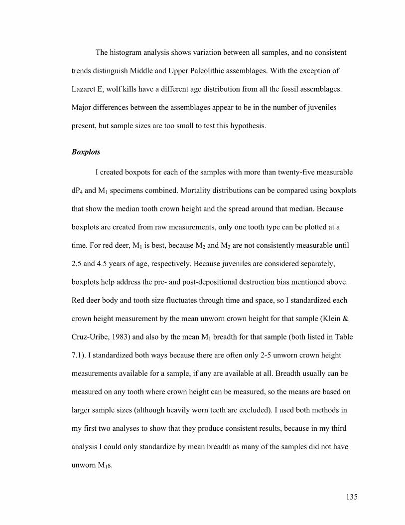
135

The histogram analysis shows variation between all samples, and no consistent

trends distinguish Middle and Upper Paleolithic assemblages. With the exception of

Lazaret E, wolf kills have a different age distribution from all the fossil assemblages.

Major differences between the assemblages appear to be in the number of juveniles

present, but sample sizes are too small to test this hypothesis.

Boxplots

I created boxpots for each of the samples with more than twenty-five measurable

dP4 and M1 specimens combined. Mortality distributions can be compared using boxplots

that show the median tooth crown height and the spread around that median. Because

boxplots are created from raw measurements, only one tooth type can be plotted at a

time. For red deer, M1 is best, because M2 and M3 are not consistently measurable until

2.5 and 4.5 years of age, respectively. Because juveniles are considered separately,

boxplots help address the pre- and post-depositional destruction bias mentioned above.

Red deer body and tooth size fluctuates through time and space, so I standardized each

crown height measurement by the mean unworn crown height for that sample (Klein &

Cruz-Uribe, 1983) and also by the mean M1 breadth for that sample (both listed in Table

7.1). I standardized both ways because there are often only 2-5 unworn crown height

measurements available for a sample, if any are available at all. Breadth usually can be

measured on any tooth where crown height can be measured, so the means are based on

larger sample sizes (although heavily worn teeth are excluded). I used both methods in

my first two analyses to show that they produce consistent results, because in my third

analysis I could only standardize by mean breadth as many of the samples did not have

unworn M1s.

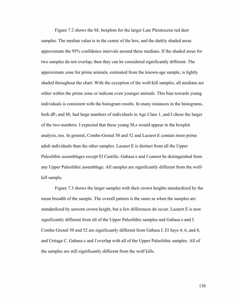
136

Figure 7.2 shows the M1 boxplots for the larger Late Pleistocene red deer

samples. The median value is in the center of the box, and the darkly shaded areas

approximate the 95% confidence intervals around these medians. If the shaded areas for

two samples do not overlap, then they can be considered significantly different. The

approximate zone for prime animals, estimated from the known-age sample, is lightly

shaded throughout the chart. With the exception of the wolf-kill samples, all medians are

either within the prime zone or indicate even younger animals. This bias towards young

individuals is consistent with the histogram results. In many instances in the histograms,

both dP4 and M1 had large numbers of individuals in Age Class 1, and I chose the larger

of the two numbers. I expected that these young M1s would appear in the boxplot

analysis, too. In general, Combe-Grenal 50 and 52 and Lazaret E contain more prime

adult individuals than the other samples. Lazaret E is distinct from all the Upper

Paleolithic assemblages except El Castillo. Gabasa e and f cannot be distinguished from

any Upper Paleolithic assemblage. All samples are significantly different from the wolf-

kill sample.

Figure 7.3 shows the larger samples with their crown heights standardized by the

mean breadth of the sample. The overall pattern is the same as when the samples are

standardized by unworn crown height, but a few differences do occur. Lazaret E is now

significantly different from all of the Upper Paleolithic samples and Gabasa e and f.

Combe-Grenal 50 and 52 are significantly different from Gabasa f, El Juyo 4, 6, and 8,

and Urtiaga C. Gabasa e and f overlap with all of the Upper Paleolithic samples. All of

the samples are still significantly different from the wolf kills.

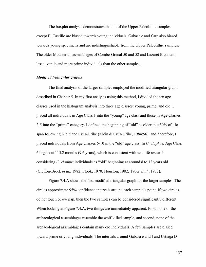
137

The boxplot analysis demonstrates that all of the Upper Paleolithic samples

except El Castillo are biased towards young individuals. Gabasa e and f are also biased

towards young specimens and are indistinguishable from the Upper Paleolithic samples.

The older Mousterian assemblages of Combe-Grenal 50 and 52 and Lazaret E contain

less juvenile and more prime individuals than the other samples.

Modified triangular graphs

The final analysis of the larger samples employed the modified triangular graph

described in Chapter 5. In my first analysis using this method, I divided the ten age

classes used in the histogram analysis into three age classes: young, prime, and old. I

placed all individuals in Age Class 1 into the “young” age class and those in Age Classes

2-5 into the “prime” category. I defined the beginning of “old” as older that 50% of life

span following Klein and Cruz-Uribe (Klein & Cruz-Uribe, 1984:56), and, therefore, I

placed individuals from Age Classes 6-10 in the “old” age class. In C. elaphus, Age Class

6 begins at 115.2 months (9.6 years), which is consistent with wildlife research

considering C. elaphus individuals as “old” beginning at around 8 to 12 years old

(Clutton-Brock et al., 1982; Flook, 1970; Houston, 1982; Taber et al., 1982).

Figure 7.4.A shows the first modified triangular graph for the larger samples. The

circles approximate 95% confidence intervals around each sample’s point. If two circles

do not touch or overlap, then the two samples can be considered significantly different.

When looking at Figure 7.4.A, two things are immediately apparent. First, none of the

archaeological assemblages resemble the wolf-killed sample, and second, none of the

archaeological assemblages contain many old individuals. A few samples are biased

toward prime or young individuals. The intervals around Gabasa e and f and Urtiaga D

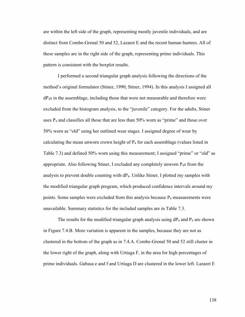
138

are within the left side of the graph, representing mostly juvenile individuals, and are

distinct from Combe-Grenal 50 and 52, Lazaret E and the recent human hunters. All of

these samples are in the right side of the graph, representing prime individuals. This

pattern is consistent with the boxplot results.

I performed a second triangular graph analysis following the directions of the

method’s original formulator (Stiner, 1990; Stiner, 1994). In this analysis I assigned all

dP4s in the assemblage, including those that were not measurable and therefore were

excluded from the histogram analysis, to the “juvenile” category. For the adults, Stiner

uses P4 and classifies all those that are less than 50% worn as “prime” and those over

50% worn as “old” using her outlined wear stages. I assigned degree of wear by

calculating the mean unworn crown height of P4 for each assemblage (values listed in

Table 7.3) and defined 50% worn using this measurement; I assigned “prime” or “old” as

appropriate. Also following Stiner, I excluded any completely unworn P4s from the

analysis to prevent double counting with dP4. Unlike Stiner, I plotted my samples with

the modified triangular graph program, which produced confidence intervals around my

points. Some samples were excluded from this analysis because P4 measurements were

unavailable. Summary statistics for the included samples are in Table 7.3.

The results for the modified triangular graph analysis using dP4 and P4 are shown

in Figure 7.4.B. More variation is apparent in the samples, because they are not as

clustered in the bottom of the graph as in 7.4.A. Combe-Grenal 50 and 52 still cluster in

the lower right of the graph, along with Urtiaga F, in the area for high percentages of

prime individuals. Gabasa e and f and Urtiaga D are clustered in the lower left. Lazaret E

139

has the highest percentage of old individuals, but this point is encompassed by a large

density contour that is significantly different only from Gabasa e and f and Urtiaga D.

Both modified triangular graph analyses show that there is considerable overlap

of age distributions in the Middle and Upper Paleolithic assemblages. Most samples do

not contain very many old individuals and primarily differ in the number of juveniles that

they contain.

Summary

In all of the analyses, some Middle Paleolithic samples cannot be distinguished

from Upper Paleolithic samples, suggesting that at least some Neandertals hunted in

similar ways to modern humans. Most of the variation between samples is in the number

of juvenile individuals, whether indicated by dP4 or slightly worn M1s. This variation

might be due to differences in hunting, transportation of mandibles of different ages back

to the cave sites, the degree of carnivore ravaging, or post-depositional histories. Urtiaga

F and particularly El Castillo have fewer juveniles than the other Magdalenian

assemblages. Multiple results show that Lazaret E has a greater abundance of older

individuals than the other samples, although this is not always statistically significant.

Lazaret E is the oldest assemblage included in these analyses, and its stone tool industry

is from around the time of the transition from Acheulean to Mousterian in southern

France. If later Middle Paleolithic people were hunting in ways indistinguishable from

Upper Paleolithic peoples, as indicated by Gabasa e and f, then Lazaret E could be

showing changes in hunting practices that might have co-occurred with changes in stone

tools. More samples and better understanding of the depositional history of these samples

will help test this idea.

140

Second analysis: Grouped samples

Sample definition

For my second analysis of the red deer fossil specimens, I wanted to include more

assemblages to see if they confirmed the patterns that I detected in my first analysis. For

this analysis I also wanted to increase my sample sizes, and the only way I could do this

was to group multiple samples together. Granted, lumping can obscure fine patterns seen

between stratigraphic layers, but my approach to this project was to attempt many

different ways of looking at the data and base my conclusions on patterns that repeatedly

emerge. I began by grouping layers within one site by their tool assemblages. By doing

this, a La Riera Solutrean sample was added; no Solutrean assemblages were included in

the first analysis. The Magdalenian layers from Urtiaga and El Juyo included in the first

analysis are each grouped into a sample. All of the layers from Gabasa and Lazaret are

now included; hopefully larger samples from these unique sites will help illuminate their

histories. I grouped all Combe-Grenal samples into layers 1-35 and 36-54. Although

these assemblages are defined as different Mousterian facies, I chose to group them in

this way because other aspects of the deposits show a break at this time (Delpech, 1996).

Grouping these layers allows much more of this rich site to be studied. Finally, I grouped

all of the Azilian samples from northern Spain so that this most recent time period could

be included; Urtiaga C is included in this sample. Summary statistics for the samples

considered in these analyses are listed in Table 7.4, and full descriptions are provided in

Appendix D. My methods for analyzing the age distributions are exactly the same as for

my first fossil analysis and are described in Chapter 5, so I will not repeat them here.

141

Histograms

Consistent with the first histogram analyses, the grouped samples differ primarily

in the number of juveniles relative to the subsequent age classes. El Castillo, El Juyo,

Gabasa, La Riera, and the wolf kills all have higher numbers of individuals in Age Class

1 than in the subsequent age classes. In contrast, Combe-Grenal 1-35 and 36-54, Lazaret,

and the recent hunters all have similar numbers of individuals in Age Class 1 and the

immediately subsequent ages classes. Combe-Grenal 1-35 is unique in that it is the only

sample where the number of individuals in each age class increases as the age classes get

older. Lazaret E in the first analysis is the only sample that is comparable, because this

sample has the same number of individuals in Age Classes 1, 2, and 3.

The Kolmogorov-Smirnov results show that none of the Upper Paleolithic

assemblages are significantly different from each other (Table 7.5.A). All of the Middle

Paleolithic assemblages are significantly different from the Upper Paleolithic

assemblages with the exceptions of Gabasa with the north Spanish Azilian sample and

Combe-Grenal 36-54 with La Riera. Gabasa is also significantly different from the other

three Mousterian samples, suggesting that this site is unique. The two Combe-Grenal

samples are significantly different from each other, but neither sample is significantly

different from Lazaret. All fossil samples are significantly different from the wolf-kill

sample and the model attritional structure, although most samples are also significantly

different from the recent human hunters and the model living age structure. Lazaret is not

significantly different from the model living age structure.

Grouping the samples created large enough sample sizes so that I was able to

compare only the adult distributions, excluding Age Class 1, using the Kolmogorov-

142

Smirnov test (Table 7.5.B). The northern Spanish Azilian and Gabasa samples were too

small to include in the analysis. The Upper Paleolithic samples are not significantly

different from each other, and many of the differences between the Upper and Middle

Paleolithic samples are no longer significant. Combe-Grenal 1-35 is still significantly

different from El Juyo and Urtiaga, and Lazaret is still significantly different from El

Juyo. Combe-Grenal 1-35 and 36-54 are no longer statistically different from either other

and are still not significantly different from Lazaret. All of the samples remain

significantly different from the wolf-kill sample and the model attritional profile. Many

of the significant differences between the fossil samples, the human hunters, and the

model living age structure are no longer present. These results confirm that many of the

differences between samples are due to the proportion of juveniles present relative to the

adults in the sample.

The proportion of juveniles present thus accounts for most of the variation

between samples and causes most of the distinctions between the Middle and Upper

Paleolithic. Most of the Middle Paleolithic samples have few juvenile individuals

compared to adults. The Gabasa sample is unique, because it has a very high proportion

of juveniles and is more similar to the Upper Paleolithic samples than are the other

Middle Paleolithic samples. When juveniles are eliminated, the most of the samples are

statistically indistinguishable. The question remains about whether or not the variation in

dP4s reflects hominid behavior or pre- or post-depositional destruction of deciduous teeth.

Boxplots

Figure 7.6 shows boxplots of the median M1 crown heights from the grouped

samples standardized by the mean unworn crown height calculated from that sample, and

143

Figure 7.7 shows the same samples but crown heights are standardized by the mean M1

breadth of the sample (Table 7.4 provides the values). Both analyses show similar results,

indicating that both adequately standardize the samples. In both analyses, Combe-Grenal

1-35 and 36-54 and Lazaret have median crown heights that are significantly lower than

Gabasa and all of the Upper Paleolithic samples except El Castillo. Gabasa resembles the

Upper Paleolithic samples, and this assemblage, northern Spanish Azilian, El Juyo, and

La Riera contain large numbers of young individuals. El Castillo contains the fewest of

the Upper Paleolithic sites.

Modified triangular graphs

In the last analysis, I plotted the grouped samples on the modified triangular

graphs using the age classes from the histogram analysis derived from dP4 and M1

(Figure 7.8.A) and using dP4 and P4 (Figure 7.8.B; samples summarized in Table 7.6), as

I described above. In the analysis of dP4 and M1, all of the samples are distinct from the

wolf-kill sample. Most of the variation is in the percentage of juveniles present, but

Combe-Grenal 1-35 and Lazaret do contain more old individuals. Combe-Grenal 1-35 is

distinct from all of the samples except for Lazaret. Lazaret and Combe-Grenal 36-54

overlap with each other and La Riera, Urtiaga, and the recent human hunters; these

samples plot on the right of the graph showing an abundance of prime individuals, and

they are distinct from all other Upper Paleolithic assemblages and Gabasa. Gabasa plots

in the far left of the graph and has the highest abundance of juveniles. It overlaps

primarily with El Castillo and to a much lesser extent with the northern Spanish Azilian.

The dP4 and P4 analysis shows more separation between the samples (Figure

7.8.B). El Castillo and the recent human hunters were excluded from the analysis because

144

measurements on P4 were unavailable. The 95% confidence interval of the wolf-kill

sample just barely overlaps with the 95% confidence interval of Lazaret. Lazaret has the

highest proportion of old individuals and overlaps only with Combe-Grenal 1-35.

Combe-Grenal 1-35 overlaps with El Juyo, too, but not Combe-Grenal 36-54. At the 95%

confidence level, the Upper Paleolithic samples are not significantly different from each

other, except for El Juyo and Urtiaga. The Gabasa sample is isolated in the far left of the

graph showing a high abundance of juveniles.

The modified triangular graph analyses show that Combe-Grenal 1-35 and

Lazaret have higher proportions of old individuals than the other samples and are for the

most part distinct from the Upper Paleolithic samples; Combe-Grenal 36-54 is more

similar to the Upper Paleolithic samples. Gabasa is distinct with its high percentage of

juveniles. The Upper Paleolithic samples vary among themselves mainly in the

percentages of juveniles compared to adults; all have low proportions of old individuals.

Summary

The results of the analyses using grouped samples are consistent with those for

the samples defined by stratigraphic layers. Lazaret and Combe-Grenal 1-35 are similar

to each other and distinct from the Upper Paleolithic assemblages. Combe-Grenal 36-54

is not as distinct, which is intriguing because it is the more ancient of the two Combe-

Grenal samples. Gabasa is unique among the Middle Paleolithic assemblages and is often

indistinguishable from the Upper Paleolithic samples, interesting because it is the

youngest of the Middle Paleolithic samples. The Azilian, Magdalenian, and Solutrean

samples are all similar, with the exception of El Castillo. This sample has a larger

145

percentage of dP4s, but a lower median M1 crown height. None of the archaeological

assemblages resemble the wolf-killed elk sample.

Third analysis: Many samples

Boxplots

Sample definition

In order to maximize the number of samples that could be included, my final

analysis incorporated all samples with ten or more measurable M1s. These samples were

grouped samples, sometimes encompassing many layers from a site or layers from

multiple closely grouped sites, as described for the second analysis. All of the samples

from the second analysis above are included. I added an additional sample composed of

multiple Epipaleolithic (= final Paleolithic) Federmesser assemblages from the Neuwied

Basin region of Germany and a Mesolithic sample from Star Carr, England. I also

included the Magdalenian layers from Altamira and La Riera and the Solutrean material

from Altamira. The Châtelperronian assemblage from Labeko Koba in northeastern

Spain, the early Mousterian assemblage from Piegu in northern France, and the Acheulo-

Yabrudian material from Tabun in Israel are all large enough to be included. Figure 3.2

provides a map of the sites, and Table 7.7 lists summary statistics, including the

percentage of dP4s in each sample. Appendix D provides more detailed information about

each assemblage. In this analysis, I standardized M1 crown height medians by mean

breadth only; sample sizes of unworn M1 crown heights were very small or absent, and

previous analyses showed that both standardization techniques provide consistent results.

146

Results

Figure 7.9 shows boxplots of these many samples in approximately chronological

order and grouped by tool industry. The most recent Paleolithic samples and the German

Federmesser and Azilian samples from northern Spain have an abundance of young

individuals. Of the Magdalenian assemblages, El Juyo and La Riera are comparable to

the more recent assemblages, while the other Magdalenian samples and the Mesolithic

Star Carr sample have medians that are solidly within the prime-age zone. The Solutrean

assemblages are indistinguishable from the Magdalenian and more recent samples. The

Châtelperronian assemblage from Labeko Koba is interesting not only because its median

is comparable to the Upper Paleolithic medians and Gabasa, but also because the crown

heights are tightly clustered. This is unusual in a sample of only 12 individuals. Among

the Mousterian samples, the median of the Gabasa sample shows a high abundance of

juvenile individuals and is indistinguishable from all of the Upper Paleolithic samples.

The median of the Combe-Grenal 1-35 sample is significantly lower than the Upper

Paleolithic samples’ medians, but Combe-Grenal 36-54 is not significantly different from

five of the nine Upper Paleolithic samples. Of the Early Mousterian assemblages, Lazaret

has more old specimens than each of the Upper Paleolithic samples, including Labeko

Koba, and Gabasa. However, the contemporaneous or slightly older sample of Piegu

from northern France overlaps with most of the Upper Paleolithic assemblages, except

the Azilian sample and El Juyo, and it is distinct from Labeko Koba and Gabasa. The

Tabun sample has more old individuals than the Azilian sample, El Juyo, the Solutrean

sample from Altamira, Labeko Koba, and Gabasa. All samples are significantly different

from the wolf-kill sample.

147

In sum, Mousterian and Acheulean samples overlap with some of the Upper

Paleolithic samples. The Gabasa sample, the youngest of the Middle Paleolithic samples,

is indistinguishable from the Upper Paleolithic assemblages in all analyses. Although

there is variation present, in general the older Mousterian assemblages are more biased

towards older red deer individuals than the Upper Paleolithic assemblages. The one

Châtelperronian sample included in this analysis follows the Upper Paleolithic pattern.

Bivariate plots

Sample definition

For my final set of analyses, I included all samples with ten or more measurable

first molars. I defined the samples as in my first analyses where each layer of each site

was considered separately. There were two exceptions: the grouped Federmesser sample

used in the second analysis and a grouped sample of the Acheulo-Yabrudian layers (E)

from Tabun in Israel. By considering smaller samples, I was able to include many

additional assemblages. Table 7.8 lists the samples and provides the summary

information, and Appendices C and D provide more details, including references. Table

7.8 also provides the relevant contextual information included in the following analyses.

Median crown height by date

Figure 7.10 plots the median M1 crown height for each sample standardized with

the mean M1 breadth for that sample by the sample’s approximate age in thousands of

years ago. The dates derive from multiple dating techniques, including radiometric dating

and biostratigraphy, and are shown without confidence intervals. They are mainly used to

place samples in relative sequence on the graph. Inspection of the graph produces striking

148

results. All samples from 60 kya or older all have median crown heights that indicate

higher numbers of older prey than samples from 50 kya younger. I tested the strength of

this relationship using Spearman’s rho (r = -0.74, p < 0.0001) and Kendall’s Tau (r = -

0.51, p = 0.0001), because neither data set is expected to be normally distributed. Both

tests showed a strong negative relationship between time and median crown height. The

data are clustered into two groups, which may be artificially inflating the strength of the

relationship, but the pattern is still clear.

The Mousterian tool industry spans the shift at 50 kya, and the most recent

Mousterian samples are similar to the Upper Paleolithic samples, including the

Châtelperronian, while the older Mousterian samples are similar to the even more ancient

assemblages. The two recent Mousterian assemblages that cluster with the Upper

Paleolithic are both from Gabasa Cave and have clustered with the Upper Paleolithic

assemblages in all the above analyses. All of the medians of the more ancient samples fall

below the grand mean of all the samples, although they are still the range for prime adult

red deer.

Median crown height by red deer abundance

I next wanted to investigate if there was a relationship between the proportion of

red deer hunted by prehistoric people and the ages of the animals hunted. Because red

deer abundance changes with environmental variables, the percentage of red deer can

provide an indicator of the local environmental conditions, if we assume that human

hunters were taking prey in equal abundance to their proportions on the landscape. Also,

by knowing the percentage of red deer in an assemblage, it may be possible to determine

if red deer were hunted differently depending on whether or not they were the primary

149

prey item or taken only occasionally. I measured the abundance of red deer as the

percentage of red deer by NISP in the total ungulate assemblage.

There is no visible patterning in the relationship between red deer abundance and

prey age at death; points plot in all corners of the graph (Figure 7.11.A). Spearman’s rho

(r = 0.01, p = 0.96) and Kendall’s Tau (r = 0.01, p = 0.94) also show that there are no

correlations in the data. Not surprisingly, many samples plot in the abundant end of the

graph, because these were the European assemblages that provided the largest sample

sizes. The patterning in the graph seems to be by industry, and samples representing all

tool industries plot in the abundant red deer portion of the graph. The early Mousterian

samples have the lowest medians (0.5-0.9) while the Magdalenian samples have the

highest (1.0-1.3). The percentage of red deer in Mousterian samples ranges from 23-87%;

samples with low percentages have both high (1.2 and 1.3) and low (0.6 and 0.7)

medians. Magdalenian samples with approximately the same median (1.0-1.1) plot in the

high, medium, and low abundance portions of the graph (40-95%).

Median crown height by temperature

As listed in Table 7.8, some assemblages have environmental conditions

associated with them. These are from the published descriptions of the site and are based

on various sources of data, including pollen, sedimentology, and large and small

mammals. The temperatures listed in site descriptions were rarely more specific than

cold, cool, or temperate. Figure 7.11.B plots the median M1 crown heights standardized

with mean M1 breath for the sample by temperature. Visually inspecting the graph, it is

possible to see that the sample distributions overlap. Because I would not expect the

samples to be normally distributed, I ran the Wilcoxon rank sum test (p = 0.65) and the

150

median test (p = 0.60), and neither showed a significant difference between the cold and

temperate samples. The distributions of the median crown heights actually did not deviate

from normal, so I also ran the student’s t-test (p = 0.51). This test is more likely to find

differences than the non-parametric tests. No significant difference can be detected in the

median ages of the red deer hunted during cold and temperate periods of both the Middle

and Upper Paleolithic.

Discussion

Variation in the number of juveniles

There is a large amount of variation in the percentages of juveniles, represented

by dP4s, in the samples, but this variation does not appear to be systematic. There is no

significant difference in the proportion of dP4s present between the assemblages

accumulated by Neandertals and those accumulated by modern humans (Table 7.8,

Wilcoxon test: p > 0.47, Median test: p > 0.14). Differences in the percentages of

juveniles may be due to differences in hunting practices or pre- and post-depositional

histories. Juvenile bones and deciduous teeth are not fully ossified and, therefore, are

more susceptible to carnivore ravaging, compaction, fragmentation, and soil leaching

than adult specimens, which will eliminate them from the fossil record (Hulbert, 1982;

Klein et al., 1983; Klein & Cruz-Uribe, 1984; Kurtén, 1953; Lyman, 1994; Munson,

2000).

It may be possible to control for biases caused by pre- and post-depositional

destruction to better estimate the composition of the original assemblage. One way is to

discount deciduous teeth and use boxplots to compare wear on only permanent teeth.

151

Lightly worn M1s do indicate the presence of younger individuals in an assemblage,

although the very youngest will not be included. Pre-depositional destruction can be

assessed by looking for evidence of carnivore damage, such as skeletal part

representation, gnaw marks, and gastric acid marks (Cruz-Uribe, 1991; Lyman, 1994;

Marean & Spencer, 1991). The degree of post-depositional loss can be considered by

examining the surface condition of the bones, the degree of fragmentation, and skeletal

part representation (Lyman, 1994). If skeletal part representation is highly correlated with

the density of those parts where the most abundant elements are the densest elements,

then juvenile specimens were likely lost (Lyman, 1984; Lyman, 1985). Samples with

similar kinds of biases should be compared only to each other or only using boxplots.

Only once differences in the representation of dP4s has been considered in light of pre-

and post-depositional destruction can investigators firmly conclude differences in the

hunting of juveniles. Because the goal of this study was to compare as many assemblages

as possible, I was unable to conduct detailed analyses of all the bone assemblages. In

many cases previous researchers had already conducted these analyses, but their data

were not always comparable. Therefore, for this study, boxplots are the best method for

investigating mortality profiles when destructive processes cannot be controlled for

adequately.

Hunting during the Upper Paleolithic

The Upper Paleolithic assemblages have an abundance of young adult animals.

The histogram analyses show a high number of individuals in Age Class 1, and the

median crown heights for these samples are very near the line distinguishing prime from

young individuals. By the time M1 erupts enough for the crown height to be measurable,

152

the animal is about 1.5 years old. Because boxplots only consider M1s and the M1s have

been measured, the individuals are likely to be at least 1.5 years old. However, in many

archaeological assemblages, teeth are commonly isolated from their mandibles, so M1s of

individuals younger than 1.5 years are often measured.

The Magdalenian sample from El Castillo is an exception to the trend of an

abundance of young animals in Upper Paleolithic assemblages. El Castillo and El Juyo 4

can be compared, because they are roughly contemporaneous and from the same

geographic region. They both contain about 47% juveniles, as indicated by the number of

dP4s, yet El Castillo’s median M1 crown height is significantly lower than the median M1

crown height of El Juyo in most of the analyses. It is possible that these two groups had

different hunting strategies for red deer. El Juyo is closer to the present coastline, while

El Castillo is further inland, and perhaps the Magdalenian people hunted red deer during

different seasons in the two locations. Cementum annuli studies of seasonality could

address this. It is also possible the red deer from El Juyo and El Castillo had different

diets, and therefore their teeth wore at different rates. In this case, the hunters from El

Juyo and El Castillo could have been hunting the same age prey, but the environment

around El Castillo made their teeth wear faster. A final possibility is that the two

assemblages experienced different amounts of post-depositional destruction. More of the

El Juyo M1 sample is composed of isolated teeth (28%) than the El Castillo sample (2%),

and so M1s from younger individuals may have been more readily measured in the El

Juyo sample.

My results agree with Pike-Tay’s (1991) study of mortality profiles in red deer

from Upper Paleolithic assemblages in southwestern France. Pike-Tay (1991) found that

153

the age distributions of prey from Magdalenian and Azilian assemblages had many more

juvenile than adult specimens in comparison to the model living age structure, while the

early Upper Paleolithic samples more closely resembled the model living age structure.

She hypothesized that the pattern was the result of the later people hunting with spear

throwers, while the early Upper Paleolithic people lacked projectile technology. My

Solutrean, Magdalenian, and Azilian samples also show an abundance of young adults.

These people could have been hunting with spear-throwers, so this is one explanation for

the patterning in the data. Unfortunately, none of my early Upper Paleolithic samples

contained enough individuals to include in the analyses.

An alternative explanation is that the Upper Paleolithic red deer were being

heavily exploited, possibly as a result of increasing human population densities. As

discussed in the introductory chapter, there is evidence that Upper Paleolithic people

were living at higher population densities and intensifying their use of the environment

by acquiring more fish and birds than their Middle Paleolithic predecessors. It is possible

that these larger human populations were exerting more pressure on red deer populations

than the animals experienced during most of the Middle Paleolithic, resulting in a

skewing of the living herd structure towards younger individuals. This type of

overexploitation pressure is visible in simulations of life tables (Taber et al. 1982). It also

is apparent in the histogram of the known-age elk that were killed by contemporary

hunters in Montana (Figure 5.2). Males over six years of age either are in low abundance

in the population (K. Hamlin, personal communication) or are inaccessible to hunters

given the terrain and regulations, so the modern-human-hunting mortality profile shows

154

an abundance of individuals in the younger adult age classes and fewer in the prime and

old classes compared to a typical herd.

Comparison of the Middle to the Upper Paleolithic

The Mousterian and more ancient assemblages have more prime individuals than

the Upper Paleolithic assemblages, including the Châtelperronian; the medians of the two

groups are mutually exclusive (Figure 7.10). But there is one exception, the assemblages

from Gabasa Cave, the most recent Mousterian site included in the study. These

Mousterian assemblages cluster with the Upper Paleolithic samples in having more

young specimens. This possible change in hunting during the Middle Paleolithic supports

Stiner’s (1990) conclusion that a shift in hunting strategies occurred approximately 45-55

kya. While my data support Stiner’s hypothesis, these conclusions are only tentative

because of the limited sampling involved. Gabasa is only one site with two larger

assemblages.

It is important to note that Stiner (1990) suggested that the more ancient

Neandertals were acquiring more prey by scavenging, while after 45-55 kya, they hunted

in ways that resemble modern humans. My data do not provide evidence of scavenging,

because the medians for all samples fall squarely within the prime zone or younger on the

boxplots. My data show a shift from hunting prime animals to young adults. The Upper

Paleolithic people and the inhabitants of Gabasa were hunting an abundance of either

juvenile or young adult animals. My results confirm previous research showing that

Neandertals were capable hunters of adult ungulates.

My results can be compared to Pike-Tay’s (1991) study of hunting during the

Upper Paleolithic. Her early Upper Paleolithic samples had “catastrophic” mortality

155

profiles, while her more recent samples contained more young individuals. The early

Upper Paleolithic assemblages can be compared to Neandertal accumulated samples,

because both groups lacked projectile technology. Both Pike-Tay’s (1991) early Upper

Paleolithic hunters and my Mousterian hunters were taking adult prey in similar

proportions to their abundance on the landscape. Pike-Tay (1991:108) hypothesized for

the early Upper Paleolithic that this would require organized, cooperative interception

and detention; traps, pits or snares; or stalking and ambushing prey. Similar hunting

strategies may be postulated for the Neandertals.

My more ancient samples indicated hunting, while Stiner’s more ancient samples

indicated scavenging. The difference is in the proportion of old prey represented in the

samples, which may be due to our different methods for estimating age-at-death and

constructing mortality profiles. Stiner (1990) investigated mortality profiles using dP4

and P4 to determine the percentages of juvenile, prime, and old in each sample. By

visually assessing wear, she assigns all dP4s as “juvenile,” all P4s with crown heights less

than 50% worn as “prime,” and all P4s with crown heights more than 50% worn as “old.”

In my analyses, I defined my age classes for dP4 and P4 the same as Stiner did, but I

measured P4 crown height to determine the percentage of wear. I also performed

additional analyses with dP4 and M1where I assigned the three ages classes based on the

ten age-class values of the histogram method. I classified all of Age Class 1 as “juvenile,”

specimens in Age Classes 2-5 (less than 115.2 months or 9.6 years) as “prime,” and those

in Age Classes 6-10 as “old.” Assigning age classes using P4s instead of M1s created

more separation along the “old” axis, and some samples have even more old individuals

than the wolf-kill sample (Figures 7.4 and 7.8). It appears that P4 and M1 assign different

156

ages to the same individuals. The known-age sample shows that P4 becomes more than

half worn between 10-12 years of age, while M1s are considered “old” at 9.6 years of age.

This suggests that the modified QCHM may be slightly underestimating the ages of the

animals, and this problem needs further research. Primarily, I conclude that Neandertals

were regularly hunting prime individuals from the boxplots analyses, where I calculated

the “prime” zone for the boxplots using the known-age sample. All of the medians for the

more ancient samples clearly fall into this area indicating prime hunting. The discrepancy

between these results needs to be further investigated.

All of the fossil mortality profiles are different from the attritional profile that

resulted from wolf hunting. These results fully support previous studies in concluding

that Neandertals were capable hunters and did not obtain the majority of their meat by

scavenging. The sample that most closely resembles the wolf kills in some analyses is

Lazaret E. This sample was deposited approximately 170 kya and is one of the earliest

Mousterian assemblages; researchers have debated if the tools should actually be

classified as Acheulean, the preceding industry (P. Valensi, personal communication). At

first this may suggest that the ability to hunt adult animals occurred with the change from

the Acheulean to Mousterian industry, but two even more ancient assemblages, Piegu and

Tabun, were included in the final analysis, and they have younger animals. Although they

are not significantly different from Lazaret, they are also not significantly different from

many Upper Paleolithic samples. This older time period deserves more research.

Finally, there is no relationship between prey age-at-death and environment. Tool

industry and time, which strongly covary, have the strongest relationship with the

mortality distributions. Unfortunately, only coarse environmental variables were

157

available for this study, and more detailed data are needed for further investigation into

this issue.

Summary and conclusions

In summary, the age-at-death data show a clear relationship with time where more

ancient samples contain more prime individuals while more recent samples have many

young adults. This change does not occur with the Middle to Upper Paleolithic transition,

as expected, but actually occurs within the Mousterian perhaps 50 kya, similar to

previous research by Stiner (1990) in west-central Italy. These results are preliminary,

however, because they are based on limited samples and the break is seen between two

assemblages, Gabasa and the upper layers of Combe-Grenal, neither of which is securely

dated. Once data from additional samples are collected, this hypothesis of a change in

hunting during the Middle Paleolithic can be further tested.

There are two possible explanations for this shift in the red deer mortality profiles.

First, there could have been a change in hunting strategy, which could have been the

result of changes in social or spatial organization or in still undetected changes in tool

technology. Second, increasing human population densities may have placed hunting

pressure on local red deer populations. In either case, my results indicate that both

modern humans and Neandertals were able to regularly take fit, adult animals and did not

have to rely on the youngest, oldest, and infirm members of the red deer herd, although

they hunted these individuals, too. These results confirm that the ability to regularly hunt

prime adult animals is a human characteristic that distinguishes us from other carnivores,

but they also show that Neandertals were clearly very similar to us in that they also could

regularly hunt prime-aged prey.

158

Chapter 8: Summary and conclusions

Significance of this research

Fossil hominid morphology, archaeology, and genetics all indicate that the

Neandertals were replaced by modern humans in Europe 30-40 kya. The early modern

humans’ stone tool industries were more refined than the Neandertals’ Mousterian

industry, and they also contained bone, antler, and ivory fashioned into tools. The aim of

this research was to investigate if the changes in tool industries correlated with a

difference in the ability to hunt large ungulates. A difference in resource extraction ability

is one potential explanation for why modern humans were able to replace Neandertals,

because it could have enabled modern humans to have larger population sizes or

densities. I investigated this problem by focusing on the hunting of only one species, red

deer, so that I could better control for prey behavior. I used prey age-at-death as my

indicator of hunting strategies, because humans are unique in their ability to regularly

hunt prime adult individuals. In contrast, non-human carnivores usually take the young,

old, and infirm from a population.

My results show that Neandertals and modern humans did not differ significantly

in their ability to hunt prime-aged ungulates, and they both did so regularly. None of the

mortality distributions of the assemblages studied here resemble the distribution

constructed from wolf kills, suggesting that by at least 200 kya, hominids were hunting

differently than a top carnivore. There is a trend in the Paleolithic data for more recent

assemblages, those younger than 50 kya, to have more young adult animals, while the

159

more ancient sites, those older than 50 kya, have more prime red deer. This change

happened during the Middle Paleolithic and not with the change from Middle to Upper

Paleolithic as I would have expected. Stiner’s (1990) study of assemblages spanning the

Middle to Upper Paleolithic transition in west-central Italy also showed a shift in large

game use within the Middle Paleolithic about 40-50 kya, but she attributed this to a shift

from more scavenging to more hunting. These results should be taken cautiously and a

shift in hunting during the Middle Paleolithic should be considered a hypothesis for

future research, because only limited samples are available. In my samples, the

assemblages from only one Middle Paleolithic site show a mortality distribution that is

indistinguishable from the Upper Paleolithic samples, so this pattern needs to be

confirmed with more data.

The technological difference that most clearly distinguishes modern humans from

Neandertals is the working of bone, antler, and ivory into the formal tools and art objects

found in Upper Paleolithic industries. These new tools may have allowed modern humans

to more fully exploit new niches, including birds and aquatic resources. In addition, bone

and ivory needles and awls that are part of this new industry provide the earliest evidence

for tailored clothing, which may have played a role in allowing modern humans to live at

latitudes far north from where Neandertals have ever been found (Hoffecker, 1999).

This study also investigated the methods used to estimate the age-at-death of

fossil specimens and to construct mortality profiles from fossil assemblages. I conclude

that boxplots showing median tooth crown heights are the best method for assessing age

distributions. Boxplots are based on raw crown height measurements, so no detailed

knowledge about the relationship between tooth crown height and age are needed. Only

160

two assumptions are necessary, and they are true of all wear-based age determination

techniques. First, a more worn tooth indicates an older individual than a less worn tooth.

Second, tooth wear rates are comparable between populations. Unfortunately, boxplots

prevent detailed analyses of nuances in the age distribution such as is available with

histograms, but enough differences in age structure can be identified for meaningful

comparisons and interpretations. The boxplot method is more difficult to apply to species

whose average tooth size changes through time and space, such as C. elaphus, but

unworn crown height and average tooth breadth both appear to be adequate for

standardization. Ideally, histograms would be used to investigate mortality distributions,

but their widespread applicability is inhibited by the errors involved in translating tooth

crown heights into chronological ages and idiosyncratic differences due to small sample

sizes. I am confident that once more known-age samples are studied, the problem of

estimating chronological age can be addressed, but small sample size will always be an

issue when studying fossil assemblages.

Finally, I investigated the relationship between C. elaphus body size and climate.

Modern North American elk size correlates with climatic parameters to support

Bergmann’s rule. This relationship is stronger in sex divided analyses of distal

metacarpal breadths than it is in analyses of grouped male and female M1 breadths. This

is likely because skeletal elements are more plastic than teeth and more closely reflect

body mass and, therefore, will respond more readily to environmental changes. Western

European red deer metatarsals and teeth do not exhibit relationships with the climatic

parameters that would suggest that red deer follow Bergmann’s rule. Analyses are

confined by the fact that many of C. elaphus subspecies are extinct, which limits the

161

range of variation available for study. This is particularly evident in North America

where the southern-most and eastern-most subspecies no longer exist. The problem is

further complicated in both North America and western Europe by recent re-introductions

of individuals from different subspecies into areas where local populations have gone

extinct. Because skeletal size is so plastic and has been anecdotally noted to change

within one generation of introduction into a new area, these recent re-introductions may

not significantly affect patterning in distal metapodial breadth. The teeth are more

conservative, so they will maintain the size of the parent population for a longer period of

time, obscuring any relationship that tooth breadth may have once had with climate.

The Late Pleistocene red deer generally appear to follow Bergmann’s rule. They

are mostly larger during glacial cycles and smaller during the interglacial cycles. Until

the relationship between body size and climate is understood using data on modern

specimens, C. elaphus body size should not be used as a paleoclimatic indicator. Within a

well-documented region, however, red deer body size is useful as a biostratigraphic

indicator to place assemblages within a relative sequence or as supporting evidence for

other paleoenvironmental indicators.

Future research directions

The results of this study provide many indications of where future research should

be focused, and it is clear that there is still much to be done to understand how and why

modern humans replaced the Neandertals and ultimately the origins of fully modern

humans.

First, red deer mortality profiles from archaeological assemblages from all time

periods need to be more comprehensively studied. To further test some of the trends

162

found in this study, sampling needs focus on the late Middle Paleolithic and the

Aurignacian. Early Upper Paleolithic assemblages need to be studied in detail whenever

they are available. Epipaleolithic assemblages could be used to form an archaeological

baseline of modern human subsistence strategies for comparisons with the more ancient

assemblages. Studying more recent sites, as well as paleontological sites, will further our

understanding of how pre- and post-depositional biases impact mortality profiles.

Sampling should focus on areas where red deer were always abundant, such as Spain and

Italy, so large samples can be obtained for all time periods. This will allow many

variables to be controlled, and thus allow hunting strategies to be better investigated.

Second, the earliest Upper Paleolithic deserves more attention. In order to

understand fully how and why modern humans replaced the Neandertals, studies need to

directly compare the latest Mousterian with the earliest Upper Paleolithic. One criticism

of the archaeological evidence for the Out of Africa model is that “modern” characters do

not actually appear until later in the Upper Paleolithic, particularly with the Solutrean and

Magdalenian (Lindly & Clark, 1990; Straus, 1977; Straus, 1992). This bias towards

discussing later periods is because later Upper Paleolithic sites are more numerous in

western Europe, as evidenced by a population explosion during the Magdalenian

following the last glacial maximum (Bocquet-Appel & Demars, 2000b). However, early

Upper Paleolithic sites in Eastern Europe do show characteristics of “modern” behavior

very early. Much more detailed information on the early Aurignacian and its conspecifics

is needed, not only in western Europe, but also in eastern Europe and western Asia. As

the early Aurignacian becomes better known, it will be easier to make meaningful

163

comparisons with the late Mousterian. In addition, more data are needed on the Upper

Paleolithic assemblages created by Neandertals, such as the Châtelperronian.

Third, studies similar to the current one need to be conducted on other prey

species; reindeer, bison, aurochs, horse, and ibex would all be good subject species. The

best way to choose the next species for detailed comparisons is to determine which

species is most common is the earliest Upper Paleolithic assemblages. Because the

Mousterian extends back further in time, it may be easier to find suitable samples for

comparison in this more ancient period. Species of small animals should certainly be

included in future comparisons of Middle and Upper Paleolithic resource gathering

strategies. Current evidence indicates that the frequent exploitation of small game,

particularly fish and birds, is characteristic of the Upper Paleolithic. This is particularly

important because the exploitation of these species probably indicates more sophisticated

tool technology involving bone and ivory working. Comparisons of tortoise and shellfish

gathering across the Middle to Upper Paleolithic transition can also provide data on

population densities and resource intensification. Studying these small animals will

require the re-evaluation of many previously excavated assemblages and careful

excavation of new assemblages. Fortunately, saving the remains of these small animals is

now standard practice, and so much more data on small game exploitation should become

available in the near future.

Fourth, more detailed climatic data than were available for this study are needed.

Fortunately, many researchers are currently directly addressing this knowledge gap and

data sets are accumulating which will help with future research (Davies et al., 2000).

These data will help illuminate hunting strategies and also will be beneficial for knowing

164

what areas where inhabitable at certain times, which then could be linked to the migration

of modern humans into Europe. Around the time of the Middle to Upper Paleolithic

transition in Europe, climate was rapidly fluctuating (van Andel, 1998; van Andel &

Tzedakis, 1996). More research is needed on these paleoclimates before it is possible to

know what role these periods of change and stability played in modern human origins and

the replacement of the Neandertals.

Finally, all of these studies should be extended back in time to comparisons of the

early to the late Middle Paleolithic. The idea of a shift in behavior during this time is

intriguing. Knowing how Neandertals, our closest relatives, responded to changing

resources, climate, and possibly population pressure will help us better understand our

own adaptations. As for determining when people acquired the ability to regularly hunt

large game animals, more research is needed on more ancient times. I think that

comparisons between the Acheulean and the Middle Paleolithic will help illuminate this

issue.

Conclusions

This research shows that Neandertals were capable of regularly hunting prime-

aged red deer. The ability to regularly hunt prime-aged large prey distinguishes modern

humans from all other carnivores, and the data presented here demonstrate that hominids

had entered this niche by the time of the Neandertals at least 200 kya. However, the

samples included in this study show a shift in prey age-at-death during the Middle

Paleolithic approximately 50 kya. Young adult prey are more abundant in recent

assemblages than in more ancient assemblages. Over 25 archaeological samples from

throughout western Europe contributed to this conclusion, making this the most

165

comprehensive study to date. Because Neandertals and modern humans were both

capable of hunting the most desirable prey and could do so regularly, researchers must

explore other reasons than differences in big game hunting to explain the demise of the

Neandertals.

166

Appendix A Tables

Tab

le 3

.1 In

tero

bse

rver

mea

sure

men

t er

ror

for

too

th c

row

n h

eig

ht

and

bre

adth

Com

paris

on o

f mea

sure

men

ts ta

ken

on th

e sa

me

spec

imen

s by

the

auth

or a

nd o

ther

res

earc

hers

. R.G

. Kle

in a

nd th

e au

thor

mea

sure

d th

eB

ritis

h N

atur

al H

isto

ry M

useu

m's

C. e

laph

us c

ompa

rativ

e co

llect

ion,

and

C. W

olf a

nd th

e au

thor

mea

sure

d th

e kn

own-

age

elk

sam

ple.

The

sam

ples

are

poo

led

sam

ples

of d

P4,

P4,

M1,

M2

and

M3.

All

valu

es a

re in

mill

imet

ers.

mea

sure

men

tn

mea

nst

anda

rd d

evia

tion

min

imum

max

imum

crow

n he

ight

110

0.24

(2.

9%)

0.35

(4.

4%)

02.

8br

eadt

h81

0.29

(2.

5%)

0.29

(3.

1%)

0.01

1.4

Tab

le 3

.2. E

rup

tio

n a

nd

wea

r st

ages

rec

ord

ed in

th

is s

tud

yE

1 th

roug

h E

4 de

scrib

e st

ages

of t

ooth

eru

ptio

n, a

nd th

e ot

hers

des

crib

e w

ear.

Eru

ptin

g te

eth

wer

e no

t inc

lude

d in

any

of t

he a

naly

ses

disc

usse

d he

re. I

n co

mpl

ete

man

dibl

es, t

eeth

com

e in

to o

cclu

sion

bef

ore

the

crow

n-ro

ot ju

nctio

n is

vis

ible

, so

thei

r fu

ll cr

own

heig

hts

rem

ain

unm

easu

rabl

e at

you

ng a

ges.

Unw

orn

crow

n he

ight

s ca

n on

ly b

e re

cord

ed in

C. e

laph

us o

n is

olat

ed te

eth,

by

taki

ng X

-ray

s of

the

man

dibl

e, o

rby

cut

ting

the

bone

aw

ay fr

om th

e cr

own-

root

junc

tion

of th

e to

oth.

wea

r st

age

code

desc

riptio

n of

wea

r st

age

E1

toot

h st

ill in

cry

ptE

2to

oth

unw

orn

and

less

than

hal

fway

to o

cclu

sion

E3

toot

h un

wor

n an

d ov

er h

alfw

ay to

occ

lusi

onE

4to

oth

in o

cclu

sion

, but

cro

wn-

root

junc

tion

is n

ot v

isib

le, t

here

fore

cro

wn

heig

ht is

not

mea

sura

ble

UW

unw

orn

toot

h (n

ot y

et in

occ

lusi

on).

The

cro

wn-

root

junc

tion

is v

isib

le a

nd fu

ll cr

own

heig

ht is

mea

sura

ble

VE

Wve

ry e

arly

wea

r. T

here

is s

ome

wea

r on

the

ante

rior

or p

oste

rior

edge

of t

he c

usp,

but

the

crow

n he

ight

can

stil

l be

used

as a

n un

wor

n cr

own

heig

htLW

light

wea

r. C

usps

are

stil

l hig

h pe

aks

and

dent

ine

band

s ar

e na

rrow

MW

med

ium

wea

r. O

cclu

sal s

urfa

ce o

f the

cus

ps a

re r

ound

ed to

com

plet

ely

flat.

The

cro

wn

is a

ppro

xim

atel

y 30

-50%

wor

n.D

entin

e ba

nds

are

wid

eH

Whe

avy

wea

r. O

cclu

sal s

urfa

ce is

flat

and

the

crow

n is

mor

e th

an 5

0% w

orn.

Som

e in

fund

ibul

um r

emai

nsV

HW

very

hea

vy w

ear.

Infu

ndib

ulum

s ar

e ab

sent

. Ena

mel

of t

he c

row

n ne

arly

or

com

plet

ely

wor

n aw

ay

Tab

le 4

.1 S

um

mar

y o

f el

k sp

ecim

ens

wit

h k

no

wn

ag

esT

he n

umbe

r of

kno

wn-

age

elk

spec

imen

s in

the

orig

inal

Kle

in e

t al.

stud

ies

(198

1, 1

983a

, 198

3b; d

ata

colle

cted

by

C. W

olf)

plu

s th

e nu

mbe

r of

new

spe

cim

ens

adde

d in

this

stu

dy p

rovi

des

the

tota

l ind

ivid

uals

in th

e kn

own-

age

sam

ple.

The

num

ber

of c

row

n he

ight

s th

at w

ere

mea

sure

din

eac

h ag

e co

hort

is p

rovi

ded.

age

coho

rts

year

s (m

onth

s)or

igin

alne

wto

tal

mal

esfe

mal

esdP

4P

4M

1M

2M

3

0.5

(5-1

0)41

142

2715

421.

5 (1

7-20

)39

241

1920

4121

22.

5 (2

7-33

)25

1136

1515

33

361

3.5

(40-

44)

249

337

2322

335

4.5

(53-

57)

1411

256

1711

2510

25.

5 (6

5-68

)10

515

49

1515

134

6.5

(77-

79)

66

56

63

37.

5 (8

9-92

)1

78

78

87

48.

5 (1

01-1

04)

91

108

910

109

9.5

(113

-114

)3

33

33

33

10.5

11.5

(13

8)1

11

11

11

12.5

(15

0-15

6)2

22

22

22

13.5

14.5

(17

3)1

11

11

11

15.5

(18

5)2

21

12

22

216

.517

.518

.519

.520

.521

.5 (

260)

*1

11

11

1

tota

l17

056

226

7912

886

8416

361

32

* E

xclu

ded

from

all

anal

yses

Tab

le 4

.2 S

um

mar

y o

f re

gre

ssio

ns

of

age

on

cro

wn

hei

gh

t in

th

e kn

ow

n-a

ge

elk

sam

ple

The

sam

ple

size

s, m

ean

age

and

crow

n he

ight

, sta

ndar

d de

viat

ions

of a

ge a

nd c

row

n he

ight

, coe

ffici

ents

of d

eter

min

atio

n, a

nd s

tand

ard

erro

rsof

est

imat

e as

soci

ated

with

the

linea

r an

d qu

adra

tic r

egre

ssio

ns o

f age

on

crow

n he

ight

for

the

know

n-ag

e sa

mpl

e of

elk

.

sam

ple

info

rmat

ion

dP4

P4

M1

M2

M3

sam

ple

size

(n)

8683

163

6031

mea

n ag

e (m

onth

s)13

.472

.553

.581

.410

3.6

stan

dard

dev

iatio

n of

age

(m

onth

s)6.

434

.733

.136

.835

.5m

ean

crow

n he

ight

(m

m)

8.2

17.0

12.9

15.5

15.2

3st

anda

rd d

evia

tion

of c

row

n he

ight

(m

m)

2.6

3.8

4.3

5.0

4.6

linea

r re

gres

sion

coef

ficie

nt o

f det

erm

inat

ion

(r2 )

0.83

0.85

0.84

0.87

0.84

stan

dard

err

or o

f est

imat

e (m

onth

s)2.

6213

.28

13.2

613

.21

13.8

1qu

adra

tic r

egre

ssio

nco

effic

ient

of d

eter

min

atio

n (r

2 )0.

830.

870.

870.

900.

85st

anda

rd e

rror

of e

stim

ate

(mon

ths)

2.61

12.4

412

.09

11.3

513

.69

Tab

le 4

.3 S

um

mar

y o

f re

gre

ssio

ns

of

age

on

cro

wn

hei

gh

t th

e kn

ow

n-a

ge

wh

ite-

taile

d d

eer

sam

ple

The

sam

ple

size

s, m

ean

age

and

crow

n he

ight

, sta

ndar

d de

viat

ions

of a

ge a

nd c

row

n he

ight

, coe

ffici

ents

of d

eter

min

atio

n, a

nd s

tand

ard

erro

rsof

est

imat

e as

soci

ated

with

the

linea

r an

d qu

adra

tic r

egre

ssio

ns o

f age

on

crow

n he

ight

for

the

know

n-ag

e sa

mpl

e of

whi

te-t

aile

d de

er.

sam

ple

info

rmat

ion

dP4

M1

M2

M3

sam

ple

size

(n)

5510

991

42m

ean

age

(mon

ths)

11.5

22.1

24.7

630

.4st

anda

rd d

evia

tion

of a

ge (

mon

ths)

6.0

16.4

16.6

21.2

mea

n cr

own

heig

ht (

mm

)4.

48.

510

.611

.0st

anda

rd d

evia

tion

of c

row

n he

ight

(m

m)

1.4

1.6

1.6

2.1

linea

r re

gres

sion

coef

ficie

nt o

f det

erm

inat

ion

(r2 )

0.79

0.60

0.70

0.84

stan

dard

err

or o

f est

imat

e (m

onth

s)2.

6910

.33

9.01

8.30

quad

ratic

reg

ress

ion

coef

ficie

nt o

f det

erm

inat

ion

(r2 )

0.80

0.72

0.82

0.88

stan

dard

err

or o

f est

imat

e (m

onth

s)2.

678.

596.

937.

13

Tab

le 4

.4 V

alu

es u

sed

in t

he

Qu

adra

tic

Cro

wn

Hei

gh

t M

eth

od

The

she

ddin

g an

d er

uptio

n ag

es a

nd th

e un

wor

n cr

own

heig

hts

used

in th

e Q

CH

M fo

r es

timat

ing

age-

at-d

eath

in R

ocky

Mou

ntai

n el

k fr

omw

este

rn M

onta

na. A

ges

of e

rupt

ion

and

shed

ding

for

each

toot

h ar

e co

nsis

tent

acr

oss

popu

latio

ns o

f C. e

laph

us, b

ut u

nwor

n cr

own

heig

hts

need

to b

e de

term

ined

for

each

sam

ple.

Val

ues

are

from

Kle

in e

t al.

(198

3:53

) an

d K

lein

and

Cru

z-U

ribe

(198

4:49

-50)

and

are

bas

ed o

nQ

uim

by a

nd G

aab

(195

7) a

nd L

owe

(196

7). S

ee a

lso

Bro

wn

and

Cha

pman

(19

91:5

25).

AG

Epe

l (po

tent

ial e

colo

gica

l lon

gevi

ty)

= 1

92 m

onth

s (1

6 ye

ars)

age

(mon

ths)

estim

ated

unw

orn

toot

h ty

pesh

eder

upts

crow

n he

ight

(m

m)

dP4

2614

.0P

426

23.0

*M

16

27.0

M2

1229

.6M

330

31.0

* F

rom

this

stu

dy

Tab

le 4

.5 C

om

par

iso

n o

f re

gre

ssio

n a

nd

th

eore

tica

l eq

uat

ion

sR

egre

ssio

n eq

uatio

ns a

re b

ased

on

the

sam

ple

of k

now

n-ag

e el

k, a

nd th

e th

eore

tical

equ

atio

ns w

ere

calc

ulat

ed fo

r R

ocky

Mou

ntai

n e

lk u

sing

the

QC

HM

. Val

ues

used

to d

eriv

e th

e th

eore

tical

form

ulas

are

list

ed in

Tab

le 4

.4.

Reg

ress

ion

equa

tions

The

oret

ical

equ

atio

nsdP

4dP

4

Age

= 3

1.77

- 2

.241

CH

Age

= 2

6 -

1.85

7 C

HA

ge =

33.

925

- 2.

826

CH

+ 0

.036

CH

2A

ge =

26

- 3.

714

CH

+ 0

.133

CH

2

P4

P4

Age

= 2

14.3

01 -

8.3

60 C

HA

ge =

192

- 7

.217

CH

Age

= 2

69.0

18 -

16.

028

CH

+ 0

.249

CH

2A

ge =

192

- 1

4.43

5 C

H +

0.3

14 C

H2

M1

M1

Age

= 1

43.6

02 -

6.9

75 C

HA

ge =

192

- 6

.889

CH

Age

= 1

63.6

01 -

11.

522

CH

+ 0

.209

CH

2A

ge =

192

- 1

3.77

8 C

H +

0.2

55 C

H2

M2

M2

Age

= 1

86.8

19 -

6.8

10 C

HA

ge =

192

- 6

.081

CH

Age

= 2

18.5

3 -

11.5

95 C

H +

0.1

60 C

H2

Age

= 1

92 -

12.

162

CH

+ 0

.205

CH

2

M3

M3

Age

= 2

11.2

86 -

7.0

69 C

HA

ge =

192

- 5

.226

CH

Age

= 2

24.1

82 -

9.1

59 C

H +

0.0

75 C

H2

Age

= 1

92 -

10.

452

CH

+ 0

.169

CH

2

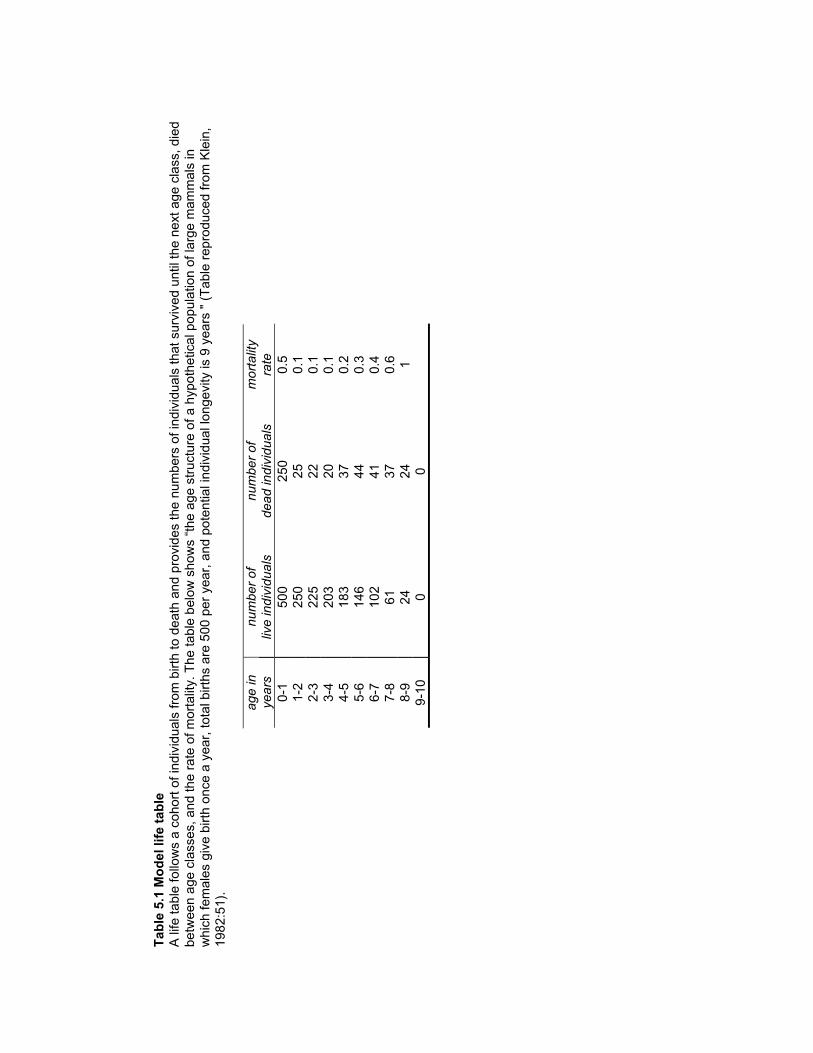
Tab

le 5

.1 M

od

el li

fe t

able

A li

fe ta

ble

follo

ws

a co

hort

of i

ndiv

idua

ls fr

om b

irth

to d

eath

and

pro

vide

s th

e nu

mbe

rs o

f ind

ivid

uals

that

sur

vive

d un

til th

e ne

xt a

ge c

lass

, die

dbe

twee

n ag

e cl

asse

s, a

nd th

e ra

te o

f mor

talit

y. T

he ta

ble

belo

w s

how

s “t

he a

ge s

truc

ture

of a

hyp

othe

tical

pop

ulat

ion

of la

rge

mam

mal

s in

whi

ch fe

mal

es g

ive

birt

h on

ce a

yea

r, to

tal b

irths

are

500

per

yea

r, a

nd p

oten

tial i

ndiv

idua

l lon

gevi

ty is

9 y

ears

" (

Tab

le r

epro

duce

d fr

om K

lein

,19

82:5

1).

age

innu

mbe

r of

num

ber

ofm

orta

lity

year

sliv

e in

divi

dual

sde

ad in

divi

dual

sra

te0-

150

025

00.

51-

225

025

0.1

2-3

225

220.

13-

420

320

0.1

4-5

183

370.

25-

614

644

0.3

6-7

102

410.

47-

861

370.

68-

924

241

9-10

00

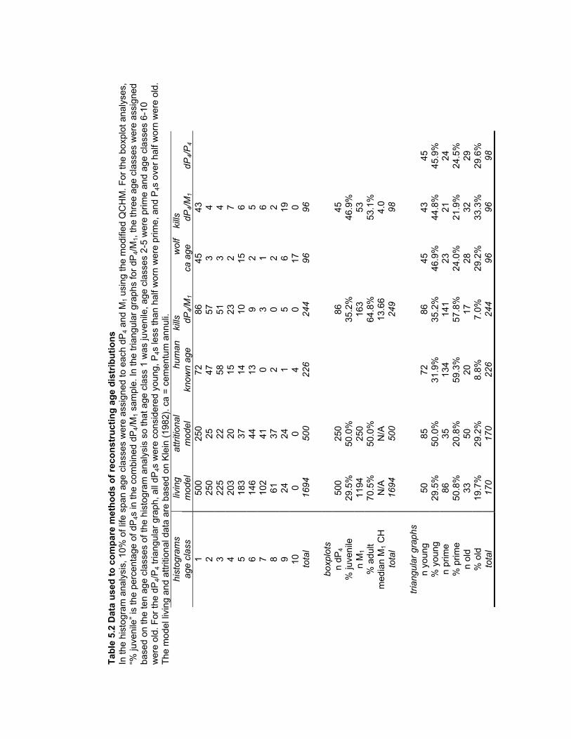
Tab

le 5

.2 D

ata

use

d t

o c

om

par

e m

eth

od

s o

f re

con

stru

ctin

g a

ge

dis

trib

uti

on

sIn

the

hist

ogra

m a

naly

sis,

10%

of l

ife s

pan

age

clas

ses

wer

e as

sign

ed to

eac

h dP

4 an

d M

1 us

ing

the

mod

ified

QC

HM

. For

the

boxp

lot a

naly

ses,

“% ju

veni

le”

is th

e pe

rcen

tage

of d

P4s

in th

e co

mbi

ned

dP4/

M1

sam

ple.

In th

e tr

iang

ular

gra

phs

for

dP4/

M1,

the

thre

e ag

e cl

asse

s w

ere

assi

gned

base

d on

the

ten

age

clas

ses

of th

e hi

stog

ram

ana

lysi

s so

that

age

cla

ss 1

was

juve

nile

, age

cla

sses

2-5

wer

e pr

ime

and

age

clas

ses

6-10

wer

e ol

d. F

or th

e dP

4/P

4 tr

iang

ular

gra

ph, a

ll dP

4s w

ere

cons

ider

ed y

oung

, P4s

less

than

hal

f wor

n w

ere

prim

e, a

nd P

4s o

ver

half

wor

n w

ere

old.

The

mod

el li

ving

and

attr

ition

al d

ata

are

base

d on

Kle

in (

1982

). c

a =

cem

entu

m a

nnul

i.hi

stog

ram

sliv

ing

attr

ition

alhu

man

kills

wol

fki

llsag

e cl

ass

mod

elm

odel

know

n ag

edP

4/M

1ca

age

dP4/

M1

dP4/

P4

150

025

072

8645

432

250

2547

573

43

225

2258

513

44

203

2015

232

75

183

3714

1015

66

146

4413

92

57

102

410

31

68

6137

20

22

924

241

56

1910

00

40

170

tota

l16

9450

022

624

496

96

boxp

lots

n dP

450

025

086

45%

juve

nile

29.5

%50

.0%

35.2

%46

.9%

n M

111

9425

016

353

% a

dult

70.5

%50

.0%

64.8

%53

.1%

med

ian

M1

CH

N/A

N/A

13.6

64.

0to

tal

1694

500

249

98

tria

ngul

ar g

raph

sn

youn

g50

8572

8645

4345

% y

oung

29.5

%50

.0%

31.9

%35

.2%

46.9

%44

.8%

45.9

%n

prim

e86

3513

414

123

2124

% p

rime

50.8

%20

.8%

59.3

%57

.8%

24.0

%21

.9%

24.5

%n

old

3350

2017

2832

29%

old

19.7

%29

.2%

8.8%

7.0%

29.2

%33

.3%

29.6

%to

tal

170

170

226

244

9696

98

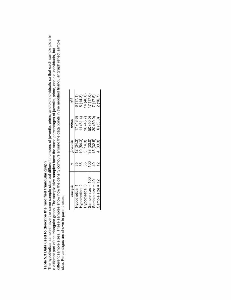
Tab

le 5

.3 D

ata

use

d t

o d

escr

ibe

the

mo

dif

ied

tri

ang

ula

r g

rap

hT

he h

ypot

hetic

al s

ampl

es h

ave

the

sam

e sa

mpl

e si

ze, b

ut d

iffer

ent n

umbe

rs o

f juv

enile

, prim

e, a

nd o

ld in

divi

dual

s so

that

eac

h sa

mpl

e pl

ots

ina

diffe

rent

par

t of t

he tr

iang

ular

gra

ph. T

he s

ampl

e si

ze s

ampl

es h

ave

the

sam

e pe

rcen

tage

s of

juve

nile

, prim

e, a

nd o

ld in

divi

dual

s, b

utdi

ffere

nt s

ampl

e si

zes.

The

se s

ampl

es s

how

how

the

dens

ity c

onto

urs

arou

nd th

e da

ta p

oint

s in

the

mod

ified

tria

ngul

ar g

raph

ref

lect

sam

ple

size

. Per

cent

ages

are

sho

wn

in p

aren

thes

es. sa

mpl

en

juve

nile

prim

eol

dH

ypot

hetic

al 1

3512

(34

.3)

17 (

48.6

)6

(17.

1)H

ypot

hetic

al 2

3519

(54

.3)

11 (

31.4

)5

(14.

3)H

ypot

hetic

al 3

355

(14.

3)16

(45

.7)

14 (

40.0

)S

ampl

e si

ze =

100

100

33 (

33.0

)50

(50

.0)

17 (

17.0

)S

ampl

e si

ze =

40

4013

(32

.5)

20 (

50.0

)7

(17.

5)S

ampl

e si

ze =

12

124

(33.

3)6

(50.

0)2

(16.

7)

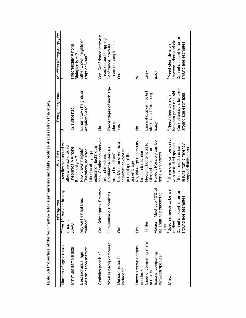
Tab

le 5

.4 P

rop

erti

es o

f th

e fo

ur

met

ho

ds

for

sum

mar

izin

g m

ort

alit

y p

rofi

les

dis

cuss

ed in

th

is s

tud

y

His

togr

ams

Box

plot

sT

riang

ular

gra

phs

Mod

ified

tria

ngul

ar g

raph

sN

umbe

r of

age

cla

sses

Ofte

n 10

, but

can

be

any

amou

ntJu

veni

les

sepa

rate

d ou

t,ot

herw

ise

not d

ivid

ed3

3

Min

imum

sam

ple

size

30-4

0T

heor

etic

ally

= n

one

Bio

logi

cally

= ?

12 s

ugge

sted

The

oret

ical

ly =

non

eB

iolo

gica

lly =

?B

est i

ndiv

idua

l age

dete

rmin

atio

n m

etho

dA

ny w

ell e

stab

lishe

dm

etho

da

Raw

cro

wn

heig

htsb

The

refo

re, n

o er

ror

intr

oduc

ed b

y ag

ees

timat

ion

tech

niqu

e

Eith

er c

row

n he

ight

s or

erup

tion/

wea

rdE

ither

cro

wn

heig

hts

orer

uptio

n/w

eard

Sta

tistic

s po

ssib

le?

Yes

. Kol

mog

orov

-Sm

irnov

Yes

. Con

fiden

ce in

terv

als

arou

nd m

edia

nsN

oY

es. C

onfid

ence

inte

rval

sba

sed

on b

oots

trap

ping

Wha

t is

bein

g co

mpa

red

Cum

ulat

ive

dist

ribut

ions

Con

fiden

ce in

terv

als

arou

nd m

edia

nsc

Per

cent

ages

of e

ach

age

clas

sC

onfid

ence

inte

rval

sba

sed

on s

ampl

e si

zeD

ecid

uous

teet

hin

clud

ed?

Yes

No.

Mus

t be

give

n as

ase

para

te b

oxpl

ot o

rpe

rcen

tage

of t

heas

sem

blag

e

Yes

Yes

Unw

orn

crow

n he

ight

sne

eded

?Y

esN

o, a

lthou

gh n

eces

sary

for

stan

dard

izat

ion

No

No

Eas

e of

com

parin

g m

any

sam

ples

Har

der

Med

ium

, but

diff

icul

t to

inte

rpre

t in

isol

atio

n.E

asie

st (

but c

anno

t tel

lst

atis

tical

diff

eren

ces)

Eas

y

Eas

e of

com

parin

gbe

twee

n sp

ecie

sM

ediu

m. M

ust u

se 1

0% o

flif

e sp

an a

ge c

lass

es to

do s

o

Har

der.

Pos

sibl

y ca

n be

done

with

indi

ces

Eas

yE

asy

Mis

c.a

Spe

cies

nee

ds to

be

wel

lst

udie

dC

anno

t acc

ount

for

erro

rar

ound

age

est

imat

es

b T

here

fore

, can

be

used

with

uns

tudi

ed s

peci

es.

c S

imila

r m

edia

ns c

anre

sults

from

diff

eren

tlysh

aped

dis

trib

utio

ns

d N

eed

clea

r di

visi

onbe

twee

n pr

ime

and

old

Can

not a

ccou

nt fo

r er

ror

arou

nd a

ge e

stim

ates

d N

eed

clea

r di

visi

onbe

twee

n pr

ime

and

old

Can

not a

ccou

nt fo

r er

ror

arou

nd a

ge e

stim

ates

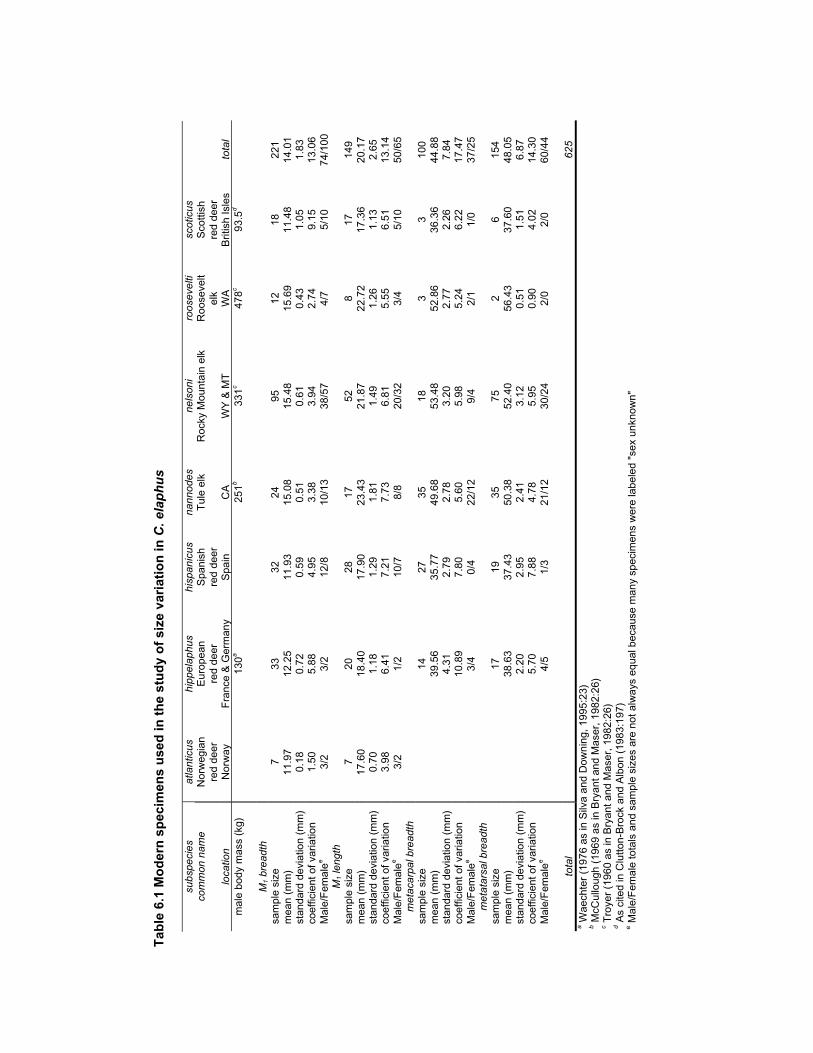
Tab

le 6

.1 M

od

ern

sp

ecim

ens

use

d in

th

e st

ud

y o

f si

ze v

aria

tio

n in

C. e

lap

hu

s

subs

peci

esat

lant

icus

hipp

elap

hus

hisp

anic

usna

nnod

esne

lson

iro

osev

elti

scot

icus

com

mon

nam

eN

orw

egia

nre

d de

erE

urop

ean

red

deer

Spa

nish

red

deer

Tul

e el

kR

ocky

Mou

ntai

n el

kR

oose

velt

elk

Sco

ttish

red

deer

loca

tion

Nor

way

Fra

nce

& G

erm

any

Spa

inC

AW

Y &

MT

WA

Brit

ish

Isle

sto

tal

mal

e bo

dy m

ass

(kg)

130a

251b

331c

478c

93.5

d

M1

brea

dth

sam

ple

size

733

3224

9512

1822

1m

ean

(mm

)11

.97

12.2

511

.93

15.0

815

.48

15.6

911

.48

14.0

1st

anda

rd d

evia

tion

(mm

)0.

180.

720.

590.

510.

610.

431.

051.

83co

effic

ient

of v

aria

tion

1.50

5.88

4.95

3.38

3.94

2.74

9.15

13.0

6M

ale/

Fem

ale

e3/

23/

212

/810

/13

38/5

74/

75/

1074

/100

M1

leng

thsa

mpl

e si

ze7

2028

1752

817

149

mea

n (m

m)

17.6

018

.40

17.9

023

.43

21.8

722

.72

17.3

620

.17

stan

dard

dev

iatio

n (m

m)

0.70

1.18

1.29

1.81

1.49

1.26

1.13

2.65

coef

ficie

nt o

f var

iatio

n3.

986.

417.

217.

736.

815.

556.

5113

.14

Mal

e/F

emal

ee

3/2

1/2

10/7

8/8

20/3

23/

45/

1050

/65

met

acar

pal b

read

thsa

mpl

e si

ze14

2735

183

310

0m

ean

(mm

)39

.56

35.7

749

.68

53.4

852

.86

36.3

644

.88

stan

dard

dev

iatio

n (m

m)

4.31

2.79

2.78

3.20

2.77

2.26

7.84

coef

ficie

nt o

f var

iatio

n10

.89

7.80

5.60

5.98

5.24

6.22

17.4

7M

ale/

Fem

ale

e3/

40/

422

/12

9/4

2/1

1/0

37/2

5m

etat

arsa

l bre

adth

sam

ple

size

1719

3575

26

154

mea

n (m

m)

38.6

337

.43

50.3

852

.40

56.4

337

.60

48.0

5st

anda

rd d

evia

tion

(mm

)2.

202.

952.

413.

120.

511.

516.

87co

effic

ient

of v

aria

tion

5.70

7.88

4.78

5.95

0.90

4.02

14.3

0M

ale/

Fem

ale

e4/

51/

321

/12

30/2

42/

02/

060

/44

tota

l62

5

a W

aech

ter

(197

6 as

in S

ilva

and

Dow

ning

, 199

5:23

)

b M

cCul

loug

h (1

969

as in

Bry

ant a

nd M

aser

, 198

2:26

)

c T

roye

r (1

960

as in

Bry

ant a

nd M

aser

, 198

2:26

)

d A

s ci

ted

in C

lutto

n-B

rock

and

Alb

on (

1983

:197

)

e Mal

e/F

emal

e to

tals

and

sam

ple

size

s ar

e no

t alw

ays

equa

l bec

ause

man

y sp

ecim

ens

wer

e la

bele

d "s

ex u

nkno

wn"

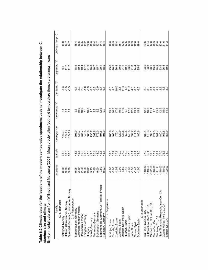
Tab

le 6

.2 C

limat

ic d

ata

for

the

loca

tio

ns

of

the

mo

der

n c

om

par

ativ

e sp

ecim

ens

use

d t

o in

vest

igat

e th

e re

lati

on

ship

bet

wee

n C

.el

aph

us

size

an

d c

limat

eE

nviro

nmen

tal d

ata

are

from

Will

mot

t and

Mat

suur

a (2

001)

. Mea

n pr

ecip

itatio

n (p

pt)

and

tem

pera

ture

(te

mp)

are

ann

ual m

eans

.

loca

lity

long

itude

latit

ude

mea

n pp

t mm

mea

n te

mp

˚CJa

n te

mp

˚CJu

ly te

mp

˚CJu

ly-J

an te

mp

˚CC

. e. a

tlant

icus

Bat

nfjo

rd, N

orw

ay8.

0063

.013

65.6

2.1

-4.3

9.7

14.0

Hitt

eren

(H

itra

Isla

nd),

Nor

way

9.00

63.5

1343

.23.

1-3

.511

.214

.7S

uren

dal (

Sur

nada

l), N

ordm

ore,

Nor

way

9.00

63.0

1343

.23.

1-3

.511

.214

.7C

. e. h

ippe

laph

usB

eben

haus

en, G

erm

any

9.05

48.6

691.

09.

30.

118

.518

.4C

atin

eau

Fro

ntie

r, F

ranc

e2.

5046

.573

4.7

10.9

2.9

19.4

16.5

Dom

inqu

in, F

ranc

e2.

5046

.573

4.7

10.9

2.9

19.4

16.5

Eni

ngen

, Ger

man

y9.

5048

.584

0.5

7.8

-1.0

17.2

18.2

Hun

gary

19.0

047

.056

3.0

10.8

-0.9

21.9

22.8

Ilsfe

ld, G

erm

any

9.25

49.3

736.

79.

50.

818

.818

.0M

onre

pos,

Ger

man

y7.

4550

.469

2.8

8.2

0.3

16.7

16.4

Sch

onbu

ch, G

erm

any

9.00

48.0

772.

06.

6-2

.015

.717

.7S

igis

mon

d de

Cle

rmon

t, La

Ten

aille

, Fra

nce

-0.5

045

.579

7.8

12.6

5.7

20.1

14.4

Tub

inge

n, G

erm

any

9.03

48.5

691.

09.

30.

118

.518

.4C

. e. h

ispa

nicu

sA

nduj

ar, S

pain

-4.0

038

.048

5.6

15.3

6.6

25.6

19.0

Caz

orla

, Spa

in-3

.00

37.7

403.

516

.58.

026

.518

.5C

ordo

ba, S

pain

-4.0

837

.147

6.4

17.6

10.0

26.4

16.4

Cue

nca,

Spa

in-2

.00

40.0

629.

910

.92.

820

.918

.1D

onan

a N

at'l

Par

k, S

pain

-6.5

037

.053

3.8

17.6

11.5

24.1

12.6

Hue

sca,

Spa

in-0

.42

42.0

652.

59.

81.

519

.117

.6Is

la C

ristin

a, S

pain

-7.3

037

.344

3.5

17.3

11.3

23.6

12.3

Jaca

, Spa

in-0

.55

42.1

639.

712

.64.

521

.817

.3Q

uint

o, S

pain

-0.4

841

.141

7.6

15.2

6.8

24.4

17.6

Sou

ther

n S

pain

-4.0

038

.048

5.6

15.3

6.6

25.6

19.0

C. e

. nan

node

sB

ig P

ine,

Inyo

Co.

, CA

-118

.30

37.2

180.

412

.52.

923

.520

.6B

utto

nwill

ow, K

ern

Co.

, CA

-119

.50

35.4

179.

313

.33.

923

.319

.4M

itche

ll F

lat,

Col

usa

Co.

, CA

-122

.50

39.0

899.

111

.13.

120

.117

.0M

ono

Co.

, CA

-118

.87

37.9

427.

39.

30.

919

.818

.9M

onte

rey

Co.

, CA

-121

.31

36.2

389.

413

.88.

118

.910

.8N

ear

Tin

amah

a R

esev

oir,

Inyo

Co.

, CA

-118

.00

37.0

180.

412

.52.

923

.520

.6O

wen

s V

alle

y, In

yo C

o., C

A-1

18.0

036

.516

3.8

15.0

4.8

26.4

21.6

Sol

ano

Co.

, CA

-122

.00

38.0

658.

914

.48.

219

.511

.3

Tab

le 6

.2 c

on

’tlo

calit

ylo

ngitu

dela

titud

em

ean

ppt m

mm

ean

tem

p ˚C

Jan

tem

p ˚C

July

tem

p ˚C

July

-Jan

tem

p ˚C

C. e

. nel

soni

Boz

eman

, MT

-111

.00

45.7

367.

06.

1-6

.319

.025

.3E

stes

Par

k, L

arim

er C

o., C

O-1

05.5

040

.436

7.6

-2.0

-12.

49.

321

.7G

ardi

ner,

Par

k C

o., M

T-1

10.0

045

.021

2.5

2.3

-9.0

14.2

23.2

Idah

o/W

yom

-111

.00

43.0

486.

13.

5-8

.816

.225

.0Ja

ckso

n, W

Y-1

11.0

043

.544

7.8

4.3

-8.3

17.1

25.4

Mis

soul

a C

o., M

T-1

14.0

046

.535

3.9

5.0

-5.7

16.1

21.8

Rio

Bla

nco

Co.

, CO

-108

.00

40.0

351.

17.

4-5

.520

.526

.0S

ande

rs C

o., M

T-1

15.0

047

.568

6.2

1.5

-9.5

13.1

22.6

Yel

low

ston

e N

atl P

ark,

WY

-110

.50

44.5

491.

10.

6-1

0.7

12.5

23.2

C. e

. roo

seve

ltiG

ray'

s H

arbo

r C

o., W

A-1

23.5

047

.526

89.2

1.8

-4.4

8.4

12.8

Hoh

Riv

er, J

effe

rson

Co.

, WA

-124

.00

48.0

2240

.68.

43.

613

.29.

6H

umbo

lt C

o., C

A-1

24.0

041

.018

19.5

11.5

6.9

16.3

9.4

Oric

k, H

umbo

lt C

o., C

A-1

24.0

041

.318

19.2

8.0

4.0

12.3

8.3

Qua

tsin

o, V

anco

uver

Isla

nd, B

. C.

-128

.00

50.5

2440

.58.

74.

013

.99.

9C

. e. s

cotic

usB

alm

acaa

n, In

vern

ess,

Sco

tland

-4.2

557

.588

2.4

4.9

-0.3

10.8

11.1

Bal

mor

al, A

berd

eens

hire

, Sco

tland

-3.0

057

.082

0.8

5.8

0.3

12.1

11.8

Exm

oor,

Dev

on, E

ngla

nd-3

.83

51.0

1142

.09.

95.

015

.810

.8F

t. W

illia

m, S

cotla

nd-5

.12

56.8

2041

.69.

03.

814

.110

.3G

len

Quo

ich,

Inve

rnes

s-sh

ire, S

cotla

nd-5

.25

57.0

1720

.24.

90.

110

.410

.3R

hum

, Sco

tland

-6.3

057

.017

03.9

7.9

3.7

12.3

8.6

The

tford

, Hor

folk

, Eng

land

0.75

52.4

591.

29.

83.

516

.713

.2

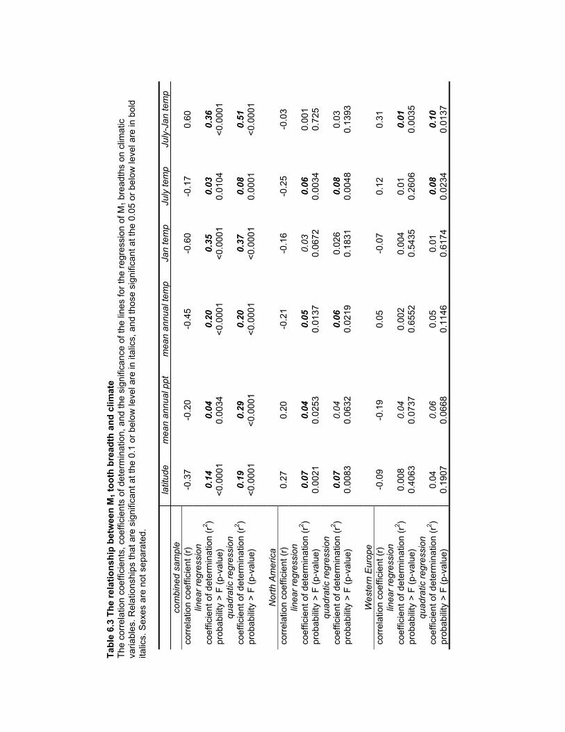
Tab

le 6

.3 T

he

rela

tio

nsh

ip b

etw

een

M1

too

th b

read

th a

nd

clim

ate

The

cor

rela

tion

coef

ficie

nts,

coe

ffici

ents

of d

eter

min

atio

n, a

nd th

e si

gnifi

canc

e of

the

lines

for

the

regr

essi

on o

f M1

brea

dths

on

clim

atic

varia

bles

. Rel

atio

nshi

ps th

at a

re s

igni

fican

t at t

he 0

.1 o

r be

low

leve

l are

in it

alic

s, a

nd th

ose

sign

ifica

nt a

t the

0.0

5 or

bel

ow le

vel a

re in

bol

dita

lics.

Sex

es a

re n

ot s

epar

ated

.

latit

ude

mea

n an

nual

ppt

mea

n an

nual

tem

pJa

n te

mp

July

tem

pJu

ly-J

an te

mp

com

bine

d sa

mpl

eco

rrel

atio

n co

effic

ient

(r)

-0.3

7-0

.20

-0.4

5-0

.60

-0.1

70.

60lin

ear

regr

essi

onco

effic

ient

of d

eter

min

atio

n (r

2 )0.

140.

040.

200.

350.

030.

36pr

obab

ility

> F

(p-

valu

e)<

0.00

010.

0034

<0.

0001

<0.

0001

0.01

04<

0.00

01qu

adra

tic r

egre

ssio

nco

effic

ient

of d

eter

min

atio

n (r

2 )0.

190.

290.

200.

370.

080.

51pr

obab

ility

> F

(p-

valu

e)<

0.00

01<

0.00

01<

0.00

01<

0.00

010.

0001

<0.

0001

Nor

th A

mer

ica

corr

elat

ion

coef

ficie

nt (

r)0.

270.

20-0

.21

-0.1

6-0

.25

-0.0

3lin

ear

regr

essi

onco

effic

ient

of d

eter

min

atio

n (r

2 )0.

070.

040.

050.

030.

060.

001

prob

abili

ty >

F (

p-va

lue)

0.00

210.

0253

0.01

370.

0672

0.00

340.

725

quad

ratic

reg

ress

ion

coef

ficie

nt o

f det

erm

inat

ion

(r2 )

0.07

0.04

0.06

0.02

60.

080.

03pr

obab

ility

> F

(p-

valu

e)0.

0083

0.06

320.

0219

0.18

310.

0048

0.13

93

Wes

tern

Eur

ope

corr

elat

ion

coef

ficie

nt (

r)-0

.09

-0.1

90.

05-0

.07

0.12

0.31

linea

r re

gres

sion

coef

ficie

nt o

f det

erm

inat

ion

(r2 )

0.00

80.

040.

002

0.00

40.

010.

01pr

obab

ility

> F

(p-

valu

e)0.

4063

0.07

370.

6552

0.54

350.

2606

0.00

35qu

adra

tic r

egre

ssio

nco

effic

ient

of d

eter

min

atio

n (r

2 )0.

040.

060.

050.

010.

080.

10pr

obab

ility

> F

(p-

valu

e)0.

1907

0.06

680.

1146

0.61

740.

0234

0.01

37

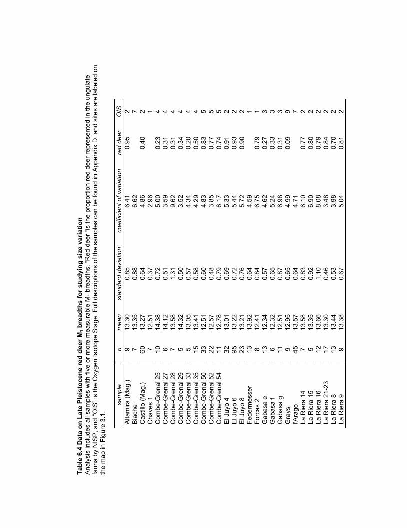
Tab

le 6

.4 D

ata

on

Lat

e P

leis

toce

ne

red

dee

r M

1 b

read

ths

for

stu

dyi

ng

siz

e va

riat

ion

Ana

lysi

s in

clud

es a

ll sa

mpl

es w

ith fi

ve o

r m

ore

mea

sura

ble

M1

brea

dths

. “R

ed d

eer

“is th

e pr

opor

tion

red

deer

rep

rese

nted

in th

e un

gula

tefa

una

by N

ISP

, and

“O

IS”

is th

e O

xyge

n Is

otop

e S

tage

. Ful

l des

crip

tions

of t

he s

ampl

es c

an b

e fo

und

in A

ppen

dix

D, a

nd s

ites

are

labe

led

onth

e m

ap in

Fig

ure

3.1.

sam

ple

nm

ean

stan

dard

dev

iatio

nco

effic

ient

of v

aria

tion

red

deer

OIS

Alta

mira

(M

ag.)

913

.30

0.85

6.41

0.95

2B

iach

e7

13.3

50.

886.

627

Cas

tillo

(M

ag.)

6013

.27

0.64

4.86

0.40

2C

have

s 1

712

.51

0.37

2.96

1C

ombe

-Gre

nal 2

510

14.3

80.

725.

000.

234

Com

be-G

rena

l 27

614

.12

0.51

3.59

0.31

4C

ombe

-Gre

nal 2

87

13.5

81.

319.

620.

314

Com

be-G

rena

l 29

514

.32

0.50

3.52

0.34

4C

ombe

-Gre

nal 3

35

13.0

50.

574.

340.

204

Com

be-G

rena

l 35

1513

.41

0.58

4.29

0.50

4C

ombe

-Gre

nal 5

033

12.5

10.

604.

830.

835

Com

be-G

rena

l 52

2212

.57

0.48

3.85

0.77

5C

ombe

-Gre

nal 5

411

12.7

80.

796.

170.

745

El J

uyo

432

13.0

10.

695.

330.

912

El J

uyo

695

13.2

20.

725.

440.

932

El J

uyo

823

13.2

10.

765.

720.

902

Fed

erm

esse

r13

13.9

20.

644.

591

For

cas

28

12.4

10.

846.

750.

791

Gab

asa

e13

12.3

40.

574.

620.

273

Gab

asa

f6

12.3

20.

655.

240.

333

Gab

asa

g11

12.5

10.

876.

980.

313

Gra

ys9

12.9

50.

654.

990.

099

l'Ara

go45

13.5

70.

644.

717

La R

iera

14

713

.58

0.83

6.10

0.77

2La

Rie

ra 1

55

13.3

50.

926.

900.

802

La R

iera

16

1213

.66

1.10

8.08

0.79

2La

Rie

ra 2

1-23

1713

.30

0.46

3.48

0.84

2La

Rie

ra 8

1313

.44

0.53

3.98

0.70

2La

Rie

ra 9

913

.38

0.67

5.04

0.81

2

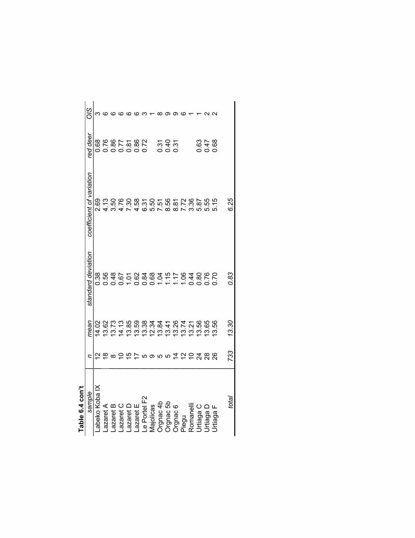
Tab

le 6

.4 c

on

’tsa

mpl

en

mea

nst

anda

rd d

evia

tion

coef

ficie

nt o

f var

iatio

nre

d de

erO

ISLa

beko

Kob

a IX

1214

.02

0.38

2.69

0.68

3La

zare

t A18

13.6

20.

564.

130.

766

Laza

ret B

813

.73

0.48

3.50

0.86

6La

zare

t C10

14.1

30.

674.

760.

776

Laza

ret D

1513

.85

1.01

7.30

0.81

6La

zare

t E17

13.5

90.

624.

580.

866

Le P

orte

l F2

513

.38

0.84

6.31

0.72

3M

ajol

icas

912

.34

0.68

5.50

1O

rgna

c 4b

513

.84

1.04

7.51

0.31

8O

rgna

c 5b

513

.41

1.15

8.56

0.40

9O

rgna

c 6

1413

.26

1.17

8.81

0.31

9P

iegu

1213

.74

1.06

7.72

6R

oman

elli

1013

.21

0.44

3.36

1U

rtia

ga C

2413

.56

0.80

5.87

0.63

1U

rtia

ga D

2813

.65

0.76

5.55

0.47

2U

rtia

ga F

2613

.56

0.70

5.15

0.68

2

tota

l73

313

.30

0.83

6.25

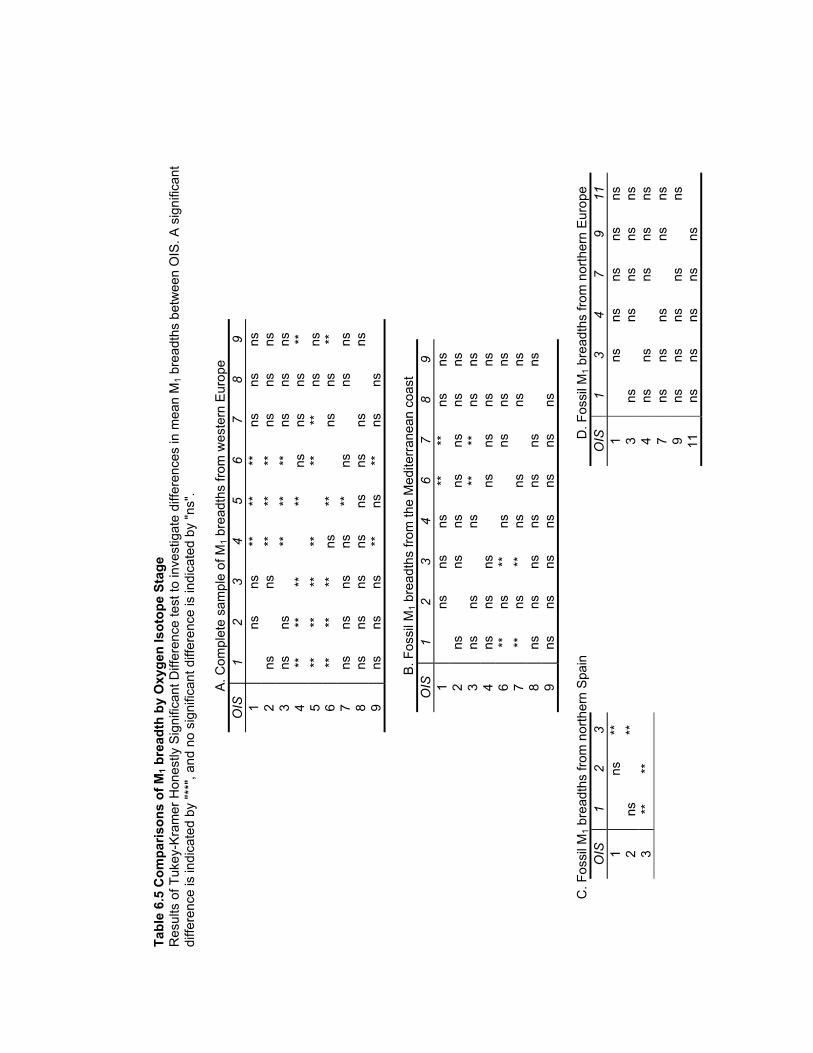
Tab

le 6

.5 C

om

par

iso

ns

of

M1

bre

adth

by

Oxy

gen

Iso

top

e S

tag

eR

esul

ts o

f Tuk

ey-K

ram

er H

ones

tly S

igni

fican

t Diff

eren

ce te

st to

inve

stig

ate

diffe

renc

es in

mea

n M

1 br

eadt

hs b

etw

een

OIS

. A s

igni

fican

tdi

ffere

nce

is in

dica

ted

by "

**",

and

no

sign

ifica

nt d

iffer

ence

is in

dica

ted

by "

ns".

A. C

ompl

ete

sam

ple

of M

1 br

eadt

hs fr

om w

este

rn E

urop

eO

IS1

23

45

67

89

1ns

ns**

****

nsns

ns2

nsns

****

**ns

nsns

3ns

ns**

****

nsns

ns4

****

****

nsns

ns**

5**

****

****

**ns

ns6

****

**ns

**ns

ns**

7ns

nsns

ns**

nsns

ns8

nsns

nsns

nsns

nsns

9ns

nsns

**ns

**ns

ns

B. F

ossi

l M1

brea

dths

from

the

Med

iterr

anea

n co

ast

OIS

12

34

67

89

1ns

nsns

****

nsns

2ns

nsns

nsns

nsns

3ns

nsns

****

nsns

4ns

nsns

nsns

nsns

6**

ns**

nsns

nsns

7**

ns**

nsns

nsns

8ns

nsns

nsns

nsns

9ns

nsns

nsns

nsns

C. F

ossi

l M1

brea

dths

from

nor

ther

n S

pain

D. F

ossi

l M1

brea

dths

from

nor

ther

n E

urop

eO

IS1

23

OIS

13

47

911

1ns

**1

nsns

nsns

ns2

ns**

3ns

nsns

nsns

3**

**4

nsns

nsns

ns7

nsns

nsns

ns9

nsns

nsns

ns11

nsns

nsns

ns

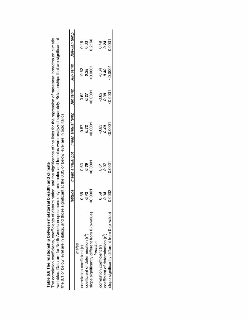
Tab

le 6

.6 T

he

rela

tio

nsh

ip b

etw

een

met

atar

sal b

read

th a

nd

clim

ate

The

cor

rela

tion

coef

ficie

nts,

coe

ffici

ents

of d

eter

min

atio

n, a

nd th

e si

gnifi

canc

e of

the

lines

for

the

regr

essi

on o

f met

atar

sal b

read

ths

on c

limat

icva

riabl

es. D

ata

are

for

Nor

th A

mer

ican

spe

cim

ens

only

, and

mal

es a

nd fe

mal

es w

ere

anal

yzed

sep

arat

ely.

Rel

atio

nshi

ps th

at a

re s

igni

fican

t at

the

0.1

or b

elow

leve

l are

in it

alic

s, a

nd th

ose

sign

ifica

nt a

t the

0.0

5 or

bel

ow le

vel a

re in

bol

d ita

lics.

latit

ude

mea

n an

nual

ppt

mea

n an

nual

tem

pJa

n te

mp

July

tem

pJu

ly-J

an te

mp

mal

esco

rrel

atio

n co

effic

ient

(r)

0.65

0.63

-0.5

7-0

.52

-0.6

20.

18co

effic

ient

of d

eter

min

atio

n (r

2 )0.

420.

390.

320.

270.

380.

03sl

ope

sign

ifica

ntly

diff

eren

t fro

m 0

(p-

valu

e)<

0.00

01<

0.00

01<

0.00

01<

0.00

01<

0.00

010.

2166

fem

ales

corr

elat

ion

coef

ficie

nt (

r)0.

590.

61-0

.63

-0.6

2-0

.64

0.49

coef

ficie

nt o

f det

erm

inat

ion

(r2 )

0.34

0.37

0.40

0.39

0.40

0.24

slop

e si

gnifi

cant

ly d

iffer

ent f

rom

0 (

p-va

lue)

0.00

020.

0001

<0.

0001

<0.

0001

<0.

0001

0.00

31

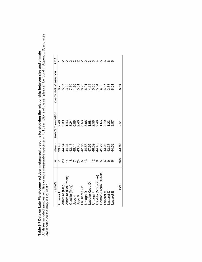
Tab

le 6

.7 D

ata

on

Lat

e P

leis

toce

ne

red

dee

r m

etac

arp

al b

read

ths

for

stu

dyi

ng

th

e re

lati

on

ship

bet

wee

n s

ize

and

clim

ate

Ana

lyse

s in

clud

ed s

ampl

es w

ith fi

ve o

r m

ore

mea

sura

ble

spec

imen

s. F

ull d

escr

iptio

ns o

f the

sam

ples

can

be

foun

d in

App

endi

x D

, an

d si

tes

are

labe

led

on th

e m

ap in

Fig

ure

3.1.

sam

ple

nm

ean

stan

dard

dev

iatio

nco

effic

ient

of v

aria

tion

OIS

Cha

ves

I7

39.4

62.

466.

251

Alta

mira

(M

ag)

2044

.54

2.39

5.37

2A

ltam

ira (

Sol

utre

an)

1444

.31

1.43

3.22

2C

astil

lo (

Mag

)18

43.1

53.

247.

502

Juyo

47

45.1

40.

861.

902

Juyo

624

43.4

62.

405.

512

La R

iera

9-1

15

42.8

53.

538.

232

Urt

iaga

D13

44.5

83.

086.

912

Labe

ko K

oba

IX11

47.9

51.

984.

143

Urt

iaga

F12

46.0

92.

565.

553

Cas

tillo

(M

oust

eria

n)9

44.4

82.

465.

544

Com

be-G

rena

l 50-

50a

541

.22

1.66

4.03

5La

zare

t A6

43.0

42.

796.

476

Laza

ret D

943

.36

1.23

2.83

6La

zare

t E6

44.5

23.

578.

016

tota

l16

644

.09

2.91

6.61

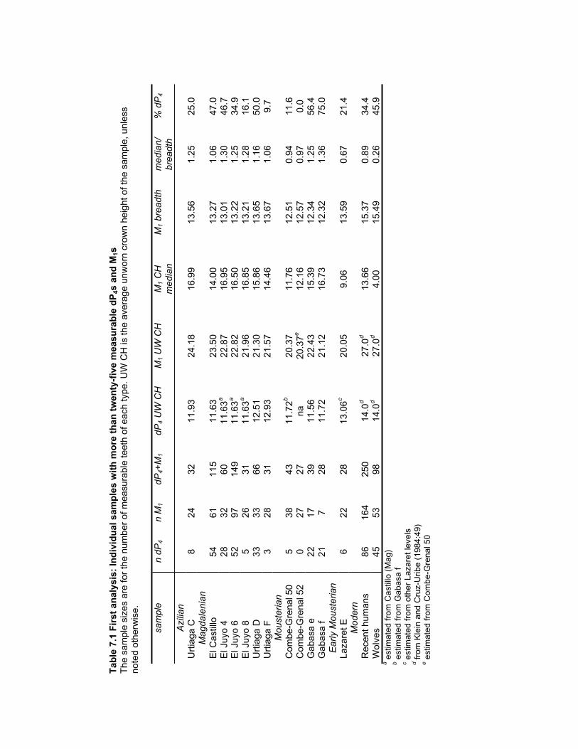
Tab

le 7

.1 F

irst

an

alys

is:

Ind

ivid

ual

sam

ple

s w

ith

mo

re t

han

tw

enty

-fiv

e m

easu

rab

le d

P4s

an

d M

1sT

he s

ampl

e si

zes

are

for

the

num

ber

of m

easu

rabl

e te

eth

of e

ach

type

. UW

CH

is th

e av

erag

e un

wor

n cr

own

heig

ht o

f the

sam

ple,

unl

ess

note

d ot

herw

ise.

sam

ple

n dP

4n

M1

dP4+

M1

dP4

UW

CH

M1

UW

CH

M1

CH

med

ian

M1

brea

dth

med

ian/

brea

dth

% d

P4

Azi

lian

Urt

iaga

C8

2432

11.9

324

.18

16.9

913

.56

1.25

25.0

Mag

dale

nian

El C

astil

lo54

6111

511

.63

23.5

014

.00

13.2

71.

0647

.0E

l Juy

o 4

2832

6011

.63

a22

.87

16.9

513

.01

1.30

46.7

El J

uyo

652

9714

911

.63

a22

.82

16.5

013

.22

1.25

34.9

El J

uyo

85

2631

11.6

3a

21.9

616

.85

13.2

11.

2816

.1U

rtia

ga D

3333

6612

.51

21.3

015

.86

13.6

51.

1650

.0U

rtia

ga F

328

3112

.93

21.5

714

.46

13.6

71.

069.

7M

oust

eria

nC

ombe

-Gre

nal 5

05

3843

11.7

2b

20.3

711

.76

12.5

10.

9411

.6C

ombe

-Gre

nal 5

20

2727

na20

.37

e12

.16

12.5

70.

970.

0G

abas

a e

2217

3911

.56

22.4

315

.39

12.3

41.

2556

.4G

abas

a f

217

2811

.72

21.1

216

.73

12.3

21.

3675

.0E

arly

Mou

ster

ian

Laza

ret E

622

2813

.06

c20

.05

9.06

13.5

90.

6721

.4M

oder

nR

ecen

t hum

ans

8616

425

014

.0d

27.0

d13

.66

15.3

70.

8934

.4W

olve

s45

5398

14.0

d27

.0d

4.00

15.4

90.

2645

.9a e

stim

ated

from

Cas

tillo

(M

ag)

b est

imat

ed fr

om G

abas

a f

c est

imat

ed fr

om o

ther

Laz

aret

leve

lsd fr

om K

lein

and

Cru

z-U

ribe

(198

4:49

)e e

stim

ated

from

Com

be-G

rena

l 50

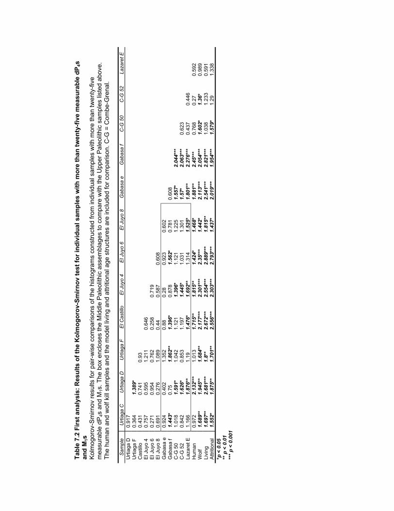
Tab

le 7

.2 F

irst

an

alys

is:

Res

ult

s o

f th

e K

olm

og

oro

v-S

mir

no

v te

st f

or

ind

ivid

ual

sam

ple

s w

ith

mo

re t

han

tw

enty

-fiv

e m

easu

rab

le d

P4s

and

M1s

Kol

mog

orov

-Sm

irnov

res

ults

for

pair-

wis

e co

mpa

rison

s of

the

hist

ogra

ms

cons

truc

ted

from

indi

vidu

al s

ampl

es w

ith m

ore

than

twen

ty-f

ive

mea

sura

ble

dP4s

and

M1s

. The

box

enc

lose

s th

e M

iddl

e P

aleo

lithi

c as

sem

blag

es to

com

pare

with

the

Upp

er P

aleo

lithi

c sa

mpl

es li

sted

abo

ve.

The

hum

an a

nd w

olf k

ill s

ampl

es a

nd th

e m

odel

livi

ng a

nd a

ttriti

onal

age

str

uctu

res

are

incl

uded

for

com

paris

on. C

-G =

Com

be-G

rena

l.

Sam

ple

Urt

iaga

CU

rtia

ga D

Urt

iaga

FE

l Cas

tillo

El J

uyo

4E

l Juy

o 6

El J

uyo

8G

abas

a e

Gab

asa

fC

-G 5

0C

-G 5

2La

zare

t EU

rtia

ga D

0.91

7U

rtia

ga F

0.36

41.

389*

Cas

tillo

0.43

10.

741

0.93

El J

uyo

40.

757

0.59

51.

211

0.64

6E

l Juy

o 6

0.27

10.

954

0.76

20.

258

0.71

9E

l Juy

o 8

0.69

10.

276

1.08

90.

440.

587

0.60

8G

abas

a e

0.92

40.

402

1.35

20.

880.

280.

923

0.60

2G

abas

a f

1.44

3*0.

751.

862*

*1.

396*

0.87

81.

562*

0.78

10.

608

C-G

50

1.01

81.

591*

1.04

21.

121

1.39

6*1.

121

1.22

51.

557*

2.04

4***

C-G

52

0.84

21.

626*

0.85

31.

197

1.44

5*1.

031

1.30

11.

57*

2.06

3***

0.62

3La

zare

t E1.

166

1.87

6**

1.19

1.47

6*1.

692*

*1.

314

1.52

5*1.

801*

*2.

276*

**0.

437

0.44

6H

uman

0.97

22.

132*

**1.

013

1.71

5**

1.81

5**

1.42

4*1.

468*

1.88

1**

2.45

***

0.76

80.

270.

592

Wol

f1.

689*

*1.

945*

*1.

684*

*2.

177*

**2.

301*

**2.

35**

*1.

442*

2.11

3***

2.05

4***

1.60

2*1.

36*

0.98

9Li

ving

1.69

7**

2.68

1***

1.8*

*2.

672*

**2.

554*

**2.

889*

**1.

815*

*2.

541*

**2.

821*

**1.

038

1.23

30.

591

Attr

ition

al1.

552*

1.87

5**

1.70

1**

2.55

6***

2.30

3***

2.79

3***

1.43

7*2.

019*

**1.

954*

**1.

579*

1.29

1.33

8*p

< 0

.05

** p

< 0

.01

***

p <

0.0

01

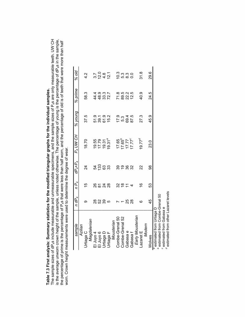
Tab

le 7

.3 F

irst

an

alys

is:

Su

mm

ary

stat

isti

cs f

or

the

mo

dif

ied

tri

ang

ula

r g

rap

hs

for

the

ind

ivid

ual

sam

ple

s.T

he s

ampl

e si

zes

of d

P4s

incl

ude

mea

sura

ble

and

unm

easu

rabl

e sp

ecim

ens,

and

the

sam

ple

size

s of

P4s

are

onl

y m

easu

rabl

e te

eth.

UW

CH

is th

e av

erag

e un

wor

n cr

own

heig

ht o

f the

sam

ple,

unl

ess

note

d ot

herw

ise.

The

per

cent

age

of y

oung

is th

e pe

rcen

tage

of d

P4s

in th

e sa

mpl

e,th

e pe

rcen

tage

of p

rime

is th

e pe

rcen

tage

of P

4s th

at w

ere

less

than

hal

f wor

n, a

nd th

e pe

rcen

tage

of o

ld is

of t

eeth

that

wer

e m

ore

than

hal

fw

orn.

Cro

wn

heig

ht m

easu

rem

ents

wer

e us

ed to

det

erm

ine

the

degr

ee o

f wea

r.

sam

ple

n dP

4n

P4

dP4+

P4

P4

UW

CH

% y

oung

% p

rime

% o

ldA

zilia

nU

rtia

ga C

915

2418

.70

37.5

58.3

4.2

Mag

dale

nian

El J

uyo

428

2654

19.5

551

.944

.43.

7E

l Juy

o 6

5281

133

17.7

939

.148

.912

.0U

rtia

ga D

3924

6319

.31

61.9

33.3

4.8

Urt

iaga

F5

2833

19.3

1a

15.2

72.7

12.1

Mou

ster

ian

Com

be-G

rena

l 50

732

3917

.65

17.9

71.8

10.3

Com

be-G

rena

l 52

118

1917

.65

b5.

389

.55.

3G

abas

a e

2511

3617

.77

69.4

22.2

8.3

Gab

asa

f28

432

17.7

7c

87.5

12.5

0.0

Ear

ly M

oust

eria

nLa

zare

t E6

1622

19.7

7d

27.3

40.9

31.8

Mod

ern

Wol

ves

4553

9823

.045

.924

.529

.6a e

stim

ated

from

Urt

iaga

Db e

stim

ated

from

Com

be-G

rena

l 50

c est

imat

ed fr

om G

abas

a e

d est

imat

ed fr

om o

ther

Laz

aret

leve

ls

Tab

le 7

.4 S

eco

nd

an

alys

is:

Gro

up

ed s

amp

les

wit

h m

ore

th

an t

wen

ty-f

ive

mea

sura

ble

dP

4s a

nd

M1s

The

sam

ple

size

s ar

e fo

r th

e nu

mbe

r of

mea

sura

ble

teet

h of

eac

h ty

pe. U

W C

H is

the

aver

age

unw

orn

crow

n he

ight

of t

he s

ampl

e, u

nles

sno

ted

othe

rwis

e.

sam

ple

n dP

4n

M1

dP4+

M1

dP4

UW

CH

M1

UW

CH

M1

CH

med

ian

M1

brea

dth

med

ian/

brea

dth

% d

P4

Azi

lian

N. S

pani

sh A

zilia

n8

4149

11.9

323

.02

16.9

013

.12

1.29

16.3

Mag

dale

nian

El C

astil

lo54

6111

511

.63

23.5

014

.00

13.2

71.

0647

.0E

l Juy

o85

155

240

11.9

322

.64

16.7

013

.18

1.27

35.4

Urt

iaga

3564

9912

.52

21.4

314

.48

13.6

41.

0635

.4S

olut

rean

La R

iera

2248

7012

.77

21.8

615

.44

13.4

91.

1431

.4M

oust

eria

nG

abas

a60

3898

11.7

121

.86

16.4

712

.53

1.31

61.2

Com

be-G

rena

l 1-3

59

7382

11.4

526

.15

9.50

13.8

80.

6811

.0C

ombe

-Gre

nal 3

6-54

1097

107

11.7

1a

20.5

811

.10

12.7

60.

879.

3E

arly

Mou

ster

ian

Laza

ret

2573

9813

.06

21.8

08.

8413

.75

0.64

25.5

Mod

ern

Rec

ent h

uman

s86

164

250

14.0

b27

.0b

13.6

615

.37

0.89

34.4

Wol

ves

4553

9814

.0b

27.0

b4.

0015

.49

0.26

45.9

a est

imat

ed fr

om G

abas

ab fr

om K

lein

and

Cru

z-U

ribe

(198

4:49

)

Tab

le 7

.5 S

eco

nd

an

alys

is:

Res

ult

s o

f th

e K

olm

og

oro

v-S

mir

no

v te

st f

or

gro

up

ed s

amp

les

wit

h m

ore

th

an t

wen

ty-f

ive

mea

sura

ble

dP

4s a

nd

M1s

Kol

mog

orov

-Sm

irnov

res

ults

for

pair-

wis

e co

mpa

rison

s of

the

hist

ogra

ms

cons

truc

ted

from

gro

uped

sam

ples

with

mor

e th

an tw

enty

-fiv

em

easu

rabl

e dP

4s a

nd M

1s. T

he b

ox e

nclo

ses

the

Mid

dle

to U

pper

Pal

eolit

hic

com

paris

ons.

(C

-G =

Com

be-G

rena

l)

A. C

ompl

ete

age

dist

ribut

ion

sam

ple

N S

pani

sh A

zE

l Cas

tillo

El J

uyo

Urt

iaga

La R

iera

Gab

asa

C-G

1-3

5C

-G 3

6-54

Laza

ret

El C

astil

lo0.

84E

l Juy

o0.

721

0.39

2U

rtia

ga0.

595

0.40

80.

565

La R

iera

1.09

20.

430.

641

0.68

9G

abas

a0.

877

1.45

8*1.

709*

*1.

74**

1.57

3*C

-G 1

-35

3.24

1***

3.07

9***

3.58

9***

3.17

9***

2.14

7***

4.23

7***

C-G

36-

542.

057*

**1.

867*

*1.

988*

**1.

791*

*1.

198

3.21

4***

1.71

2**

Laza

ret

2.23

7***

2.02

7***

2.47

***

2.00

3***

1.42

5*3.

188*

**1.

293

0.91

3H

uman

s1.

745*

*1.

715*

*1.

862*

*1.

417*

0.94

43.

278*

**2.

924*

**1.

015

2.05

***

Wol

f2.

251*

**2.

177*

**2.

809*

**2.

005*

**1.

768*

*2.

912*

**2.

146*

**2.

029*

**1.

395*

Livi

ng2.

754*

**2.

672*

**3.

702*

**2.

74**

*1.

512*

4.22

5***

1.64

4**

1.48

8*0.

368

Attr

ition

al2.

199*

**2.

556*

**3.

653*

**1.

997*

**1.

871*

*3.

145*

**3.

099*

**2.

26**

*1.

893*

*

B. A

dults

onl

y. A

ge c

lass

1 w

as d

elet

ed. S

ampl

e si

zes

wer

e to

o sm

all t

o co

mpa

re th

e no

rthe

rn S

pani

sh A

zilia

n an

d G

abas

a sa

mpl

es.

sam

ple

El C

astil

loE

l Juy

oU

rtia

gaLa

Rie

raC

-G 1

-35

C-G

36-

54La

zare

tE

l Juy

o0.

428

Urt

iaga

0.57

40.

529

La R

iera

0.22

30.

50.

708

C-G

1-3

51.

084

1.63

8**

1.39

*0.

88C

-G 3

6-54

0.33

40.

803

0.91

40.

281

0.85

7La

zare

t0.

973

1.44

3*1.

146

0.74

30.

372

0.74

3H

uman

s0.

211

0.53

10.

755

0.31

1.70

3**

0.70

11.

532*

Wol

ves

1.84

**2.

53**

*1.

779*

*1.

615*

1.40

4*2.

113*

**1.

437*

Livi

ng1.

121

2.11

4***

1.44

7*0.

911

0.39

11.

262

0.29

9A

ttriti

onal

2.33

8***

3.50

3***

2.02

2***

1.87

1**

1.77

4**

2.73

5***

1.70

5**

*p <

0.0

5**

p <

0.0

1**

* p

< 0

.001

Tab

le 7

.6 S

eco

nd

an

alys

is:

Su

mm

ary

stat

isti

cs f

or

the

mo

dif

ied

tri

ang

ula

r g

rap

h f

or

the

gro

up

ed s

amp

les

The

sam

ple

size

s of

dP

4s in

clud

e m

easu

rabl

e an

d un

mea

sura

ble

spec

imen

s, a

nd th

e sa

mpl

e si

zes

of P

4s a

re o

nly

mea

sura

ble

teet

h. U

W C

His

the

aver

age

unw

orn

crow

n he

ight

of t

he s

ampl

e. T

he p

erce

ntag

e of

you

ng is

the

perc

enta

ge o

f dP

4s in

the

sam

ple,

the

perc

enta

ge o

f prim

eis

the

perc

enta

ge o

f P4s

that

wer

e le

ss th

an h

alf w

orn,

and

the

perc

enta

ge o

f old

is o

f tee

th th

at w

ere

mor

e th

an h

alf w

orn.

Cro

wn

heig

htm

easu

rem

ents

wer

e us

ed to

det

erm

ine

the

degr

ee o

f wea

r.

sam

ple

n dP

4n

P4

dP4+

P4

P4

UW

CH

% y

oung

% p

rime

% o

ldA

zilia

nN

. Spa

nish

Azi

lian

1025

3518

.628

.668

.62.

9M

agda

leni

anE

l Juy

o85

107

192

18.3

44.3

45.8

9.9

Urt

iaga

4654

100

19.3

46.0

46.0

8.0

Sol

utre

anLa

Rie

ra29

4271

19.9

40.8

52.1

7.0

Mou

ster

ian

Gab

asa

7521

9617

.878

.116

.75.

2C

ombe

-Gre

nal 1

-35

1167

7819

.214

.155

.130

.8C

ombe

-Gre

nal 3

6-54

1477

9117

.715

.472

.512

.1E

arly

Mou

ster

ian

Laza

ret

2888

116

19.7

24.1

41.4

34.5

Mod

ern

Wol

ves

4553

9823

.045

.924

.529

.6

Tab

le 7

.7 T

hir

d a

nal

ysis

: G

rou

ped

sam

ple

s w

ith

ten

or

mo

re m

easu

rab

le M

1 cr

ow

n h

eig

hts

The

sam

ple

size

s of

dP

4s in

clud

e m

easu

rabl

e an

d un

mea

sura

ble

spec

imen

s, a

nd th

e sa

mpl

e si

zes

of M

1s a

re a

ll m

easu

rabl

e M

1s.

sam

ple

n dP

4n

M1

dP4+

M1

M1

CH

med

ian

M1

brea

dth

med

ian/

brea

dth

% d

P4

Hol

ocen

eG

erm

an F

eder

mes

ser

514

1915

.62

13.9

21.

1226

.32

N. S

pani

sh A

zilia

n10

4151

16.9

013

.12

1.29

19.6

1S

tar

Car

r M

esol

ithic

232

3413

.312

.88

1.03

5.88

Mag

dale

nian

Alta

mira

1010

2013

.45

13.3

01.

0150

.00

El C

astil

lo56

6111

714

.00

13.2

71.

0647

.86

El J

uyo

8515

524

016

.70

13.1

81.

2735

.42

La R

iera

516

2115

.00

13.2

71.

1323

.81

Urt

iaga

4664

110

14.4

813

.64

1.06

41.8

2S

olut

rean

Alta

mira

320

2315

.50

13.5

1*1.

1513

.04

La R

iera

2948

7715

.44

13.5

11.

1437

.66

Châ

telp

erro

nian

Labe

ko K

oba

IX in

f.2

1214

16.8

514

.02

1.20

14.2

9M

oust

eria

nG

abas

a75

3811

316

.47

12.5

31.

3166

.37

Com

be-G

rena

l 1-3

511

7384

9.50

13.8

80.

6813

.10

Com

be-G

rena

l 36-

5414

9711

111

.10

12.7

60.

8712

.61

Ear

ly M

oust

eria

nLa

zare

t28

7310

18.

8413

.75

0.64

27.7

2P

iegu

218

2012

.12

13.7

40.

8810

.00

Ach

eulo

-Yab

rudi

anT

abun

210

1211

.55

13.5

80.

8516

.67

Mod

ern

Rec

ent h

uman

s86

164

250

13.6

615

.37

0.89

34.4

0W

olve

s45

5398

4.00

15.4

90.

2645

.92

* es

timat

ed fr

om L

a R

iera

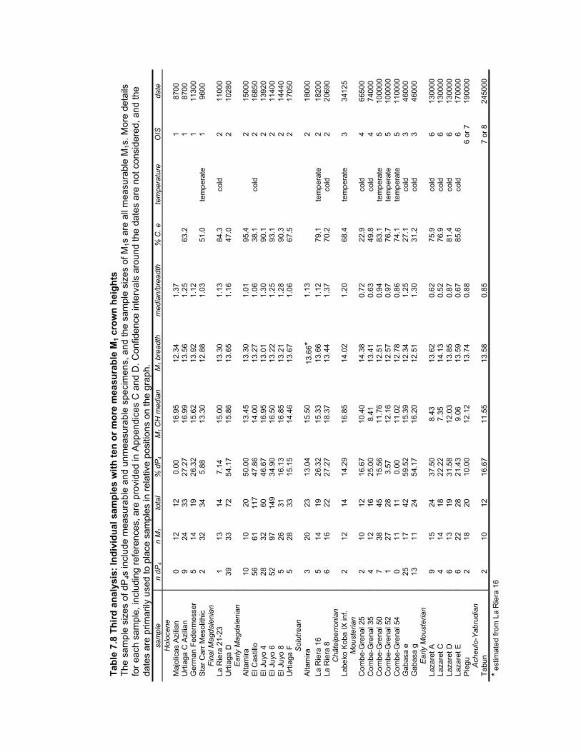
Tab

le 7

.8 T

hir

d a

nal

ysis

: In

div

idu

al s

amp

les

wit

h t

en o

r m

ore

mea

sura

ble

M1

cro

wn

hei

gh

tsT

he s

ampl

e si

zes

of d

P4s

incl

ude

mea

sura

ble

and

unm

easu

rabl

e sp

ecim

ens,

and

the

sam

ple

size

s of

M1s

are

all

mea

sura

ble

M1s

. Mor

e de

tails

for

each

sam

ple,

incl

udin

g re

fere

nces

, are

pro

vide

d in

App

endi

ces

C a

nd D

. Con

fiden

ce in

terv

als

arou

nd th

e da

tes

are

not c

onsi

der

ed, a

nd th

eda

tes

are

prim

arily

use

d to

pla

ce s

ampl

es in

rel

ativ

e po

sitio

ns o

n th

e gr

aph.

sam

ple

n dP

4n

M1

tota

l%

dP

4M

1 C

H m

edia

nM

1 br

eadt

hm

edia

n/br

eadt

h%

C. e

tem

pera

ture

OIS

date

Hol

ocen

eM

ajol

icas

Azi

lian

012

120.

0016

.95

12.3

41.

371

8700

Urt

iaga

C A

zilia

n9

2433

27.2

716

.99

13.5

61.

2563

.21

8700

Ger

man

Fed

erm

esse

r5

1419

26.3

215

.62

13.9

21.

121

1130

0S

tar

Car

r M

esol

ithic

232

345.

8813

.30

12.8

81.

0351

.0te

mpe

rate

196

00F

inal

Mag

dale

nian

La R

iera

21-

231

1314

7.14

15.0

013

.30

1.13

84.3

cold

211

000

Urt

iaga

D39

3372

54.1

715

.86

13.6

51.

1647

.02

1028

0E

arly

Mag

dale

nian

Alta

mira

1010

2050

.00

13.4

513

.30

1.01

95.4

215

000

El C

astil

lo56

6111

747

.86

14.0

013

.27

1.06

38.1

cold

216

850

El J

uyo

428

3260

46.6

716

.95

13.0

11.

3090

.12

1392

0E

l Juy

o 6

5297

149

34.9

016

.50

13.2

21.

2593

.12

1140

0E

l Juy

o 8

526

3116

.13

16.8

513

.21

1.28

90.3

214

440

Urt

iaga

F5

2833

15.1

514

.46

13.6

71.

0667

.52

1705

0S

olut

rean

Alta

mira

320

2313

.04

15.5

013

.66*

1.13

218

000

La R

iera

16

514

1926

.32

15.3

313

.66

1.12

79.1

tem

pera

te2

1820

0La

Rie

ra 8

616

2227

.27

18.3

713

.44

1.37

70.2

cold

220

690

Châ

telp

erro

nian

Labe

ko K

oba

IX in

f.2

1214

14.2

916

.85

14.0

21.

2068

.4te

mpe

rate

334

125

Mou

ster

ian

Com

be-G

rena

l 25

210

1216

.67

10.4

014

.38

0.72

22.9

cold

466

500

Com

be-G

rena

l 35

412

1625

.00

8.41

13.4

10.

6349

.8co

ld4

7400

0C

ombe

-Gre

nal 5

07

3845

15.5

611

.76

12.5

10.

9483

.1te

mpe

rate

510

0000

Com

be-G

rena

l 52

127

283.

5712

.16

12.5

70.

9776

.7te

mpe

rate

510

0000

Com

be-G

rena

l 54

011

110.

0011

.02

12.7

80.

8674

.1te

mpe

rate

511

0000

Gab

asa

e25

1742

59.5

215

.39

12.3

41.

2527

.1co

ld3

4600

0G

abas

a g

1311

2454

.17

16.2

012

.51

1.30

31.2

cold

346

000

Ear

ly M

oust

eria

nLa

zare

t A9

1524

37.5

08.

4313

.62

0.62

75.9

cold

613

0000

Laza

ret C

414

1822

.22

7.35

14.1

30.

5276

.9co

ld6

1300

00La

zare

t D6

1319

31.5

812

.03

13.8

50.

8781

.4co

ld6

1300

00La

zare

t E6

2228

21.4

39.

0613

.59

0.67

85.6

cold

617

0000

Pie

gu2

1820

10.0

012

.12

13.7

40.

886

or 7

1900

00A

cheu

lo-Y

abru

dian

Tab

un2

1012

16.6

711

.55

13.5

80.

857

or 8

2450

00

* es

timat

ed fr

om L

a R

iera

16

192

Appendix B Illustrations

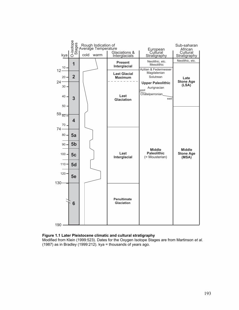
193

Figure 1.1 Later Pleistocene climatic and cultural stratigraphyModified from Klein (1999:523). Dates for the Oxygen Isotope Stages are from Martinson et al.(1987) as in Bradley (1999:212). kya = thousands of years ago.

12

24

59

70

74

90

100

110

120

10

20

30

40

50

60

80

190

6

5e

5d

5c

5b

5a

4

3

2

1

cold warm

Rough Indication ofAverage Temperature

Glaciations &Interglacials

LastInterglacial

LastGlaciation

PresentInterglacial

EuropeanCultural

Stratigraphy

Neolithic, etc.Mesolithic

Upper Paleolithic

west

east

MiddlePaleolithic

(= Mousterian)

PenultimateGlaciation

130

O-is

otop

eS

tage

s

kya

Last GlacialMaximum

Sub-saharanAfricanCultural

Stratigraphy

MiddleStone Age

(MSA)

LateStone Age

(LSA)

Neolithic, etc.

Châtelperronian

Aurignacian

SolutreanMagdalenian

Azilian & Federmesser

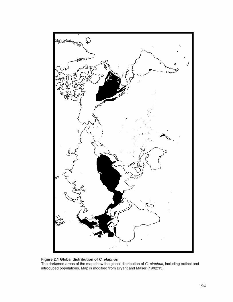
194

Figure 2.1 Global distribution of C. elaphusThe darkened areas of the map show the global distribution of C. elaphus, including extinct andintroduced populations. Map is modified from Bryant and Maser (1982:15).

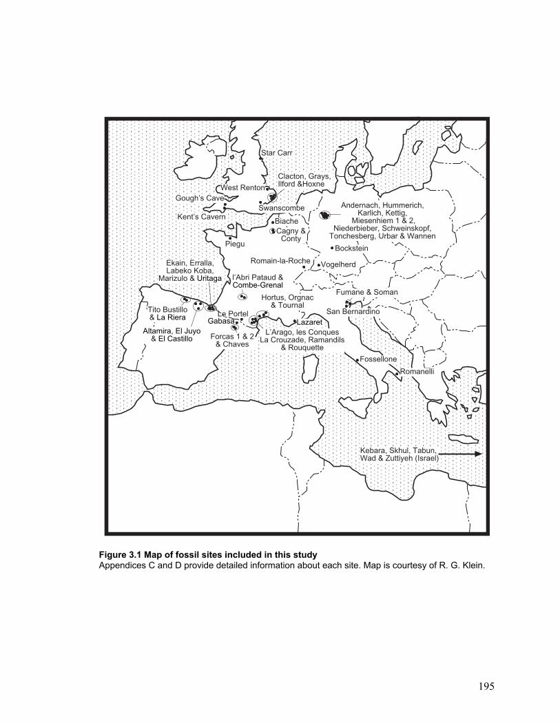
195

l’Abri Pataud &Combe-Grenal

Altamira, El Juyo& El Castillo

Tito Bustillo& La Riera

Ekain, Erralla,Labeko Koba,

Marizulo & Uritaga

Gough’s CaveAndernach, Hummerich,

Karlich, Kettig, Miesenhiem 1 & 2,

Niederbieber, Schweinskopf,Tonchesberg, Urbar & Wannen

Vogelherd

Romanelli

West Renton

Star Carr

Hortus, Orgnac& Tournal

Fumane & Soman

L’Arago, les ConquesLa Crouzade, Ramandils

& Rouquette

LazaretLe Portel

Romain-la-Roche

BiacheCagny &

Conty

Clacton, Grays,Ilford &Hoxne

Kebara, Skhul, Tabun,Wad & Zuttiyeh (Israel)

GabasaSan Bernardino

Fossellone

Forcas 1 & 2& Chaves

SwanscombeKent’s Cavern

BocksteinPiegu

Figure 3.1 Map of fossil sites included in this studyAppendices C and D provide detailed information about each site. Map is courtesy of R. G. Klein.

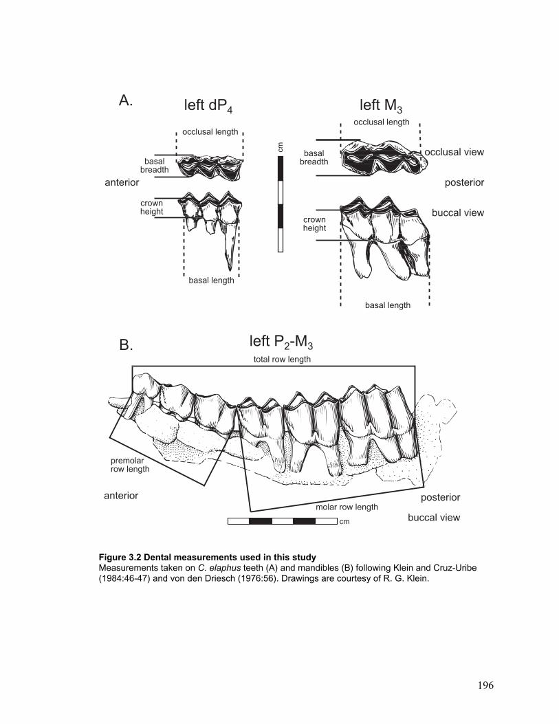
196

Figure 3.2 Dental measurements used in this studyMeasurements taken on C. elaphus teeth (A) and mandibles (B) following Klein and Cruz-Uribe(1984:46-47) and von den Driesch (1976:56). Drawings are courtesy of R. G. Klein.

A.

B.

occlusal length

basalbreadth

crownheight

basal length

occlusal length

basalbreadth

crownheight

basal length

left dP4 left M3

total row length

premolarrow length

molar row length

left P2-M3

cm

cm

anterior

anterior posterior

buccal view

occlusal view

posterior

buccal view

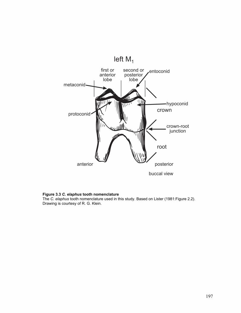
197

Figure 3.3 C. elaphus tooth nomenclatureThe C. elaphus tooth nomenclature used in this study. Based on Lister (1981:Figure 2.2).Drawing is courtesy of R. G. Klein.

anterior posterior

buccal view

crown-rootjunction

crown

root

first oranterior

lobe

second orposterior

lobemetaconid

protoconid

entoconid

hypoconid

left M1

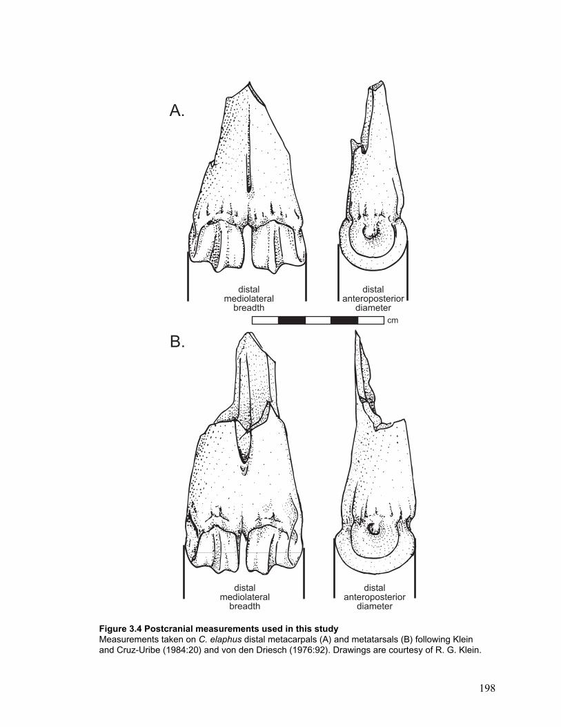
198

Figure 3.4 Postcranial measurements used in this studyMeasurements taken on C. elaphus distal metacarpals (A) and metatarsals (B) following Kleinand Cruz-Uribe (1984:20) and von den Driesch (1976:92). Drawings are courtesy of R. G. Klein.

A.

B.

distalmediolateral

breadth

distalanteroposterior

diameter

distalmediolateral

breadth

distalanteroposterior

diameter

cm

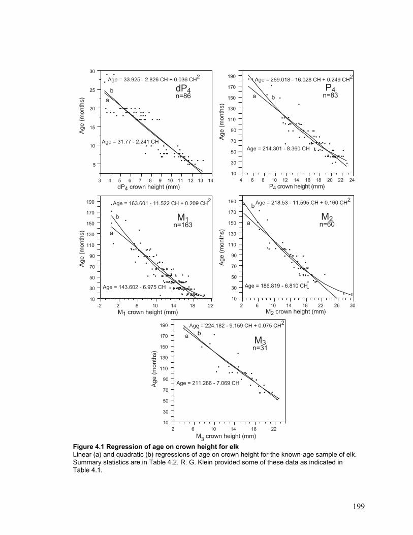
199

Figure 4.1 Regression of age on crown height for elkLinear (a) and quadratic (b) regressions of age on crown height for the known-age sample of elk.Summary statistics are in Table 4.2. R. G. Klein provided some of these data as indicated inTable 4.1.

10

30

50

70

90

110

130

150

170

190

M3 crown height (mm)

Age

(m

onth

s)

a bM3n=31

Age = 211.286 - 7.069 CH

Age = 224.182 - 9.159 CH + 0.075 CH2

Age

(m

onth

s)

10

30

50

70

90

110

130

150

170

190

M1 crown height (mm)

Age

(m

onth

s)

Age

(m

onth

s)

10

30

50

70

90

110

130

150

170

190

P4 crown height (mm)

5

10

15

20

25

30

3 4 5 6 7 8 9 10 11 12 13 14dP4 crown height (mm)

a

b

a

ba b

dP4n=86

P4n=83

M1n=163

Age = 31.77 - 2.241 CH

Age = 33.925 - 2.826 CH + 0.036 CH2

Age = 214.301 - 8.360 CH

Age = 269.018 - 16.028 CH + 0.249 CH2

Age = 143.602 - 6.975 CH

Age = 163.601 - 11.522 CH + 0.209 CH2

10

30

50

70

90

110

130

150

170

190

M2 crown height (mm)

Age

(m

onth

s)a

b

M2n=60

Age = 186.819 - 6.810 CH

Age = 218.53 - 11.595 CH + 0.160 CH2

4 6 8 10 12 14 16 18 20 22 24

-2 2 6 10 14 18 22 2 6 10 14 18 22 26 30

2 6 10 14 18 22

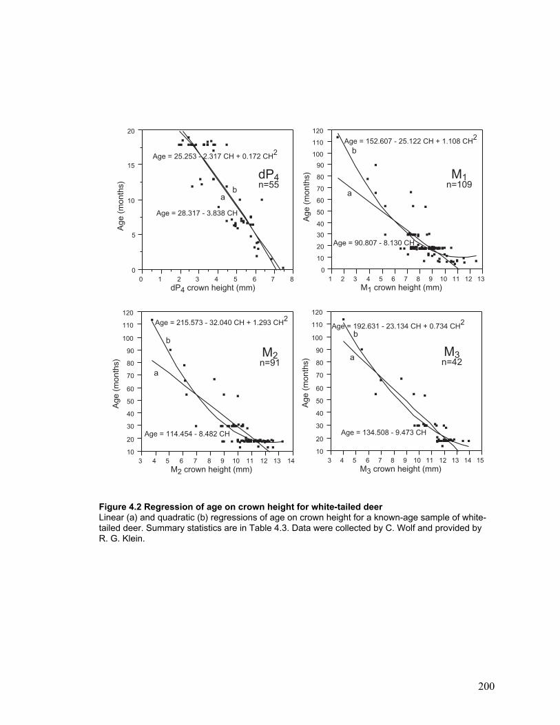
200

Figure 4.2 Regression of age on crown height for white-tailed deerLinear (a) and quadratic (b) regressions of age on crown height for a known-age sample of white-tailed deer. Summary statistics are in Table 4.3. Data were collected by C. Wolf and provided byR. G. Klein.

0

5

10

15

20

0 1 2 3 4 5 6 7 8dP4 crown height (mm)

Age

(m

onth

s)

dP4n=55

ab

Age = 28.317 - 3.838 CH

Age = 25.253 - 2.317 CH + 0.172 CH2

0

10

20

30

40

50

60

70

80

90

100

110

120

1 2 3 4 5 6 7 8 9 10 11 12 13M1 crown height (mm)

Age

(m

onth

s) M1n=109

a

b

Age = 90.807 - 8.130 CH

Age = 152.607 - 25.122 CH + 1.108 CH2

10

20

30

40

50

60

70

80

90

100

110

120

3 4 5 6 7 8 9 10 11 12 13 14 15M3 crown height (mm)

Age

(m

onth

s)

M3n=42a

Age = 192.631 - 23.134 CH + 0.734 CH2

Age = 134.508 - 9.473 CH

b

10

20

30

40

50

60

70

80

90

100

110

120

3 4 5 6 7 8 9 10 11 12 13 14M2 crown height (mm)

Age

(m

onth

s)

M2n=91

a

b

Age = 114.454 - 8.482 CH

Age = 215.573 - 32.040 CH + 1.293 CH2

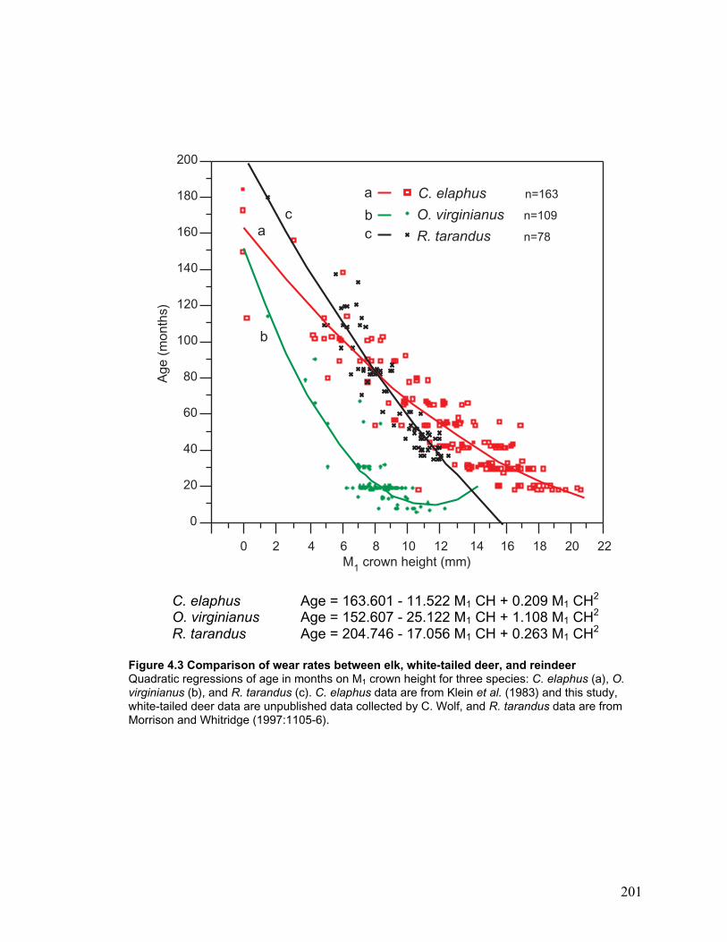
201

C. elaphus Age = 163.601 - 11.522 M1 CH + 0.209 M1 CH2

O. virginianus Age = 152.607 - 25.122 M1 CH + 1.108 M1 CH2

R. tarandus Age = 204.746 - 17.056 M1 CH + 0.263 M1 CH2

Figure 4.3 Comparison of wear rates between elk, white-tailed deer, and reindeerQuadratic regressions of age in months on M1 crown height for three species: C. elaphus (a), O.virginianus (b), and R. tarandus (c). C. elaphus data are from Klein et al. (1983) and this study,white-tailed deer data are unpublished data collected by C. Wolf, and R. tarandus data are fromMorrison and Whitridge (1997:1105-6).

0

20

40

60

80

100

120

140

160

180

200

0 2 4 6 8 10 12 14 16 18 20 22M1 crown height (mm)

Age

(m

onth

s)

C. elaphus n=163

O. virginianus n=109

R. tarandus n=78a

b

c

a

bc

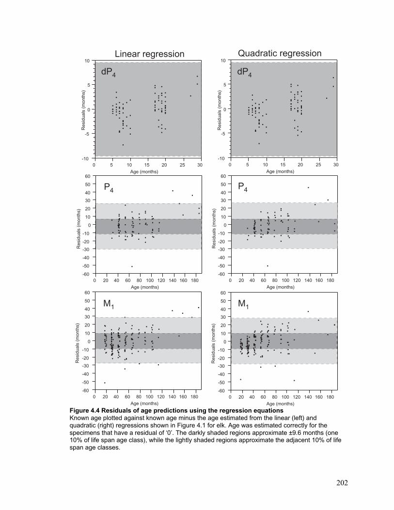
202

Figure 4.4 Residuals of age predictions using the regression equationsKnown age plotted against known age minus the age estimated from the linear (left) andquadratic (right) regressions shown in Figure 4.1 for elk. Age was estimated correctly for thespecimens that have a residual of ‘0’. The darkly shaded regions approximate ±9.6 months (one10% of life span age class), while the lightly shaded regions approximate the adjacent 10% of lifespan age classes.

-60

-50

-40

-30

-20

-10

0

10

20

30

40

50

60

0 20 40 60 80 100 120 140 160 180

Age (months)

-60

-50

-40

-30

-20

-10

0

10

20

30

40

50

60

0 20 40 60 80 100 120 140 160 180

Age (months)

-10

-5

0

5

10

0 5 10 15 20 25 30

Age (months)

-10

-5

0

5

10

0 5 10 15 20 25 30

Age (months)

dP4 dP4

P4 P4

Quadratic regressionLinear regression

Res

idua

ls (

mon

ths)

Res

idua

ls (

mon

ths)

Res

idua

ls (

mon

ths)

Res

idua

ls (

mon

ths)

-60

-50

-40

-30

-20

-10

0

10

20

30

40

50

60

0 20 40 60 80 100 120 140 160 180

Age (months)

-60

-50

-40

-30

-20

-10

0

10

20

30

40

50

60

0 20 40 60 80 100 120 140 160 180

Age (months)

M1 M1

Res

idua

ls (

mon

ths)

Res

idua

ls (

mon

ths)

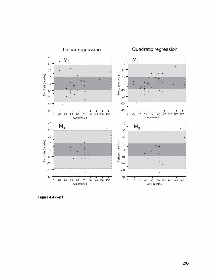
203

Figure 4.4 con’t

-40

-30

-20

-10

0

10

20

30

40

0 20 40 60 80 100 120 140 160 180

Age (months)

-40

-30

-20

-10

0

10

20

30

40

0 20 40 60 80 100 120 140 160 180

Age (months)

-40

-30

-20

-10

0

10

20

30

40

0 20 40 60 80 100 120 140 160 180

Age (months)

-40

-30

-20

-10

0

10

20

30

40

0 20 40 60 80 100 120 140 160 180

Age (months)

M2 M2

M3 M3

Quadratic regressionLinear regression

Res

idua

ls (

mon

ths)

Res

idua

ls (

mon

ths)

Res

idua

ls (

mon

ths)

Res

idua

ls (

mon

ths)

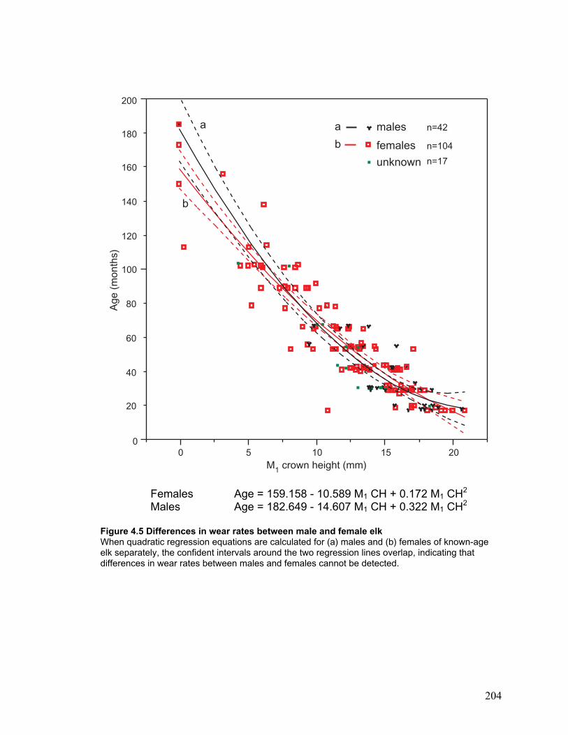
204

Females Age = 159.158 - 10.589 M1 CH + 0.172 M1 CH2

Males Age = 182.649 - 14.607 M1 CH + 0.322 M1 CH2

Figure 4.5 Differences in wear rates between male and female elkWhen quadratic regression equations are calculated for (a) males and (b) females of known-ageelk separately, the confident intervals around the two regression lines overlap, indicating thatdifferences in wear rates between males and females cannot be detected.

males n=42

0

100

200

0 5 10 15 20M1 crown height (mm)

80

60

40

20

180

160

140

120

a

b

females n=104

unknown n=17

Age

(m

onth

s)a

b

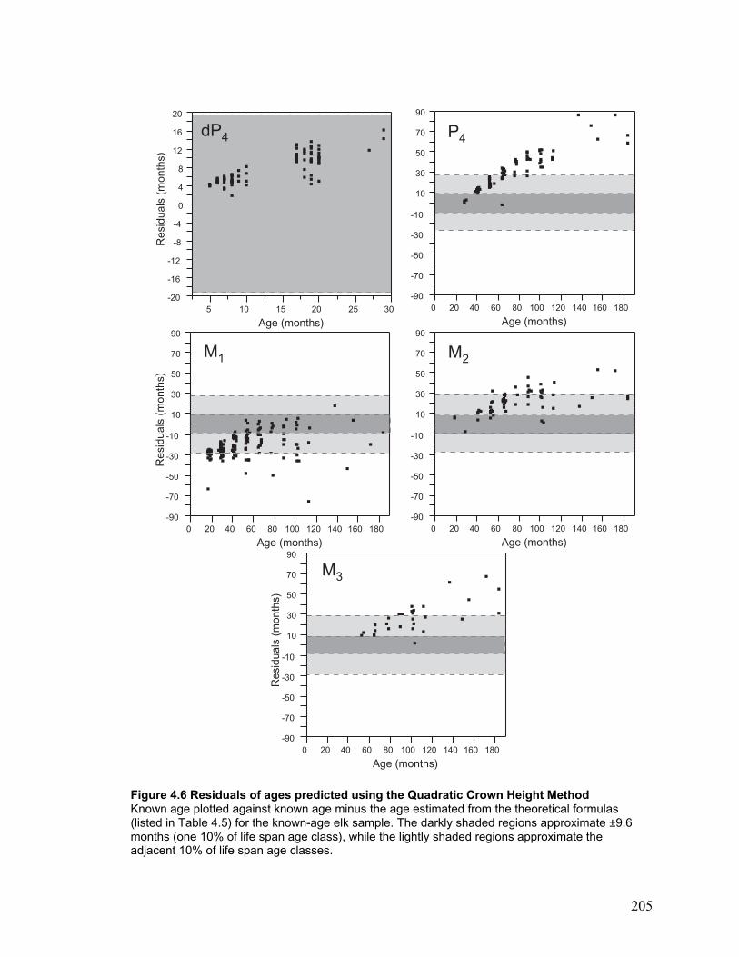
205

Figure 4.6 Residuals of ages predicted using the Quadratic Crown Height MethodKnown age plotted against known age minus the age estimated from the theoretical formulas(listed in Table 4.5) for the known-age elk sample. The darkly shaded regions approximate ±9.6months (one 10% of life span age class), while the lightly shaded regions approximate theadjacent 10% of life span age classes.

-90

-70

-50

-30

-10

10

30

50

70

90

0 20 40 60 80 100 120 140 160 180

Age (months)

P4

-20

-16

-12

-8

-4

0

4

8

12

16

20

5 10 15 20 25 30

Age (months)

dP4

Res

idua

ls (

mon

ths)

-90

-70

-50

-30

-10

10

30

50

70

90

0 20 40 60 80 100 120 140 160 180

Age (months)

-90

-70

-50

-30

-10

10

30

50

70

90

0 20 40 60 80 100 120 140 160 180

Age (months)

M1 M2

Res

idua

ls (

mon

ths)

-90

-70

-50

-30

-10

10

30

50

70

90

0 20 40 60 80 100 120 140 160 180

Age (months)

M3

Res

idua

ls (

mon

ths)

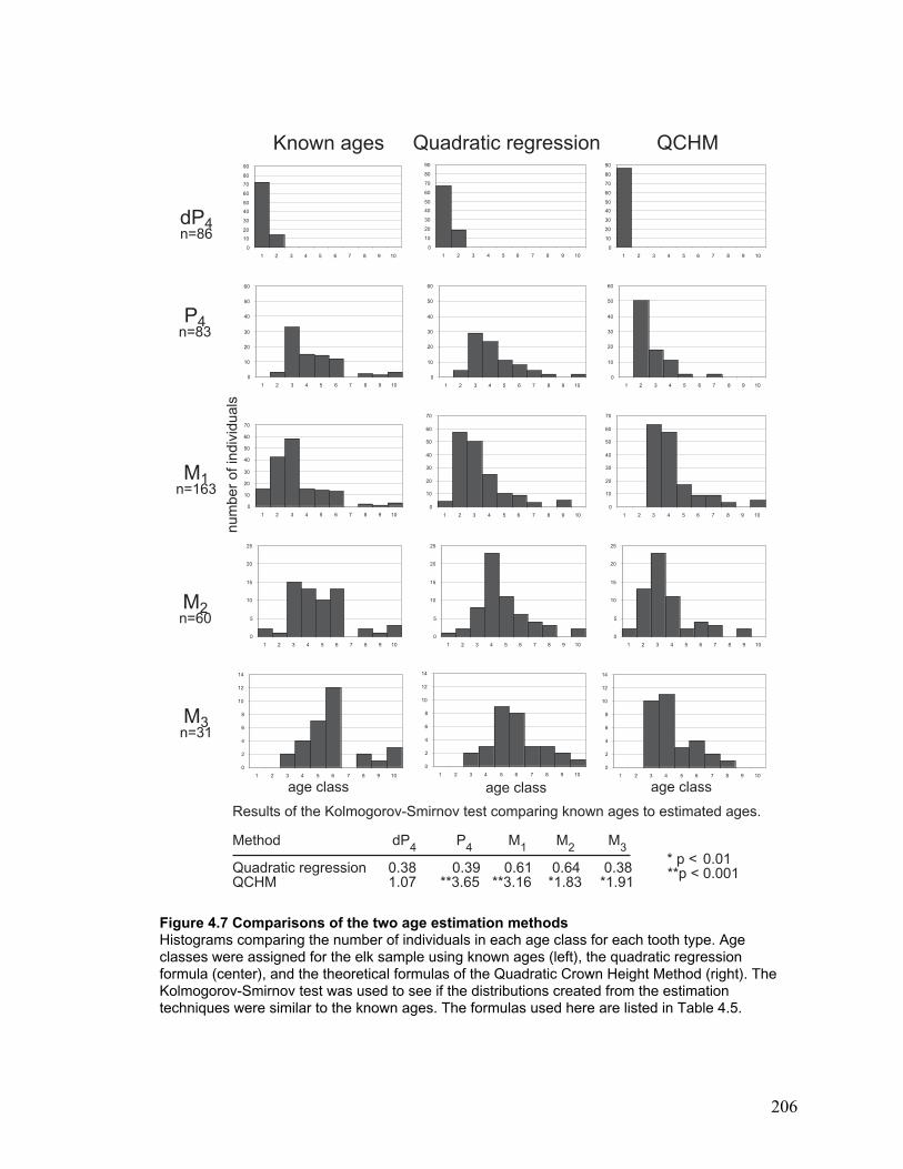
206

Figure 4.7 Comparisons of the two age estimation methodsHistograms comparing the number of individuals in each age class for each tooth type. Ageclasses were assigned for the elk sample using known ages (left), the quadratic regressionformula (center), and the theoretical formulas of the Quadratic Crown Height Method (right). TheKolmogorov-Smirnov test was used to see if the distributions created from the estimationtechniques were similar to the known ages. The formulas used here are listed in Table 4.5.

0

10

20

30

40

50

60

70

80

90

1 2 3 4 5 6 7 8 9 10

0

10

20

30

40

50

60

70

80

90

1 2 3 4 5 6 7 8 9 10

0

10

20

30

40

50

60

70

80

90

1 2 3 4 5 6 7 8 9 10

Known ages QCHM

0

10

20

30

40

50

60

1 2 3 4 5 6 7 8 9 10

0

10

20

30

40

50

60

1 2 3 4 5 6 7 8 9 10

0

10

20

30

40

50

60

1 2 3 4 5 6 7 8 9 10

0

10

20

30

40

50

60

70

1 2 3 4 5 6 7 8 9 10

0

10

20

30

40

50

60

70

1 2 3 4 5 6 7 8 9 10

0

10

20

30

40

50

60

70

1 2 3 4 5 6 7 8 9 10

0

5

10

15

20

25

1 2 3 4 5 6 7 8 9 10

0

5

10

15

20

25

1 2 3 4 5 6 7 8 9 10

0

5

10

15

20

25

1 2 3 4 5 6 7 8 9 10

0

2

4

6

8

10

12

14

1 2 3 4 5 6 7 8 9 10

0

2

4

6

8

10

12

14

1 2 3 4 5 6 7 8 9 100

2

4

6

8

10

12

14

1 2 3 4 5 6 7 8 9 10

Quadratic regression

P4n=83

M1n=163

dP4n=86

M2n=60

M3n=31

age class age class age class

* p < 0.01**p < 0.001

num

ber

of in

divi

dual

s

Results of the Kolmogorov-Smirnov test comparing known ages to estimated ages.

Method dP4 P4 M1 M2 M3

Quadratic regression 0.38 0.39 0.61 0.64 0.38QCHM 1.07 **3.65 **3.16 *1.83 *1.91

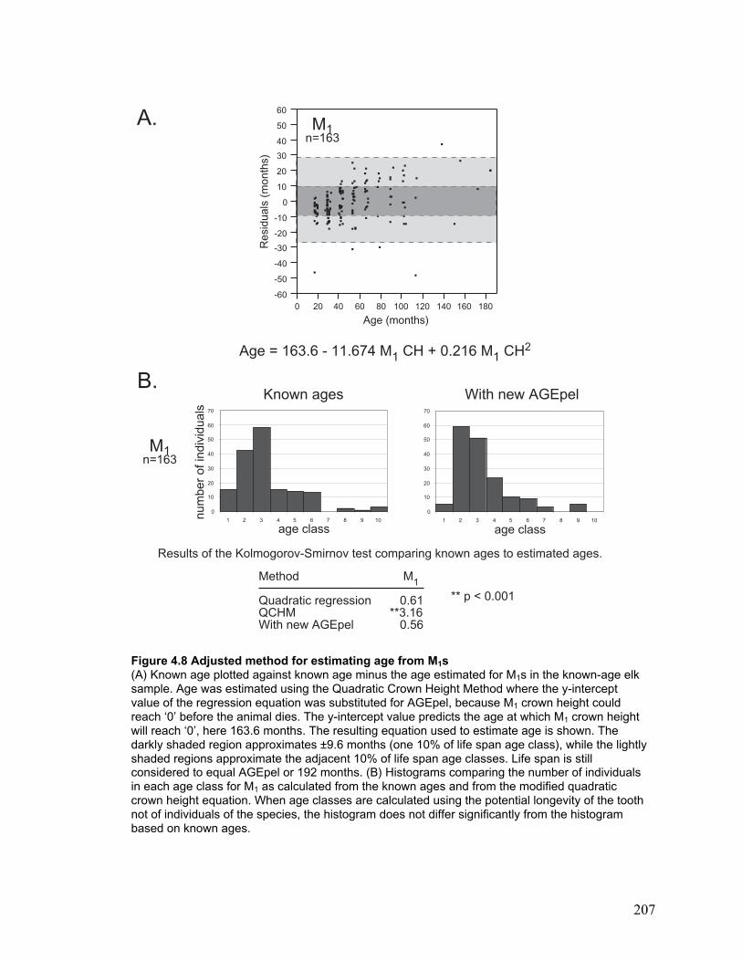
207

Figure 4.8 Adjusted method for estimating age from M1s (A) Known age plotted against known age minus the age estimated for M1s in the known-age elksample. Age was estimated using the Quadratic Crown Height Method where the y-interceptvalue of the regression equation was substituted for AGEpel, because M1 crown height couldreach ‘0’ before the animal dies. The y-intercept value predicts the age at which M1 crown heightwill reach ‘0’, here 163.6 months. The resulting equation used to estimate age is shown. Thedarkly shaded region approximates ±9.6 months (one 10% of life span age class), while the lightlyshaded regions approximate the adjacent 10% of life span age classes. Life span is stillconsidered to equal AGEpel or 192 months. (B) Histograms comparing the number of individualsin each age class for M1 as calculated from the known ages and from the modified quadraticcrown height equation. When age classes are calculated using the potential longevity of the toothnot of individuals of the species, the histogram does not differ significantly from the histogrambased on known ages.

Age = 163.6 - 11.674 M1 CH + 0.216 M1 CH2

A.

B.

-60

-50

-40

-30

-20

-10

0

10

20

30

40

50

60

0 20 40 60 80 100 120 140 160 180

Age (months)

M1n=163

Res

idua

ls (

mon

ths)

M1n=163

num

ber

of in

divi

dual

s

0

10

20

30

40

50

60

70

1 2 3 4 5 6 7 8 9 10

0

10

20

30

40

50

60

70

1 2 3 4 5 6 7 8 9 10

Known ages With new AGEpel

age class age class

Results of the Kolmogorov-Smirnov test comparing known ages to estimated ages.

** p < 0.001

Method M1

Quadratic regression 0.61QCHM **3.16With new AGEpel 0.56

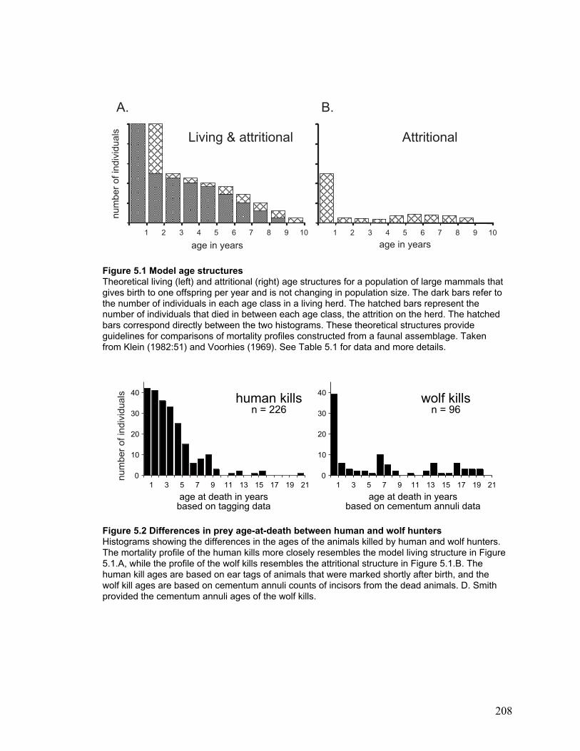
208

Figure 5.1 Model age structuresTheoretical living (left) and attritional (right) age structures for a population of large mammals thatgives birth to one offspring per year and is not changing in population size. The dark bars refer tothe number of individuals in each age class in a living herd. The hatched bars represent thenumber of individuals that died in between each age class, the attrition on the herd. The hatchedbars correspond directly between the two histograms. These theoretical structures provideguidelines for comparisons of mortality profiles constructed from a faunal assemblage. Takenfrom Klein (1982:51) and Voorhies (1969). See Table 5.1 for data and more details.

Figure 5.2 Differences in prey age-at-death between human and wolf huntersHistograms showing the differences in the ages of the animals killed by human and wolf hunters.The mortality profile of the human kills more closely resembles the model living structure in Figure5.1.A, while the profile of the wolf kills resembles the attritional structure in Figure 5.1.B. Thehuman kill ages are based on ear tags of animals that were marked shortly after birth, and thewolf kill ages are based on cementum annuli counts of incisors from the dead animals. D. Smithprovided the cementum annuli ages of the wolf kills.

age in years

AttritionalLiving & attritional

age in years

1 2 3 4 5 6 7 8 9 10 1 2 3 4 5 6 7 8 9 10

num

ber

of in

divi

dual

sA. B.

0

10

20

30

40

1 3 5 7 9 11 13 15 17 19 21

human killsn = 226

wolf killsn = 96

age at death in yearsbased on tagging data

age at death in yearsbased on cementum annuli data

0

10

20

30

40

1 3 5 7 9 11 13 15 17 19 21

num

ber

of in

divi

dual

s

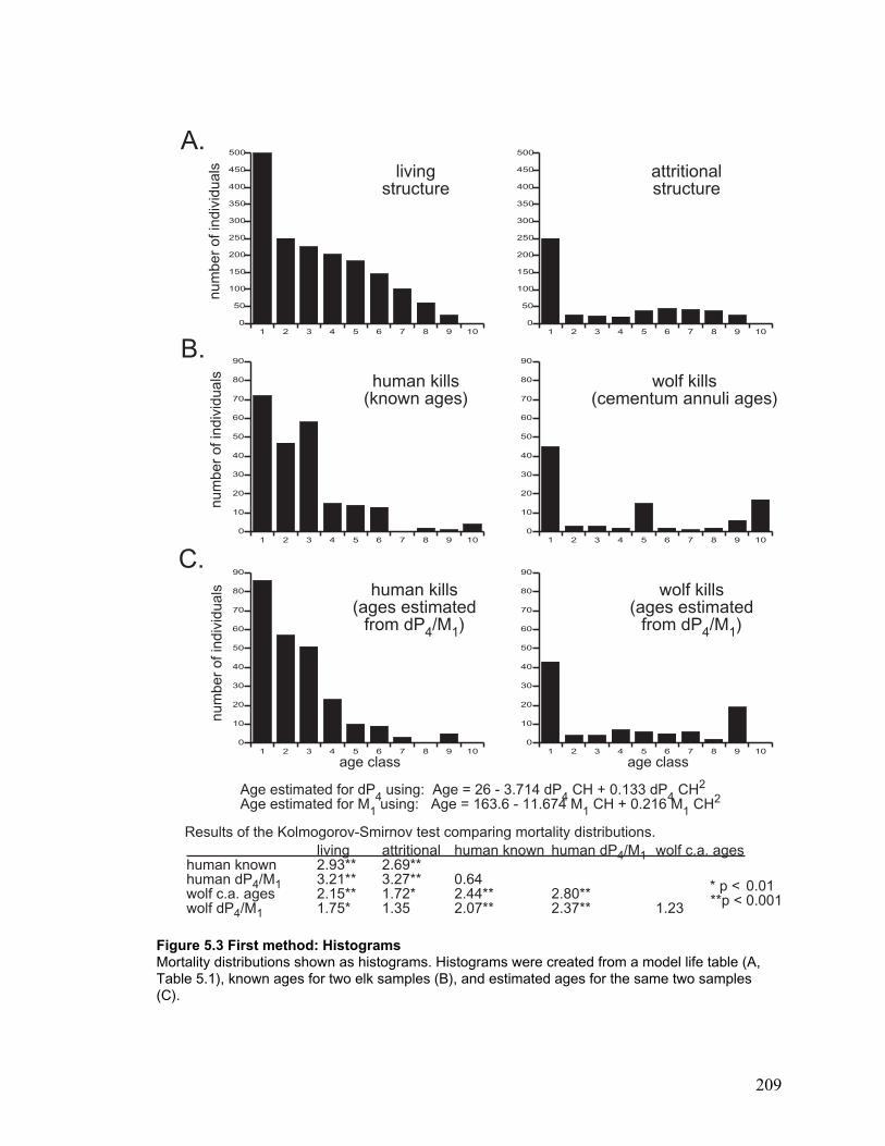
209

Figure 5.3 First method: HistogramsMortality distributions shown as histograms. Histograms were created from a model life table (A,Table 5.1), known ages for two elk samples (B), and estimated ages for the same two samples(C).

1 2 3 4 5 6 7 8 9 100

50

100

150

200

250

300

350

400

450

500

1 2 3 4 5 6 7 8 9 100

50

100

150

200

250

300

350

400

450

500

num

ber

of in

divi

dual

s livingstructure

attritionalstructure

1 2 3 4 5 6 7 8 9 100

10

20

30

40

50

60

70

80

90

1 2 3 4 5 6 7 8 9 100

10

20

30

40

50

60

70

80

90

num

ber

of in

divi

dual

s human kills(known ages)

wolf kills(cementum annuli ages)

1 2 3 4 5 6 7 8 9 100

10

20

30

40

50

60

70

80

90

1 2 3 4 5 6 7 8 9 100

10

20

30

40

50

60

70

80

90

age class

num

ber

of in

divi

dual

s

age class

human kills(ages estimated

from dP4/M1)

wolf kills(ages estimated

from dP4/M1)

Age estimated for dP4 using: Age = 26 - 3.714 dP4 CH + 0.133 dP4 CH2

Age estimated for M1 using: Age = 163.6 - 11.674 M1 CH + 0.216 M1 CH2

A.

B.

C.

Results of the Kolmogorov-Smirnov test comparing mortality distributions.

* p < 0.01**p < 0.001

living attritional human known human dP4/M1 wolf c.a. ageshuman known 2.93** 2.69**human dP4/M1 3.21** 3.27** 0.64wolf c.a. ages 2.15** 1.72* 2.44** 2.80**wolf dP4/M1 1.75* 1.35 2.07** 2.37** 1.23

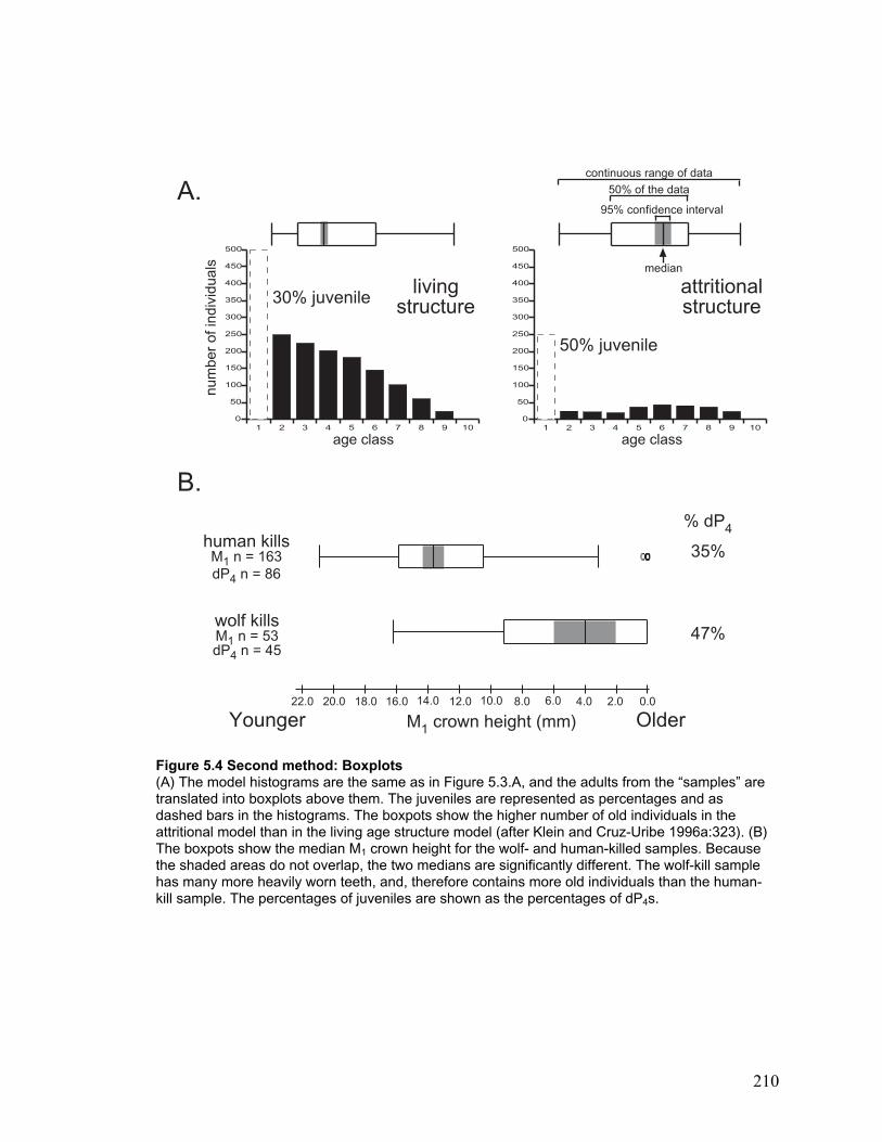
210

Figure 5.4 Second method: Boxplots(A) The model histograms are the same as in Figure 5.3.A, and the adults from the “samples” aretranslated into boxplots above them. The juveniles are represented as percentages and asdashed bars in the histograms. The boxpots show the higher number of old individuals in theattritional model than in the living age structure model (after Klein and Cruz-Uribe 1996a:323). (B)The boxpots show the median M1 crown height for the wolf- and human-killed samples. Becausethe shaded areas do not overlap, the two medians are significantly different. The wolf-kill samplehas many more heavily worn teeth, and, therefore contains more old individuals than the human-kill sample. The percentages of juveniles are shown as the percentages of dP4s.

1 2 3 4 5 6 7 8 9 100

50

100

150

200

250

300

350

400

450

500

1 2 3 4 5 6 7 8 9 100

50

100

150

200

250

300

350

400

450

500

num

ber

of in

divi

dual

s

livingstructure

attritionalstructure

A.

B.

30% juvenile

50% juvenile

human killsM1 n = 163dP4 n = 86

wolf killsM1 n = 53dP4 n = 45

age class age class

% dP4

35%

47%

M1 crown height (mm) OlderYounger22.0 20.0 18.0 16.0 14.0 12.0 10.0 8.0 6.0 4.0 2.0 0.0

median

continuous range of data

95% confidence interval

50% of the data

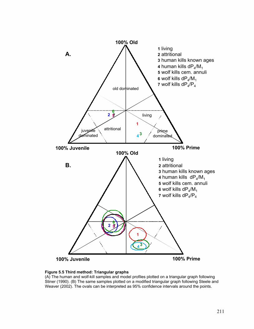
211

Figure 5.5 Third method: Triangular graphs(A) The human and wolf-kill samples and model profiles plotted on a triangular graph followingStiner (1990). (B) The same samples plotted on a modified triangular graph following Steele andWeaver (2002). The ovals can be interpreted as 95% confidence intervals around the points.

1 living2 attritional3 human kills known ages4 human kills dP4/M1

5 wolf kills cem. annuli6 wolf kills dP4/M1

7 wolf kills dP4/P4

A.

B.

100% Old

100% Juvenile 100% Prime

1 living2 attritional3 human kills known ages4 human kills dP4/M15 wolf kills cem. annuli6 wolf kills dP4/M17 wolf kills dP4/P4

old dominated

juveniledominated

primedominated

living

attritional

100% Old

100% Juvenile 100% Prime

1

2

34

567

1

2

34

567

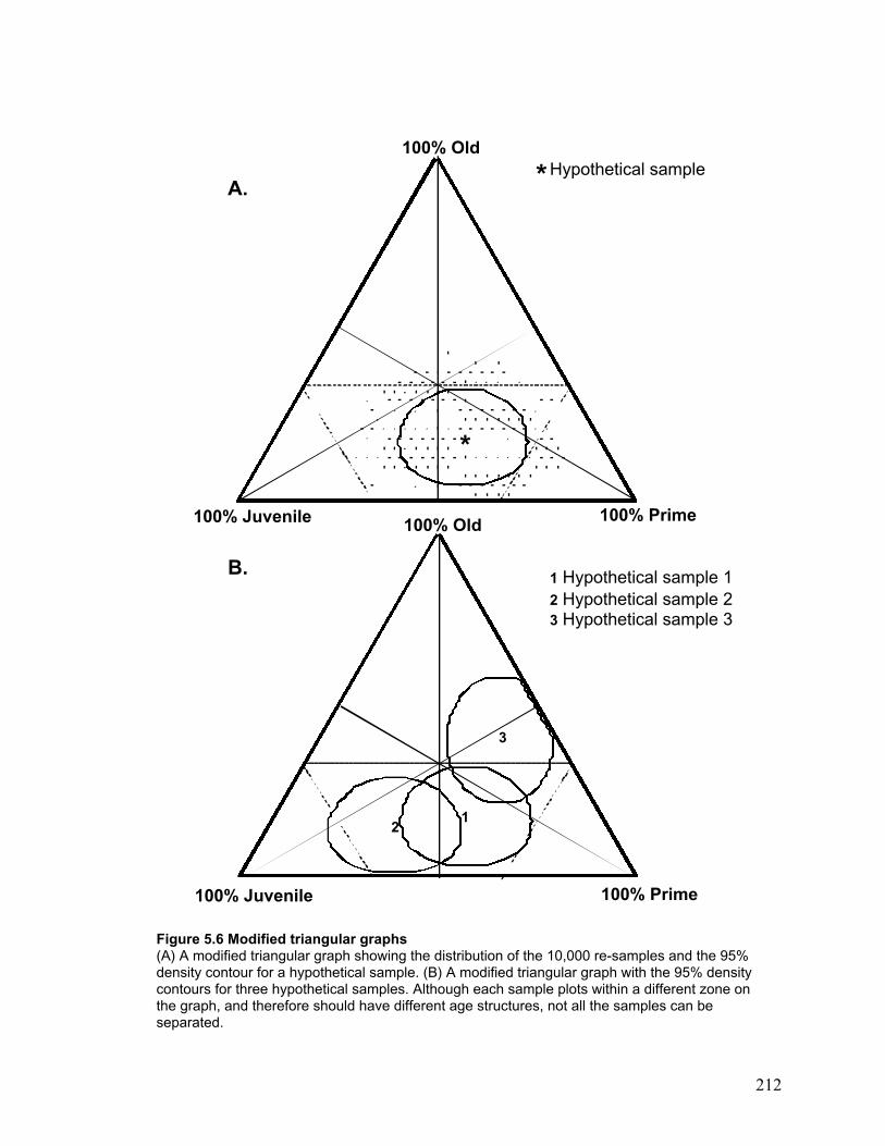
212

Figure 5.6 Modified triangular graphs(A) A modified triangular graph showing the distribution of the 10,000 re-samples and the 95%density contour for a hypothetical sample. (B) A modified triangular graph with the 95% densitycontours for three hypothetical samples. Although each sample plots within a different zone onthe graph, and therefore should have different age structures, not all the samples can beseparated.

B.

100% Old

100% Juvenile 100% Prime

1 Hypothetical sample 12 Hypothetical sample 23 Hypothetical sample 3

A.

100% Old

100% Juvenile 100% Prime

Hypothetical sample

*

*

3

12

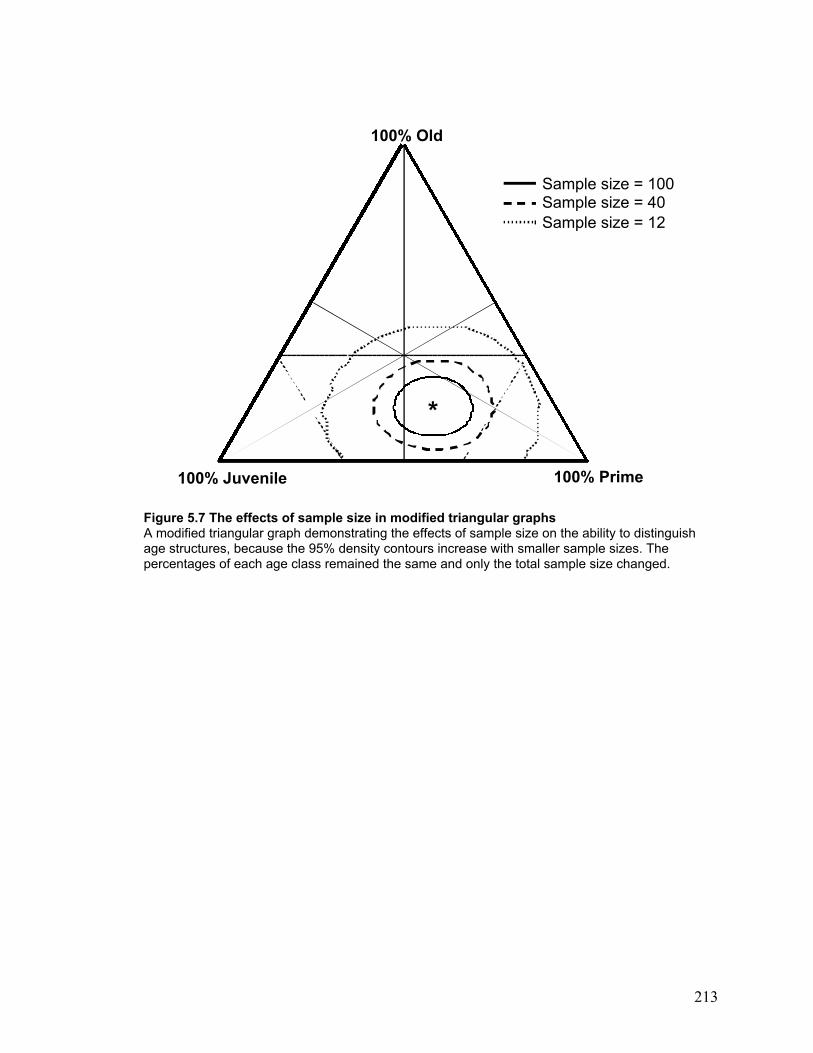
213

Figure 5.7 The effects of sample size in modified triangular graphsA modified triangular graph demonstrating the effects of sample size on the ability to distinguishage structures, because the 95% density contours increase with smaller sample sizes. Thepercentages of each age class remained the same and only the total sample size changed.

100% Old

100% Juvenile 100% Prime

*

Sample size = 100Sample size = 40Sample size = 12

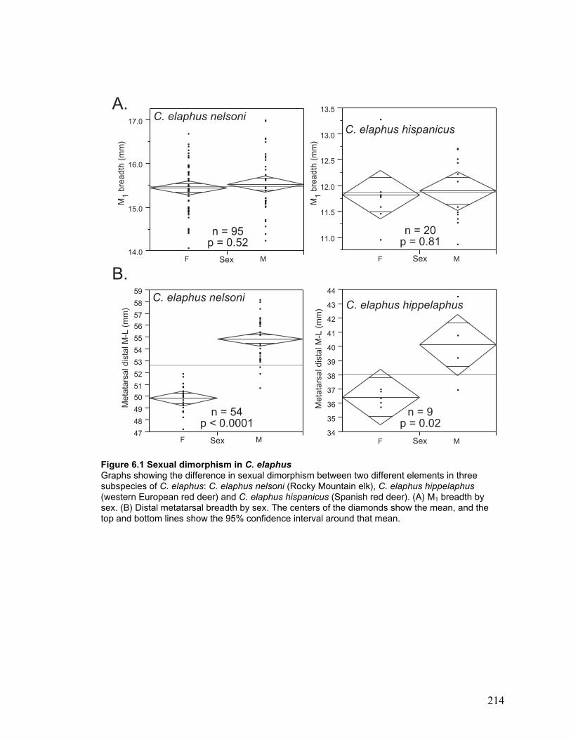
214

Figure 6.1 Sexual dimorphism in C. elaphusGraphs showing the difference in sexual dimorphism between two different elements in threesubspecies of C. elaphus: C. elaphus nelsoni (Rocky Mountain elk), C. elaphus hippelaphus(western European red deer) and C. elaphus hispanicus (Spanish red deer). (A) M1 breadth bysex. (B) Distal metatarsal breadth by sex. The centers of the diamonds show the mean, and thetop and bottom lines show the 95% confidence interval around that mean.

14.0

15.0

16.0

17.0M

1 bre

adth

(m

m)

M1 b

read

th (

mm

)

11.0

11.5

12.0

12.5

13.0

13.5C. elaphus nelsoni

SexF M SexF M

C. elaphus hispanicus

n = 95p = 0.52

n = 20p = 0.81

Sex34

35

36

37

38

39

40

41

42

43

44

F M

Met

atar

sal d

ista

l M-L

(m

m)

Sex47

48

49

50

51

52

53

54

55

56

57

58

59

F M

Met

atar

sal d

ista

l M-L

(m

m)

n = 54p < 0.0001

n = 9p = 0.02

C. elaphus nelsoniC. elaphus hippelaphus

A.

B.

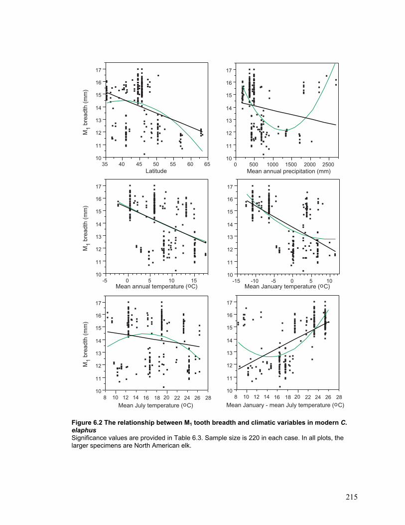
215

Figure 6.2 The relationship between M1 tooth breadth and climatic variables in modern C.elaphusSignificance values are provided in Table 6.3. Sample size is 220 in each case. In all plots, thelarger specimens are North American elk.

10 208 12 14 16 18 22 24 26 2810 208 12 14 16 18 22 24 26 28

Mean January temperature ( C)oMean annual temperature ( C)o

10

11

12

13

14

15

16

17

35 40 45 50 55 60 65Latitude

Mean July temperature ( C)o

Mean annual precipitation (mm)

M1 b

read

th (

mm

)M

1 bre

adth

(m

m)

M1 b

read

th (

mm

)

Mean January - mean July temperature ( C)o

10

11

12

13

14

15

16

17

0 500 1000 1500 2000 2500

10

11

12

13

14

15

16

17

10

11

12

13

14

15

16

17

10

11

12

13

14

15

16

17

-15 -10 -5 0 5 1010

11

12

13

14

15

16

17

-5 0 5 10 15

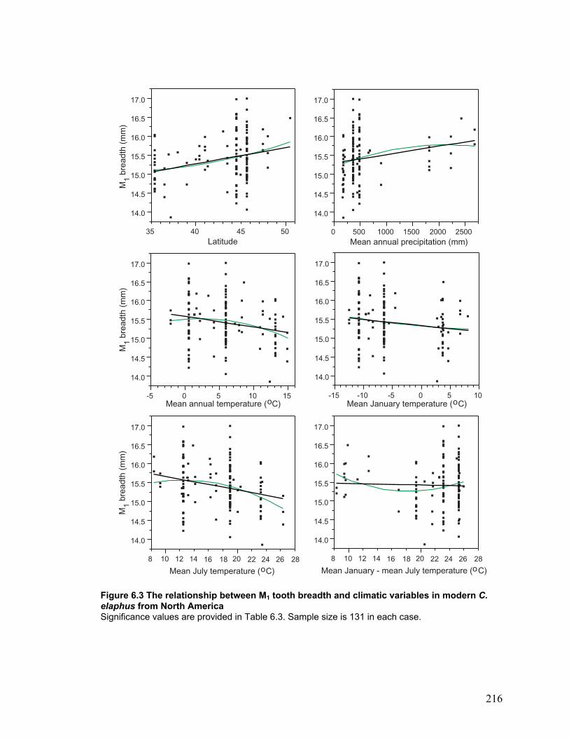
216

Figure 6.3 The relationship between M1 tooth breadth and climatic variables in modern C.elaphus from North AmericaSignificance values are provided in Table 6.3. Sample size is 131 in each case.

14.0

14.5

15.0

15.5

16.0

16.5

17.0

-15 -10 -5 0 5 10

14.0

14.5

15.0

15.5

16.0

16.5

17.0

-5 0 5 10 15

M1 b

read

th (

mm

)M

1 bre

adth

(m

m)

14.0

14.5

15.0

15.5

16.0

16.5

17.0

40 50

14.0

14.5

15.0

15.5

16.0

16.5

17.0

0 500 1000 1500 2000 2500

14.0

14.5

15.0

15.5

16.0

16.5

17.0

14.0

14.5

15.0

15.5

16.0

16.5

17.0

10 20

4535

M1 b

read

th (

mm

)

8 12 14 16 18 22 24 26 2810 208 12 14 16 18 22 24 26 28

Mean January temperature ( C)Mean annual temperature ( C)

Latitude

Mean July temperature ( C)

Mean annual precipitation (mm)

Mean January - mean July temperature ( C)

o o

oo

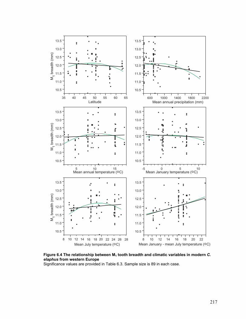
217

Figure 6.4 The relationship between M1 tooth breadth and climatic variables in modern C.elaphus from western EuropeSignificance values are provided in Table 6.3. Sample size is 89 in each case.

10 208 12 14 16 18 22 24 26 28

Mean July temperature ( C)o

10.5

11.0

11.5

12.0

12.5

13.0

13.5

35 40 45 50 55 60 65Latitude

10.5

11.0

11.5

12.0

12.5

13.0

13.5

600 1000 1400 1800 2200Mean annual precipitation (mm)

10.5

11.0

11.5

12.0

12.5

13.0

13.5

10

10.5

11.0

11.5

12.0

12.5

13.0

13.5

10.5

11.0

11.5

12.0

12.5

13.0

13.5

10.5

11.0

11.5

12.0

12.5

13.0

13.5

8 10 12 14 16 18 20 22

M1 b

read

th (

mm

)M

1 bre

adth

(m

m)

M1 b

read

th (

mm

)

Mean January temperature ( C)o

Mean January - mean July temperature ( C)o

0 10-5 55 15Mean annual temperature ( C)o

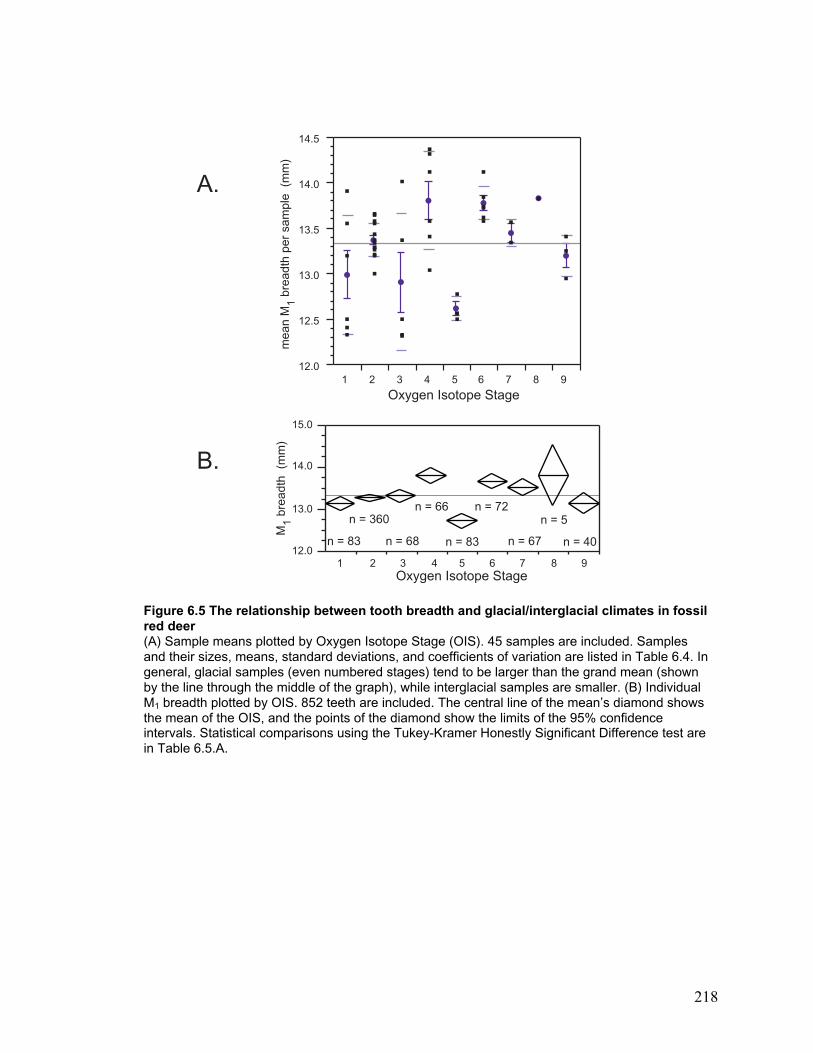
218

Figure 6.5 The relationship between tooth breadth and glacial/interglacial climates in fossilred deer(A) Sample means plotted by Oxygen Isotope Stage (OIS). 45 samples are included. Samplesand their sizes, means, standard deviations, and coefficients of variation are listed in Table 6.4. Ingeneral, glacial samples (even numbered stages) tend to be larger than the grand mean (shownby the line through the middle of the graph), while interglacial samples are smaller. (B) IndividualM1 breadth plotted by OIS. 852 teeth are included. The central line of the mean’s diamond showsthe mean of the OIS, and the points of the diamond show the limits of the 95% confidenceintervals. Statistical comparisons using the Tukey-Kramer Honestly Significant Difference test arein Table 6.5.A.

Oxygen Isotope Stage

mea

n M

1 bre

adth

per

sam

ple

(m

m)

A.

12.0

12.5

13.0

13.5

14.0

14.5

1 2 3 4 5 6 7 8 9

B.

Oxygen Isotope Stage

M1 b

read

th (

mm

)

1 2 3 4 5 6 7 8 912.0

13.0

14.0

15.0

n = 83

n = 360

n = 68

n = 66

n = 83

n = 72

n = 67

n = 5

n = 40

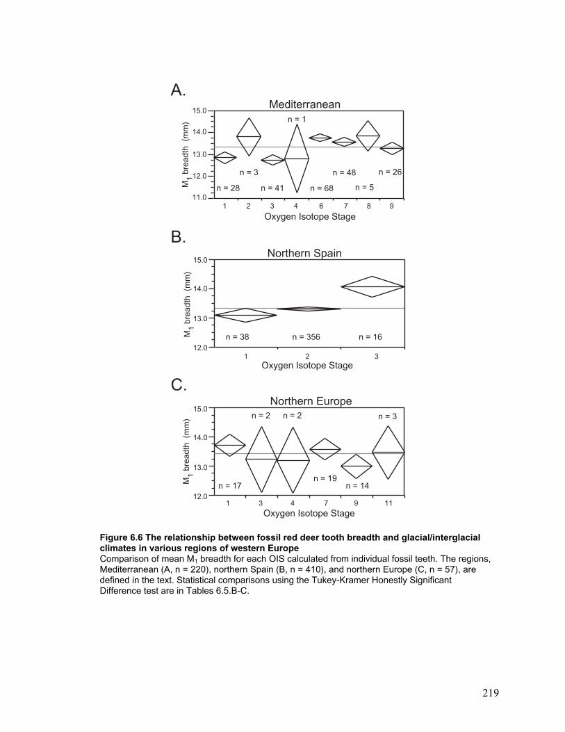
219

Figure 6.6 The relationship between fossil red deer tooth breadth and glacial/interglacialclimates in various regions of western EuropeComparison of mean M1 breadth for each OIS calculated from individual fossil teeth. The regions,Mediterranean (A, n = 220), northern Spain (B, n = 410), and northern Europe (C, n = 57), aredefined in the text. Statistical comparisons using the Tukey-Kramer Honestly SignificantDifference test are in Tables 6.5.B-C.

Oxygen Isotope Stage

M1 b

read

th (

mm

)

Mediterranean

1 2 3 4 6 7 8 9

12.0

13.0

14.0

15.0

11.0n = 28

n = 3

n = 41

n = 1

n = 68

n = 48

n = 5

n = 26

A.

Oxygen Isotope Stage

M1 b

read

th (

mm

)

Northern Spain

112.0

13.0

14.0

15.0

2 3

n = 38 n = 356 n = 16

B.

Oxygen Isotope Stage

M1 b

read

th (

mm

)

Northern Europe

12.0

13.0

14.0

15.0

1 3 4 7 9 11

n = 17

n = 2 n = 2

n = 19n = 14

n = 3

C.

220

Figure 6.7 Variation in fossil red deer M1 breadth during different Oxygen Isotope StagesComparisons of tooth breadth between regions during individual Oxygen Isotope Stages. Theregions, Mediterranean, northern Spain, and northern Europe, are defined in the text.

M1 b

read

th (

mm

)

Oxygen Isotope Stage 1

M1 b

read

th (

mm

)

Mediterraneann = 26

NorthernEuropen = 14

Oxygen Isotope Stage 9

10.0

11.0

12.0

13.0

14.0

15.0

16.0

p = 0.3874

M1 b

read

th (

mm

)

M1 b

read

th (

mm

)

Mediterraneann = 28

NorthernEuropen = 17

NorthernSpainn = 38

11.0

12.0

13.0

14.0

15.0Oxygen Isotope Stage 3

Mediterraneann = 41

NorthernSpainn = 16

11.0

12.0

13.0

14.0

15.0

p < 0.0001

Mediterraneann = 48

NorthernEuropen = 19

Oxygen Isotope Stage 7

12.0

13.0

14.0

15.0

16.0

p = 0.8879

Med. N. EuropeN. Europe **N. Spain ns **

** significantly different with bothstudent’s t-test and Tukey-Kramer HSD

221

Figure 6.8 The relationship between distal metatarsal breadth and climatic variables inmodern C. elaphus from North AmericaRegression lines are calculated separately for males (n = 50) and females (n = 35); in all casesthe males are the upper line. Climatic data are in Table 6.2, and summary statistics are in Table6.6.

Latitude Mean annual precipitation (mm)

dist

al m

etat

arsa

l bre

adth

(m

m)

44

46

48

50

52

54

56

58

60

200 300 400 500 600 70044

46

48

50

52

54

56

58

60

34 36 38 40 42 44 46 48

r = 0.422r = 0.392

r = 0.372

r = 0.342

44

46

48

50

52

54

56

58

60

-5 0 5 10 15Mean annual temperature ( C)o

dist

al m

etat

arsa

l bre

adth

(m

m)

44

46

48

50

52

54

56

58

60

-15 -10 -5 0 5 10Mean January temperature ( C)o

r = 0.272

r = 0.392

r = 0.322

r = 0.402

C. elaphus nannodesC. elaphus nelsoniC. elaphus roosevelti

44

46

48

50

52

54

56

58

60

5 10 15 20 2544

46

48

50

52

54

56

58

60

5 10 15 20 25

dist

al m

etat

arsa

l bre

adth

(m

m)

Mean July temperature ( C) Mean January - mean July temperature ( C)o o

r = 0.402

r = 0.382

r = 0.032

r = 0.242

222

Figure 6.9 Variation in fossil red deer distal metacarpal breadth during different OxygenIsotope StagesThe central line of the means diamond shows the mean of the OIS, and the points of the diamondshow the limits of the 95% confidence intervals. The samples total 161 individuals.

Mediterranean n = 28Northern Spain n = 133

34

36

38

40

42

44

46

48

50

52

1 2 3 4 6

dist

al m

etac

arpa

l bre

adth

(m

m)

Oxygen Isotope Stage

n = 7 n = 101 n = 23 n = 9 n = 21

OIS 1 2 3 42 **3 ** **4 ** ns ns6 ** ns ** ns

** significantly different with Tukey-Kramer HSD

223

Figure 7.1 First analysis: Histograms of individual samplesSamples with a combined total of measurable dP4s and M1s of greater than 25. Age classes arebased on 10% of life span (19.2 months for C. elaphus), but no individuals plotted in the oldestage class. Kolmogorov-Smirnov results are listed in Table 7.2.

El Castillo (Mag)n = 97

Combe-Grenal 50n = 38

Combe-Grenal 52n = 27

El Juyo 4n = 43

El Juyo 6n = 100

El Juyo 8n = 26

Gabasa en = 31

Gabasa fn = 24

Lazaret En = 26

Urtiaga Cn = 24

Urtiaga Dn = 48

Urtiaga Fn = 28

1 2 3 4 5 6 7 8 9 0

2

4

6

8

10

12

14

1 2 3 4 5 6 7 8 9 0

1

2

3

4

5

6

7

8

9

1 2 3 4 5 6 7 8 9

1 2 3 4 5 6 7 8 9 0

10

20

30

40

50

60

1 2 3 4 5 6 7 8 9 0

2

4

6

8

10

12

14

16

18

1 2 3 4 5 6 7 8 9

1 2 3 4 5 6 7 8 9 0

5

10

15

20

25

1 2 3 4 5 6 7 8 9 0

1

2

3

4

5

6

7

1 2 3 4 5 6 7 8 9

1 2 3 4 5 6 7 8 9 0

5

10

15

20

25

30

35

1 2 3 4 5 6 7 8 9 0

2

4

6

8

10

12

14

1 2 3 4 5 6 7 8 9

0

10

20

30

40

50

60

0

5

10

15

20

25

30

0

5

10

15

20

25

0

2

4

6

8

10

12

num

ber

of in

divi

dual

snu

mbe

r of

indi

vidu

als

num

ber

of in

divi

dual

snu

mbe

r of

indi

vidu

als

age class

Recent humansn = 245

Wolvesn = 96

1 2 3 4 5 6 7 8 9 05

101520253035404550

1 2 3 4 5 6 7 8 90

102030405060708090100

num

ber

of in

divi

dual

s

age class age class

224

Figure 7.2 First analysis: Boxplots of individual samplesSamples have a combined total of dP4 and M1 of greater than 25 and are standardized by themean unworn crown height of that sample. The darkly shaded area for each sampleapproximates the 95% confidence intervals around each median, and if these regions for twosamples do not overlap, they can be considered significantly different. The central lightly shadedarea approximates the region for prime adult animals.

0.000.250.500.751.001.25M1 crown height

mean unworn crown heightOlderYounger

Wolvesn = 53

Urtiaga Fn = 28

Urtiaga Dn = 33

Urtiaga Cn = 24

Lazaret En = 22

Recent humansn = 164

Gabasa en = 17

El Juyo 8n = 26

El Juyo 6n = 97

Combe-Grenal 52n = 27

Combe-Grenal 50n = 38

El Castillo (Mag)n = 61

Gabasa fn = 7

El Juyo 4n = 32

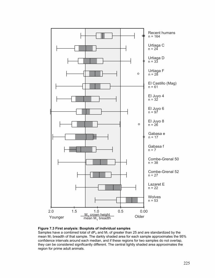
225

Figure 7.3 First analysis: Boxplots of individual samplesSamples have a combined total of dP4 and M1 of greater than 25 and are standardized by themean M1 breadth of that sample. The darkly shaded area for each sample approximates the 95%confidence intervals around each median, and if these regions for two samples do not overlap,they can be considered significantly different. The central lightly shaded area approximates theregion for prime adult animals.

0.000.51.01.52.0OlderYounger

Wolvesn = 53

Urtiaga Fn = 28

Urtiaga Dn = 33

Urtiaga Cn = 24

Lazaret En = 22

Recent humansn = 164

Gabasa en = 17

El Juyo 8n = 26

El Juyo 6n = 97

Combe-Grenal 52n = 27

Combe-Grenal 50n = 38

El Castillo (Mag)n = 61

Gabasa fn = 7

El Juyo 4n = 32

M1 crown heightmean M1 breadth

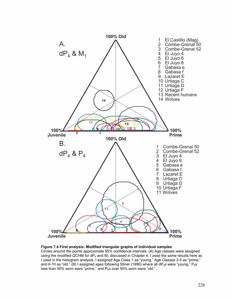
226

Figure 7.4 First analysis: Modified triangular graphs of individual samplesCircles around the points approximate 95% confidence intervals. (A) Age classes were assignedusing the modified QCHM for dP4 and M1 discussed in Chapter 4. I used the same results here asI used in the histogram analysis. I assigned Age Class 1 as “young,” Age Classes 2-5 as “prime,”and 6-10 as “old.” (B) I assigned ages following Stiner (1990) where all dP4s were “young,” P4sless than 50% worn were “prime,” and P4s over 50% worn were “old.”

1 El Castillo (Mag)2 Combe-Grenal 503 Combe-Grenal 524 El Juyo 45 El Juyo 66 El Juyo 87 Gabasa e8 Gabasa f9 Lazaret E10 Urtiaga C11 Urtiaga D12 Urtiaga F13 Recent humans14 Wolves

100% Old

100%Juvenile

100%Prime

100% Old

100%Juvenile

100%Prime

1 Combe-Grenal 502 Combe-Grenal 523 El Juyo 44 El Juyo 65 Gabasa e6 Gabasa f7 Lazaret E8 Urtiaga C9 Urtiaga D10 Urtiaga F11 Wolves

4

6

7

9

11

123

58

10

A.

B.

dP4 & M1

dP4 & P4

8

11

14

1 2 34

567

9

10 1213

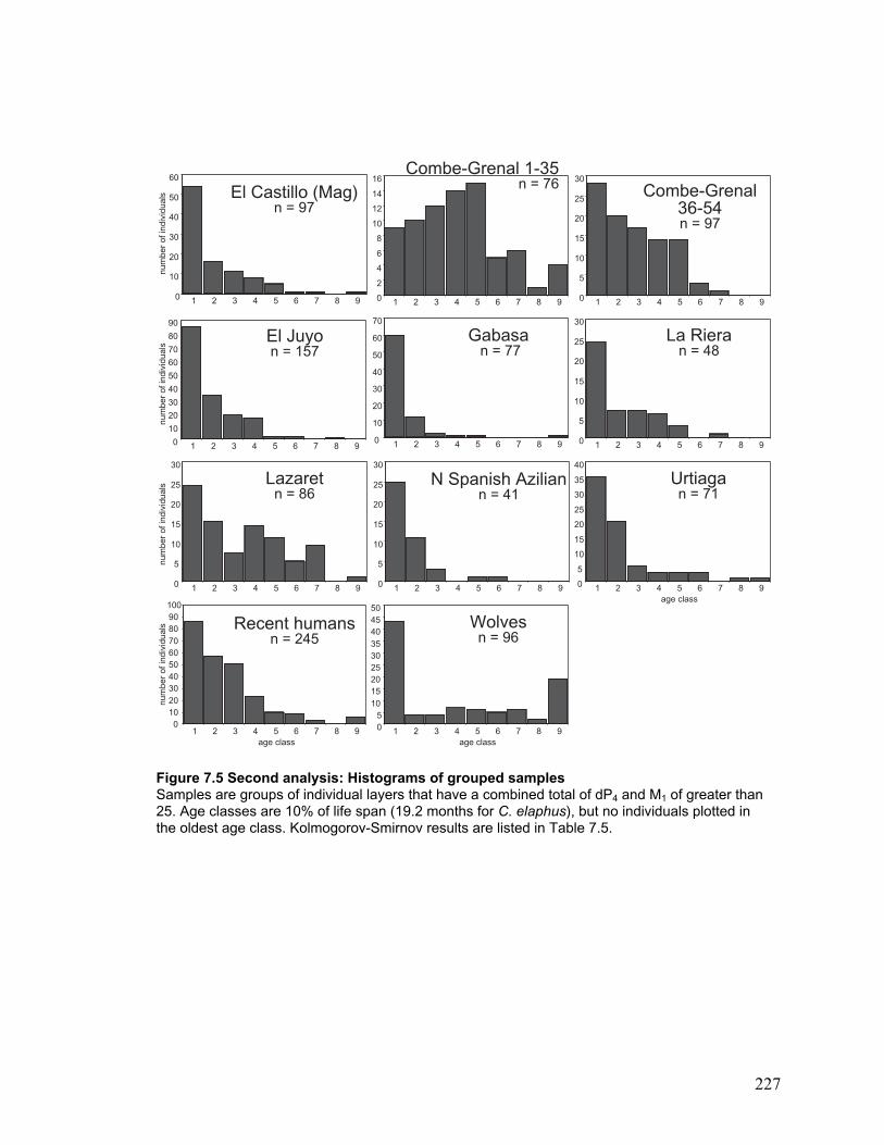
227

Figure 7.5 Second analysis: Histograms of grouped samplesSamples are groups of individual layers that have a combined total of dP4 and M1 of greater than25. Age classes are 10% of life span (19.2 months for C. elaphus), but no individuals plotted inthe oldest age class. Kolmogorov-Smirnov results are listed in Table 7.5.

0

10

20

30

40

50

60

1 2 3 4 5 6 7 8 9

El Castillo (Mag)n = 97

0

2

4

6

8

10

12

14

16

1 2 3 4 5 6 7 8 9

Combe-Grenal 1-35n = 76

0

5

10

15

20

25

30

1 2 3 4 5 6 7 8 9

Combe-Grenal36-54n = 97

0

10

20

30

40

50

60

70

80

90

1 2 3 4 5 6 7 8 9

El Juyon = 157

0

10

20

30

40

50

60

70

1 2 3 4 5 6 7 8 9

Gabasa n = 77

0

5

10

15

20

25

30

1 2 3 4 5 6 7 8 9

Lazaretn = 86

0

5

10

15

20

25

30

1 2 3 4 5 6 7 8 9

N Spanish Aziliann = 41

Recent humansn = 245

Wolvesn = 96

1 2 3 4 5 6 7 8 9 05

101520253035404550

1 2 3 4 5 6 7 8 90

102030405060708090100

num

ber

of in

divi

dual

s

age class age class

num

ber

of in

divi

dual

snu

mbe

r of

indi

vidu

als

num

ber

of in

divi

dual

s

0

5

10

15

20

25

30

1 2 3 4 5 6 7 8 9

La Rieran = 48

0

5

10

15

20

25

30

35

40

1 2 3 4 5 6 7 8 9

Urtiagan = 71

age class

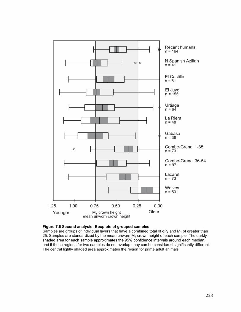
228

Figure 7.6 Second analysis: Boxplots of grouped samplesSamples are groups of individual layers that have a combined total of dP4 and M1 of greater than25. Samples are standardized by the mean unworn M1 crown height of each sample. The darklyshaded area for each sample approximates the 95% confidence intervals around each median,and if these regions for two samples do not overlap, they can be considered significantly different.The central lightly shaded area approximates the region for prime adult animals.

M1 crown heightmean unworn crown height

OlderYounger

El Juyon = 155

El Castillon = 61

N Spanish Aziliann = 41

Recent humansn = 164

Combe-Grenal 36-54n = 97

Combe-Grenal 1-35n = 73

Gabasan = 38

Wolvesn = 53

Lazaretn = 73

La Rieran = 48

Urtiagan = 64

0.000.250.500.751.001.25

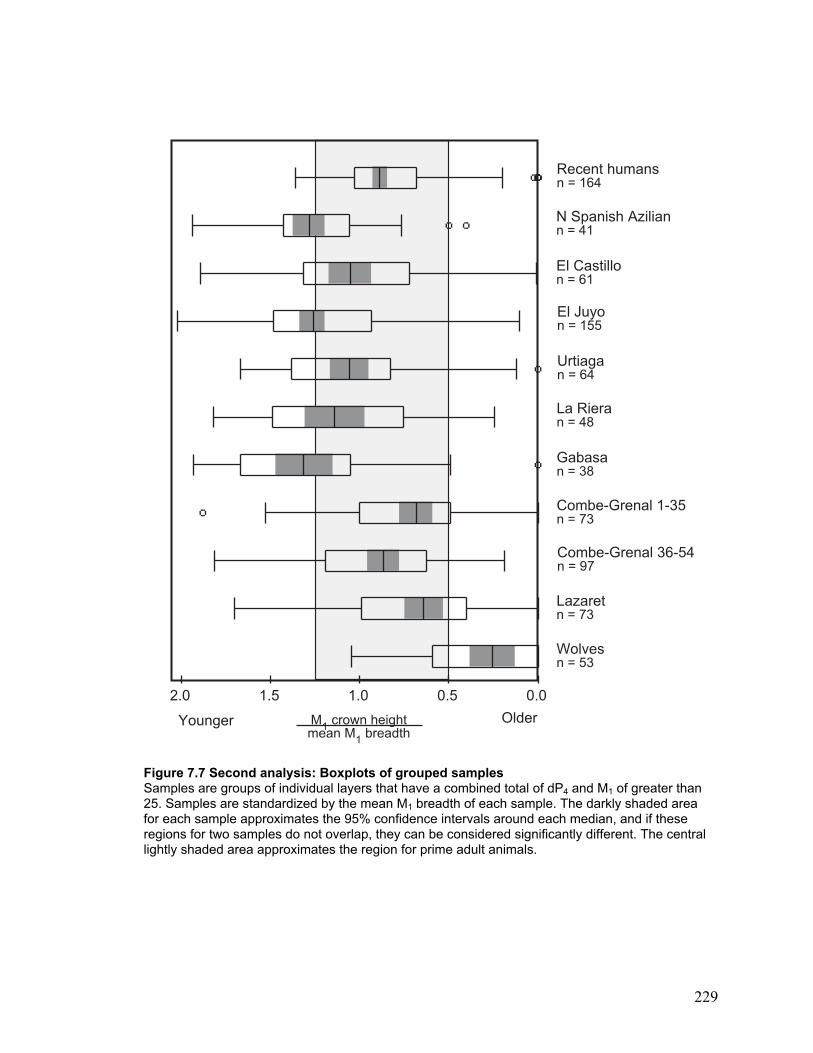
229

Figure 7.7 Second analysis: Boxplots of grouped samplesSamples are groups of individual layers that have a combined total of dP4 and M1 of greater than25. Samples are standardized by the mean M1 breadth of each sample. The darkly shaded areafor each sample approximates the 95% confidence intervals around each median, and if theseregions for two samples do not overlap, they can be considered significantly different. The centrallightly shaded area approximates the region for prime adult animals.

M1 crown heightmean M1 breadth

OlderYounger

El Juyon = 155

El Castillon = 61

N Spanish Aziliann = 41

Recent humansn = 164

Combe-Grenal 36-54n = 97

Combe-Grenal 1-35n = 73

Gabasan = 38

Wolvesn = 53

Lazaretn = 73

La Rieran = 48

Urtiagan = 64

0.00.51.01.52.0

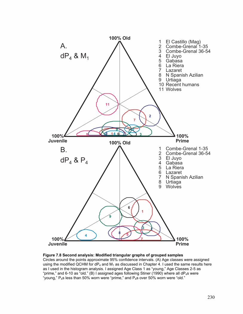
230

Figure 7.8 Second analysis: Modified triangular graphs of grouped samplesCircles around the points approximate 95% confidence intervals. (A) Age classes were assignedusing the modified QCHM for dP4 and M1 as discussed in Chapter 4. I used the same results hereas I used in the histogram analysis. I assigned Age Class 1 as “young,” Age Classes 2-5 as“prime,” and 6-10 as “old.” (B) I assigned ages following Stiner (1990) where all dP4s were“young,” P4s less than 50% worn were “prime,” and P4s over 50% worn were “old.”

100% Old

100%Juvenile

100%Prime

A.

B.

dP4 & M1

dP4 & P4

1 El Castillo (Mag)2 Combe-Grenal 1-353 Combe-Grenal 36-544 El Juyo5 Gabasa6 La Riera7 Lazaret8 N Spanish Azilian9 Urtiaga10 Recent humans11 Wolves

1

2

345 6

7

89 10

11

1 Combe-Grenal 1-352 Combe-Grenal 36-543 El Juyo4 Gabasa5 La Riera6 Lazaret7 N Spanish Azilian8 Urtiaga9 Wolves

100% Old

100%Juvenile

100%Prime

1

23

4 5

6

7

8

9

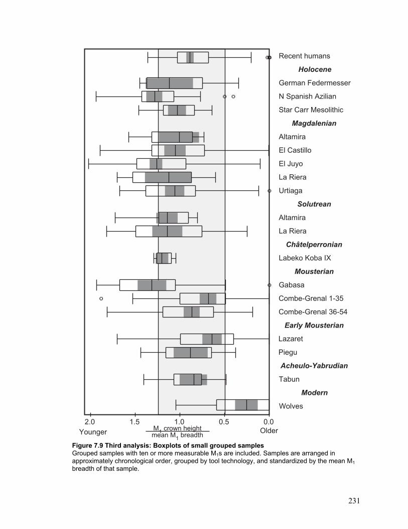
231

Figure 7.9 Third analysis: Boxplots of small grouped samplesGrouped samples with ten or more measurable M1s are included. Samples are arranged inapproximately chronological order, grouped by tool technology, and standardized by the mean M1

breadth of that sample.

Urtiaga

La Riera

El Juyo

El Castillo

Altamira

Labeko Koba IX

Combe-Grenal 36-54

Combe-Grenal 1-35

Gabasa

La Riera

Altamira

Holocene

Magdalenian

Solutrean

Châtelperronian

Mousterian

Early Mousterian

Acheulo-Yabrudian

Wolves

Modern

Tabun

Recent humans

N Spanish Azilian

German Federmesser

Star Carr Mesolithic

M1 crown heightmean M1 breadth

0.00.51.01.52.0OlderYounger

Piegu

Lazaret

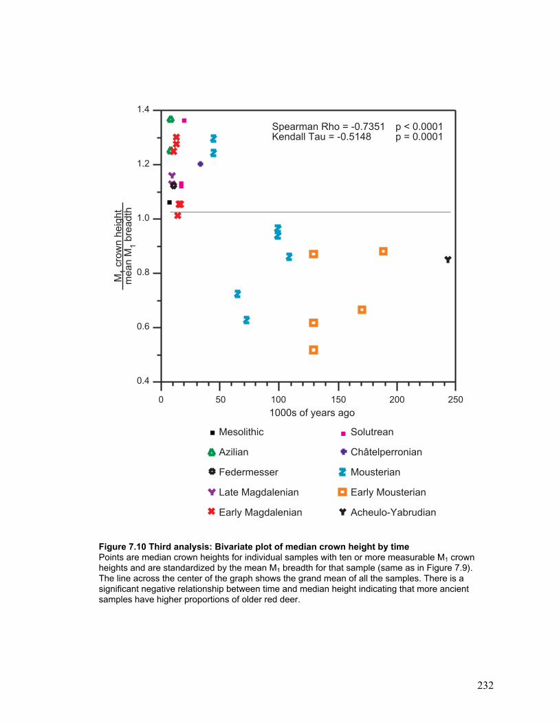
232

Figure 7.10 Third analysis: Bivariate plot of median crown height by timePoints are median crown heights for individual samples with ten or more measurable M1 crownheights and are standardized by the mean M1 breadth for that sample (same as in Figure 7.9).The line across the center of the graph shows the grand mean of all the samples. There is asignificant negative relationship between time and median height indicating that more ancientsamples have higher proportions of older red deer.

Spearman Rho = -0.7351 p < 0.0001Kendall Tau = -0.5148 p = 0.0001

0.4

0.6

0.8

1.0

1.2

1.4

0 50 100 150 200 250

1000s of years ago

M1

crow

n he

ight

mea

n M

1 br

eadt

h

Mesolithic Solutrean

Azilian Châtelperronian

Federmesser Mousterian

Late Magdalenian Early Mousterian

Early Magdalenian Acheulo-Yabrudian

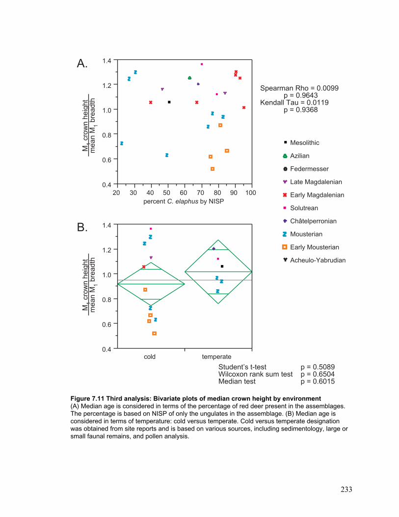
233

Figure 7.11 Third analysis: Bivariate plots of median crown height by environment(A) Median age is considered in terms of the percentage of red deer present in the assemblages.The percentage is based on NISP of only the ungulates in the assemblage. (B) Median age isconsidered in terms of temperature: cold versus temperate. Cold versus temperate designationwas obtained from site reports and is based on various sources, including sedimentology, large orsmall faunal remains, and pollen analysis.

Spearman Rho = 0.0099p = 0.9643

Kendall Tau = 0.0119p = 0.9368

Student’s t-test p = 0.5089Wilcoxon rank sum test p = 0.6504Median test p = 0.6015

percent C. elaphus by NISP

0.4

0.6

0.8

1.0

1.2

1.4

20 30 40 50 60 70 80 90 100

0.4

0.6

0.8

1.0

1.2

1.4

cold temperate

M1

crow

n he

ight

mea

n M

1 br

eadt

hM

1 cr

own

heig

htm

ean

M1

brea

dth

A.

B.

Mesolithic

Azilian

Federmesser

Late Magdalenian

Early Magdalenian

Solutrean

Châtelperronian

Mousterian

Early Mousterian

Acheulo-Yabrudian

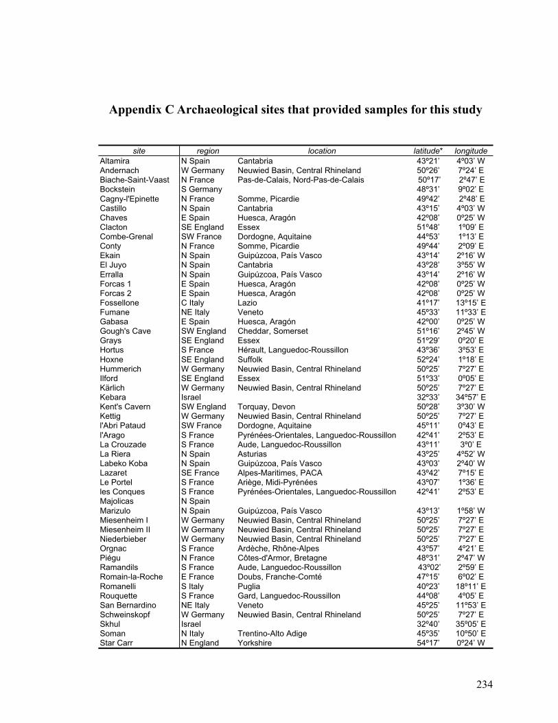
234

Appendix C Archaeological sites that provided samples for this study

site region location latitude* longitudeAltamira N Spain Cantabria 43º21’ 4º03’ WAndernach W Germany Neuwied Basin, Central Rhineland 50º26’ 7º24’ EBiache-Saint-Vaast N France Pas-de-Calais, Nord-Pas-de-Calais 50º17’ 2º47’ EBockstein S Germany 48º31’ 9º02’ ECagny-l'Epinette N France Somme, Picardie 49º42’ 2º48’ ECastillo N Spain Cantabria 43º15’ 4º03’ WChaves E Spain Huesca, Aragón 42º08’ 0º25’ WClacton SE England Essex 51º48’ 1º09’ ECombe-Grenal SW France Dordogne, Aquitaine 44º53’ 1º13’ EConty N France Somme, Picardie 49º44’ 2º09’ EEkain N Spain Guipúzcoa, País Vasco 43º14’ 2º16’ WEl Juyo N Spain Cantabria 43º28’ 3º55’ WErralla N Spain Guipúzcoa, País Vasco 43º14’ 2º16’ WForcas 1 E Spain Huesca, Aragón 42º08’ 0º25’ WForcas 2 E Spain Huesca, Aragón 42º08’ 0º25’ WFossellone C Italy Lazio 41º17’ 13º15’ EFumane NE Italy Veneto 45º33’ 11º33’ EGabasa E Spain Huesca, Aragón 42º00’ 0º25’ WGough's Cave SW England Cheddar, Somerset 51º16’ 2º45’ WGrays SE England Essex 51º29’ 0º20’ EHortus S France Hérault, Languedoc-Roussillon 43º36’ 3º53’ EHoxne SE England Suffolk 52º24’ 1º18’ EHummerich W Germany Neuwied Basin, Central Rhineland 50º25’ 7º27’ EIlford SE England Essex 51º33’ 0º05’ EKärlich W Germany Neuwied Basin, Central Rhineland 50º25’ 7º27’ EKebara Israel 32º33’ 34º57’ EKent's Cavern SW England Torquay, Devon 50º28’ 3º30’ WKettig W Germany Neuwied Basin, Central Rhineland 50º25’ 7º27’ El'Abri Pataud SW France Dordogne, Aquitaine 45º11’ 0º43’ El'Arago S France Pyrénées-Orientales, Languedoc-Roussillon 42º41’ 2º53’ ELa Crouzade S France Aude, Languedoc-Roussillon 43º11’ 3º0’ ELa Riera N Spain Asturias 43º25’ 4º52’ WLabeko Koba N Spain Guipúzcoa, País Vasco 43º03’ 2º40’ WLazaret SE France Alpes-Maritimes, PACA 43º42’ 7º15’ ELe Portel S France Ariège, Midi-Pyrénées 43º07’ 1º36’ Eles Conques S France Pyrénées-Orientales, Languedoc-Roussillon 42º41’ 2º53’ EMajolicas N SpainMarizulo N Spain Guipúzcoa, País Vasco 43º13’ 1º58’ WMiesenheim I W Germany Neuwied Basin, Central Rhineland 50º25’ 7º27’ EMiesenheim II W Germany Neuwied Basin, Central Rhineland 50º25’ 7º27’ ENiederbieber W Germany Neuwied Basin, Central Rhineland 50º25’ 7º27’ EOrgnac S France Ardèche, Rhône-Alpes 43º57’ 4º21’ EPiégu N France Côtes-d'Armor, Bretagne 48º31’ 2º47’ WRamandils S France Aude, Languedoc-Roussillon 43º02’ 2º59’ ERomain-la-Roche E France Doubs, Franche-Comté 47º15’ 6º02’ ERomanelli S Italy Puglia 40º23’ 18º11’ ERouquette S France Gard, Languedoc-Roussillon 44º08’ 4º05’ ESan Bernardino NE Italy Veneto 45º25’ 11º53’ ESchweinskopf W Germany Neuwied Basin, Central Rhineland 50º25’ 7º27’ ESkhul Israel 32º40’ 35º05’ ESoman N Italy Trentino-Alto Adige 45º35’ 10º50’ EStar Carr N England Yorkshire 54º17’ 0º24’ W

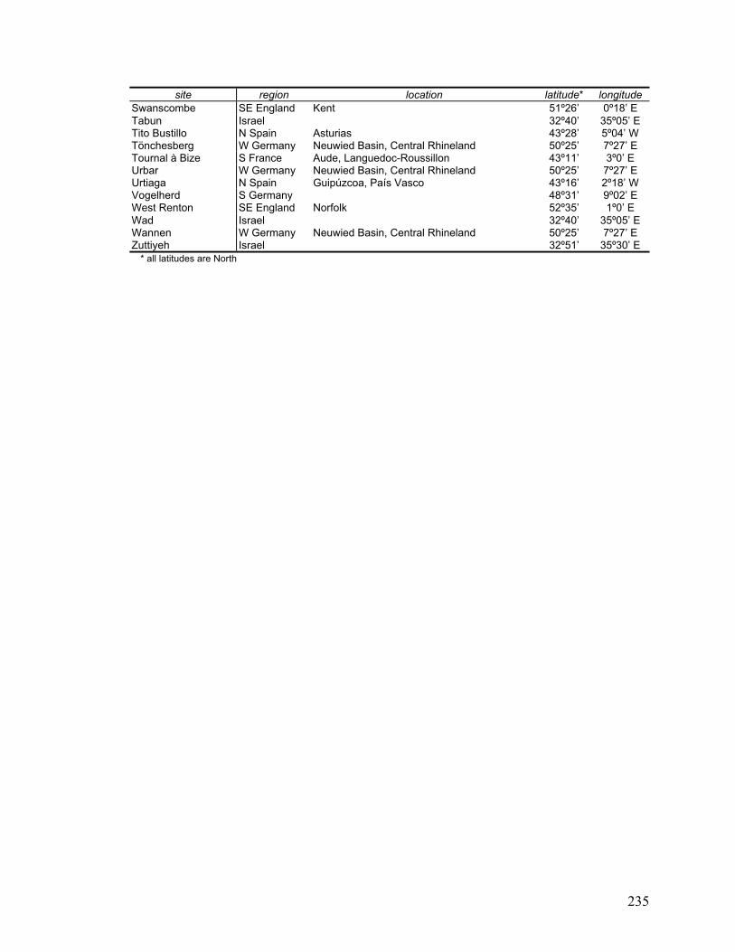
235

site region location latitude* longitudeSwanscombe SE England Kent 51º26’ 0º18’ ETabun Israel 32º40’ 35º05’ ETito Bustillo N Spain Asturias 43º28’ 5º04’ WTönchesberg W Germany Neuwied Basin, Central Rhineland 50º25’ 7º27’ ETournal à Bize S France Aude, Languedoc-Roussillon 43º11’ 3º0’ EUrbar W Germany Neuwied Basin, Central Rhineland 50º25’ 7º27’ EUrtiaga N Spain Guipúzcoa, País Vasco 43º16’ 2º18’ WVogelherd S Germany 48º31’ 9º02’ EWest Renton SE England Norfolk 52º35’ 1º0’ EWad Israel 32º40’ 35º05’ EWannen W Germany Neuwied Basin, Central Rhineland 50º25’ 7º27’ EZuttiyeh Israel 32º51’ 35º30’ E * all latitudes are North

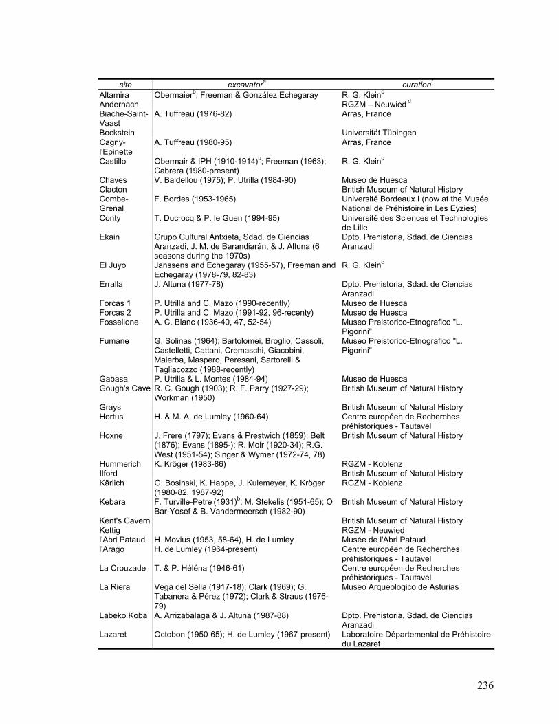
236

site excavatora curationf

Altamira Obermaierb; Freeman & González Echegaray R. G. Kleinc

Andernach RGZM – Neuwied d

Biache-Saint-Vaast

A. Tuffreau (1976-82) Arras, France

Bockstein Universität TübingenCagny-l'Epinette

A. Tuffreau (1980-95) Arras, France

Castillo Obermair & IPH (1910-1914)b; Freeman (1963);Cabrera (1980-present)

R. G. Kleinc

Chaves V. Baldellou (1975); P. Utrilla (1984-90) Museo de HuescaClacton British Museum of Natural HistoryCombe-Grenal

F. Bordes (1953-1965) Université Bordeaux I (now at the MuséeNational de Préhistoire in Les Eyzies)

Conty T. Ducrocq & P. le Guen (1994-95) Université des Sciences et Technologiesde Lille

Ekain Grupo Cultural Antxieta, Sdad. de CienciasAranzadi, J. M. de Barandiarán, & J. Altuna (6seasons during the 1970s)

Dpto. Prehistoria, Sdad. de CienciasAranzadi

El Juyo Janssens and Echegaray (1955-57), Freeman andEchegaray (1978-79, 82-83)

R. G. Kleinc

Erralla J. Altuna (1977-78) Dpto. Prehistoria, Sdad. de CienciasAranzadi

Forcas 1 P. Utrilla and C. Mazo (1990-recently) Museo de HuescaForcas 2 P. Utrilla and C. Mazo (1991-92, 96-recenty) Museo de HuescaFossellone A. C. Blanc (1936-40, 47, 52-54) Museo Preistorico-Etnografico "L.

Pigorini"Fumane G. Solinas (1964); Bartolomei, Broglio, Cassoli,

Castelletti, Cattani, Cremaschi, Giacobini,Malerba, Maspero, Peresani, Sartorelli &Tagliacozzo (1988-recently)

Museo Preistorico-Etnografico "L.Pigorini"

Gabasa P. Utrilla & L. Montes (1984-94) Museo de HuescaGough's Cave R. C. Gough (1903); R. F. Parry (1927-29);

Workman (1950)British Museum of Natural History

Grays British Museum of Natural HistoryHortus H. & M. A. de Lumley (1960-64) Centre européen de Recherches

préhistoriques - TautavelHoxne J. Frere (1797); Evans & Prestwich (1859); Belt

(1876); Evans (1895-); R. Moir (1920-34); R.G.West (1951-54); Singer & Wymer (1972-74, 78)

British Museum of Natural History

Hummerich K. Kröger (1983-86) RGZM - KoblenzIlford British Museum of Natural HistoryKärlich G. Bosinski, K. Happe, J. Kulemeyer, K. Kröger

(1980-82, 1987-92)RGZM - Koblenz

Kebara F. Turville-Petre (1931)b; M. Stekelis (1951-65); OBar-Yosef & B. Vandermeersch (1982-90)

British Museum of Natural History

Kent's Cavern British Museum of Natural HistoryKettig RGZM - Neuwiedl'Abri Pataud H. Movius (1953, 58-64), H. de Lumley Musée de l'Abri Pataudl'Arago H. de Lumley (1964-present) Centre européen de Recherches

préhistoriques - TautavelLa Crouzade T. & P. Héléna (1946-61) Centre européen de Recherches

préhistoriques - TautavelLa Riera Vega del Sella (1917-18); Clark (1969); G.

Tabanera & Pérez (1972); Clark & Straus (1976-79)

Museo Arqueologico de Asturias

Labeko Koba A. Arrizabalaga & J. Altuna (1987-88) Dpto. Prehistoria, Sdad. de CienciasAranzadi

Lazaret Octobon (1950-65); H. de Lumley (1967-present) Laboratoire Départemental de Préhistoiredu Lazaret

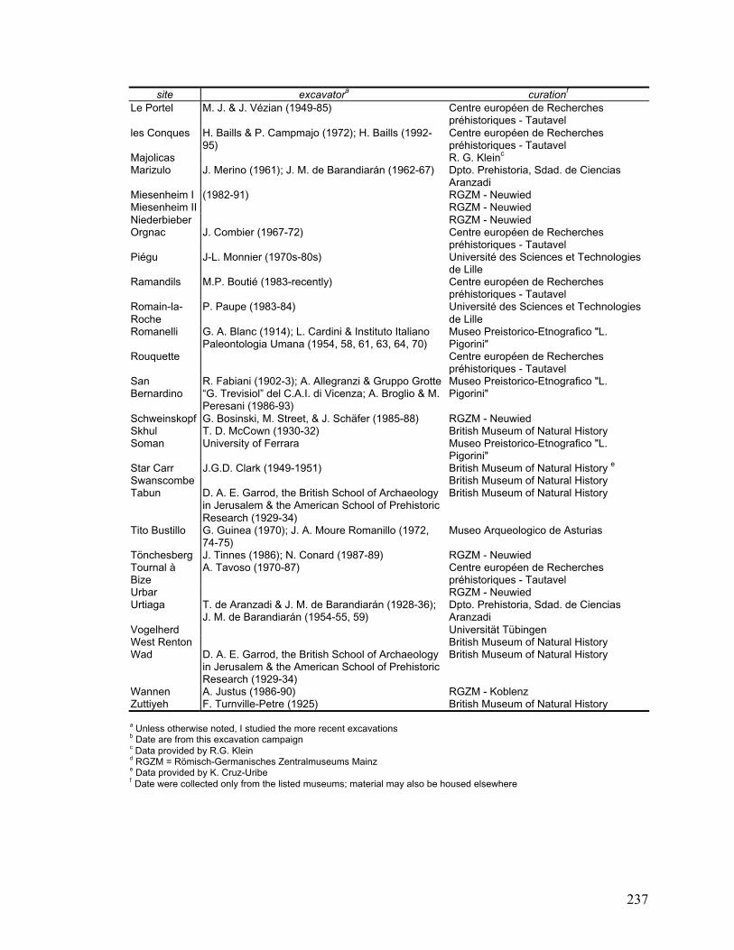
237

site excavatora curationf

Le Portel M. J. & J. Vézian (1949-85) Centre européen de Recherchespréhistoriques - Tautavel

les Conques H. Baills & P. Campmajo (1972); H. Baills (1992-95)

Centre européen de Recherchespréhistoriques - Tautavel

Majolicas R. G. Kleinc

Marizulo J. Merino (1961); J. M. de Barandiarán (1962-67) Dpto. Prehistoria, Sdad. de CienciasAranzadi

Miesenheim I (1982-91) RGZM - NeuwiedMiesenheim II RGZM - NeuwiedNiederbieber RGZM - NeuwiedOrgnac J. Combier (1967-72) Centre européen de Recherches

préhistoriques - TautavelPiégu J-L. Monnier (1970s-80s) Université des Sciences et Technologies

de LilleRamandils M.P. Boutié (1983-recently) Centre européen de Recherches

préhistoriques - TautavelRomain-la-Roche

P. Paupe (1983-84) Université des Sciences et Technologiesde Lille

Romanelli G. A. Blanc (1914); L. Cardini & Instituto ItalianoPaleontologia Umana (1954, 58, 61, 63, 64, 70)

Museo Preistorico-Etnografico "L.Pigorini"

Rouquette Centre européen de Recherchespréhistoriques - Tautavel

SanBernardino

R. Fabiani (1902-3); A. Allegranzi & Gruppo Grotte“G. Trevisiol” del C.A.I. di Vicenza; A. Broglio & M.Peresani (1986-93)

Museo Preistorico-Etnografico "L.Pigorini"

Schweinskopf G. Bosinski, M. Street, & J. Schäfer (1985-88) RGZM - NeuwiedSkhul T. D. McCown (1930-32) British Museum of Natural HistorySoman University of Ferrara Museo Preistorico-Etnografico "L.

Pigorini"Star Carr J.G.D. Clark (1949-1951) British Museum of Natural History e

Swanscombe British Museum of Natural HistoryTabun D. A. E. Garrod, the British School of Archaeology

in Jerusalem & the American School of PrehistoricResearch (1929-34)

British Museum of Natural History

Tito Bustillo G. Guinea (1970); J. A. Moure Romanillo (1972,74-75)

Museo Arqueologico de Asturias

Tönchesberg J. Tinnes (1986); N. Conard (1987-89) RGZM - NeuwiedTournal àBize

A. Tavoso (1970-87) Centre européen de Recherchespréhistoriques - Tautavel

Urbar RGZM - NeuwiedUrtiaga T. de Aranzadi & J. M. de Barandiarán (1928-36);

J. M. de Barandiarán (1954-55, 59)Dpto. Prehistoria, Sdad. de CienciasAranzadi

Vogelherd Universität TübingenWest Renton British Museum of Natural HistoryWad D. A. E. Garrod, the British School of Archaeology

in Jerusalem & the American School of PrehistoricResearch (1929-34)

British Museum of Natural History

Wannen A. Justus (1986-90) RGZM - KoblenzZuttiyeh F. Turnville-Petre (1925) British Museum of Natural History

a Unless otherwise noted, I studied the more recent excavationsb Date are from this excavation campaignc Data provided by R.G. Kleind RGZM = Römisch-Germanisches Zentralmuseums Mainze Data provided by K. Cruz-Uribef Date were collected only from the listed museums; material may also be housed elsewhere

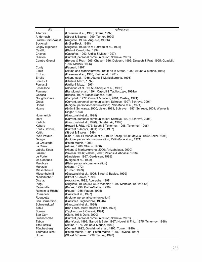
238

site referencesAltamira (Freeman et al., 1988; Straus, 1992)Andernach (Street & Baales, 1999; Turner, 1990)Biache-Saint-Vaast (Auguste, 1995a; Auguste, 1995b)Bockstein (Müller-Beck, 1988)Cagny-l'Epinette (Auguste, 1995c:147; Tuffreau et al., 1995)Castillo (Klein & Cruz-Uribe, 1994)Chaves (Castaños, 1993; Utrilla & Mazo, 1997)Clacton (Currant, personal communication; Schreve, 2001)Combe-Grenal (Bordes & Prat, 1965; Chase, 1986; Delpech, 1996; Delpech & Prat, 1995; Guadelli,

1996; Mellars, 1996)Conty (Fagnart, 1997)Ekain (Altuna and Mariezkurrena (1984) as in Straus, 1992; Altuna & Merino, 1980)El Juyo (Freeman et al., 1988; Klein et al., 1981)Erralla (Altuna et al., 1985; Altuna & Mariezkurrena, 1993)Forcas 1 (Utrilla & Mazo, 1997)Forcas 2 (Utrilla & Mazo, 1997)Fossellone (Alhaique et al., 1995; Alhaique et al., 1996)Fumane (Bartolomei et al., 1994; Cassoli & Tagliacozzo, 1994a)Gabasa (Blasco, 1997; Blasco Sancho, 1995)Gough's Cave (Campbell, 1977; Currant & Jacobi, 2001; Oakley, 1971)Grays (Currant, personal communication; Schreve, 1997; Schreve, 2001)Hortus (Moigne, personal communication; Petit-Marie et al., 1971)Hoxne (Grün & Schwarcz, 2000; Lister, 1993; Schreve, 1997; Schreve, 2001; Wymer &

Singer, 1993)Hummerich (Gaudzinski et al., 1995)Ilford (Currant, personal communication; Schreve, 1997; Schreve, 2001)Kärlich (Gaudzinski et al., 1996); Gaudzinski, 1999)Kebara (Howell & Fritz, 1975; Speth & Tchernov, 1998; Tchernov, 1998)Kent's Cavern (Currant & Jacobi, 2001; Lister, 1987)Kettig (Street & Baales, 1999)l'Abri Pataud (Cho, 1998; El Mansouri et al., 1996; Fellag, 1998; Movius, 1975; Sekhr, 1998)l'Arago (Moigne, personal communication; Petit-Marie et al., 1971)La Crouzade (Patou-Mathis, 1996)La Riera (Altuna, 1986; Straus, 1986)Labeko Koba (Altuna & Mariezkurrena, 2000; Arrizabalaga, 2000)Lazaret (Valensi, 1996; Valensi, 2000; Valensi & Abbassi, 1998)Le Portel (Gardeisen, 1997; Gardeisen, 1999)les Conques (Moigne et al., 1998)Majolicas (Klein, personal communication)Marizulo (Altuna, 1972)Miesenheim I (Turner, 1999)Miesenheim II (Gaudzinski et al., 1995; Street & Baales, 1999)Niederbieber (Street & Baales, 1999)Orgnac (Aouraghe, 1992; Aouraghe, 1999)Piégu (Auguste, 1995a:561-562; Monnier, 1985; Monnier, 1991:53-54)Ramandils (Banes, 1998; Patou-Mathis, 1996)Romain-la-Roche (Paupe, 1985; Paupe, 1995)Romanelli (Cassoli et al., 1997)Rouquette (Moigne, personal communication)San Bernardino (Cassoli & Tagliacozzo, 1994b)Schweinskopf (Gaudzinski et al., 1995)Skhul (Bar-Yosef, 1998; Howell & Fritz, 1975)Soman (Tagliacozzo & Cassoli, 1994)Star Carr (Clark, 1954; Dark, 2000)Swanscombe (Currant, personal communication; Schreve, 2001)Tabun (Bar-Yosef, 1998; Garrod & Bate, 1937; Howell & Fritz, 1975; Tchernov, 1998)Tito Bustillo (Altuna, 1976; Altuna & Merino, 1980)Tönchesberg (Conard, 1992; Gaudzinski et al., 1995; Turner, 1990)Tournal à Bize (Patou-Mathis, 1994; Patou-Mathis, 1996; Tavoso, 1987)Urbar (Street & Baales, 1999; Turner, 1990)

239

site referencesUrtiaga (Altuna, 1972)Vogelherd (Müller-Beck, 1988)West Renton (Lister, 1993; Schreve, 2001)Wad (Garrod & Bate, 1937; Howell & Fritz, 1975)Wannen (Gaudzinski et al., 1995; Justus, 1992)Zuttiyeh (Bar-Yosef, 1998; Howell & Fritz, 1975; Tchernov, 1998)

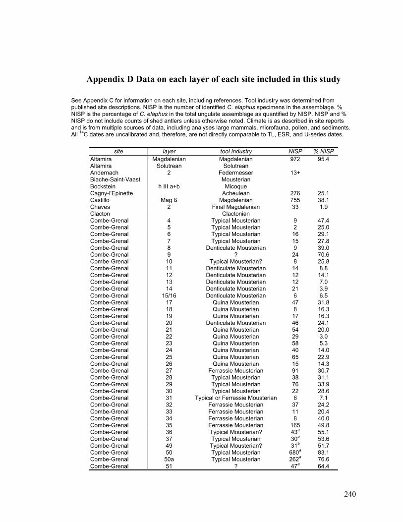
240

Appendix D Data on each layer of each site included in this study

See Appendix C for information on each site, including references. Tool industry was determined frompublished site descriptions. NISP is the number of identified C. elaphus specimens in the assemblage. %NISP is the percentage of C. elaphus in the total ungulate assemblage as quantified by NISP. NISP and %NISP do not include counts of shed antlers unless otherwise noted. Climate is as described in site reportsand is from multiple sources of data, including analyses large mammals, microfauna, pollen, and sediments.All 14C dates are uncalibrated and, therefore, are not directly comparable to TL, ESR, and U-series dates.

site layer tool industry NISP % NISPAltamira Magdalenian Magdalenian 972 95.4Altamira Solutrean SolutreanAndernach 2 Federmesser 13+Biache-Saint-Vaast MousterianBockstein h III a+b MicoqueCagny-l'Epinette Acheulean 276 25.1Castillo Mag ß Magdalenian 755 38.1Chaves 2 Final Magdalenian 33 1.9Clacton ClactonianCombe-Grenal 4 Typical Mousterian 9 47.4Combe-Grenal 5 Typical Mousterian 2 25.0Combe-Grenal 6 Typical Mousterian 16 29.1Combe-Grenal 7 Typical Mousterian 15 27.8Combe-Grenal 8 Denticulate Mousterian 9 39.0Combe-Grenal 9 ? 24 70.6Combe-Grenal 10 Typical Mousterian? 8 25.8Combe-Grenal 11 Denticulate Mousterian 14 8.8Combe-Grenal 12 Denticulate Mousterian 12 14.1Combe-Grenal 13 Denticulate Mousterian 12 7.0Combe-Grenal 14 Denticulate Mousterian 21 3.9Combe-Grenal 15/16 Denticulate Mousterian 6 6.5Combe-Grenal 17 Quina Mousterian 47 31.8Combe-Grenal 18 Quina Mousterian 8 16.3Combe-Grenal 19 Quina Mousterian 17 16.3Combe-Grenal 20 Denticulate Mousterian 46 24.1Combe-Grenal 21 Quina Mousterian 54 20.0Combe-Grenal 22 Quina Mousterian 29 3.0Combe-Grenal 23 Quina Mousterian 58 5.3Combe-Grenal 24 Quina Mousterian 40 14.0Combe-Grenal 25 Quina Mousterian 65 22.9Combe-Grenal 26 Quina Mousterian 15 14.3Combe-Grenal 27 Ferrassie Mousterian 91 30.7Combe-Grenal 28 Typical Mousterian 38 31.1Combe-Grenal 29 Typical Mousterian 76 33.9Combe-Grenal 30 Typical Mousterian 22 28.6Combe-Grenal 31 Typical or Ferrassie Mousterian 6 7.1Combe-Grenal 32 Ferrassie Mousterian 37 24.2Combe-Grenal 33 Ferrassie Mousterian 11 20.4Combe-Grenal 34 Ferrassie Mousterian 8 40.0Combe-Grenal 35 Ferrassie Mousterian 165 49.8Combe-Grenal 36 Typical Mousterian? 43a 55.1Combe-Grenal 37 Typical Mousterian 30a 53.6Combe-Grenal 49 Typical Mousterian? 31a 51.7Combe-Grenal 50 Typical Mousterian 680a 83.1Combe-Grenal 50a Typical Mousterian 262a 76.6Combe-Grenal 51 ? 47a 64.4

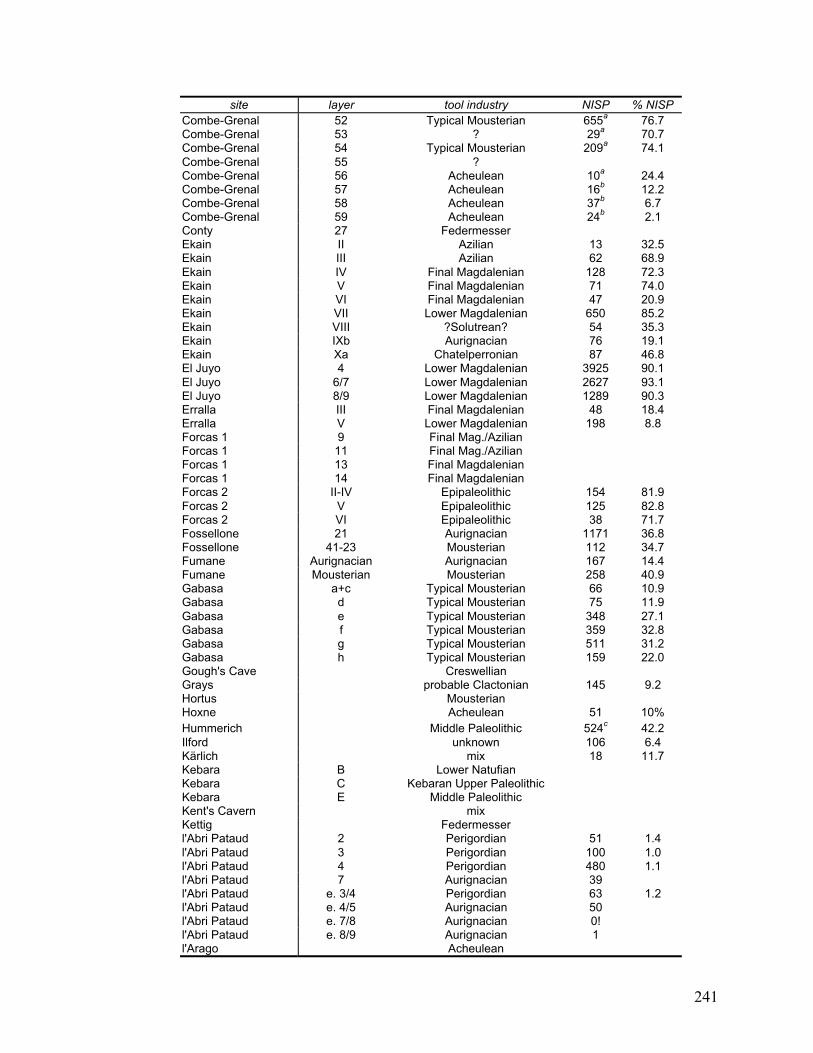
241

site layer tool industry NISP % NISPCombe-Grenal 52 Typical Mousterian 655a 76.7Combe-Grenal 53 ? 29a 70.7Combe-Grenal 54 Typical Mousterian 209a 74.1Combe-Grenal 55 ?Combe-Grenal 56 Acheulean 10a 24.4Combe-Grenal 57 Acheulean 16b 12.2Combe-Grenal 58 Acheulean 37b 6.7Combe-Grenal 59 Acheulean 24b 2.1Conty 27 FedermesserEkain II Azilian 13 32.5Ekain III Azilian 62 68.9Ekain IV Final Magdalenian 128 72.3Ekain V Final Magdalenian 71 74.0Ekain VI Final Magdalenian 47 20.9Ekain VII Lower Magdalenian 650 85.2Ekain VIII ?Solutrean? 54 35.3Ekain IXb Aurignacian 76 19.1Ekain Xa Chatelperronian 87 46.8El Juyo 4 Lower Magdalenian 3925 90.1El Juyo 6/7 Lower Magdalenian 2627 93.1El Juyo 8/9 Lower Magdalenian 1289 90.3Erralla III Final Magdalenian 48 18.4Erralla V Lower Magdalenian 198 8.8Forcas 1 9 Final Mag./AzilianForcas 1 11 Final Mag./AzilianForcas 1 13 Final MagdalenianForcas 1 14 Final MagdalenianForcas 2 II-IV Epipaleolithic 154 81.9Forcas 2 V Epipaleolithic 125 82.8Forcas 2 VI Epipaleolithic 38 71.7Fossellone 21 Aurignacian 1171 36.8Fossellone 41-23 Mousterian 112 34.7Fumane Aurignacian Aurignacian 167 14.4Fumane Mousterian Mousterian 258 40.9Gabasa a+c Typical Mousterian 66 10.9Gabasa d Typical Mousterian 75 11.9Gabasa e Typical Mousterian 348 27.1Gabasa f Typical Mousterian 359 32.8Gabasa g Typical Mousterian 511 31.2Gabasa h Typical Mousterian 159 22.0Gough's Cave CreswellianGrays probable Clactonian 145 9.2Hortus MousterianHoxne Acheulean 51 10%Hummerich Middle Paleolithic 524c 42.2Ilford unknown 106 6.4Kärlich mix 18 11.7Kebara B Lower NatufianKebara C Kebaran Upper PaleolithicKebara E Middle PaleolithicKent's Cavern mixKettig Federmesserl'Abri Pataud 2 Perigordian 51 1.4l'Abri Pataud 3 Perigordian 100 1.0l'Abri Pataud 4 Perigordian 480 1.1l'Abri Pataud 7 Aurignacian 39l'Abri Pataud e. 3/4 Perigordian 63 1.2l'Abri Pataud e. 4/5 Aurignacian 50l'Abri Pataud e. 7/8 Aurignacian 0!l'Abri Pataud e. 8/9 Aurignacian 1l'Arago Acheulean

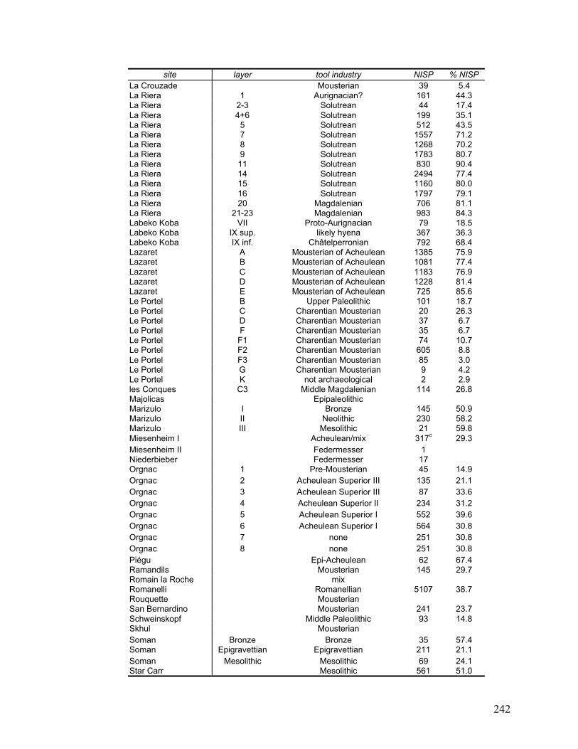
242

site layer tool industry NISP % NISPLa Crouzade Mousterian 39 5.4La Riera 1 Aurignacian? 161 44.3La Riera 2-3 Solutrean 44 17.4La Riera 4+6 Solutrean 199 35.1La Riera 5 Solutrean 512 43.5La Riera 7 Solutrean 1557 71.2La Riera 8 Solutrean 1268 70.2La Riera 9 Solutrean 1783 80.7La Riera 11 Solutrean 830 90.4La Riera 14 Solutrean 2494 77.4La Riera 15 Solutrean 1160 80.0La Riera 16 Solutrean 1797 79.1La Riera 20 Magdalenian 706 81.1La Riera 21-23 Magdalenian 983 84.3Labeko Koba VII Proto-Aurignacian 79 18.5Labeko Koba IX sup. likely hyena 367 36.3Labeko Koba IX inf. Châtelperronian 792 68.4Lazaret A Mousterian of Acheulean 1385 75.9Lazaret B Mousterian of Acheulean 1081 77.4Lazaret C Mousterian of Acheulean 1183 76.9Lazaret D Mousterian of Acheulean 1228 81.4Lazaret E Mousterian of Acheulean 725 85.6Le Portel B Upper Paleolithic 101 18.7Le Portel C Charentian Mousterian 20 26.3Le Portel D Charentian Mousterian 37 6.7Le Portel F Charentian Mousterian 35 6.7Le Portel F1 Charentian Mousterian 74 10.7Le Portel F2 Charentian Mousterian 605 8.8Le Portel F3 Charentian Mousterian 85 3.0Le Portel G Charentian Mousterian 9 4.2Le Portel K not archaeological 2 2.9les Conques C3 Middle Magdalenian 114 26.8Majolicas EpipaleolithicMarizulo I Bronze 145 50.9Marizulo II Neolithic 230 58.2Marizulo III Mesolithic 21 59.8Miesenheim I Acheulean/mix 317c 29.3Miesenheim II Federmesser 1Niederbieber Federmesser 17Orgnac 1 Pre-Mousterian 45 14.9Orgnac 2 Acheulean Superior III 135 21.1Orgnac 3 Acheulean Superior III 87 33.6Orgnac 4 Acheulean Superior II 234 31.2Orgnac 5 Acheulean Superior I 552 39.6Orgnac 6 Acheulean Superior I 564 30.8Orgnac 7 none 251 30.8Orgnac 8 none 251 30.8Piégu Epi-Acheulean 62 67.4Ramandils Mousterian 145 29.7Romain la Roche mixRomanelli Romanellian 5107 38.7Rouquette MousterianSan Bernardino Mousterian 241 23.7Schweinskopf Middle Paleolithic 93 14.8Skhul MousterianSoman Bronze Bronze 35 57.4Soman Epigravettian Epigravettian 211 21.1Soman Mesolithic Mesolithic 69 24.1Star Carr Mesolithic 561 51.0

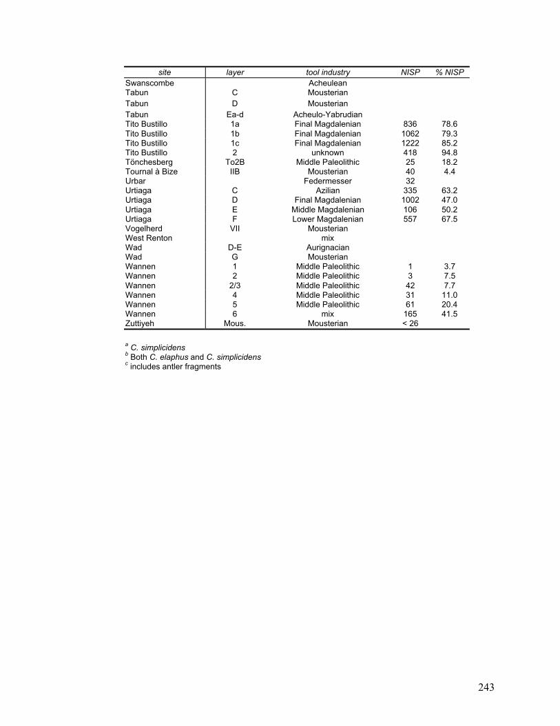
243

site layer tool industry NISP % NISPSwanscombe AcheuleanTabun C MousterianTabun D MousterianTabun Ea-d Acheulo-YabrudianTito Bustillo 1a Final Magdalenian 836 78.6Tito Bustillo 1b Final Magdalenian 1062 79.3Tito Bustillo 1c Final Magdalenian 1222 85.2Tito Bustillo 2 unknown 418 94.8Tönchesberg To2B Middle Paleolithic 25 18.2Tournal à Bize IIB Mousterian 40 4.4Urbar Federmesser 32Urtiaga C Azilian 335 63.2Urtiaga D Final Magdalenian 1002 47.0Urtiaga E Middle Magdalenian 106 50.2Urtiaga F Lower Magdalenian 557 67.5Vogelherd VII MousterianWest Renton mixWad D-E AurignacianWad G MousterianWannen 1 Middle Paleolithic 1 3.7Wannen 2 Middle Paleolithic 3 7.5Wannen 2/3 Middle Paleolithic 42 7.7Wannen 4 Middle Paleolithic 31 11.0Wannen 5 Middle Paleolithic 61 20.4Wannen 6 mix 165 41.5Zuttiyeh Mous. Mousterian < 26

a C. simplicidensb Both C. elaphus and C. simplicidensc includes antler fragments

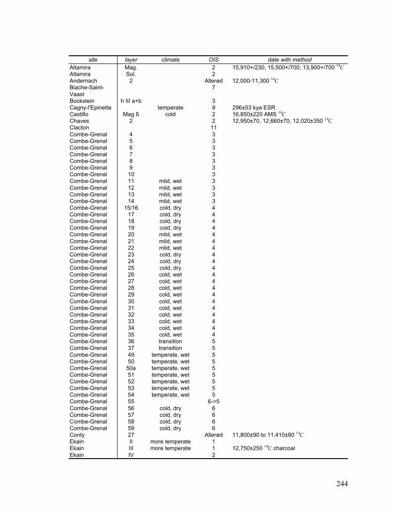
244

site layer climate OIS date with methodAltamira Mag. 2 15,910+/230; 15,500+/700; 13,900+/700 14CAltamira Sol. 2Andernach 2 Allerød 12,000-11,300 14CBiache-Saint-Vaast

7

Bockstein h III a+b 3Cagny-l'Epinette temperate 9 296±53 kya ESRCastillo Mag ß cold 2 16,850±220 AMS 14CChaves 2 2 12,950±70, 12,660±70, 12,020±350 14CClacton 11Combe-Grenal 4 3Combe-Grenal 5 3Combe-Grenal 6 3Combe-Grenal 7 3Combe-Grenal 8 3Combe-Grenal 9 3Combe-Grenal 10 3Combe-Grenal 11 mild, wet 3Combe-Grenal 12 mild, wet 3Combe-Grenal 13 mild, wet 3Combe-Grenal 14 mild, wet 3Combe-Grenal 15/16 cold, dry 4Combe-Grenal 17 cold, dry 4Combe-Grenal 18 cold, dry 4Combe-Grenal 19 cold, dry 4Combe-Grenal 20 mild, wet 4Combe-Grenal 21 mild, wet 4Combe-Grenal 22 mild, wet 4Combe-Grenal 23 cold, dry 4Combe-Grenal 24 cold, dry 4Combe-Grenal 25 cold, dry 4Combe-Grenal 26 cold, wet 4Combe-Grenal 27 cold, wet 4Combe-Grenal 28 cold, wet 4Combe-Grenal 29 cold, wet 4Combe-Grenal 30 cold, wet 4Combe-Grenal 31 cold, wet 4Combe-Grenal 32 cold, wet 4Combe-Grenal 33 cold, wet 4Combe-Grenal 34 cold, wet 4Combe-Grenal 35 cold, wet 4Combe-Grenal 36 transition 5Combe-Grenal 37 transition 5Combe-Grenal 49 temperate, wet 5Combe-Grenal 50 temperate, wet 5Combe-Grenal 50a temperate, wet 5Combe-Grenal 51 temperate, wet 5Combe-Grenal 52 temperate, wet 5Combe-Grenal 53 temperate, wet 5Combe-Grenal 54 temperate, wet 5Combe-Grenal 55 6->5Combe-Grenal 56 cold, dry 6Combe-Grenal 57 cold, dry 6Combe-Grenal 58 cold, dry 6Combe-Grenal 59 cold, dry 6Conty 27 Allerød 11,800±90 to 11,410±80 14CEkain II more temperate 1Ekain III more temperate 1 12,750±250 14C charcoalEkain IV 2

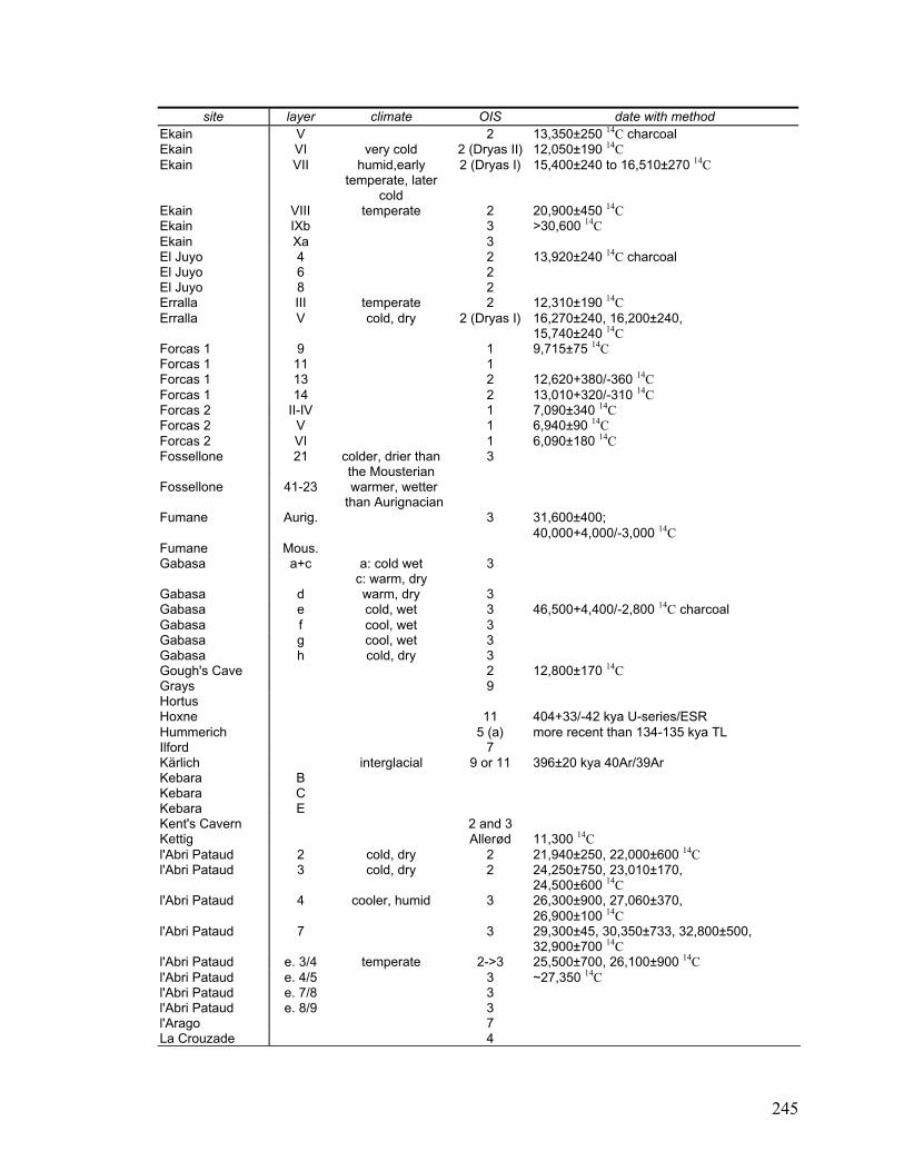
245

site layer climate OIS date with methodEkain V 2 13,350±250 14C charcoalEkain VI very cold 2 (Dryas II) 12,050±190 14CEkain VII humid,early

temperate, latercold

2 (Dryas I) 15,400±240 to 16,510±270 14C

Ekain VIII temperate 2 20,900±450 14CEkain IXb 3 >30,600 14CEkain Xa 3El Juyo 4 2 13,920±240 14C charcoalEl Juyo 6 2El Juyo 8 2Erralla III temperate 2 12,310±190 14CErralla V cold, dry 2 (Dryas I) 16,270±240, 16,200±240,

15,740±240 14CForcas 1 9 1 9,715±75 14CForcas 1 11 1Forcas 1 13 2 12,620+380/-360 14CForcas 1 14 2 13,010+320/-310 14CForcas 2 II-IV 1 7,090±340 14CForcas 2 V 1 6,940±90 14CForcas 2 VI 1 6,090±180 14CFossellone 21 colder, drier than

the Mousterian3

Fossellone 41-23 warmer, wetterthan Aurignacian

Fumane Aurig. 3 31,600±400;40,000+4,000/-3,000 14C

Fumane Mous.Gabasa a+c a: cold wet

c: warm, dry3

Gabasa d warm, dry 3Gabasa e cold, wet 3 46,500+4,400/-2,800 14C charcoalGabasa f cool, wet 3Gabasa g cool, wet 3Gabasa h cold, dry 3Gough's Cave 2 12,800±170 14CGrays 9HortusHoxne 11 404+33/-42 kya U-series/ESRHummerich 5 (a) more recent than 134-135 kya TLIlford 7Kärlich interglacial 9 or 11 396±20 kya 40Ar/39ArKebara BKebara CKebara EKent's Cavern 2 and 3Kettig Allerød 11,300 14Cl'Abri Pataud 2 cold, dry 2 21,940±250, 22,000±600 14Cl'Abri Pataud 3 cold, dry 2 24,250±750, 23,010±170,

24,500±600 14Cl'Abri Pataud 4 cooler, humid 3 26,300±900, 27,060±370,

26,900±100 14Cl'Abri Pataud 7 3 29,300±45, 30,350±733, 32,800±500,

32,900±700 14Cl'Abri Pataud e. 3/4 temperate 2->3 25,500±700, 26,100±900 14Cl'Abri Pataud e. 4/5 3 ~27,350 14Cl'Abri Pataud e. 7/8 3l'Abri Pataud e. 8/9 3l'Arago 7La Crouzade 4

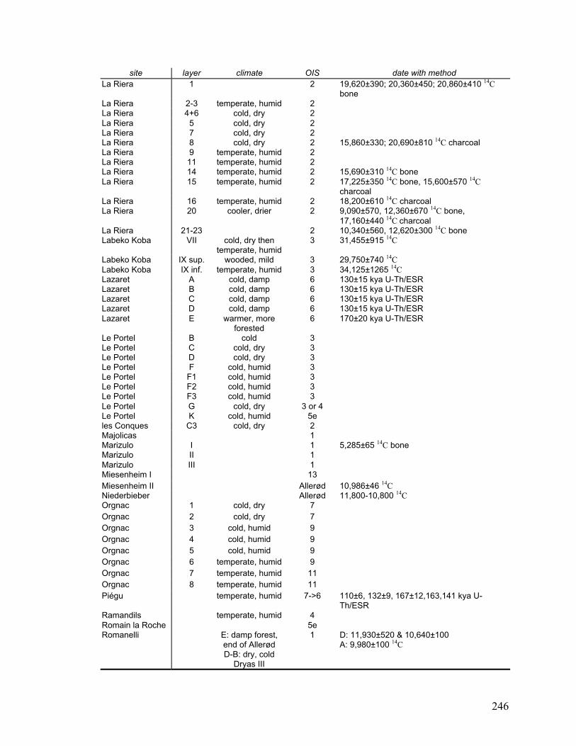
246

site layer climate OIS date with methodLa Riera 1 2 19,620±390; 20,360±450; 20,860±410 14C

boneLa Riera 2-3 temperate, humid 2La Riera 4+6 cold, dry 2La Riera 5 cold, dry 2La Riera 7 cold, dry 2La Riera 8 cold, dry 2 15,860±330; 20,690±810 14C charcoalLa Riera 9 temperate, humid 2La Riera 11 temperate, humid 2La Riera 14 temperate, humid 2 15,690±310 14C boneLa Riera 15 temperate, humid 2 17,225±350 14C bone, 15,600±570 14C

charcoalLa Riera 16 temperate, humid 2 18,200±610 14C charcoalLa Riera 20 cooler, drier 2 9,090±570, 12,360±670 14C bone,

17,160±440 14C charcoalLa Riera 21-23 2 10,340±560, 12,620±300 14C boneLabeko Koba VII cold, dry then

temperate, humid3 31,455±915 14C

Labeko Koba IX sup. wooded, mild 3 29,750±740 14CLabeko Koba IX inf. temperate, humid 3 34,125±1265 14CLazaret A cold, damp 6 130±15 kya U-Th/ESRLazaret B cold, damp 6 130±15 kya U-Th/ESRLazaret C cold, damp 6 130±15 kya U-Th/ESRLazaret D cold, damp 6 130±15 kya U-Th/ESRLazaret E warmer, more

forested6 170±20 kya U-Th/ESR

Le Portel B cold 3Le Portel C cold, dry 3Le Portel D cold, dry 3Le Portel F cold, humid 3Le Portel F1 cold, humid 3Le Portel F2 cold, humid 3Le Portel F3 cold, humid 3Le Portel G cold, dry 3 or 4Le Portel K cold, humid 5eles Conques C3 cold, dry 2Majolicas 1Marizulo I 1 5,285±65 14C boneMarizulo II 1Marizulo III 1Miesenheim I 13Miesenheim II Allerød 10,986±46 14CNiederbieber Allerød 11,800-10,800 14COrgnac 1 cold, dry 7Orgnac 2 cold, dry 7Orgnac 3 cold, humid 9Orgnac 4 cold, humid 9Orgnac 5 cold, humid 9Orgnac 6 temperate, humid 9Orgnac 7 temperate, humid 11Orgnac 8 temperate, humid 11Piégu temperate, humid 7->6 110±6, 132±9, 167±12,163,141 kya U-

Th/ESRRamandils temperate, humid 4Romain la Roche 5eRomanelli E: damp forest,

end of AllerødD-B: dry, cold

Dryas III

1 D: 11,930±520 & 10,640±100A: 9,980±100 14C

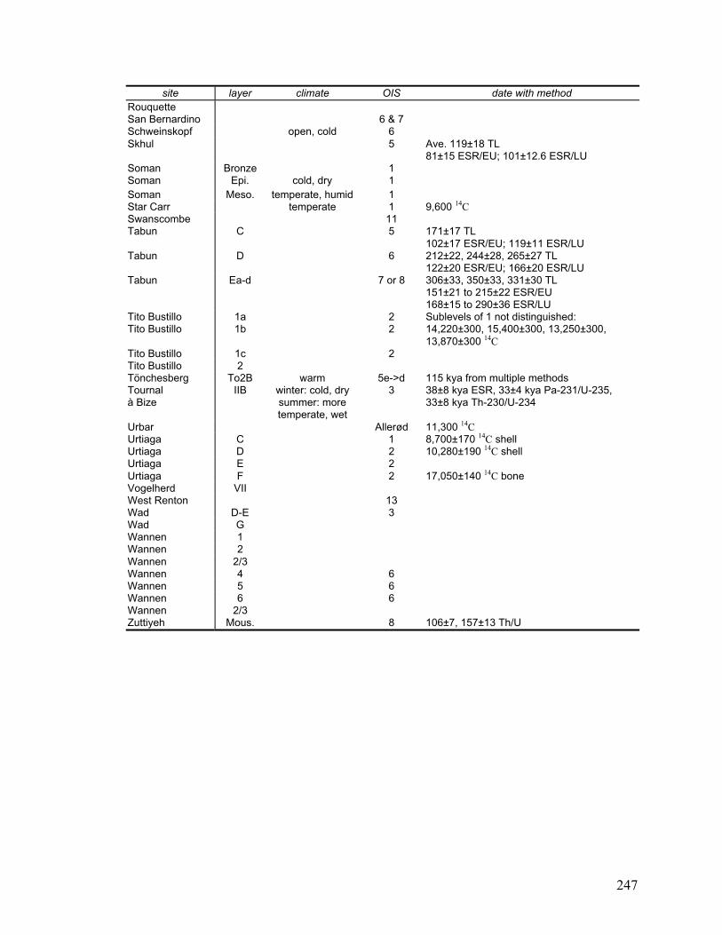
247

site layer climate OIS date with methodRouquetteSan Bernardino 6 & 7Schweinskopf open, cold 6Skhul 5 Ave. 119±18 TL

81±15 ESR/EU; 101±12.6 ESR/LUSoman Bronze 1Soman Epi. cold, dry 1Soman Meso. temperate, humid 1Star Carr temperate 1 9,600 14CSwanscombe 11Tabun C 5 171±17 TL

102±17 ESR/EU; 119±11 ESR/LUTabun D 6 212±22, 244±28, 265±27 TL

122±20 ESR/EU; 166±20 ESR/LUTabun Ea-d 7 or 8 306±33, 350±33, 331±30 TL

151±21 to 215±22 ESR/EU168±15 to 290±36 ESR/LU

Tito Bustillo 1a 2 Sublevels of 1 not distinguished:Tito Bustillo 1b 2 14,220±300, 15,400±300, 13,250±300,

13,870±300 14CTito Bustillo 1c 2Tito Bustillo 2Tönchesberg To2B warm 5e->d 115 kya from multiple methodsTournalà Bize

IIB winter: cold, drysummer: moretemperate, wet

3 38±8 kya ESR, 33±4 kya Pa-231/U-235,33±8 kya Th-230/U-234

Urbar Allerød 11,300 14CUrtiaga C 1 8,700±170 14C shellUrtiaga D 2 10,280±190 14C shellUrtiaga E 2Urtiaga F 2 17,050±140 14C boneVogelherd VIIWest Renton 13Wad D-E 3Wad GWannen 1Wannen 2Wannen 2/3Wannen 4 6Wannen 5 6Wannen 6 6Wannen 2/3Zuttiyeh Mous. 8 106±7, 157±13 Th/U

248

Bibliography

Adams, A. W. (1982). Migration. In (J. W. Thomas & D. E. Toweill, Eds) Elk of NorthAmerica: Ecology and Management. Stackpole Books: Harrisburg, PA, pp. 301-321.

Alhaique, F., Bietti, A., Biondi, S., Cassoli, P. F., Tagliacozzo, A. & Vitagliano, S.(1995). Grotta del Fossellone (San Felice Circeo, Latina). In (A. Bietti & R.Grifoni Cremonesi, Eds) Guide Archeologiche: Preistoria e Protostoria in Italia.Volume 10 - Lazio e Abruzzo. A.B.A.C.O. srl: Forlì, pp. 115-121.

Alhaique, F., Biondi, S., Cassoli, P. F., Recchi, A. & Tagliacozzo, A. (1996).Modification in the exploitation of animal resources between the MiddlePaleolithic and the Aurignacian at Grotta del Fossellone (Monte Circeo, Italy).Proceedings of the XIII U.I.S.P.P. Congress 2, 571-576.

Altuna, J. (1972). Fauna de mamíferos de los yacimientos prehistóricos de Guipuzcoa.Munibe 24, 1-464.

Altuna, J. (1976). Los Mamiferos del Yacimiento Prehistorico de Tito Bustillo (Asturias).Oviedo: Instituto de Estudios Asturianos.

Altuna, J. (1986). The mammalian faunas from the prehistoric site of La Riera. In (L. G.Straus & G. A. Clark, Eds) La Riera Cave: Stone Age Hunter-GathererAdaptations in Northern Spain. Anthropological Research Papers: Arizona StateUniversity, pp. 327-274, 421-477.

Altuna, J., Baldeon, A. & Mariezkurrena, K. (1985). Cazadores magdalenienses enErralla (Cestona, País Vasco). Munibe 37, 1-206.

Altuna, J. & Mariezkurrena, K. (1993). Faunes de mammifères des gisementsMagdaléniens du Pays Basque et zones limitrophes. Congrès National dessociétés historiques et scientifiques 118 PAU, 149-162.

Altuna, J. & Mariezkurrena, K. (2000). Macromamíferos del yacimiento de Labeko Koba(Arrasate, País Vasco). Munibe 52, 107-181.

Altuna, J. & Merino, J. M. (1980). El Yacimiento Prehistorico de la Cueva de Ekain(Deba, Guipúzcoa). San Sebastian: Eusko Ikaskuntza. Sociedad de EstudiosVascos.

Ambrose, S. H. (1998). Chronology of the Later Stone Age and food production in EastAfrica. Journal of Archaeological Science 25, 377-392.

249

Amorosi, T. (1989). A Postcranial Guide to Domestic Neo-Natal and Juvenile Mammals.(Vol. 533). Oxford: BAR International Series.

Aouraghe, H. (1992). Les Faunes des Grands Mammifères du Site Pléistocène Moyend'Orgnac 3 (Ardèche, France). Etude paléontologique et palethnographique.Implications paléoécologiques et biostratigraphiques. Ph.D. Thesis, MuséumNational d'Histoire Naturelle, Paris.

Aouraghe, H. (1999). Nouvelle reconstitution de paléoenvironnement par les grandsmammifères: les faunes du Pléistocène Moyen d'Orgnac 3 (Ardèche, France).L'Anthropologie 103, 177-184.

Arrizabalaga, A. (2000). El yacimiento arqueológico de Labeko Koba (Arrasate, PaísVasco). Entorno. Crónica de las investigaciones. Estratigrafía y estructuras.Cronología absoluta. Munibe 52, 15-72.

Ashton, K. G., Tracy, M. C. & de Queiroz, A. (2000). Is Bergmann's rule valid formammals? The American Naturalist 156, 390-415.

Auguste, P. (1995a). Cadres Biostratigraphiques et Paléoécologiques du PeuplementHumain dans la France Septentrionale durant le Pléistocene. Apports de l'ÉtudePaléontologique des Grands Mammiferes du Gisement de Biache-Saint-Vaast(Pas-de-Calais). Ph.D. Thesis, Museum National d'Histoire Naturelle, Paris.

Auguste, P. (1995b). Chasse et charognage au Paléolithique Moyen: L'apport dugisement de Biache-Saint-Vaast (Pas-de-Calais). Bulletin de la Sociétépréhistorique française 92, 155-167.

Auguste, P. (1995c). Révision préliminaire des grands mammifères des gisement duPaléolithique Inférieur et Moyen de la Vallée de la Somme. Bulletin de la Sociétépréhistorique française 92, 143-154.

Banes, L. (1998). La Faune Mousterienne de la Grotte des Ramandils (La Nouvelle,Aude). Memoire de D.E.A. Thesis, Université de Perpignan, Perpignan.

Bar-Yosef, O. (1998). The chronology of the Middle Paleolithic of the Levant. In (T.Akazawa, K. Aoki & O. Bar-Yosef, Eds) Neandertals and Modern Humans inWestern Asia. Plenum Press: New York, pp. 39-56.

Bar-Yosef, O. (2000). A Mediterranean perspective on the Middle/Upper Palaeolithicrevolution. In (C. B. Stringer, R. N. E. Barton & J. C. Finlayson, Eds)Neanderthals on the Edge. Oxbow Books: Oxford, pp. 9-18.

Bartolomei, G., Broglio, A., Cassoli, P. F., Castelletti, L., Cattani, L., Cremaschi, M.,Giacobini, G., Malerba, G., Maspero, A., Peresani, M., Sartorelli, A. &Tagliacozzo, A. (1994). La Grotte de Fumane. Un site aurignacien au pied desAlpes. Preistoria Alpina - Museo Tridentino di Scienze Naturali 28, 131-179.

250

Bartram, L. E. (1993). Perspectives on skeletal part profiles and utility curves fromeastern Kalahari ethnoarchaeology. In (J. Hudson, Ed.) From Bones to Behavior:Ethnoarchaeological and Experimental Contributions to the Interpretation ofFaunal Remains. Center for Archaeological Investigations, Southern IllinoisUniversity: Carbondale, IL, pp. 115-137.

Binford, L. R. (1985). Human ancestors: Changing views of their behavior. Journal ofAnthropological Archaeology 4, 292-327.

Binford, L. R. (1988). Etude taphonomique des restes fauniques de la grotte Vaufrey. In(J.-P. Rigaud, Ed.) La Grotte Vaufrey à Cénac et Saint-Julien (Dordogne):Paléoenvironnements, Chronologie et Activités Humaines. Mémoires de laSociété Préhistorique Française 19, pp. 535-564.

Binford, L. R. & Bertram, J. B. (1977). Bone frequencies and attritional processes. In (L.R. Binford, Ed.) For Theory Building in Archaeology. Academic Press: NewYork, pp. 77-153.

Blasco, M. F. (1997). In the pursuit of game: The Mousterian cave site of Gabasa I in theSpanish Pyrennes. Journal of Anthropological Research 53, 177-217.

Blasco Sancho, M. F. (1995). Hombres, Fieras y Presas: Estudio arqueozoológico ytafonómico del yacimiento del Paleolítico Medio de las Cueva de Gabasa 1(Huesca). Dpto. Ciencias de la Antigüedad (Area de Prehistoria), Universidad deZaragoza: Monografías Arqueológicas 38, 1-205.

Blumenschine, R. J. (1987). Characteristics of an Early Hominid Scavenging Niche.Current Anthropology 28, 383-407.

Bocquet-Appel, J.-P. & Demars, P.-Y. (2000a). Neanderthal contraction and modernhuman colonization of Europe. Antiquity 74, 544-552.

Bocquet-Appel, J.-P. & Demars, P.-Y. (2000b). Population kinetics in the UpperPalaeolithic in western Europe. Journal of Archaeological Science 27, 551-570.

Boëda, E., Connan, J., Dessort, D., Muhesen, S., Mercier, N., Valladas, H. & Tisnérat, N.(1996). Bitumen as a hafting material on Middle Palaeolithic artefacts. Nature380, 336-338.

Bordes, F. & Prat, F. (1965). Observations sur les faunes du Riss et du Würm I enDordogne. L'Anthropologie 69, 31-46.

Boyd, D. K., Ream, R. R., Pletscher, D. H. & Fairchild, M. W. (1994). Prey taken bycolonizing wolves and hunters in the Glacier National Park area. Journal ofWildlife Management 58, 289-295.

Boyle, K. (1990). Upper Palaeolithic Faunas from South-West France. (Vol. 557).Oxford: BAR International Series.

251

Boyle, K. (1998). The Middle Palaeolithic Geography of Southern France: Resourcesand Site Location. (Vol. 723). Oxford: Archaeopress.

Bradley, R. S. (1999). Paleoclimatology: Reconstructing Climates of the Quaternary. SanDiego: Academic Press.

Bräuer, G. (1989). The evolution of modern humans: a comparison of the African andnon-African evidence. In (P. Mellars & C. B. Stringer, Eds) The HumanRevolution: Behavioural and Biological Perspectives on the Origins of ModernHumans. Edinburgh University Press: Edinburgh, pp. 123-154.

Brown, W. A. B. & Chapman, N. G. (1991a). Age assessment of red deer (Cervuselaphus): from a scoring scheme based on radiographs of developing permanentmolariform teeth. Journal of Zoology, London 225, 85-97.

Brown, W. A. B. & Chapman, N. G. (1991b). The dentition of red deer (Cervus elaphus):a scoring scheme to assess age from wear of the permanent molariform teeth.Journal of Zoology, London 224, 519-536.

Brugal, J.-P. & David, F. (1993). Usure dentaire, courbe de mortalité et "saisonnalité": lesgisements du Paléolithique moyen à bovidés. In Exploitation des AnimauxSauvages a Travers le Temps. APDCA: Juan-les-Pins, France, pp. 63-77.

Bryant, L. D. & Maser, C. (1982). Classification and distribution. In (J. W. Thomas & D.E. Toweill, Eds) Elk of North America: Ecology and Management. StackpoleBooks: Harrisburg, PA, pp. 1-59.

Bunn, H. T. (1993). Bone assemblage at base camps: A further consideration of carcasstransport and bone destruction by the Hadza. In (J. Hudson, Ed.) From Bones toBehavior: Ethnoarchaeological and Experimental Contributions to theInterpretation of Faunal Remains. Center for Archaeological Investigations,Southern Illinois University: Carbondale, IL, pp. 156-168.

Burke, A. (1995). Prey Movements and settlement patterns during the Upper Palaeolithicin Southwestern France. (Vol. 619). Oxford: BAR International Series.

Cabrera, V., Pike-Tay, A., Lloret, M. & Bernaldo de Quirós, F. (2000). Continuitypatterns in the Middle-Upper Palaeolithic transition in Cantabrian Spain. In (C. B.Stringer, R. N. E. Barton & J. C. Finlayson, Eds) Neanderthals on the Edge.Oxbow Books: Oxford, pp. 85-93.

Campbell, J. B. (1977). The Upper Paleolithic of Britain: A Study of Man and Nature inthe Late Ice Age. (Vol. 1). Oxford: Clarendon Press.

Cann, R. L., Stoneking, M. & Wilson, A. C. (1987). Mitochondrial DNA and humanevolution. Nature 325, 31-36.

252

Carbyn, L. N. (1983). Wolf predation on elk in Riding Mountain National Park,Manitoba. Journal of Wildlife Management 47, 963-976.

Cassoli, P. F., Fiore, I. & Tagliacozzo, A. (1997). Butchery and exploitation of largemammals in the Epigravettian levels of Grotta Romanelli (Apulia, Italy).Anthropozoologica 25, 26, 309-318.

Cassoli, P. F. & Tagliacozzo, A. (1994a). Considerazioni paleontologiche,paleoecologiche e archeozoologiche sui macromammiferi e gli uccelli dei livellidel Pleistocene Superiore del Riparo de Fumane (VR) (Scavi 1988-91). Boll. Mus.civ. St. nat. Verona 18, 349-445.

Cassoli, P. F. & Tagliacozzo, A. (1994b). I resti ossei di macromammiferi, uccelli e pescidella Grotta Maggiore di San Bernardino sui Colli Berici (VI): considerazionipaleoeconomiche, paleoecologiche e cronologiche. Bullettino di PaletnologiaItaliana (Roma) 85, 1-71.

Castaños, P. (1993). Estudio de los macromamíferos de los niveles paleolíticos deChaves. Bolskan: Revista de Arqueología del Instituto de EstudiosAltoaragoneses 10, 9-30.

Caughley, G. (1966). Mortality patterns in mammals. Ecology 47, 906-918.

Caughley, G. (1977). Analysis of Vertebrate Populations. London: John Wiley & Sons.

Chase, P. G. (1986). The Hunters of Combe-Grenal: Approaches to Middle PaleolithicSubsistence in Europe. (Vol. 286). Oxford: BAR International Series.

Chase, P. G. (1989). How different was Middle Palaeolithic subsistence? Azooarchaeological perspective on the Middle to Upper Palaeolithic transition. In(P. Mellars & C. B. Stringer, Eds) The Human Revolution: Behavioural andBiological Perspectives on the Origins of Modern Humans. Edinburgh UniversityPress: Edinburgh, pp. 321-337.

Cho, T.-S. (1998). Etude Archeozoologique de la Faune du Perigordien Superieur(couches 2, 3 et 4) de l'Abri Pataud (Les Eyzies, Dordogne): Paléoécologie,Taphonomie, Paleoeconomie. Ph.D. Thesis, Museum National d'HistoireNaturelle, Paris.

Churchill, S. E. & Smith, F. H. (2000). Makers of the Early Aurignacian of Europe.Yearbook of Physical Anthropology 43, 61-115.

Clark, G. A. & Straus, L. G. (1983). Late Pleistocene hunter-gatherer adaptations inCantabrian Spain. In (G. Bailey, Ed.) Hunter-Gatherer Economy in Prehistory.Cambridge University Press: Cambridge, pp. 131-148.

Clark, J. G. D. (1954). Excavations at Star Carr. Cambridge: Cambridge UniversityPress.

253

Clutton-Brock, T. H. & Albon, S. D. (1983). Climatic variation and body weight of reddeer. Journal of Wildlife Management 47, 1197-1201.

Clutton-Brock, T. H. & Albon, S. D. (1989). Red deer in the Highlands. Oxford: BSPProfessional.

Clutton-Brock, T. H., Coulson, T. N., Milner-Gulland, E. J., Thomson, D. & Armstrong,H. M. (2002). Sex differences in emigration and mortality affect optimalmanagement of deer populations. Nature 415, 633-637.

Clutton-Brock, T. H., Guinness, F. E. & Albon, S. D. (1982). Red deer: behavior andecology of two sexes. Chicago: University of Chicago Press.

Conard, N. J. (1992). Tönchesberg and its position in the Paleolithic prehistory ofNorthern Europe. Monographien des Römisch-Germanischen Zentralmuseum 20.

Cruz-Uribe, K. (1991). Distinguishing hyena from hominid bone accumulations. Journalof Field Archaeology 18, 467-486.

Currant, A. & Jacobi, R. (2001). A formal mammalian biostratigraphy for the LatePleistocene of Britain. Quaternary Science Reviews 20, 1707-1716.

d'Errico, F., Henshilwood, C. S. & Soressi, M. (2002, March 22, 2002). New evidence forsymbolism and behavioural modernity in the MSA and Mousterian. Paperpresented at the Society for American Archaeology, Denver, CO.

d'Errico, F. & Soressi, M. (2002). Systematic use of manganese pigment by Pech-de-l'Azé Neandertals: implications for the origin of behavioral modernity. Journal ofHuman Evolution 42, A13.

d'Errico, F., Zilhão, J., Julien, M., Baffier, D. & Pelegrin, J. (1998). Neanderthalacculturation in western Europe? A critical review of the evidence and itsinterpretation. Current Anthropology 39, S1-S44.

Dark, P. (2000). Revised 'absolute' dating of the early Mesolithic site of Star Carr, NorthYorkshire, in the light of changes in the early Holocene tree-ring chronology.Antiquity 74, 304-307.

Davies, W., Stewart, J. & van Andel, T. H. (2000). Neandertal landscapes - a preview. In(C. B. Stringer, R. N. E. Barton & J. C. Finlayson, Eds) Neanderthals on theEdge. Oxbow Books: Oxford, pp. 1-8.

Dayan, T., Simberloff, D., Tchernov, E. & Yom-Tov, Y. (1991). Calibrating thepaleothermometer: climate, communities, and the evolution of size. Paleobiology17, 189-199.

254

Deacon, H. J. (1989). Late Pleistocene palaeoecology and archaeology in the SouthernCape, South Africa. In (P. Mellars & C. B. Stringer, Eds) The Human Revolution:Behavioural and Biological Perspectives on the Origins of Modern Humans.Edinburgh University Press: Edinburgh, pp. 547-564.

Deevey, E. S. (1947). Life tables for natural populations of animals. Quarterly Review ofBiology 22, 283-314.

Delpech, F. (1983). Les Faunes du Paléolithique Supérieur deans le Sud-Ouest de laFrance. Paris: CNRS.

Delpech, F. (1996). L'environnement animal des Mousteriens Quina du Perigord. Paleo8, 31-46.

Delpech, F. & Prat, F. (1995). Nouvelles observations sur les faunes Acheuléennes deCombe Grenal (Domme, Dordogne). Paleo 7, 123-137.

Dixon, S. L. & Lyman, R. L. (1996). On the Holocene history of elk (Cervus elaphus) ineastern Washington. Northwest Science 70, 262-272.

Dolukhanov, P., Sokoloff, D. & Shukurov, A. (2001). Radiocarbon chronology of UpperPalaeolithic sites in eastern Europe at improved resolution. Journal ofArchaeological Science 28, 699-712.

Driesch, v. d. (1976). A Guide to the Measurement of Animal Bones fromArchaeological Sites. Bulletin of the Peabody Museum of Archaeology andEthnology (Harvard University) 1, 1-136.

Duarte, C., Maurícia, J., Pettitt, P. B., Souto, R., Trinkaus, E., van der Plicht, H. &Zilhão, J. (1999). The early Upper Paleolithic human skeleton from the Abrigo doLagar Velho (Portugal) and modern human emergence in Iberia. Proceedings ofthe National Academy of Science 96, 7604-7609.

Ducos, P. (2000). A new approach to the construction of age profiles. ArchaeoZoologia11, 135-144.

Efron, B. & Tibshirani, R. J. (1993). An Introduction to the Bootstrap. (Vol. 57). NewYork: Chapman & Hall.

El Mansouri, M., El Fouikar, A. & Saint-Martin, B. (1996). Correlation Between 14CAges and Aspartic Acid Racemization at the Upper Palaeolithic Site of the AbriPataud (Dordogne, France). Journal of Archaeological Science 23, 803-809.

Enloe, J. G. (1993). Subsistence organization in the Early Upper Paleolithic: Reindeerhunters of the Abri du Flageolet, Couche V. In (H. Knecht, A. Pike-Tay & R.White, Eds) Before Lascaux: The Complex Record of the Early Upper Paleolithic.CRC Press: Boca Raton, pp. 101-115.

255

Fagnart, J.-P. (1997). Le Gisement du Maraise de Conty (Somme). Mémoires de laSociété Préhistorique Française 24, 108-119.

Falgueres, C., Bahain, J., Yokoyama, Y., Arsuaga, J., de Castro, J., Carbonell, E.,Bischoff, J. & Dolo, J. (1999). Earliest humans in Europe: the age of TD6 GranDolina, Atapuerca, Spain. Journal of Human Evolution 37, 343-352.

Farizy, C., David, J., Jaubert, J., Eisenmann, V., Girard, M., Grün, R., Krier, V., Leclerc,J., Miskovsky, J.-C. & Simonnet, R. (1994). Hommes et bisons du Paléolithiquemoyen à Mauran (Haute-Garonne). Paris: CNRS Editions.

Fellag, H. (1998). Apport de l'analyse pollinique à la connaissance dupaléoenvironnement du Paléolithique supérieur de l'abri Pataud (Dordogne,France). Bulletin de la Société préhistorique française 95, 171-181.

Flook, D. R. (1970). Causes and implications of an observed sex differential in thesurvival of wapiti. Canadian Wildlife Service Report Series 11, 1-71.

Frayer, D. W. (1992). The persistence of Neanderthal features in post-NeanderthalEuropeans. In (G. Bräuer & F. H. Smith, Eds) Continuity or Replacement:Controversies in Homo sapiens evolution. A.A. Balkema: Rotterdam, pp. 179-189.

Freeman, L. G., González Echegaray, J., Klein, R. G. & Crowe, W. T. (1988).Dimensions of research at El Juyo. In (H. L. Dibble & A. Montet-White, Eds)Upper Pleistocene Prehistory of Western Eurasia. The University Museum:Philadelphia, pp. 3-39.

Frison, G. C. (1987). Prehistoric, plains-mountain, large-mammal, communal huntingstrategies. In (M. H. Nitecki & D. V. Nitecki, Eds) The Evolution of HumanHunting. Plenum Press: New York, pp. 177-223.

Frison, G. C. (1991a). Hunting strategies, prey behavior and mortality data. In (M. C.Stiner, Ed.) Human Predators and Prey Mortality. Westview Press: Boulder, CO,pp. 15-30.

Frison, G. C. (1991b). Prehistoric Hunters of the High Plains. San Diego: AcademicPress.

Gambier, D. (1989). Fossil hominids from the early Upper Paleolithic (Aurignacian) ofFrance. In (P. Mellars & C. B. Stringer, Eds) The Human Revolution: Behaviouraland Biological Perspectives on the Origins of Modern Humans. EdinburghUniversity Press: Edinburgh, pp. 194-211.

Gamble, C. (1999). The Palaeolithic Societies of Europe. Cambridge: CambridgeUniversity Press.

256

Gardeisen, A. (1997). La grotte ouest du Portel, Ariège, France: Restes fauniques etstratégies de chasse dans le Pléistocène supérieur pyrénéen. (Vol. 673). Oxford:BAR International Series.

Gardeisen, A. (1999). Middle Palaeolithic subsistence in the West Cave if "Le Portel"(Pyrénées, France). Journal of Archaeological Science 26, 1145-1158.

Garrod, D. A. E. & Bate, D. M. A. (1937). The Stone Age of Mount Carmel: Excavationsat the Wady El-Mughara. (Vol. 1). Oxford: The Calendon Press.

Gaudzinski, S. (1995). Wallertheim revisited: a Re-analysis of the fauna from the MiddlePalaeolithic site of Wallertheim (Rheinhessen/Germany). Journal ofArchaeological Science 22, 51-66.

Gaudzinski, S. (1996). On bovid assemblages and their consequences for the knowledgeof subsistence patterns in the Middle Paleolithic. Proceedings of the PrehistoricSociety 62, 19-39.

Gaudzinski, S. (1999). Considerations on the taphonomy of the faunal assemblage fromthe Middle Pleistocene Kärlich-Seeufer site (Central Rhineland, Germany).Monographien des Römisch-Germanischen Zentralmuseum 42, 139-151.

Gaudzinski, S., Bittmann, F., Boenigk, W., Frechen, M. & van Kolfschoten, T. (1996).Palaeoecology and archaeology of the Kärlich-Seeufer open-air site (MiddlePleistocene) in the Central Rhineland, Germany. Quaternary Research 46, 319-334.

Gaudzinski, S., Street, M. & Turner, E. (1995). Middle and Upper Pleistocene hominidoccupation in the Neuwied Basin (Rhineland). In (W. Schirmer, Ed.) QuaternaryField Trips in Central Europe. Verlag Dr. Friedrich Pfeil: München, pp. 1449-1475.

Geist, V. (1982). Adaptive behavioral strategies. In (J. W. Thomas & D. E. Toweill, Eds)Elk of North America: Ecology and Management. Stackpole Books: Harrisburg,PA, pp. 219-277.

Geist, V. (1998). Deer of the World: Their Evolution, Behavior, and Ecology.Mechanicsburg, PA: Stackpole Books.

Gifford-Gonzalez, D. (1991). Examining and refining the Quadratic Crown HeightMethod of Age Estimation. In (M. C. Stiner, Ed.) Human Predators and PreyMortality. Westview Press: Boulder, CO, pp. 41-78.

Grayson, D. K. & Delpech, F. (1994). The evidence for Middle Palaeolithic scavengingfrom Couche VIII, Grotte Vaufrey (Dordogne, France). Journal of ArchaeologicalScience 21, 359-375.

257

Grayson, D. K. & Delpech, F. (1998). Changing diet breadth in the Early UpperPalaeolithic of Southwestern France. Journal of Archaeological Science 25, 1119-1129.

Grayson, D. K. & Delpech, F. (2002, March 21, 2002). Specialized Early UpperPaleolithic hunters in Southwestern France? Paper presented at the Society forAmerican Archaeology, Denver, CO.

Grayson, D. K., Delpech, F., Rigaud, J.-P. & Simek, J. F. (2001). Explaining thedevelopment of dietary dominance by a single ungulate taxon at Grotte XVI,Dordogne, France. Journal of Archaeological Science 28, 115-125.

Grün, R. & Schwarcz, H. P. (2000). Revised open system U-series/ESR age calculationsfor teeth from Stratum C at the Hoxnian Interglacial type locality, England.Quaternary Science Reviews 19, 1151-1154.

Guadelli, j.-L. (1996). Les cerfs du Würm ancien en Aquitaine. Paleo 8, 99-108.

Hadly, E. A. (1997). Evolutionary and ecological response of pocket gophers (Thomomystalpoides) to late-Holocene climatic change. Biological Journal of the LinneanSociety 60, 277-296.

Hamlin, K. L., Pac, D. F., Sime, C. A., DeSimone, R. M. & Dusek, G. L. (2000).Evaluating the accuracy of ages obtained by two methods for Montana ungulates.Journal of Wildlife Management 64, 441-449.

Hardy, B. L., Kay, M., Marks, A. E. & Monigal, K. (2001). Stone tool function at thepaleolithic sites of Starosele and Buran Kaya III, Crimea: Behavioralimplications. Proceedings of the National Academy of Science 98, 10972-10977.

Harpole, J. L. & Lyman, R. L. (1999). The Holocene biogeographic history of elk(Cervus elaphus) in western Washington. Northwest Science 73, 106-113.

Harrold, F. B. (1989). Mousterian, Châtelperronian and Early Aurignacian in westernEurope: Continuity or discontinuity? In (P. Mellars & C. B. Stringer, Eds) TheHuman Revolution: Behavioural and Biological Perspectives on the Origins ofModern Humans. Edinburgh University Press: Edinburgh, pp. 677-713.

Henshilwood, C. S., d'Errico, F., Marean, C. W., Milo, R. G. & Yates, R. (2001). Anearly bone tool industry from the Middle Stone Age at Blombos Cave, SouthAfrica: implications for the origins of modern human behavior, symbolism andlanguage. Journal of Human Evolution 41, 631-678.

Henshilwood, C. S., d'Errico, F., Yates, R., Jacobs, Z., Tribolo, C., Duller, G. A. T.,Mercier, N., Sealy, J., Valladas, H., Watts, I. & Wintle, A. G. (2002). Emergenceof modern human behavior: Middle Stone Age engravings from South Africa.Science 295, 1278-1280.

258

Hillson, S. (1986). Teeth. Cambridge: Cambridge University Press.

Hoffecker, J. F. (1999). Neanderthals and modern humans in Eastern Europe.Evolutionary Anthropology 7, 129-141.

Hoffecker, J. F., Baryshnikov, G. & Potapova, O. (1991). Vertebrate remains from theMousterian site of Il'skaya I (Northern Caucasus, U.S.S.R.): New analysis andinterpretation. Journal of Archaeological Science 18, 113-147.

Holliday, T. W. (1997). Body proportions in Late Pleistocene Europe and modern humanorigins. Journal of Human Evolution 32, 423-447.

Houston, D. B. (1982). The Northern Yellowstone Elk: Ecology and Management. NewYork: Macmillan Publishing Co., Inc.

Howell, F. C. & Fritz, M. C. (1975). Israel. In (K. P. Oakley, B. G. Campbell & T. I.Molleson, Eds) Catalogue of Fossil Hominids. Part III: Americas, Asia,Australia. Trustees of the British Museum (Natural History): London, pp. 125-154.

Hublin, J.-J. (1998). Climatic changes, paleogeography, and the evolution of theNeandertals. In (T. Akazawa, K. Aoki & O. Bar-Yosef, Eds) Neandertals andModern Humans in Western Asia. Plenum Press: New York, pp. 295-310.

Hublin, J.-J., Spoor, F., Braun, M., Zonneveld, F. & Condemi, S. (1996). A lateNeanderthal associated with Upper Paleolithic artefacts. Nature 381, 224-226.

Hulbert. (1982). Population dynamics of the three-toed horse Neohipparion from the lateMiocene of Florida. Paleobiology 8, 159-167.

Iacumin, P., Bocherens, H., Delgado Huertas, A., Mariotti, A. & Longinelli, A. (1997). Astable isotope study of fossil mammal remains from the Paglicci cave, SouthernItaly. N and C as palaeoenvironmental indicators. Earth and Planetary ScienceLetters 148, 349-357.

Ingman, M., Kaessmann, H., Pääbo, S. & Gyllensten, U. (2000). Mitochondrial genomevariation and the origin of modern humans. Nature 408, 708-713.

Janis, C. M. (1990). Correlations of cranial and dental variables with body size inungulates and macropods. In (J. Damuth & B. J. MacFadden, Eds) Body Size inMammalian Paleobiology: Estimation and Biological Implications. CambridgeUniversity Press: Cambridge, pp. 255-299.

Janis, C. M. & Lister, A. M. (1985). The morphology of the lower fourth premolar as ataxonomic character in the Ruminantia (Mammalia; Artiodactyla), and thesystematic position of Triceromeryx. Journal of Paleontology 59, 405-410.

259

Jaubert, J. & Brugal, J.-P. (1990). Contribution à l'étude du mode de vie au Paléolithiquemoyen: les chasseurs d'aurochs de la Borde. In (J. Jaubert, M. Lorblanchet, H.Laville, R. Slott-Moller, A. Turq & J.-P. Brugal, Eds) Les Chasseurs d'Aurochsde La Borde: un site du Paléolithique moyen (Livernon, Lot). Maison desSciences de l'Homme (Documents d'Archéologie Française 27): Paris, pp. 128-145.

Justus, A. (1992). Der Mittelpaläolithische Fundplatz "In den Wannen" (ÖstlicherWanner-Vulkan-Komplex). Ph.D. Thesis, Universität zu Köln, Köln.

Kaplan, H. & Hill, K. (1992). The evolutionary ecology of food acquisition. In (E. A.Smith & B. Winterhalder, Eds) Evolutionary Ecology and Human Behavior.Aldine de Gruyter: New York, pp. 167-201.

Karavanic, I. & Smith, F. H. (1998). The Middle/Upper Paleolithic interface and therelationship of Neanderthals and early modern humans in the Hrvatsko Zagorje,Croatia. Journal of Human Evolution 34, 223-248.

Ke, Y., Su, B., Song, X., Lu, D., Chen, L., Li, H., Qi, C., Marzuki, S., Deka, R.,Underhill, P. A., Xiao, C., Shriver, M., Lell, J., Wallace, D., Wells, R. S.,Seielstad, M. T., Oefner, P. J., Zhu, D., Jin, J., Huang, W., Chakraborty, R., Chen,Z. & Jin, L. (2001). African origin of modern humans in East Asia: A tale of12,000 Y chromosomes. Science 292, 1151-1153.

Keiss, R. E. (1969). Comparison of eruption-wear patterns and cementum annuli as agecriteria in elk. Journal of Wildlife Management 33, 175-180.

Kierdorf, U. & Becher, J. (1997). Mineralization and wear of mandibular first molars inred deer (Cervus elaphus) of known age. Journal of Zoology, London 241, 135-143.

Klein, R. G. (1978). Stone Age predation on large African bovids. Journal ofArchaeological Science 5, 195-217.

Klein, R. G. (1982a). Age (mortality) profiles as a means of distinguishing hunted speciesfrom scavenged ones in Stone Age archeological sites. Paleobiology 8, 151-158.

Klein, R. G. (1982b). Patterns of ungulate mortality and ungulate mortality profiles fromLangebaanweg (Early Pliocene) and Elandsfontein (Middle Pleistocene), South-western Cape Province, South Africa. Annals of the South African Museum 20,49-94.

Klein, R. G. (1986). Carnivore size and Quaternary climatic change in Southern Africa.Quaternary Research 26, 153-170.

Klein, R. G. (1992). The archeology of modern human origins. EvolutionaryAnthropology 1, 5-14.

260

Klein, R. G. (1994). Southern Africa before the Iron Age. In (R. S. Corruccini & R. L.Ciochon, Eds) Integrative Paths to the Past: Paleoanthropological Advances inHonor of F. Clark Howell. Prentice Hall: Englewood Cliffs, NJ, pp. 471-519.

Klein, R. G. (1995). Anatomy, behavior, and modern human origins. Journal of WorldPrehistory 9, 167-198.

Klein, R. G. (1998). Why anatomically modern people did not disperse from Africa100,000 years ago. In (T. Akazawa, K. Aoki & O. Bar-Yosef, Eds) Neandertalsand Modern Humans in Western Asia. Plenum Press: New York, pp. 509-521.

Klein, R. G. (1999). The Human Career: Human Biological and Cultural Origins.(Second ed.). Chicago: The University of Chicago Press.

Klein, R. G. (2000a). Archaeology and the evolution of human behavior. EvolutionaryAnthropology 9, 17-36.

Klein, R. G. (2000b). The Earlier Stone Age of Southern Africa. South AfricanArchaeological Journal 55, 1-16.

Klein, R. G., Allwarden, K. & Wolf, C. (1983). The calculation and interpretation ofungulate age profiles from dental crown heights. In (G. Bailey, Ed.) Hunter-Gatherer Economy in Prehistory: A European Perspective. Cambridge UniversityPress: Cambridge, pp. 47-57.

Klein, R. G., Avery, G., Cruz-Uribe, K., Halkett, D., Hart, T., Milo, R. G. & Volman, T.P. (1999). Duinefontein 2: an Acheulean site in the Western Cape Province ofSouth Africa. Journal of Human Evolution 37, 153-190.

Klein, R. G. & Cruz-Uribe, K. (1983). The computation of ungulate age (mortality)profiles from dental crown heights. Paleobiology 9, 70-78.

Klein, R. G. & Cruz-Uribe, K. (1984). The Analysis of Animal Bones from ArcheologicalSites. Chicago: The University of Chicago Press.

Klein, R. G. & Cruz-Uribe, K. (1994). The Paleolithic mammalian fauna from the 1.910-14 excavations at El Castillo Cave (Cantabria). Museo y Centro de Investigaciónde Altamira 17, 141-158.

Klein, R. G. & Cruz-Uribe, K. (1996a). Exploitation of large bovids and seals at Middleand Later Stone Age sites in South Africa. Journal of Human Evolution 31, 315-334.

Klein, R. G. & Cruz-Uribe, K. (1996b). Size variation in the rock hyrax (Procaviacapensis) and Late Quaternary climatic change in South Africa. QuaternaryResearch 46, 193-207.

261

Klein, R. G., Wolf, C., Freeman, L. G. & Allwarden, K. (1981). The use of dental crownheights for constructing age profiles of red deer and similar species inarchaeological samples. Journal of Archaeological Science 8, 1-31.

Knight, A., Batzer, M. A., Stoneking, M., Tiwari, H., Scheer, W. D., Herrera, R. J. &Deininger, P. L. (1996). DNA sequences of Alu elements indicate a recentreplacement of the human autosomal genetic complement. Proceedings of theNational Academy of Science 93, 4360-4364.

Koike, H. & Ohtaishi, N. (1985). Prehistoric hunting pressure estimated by the agecomposition of excavated sika deer (Cervus nippon) using the annual layer oftooth cement. Journal of Archaeological Science 12, 443-456.

Kramer, A., Crummett, T. L. & Wolpoff, M. H. (2001). Out of Africa and into theLevant: replacement or admixture in western Asia? Quaternary International 75,51-63.

Krings, M., Capelli, C., Tschentscher, F., Geisert, H., Meyer, S., von Haeseler, A.,Grossschmidt, K., Possnert, G., Paunovic, M. & Pääbo, S. (2000). A view ofNeandertal genetic diversity. Nature genetics 26, 144-146.

Krings, M., Geisert, H., Schmitz, R. W., Krainitzki, H. & Pääbo, S. (1999). DNAsequence of the mitochondrial hypervariable region II from the Neandertal typespecimen. Proceedings of the National Academy of Science 96, 5581-5585.

Krings, M., Stone, A., Schmitz, R. W., Krainitzki, H., Stoneking, M. & Pääbo, S. (1997).Neandertal DNA sequences and the origins of modern humans. Cell 90, 19-30.

Kuhn, S. L., Stiner, M. C., Reese, D. S. & Güleç, E. (2001). Ornaments of the earliestUpper Paleolithic: New insights from the Levant. Proceedings of the NationalAcademy of Science 98, 7641-7646.

Kunkel, K. E., Ruth, T. K., Pletscher, D. H. & Hornocker, M. G. (1999). Winter preyselection by wolves and cougars in and near Glacier National Park, Montana.Journal of Wildlife Management 63, 901-910.

Kurtén, B. (1953). On the variation and population dynamics of fossil and recentmammal populations. Acta Zoologica Fennica 76, 1-122.

Lahr, M. M. (1994). The Multiregional Model of modern human origins: a reassessmentof its morphological basis. Journal of Human Evolution 26, 23-56.

Lahr, M. M. & Foley, R. A. (1998). Towards a theory of modern human origins:Geography, demography, and diversity in recent human evolution. Yearbook ofPhysical Anthropology, 137-176.

Langvatn, R. & Albon, S. D. (1986). Geographic clines of body weight of Norwegian reddeer: a novel explanation of Bergmann's rule? Holarctic Ecology 9, 285-293.

262

Lévêque, F. & Vandermeersch, B. (1980). Découverte de restes humains dans un niveaucastelperronien à Saint-Césaire (Charente-Maritime). Compte Rendu del'Académies des Sciences de Paris 291, 187-189.

Levine, M. A. (1983). Mortality models and the interpretation of horse populationstructure. In (G. Bailey, Ed.) Hunter-Gatherer Economy in Prehistory: AEuropean Perspective. Cambridge University Press: Cambridge, pp. 23-46.

Lieberman, D. E. (1993). Life history variables preserved in dental cementummicrostructure. Science 261, 1162-1164.

Lieberman, D. E., Pearson, O. M. & Mowbray, K. M. (2000). Basicranial influence onoveral cranial shape. Journal of Human Evolution 38, 291-315.

Lieberman, D. E. & Shea, J. J. (1994). Behavioral differences between archaic andmodern humans in the Levantine Mousterian. American Anthropologists 96, 300-332.

Lindly, J. M. & Clark, G. A. (1990). Symbolism and modern human origins. CurrentAnthropology 31, 233-261.

Lister, A. M. (1981). Evolutionary Studies on Pleistocene Deer. Ph.D. Thesis, Universityof Cambridge, Cambridge.

Lister, A. M. (1984). Evolutionary and ecological origins of British deer. Proceedings ofthe Royal Society of Edinburgh 82B, 205-229.

Lister, A. M. (1986). New results on deer from Swanscombe, and the stratigraphicalsignificance of deer in the Middle and Upper Pleistocene of Europe. Journal ofArchaeological Science 13, 319-338.

Lister, A. M. (1987). Giant deer and giant red deer from Kent's Cavern, and the status ofStrongyloceros spelaeus Owen. Transactions of the Proceedings of the TorquayNatural History Society 19, 189-198.

Lister, A. M. (1989). Rapid dwarfing of red deer on Jersey in the Last Interglacial. Nature342, 539-542.

Lister, A. M. (1993). Cervidae, deer. In (R. Singer, B. G. Gladfelter & J. J. Wymer, Eds)The Lower Paleolithic Site at Hoxne, England. The University of Chicago Press:Chicago, pp. 176-190.

Lowe, V. P. W. (1967). Teeth as indicators of age with special reference to Red deer(Cervus elaphus) of known age from Rhum. Journal of Zoology, London 152,137-153.

Lowe, V. P. W. (1969). Population dynamics of the red deer (Cervus elaphus L.) onRhum. Journal of Animal Ecology 38, 425-457.

263

Lubinski, P. M. (1997). Pronghorn Intensification in the Wyoming Basin. Ph.D. Thesis,University of Wisconsin, Madison.

Lubinski, P. M. (2000). A comparison of methods for evaluating ungulate mortalitydistributions. ArchaeoZoologia 11, 121-134.

Lyman, R. L. (1984). Bone density and differential survivorship of fossil classes. Journalof Anthropological Archaeology 3, 259-299.

Lyman, R. L. (1985). Bone frequencies: Differential transport, in situ destruction, and theMGUI. Journal of Archaeological Science 12, 221-236.

Lyman, R. L. (1987). On the analysis of vertebrate mortality profiles: Sample size,mortality type, and hunting pressure. American Antiquity 51, 125-142.

Lyman, R. L. (1994). Vertebrate Taphonomy. Cambridge: Cambridge University Press.

Marean, C. W. (1995). Of taphonomy and zooarcheology. Evolutionary Anthropology 4,64-72.

Marean, C. W. (1997). Hunter-gatherer foraging strategies in tropical grasslands: Modelbuilding and testing in the East African Middle and Later Stone Age. Journal ofAnthropological Archaeology 16, 189-225.

Marean, C. W. (1998). A critique of the evidence for scavenging by Neandertals andearly modern humans: new data from Kobeh Cave (Zagros Mountains, Iran) andDie Kelders Cave 1 Layer 10 (South Africa). Journal of Human Evolution 35,111-136.

Marean, C. W. & Kim, S. Y. (1998). Mousterian large-mammal remains from KobehCave. Current Anthropology 39, S79-S113.

Marean, C. W. & Spencer, L. M. (1991). Impact of carnivore ravaging onzooarchaeological measures of element abundance. American Antiquity 56, 645-658.

Mariezkurrena, K. & Altuna, J. (1983). Biometría y diformismo sexual en el esqueleto deCervus elaphus würmiense, postwürmiense y actual del Cantábrico. Munibe 35,203-256.

Markova, A. K., Smirnov, N. G., Kozharinov, A. V., Kazantseva, N. E., Simakova, A. N.& Kitaev, L. M. (1995). Late Pleistocene distribution and diversity of mammals inNorthern Eurasia (PALEOFAUNA Database). Paleontologia/Evolució 28-29, 5-143.

Mayr, E. (1956). Geographical character gradients and climatic adaptation. Evolution 10,105-108.

264

Mayr, E. (1970). Populations, Species, and Evolution. Cambridge, MA: The BelknapPress of Harvard University Press.

McBrearty, S. & Brooks, A. S. (2000). The revolution that wasn't: a new interpretation ofthe origins of modern human behavior. Journal of Human Evolution 39, 453-563.

McCabe, R. E. (1982). Elk and Indians: historical values and perspectives. In (J. W.Thomas & D. E. Toweill, Eds) Elk of North America: Ecology and Management.Stackpole Books: Harrisburg, PA, pp. 61-123.

McCullough, D. R. (1969). The Tule Elk: Its history, behavior, and ecology. University ofCalifornia Publications in Zoology 88, 1-209.

McKinley, V. & Burke, A. (2000). A new control sample for season of death estimatesfor Equus caballus from dental thin-sections. ArchaeoZoologia 11, 33-42.

Mech, L. D. (1970). The Wolf: The Ecology and Behavior of an Endangered Species.New York, NY: Doubleday & Company, Inc.

Mech, L. D., Adams, L. G., Meier, T. J., Burch, J. W. & Dale, B. W. (1998). The Wolvesof Denali. Minneapolis: University of Minnesota.

Mech, L. D., Smith, D. W., Murphy, K. M. & MacNulty, D. R. (2001). Winter severityand wolf predation on a formerly wolf-free elk herd. Journal of WildlifeManagement 65, 998-1003.

Mellars, P. (1973). The character of the Middle-Upper Paleolithic transition in south-westFrance. In (C. Renfrew, Ed.) The Explanation of Culture Change: Models inPrehistory. Duckworth: London, pp. 255-276.

Mellars, P. (1982). On the Middle/Upper Palaeolithic transition: A reply to White.Current Anthropology 23, 238-240.

Mellars, P. (1989). Technological changes across the Middle-Upper Palaeolithictransition: Economics, social and cognitive perspectives. In (P. Mellars & C. B.Stringer, Eds) The Human Revolution: Behavioural and Biological Perspectiveson the Origins of Modern Humans. Edinburgh University Press: Edinburgh, pp.338-365.

Mellars, P. (1996). The Neanderthal Legacy. Princeton, NJ: Princeton University Press.

Mellars, P. (1999). The Neanderthal problem continued. Current Anthropology 40, 341-364.

Mellars, P. (2000). Châtelperronian chronology and the case for Neanderthal/modernhuman 'acculturation' in western Europe. In (C. B. Stringer, R. N. E. Barton & J.C. Finlayson, Eds) Neanderthals on the Edge. Oxbow Books: Oxford, pp. 33-39.

265

Mercier, N., Valladas, H., Joron, J.-L. & Reyss, J.-L. (1993). Thermoluminescence datingof the prehistoric site of La Roche à Pierrot, Saint-Césaire. In (F. Lévêque, A. M.Backer & M. Guilbaud, Eds) Context of a Late Neandertal. Prehistory Press:Madison, WI, pp. 15-21.

Mitchell, B. (1967). Growth layers in dental cement for determining the age of red deer(Cervus elaphus L.). Journal of Animal Ecology 36, 279-293.

Moigne, A.-M., Baills, H. & Grégoire, S. (1998). Les magdaléniens de las grotte desConques (Pyrénées-Orientales), caractérisation du site d'après les restes osseux etl'outillage. In (APDCA, Ed.) Économie Préhistorique: Les Comportements deSubsistance au Paléolithique. XVIII Rencontres Internationales d'Archéologie etd'Histoire d'Antibes: Sophia Antipolis, pp. 397-411.

Monnier, J. L. (1985). Données nouvelles sur le gisement Paleolithique Moyen de Piegu(Pléneuf-Val-André, Côtes-du-Nord). Revue archéologique Ouest 2, 7-21.

Monnier, J. L. (1991). La Préhistoire de Bretagne d'Armorique.

Mooney, C. Z. & Duval, R. D. (1993). Bootstrapping: A Nonparametric Approach toStatistical Inference. Newbury Park, CA: Sage Publications.

Moran, A. J. & Chamberlain, A. T. (1997). The incidence of dorsal sulci of the scapula ina modern human population from Ensay, Scotland. Journal of Human Evolution33, 521-524.

Morris, P. (1972). A review of mammalian age determination methods. Mammal Review2, 69-104.

Morrison, D. & Whitridge, P. (1997). Estimating the age and sex of caribou frommandibular measurements. Journal of Archaeological Science 24, 1093-1106.

Movius, H. L., Jr. (1975). Excavation of the Abri Pataud, Les Eyzies (Dordogne).American School of Prehistoric Research, Peabody Museum, Harvard University30, 1-305.

Müller-Beck, H. (1988). The ecosystem of the "Middle Paleolithic" (Late LowerPaleolithic) in the Upper Danube Region: A stepping-stone to the UpperPaleolithic. In (H. L. Dibble & A. Montet-White, Eds) Upper PleistocenePrehistory of Western Eurasia. The University Museum: Philadelphia, pp. 233-254.

Munson, P. J. (1991). Mortality profiles of white-tailed deer from archaeological sites inEastern North America: Selective hunting or taphonomy? In (J. R. Purdue, W. E.Klippel & B. W. Styles, Eds) Beamers, Bobwhites, and Blue-Points: Tributes tothe Career of Paul W. Parmalee. Illinois State Museum Scientific Papers:Springfield, IL, pp. 139-151.

266

Munson, P. J. (2000). Age-correlated differential destruction of bones and its effect onarchaeological mortality profiles of domestic sheep and goat. Journal ofArchaeological Science 27, 391-407.

Murie, O. J. (1951). The Elk of North America. Harrisburg, PA: The Stackpole Company.

Nordborg, M. (1998). On the probability of Neanderthal ancestry. American Journal ofHuman Genetics 63, 1237-1240.

Nowak, R. M. & Paradiso, J. L. (Eds.). (1983). Walker’s Mammals of the World, 4thEdition. Baltimore, MD: The John Hopkins University Press.

O'Connell, J. F., Hawkes, K. & Blurton Jones, N. (1988). Hadza scavenging: Implicationsfor Plio/Pleistocene hominid subsistence. Current Anthropology 29, 356-363.

O'Connor, T. (2000). The Archaeology of Animal Bones. College Station, TX: TexasA&M University Press.

Oakley, K. P. (1971). British Isles. In (K. P. Oakley, B. G. Campbell & T. I. Molleson,Eds) Catalogue of Fossil Hominids. Part II: Europe. Trustees of the BritishMuseum (Natural History): London, pp. 15-43.

Olff, H., Ritchie, M. E. & Prins, H. H. T. (2002). Global environmental controls ofdiversity in large herbivores. Nature 415, 901-904.

Ovchinnikov, I. V., Götherström, A., Romanova, G. P., Kharitonov, V. M., Lidén, K. &Goodwin, W. (2000). Molecular analysis of Neanderthal DNA from the NorthernCaucasus. Nature 404, 490-493.

Patou-Mathis, M. (1994). Archéozoologie des niveaux Moustériens et Aurignaciens delas Grotte Tournal à Bize (Aude). Gallia Préhistoire 36, 1-64.

Patou-Mathis, M. (1996). Les comportements de subsistence à la fin du Paléolithiquemoyen et du début du Paléolithique supérieur d'après les donnéesarchéozoologiques de quelques sites languedociens. In (CNRS-DGICYT, Ed.) LaSurvivance des Derniers Neandertaliens dans les Pyrenees Mediterraneennes.Laboratoire de Préhistoire de Carcassonne - Area de Prehistoria Universitat deGirona: Girona, pp. 34-56.

Paupe, P. (1985). Informations Archéologiques: Romain-la-Roche. Gallia Préhistoire 28,238-239.

Paupe, P. (1995). L'aven de Romain-la-Roche: un site paléontologique et Préhistorique.Archéologia 312, 60-66.

Pavlov, P., Svendsen, J. I. & Indrelid, S. (2001). Human presence in the European Arcticnearly 40,000 years ago. Nature 413, 64-67.

267

Petit-Marie, N., Ferembach, D., Bouvier, J.-M. & Vandermeersch, B. (1971). France. In(K. P. Oakley, B. G. Campbell & T. I. Molleson, Eds) Catalogue of FossilHominids. Part II: Europe. Trustees of the British Museum (Natural History):London, pp. 69-187.

Pike-Tay, A. (1991). Red Deer Hunting in the Upper Paleolithic of South-West France: AStudy in Seasonality. (Vol. 569). Oxford: BAR International Series.

Pike-Tay, A. (1995). Variability and synchrony of seasonal indicators in dentalcementum microstructure of the Kaminuriak caribou population. Archaeofauna 4,273-285.

Pike-Tay, A. (Ed.). (2000). Innovations in assessing season of capture, age and sex ofarchaeofaunas. (Vol. XI/1.2). Grenoble: ArchaeoZoologia.

Pike-Tay, A., Cabrera Valdés, V. & Bernaldo de Quirós, F. (1999). Seasonal variations ofthe Middle-Upper Paleolithic transition at El Castillo, Cueva Morín and El Pendo(Cantabria, Spain). Journal of Human Evolution 36, 283-317.

Pike-Tay, A., Morcomb, C. A. & O'Farrell, M. (2000). Reconsidering the QuadraticCrown Height Method of age estimation for Rangifer from archaeological sites.ArchaeoZoologia 11, 145-174.

Prat, F. & Suire, C. (1971). Remarques sur les cerfs comtemporains des deux stadeswürmiens. Bulletin de la Société préhistorique française 68, 75-79.

Quimby, D. C. & Gaab, J. E. (1957). Mandibular dentition as an age indicator in RockyMountain Elk. Journal of Wildlife Management 21, 435-451.

Quintana-Murci, L., Semina, O., Bandelt, H.-J., Passarino, G., McElreavey, K. &Santachiara-Benerecetti, A. S. (1999). Genetic evidence of an early exit of Homosapiens sapiens from Africa through eastern Africa. Nature genetics 23, 437-441.

Reitz, E. J. & Wing, E. S. (1999). Zooarchaeology. Cambridge: Cambridge UniversityPress.

Rigaud, J.-P. (2000). Late Neandertals in the South West of France and the emergence ofthe Upper Palaeolithic. In (C. B. Stringer, R. N. E. Barton & J. C. Finlayson, Eds)Neanderthals on the Edge. Oxbow Books: Oxford, pp. 27-31.

Rightmire, P. G. (1976). Relationships of Middle and Upper Pleistocene hominids fromSub-Saharan Africa. Nature 260, 238-240.

Rightmire, P. G. (1989). Middle Stone Age humans from Eastern and Southern Africa. In(P. Mellars & C. B. Stringer, Eds) The Human Revolution: Behavioural andBiological Perspectives on the Origins of Modern Humans. Edinburgh UniversityPress: Edinburgh, pp. 109-122.

268

Roebroeks, W. (2001). Hominid behaviour and the earliest occupation of Europe: anexploration. Journal of Human Evolution 41, 437-461.

Sall, J. & Lehman, A. (1996). JMP Start Statistics. Belmont, CA: Duxbury Press.

Schreve, D. C. (1997). Mammalian Biostratigraphy of the later Middle Pleistocene inBritain. Ph.D. Thesis, University of London, London.

Schreve, D. C. (2001). Differentiation of the British late Middle Pleistocene interglacials:the evidence from mammalian biostratigraphy. Quaternary Science Reviews 20,1693-1705.

Scott, K. M. (1987). Allometry and habitat-related adaptations in the postcranial skeletonof Cervidae. In (C. M. Wemmer, Ed.) Biology and Management of the Cervidae.Smithsonian Institution Press: Washington, D.C., pp. 65-80.

Scott, K. M. (1990). Postcranial dimensions of ungulates as predictors of body mass. In(J. Damuth & B. J. MacFadden, Eds) Body Size in Mammalian Paleobiology:Estimation and Biological Implications. Cambridge University Press: Cambridge,pp. 301-335.

Sekhr, A. (1998). Etude Archeozoologique des Niveaux Aurignaciens (couches 14 à 6) etde la base des Niveaux Gravettiens (Niveaux X à T4) de l'Abri Pataud (LasEyzies, Dordogne): Paléoécologie, Taphonomie, Paleoethnographie. Ph.D.Thesis, Museum National d'Histoire Naturelle, Paris.

Severinghaus, C. W. (1949). Tooth development and wear as criteria of age in white-tailed deer. Journal of Wildlife Management 13, 195-216.

Shea, J. J. (1989). A functional study of the lithic industries associated with hominidfossils in the Kebara and Qafzeh Caves, Israel. In (P. Mellars & C. B. Stringer,Eds) The Human Revolution: Behavioural and Biological Perspectives on theOrigins of Modern Humans. Edinburgh University Press: Edinburgh, pp. 611-625.

Shea, J. J. (1998). Neandertal and early modern human behavioral variability. CurrentAnthropology 39, S45-S78.

Shea, J. J., Davis, Z. & Brown, K. (2001). Experimental Tests of Middle PalaeolithicSpear Points Using a Calibrated Crossbow. Journal of Archaeological Science 28,807-816.

Shipman, P. (1981). Life History of a Fossil: An Introduction to Taphonomy andPaleoecology. Cambridge, MA: Harvard University Press.

Silva, M. & Downing, J. A. (1995). Mammalian Body Mass. Boca Raton: CRC Press.

Silverman, B. W. (1982). Algorithm AS 176. Kernel density estimation using the fastfourier transformation. Applied Statistics 31, 93-99.

269

Silverman, B. W. (1986). Density Estimation for Statistics and Data Analysis. New York:Chapman and Hall.

Slott-Moller, R. (1990). La Faune. In (J. Jaubert, M. Lorblanchet, H. Laville, R. Slott-Moller, A. Turq & J.-P. Brugal, Eds) Les Chasseurs d'Aurochs de La Borde: unsite du Paléolithique moyen (Livernon, Lot). Maison des Sciences de l'Homme(Documents d'Archéologie Française 27): Paris, pp. 33-68.

Smith, D. W., Mech, L. D., Meagher, M., Clark, W. E., Jaffe, R., Phillips, M. K. & Mack,J. A. (2000). Wolf-bison interactions in Yellowstone National Park. Journal ofMammalogy 81, 1128-1135.

Smith, E. A. & Winterhalder, B. (1992). Natural selection and decision-making: somefundamental principles. In (E. A. Smith & B. Winterhalder, Eds) EvolutionaryEcology and Human Behavior. Aldine de Gruyter: New York, pp. 25-60.

Smith, R. J. (1996). Biology and body size in human evolution. Current Anthropology37, 451-481.

Sokal, R. R. & Rohlf, F. J. (1995). Biometry: The Principles and Practice of Statistics inBiological Research. (Third ed.). New York: W. H. Freeman and Company.

Speth, J. D. (1997). Communal bison hunting in western North America: Background forthe study of Paleolithic bison hunting in Europe. In (M. Patou-Mathis & M. Otte,Eds) L'Alimentation des Hommes du Paléolithique. ERAUL: Liège, pp. 23-57.

Speth, J. D. & Tchernov, E. (1998). The role of hunting and scavenging in Neandertalprocurement strategies: New evidence from Kebara Cave (Israel). In (T.Akazawa, K. Aoki & O. Bar-Yosef, Eds) Neandertals and Modern Humans inWestern Asia. Plenum Press: New York, pp. 223-239.

Speth, J. D. & Tchernov, E. (2002). Middle Paleolithic tortoise use at Kebara Cave(Israel). Journal of Archaeological Science 29, 471-483.

Spinage, C. A. (1971). Geratodontology and horn growth of the impala (Aepycerosmelampus). Journal of Zoology, London 164, 209-225.

Spinage, C. A. (1972). Age estimation of zebra. East African Wildlife Journal 10, 273-277.

Spinage, C. A. (1973). A review of age determination of mammals by means of teeth,with special reference to Africa. East African Wildlife Journal 11, 165-187.

Spinage, C. A. & Brown, W. A. B. (1988). Age determination of the West Africanbuffalo (Syncerus caffer brachyceros) and the constancy of tooth wear. AfricanJournal of Ecology 26, 221-227.

270

Steele, T. E. & Weaver, T. D. (2002). The modified triangular graph: A refined methodfor comparing mortality profiles in archaeological samples. Journal ofArchaeological Science 29, 317-322.

Stephens, D. W. & Krebs, J. R. (1986). Foraging Theory. Princeton, NJ: PrincetonUniversity Press.

Stiner, M. C. (1990). The use of mortality patterns in archaeological studies of hominidpredatory adaptations. Journal of Anthropological Archaeology 9, 305-351.

Stiner, M. C. (1991a). Food procurement and transport by human and non-humanpredators. Journal of Archaeological Science 18, 455-482.

Stiner, M. C. (1991b). An interspecific perspective on the emergence of the modernhuman predatory niche. In (M. C. Stiner, Ed.) Human Predators and PreyMortality. Westview Press: Boulder, CO, pp. 149-185.

Stiner, M. C. (1994). Honor Among Thieves: A Zooarchaeological Study of NeandertalEcology. Princeton, NJ: Princeton University Press.

Stiner, M. C. (1998). Mortality analysis of Pleistocene bears and its paleoanthropologicalrelevance. Journal of Human Evolution 34, 303-326.

Stiner, M. C., Munro, N. D. & Surovell, T. A. (2000). The tortoise and the hare. CurrentAnthropology 41, 39-73.

Stiner, M. C., Munro, N. D., Surovell, T. A., Tchernov, E. & Bar-Yosef, O. (1999).Paleolithic population growth pulses evidenced by small animal exploitation.Science 283, 190-194.

Stiner, M. C. & Tchernov, E. (1998). Pleistocene species trends at Hayonim Cave. In (T.Akazawa, K. Aoki & O. Bar-Yosef, Eds) Neandertals and Modern Humans inWestern Asia. Plenum Press: New York, pp. 241-262.

Straus, L. G. (1977). Of deerslayers and mountain men: Paleolithic faunal exploitation inCantabrian Spain. In (L. R. Binford, Ed.) For Theory Building in Archaeology.Academic Press: New York, pp. 41-76.

Straus, L. G. (1981). On the habitat and diet of Cervus elaphus. Munibe 33, 175-182.

Straus, L. G. (1986). An overview of the La Riera Chronology. In (L. G. Straus & G. A.Clark, Eds) La Riera Cave: Stone Age Hunter-Gatherer Adaptations in NorthernSpain. Anthropological Research Papers: Arizona State University, pp. 19-23.

Straus, L. G. (1992). Iberia Before the Iberians: The Stone Age Prehistory of CantabrianSpain. Albuquerque: University of New Mexico Press.

271

Street, M. & Baales, M. (1999). Pleistocene/Holocene changes in the Rhineland fauna ina northwest European context. In (N. Benecke, Ed.) The Holocene History of theEuropean Vertebrate Fauna. Verlag Marie Leidorf GmbH: Rahden, pp. 9-38.

Stringer, C. B. & Andrews, P. (1988). Genetic and fossil evidence for the origin ofmodern humans. Science 239, 1263-1239.

Stringer, C. B. & Gamble, C. (1993). In Search of the Neanderthals: Solving the Puzzleof Human Origins. New York: Thames and Hudson Inc.

Taber, R. D., Raedeke, K. & McCaughran, D. A. (1982). Population Characteristics. In(J. W. Thomas & D. E. Toweill, Eds) Elk of North America: Ecology andManagement. Stackpole Books: Harrisburg, PA, pp. 279-298.

Tagliacozzo, A. & Cassoli, P. F. (1994). La macrofaune de l'Abri Soman (Val d'Adige -Italie). Preistoria Alpina - Museo Tridentino di Scienze Naturali 28, 181-192.

Tattersal, I. (2001). How we came to be human. Scientific American December, 56-63.

Tattersal, I. & Schwartz, J. H. (1999). Hominids and hybrids: The place of Neanderthalsin human evolution. Proceedings of the National Academy of Science 96, 7117-7119.

Tavoso, A. (1987). Le remplissage de la grotte Tournal à Bize-Minervois (Aude).Cypsela 6, 23-35.

Taylor, R. D. (1988). Age determination of the African buffalo, Syncerus caffer(Sparrman) in Zimbabwe. African Journal of Ecology 26, 207-220.

Tchernov, E. (1998). The faunal sequence of the southwest Asian Middle Paleolithic inrelation to hominid dispersal events. In (T. Akazawa, K. Aoki & O. Bar-Yosef,Eds) Neandertals and Modern Humans in Western Asia. Plenum Press: NewYork, pp. 77-90.

Thieme, H. (1997). Lower Palaeolithic hunting spears from Germany. Nature 385, 807-810.

Thomas, J. W. & Toweill, D. E. (Eds.). (1982). Elk of North America: Ecology andManagement. Harrisburg, PA: Stackpole Books.

Thomson, R., Pritchard, J. K., Shen, P., Oefner, P. J. & Feldman, M. W. (2000). Recentcommon ancestry of human Y chromosomes: Evidence from DNA sequence data.Proceedings of the National Academy of Science 97, 7360-7365.

272

Tishkoff, S. A., Dietzsch, E., Speed, W., Pakstis, A. J., Kidd, J. R., Cheung, K., Bonné-Tamir, B., Santachiara-Benerecetti, A. S., Moral, P., Krings, M., Pääbo, S.,Watson, E., Risch, N., Jenkins, T. & Kidd, K. K. (1996). Global patterns oflinkage disequilibrium at the CD4 locus and modern human origins. Science 271,1380-1387.

Tixier, J. (1967). Procédés d’analyse et questions de terminologie concernant l’étude desensembles industriel du Paléolithique récent et de l’Epipaléolithique dansl’Afrique de Nord-Ouest. In (W. W. Bishop & J. D. Clark, Eds) Background toEvolution in Africa. University of Chicago Press: Chicago, pp. 771-820.

Trinkaus, E. (1981). Neanderthal limb proportions and cold adaptation. In (C. B. Stringer,Ed.) Aspects of Human Evolution. Taylor and Francis Ltd: London.

Tuffreau, A., Antoine, P., Chase, P. G., Dibble, H. L., Ellwood, B. B., Kolfschoten, T. v.,Lamotte, A., Laurent, M., McPherron, S. P., Moigne, A.-M. & Munaut, A. V.(1995). Le gisement Acheuléen de Cagny-l'Epinette (Somme). Bulletin de laSociété préhistorique française 92, 169-191.

Turner, E. (1990). Middle and Late Pleistocene macrofaunas of the Neuwied BasinRegion (Rhineland-Palatinate) of West Germany. Jahrbuch des Römisch-Germanischen Zentralmuseums Mainz 37, 135-403.

Turner, E. (1999). Lithic artefacts and animal bones in flood-plain deposits atMiesenheim I (Central Rhineland, Germany). Monographien des Römisch-Germanischen Zentralmuseum 42, 103-119.

Underhill, P. A., Passarino, G., Lin, A. A., Shen, P., Lahr, M. M., Foley, R. A., Oefner, P.J. & Cavalli-Sforza, L. L. (2001). The phylogeny of Y chromosome binaryhaplotypes and the origins of modern human populations. Annals of HumanGenetics 65, 43-62.

Underhill, P. A., Shen, P., Lin, A. A., Jin, L., Passarino, G., Yang, W. H., Kauffman, E.,Bonné-Tamir, B., Bertranpetit, J., Francalacci, P., Ibrahim, M., Jenkins, T., Kidd,J. R., Mehdi, S. Q., Seielstad, M. T., Wells, R. S., Piazza, A., Davis, R. W.,Feldman, M. W., Cavalli-Sforza, L. L. & Oefner, P. J. (2000). Y chromosomesequence variation and the history of human populations. Nature genetics 26,358-361.

Utrilla, P. & Mazo, C. (1997). La transición del Tardiglaciar al Holoceno en el AltoAragón: Los abrigos de las Forcas (Graus, Huesca). In (R. de Balbín Berhmann &P. Bueno Ramírez, Eds) Il Congreso de Arqueología Peninsular: Paleolîtico yEpipaleolítico. Fundación Rei Afonso Henriques: Zamora, pp. 349-365.

Valensi, P. (1996). Taphonomie des grands mammifères et palethnologies à la Grotte duLazaret (Nice, France). Anthropozoologica 23, 13-28.

273

Valensi, P. (2000). The archaeozoology of Lazaret Cave (Nice, France). InternationalJournal of Osteoarchaeology 10, 357-367.

Valensi, P. & Abbassi, M. (1998). Reconstitution de paléoenvironnements Quaternairespar l'utilisation de diverses méthodes sur une communauté de mammifères -application à la Grotte du Lazaret. Quaternaire 9, 291-302.

van Andel, T. H. (1998). Middle and Upper Palaeolithic environments and the calibrationof 14C dates beyond 10,000 BP. Antiquity 72, 26-33.

van Andel, T. H. & Tzedakis, P. C. (1996). Palaeolithic landscapes of Europe andenvirons, 150,000-25,000 years ago: An overview. Quaternary Research 15, 481-500.

Van Deelen, T. R., Hollis, K. M., Anchor, C. & Etter, D. R. (2000). Sex affects agedetermination and wear of molariform teeth in white-tailed deer. Journal ofWildlife Management 64, 1076-1083.

Velleman, P. F. (1997). DataDesk (version 6.0): Statistics Guide. (Vol. 3). Ithaca, NY:Data Description.

Velleman, P. F. & Hoaglin, D. C. (1981). Applications, Basics, and Computing ofExploratory Data Analysis. Boston, MA: Duxbury Press.

Vigilant, L., Stoneking, M., Harpending, H., Hawkes, K. & Wilson, A. C. (1991). Africanpopulations and the evolution of human mitochondrial DNA. Science 253, 1503-1507.

Voorhies, M. R. (1969). Taphonomy and Population Dynamics of an Early PlioceneVertebrate Fauna, Know County, Nebraska. (Vol. 1). Laramie, WY: University ofWyoming.

Walker, R. B. (2000). White-tailed deer (Odocoileus virginianus) mortality profiles:examples from the southeastern United States. ArchaeoZoologia 11, 175-186.

Walvius, M. R. (1961). A discussion of the size of recent red deer (Cervus elaphus L.)compared with prehistoric specimens. Beaufortia 9, 75-82.

Weinstock, J. (1997). The relationship between body size and environment: The case ofLate Pleistocene reindeer (Rangifer tarandus). Archaeofauna 6, 123-135.

White, R. (1982). Rethinking the Middle/Upper Paleolithic transition. CurrentAnthropology 23, 169-192.

White, T. D. & Folkens, P. (1991). Human Osteology. San Diego, CA: Academic Press.

274

Willmott, C. J. & Matsuura, K. (2001). Terrestrial Air Temperature and Precipitation:Monthly and Annual Climatologies (Version 3.02). Newark, DE: Center forClimatic Research, Department of Geography, University of Delaware.

Wilson, B., Grigson, C. & Payne, S. (Eds.). (1982). Ageing and Sexing Animal Bonesfrom Archaeological Sites. (Vol. 109). Oxford: BAR British Series.

Wilson, D. E. & Reeder, D. M. (Eds.). (1993). Mammal species of the World.Washington, DC: Smithsonian Institution Press.

Wolpoff, M. H. (1989). Multiregional Evolution: The fossil alternative to Eden. In (P.Mellars & C. B. Stringer, Eds) The Human Revolution: Behavioural andBiological Perspectives on the Origins of Modern Humans. Edinburgh UniversityPress: Edinburgh, pp. 62-108.

Wolpoff, M. H., Hawks, J. & Caspari, R. (2000). Multiregional, not multiple origins.American Journal of Physical Anthropology 112, 129-136.

Wolpoff, M. H., Hawks, J., Frayer, D. W. & Hunley, K. (2001). Modern human ancestryat the peripheries: A test of the replacement theory. Science 291, 293-297.

Wolpoff, M. H., Wu, X. & Thorne, A. G. (1984). Modern Homo sapiens origins: ageneral theory of hominid evolution involving the fossil evidence from East Asia.In (F. H. Smith & F. Spencer, Eds) The Origins of Modern Humans: a WorldSurvey of the Fossil Evidence. Alan R. Liss: New York, pp. 411-483.

Wymer, J. J. & Singer, R. (1993). Introduction. In (R. Singer, B. G. Gladfelter & J. J.Wymer, Eds) The Lower Paleolithic Site at Hoxne, England. The University ofChicago Press: Chicago, pp. 1-22.

Zilhão, J. & d'Errico, F. (1999). The chronology and taphonomy of the earliestAurignacian and its implications for the understanding of Neandertal extinction.Journal of World Prehistory 13, 1-68.