Embed Size (px)
Citation preview
Journal of Research of the National Bureau of Standards Vol. 60, No.4, April 1958 Research Paper 2847
Radial Distribution of the Center of Gravity of Random Points on a Unit Circle 1
F. Scheid 2
This p aper describes some Monte Carlo computations carried out on t hc Standards Electroni c Au tomat ic Computer (SEAC) which are related to the problem of random walk s.
In 1905 P earson [1] 3 sugges ted the problem of a random walk involving n steps of equal length and arbitrary direction in the plane. In 1906 Kluyver [2] obtained the solution
giving the probability of bcing no farther than r from the starting point after n steps of unit length. This integral has been calculated by Gree nwood and Durand [3] for n = 6(1)24 , and 7'= 0.5 (. 5)n, using punched-card ta,bles of the Bes el functions. The e tables wer e not extensive enough to handle the valu es n = 3,4, and 5. For n = 2 one find s by a simple argument, P (r,2) = (2 / 7T" ) a,rcsin (r /2 ).
The problem described in the title i essentiall.\' t he same as P eaTson 's. Its solution for n = 3,4, and 5
I Preparation of th is paper was in itiated while the author was a mem ber of the Numerical Analysis Training Program held at t1,e Nationa l Bureau of Standards and sponsored by the National Scienco Foundation, 1957.
2 P resent address: Boston Uni verSity, Boston, Mass. a Figures in braekcts indicate the literature references at tbe end of this paper.
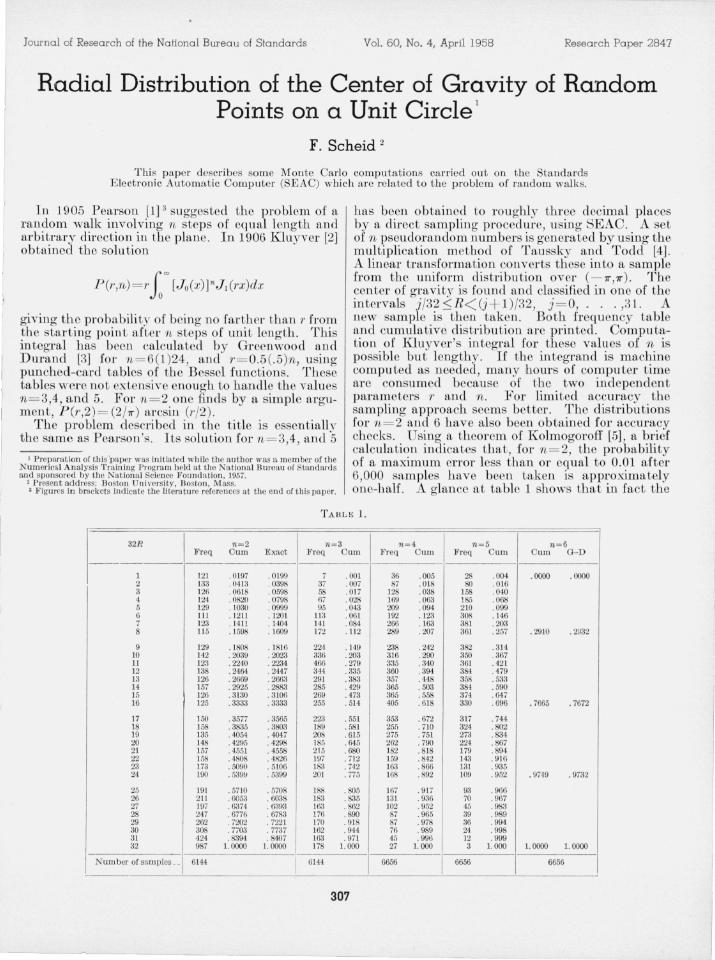
has been obtained to roughly three decimal places by a direct sampling procedure, u sing SEAC. A set of n pseudorandom numbers is genemted by using the multiplication method of Taussky and Todd [4] . A lineal' transformation converts these into a sample from the uniform distribution over (- 7T" ,7T"). The center of gravity is founa and classified in one of th e intervals j/32~R< (j+ l ) /32, j = O, . .. ,3 1. A new sample is then taken. Both frequ ency table and cumulative distribution are prin ted. Computation of Kluyver's integral for these valu es of n is possible but lengthy. If the integrand is mil,chin e computed as needed , many hours of computer time are consumed b ecau se of t·he two independent parameters r and n. For limited accuracy the ampling approach seems better. The dis tribu tions
for n = 2 and 6 have also b een obtained for accuracy checks. U ing a theorem of Kolmogoroff [5], a brief calculation indicates Lbat, for n = 2, tbe probability of a maximum error less than or equal to 0.01 after 6,000 samples have been taken is appro).'.imately on e-half. A glan ce at table 1 hows that in fa,ct the
32R n=2 n=3 n =4 n =5 n =6 Freq CUll Exact Frcq Cum Freq CllIn Freq Cum Cum G-D
-------1 121 .0197 .0199 7 . 001 36 . 005 28 . 004 . 0000 . 0000 2 133 . 04 13 . 0398 37 . 007 87 . 018 80 . 016 3 126 . 061 8 . 0598 58 . 017 128 . 038 158 . 040 4 124 . 0820 . 0798 117 . 028 169 . 063 185 .068 5 129 . 1030 . 0999 95 . 043 209 . 094 2 10 . 099 6 II I . 1211 . 1201 11 3 . 061 192 . 123 308 . 146 7 123 . 1411 . 1404 141 . 084 266 . 163 381 . 203 8 115 . 1598 . 1609 172 . 112 289 . 207 361 . 257 . 2910 .2932
9 129 . 1808 . 1816 224 .149 238 .242 382 .314 10 142 . 2039 .2023 336 .203 316 . 290 350 . 367 11 123 . 2240 . 2234 466 . 279 335 . 340 361 . 421 12 138 . 2464 . 2447 344 . :135 360 . 394 384 . 479 13 126 . 2669 .2663 291 . 383 :l5i . 448 358 . 533 14 157 . 2925 .2883 285 . 429 365 . 503 384 .590 15 126 . 3130 .3 106 269 . 473 365 .558 374 . 647 16 125 . 3333 . 3333 255 . 514 405 . 618 330 . 696 . 7665 .7672
17 150 .3577 . 3565 223 . 551 353 .672 317 . 744 18 158 . 3835 . 3803 189 . 581 25.1 . 710 324 . 802 19 135 .4054 . 4047 208 .615 275 . 751 273 . 834 20 148 . 4295 . 4298 185 . 64 5 262 . 790 224 .867 21 157 . 4.151 . 4558 215 . 680 182 .818 179 .894 22 158 . 4808 . 4826 197 . 712 159 .842 143 .916 23 173 .5090 .5 106 18,3 .7-12 163 . 866 131 . 935 24 190 .539!i .5399 201 . 775 168 .892 109 . 952 .9749 .9732
25 191 .5710 . 5708 188 .805 167 . 917 93 . 966 26 2 11 .6053 . 6038 183 . 835 131 . 936 70 . 967 27 197 .6374 .6.393 163 .862 102 . 952 45 . 983 28 247 .6776 .6783 176 .890 87 .965 39 .989 29 262 . 7202 . 7221 170 . 018 87 . 978 36 . 994 30 308 . 7703 .7737 162 . 944 76 . 989 24 . 998 31 424 . 8394 .8407 163 .971 45 .996 12 .999 32 987 1.0000 l. 0000 J 78 1.000 27 1.000 3 1.000 1.0000 1. 0000
N umber of sallP1es __ , 6144 I 6144 6656 6656 6656
- -
307
1
n=3 n=4 32R Frcq Cum FreCI Cum
L __ _________________ 4 2____________________ 10 3 __ __________________ 17 4_____ _______________ 19 5____ ________________ 48 6____________________ 45 7____ ________________ 76 8_____ _ _____________ 92
9 __ __ ________________ 107 10___ ________________ 160 lL __ ________________ 289 12___________________ 203 13___________________ 203 14___________________ 176 15_ ______ ____________ 177 16__ _________________ 185
17 ___________________ 170 18__ ________ _________ 172 19_ ________________ __ 176 20 ___________________ 196 2L __________________ 185 22 ___________________ 196 23 ___ ________________ 196 24- __ ________________ 172
25___________________ 184 26__ _________________ 224 21- __________________ 220 28 ___ ___ ________ _____ 236 29 ___ ___ _____________ 225 30 ___________________ 239 3L __________________ 239 32- __________________ 279
Number of samp1es __ 5120
. 001 9
. 003 29
. 006 50
. 010 59
. 019 71
. 028 88
. 043 69
. 061 109
. 082 133
. 113 126
. 169 151
. 209 191
. 249 221
. 283 231
. 318 232
. 354 287
. 387 248
. 421 237
. 455 235
. 493 235
. 529 215
. 568 191
. 606 229 • 639 210
. 675 205
. 719 183
. 762 188
. 808 183
. 852 167
. 899 152
. 946 120 1. 000 66
5120
. 002
.007
. 017
. 029
. 043
. 060
. 073
. 095
. 121
.145
.175
. 212
. 255
. 300
. 346
. 402
. 450
. 496
. 542
.588
. 630
.667
. 712
.753
• 793 . 829 . 866 . 901 . 934 . 964 .987
1.000
WASHINGTON, September 16,1957.
n=5 Freq Cum
7 . 002 17 . 006 21 . 011 40 . 021 61 . 036 72 . 053 99 . 077
113 .105
106 . . 131 120 . 160 142 . 195 149 . 231 ]77 . 274 167 . 215 227 . 371 217 . 424
242 234 237 207 208 178 179 168
148 156 117 97 77 65 34 14
4096
. 483
. 540
. 598
. 648
. 699
. 742
. 786
. 827
. 863
. 901
. 930
. 954
. 972
. 988
. 997 1.000
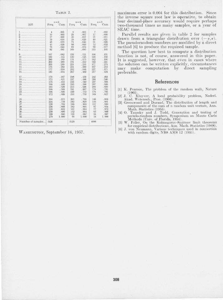
maximum error is 0.004 for this distribution. Since the Inverse square root law IS operative, to obtain four decimal-place accuracy would require perhaps two-thousand times as many samples, or a year of SEAC time .
Parallel results are given 111 table 2 for samples drawn from a triangular distribution over (- 71",71") . The pseudorandom numbers are modified by a direct method [6] to produce the required sample .
The question how best to compute a distribution function IS not, of course, answered 111 this paper . It is suggested, however, that even ll1 cases where the solution can be written explicitly, circumstances may make computation by direct sampling preferable .
References
[1] K . Pearson , The problem of the random walk, Jature (1905) .
[2] J . C. Kluyver, A local probability problem, Nederl. Akad. Wetensch., Proc. (1906) .
[3] Greenwood and Durand, The distributioll of length and components of the sum of n random unit vectors, Ann . Math. Statistics (1955) .
[4] O. Taussky and J. Todd, Generation and testing of pseudo-random numbers, Symposium on Monte Carlo Methods (Univ. of Florida, 1954).
[5] W. Feller, On the Kolmogorov-Smirnov limit theorems for empirical distributiollB, Anll . Math. Statistics (1948).
[6] J . von Neumann, Various techniques used in connection with random digits, NBS AMS 12 (1951) .
308