Random conformal weldings - MathSciDoc: An Archive for …archive.ymsc.tsinghua.edu.cn/pacm_download/117/6745... · · 2018-01-14The SLE curves come in two varieties: the radial

Acta Math., 207 (2011), 203–254DOI: 10.1007/s11511-012-0069-3c© 2011 by Institut Mittag-Leffler. All rights reserved

Random conformal weldings

by

Kari Astala

University of Helsinki

Helsinki, Finland

Peter Jones

Yale University

New Haven, CT, U.S.A.

Antti Kupiainen


Helsinki, Finland

Eero Saksman


Helsinki, Finland

1. Introduction

There has been great interest in conformally invariant random curves and fractals in theplane ever since it was realized that such geometric objects appear naturally in statisticalmechanics models at the critical temperature [13]. A major breakthrough in the fieldoccurred when O. Schramm [29] introduced the Schramm–Loewner evolution (SLE), astochastic process whose sample paths are conjectured (and in several cases proved) tobe the curves occurring in the physical models. We refer to [30] and [32] for a generaloverview and some recent work on SLE. The SLE curves come in two varieties: the radialone, where the curve joins a boundary point (say of the disc) to an interior point, andthe chordal case, where two boundary points are joined.

SLE describes a curve growing in time: the original curve of interest (say a clusterboundary in a spin system) is obtained as time tends to infinity. In this paper we give adifferent construction of random curves which is stationary, i.e. the probability measureon curves is directly defined without introducing an auxiliary time. We carry out thisconstruction for closed curves, a case that is not naturally covered by SLE.

Our construction is based on the idea of conformal welding. Consider a Jordancurve Γ bounding a simply connected region Ω in the plane. By the Riemann mappingtheorem, there are conformal maps f± mapping the unit disc D and its complement toΩ and its complement. The map f−1

+ f− extends continuously to the boundary T=∂Dof the disc, and defines a homeomorphism of the circle. Conformal welding is the inverse

K. A., A. K. and E. S. were supported by the Academy of Finland, P. J. by NSF, A. K. by ERCand K. A. by the EU-network CODY.

204 k. astala, p. jones, a. kupiainen and e. saksman

operation where, given a suitable homeomorphism of the circle, one constructs a Jordancurve on the plane (see §2). In fact, in our case the curve is determined up to a Mobiustransformation of the plane. Thus random curves (modulo Mobius transformations) canbe obtained from random homeomorphisms via welding.

In this paper we introduce a random scale invariant set of homeomorphisms hω: T!Tand construct the welding curves. The model considered here has been proposed by thesecond author. The construction depends on a real parameter β (the “inverse temper-ature”) and the maps are a.s. in ω Holder continuous for β<βc. For this range of βthe welding map will be a.s. well defined. For β>βc we expect the map hω not to becontinuous and no welding to exist. Our curves are closely related to SLE() for <4,see the footnote on page 205 and [31]. The case β=βc, presumably corresponding toSLE(4), is not covered by our analysis.

Since we are interested in random curves that are stochastically self-similar, it isnatural to take h with such properties. Our choice for h is constructed by starting withthe Gaussian random field X on the circle (see §3 for precise definitions) with covariance

EX(z)X(z′) =− log |z−z′|, (1)

where z, z′∈C have modulus 1. X is just the restriction of the 2-dimensional masslessfree field (Gaussian free field) on the circle. The exponential of βX gives rise to a randommeasure τ on the unit circle T, formally given by

“dτ = eβX(z) dz”. (2)

The proper definition involves a limiting process

τ(dz) = limε!0+

eβXε(z)

EeβXε(z)dz,

where Xε stands for a suitable regularization of X, see §3.3 below.Identifying the circle as T=R/Z=[0, 1), our random homeomorphism h: [0, 1)![0, 1)

is defined as

h(θ) =τ([0, θ))τ([0, 1))

for θ∈ [0, 1). (3)

The main result of this paper can then be summarized as follows.

For β2<2 and almost surely in ω, formula (3) defines a Holder continuous circlehomeomorphism, such that the welding problem has a solution Γ, where Γ is a Jordancurve bounding a domain Ω=f+(D) with a Holder continuous Riemann mapping f+. Fora given ω, the solution is unique up to a Mobius map of the plane. Moreover, the curveΓ is continuous in β∈[0,

√2 ).

random conformal weldings 205

We refer to §5 (Theorems 5.2 and 5.3) for the exact statement of the main result.With minor changes our method generalizes to the situation where(1) the random

homeomorphism φ is replaced by φ+φ−1− , where φ+ and φ− are random circle homeo-

morphisms having the same distribution as φ with parameters β+ and β−, respectively,i.e. formally

dφ±∼ eβ±X(z)dz.

In the case where φ± are independent, we have the following result.

For every pair β+, β−<√

2 and almost surely in ω, the welding problem for thehomeomorphism φ+φ

−1− has a solution Γ=Γβ+,β− , where Γβ+,β− is a Jordan curve

bounding the domains Ω+=f+(D) and Ω−=f−(C\D), with Holder continuous Riemannmappings f±. For a given ω, the solution is unique up to a Mobius map of the plane andthe curves Γβ+,β− are continous in β+ and β−.

Apart from connection to SLE, the weldings constructed in this paper should be ofinterest to complex analysts as they form a natural family that degenerates as β"

√2.

It would be of great interest to understand the critical case β=√

2 as well as the lowtemperature “spin glass phase” β>

√2. It would also be of interest to understand the

connection of our weldings to those arising from stochastic flows [2]. In [2] Holder con-tinuous homeomorphisms are considered, but the boundary behavior of the welding andhence its existence and uniqueness are left open.

In writing the paper we have tried to be generous in providing details on both thefunction-theoretic and the stochastics notions and tools needed, in order to serve readerswith varied backgrounds. The structure of the paper is as follows. §2 contains backgroundmaterial on conformal welding and the geometric-analysis tools we need later on. To bemore specific, §2 recalls the notion of conformal welding and explains how the weldingproblem is reduced to the study of the Beltrami equation. Also we recall a useful methoddue to Lehto [23] to prove the existence of a solution for a class of non-uniformly ellipticBeltrami equations, and a theorem by Jones and Smirnov [18] that will be used to verifythe uniqueness of our welding. Finally we recall the Beurling–Ahlfors extension of circlehomeomorphisms to the unit disc. For our purposes we need to estimate carefully thedependence of the dilatation of the extension in a Whitney cube by just using smallamount of information of the homeomorphism on a ‘shadow’ of the cube.

In §3 we introduce the 1-dimensional trace of the Gaussian free field and recall someknown properties of its exponential that we will use to define and study the random

(1) Heuristic arguments from Liouville quantum gravity suggest [11], [15] that there might be a

more precise relation between SLE and the welding of the homeomorphism φ−1+ φ−, which we do not

consider here as it would require considerable changes in our argument.


circle homeomorphism. §4 is the technical core of the paper as it contains the mainprobabilistic estimates we need to control the random dilatation of the extension map.Finally, in §5 things are put together and the a.s. existence and uniqueness of the weldingmap is proven.

Let us conclude by a remark on notation. We denote by c and C generic constantswhich may vary between estimates. When the constants depend on parameters such asβ we denote this by C(β).

Acknowledgements. We thank M. Bauer, D. Bernard, I. Binder, M. Nikula, S. Ro-hde, S. Smirnov and W. Werner for useful discussions.

Note added in proof. After the manuscript was sent to publication, the works [3]and [31] have appeared. The paper [3] by Airault, Malliavin and Thalmayer continuesthe work on the welding of stochastic flows initiated in [2]. Sheffield’s preprint [31]contains, among other things, confirmation for the close relation between welding of thehomeomorphism φ−1

+ φ− and SLE, see the footnote on page 205.

2. Conformal welding

In this section we recall for the general readers benefit basic notions and results fromgeometric analysis that are needed in our work. In particular, we recall the notion ofconformal welding, Lehto’s method for solving the Beltrami equations, the uniquenessresult for weldings due to Jones and Smirnov, and the last subsection contains estimatesfor the Beurling–Ahlfors extension tailored for our needs.

2.1. Welding and Beltrami equation

One of the main methods for constructing conformally invariant families of (Jordan)curves comes from the theory of conformal welding. Put briefly, in this method weglue the unit disc D=z∈C:|z|<1 and the exterior disc D∞=z∈C:|z|>1 along ahomeomorphism φ: T!T, by the identification

x∼ y, when x∈T = ∂D and y=φ(x)∈T = ∂D∞.

The problem of welding is to give a natural complex structure to this topological sphere.Uniformizing the complex structure then gives us the curve, the image of the unit circle.

More concretely, given a Jordan curve Γ⊂C, let

f+: D!Ω+ and f−: D∞!Ω−


be a choice of Riemann mappings onto the components of the complement C\Γ=Ω+∪Ω−.By Caratheodory’s theorem, f− and f+ both extend continuously to ∂D=∂D∞, and thus

φ= f−1+ f− (4)

is a homeomorphism of T. In the welding problem we are asked to invert this process;given a homeomorphism φ: T!T we are to find a Jordan curve Γ and conformal mappingsf± onto the complementary domains Ω± so that (4) holds.

It is clear that the welding problem, when solvable, has natural conformal invarianceattached to it; any image of the curve Γ under a Mobius transformation of C is equally awelding curve. Similarly, if φ: T!T admits a welding, then so do all its compositions withMobius transformations of the disc. Note, however, that not all circle homeomorphismsadmit a welding, for examples see [26] and [34].

The most powerful tool in solving the welding problem is given by the Beltramidifferential equation, defined in a domain Ω by

∂f

∂z=µ(z)

∂f

∂zfor a.e. z ∈Ω, (5)

where we look for homeomorphic solutions f∈W 1,1loc (Ω). Here (5) is an elliptic system

whenever |µ(z)|<1 almost everywhere, and uniformly elliptic if ‖µ‖∞<1.In the uniformly elliptic case, homeomorphic solutions to (5) exist for every co-

efficient with ‖µ‖∞<1, and they are unique up to post-composing with a conformalmapping [5, p. 179]. In fact, it is this uniqueness property that gives us a way to producethe welding. To see this, suppose first that

φ= f |T, (6)

where f∈W 1,2loc (D; D)∩C(D) is a homeomorphic solution to (5) in the disc D. Find then

a homeomorphic solution to the auxiliary equation

∂F

∂z=χD(z)µ(z)

∂F

∂zfor a.e. z ∈C. (7)

Now Γ=F (T) is a Jordan curve. Moreover, as ∂zF=0 for |z|>1, we can set f− :=F |D∞and Ω− :=F (D∞) to define a conformal mapping

f−: D∞!Ω−.

On the other hand, since both f and F solve the equation (5) in the unit disc D, byuniqueness of the solutions we have

F (z) = f+f(z), z ∈D, (8)


for some conformal mapping f+: D=f(D)!Ω+ :=F (D). Finally, on the unit circle,

φ(z) = f |T(z) = f−1+ f−(z), z ∈T. (9)

Thus we have found a solution to the welding problem, under the assumption (6). Thatthe welding curve Γ is unique up to a Mobius transformation of C follows from [5,Theorem 5.10.1]; see also Corollary 2.5 below.

To complete this circle of ideas, we need to identify the homeomorphisms φ: T!Tthat admit the representation (5), (6) with uniformly elliptic µ in (5). It turns out[5, Lemma 3.11.3 and Theorem 5.8.1] that such φ’s are precisely the quasisymmetricmappings of T, mappings that satisfy

K(φ) := sups,t∈R

|φ(e2πi(s+t))−φ(e2πis)||φ(e2πi(s−t))−φ(e2πis)|

<∞. (10)

2.2. Existence in the degenerate case: the Lehto condition

The previous subsection describes an obvious model for constructing random Jordancurves, by first finding random homeomorphisms of the circle and then solving for eachof them the associated welding problem. In the present work, however, we are faced withthe obstruction that circle homeomorphisms with the exponentiated Gaussian free fieldas derivative almost surely do not satisfy the quasisymmetry assumption (10). Thuswe are forced outside the uniformly elliptic partial differential equations and need tostudy (5) with degenerate coefficients with only |µ(z)|<1 almost everywhere. We areeven outside the much studied class of maps of exponentially integrable distortion, see[5, §20.4.] In such generality, however, the homeomorphic solutions to (5) may fail toexist, or the crucial uniqueness properties of (5) may similarly fail.

In his important work [23], Lehto gave a very general condition in the degeneratesetting for the existence of homeomorphic solutions to (5). To recall his result, assumewe are given the complex dilatation µ=µ(z), and write then

K(z) =1+|µ(z)|1−|µ(z)|

, z ∈Ω,

for the associated distortion function. Note that K(z) is bounded precisely when theequation (5) is uniformly elliptic, i.e. ‖µ‖∞<1. Thus the question is how strongly K(z)can grow for the basic properties of (5) still to remain true. In order to state Lehto’scondition we fix some notation. For given z∈C and radii 06r<R<∞, let us denote thecorresponding annulus by

A(z, r, R) := w∈C : r < |w−z|<R.


In the Lehto approach, one needs to control the conformal moduli of image annuli in asuitable way. This is done by introducing, for any annulus A(w, r,R) and for the givendistortion function K, the following quantity, which we call the Lehto integral :

L(z, r, R) :=LK(z, r, R) :=∫ R

r

1∫ 2π

0K(z+%eiθ) dθ

d%

%. (11)

For the following formulation of Lehto’s theorem see [5, p. 584].

Theorem 2.1. Suppose µ is measurable and compactly supported with |µ(z)|<1 foralmost every z∈C. Assume that the distortion function

K(z) =1+|µ(z)|1−|µ(z)|

is locally integrable, that isK ∈L1

loc(C), (12)

and that for some R0>0 the Lehto integral satisfies

LK(z, 0, R0) =∞ for all z ∈C. (13)

Then the Beltrami equation

∂f

∂z(z) =µ(z)

∂f

∂z(z) for a.e. z ∈C (14)

admits a homeomorphic W 1,1loc -solution f : C!C.

As a consequence, the welding extends beyond the class of quasisymmetric functions.

Corollary 2.2. Suppose that φ: T!T extends to a homeomorphism f : C!C sat-isfying (12)–(14) together with the condition

K(z)∈L∞loc(D). (15)

Then φ admits a welding : there are a Jordan curve Γ⊂C and conformal mappingsf± onto the complementary domains of Γ such that

φ(z) = f−1+ f−(z), z ∈T.

Proof. Given the extension f : C!C, let us again look at the auxiliary equation

∂F

∂z=χD(z)µ(z)

∂F

∂zfor a.e. z ∈C. (16)


Since Lehto’s condition holds as well for the new distortion function

K(z) =1+|χD(z)µ(z)|1−|χD(z)µ(z)|

,

we see from Theorem 2.1 that the auxiliary equation (16) admits a homeomorphic solutionF : C!C. Arguing as in (6)–(9), it will then be sufficient to show that

F (z) = f+f(z), z ∈D,

where f+ is conformal in D. But this is a local question; every point z∈D has a neigh-borhood where K(z) is uniformly bounded, by (15). In such a neighborhood the usualuniqueness results to solutions of (5) apply; see [5, p. 179]. Thus f+ is holomorphic, andas a homeomorphism it is conformal. This proves the claim.

Consequently, in the study of random circle homeomorphisms φ=φω, a key step forthe conformal welding of φω will be to show that almost surely each such mapping admitsa homeomorphic extension to C, where the distortion function satisfies a condition suchas (13). In our setting where the derivative of φ is given by the exponentiated trace ofa Gaussian free field, the extension procedure is described in §2.4 and the appropriateestimates it requires are proven in §4.

Actually, in §5, when proving our main theorem, we need to present a variant ofLehto’s argument where it will be enough to estimate the Lehto integral only at a suitablecountable set of points z∈T. We also utilize there the fact that the extension of ourrandom circle homeomorphism φ satisfies (15). In verifying the Holder continuity of theensuing map, we shall apply a useful estimate (Lemma 2.3 below) that estimates thegeometric distortion of an annulus under a quasiconformal map.

Given a bounded (topological) annulus A⊂C, with E being the bounded componentof C\A, we denote by DO(A):=diam(A) the outer diameter, and by DI(A):=diam(E)the inner diameter of A.

Lemma 2.3. Let f be a quasiconformal mapping on the annulus A(w, r,R), withdistortion function Kf . It then holds that

DO(f(A(w, r,R)))DI(f(A(w, r,R)))

>116e2π

2LKf(w,r,R).

Proof. Recall first that for a rigid annulus A=A(w, r,R), we define its conformalmodulus by

mod(A) = 2π logR

r,


while for any topological annulus A, one sets

mod(A) =mod(g(A)),

where g is a conformal map of A onto a rigid annulus. Then we have [5, Corollary 20.9.2]the following basic estimate for the modulus of the image annulus in terms of the Lehtointegrals:

mod(f(A(w, r,R)))> 2πLKf(w, r,R). (17)

On the other hand, by combining [35, Lemma 7.38 and Corollary 7.39] and [4, Exer-cise 5.68 (16)] we obtain for any bounded topological annulus A⊂C,

116eπmod(A) 6

DO(A)DI(A)

.

Put together, the desired estimate follows.

2.3. Uniqueness of the welding

An important issue of the welding is its uniqueness, that the curve Γ is unique up to com-posing with a Mobius transformation of C. As the above argument indicates, this is es-sentially equivalent to the uniqueness of solutions to the appropriate Beltrami equations,up to a Mobius transformation. However, in general the assumptions of Theorem 2.1alone are much too weak to imply this.

In fact, in our case the uniqueness of solutions to the Beltrami equation (16) isequivalent to the conformal removability of the curve F (T). Recall that a compact setB⊂C is conformally removable if every homeomorphism of C which is conformal off B

is conformal in the whole sphere, and hence a Mobius transformation.It follows easily that e.g. images of circles under quasiconformal mappings, i.e.

homeomorphisms satisfying (5), with ‖µ‖∞<1, are conformally removable, while Jor-dan curves of positive area are never conformally removable.

For general curves the removability is a deep problem; no characterization of confor-mally removable Jordan curves is known to this date. What saves us in the present workis that we have the remarkable result of Jones and Smirnov in [18] available. We will notneed their result in its full generality, as the following special case will be sufficient forour purposes.

Theorem 2.4. (Jones–Smirnov [18]) Let Ω⊂C be a simply connected domain suchthat the Riemann mapping ψ: D!Ω is α-Holder continuous for some α>0.

Then the boundary ∂Ω is conformally removable.

Adapting this result to our setting, we obtain the following result.


Corollary 2.5. Suppose that φ: T!T is a homeomorphism that admits a welding

φ(z) = f−1+ f−(z), z ∈T,

where f± are conformal mappings of D and D∞, respectively, onto complementary Jordandomains Ω±.

Assume that f− (or f+) is α-Holder continuous on the boundary ∂D∞=T. Thenthe welding is unique: any other welding pair (g+, g−) of φ is of the form

g± =Φf±,

where Φ: C!C is a Mobius transformation.

Proof. Suppose we have Riemann mappings g± onto complementary Jordan domainssuch that

g−1+ g−(z) =φ(z) = f−1

+ f−(z), z ∈T.

Then the formula

Ψ(z) =g+f

−1+ (z), if z ∈ f+(D),

g−f−1− (z), if z ∈ f−(D∞)

defines a homeomorphism of C which is conformal outside Γ=f±(T). From the Jones–Smirnov theorem we see that Ψ extends conformally to the entire sphere, and thus it isa Mobius transformation.

As we shall see in Theorem 5.1, for circle homeomorphisms φ with the exponentiatedGaussian free field as derivative, the solutions F to the auxiliary equation (16) willbe Holder continuous almost surely. Then f−=F |D∞ is a Riemann mapping onto acomplementary component of the welding curve of φ=φω. It follows that almost surelyφ=φω admits a welding curve Γ=Γω which is unique, up to composing with a Mobiustransformation.

2.4. Extension of the homeomorphism

In this section we discuss in detail suitable methods for extending homeomorphismsφ: T!T to the unit disc; by reflecting across T, the map then extends to C. Extensions ofhomeomorphisms h: R!R of the real line are convenient to describe, and it is not difficultto find constructions that sufficiently well respect the conformally invariant features of h.Given a homeomorphism φ: T!T on the circle, we hence represent it in the form

φ(e2πix) = e2πih(x), (18)


where h: R!R is a homeomorphism of the line with h(x+1)=h(x)+1. We may assumethat φ(1)=1, with h(0)=0.

We will now extend the 1-periodic mapping h to the upper (or lower) half-plane sothat it becomes the identity map at large height. Then a conjugation to a mapping ofthe disc is easily done. For the extension we use the classical Beurling–Ahlfors extension[10] modified suitably far away from the real axis.

Thus, given a homeomorphism h: R!R such that

h(x+1) =h(x)+1, x∈R, with h(0)= 0, (19)

we define our extension F as follows. For 0<y<1 let

F (x+iy) =12

∫ 1

0

(h(x+ty)+h(x−ty)) dt+i∫ 1

0

(h(x+ty)−h(x−ty)) dt. (20)

Then F=h on the real axis, and F is a continuously differentiable homeomorphism.Moreover, by (19), it follows that for y=1,

F (x+i) =x+i+c0,

where c0=∫ 1

0h(t) dt− 1

2∈[− 1

2 ,12

]. Thus, for 16y62, we set

F (z) = z+(2−y)c0, (21)

and finally have an extension of h with the extra properties

F (z)≡ z when y=Imm(z) > 2, (22)

F (z+k) =F (z)+k, k∈Z. (23)

The original circle mapping admits a natural extension to the disc,

Ψ(z) = exp(

2πiF(

log z2πi

)), z ∈D. (24)

From (18) and (23) we see that this is a well-defined homeomorphism of the disc withΨ|T=φ and Ψ(z)≡z for |z|6e−4π. The distortion properties are not altered under thislocally conformal change of variables,

K(z,Ψ)=K(w,F ), z= e2πiw, w∈H, (25)

so we will reduce all distortion estimates for Ψ to the corresponding ones for F . Since Fis conformal for y>2, it suffices to restrict the analysis to the strip

S= R×[0, 2]. (26)


To estimate K(w,F ) we introduce some notation. Let

Dn = [k2−n, (k+1)2−n] : k∈Z

be the set of all dyadic intervals of length 2−n and write

D= Dn :n> 0.

Consider the measureτ([a, b])=h(b)−h(a).

For a pair of intervals J=J1, J2 let us introduce the following quantity

δτ (J) =τ(J1)τ(J2)

+τ(J2)τ(J1)

. (27)

If J1 and J2 are the two halves of an interval I, then δτ (J) measures the local doublingproperties of the measure τ . In such a case we define δτ (I)=δτ (J). In particular, (10)holds for the circle homeomorphism φ(e2πix)=e2πih(x) if and only if the quantities δτ (I)are uniformly bounded, for all (not necessarily dyadic) intervals I.

The local distortion of the extension F will be controlled by sums of the expressionsδτ (J) in the appropriate scale. For this, let us pave the strip S by Whitney cubes CII∈Ddefined by

CI = (x, y) :x∈ I and 2−n−1 6 y6 2−n

for I∈Dn, n>0, and CI=I×[12 , 2]

for I∈D0. Given an I∈Dn let j(I) be the union of Iand its neighbors in Dn and

J (I) := J=(J1, J2) :J1, J2 ∈Dn+5 and J1, J2⊂ j(I). (28)

We then defineKτ (I) :=

∑J∈J (I)

δτ (J). (29)

With these notions we have the basic geometric estimate for the distortion function,in terms of the boundary homeomorphism.

Theorem 2.6. Let h: R!R be a 1-periodic homeomorphism and let F : H!H be itsextension. Then, for each I∈D,

supz∈CI

K(z, F ) 6C0Kτ (I), (30)

with a universal constant C0.


Proof. The distortion properties of the Beurling–Ahlfors extension are well studiedin the existing litterature, but none of these works gives directly Theorem 2.6, as themain point for us is the linear dependence on the local distortion Kτ (I). The mostelementary extension operator is due to Jerison and Kenig [17] (see also [5, §5.8]), butfor this extension the linear dependence fails.

For the reader’s convenience we sketch a proof of the theorem. We will modify theapproach of Reed [27], and start with a simple lemma.

Lemma 2.7. For each dyadic interval

I = [k2−n, (k+1)2−n],

with left half I1=[k2−n,

(k+ 1

2

)2−n

]and right half I2=I\I1, we have

11+δτ (I)

|τ(I)|6 |τ(Ij)|6δτ (I)

1+δτ (I)|τ(I)|,

j=1, 2, with1|I|

∫I

(h(t)−h(k2−n)) dt6 3δτ (I)1+3δτ (I)

|τ(I)|

and1|I|

∫I

(h((k+1)2−n)−h(t)) dt6 3δτ (I)1+3δτ (I)

|τ(I)|.

Proof. The definition of δτ (I) gives the first estimate. As h(t)6h((k+ 1

2

)2−n

)on

the left half and h(t)6h((k+1)2−n) on the right half of I, we have

1|I|

∫I

(h(t)−h(k2−n)) dt6(

12

δτ (I)1+δτ (I)

+12

)|τ(I)|6 3δτ (I)

1+3δτ (I)|τ(I)|.

The last estimate follows similarly.

To continue with the proof of Theorem 2.6, the pointwise distortion of the extensionF is easy to calculate explicitly, and we obtain [10], [27] the following estimate, sharp upto a multiplicative constant,

K(x+iy, F ) 6

(α(x, y)β(x, y)

+β(x, y)α(x, y)

)[α(x, y)α(x, y)

+β(x, y)β(x, y)

]−1

, (31)

whereα(x, y) =h(x+y)−h(x), β(x, y) =h(x)−h(x−y)

and

α(x, y) =h(x+y)− 1y

∫ x+y

x

h(t) dt, β(x, y) =1y

∫ x

x−yh(t) dt−h(x−y).


Now the argument of Reed [27, pp. 461–464], combined with Lemma 2.7 and its estimates,precisely shows that K(x+iy, F )624 max δτ (I), where I runs over the intervals withendpoints contained in the set

x, x± 14y, x±

12y, x±y

. (32)

Thus, for example, if we fix k∈Z and n∈N, we get for the corner point z=k2−n+i2−n

of the Whitney cube CI the estimate

K(k2−n+i2−n, F ) 6 24∑J

δτ (J), J=(J1, J2), J1, J2 ∈Dn+3, (33)

where J1, J2⊂j(I) as above. For a general point z=x+iy∈CI , we have to take a fewmore generations of dyadic intervals. Here

[x, x+ 1

4y]

has length at least 2−n−3. On theother hand, for any (non-dyadic) interval I with 2−m6|I|<2−m+1, one observes that itcontains a dyadic interval of length 2−m−1 and is contained inside a union of at mostthree dyadic intervals of length 2−m. By this manner, one estimates

δτ (I) 6∑J

δτ (J), where J=(J1, J2), Jk ∈Dm+2 and Jk∩I 6= ∅, k=1, 2.

Choosing the endpoints of I from the set in (32) then gives the bound (30). Note thatthe estimates hold also for n=0, since by (21) we have K(z, F )6 5

4 whenever y>1. Hencethe proof of Theorem 2.6 is complete.

3. Exponential of GFF and random homeomorphisms of T

3.1. Trace of the Gaussian free field

Let us recall that the 2-dimensional Gaussian free field (in other words, the massless freefield) Y in the plane has the covariance

EY (x)Y (x′) = log1

|x−x′|, x, x′ ∈R2.

Actually, the definition of this field in the whole plane has to be done carefully, becauseof the blowup of the logarithm at infinity. However, the definition of the trace X :=Y |Ton the unit circle T avoids this problem, since it is formally obtained by requiring (in theconvenient complex notation) that

EX(z)X(z′) = log1

|z−z′|, z, z′ ∈T. (34)


The above definition needs to be made precise. In order to serve also readers with lessbackground in non-smooth stochastic fields, let us first recall the definition of Gaussianrandom variables with values in the space of distributions D′(T). An element in F∈D′(T)is real-valued if it takes real values on real-valued test functions. Identifying T with [0, 1),a real-valued F may be written as

F = a0+∞∑n=1

(an cos 2πnt+bn sin 2πnt),

with real coefficients satisfying |an|, |bn|=O(na) for some a∈R. Conversely, every suchFourier series converges in D′(T).

Let (Ω,F ,P) stand for a probability space. A map X: Ω!D′(T) is a (real-valued)centered D′(T)-valued Gaussian if for every (real-valued) ψ∈C∞0 (T) the map

ω 7−! 〈X(ω), ψ〉

is a centered Gaussian on Ω. Here 〈· , ·〉 refers to the standard distributional duality.Alternatively, one may define such a random variable by requiring that a.s.

X(ω) =A0(ω)+∞∑n=1

(AN (ω) cos 2πnt+Bn(ω) sin 2πnt),

where An and Bn are centered Gaussians satisfying EA2n,EB2

n=O(na) for some a∈R.The random variable X is stationary if and only if the coefficients A0, A1, ..., B1, B2, ...

are independent.Due to Gaussianity, the distribution of X is uniquely determined by the knowledge

of the covariance operator CX :C∞(T)!D′(T), where

〈CXψ1, ψ2〉 := E〈X(ω), ψ1〉〈X(ω), ψ2〉.

In case the covariance operator has an integral kernel, we use the same symbol for thekernel, and in this case for almost every z∈T one has

(CXψ)(z) =∫

TCX(z, w)ψ(w)m(dw),

where m stands for the normalized Lebesgue measure on T. Most of the above definitionsand statements carry over directly on S ′(R)-valued random variables, but the aboveknowledge is enough for our purposes.

The exact definition of (34) is understood in the above sense.


Definition 3.1. The trace X of the 2-dimensional GFF (Gaussian free field) on T isa centered D′(T)-valued Gaussian random variable such that its covariance operator hasthe integral kernel

CX(z, z′) = log1

|z−z′|, z, z′ ∈T.

Observe that in the identification T=[0, 1) the covariance of X takes the form

CX(t, u) = log1

2 sinπ|t−u|for t, u∈ [0, 1). (35)

The existence of such a field is most easily established by writing down the Fourierexpansion:

X =∞∑n=1

1√n

(An cos 2πnt+Bn sin 2πnt), t∈ [0, 1), (36)

where all the coefficients An, Bn∼N(0, 1), n>1, are independent standard Gaussians.Writing X as

∞∑n=1

1√n

(αnzn+αnzn)

with |z|=1 and α= 12 (A+iB), it is readily checked that it has the stated covariance.

What makes the trace X of the 2-dimensional GFF particularly natural for thecircle homeomorphisms is its invariance properties, that X is Mobius invariant moduloconstants. To see this, note that the covariance C(z, z′)=log(1/|z−z′|) satisfies thetransformation rule

C(g(z), g(z′))=C(z, z′)+A(z)+B(z′),

where A (resp. B) is independent of z′ (resp. z), whence the last two terms vanish inintegration against mean-zero test-functions.

It is well known that, with probability 1, X(ω) is not an element in L1(T) (or ameasure on T), but it just barely fails to be a function-valued field. Namely, if ε>0and one considers the ε-smoothened field (1−∆)−εX, one computes that this field has aHolder-continuous covariance, whence its realization belongs to C(T) almost surely. Thisfollows from the following fundamental result of Dudley which we will use repeatedly.

Theorem 3.2. Let (Yt)t∈T be a centered Gaussian field indexed by the set T , whereT is a compact metric space with distance d. Define the (pseudo)distance d′ on T bysetting d′(t1, t2)=(E|Yt1−Yt2 |2)1/2 for t1, t2∈T . Assume that d′:T×T!R is continu-ous. For δ>0 denote by N(δ) the minimal number of balls of radius δ in the d′-metricneeded to cover T . If ∫ 1

0

√logN(δ) dδ <∞, (37)

then Y has a continuous version, i.e. almost surely the map T3t 7!Yt is continuous.


For a proof we refer to [1, Theorem 1.3.5] or [19, Chapter 15, Theorem 4]. The secondresult we will need is an inequality due to C. Borell and, independently, to B. Tsirelson,I. Ibragimov and V. Sudakov. According to the inequality, the tail of the supremum isdominated by a Gaussian tail:

P(

supt∈T

|Yt|>u)

6AeBu−u2/2σ2

T , (38)

where σT :=maxt∈T (EY 2t )1/2, and the constants A and B depend on (T, d′), see [1, §2.1].

We shall also need an explicit quantitative version of this inequality in the special casewhere T is an interval.

Lemma 3.3. Let T=[x0, x0+`], and suppose that the covariance is Lipschitz contin-uous with constant L, i.e. E|Yt−Yt′ |26L|t−t′| for t, t′∈T . Assume also that Yt0≡0 fora t0∈T . Then

P(

supt∈T

|Yt|>√L`u

)6 c(1+u)e−u

2/2,

where c is a universal constant.

Proof. The result is essentially due to Samorodnitsky [28] and Talagrand [33]. Itis a direct consequence of [1, Theorem 4.1.2], since after scaling it is possible to assumethat L=1=`, and then σT61 and N(ε)61/ε2.

3.2. White noise expansion

The Fourier series expansion (36) is often not the most suitable representation of X forexplicit calculations. Instead, we shall apply a representation that uses white noise inthe upper half-plane, due to Bacry and Muzy [6]. The white noise representation is veryconvenient, since it allows one to consider correlation between different scales both on thestochastic side and on T in a flexible and geometrically transparent manner. Moreover,as we define the exponential of the field X in the next subsection we are then able torefer to known results in [6] and elsewhere.

To commence with, let λ stand for the hyperbolic area measure in the upper half-plane H,

λ(dx dy) =dx dy

y2.

Denote by w a white noise in H with respect to the measure λ. More precisely, w is acentered Gaussian process indexed by Borel sets A∈Bf (H), where

Bf (H) :=A⊂H Borel :λ(A)<∞ and sup

(x,y),(x′,y′)∈A|x′−x|<∞

,


H+x

V +x

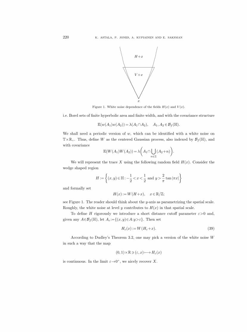
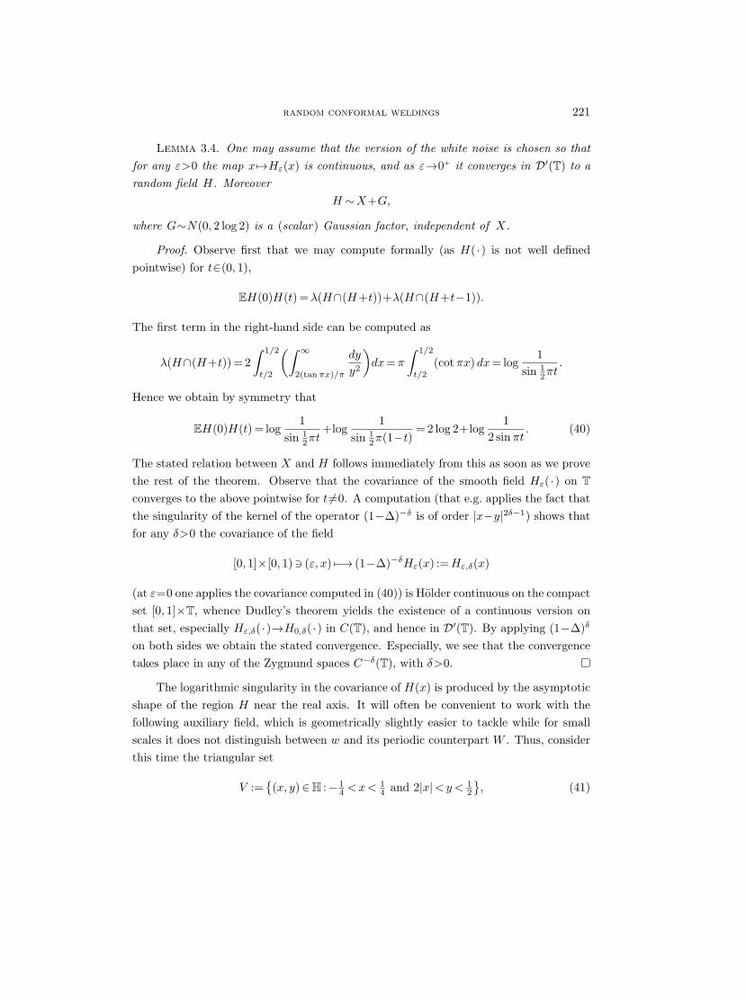
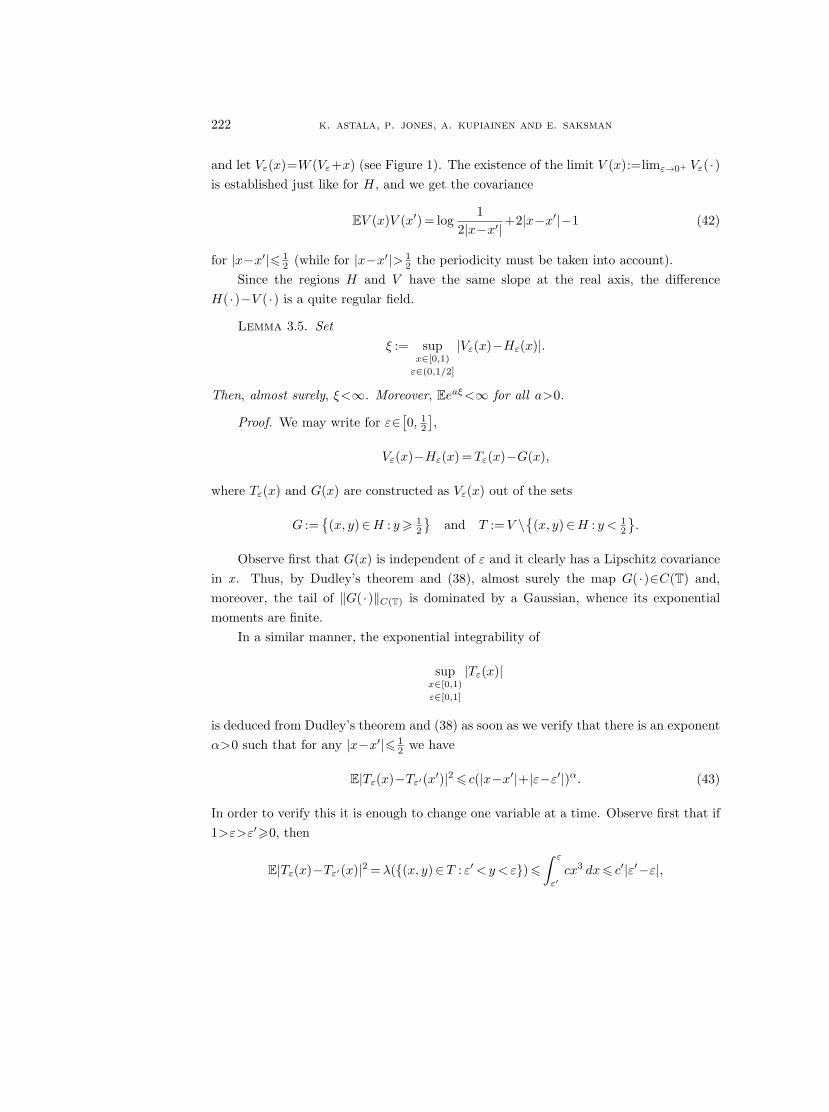
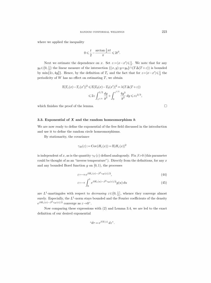
x

Figure 1. White noise dependence of the fields H(x) and V (x).

i.e. Borel sets of finite hyperbolic area and finite width, and with the covariance structure

E(w(A1)w(A2))=λ(A1∩A2), A1, A2 ∈Bf (H).

We shall need a periodic version of w, which can be identified with a white noise onT×R+. Thus, define W as the centered Gaussian process, also indexed by Bf (H), andwith covariance

E(W (A1)W (A2))=λ

(A1∩

⋃n∈Z

(A2+n)).

We will represent the trace X using the following random field H(x). Consider thewedge shaped region

H :=

(x, y)∈H :−12<x<

12

and y >2π

tan |πx|

and formally setH(x) :=W (H+x), x∈R/Z;

see Figure 1. The reader should think about the y-axis as parametrizing the spatial scale.Roughly, the white noise at level y contributes to H(x) in that spatial scale.

To define H rigorously we introduce a short distance cutoff parameter ε>0 and,given any A∈Bf (H), let Aε :=(x, y)∈A:y>ε. Then set

Hε(x) :=W (Hε+x). (39)

According to Dudley’s Theorem 3.2, one may pick a version of the white noise Win such a way that the map

(0, 1)×R3 (ε, x) 7−!Hε(x)

is continuous. In the limit ε!0+, we nicely recover X.


Lemma 3.4. One may assume that the version of the white noise is chosen so thatfor any ε>0 the map x 7!Hε(x) is continuous, and as ε!0+ it converges in D′(T) to arandom field H. Moreover

H ∼X+G,

where G∼N(0, 2 log 2) is a (scalar) Gaussian factor, independent of X.

Proof. Observe first that we may compute formally (as H( ·) is not well definedpointwise) for t∈(0, 1),

EH(0)H(t) =λ(H∩(H+t))+λ(H∩(H+t−1)).

The first term in the right-hand side can be computed as

λ(H∩(H+t))= 2∫ 1/2

t/2

(∫ ∞

2(tanπx)/π

dy

y2

)dx=π

∫ 1/2

t/2

(cotπx) dx= log1

sin 12πt

.

Hence we obtain by symmetry that

EH(0)H(t) = log1

sin 12πt

+log1

sin 12π(1−t)

= 2 log 2+log1

2 sinπt. (40)

The stated relation between X and H follows immediately from this as soon as we provethe rest of the theorem. Observe that the covariance of the smooth field Hε( ·) on Tconverges to the above pointwise for t 6=0. A computation (that e.g. applies the fact thatthe singularity of the kernel of the operator (1−∆)−δ is of order |x−y|2δ−1) shows thatfor any δ>0 the covariance of the field

[0, 1]×[0, 1)3 (ε, x) 7−! (1−∆)−δHε(x) :=Hε,δ(x)

(at ε=0 one applies the covariance computed in (40)) is Holder continuous on the compactset [0, 1]×T, whence Dudley’s theorem yields the existence of a continuous version onthat set, especially Hε,δ( ·)!H0,δ( ·) in C(T), and hence in D′(T). By applying (1−∆)δ

on both sides we obtain the stated convergence. Especially, we see that the convergencetakes place in any of the Zygmund spaces C−δ(T), with δ>0.

The logarithmic singularity in the covariance of H(x) is produced by the asymptoticshape of the region H near the real axis. It will often be convenient to work with thefollowing auxiliary field, which is geometrically slightly easier to tackle while for smallscales it does not distinguish between w and its periodic counterpart W . Thus, considerthis time the triangular set

V :=(x, y)∈H :− 1

4 <x<14 and 2|x|<y< 1

2

, (41)


and let Vε(x)=W (Vε+x) (see Figure 1). The existence of the limit V (x):=limε!0+ Vε( ·)is established just like for H, and we get the covariance

EV (x)V (x′) = log1

2|x−x′|+2|x−x′|−1 (42)

for |x−x′|6 12 (while for |x−x′|> 1

2 the periodicity must be taken into account).Since the regions H and V have the same slope at the real axis, the difference

H( ·)−V ( ·) is a quite regular field.

Lemma 3.5. Setξ := sup

x∈[0,1)

ε∈(0,1/2]

|Vε(x)−Hε(x)|.

Then, almost surely, ξ<∞. Moreover, Eeaξ<∞ for all a>0.

Proof. We may write for ε∈[0, 1

2

],

Vε(x)−Hε(x) =Tε(x)−G(x),

where Tε(x) and G(x) are constructed as Vε(x) out of the sets

G :=(x, y)∈H : y> 1

2

and T :=V \

(x, y)∈H : y < 1

2

.

Observe first that G(x) is independent of ε and it clearly has a Lipschitz covariancein x. Thus, by Dudley’s theorem and (38), almost surely the map G( ·)∈C(T) and,moreover, the tail of ‖G( ·)‖C(T) is dominated by a Gaussian, whence its exponentialmoments are finite.

In a similar manner, the exponential integrability of

supx∈[0,1)

ε∈[0,1]

|Tε(x)|

is deduced from Dudley’s theorem and (38) as soon as we verify that there is an exponentα>0 such that for any |x−x′|6 1

2 we have

E|Tε(x)−Tε′(x′)|2 6 c(|x−x′|+|ε−ε′|)α. (43)

In order to verify this it is enough to change one variable at a time. Observe first that if1>ε>ε′>0, then

E|Tε(x)−Tε′(x)|2 =λ((x, y)∈T : ε′<y<ε) 6∫ ε

ε′cx3 dx6 c′|ε′−ε|,


where we applied the inequality

0 6t

2−

arctan 12πt

π6 2t3.

Next we estimate the dependence on x. Set z :=|x−x′|6 12 . We note that for any

y0∈(0, 1

2

)the linear measure of the intersection (x, y):y=y0∩(T∆(T+z)) is bounded

by min2z, 4y30. Hence, by the definition of Tε and the fact that for z=|x−x′|6 1

2 theperiodicity of W has no effect on estimating T , we obtain

E|Tε(x)−Tε(x′)|2 6 E|T0(x)−T0(x′)|2 =λ(T∆(T+z))

6 2z∫ 1/2

z1/3

dy

y2+∫ z1/3

0

4y3

y2dy6 cz2/3,

which finishes the proof of the lemma.

3.3. Exponential of X and the random homeomorphism h

We are now ready to define the exponential of the free field discussed in the introductionand use it to define the random circle homeomorphisms.

By stationarity, the covariance

γH(ε) := Cov(Hε(x))= E|Hε(x)|2

is independent of x, as is the quantity γV (ε) defined analogously. Fix β>0 (this parametercould be thought of as an “inverse temperature”). Directly from the definitions, for any xand any bounded Borel function g on [0, 1), the processes

ε 7−! eβHε(x)−β2γH(ε)/2, (44)

ε 7−!∫ 1

0

eβHε(u)−β2γH(ε)/2g(u) du (45)

are L1-martingales with respect to decreasing ε∈(0, 1

2

], whence they converge almost

surely. Especially, the L1-norm stays bounded and the Fourier coefficients of the densityeβHε(x)−β2γH(ε)/2 converge as ε!0+.

Now comparing these expressions with (2) and Lemma 3.4, we are led to the exactdefinition of our desired exponential

“dτ = eβX(z) dz”.


Indeed, by the weak∗-compactness of the set of bounded positive measures, we have theexistence of the almost sure limit measure(2)

a.s. limε!0+

eβHε(x)−β2γH(ε)/2e−βGdx

2β2 =: τ(dx) w∗ in M(T), (46)

where M(T) stands for bounded Borel measures on T and G∼N(0, 2 log 2) is a Gaussian(scalar) random variable.

In a similar manner one deduces the existence of the almost sure limit

limε!0+

eβVε(x)−β2γV (ε)/2 dxw∗=: ν(dx). (47)

Lemma 3.5 and stationarity immediately yield the following result.

Lemma 3.6. There are versions of τ and ν on a common probability space, togetherwith an almost surely finite and positive random variable G1, with EGa1<∞ for all a∈R,so that for all Borel sets B one has

1G1

τ(B) 6 ν(B) 6G1τ(B).

Observe that the random variableG1 is independent of the setB. Thus, the measuresare a.s. comparable.

Limit measures of above type, i.e. measures that are obtained as martingale limits ofproducts (discrete, or continuous as in our case) of exponentials of independent Gauss-ian fields have been extensively studied in the literature. The study of “multiplicativechaos” starts with Kolmogorov and Yaglom, various versions of multiplicative cascademodels were advocated by Mandelbrot [24] and others, and Kahane (also together withPeyriere) made fundamental contributions to the rigorous mathematical theory, see [20],[21] and [22]. We shall make use of these works, and [6], in particular, which study indetail random measures closely related to our ν. We refer the reader to the papers ofBarral and Mandelbrot [7]–[9] for a thorough treatment of multifractal measures in termsof the hidden cascade like structure.

For us the key points in constructing and understanding the random circle homeo-morphism are the following properties of the measure τ and its variant ν.

(2) Observe that the limit measure is weak∗-measurable in the sense that for any f∈C(T) theintegral

∫T f(t) τ(dt) is a well-defined random variable. In this paper all our random measures on T are

measurable (i.e. they are measure-valued random variables) in this sense. A simple limiting argumentthen shows that e.g. τ(I) is a random variable for any interval I⊂T.


Theorem 3.7. (i) Assume that β<√

2. There are a1=a1(β), a2=a2(β)>0 and analmost surely finite random constant c=c(ω, β)>0 such that for all subintervals I⊂[0, 1)we have

1c(ω, β)

|I|a1 6 τ(I) 6 c(ω, β)|I|a2 .

Especially, almost surely τ is non-atomic and non-trivial on every subinterval.(ii) Assume that β<

√2. Then for every subinterval I⊂[0, 1) the measure τ satisfies

τ(I)∈Lp(ω), p∈(−∞,

2β2

). (48)

(iii) Let p∈(1, 2) be fixed and set

Dp :=β=β1+iβ2 :

p

2β2

1 +p

2(p−1)β2

2 < 1.

Then there is a version of τ such that almost surely for every subinterval I⊂[0, 1) themap β 7!τ(I) extends to an analytic function in Dp with the moment bound

E|τ(I)|p 6 c(S)|I|ζp(β) for β ∈S, (49)

where S⊂Dp is any compact subset. Here the (complex ) multifractal spectrum is givenby the function

ζp(β) := p− 12 ((p2−p)β2

1 +pβ22)> 1 for β=β1+iβ2 ∈Dp.

(iv) One can replace τ by the measure ν in the statements (i)–(iii).

Proof. We shall make use of one more auxiliary field, which (together with its ex-ponential) is described in detail in [6].(3) Define

U :=(x, y)∈H :− 1

2 <x<12 and 2|x|<y

,

and for x∈R let U(x)=w(U+x). Here note in particular that w is a non-periodic whitenoise.

The covariance of U( ·) is easily computed (see [6, equation (25), p. 458]), and weobtain

EU(x)U(x′) = log1

miny, 1, where y := |x−x′|. (50)

As before define the cutoff field Uε(x)=w(Uε+x). Then Uε is (locally) very close to ourfield Vε( ·). Indeed, let I be an interval of length |I|= 1

2 . Then V ( ·)|I is equal in law

(3) U0 corresponds to the simple case of log-normal multifractal random measure, see [6, equa-tion (28), p. 462], and T =1 in [6, equation (15), p. 455].


to w( ·+V )|I , since the periodicity of the white noise W will not enter. Thus we mayrealize Uε|I and Vε|I for ε∈

(0, 1

2

)in the same probability space so that

Uε−Vε :=Z =w(x+(x, y)∈U : y > 1

2

).

We may again apply Dudley’s theorem and equation (38) to the random variable

ξ1 := supx∈I

ε∈(0,1/2]

|Vε(x)−Uε(x)|<∞ a.s. (51)

Especially, Eeaξ1<∞ for all a>0. In a similar manner as for the measures τ and ν onededuces the existence of the almost sure limit

limε!0+

eβUε(x)−β2γU (ε)/2 dx=: η(dx), (52)

where the limit takes place locally weak∗ on the space of locally finite Borel measures onthe real axis. By letting G2 :=eaξ1 , we thus have an analogue of Lemma 3.6,

1G2

τ(B) 6 ν(B) 6G2τ(B) (53)

for all B⊂I, and the auxiliary variable G2 satisfies EGp2<∞ for all p∈R. As an aside,note that we cannot have (53) for the full interval I=[0, 1], as V is 1-periodic, while Uis not.

Now, for proving the theorem, by (51) and Lemma 3.5 it is enough to check thecorresponding claims (i)–(iii) for the random measure η, as one may clearly assume that|I|6 1

2 .With this reduction in mind, we start with claim (ii), which in the case of positive

moments is due to Kahane (see [22] and [20]). Bacry and Muzy [6, Appendix D] gavea proof for the measure η by adapting the argument of Kahane and Peyriere [22] (whoconsidered a cascade model). In Appendix A we discuss the case of complex β which, asa consequence, gives a self-contained proof for the positive moments.

Finiteness of negative moments is stated in [9, Theorem 5.5]. For the reader’s con-venience we include the details in Appendix B, following the lines of [25] that considersa cascade model. The non-degeneracy of the measure τ is based on Lp-martingale esti-mates (p>1) for τ(I). At the critical point β=

√2 the Lp bounds blow up for any p>1.

In fact, one may show that for β>√

2 the measure τ degenerates almost surely.For the claim (iii), the fact (49) for η and 0<β<

√2 is [6, Theorem 4]. In this case

(49) is actually a direct consequence of the exact scaling law (54) below. The observationthat the dependence β 7!η(I) extends analytically into a suitable open subset is due to


Barral [7]. The complex multifractal spectrum exponent ζp(β) is not explicitely computedthere, and for that reason we include a proof of (49) in Appendix A.

In order to treat the rightmost inequality in (i), choose p∈(1, 2/β2) and let a2>0be so small that b:=ζp(β)−pa2>1. Chebyshev’s inequality in combination with (49)yields that P(η(I)>|I|a2).|I|b. In particular,

∑I P(η(I)>|I|a2)<∞, where one sums

over the dyadic subintervals of [0, 1). The same holds true if one sums over the dyadicsubintervals shifted by their half-length. This observation in combination with the Borel–Cantelli lemma yields the desired upper estimate in (i).

In turn, the finiteness of negative moments, together with a direct computation thatuses the exact scaling law (54) below, yields

Eη(I)p =C(p, β)|I|ζp(β) for all p∈(−∞,

2β2

)with ζp(β)=p− 1

2β2(p2−p). Set r=−ζ−1(β)>0. By Chebyshev’s inequality, we get

P(η(I)< |I|1+2r) = P(η(I)−1> |I|−1−2r) . |I|1+2r|I|−r = |I|1+r.

The argument for the lower bound in (i) is then concluded as in the case of the upperbound, and one may choose a2=1+2r.

Note that the exact scaling law of the measure η we used in the above proof is givenin [6, Theorem 4]. Indeed, for any ε, λ∈(0, 1) one has the equivalence of laws

Uελ(λ ·)|[0,1]∼Gλ+Uε|[0,1],

where Gλ∼N(0, log(1/λ)) is a Gaussian independent of U . Therefore, one has the equiv-alence of laws for measures on [0, 1],

η(λ ·)∼λeβGλ+log(λ)β2/2η, (54)

and hence scale invariance of the ratiosη([λx, λy])η([λa, λb])

∼ η([x, y])η([a, b])

. (55)

In turn, the exact scaling law of τ is best described in terms of Mobius transformationsof the circle. We do not state it, as we do not need it later on.

To finish this section, we are now able to define our circle homeomorphism h.

Definition 3.8. Assume that β2<2. The random homeomorphism φ: T!T is ob-tained by setting

φ(e2πix) = e2πih(x), (56)

where we let

h(x) =hβ(x) =τ([0, x])τ([0, 1])

for x∈ [0, 1), (57)

and extend periodically over R.


Theorem 3.7 (i) shows that φ is indeed a well-defined homeomorphism almost surely.Moreover, we have the following consequence.

Corollary 3.9. Assume that β2<2. Then almost surely both φ and its inversemap φ−1 are Holder continuous.

Remark 3.10. As an aside, let us note that defining τε as in the left-hand side ofequation (46), we have limε!0+ τε=0 for β2>2. However, it is a natural conjecturethat letting hε to be given by (57) with τ replaced by τε, the limit for hε exists in asuitable (quite weak) sense as ε!0+ also for β2>2. Indeed, the normalized measure inequation (57) appears in the physics literature as the Gibbs measure of a random energymodel for logarithmically correlated energies [12], [14], [16] and β2>2 corresponds to alow temperature “spin glass” phase. However, we do not expect the limiting h to becontinuous if β2>2.

4. Probabilistic estimates for Lehto integrals

4.1. Notation and statement of the main estimate

We will now study the Lehto integral of equation (11) for the random homeomorphismconstructed in the previous section. As explained in §2.4, it suffices to work in theinfinite strip S=R×[0, 2], where the extension F of the random homeomorphism h isnon-trivial. We use the bound (30) for the (random) pointwise distortion K=K(z, F ) ofthis extension, and hence it turns out convenient to define Kτ in the upper half-plane bysetting

Kτ (z) :=Kτ (I) whenever z ∈CI . (58)

A lower bound for the Lehto integral (11) is then obtained by replacing K there by Kτ .We similarly define Kν(z) for z∈H, via the modified Beurling–Ahlfors extension of theperiodic homeomorphism defined by the measure ν.

It turns out that we only need to control Lehto integrals centered at the real axisand with some (arbitrarily small, but fixed) outer radius. For this purpose fix (large)p∈N and choose %=2−p, where the final choice of p will be done in §4.3 below.

Our main probabilistic estimate is the following result.

Theorem 4.1. Let w0∈R and let β<√

2. Then there exists b>0 and %0>0 togetherwith δ(%)>0 such that for positive %<%0 and δ<δ(%) the Lehto integral satisfies theestimates

P(LKν (w0, %N , 2%)<Nδ) 6 %(1+b)N , N ∈N. (59)


Observe that the estimates in the theorem are in terms of Kν instead of Kτ , which isthe majorant for the distortion of the extension of the actual homeomorphism. However,this discrepancy will easily be taken care of later on in the proof of Theorem 5.1 usingthe bounds in Lemma 3.5. The proof of the theorem will occupy most of the presentsection, namely §§4.2–4.4 below. Finally, we consider the almost sure integrability of thedistortion in §4.5.

We next fix the notation that will be used for the rest of the present section, andexplain the philosophy behind the theorem. Given w0 we may choose the dyadic intervalsin Theorem 2.6 as w0+I. Then, by stationarity, we may assume that w0=0. Let Srdenote the circle of radius r>0 with center at the origin. Define (with slight abuse), forr62%,

Kν(r) :=∑

I:CI∩Sr 6=∅|I|Kν(I), (60)

and observe that

LKν (0, %N , 2%) > c

N∑n=1

Mn, (61)

where

Mn =∫ 2%n

%n

dr

Kν(r). (62)

Thus, in order to prove the theorem, it is enough to verify for β<√

2 that for smallenough %>0 and 0<δ<δ(%) one has

P( N∑n=1

Mn<Nδ

)6 %(1+b)N . (63)

If the summands Mj in (63) were independent, the estimate would follow easilyfrom basic large deviation estimates. However, they are far from being independent.Nevertheless, by the geometry of the setup in the white noise upper half-plane, oneexpects that there is some kind of exponential decay of dependence, but due to thecomplicated structure of the Lehto integrals we need to go through a non-trivial technicalanalysis in order to be able to get hold on the exponential decay.

4.2. Correlation structure of the Mj’s

In this section we will study how the random variables Mn are correlated with eachother. As one can easily gather from the representation of the field ν in terms of thewhite noise, all of the variables Mn with n=1, 2, ... are correlated with each other. Ourbasic strategy is to estimate Mn from below by the quantity

M ′n =mnsnσn


(see (84) below), where the random variables mn depend only on the white noise on thescale ∼%n and form an independent set. The variables sn will provide an estimate ofupscale correlations, i.e. the dependence of M ′

n on the white noise over the larger spatialscales (x, y):|x|&%n−1. In turn, the variables σn measure the downscale correlationsthat corresponds to the dependence of M ′

n on the white noise over (x, y):|x|.%n+1. Itturns out that the downscale correlations are harder to estimate.

We start with the upscale correlations and introduce some terminology. For a Borelset S⊂H let BS be the σ -algebra generated by the randoms variables W (A), where Aruns over Borel subsets A⊂S. We will call a BS measurable random variable for short Smeasurable. Let

VI :=⋃x∈I

(V +x),

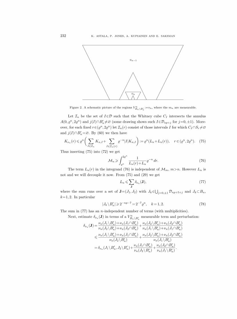
where we recall that V is given by (41). Then ν(I)/ν(J) is VI∪J measurable and, by (29),we see that Kν(I) is Vj(I) measurable (recall that j(I) denotes the union of I with itsneighboring dyadic intervals). From (60) we deduce that Mn is VBn measurable, whereBn :=B(0, 4%n). Indeed, the Whitney cubes CI that intersect the annulus

An :=B(0, 2%n)\B(0, %n)

have I⊂B(0, 2%n) and thus j(I)⊂B(0, 4%n).We now decompose V ( ·)|Bn to scales using the white noise. In general, for 06ε<ε′,

let

V (x, ε, ε′) :=W ((V +x)∩ε<y <ε′). (64)

Set, for n>1,

ψn(x) =V (x, 0, %n−1/2) (65)

and, for k>0,

ζk(x) =V (x, %k+1/2, %k−1/2). (66)

Letting

Λn = z ∈H : y6 %n−1/2, (67)

we see that in any open set U the field ψn is(⋃

y∈U Vy)∩Λn measurable. In a similar

way, ζk(x) is Vx∩(Λk\Λk+1) measurable, and, since these regions are disjoint, the fieldV decomposes into a sum of independent fields

V =ψn+n−1∑k=0

ζk :=ψn+zn. (68)


Let νn be the measure defined as ν but with V replaced by ψn. Inserting the seconddecomposition in (68) to the measure ν we have, for any I, J⊂Bn,

ν(I)ν(J)

6νn(I)νn(J)

supx∈Bneβzn(x)

infx∈Bneβzn(x)

. (69)

The first decomposition in (68) then gives

supx∈Bneβzn(x)

infx∈Bn eβzn(x)

6 e∑n−1

k=0 tn,k := s−1n , (70)

where

tn,k := logsupx∈Bn

eβζk(x)

infx∈Bn eβζk(x)

. (71)

Thus, if we let

Mn =∫ 2%n

%n

dr

Kνn(r), (72)

we arrive at the following lower bound for Mn:

Mn >Mnsn. (73)

This is the desired decoupling upscale. Note that the fields ζk become more regular as kdecreases. This will lead to the following result.

Proposition 4.2. The random variables tn,k satisfy

P(tn,k >u%(n−k)/2−1/4) 6 ce−u2/c, k=0, ..., n−1, (74)

where c is independent of %, n and k. Moreover, tn,k and tn′,k′ are independent if k 6=k′.

The proof of this proposition is postponed to §4.4 below.The decoupling downscale is done to the random variables Mn in (72). Obviously

Mn and Mm are dependent. However, as in (60), most of the terms Kn,I :=Kνn(I) areindependent of Mm if m>n. The few which are not we will process further in a moment.

So let us first look at the dependence of the Kn,I on the white noise. For U⊂R setV nU :=VU∩Λn. Then Kn,I is V nj(I) measurable andMm is V mBm

measurable. Some drawingwill convince the reader that if dist(j(I), 0) is not too smallKn,I andMm are independentfor m>n. Indeed, consider the ball B′n=B(0, 2%n+1/2) so that Bn+1⊂B′n⊂Bn. Theregions V nBn\B′n

are disjoint (see Figure 2). Thus the σ-algebras BV nBn

\V nB′n

are independentof each other for n=1, 2, ... .


vn−1

vn

Figure 2. A schematic picture of the regions V nBn\B′n

:=vn, where the mn are measurable.

Let In be the set of I∈D such that the Whitney cube CI intersects the annulusA(0, %n, 2%n) and j(I)∩B′n 6=∅ (some drawing shows such I∈Dnp+j for j=0,±1). More-over, for each fixed r∈(%n, 2%n) let In(r) consist of those intervals I for which CI∩Sr 6=∅and j(I)∩B′n=∅. By (60) we then have

Kνn(r) 6 %n( ∑I∈In

Kn,I+∑

I∈In(r)

%−n|I|Kn,I

):= %n(Ln+Ln(r)), r∈ (%n, 2%n). (75)

Thus inserting (75) into (72) we get

Mn >∫ 2%n

%n

1Ln(r)+Ln

%−n dr. (76)

The term Ln(r) in the integrand (76) is independent of Mm, m>n. However Ln isnot and we will decouple it now. From (75) and (29) we get

Ln 6∑J

δνn(J), (77)

where the sum runs over a set of J=(J1, J2) with Jk∈⋃j=0,±1Dnp+5+j and Jk⊂Bn,

k=1, 2. In particular

|Jk\B′n|> 2−np−7 =2−7%n, k=1, 2. (78)

The sum in (77) has an n -independent number of terms (with multiplicities).Next, estimate δνn(J) in terms of a V nBn\B′n

measurable term and perturbation:

δνn(J) =νn(J1\B′n)+νn(J1∩B′n)νn(J2\B′n)+νn(J2∩B′n)

+νn(J2\B′n)+νn(J2∩B′n)νn(J1\B′n)+νn(J1∩B′n)

6νn(J1\B′n)+νn(J1∩B′n)

νn(J2\B′n)+νn(J2\B′n)+νn(J2∩B′n)

νn(J1\B′n)

= δνn(J1\B′n, J2\B′n)+νn(J1∩B′n)νn(J2\B′n)

+νn(J2∩B′n)νn(J1\B′n)

.


Then decompose the perturbation further downscale

νn(Jk∩B′n) =∞∑

m=n+1

νn(Jk∩(B′m−1\B′m)), k=1, 2,

and (recalling (28)) define

Ln,n =∑

(J1,J2)∈J (I)

I∈In

δνn(J1\B′n, J2\B′n) (79)

and

Ln,m =∑

(J1,J2)∈J (I)

I∈In

(νn(J1∩(B′m−1\B′m))

νn(J2\B′n)+νn(J2∩(B′m−1\B′m))

νn(J1\B′n)

)(80)

for m>n+1. Then

Ln 6∞∑m=n

Ln,m.

Defining

mn =∫ 2%n

%n

11+Ln(r)+Ln,n

%−n dr (81)

and using the inequality

Ln(r)+Ln 6 (1+Ln(r)+Ln,n)(

1+∞∑

m=n+1

Ln,m

),

we get from (76) thatMn >mnσn, (82)

with

σn :=(

1+∞∑

m=n+1

Ln,m

)−1

(83)

Combining this with (73) we arrive at the desired bound of Mn in terms of randomvariables localized in the white noise:

Mn >mnsnσn :=M ′n. (84)

Proposition 4.3. (i) The random variables mn are V nBn\B′nmeasurable, 06mn61,

and they form an independent set. Moreover,

P(mn 6x) 6Cx for x> 0,

where C is independent of % and n.


(ii) There exist a>0, q>1 and C<∞ (independent of n, m and %) such that forall m>n>1 the random variable Ln,m satisfies the estimate

P(Ln,m>λ) 6Cλ−q%(m−n−1/2)(1+a). (85)

Moreover, Ln,m is V nBn\B′mmeasurable. Especially, Ln,m and Ln′,m′ are independent if

n>m′ or n′>m.

The proof of this proposition is postponed to §4.4.

4.3. Law of large numbers and proof of Theorem 4.1

Here we prove our main probabilistic estimate assuming Propositions 4.2 and 4.3. By(84), we need to consider

PN := P( N∑n=1

M ′n<Nδ

)= Eχ

( N∑n=1

mnsnσn 6 δN

)=: EχDN

, (86)

where

DN :=ω :

N∑n=1

mnsnσn 6 δN

.

For the sake of notational clarity, we used above (and will often use later on) the short-hand χ(A) for the characteristic function χA. In order to obtain the desired bound forPN , we insert suitable auxiliary characteristic functions in the expectation. Define

χn :=∞∏

m=n+1

χ(Ln,m 6 2n−mδ−1/4)n−1∏m=0

χ(tn,m 6 2m−n log 1

2δ−1/4

):=∏m6=n

χn,m. (87)

On the support of χn we have

∞∑m=n+1

Ln,m 6 δ−1/4,

and thus (for δ<1, say)σn > 1

2δ1/4.

Similarly,∑n−1m=0 tn,m6log 1

2δ−1/4, and so

sn > 2δ1/4.

Insert next

1 =N∏n=1

(χn+(1−χn)) :=N∏n=1

(χn+χcn)


in the expectation in (86), and expand to get

PN =∑

A⊂1,...,N

EχDNχAχ

cAc ,

where χA=∏n∈A χn and χcAc =

∏n∈Ac χcn. On the support of χDN

χAχcAc one has

Nδ>N∑n=1

mnsnσn > δ1/2∑n∈A

mn,

so

PN 6∑

|A|>αN

Eχ(∑n∈A

mn 6 δ1/2N

)+∑

|A|6αN

EχcAc , (88)

where we choose α:= 18 min1, a, with a taken from Proposition 4.3 (ii). Observe that α

is independent of %, δ and N .Let us consider the two sums on the right-hand side of (88) in turn. For the first

one we use independence: if mA :=∑n∈Amn then

P (mA<δ1/2N) 6 eδ

1/2tNEe−tmA = eδ1/2tN

∏n∈A

Ee−tmn . (89)

By Proposition 4.3 (i),Ee−tmn 6Cx+e−tx 6 2e−tx(t), (90)

where the auxiliary variable x=x(t) is chosen so that Cx(t)=e−tx(t). Here x(t)!0 andtx(t)!∞ as t!∞. Thus, assuming δ small enough and taking t=t(δ) such that

x(t) =2δ1/2

α,

in the case |A|>αN the right-hand side of (89) is bounded by 2Ne−δ1/2t(δ)N , where

δ1/2t(δ)!∞ as δ!0+. Hence∑|A|>αN

Eχ(∑n∈A

mn 6 δ1/2N

)6 2Ne−g(δ)N , (91)

where g(δ)!∞ as δ!0+.For the second sum in (88) we need to bound

EχcB := E∏n∈B

(1−χn)

for |B|>(1−α)N . For that purpose, we shall make use of the elementary identity

1−∞∏j=1

(1−aj) =∞∑j=1

aj

j−1∏r=1

(1−ar), (92)


valid for any sequence ajj>1 with aj∈[0, 1] for all j>1. Recall equation (87) and setχcn,m :=1−χn,m. We also set χcn,m :=0 for m<0. For any fixed n arrange the variablesχcn,m with m∈Z into a sequence in some order, and apply the identity (92) to write

1−χn =1−∏m∈Zm6=n

(1−χcn,m) =∑l∈Zl 6=0

χcn,n+lχn,l, (93)

with certain variables χn,l satisfying 06χn,l61. Set

χ+n :=

∑l>0

χcn,n+lχn,l and χ−n :=∑l<0

χcn,n+lχn,l. (94)

Then χ±n61 (since χ+n+χ−n=1−χn) and

χ±n 6∑±l>0

χcn,n+l. (95)

We may then estimate∏n∈B

(1−χn) =∏n∈B

(χ+n+χ−n) =

∑sn=±n∈B

∏n∈B

χsnn

6∑

s:N+>(1−2α)N

∏n:sn=+

χ+n+

∑s:N+6(1−2α)N

∏n:sn=−

χ−n ,(96)

where N+ is the number of n in the set B such that sn=+. We estimate the expectationsof the two products on the right-hand side in turn.

For the first product, let D⊂1, ..., N with p:=|D|>(1−2α)N . List the elementsof D as n1<n2<...<np. Then, as 06χ+

nj61,

Eχ+n1... χ+

np6∑l1>0

Eχcn1,n1+l1χ+n2... χ+

np6∑l1>0

Eχcn1,n1+l1χ+ni2

... χ+np, (97)

where ni2 is the smallest nj larger than n1+l1. Iterating we get

Eχ+n1... χ+

np6

p∑r=1

∑(l1,...,lr)

Er∏j=1

χcnij,nij

+lj , (98)

where nij+1 is the smallest nj larger than nij +lj , and ni1 =n1. Since the intervals[nj , nj+lj ] cover the set D, the r -tuples (l1, ..., lr) in the above sum satisfy

r∑j=1

lj > p−r. (99)


Next, by Proposition 4.3 (ii), the factors in the product in (98) are independent, andthus

Er∏j=1

χcnij,nij

+lj =r∏j=1

Eχcnij,nij

+lj .

From (85) and (87) we deduce that

Eχcnj ,nj+lj 6C(%)δq/4(2q%1+a)lj ,

whereby

Eχ+n1... χ+

np6

p∑r=1

∑(l1,...,lr)

(C(%)δq/4)r(2q%1+a)∑r

j=1 lj . (100)

Using (99), we see that the right-hand side is bounded by

%(1+a/2)p

p∑r=1

(C(%)δq/4)r∑

(l1,...,lr)

(2q%a/2)∑r

j=1 lj .

For an upper bound, drop the constraints on lj to bound (100) by

%(1+a/2)p

p∑r=1

(C(%)δq/4)r( ∞∑l=1

(2q%a/2)l)r.

Choosing first % small enough and then δ6δ(%), this is bounded by

C(%)δ1/4%(1+a/2)p 6C(%)δ1/4%(1+a/2)(1−2α)N 6C(%)δ1/4%(1+2b)N

with a constant b>0 by our choice of α. The expectation of the first sum in equation(96) is then bounded by

C(%)2Nδ1/4%(1+2b)N . (101)

Consider finally the second sum in equation (96). We proceed as for the first sum,this time considering a setD⊂1, ..., N with elements n1>n2>...>np with p>αN . Nowwe write χ−n1

6∑l1>0 χ

cn1,n1−l1 and end up with the analogue of equation (98):

Eχ−n1... χ−np

6p∑r=1

∑(l1,...,lr)

r∏j=1

Eχcnij,nij

−lj , (102)

where nij+1 is the largest nj smaller than nij−lj and ni1 =n1, and this time Proposi-tion 4.2 was used for independence. From the same proposition we also get

Eχcn,n−l 6 ce−c2−2l%−l+1/2(log δ)2 .


For small enough % we have 2−2l%−l+1/2>(l+%−1/8)%−1/8 for all l>1. Hence

r∏j=1

Eχcnij,nij

−lj 6 cr exp(−c(log δ)2%−1/8

(r%−1/8+

r∑j=1

lj

)).

As %<1, by (99) we also have

r%−1/8+r∑j=1

lj >12

(p+

r∑j=1

lj

).

Thusr∏j=1

Eχcnij,nij

−lj 6

(exp

c%−1/8(log δ)2p2

)cr exp

(−c(log δ)2%−1/8

r∑j=1

lj

).

Now recall that p>αN , take δ small enough, and proceed as above by summing firstover the lj ’s, and then performing a geometric sum over r in order to conclude that thesecond sum in (96) has the upper bound

2 exp(−c%

−1/8(log δ)2Nα2

).

For small δ this is by far dominated by the bound (101), and therefore

EχcB 6 2N+1δ1/4%(1+2b)N . (103)

Going back to equation (88), and recalling (91) with (101) and (103), we conclude that,for δ6δ(%),

PN 6 22N+2δ1/4%(1+2b)N , (104)

which gives the claim of Theorem 4.1.

4.4. Proofs of the propositions

We will now prove Propositions 4.2 and 4.3 of §4.2, describing the statistics of mn, Ln,mand tn,k. We start by noting that the random measures νn( ·) and %n−1ν1(%1−n ·) areequal in law. Especially, the mn are independent and identically distributed, so that itsuffices to study m1. Similarly ζk|Bn equals in law with ζ1|Bn−k+1 and thus tn,k equalstn−k+1,1 in law. The value k=0 is slightly different, but it can be treated exactly in thesame manner as the case k>1. Finally, Ln,m and L1,m−n+1 are equal in law.

We first need the following lemma. Actually, only the statement (105) is needed forthe proofs of Propositions 4.2 and 4.3. The stronger claim (106) will be necessary onlylater in the proof of Theorem 5.3.


Lemma 4.4. There exist q, q1>1 and C>0 (each independent of %) such that forall intervals J, I⊂

[− 1

4 ,14

]satisfying |J |62|I|, and with mutual distance at most 100|I|,

one has

P(ν(J)ν(I)

>λ

)6Cλ−q

(|J ||I|

)q1. (105)

Even a stronger statement is true: given βmax∈(0,√

2 ), one may choose q=q(βmax),q1=q1(βmax)>1 and C=C(βmax)>0 so that

P(

supβ∈(0,βmax)

ν(J)ν(I)

>λ

)6Cλ−q

(|J ||I|

)q1. (106)

Proof. We use the comparison (53) with the measure η in order to estimate

ν(J)ν(I)

6G2η(J)η(I)

, (107)

where we recall that all the moments of the variable G2 are finite. Next, in case |I|6 1100 ,

we may scale further by using the exact scaling law (55), and apply the translation invari-ance of η to deduce that η(J)/η(I)∼η(J ′)/η(I ′), where now I ′, J ′⊂[0, 1] with 1

100 6|I ′|and |J ′|6|J |/|I|6100|J ′|. In case |I|> 1

100 , no scaling is needed.In this situation, if r<∞ it follows from Theorem 3.7, or (130) in Appendix B, that

η(I ′)−1∈Lr uniformly with respect to I ′. We can thus fix exponents 1<q<q<p<2/β2

and get, by (107), Holder’s inequality and Theorem 3.7,

∥∥∥∥ν(J)ν(I)

∥∥∥∥q

6C

∥∥∥∥η(J)η(I)

∥∥∥∥q

=C

∥∥∥∥η(J ′)η(I ′)

∥∥∥∥q

6C‖η(J ′)‖p 6C

(|J ||I|

)ζ(p)/p, (108)

where ζ(p)>1. The constant C depends only on the exponents q, q and p. Thus

P(η(J)η(I)

>λ

)6Cλ−q

(|J ||I|

)qζ(p)/p. (109)

The desired bound (105) follows by choosing the exponent q>1 close enough to p in orderto ensure that q1 :=qζ(p)/p>1.

In order to consider the maximal estimate (106), choose p>1 and ε0>0 small enoughso that [0, βmax]+B(0, 3ε0)⊂Dp. A standard application of the Cauchy integral formulaand Theorem 3.7 (iii) and (iv) yield that

E∣∣∣ supβ∈(0,βmax)

ν(I)∣∣∣p 6 c|I|q2 and E

∣∣∣ supβ∈(0,βmax)

d

dβν(I)

∣∣∣p 6 c|I|q2 , (110)


where q2=q2(p, βmax)>1 and c=c(p, βmax). In turn, when considering the needed esti-mate for the negative moments,

E(

supβ∈(0,βmax)

ν(I)−r)<∞ for all r > 1, (111)

we are not interested in the explicit dependence on |I|. We compute by applying Theo-rem 3.7 (ii), Holder’s inequality and (110),

E(

supβ∈(0,βmax)

ν(I)−r)

6 Eν(I)−r+rE∫ βmax

0

∣∣∣∣ ddβ ν(I)∣∣∣∣ν(I)−r−1 dβ

.C+(

E∣∣∣∣ supβ∈(0,βmax)

d

dβν(I)

∣∣∣∣p)1/p(∫ βmax

0

Eν(I)−(r+1)p′ dβ

)1/p′.

Note above that, by the argument of Appendix B, for each t, the expectation

Eν(I)−t = Eνβ(I)−t

is locally bounded for β∈[0,√

2 ).The proof of the lemma is now finished, exactly as in case of (105), by applying

the estimates (110) and (111), and noting that in the scaling argument the maximalanalogue of the variable G2 is just the original variable G2 corresponding to the valueβ=βmax.

Let us then discuss m1. Observe that the denominator of the integrand in (81) canbe dominated as

1+L1,1+L1(r) 6 1+L1,1+∞∑m=0

2−mkm(r), (112)

where for r∈(%, 2%) and m>0 one sets

km(r) :=∑

I∈Dp+m

K1,I1CI∩Sr 6=∅. (113)

For any fixed r∈(%, 2%) the sum (113) has at most four non-zero terms.For m>0 denote by Hm the set of all pairs J=(J1, J2) that contribute to km(r)

in (113) for some r∈(%, 2%). To estimate δν1(J), we may scale by the factor %−1/2 inorder to consider instead the identically distributed quantity ν(J ′1)/ν(J

′2), where now

J ′1, J′2⊂[− 1

4 ,14

]. Thus Lemma 4.4 applies. As we additionally have |J1|=|J2|, there is

q>1 and a constant C>0 such that

P(δν1(J)>R) 6CR−q for all J∈∞⋃m=0

Hm. (114)


Choose next α>0 and γ∈(0, 1) such that

4α∞∑m=0

2m(γ−1) 6 1

together with γq>1. Fix R>0. We observe that by these choices

δν1(J) 6α2γmR for all J∈Hm, m> 0 =⇒ L1(r) 6R for all r∈ (%, 2%).

Since we have the obvious estimate #Hm6c2m for the number of pairs in Hm, by com-bining the above implication with the uniform estimate (114), one may estimate

P(L1(r(σ))>R for some r∈ (%, 2%))6∞∑m=0

∑J∈Hm

P(δν1(J)>α2γmR)

6CR−q∞∑m=0

c2m2−qγm 6CR−q.

In a similar vain we may apply Lemma 4.4 to immediately obtain the correspondingtail estimate for L1,1. Indeed, by (79) this depends only on a finite (% -independent)number of ratios δν1(I1, I2), with I1, I2⊂[−4%, 4%] and |I1|, |I2|>2−7%; see (78). Puttingthings together, we obtain (for R>1, say) the bound

P(m1<

1R

)6CR−q 6CR−1, (115)

where C is independent of %.Consider next Ln,m with m>n and use Ln,m∼L1,m−n+1. By (80), L1,m−n+1 is

bounded from above by a sum of terms (with %-independent upper bound for theirnumber)

ν1(J)ν1(I)

,

where 2−8%6|I|62−4% and |J |6%m−n+1/2, and in addition I, J⊂[−4%, 4%]. The constantC above is independent of m, n and %. Via scaling the desired bound (85) is now a directconsequence of Lemma 4.4, as we observe that |J |/|I|6C%m−n−1/2.

Finally we turn to tn,1 given in (71). By scaling, we may take the sup and theinf over x∈Bn∩R of eβψ, where ψ :=ψ( · , %3/2, %1/2), and we may replace there ψ byψ :=ψ( ·)−ψ(0). The covariance of ψ is clearly c%−3/2-Lipschitz and the length of theinterval Bn∩R is 8%n. Lemma 3.3 yields that

P(|ψ|>λc%n/2−3/4) 6C(1+λ)e−λ2/2,

which finishes the proof of the remaining Proposition 4.2.


4.5. Integrability of Kν

In the next section we shall also make use of the the following observation.

Lemma 4.5. Let β<√

2. Then almost surely Kν∈L1([0, 1]×[0, 2]).

Proof. Recall that S=R×[0, 2] is tiled by the Whitney squares CI . By definition,on such a square Kν is a finite sum of ratios ν(J1)/ν(J2) with |J1|=|J2|62−4 and of con-trolled mutual distance as in Lemma 4.4. Thus, for |Jk| small enough Jk lie on a commoninterval of length 1

2 and we have a uniform bound for Eν(J1)/ν(J2)6‖ν(J1)/ν(J2)‖q,q<2/β2, from Lemma 4.4 (or more directly from (108)). For the finitely many Jk notfitting to such an interval we use again (108). Hence there is also a uniform bound forEKν(I) and one obtains

E∫

[0,1]×[0,2]

Kν dz6∑

I⊂D([0,1])

|CI |EKν(I) 6C∑I

|CI |<∞.

5. Conclusion of the proof

In this final section we give a precise formulation to our main result as a theorem andprove it using the work done in the previous sections. In order to make the setup clear,let us recall that our random circle homeomorphism was defined in §3 via formulae (56)and (57). Its extension to the unit disc is constructed by the method described in §2.4,and formula (24) in particular.

The welding method described in §2 requires estimates for the Lehto integral of thedistortion function in D. Theorem 2.6 reduces these bounds to the boundary function,and here the crucial estimates are provided by our Theorem 4.1 in §4.

Theorem 5.1. Assume that β2<2. Let φ: T!T be the random circle homeomor-phism from Definition 3.8, and let Ψ: D!D be its extension as in (20)–(24). Let

µ=µΨ :=∂zΨ∂zΨ

be the complex dilatation of the extension on D, and set µ=0 outside D.Then almost surely there exists a (random) homeomorphic W 1,1

loc -solution f : C!Cto the Beltrami equation

∂zf =µ∂zf, a.e. in C, (116)

that satisfies the normalization f(z)=z+o(1) as z!∞. Moreover, there exists α>0such that the restriction f : T!C is a.s. α-Holder continuous.


Proof. We sketch the proof along the lines of [5, Theorem 20.9.4], to which presen-tation we refer for further details and background.

For any integer n>1 choose Nn=[%−(1+b/2)n]∈N, where b is as in Theorem 4.1. Set

ζn,k := e2πik/Nn for k=1, ..., Nn.

Write also Gn :=ζn,1, ..., ζn,Nn. Thus the distance on T to the set Gn is bounded by

π/Nn∼%(1+b/2)n.For a given n>1 and k∈1, ..., Nn let us denote by An,k the event

An,k =ω :LKν

(k

Nn, %n, 2%

)<nδ

,

and set An=⋃Nn

k=1An,k. Note that here we consider Lehto integrals in the half-plane.Theorem 4.1 combined with stationarity yields that

∞∑n=1

P(An) 6∞∑n=1

Nn∑k=1

P(An,k) 6∞∑n=1

Nn%(1+b)n 6

∞∑n=1

%bn/2<∞.

Borel–Cantelli’s lemma yields that almost every ω belongs to the complement of theevent ⋃

n>n0(ω)

An.

Also, we obtain by Lemma 3.6 that

Kτ 6E2Kν ,

where almost surely E<∞.From Theorem 2.6 and (58) we see that K(z, F ), the distortion of the extension of

h, is bounded by a constant times Kτ (z). Hence Lemma 4.5 implies that almost surely∫[0,1]×[0,2]

K(z, F ) dz6C0

∫[0,1]×[0,2]

Kτ dz6C0E2

∫[0,1]×[0,2]

Kν dz <∞.

We may thus forget the probabilistic setup by fixing an event ω0∈Ω so that we are inthe following situaton: we are given the complex dilatation µ on D, so that the distortion

K =1+|µ|1−|µ|

satisfies pointwise

K(e2πiz) 6C0Kτ (z) 6C0E(ω0)2Kν(z), z ∈H.


Further, from the definition in (24) we have K≡1 for |z|6e−4π. Also, Kν∈L1∩L∞loc onthe square [0, 1]×(0, 2], and for each n>n0 and k∈1, ..., Nn it holds that

LKτ

(k

Nn, %n, 2%

)>E(ω0)−2LKν

(k

Nn, %n, 2%

)>nδE(ω0)−2 =:nδ′.

We next proceed as in the standard proof of Lehto’s theorem by approximating µby e.g. the sequence

µl :=l

l+1µ, l∈N.

Let fl denote the corresponding normalized solution of the Beltrami equation with co-efficient µl, i.e. with the asymptotics fl(z)=z+o(1) as z!∞. Then every fl is a quasi-conformal homeomorphism of C.

To show that (116) has a homeomorphic W 1,1-solution, we need to control theapproximations fl. For this we first apply [5, Lemma 20.2.3], which tells that the inversemaps gl=f−1

l have the following modulus of continuity:

|gl(z)−gl(w)|6 16π2

log(e+1/|z−w|)

(|z|2+|w|2+

∫D

1+|µl(ζ)|1−|µl(ζ)|

dζ

), z, w∈C.

Here the integrals are uniformly bounded as

1+|µl(ζ)|1−|µl(ζ)|

6K(ζ) 6C0Kτ (z), ζ = e2πiz,

and Kτ∈L1([0, 1]×[0, 2]). Thus the inverse maps gl=f−1l form an equicontinuous family.

In order to check the equicontinuity of the family fll>1 itself, we first consider apoint z∈D. Writing 2a=1−|z|, observe that K is bounded in B(z, a) and, as

Kl :=K( · , fl) 6K,

we have, for any l>1 and u∈(0, 1

2a),

LKl(z, u, 1) >LK(z, u, a) >

1‖K‖L∞(B(z,a))

loga

u!∞, as u! 0+.

Moreover, by Koebe’s theorem or [5, Corollary 2.10.2], we obtain

f(2D)⊂ 5D. (117)

Thus, diam(fl(B(z, 1)))65, which may be combined with Lemma 2.3 to obtain

diam(fl(B(z, u)))! 0, as u! 0+, uniformly in l.


This proves the equicontinity at interior points z∈D. Equicontinuity at exterior pointsfollows e.g. from Koebe’s theorem.

In order to next consider the uniform behavior on T, note that it suffices to provelocal equicontinuity on points of [0, 1] for the family

Fl(z) = fl(e2πiz), l∈N.

We first estimate the diameter of the image Fl(B(k/Nn, %n)), assuming that n>n0.Applying the fact that diam(Fl(B(k/Nn, 2%)))6diam(fl(B(ζn,k, 1)))65 and using thistogether with Lemma 2.3, we obtain

diam(Fl(B(k/Nn, %n)))6diam(Fl(B(k/Nn, 2%)))16e−2π2nδ′ 6 80e−nc′. (118)

From these estimates we get the required equicontinuity. Namely, working now onthe circle T, since the set Gn is evenly spread on T, the balls B(ζn,k, %n+1) cover a %n+2-neighborhood of T in such a way that any two points that are in this neighborhood, withdistance not exceeding %n+2, lie in the same ball. Since this holds for every n>n0, weinfer from (118) that there are ε0>0 and α>0 such that, uniformly in l,

|fl(z)−fl(w)|6C|z−w|α if |z|=1, 1−ε0 6 |w|6 1+ε0 and |z−w|6 ε0. (119)

One may actually take α=c′/log(1/%). This clearly yields equicontinuity at the pointsof T, and hence on C. We may now pass to a limit and one obtains W 1,1-homeomorphicsolution f(z)=liml!∞ fl(z) to the Beltrami equation as in [5, p. 585].

At the same time the estimate (119) shows that f : T!C is Holder continuous. Sincef is analytic outside the disc, with f(z)=z+o(1) at infinity, in fact it follows that f isHolder continuous on C\D.

Collecting the results established, we now arrive at the main theorem of this paper.

Theorem 5.2. Let φ=φω be the random circle homeomorphism, with the exponen-tiated GFF as derivative, as defined in (56) and (57).

Then, for β2<2 and almost surely in ω, the mapping φ admits a conformal welding.That is, there are a random Jordan curve

Γ =Γω,β (120)

and conformal mappings f± onto the complementary domains of Γ such that φ=f−1+ f−

on T.Moreover, almost surely in ω, the Jordan curve Γ in (120) is unique, up to composing

with a Mobius transformation Φ=Φω of the Riemann sphere.


Proof. We argue as in §2. Extend φ to a homeomorphism Ψ: D!D and using thisdefine the complex dilatation µ(z) as in Theorem 5.1. Applying the theorem, we thenfind a homeomorphic solution f to the auxiliary equation (116). This is conformal out-side the disc, so we set f−=f |C\D. Inside the disc, K(z, f) is locally bounded, so theuniqueness of the Beltrami equation gives f(z)=f+Ψ(z), z∈D, where f+ is a conformalhomeomorphism defined on D. Since the boundary ∂f+(D)=∂f−(C\D)=f(T)=Γ is aJordan curve, f± extend to T, where we have

φ= f−1+ f−.

Finally, according to the proof of Theorem 5.1, f− is Holder continuous in C\D, and thusthe uniqueness of the welding curve follows from the Jones–Smirnov Theorem 2.4.

Once the random families of curves Γω,β have been constructed, it is natural toenquire for their dependence on the parameter β. In fact, according to Theorem 3.7 (iii),the circle homeomorphisms φ depend analytically on β. More precisely, in any compactsubinterval of [0,

√2 ), the dependence β 7!τ(I), and hence β 7!φ(x), is analytic when

the measures are computed using the same fixed realization of the white noise W in theupper half-plane.

We show that, in the same manner, the welding curves themselves depend continu-ously on β. This should be compared with the analogous question for SLE curves whichis still open.

Theorem 5.3. Almost surely the random welding curve is continuous in the param-eter β∈(0,

√2 ).

Proof. After the maximal estimate (106), the proof follows closely the proof of The-orem 5.2, and hence we only sketch the argument. By (106) in Lemma 4.4, we mayrun through the proofs of Propositions 4.2 and 4.3, and obtain the analoguous maximalversions. Actually, for Proposition 4.2, this is simple since the dependence of tn,k on β

is linear. In turn, for Proposition 4.3, one uses fully the bound (106).The argument of §4.3 now yields an estimate for the Lehto integral which is uniform

in β∈(0, βmax): for positive %<%0(βmax) and δ<δ(%, βmax), with βmax<√

2,

P(LKν (w0, %N , 2%)<Nδ for all β ∈ (0, βmax))6 %(1+b)N . (121)

In addition, we obtain a maximal version of Lemma 4.5:

supβ∈(0,βmax)

Kν ∈L1([0, 1]×[0, 2]). (122)


Let us fix a realization of the white noise so that the estimates (121) and (122)hold true for all βmax<

√2, with the understanding that the appropriate constants may

depend on βmax. Assume that βj!β∞∈(0,√

2 ). Let us denote by f±,j (resp. µj andKj) the corresponding conformal maps (resp. random dilatation and distortion in D)obtained in Theorem 5.2.

First of all, Theorem 2.6 yields a local uniform boundedness of K∞ and supj>1Kj

in D. These facts together with (121) and (122) yield equicontinuity for the maps f±,jand their inverses (and even uniform local Holder continuity for f−,j).

Next, since the random homeomorphism φ depends continuously on β, the complexdilatations µj converge pointwise to µ∞. At this stage a well-known argument (see e.g.the proof of [5, Theorem 20.9.4]) shows that fj has a subsequence that converges toa solution of the Beltrami equation with dilatation µ∞. In particular, one applies theestimate (122) to obtain uniform integrability for the derivatives of the solutions.

Finally, the uniqueness of the welding in the present situation is inherited for the nor-malized solutions of the Beltrami equation, and this yields the local uniform convergencefor the whole sequences f±,j to f±,∞, as was to be shown.

Remark 5.4. One may easily verify that the distortion function K of our Beurling–Ahlfors extension has a.s. the property K /∈Ls(D), where the exponent s=s(β)!2 asβ"√

2. Especially, this shows that our random setting lies far from the setup where thegeneral (deterministic) theory of existence and uniqueness for solutions to degenerateBeltrami equations still works. In fact, even the optimal deterministic results roughlyrequire an exponential type integrability of the distortion K(z)=(1+|µ|)/(1−|µ|), fordetails see [5, Theorems 20.3.1 and 20.5.2].

Finally, we state and prove the generalization of the previous two theorems for acomposition of two independent copies of our random homeomorphism discussed in theintroduction. Since the argument is essentially identical, we only sketch the neededchanges in the proof.

Theorem 5.5. Let 06β+, β−<√

2. Assume that φ+ and φ− are two independentcopies of the random homeomorphism (56) with parameters β±. Then, almost surely inω, the welding problem for the homeomorphism φ+φ

−1− has a solution Γ=Γβ+,β− , where

Γβ+,β− is a Jordan curve bounding the domains Ω+=f(D) and Ω−=f−(D∞), with Holdercontinuous Riemann mappings f±. For a given ω, the solution is unique up to a Mobiusmap of the plane and the curves Γβ+,β− are continous in β+ and β−.

Proof. Let us extend the circle homeomorphism φ+ inside the unit disc by theBeurling–Ahlfors extension as in §2.4, and we now denote by φ+ also the extension.Moreover, let µ+ stand for the dilatation of φ+ in D. In a similar manner, define the


Beurling–Ahlfors extension of φ− into C\D by φ−(1/z)=1/φ−(z), and denote by µ− itsdilatation. Set

µ(z) =µ+(z), if z ∈D,µ−(z), if z ∈C\D.

Due to our specific choice of the extension, µ has a compact support, see (22) and (24).Since the estimates for the Lehto integral of the distortion function

K(z) =1+|µ|1−|µ|

in the new situation are identical to those presented in Theorem 4.1, the proof of The-orem 5.1 carries through with only notational changes, yielding as before a solution tothe Beltrami equation

∂F

∂z(z) =µ(z)

∂F

∂z(z) for almost every z ∈C,

with the normalization F (z)−z=o(1) as z!∞. In addition, F |T is Holder continuous.Next we define the analytic maps f+: D!C and f−:C\D!C via

F (z) = f+φ+(z), z ∈D, and F (z) = f−φ−(z), z ∈C\D.

Especially, one obtains the key formula

f+φ+ = f−φ− on T, (123)

which shows that the maps f± solve the stated welding problem. Uniqueness of thesolution is deduced as before by observing that f+|T is a Holder map since f+=F φ−1

+ ,where φ−1

+ is Holder continuous according to Corollary 3.9. Finally, the proof of The-orem 5.3 can be repeated in order to verify the stated continuity with respect to β±.In the argument one needs to additionally observe that almost surely φ−1

+ is uniformlyHolder continuous with respect to β+, when the parameter is varying over any compactsubinterval of [0,

√2 ). In turn, this follows from the proof of the lower bound in Theo-

rem 3.7 (i) combined with a quantitative version of the inequality (111), obtained easilyfrom the scaling law (54).

Appendix A. Analytic dependence

The analyticity of the dependence of multifractal random measures on the parameter βwas established by Barral in [7]. We will prove the analyticity of β 7!η(I) (the proofs forβ 7!τ(I) and β 7!ν(I) are analogous) and the statements formulated in Theorem 3.7 (iii)


via the techniques of that paper. To start with, we may clearly assume that I is dyadic,more specifically I=[0, 2−m] with m>1. We apply the notation of §3, and denote, forintegers n>1, by Fn the σ-algebra generated by the restriction of the white noise w to(x, y):y>2−n.

Define

U(x, n) :=w((U+x)∩y > 2−n),

and set, for β∈C and x∈R,

fn(x, β) := eβU(x,n)−β2γU (n)/2, (124)

where γU (n)=Cov(U(x, n))=1+n log 2. Then fn(x, β) is Fn-measurable, and, by def-inition, fn(x, β)n>1 is a complex martingale sequence with respect to the filtrationFnn>1. By considering the real part in the exponent, we compute, for β=β1+iβ2,

E|fn(β, x)|p = c(β, p)2n((p2−p)β21+pβ2

2)/2 with p> 1, (125)

where c(β, p)=e((p2−p)β2

1+pβ22)/2. The proof below basically uses only this fact together

with the underlying hidden cascade-like structure of the hyperbolic white noise.Set

Xn :=∫I

fn(x, β) dx=∫ 2−m

0

fn(x, β) dx. (126)

Obviously Xnn>1 is a complex martingale sequence. Let

gn+1(x, β) =−1+fn+1(x, β)fn(x, β)

. (127)

Then the gn(x, β), n∈N, are independent. In particular, gn+1(x, β) is independent of Fn.Let also In,j :=[(j−1)2−n, j2−n] for 16j62n.

Assume next that n>m and write

Xn+1−Xn =∫ 2−m

0

fn(x, β)gn+1(x, β) dx

=

(2n−m∑j=1

j odd

+2n−m∑j=1j even

)∫In,j

fn(x, β)gn+1(x, β) dx=:Y +Y ′.

Conditioned on Fn, the quantities gn+1( · , β)|In,j , for odd j, are independent by con-struction. Hence the Burkholder–Gundy inequality and the simple estimate ‖ · ‖`2 6‖ · ‖`p


imply that

E(|Y |p|Fn) . E

((2n−m∑j=1

j odd

∣∣∣∣∫In,j

fn(x, β)gn+1(x, β) dx∣∣∣∣2)p/2∣∣∣∣∣Fn

)

6 E( 2n−m∑

j=1

∣∣∣∣∫In,j

fn(x, β)gn+1(x, β) dx∣∣∣∣pFn).

Taking expectations and applying Holder’s inequality inside the integral yields

E|Y |p .2n−m∑j=1

|In,j |p−1

∫In,j

E|fn(x, β)gn+1(x, β)|p dx

.2n−m∑j=1

|In,j |p(E|fn(0, β)|p+E|fn+1(0, β)|p)

. 2n−m2−np2n((p2−p)β21+pβ2

2)/2.

A similar estimate holds for Y ′ and, by recalling that |I|=2−m, it follows that

‖Xn+1−Xn‖p 6 |I|ζp(β)/p2−(n−m)(ζp(β)−1)/p for n>m. (128)

In turn, by applying directly (125) together with Holder’s inequality in (126), we obtain

‖Xm‖p 6 |I|ζp(β)/p. (129)

As the geometric convergence of the estimate (128) is uniform in any compact subset ofDp, we get by a standard application of Cauchy’s integral formula and Borel–Cantelli’slemma, the a.s. limit

X := limn!∞

Xn,

and the convergence is locally uniform with respect to the parameter β∈Dp. Hence, Xis a.s. analytic in Dp and, by summing up the estimates (128) and (129), we obtain inany compact subset β∈S⊂Dp the estimate

‖X‖p 6C(S)|I|ζp(β)/p,

as was to be shown.


Appendix B. Negative moments

Here we prove the finiteness of all negative moments for the measure η, defined in theproof of Theorem 3.7. One first needs to verify non-degeneracy of η over any subinterval([20], [21]; see also [6, Theorems 1 and 2]), and to this end we recall the functions fn andgn from (124) and (127). We may write η as the a.s. limit

η(dx) =w*-limn!∞

fn(x, β;ω) dx=w*-limn!∞

n∏j=0

(1+gj) dx,

where the densities gj=gj(x, β, ω) are independent. Moreover, Efn(x)=1 for each x andn, and fn(x) are a.s. bounded from below by a positive constant.

Let I be a dyadic subinterval and set Yn(ω):=∫Ifn(x, ω) dx. By Kolmogorov’s 0-1

law, the probability for limn!∞ Yn=0 is either zero or one. The second alternative canbe ruled out by observing that EYn=|I| for all n and that Ynn>1 is an Lp-martingalewith p>1, according to Theorem 3.7.

We are now ready to start the proof of

Eη(I)−q 6C <∞, 0<q<∞, (130)

for β2<2. Here the constant C=C(q, |I|, β) depends only on the exponent q, the length|I| and the parameter β. Fix t>0. Define, for ε>0, the set Uε,t :=(x, y)∈U :ε<y6t.As in (52) one deduces the existence of the limit measure

ηt(dx) := limε!0+

eβUε,t(x)−β2 Cov(Uε,t)/2 dx. (131)

Set M :=η1/2([0, 1]), M1 :=η1/8([

0, 14

])and M2 :=η1/8

([34 , 1])

. By scaling and translationinvariance the random variables M1, M2 and M are identically distributed. Moreover,by comparing the exponents as in the proof of Lemma 3.5, we see that

M >B(M1+M2), (132)

whereB := einfx∈[0,1] βU1/8,1/2(x)−β2 Cov(U1/8,1/2)/2

has all moments finite. By construction, the random variables M1, M2 and B are inde-pendent.

Similarly, by comparing η and η1/2, we see that it is enough to prove that

EM−q <∞ for q > 0. (133)


We first prove this for small values of q. To this end, consider for s>0 the Laplacetransform

ΨM (s) := Ee−sM 6 Ee−sB(M1+M2) 6 EΨM1(sB)ΨM2(sB) = EΨM (sB)2. (134)

Since especially EB−1<∞, we may estimate P(B<1/s)6c/s. By substituting s2 in placeof s in (134) and applying this inequality, we obtain

ΨM (s2) 6c

s+Ψ2

M (s), (135)

where one may assume that c>2.Set f(s):=(c/s1/2+ΨM (s)). Then (135) yields

f(s2) =c

s+ΨM (s2) 6 f2(s). (136)

Since ΨM (s)!0 as s!∞ (while P(M=0)=0), we may choose s0>0 with ΨM (s0)6 12 ,

whence (136) iterates to f(s2k

0 )62−2k

for k>1. Together with the monotonicity of f ,this yields δ>0 such that f(s)6cs−δ for s>0, especially ΨM (s)6cs−δ.

We obtain thatEM−δ/2 = c

∫ ∞

0

Ee−sMsδ/2−1 ds<∞.

In order to cover all values of q in (133) we employ a simple bootstrapping argument.Assume that EM−q<∞ for some q>0. By applying the inequality between the arithmeticand geometric mean, the independence of B, M1 and M2, and the fact that B has allnegative moments finite, we may estimate

EM−2q 6 E(B(M1+M2))−2q 6 cE(M1M2)−q = c(EM−q)2<∞. (137)

By induction, this finishes the proof.

References

[1] Adler, R. J. & Taylor, J. E., Random Fields and Geometry. Springer Monographs inMathematics. Springer, New York, 2007.

[2] Airault, H., Malliavin, P. & Thalmaier, A., Canonical Brownian motion on the spaceof univalent functions and resolution of Beltrami equations by a continuity method alongstochastic flows. J. Math. Pures Appl., 83 (2004), 955–1018.

[3] — Brownian measures on Jordan–Virasoro curves associated to the Weil–Petersson metric.J. Funct. Anal., 259 (2010), 3037–3079.

[4] Anderson, G.D., Vamanamurthy, M.K. & Vuorinen, M.K., Conformal Invari-ants, Inequalities, and Quasiconformal Maps. Canadian Mathematical Society Seriesof Monographs and Advanced Texts. Wiley, New York, 1997.


[5] Astala, K., Iwaniec, T. & Martin, G., Elliptic Partial Differential Equations andQuasiconformal Mappings in the Plane. Princeton Mathematical Series, 48. PrincetonUniversity Press, Princeton, NJ, 2009.

[6] Bacry, E. & Muzy, J. F., Log-infinitely divisible multifractal processes. Comm. Math.Phys., 236 (2003), 449–475.

[7] Barral, J., Techniques for the study of infinite products of independent random functions(Random multiplicative multifractal measures III), in Fractal Geometry and Applica-tions: a Jubilee of Benoıt Mandelbrot, Proc. Sympos. Pure Math., 72, Part 2, pp. 53–90.Amer. Math. Soc., Providence, RI, 2004.

[8] Barral, J. & Mandelbrot, B.B., Introduction to infinite products of independentrandom functions (Random multiplicative multifractal measures I), in Fractal Geome-try and Applications: a Jubilee of Benoıt Mandelbrot, Proc. Sympos. Pure Math., 72,Part 2, pp. 3–16. Amer. Math. Soc., Providence, RI, 2004.

[9] — Non-degeneracy, moments, dimension, and multifractal analysis for random multiplica-tive measures (Random multiplicative multifractal measures II), in Fractal Geometryand Applications: a Jubilee of Benoıt Mandelbrot, Proc. Sympos. Pure Math., 72,Part 2, pp. 17–52. Amer. Math. Soc., Providence, RI, 2004.

[10] Beurling, A. & Ahlfors, L., The boundary correspondence under quasiconformal map-pings. Acta Math., 96 (1956), 125–142.

[11] Binder, I. & Smirnov, S., Personal communication, 2010.[12] Bouchaud, J. P. & Fyodorov, Y.V., Freezing and extreme-value statistics in a random

energy model with logarithmically correlated potential. J. Phys. A, 41 (2008), 372001,12 pp.

[13] Cardy, J., Scaling and Renormalization in Statistical Physics. Cambridge Lecture Notesin Physics, 5. Cambridge University Press, Cambridge, 1996.

[14] Carpentier, D. & Le Doussal, P., Glass transition of a particle in a random potential,front selection in nonlinear renormalization group, and entropic phenomena in Liouvilleand sinh-Gordon models. Phys. Rev. E, 63 (2001), 026110, 33 pp.

[15] Duplantier, B. & Sheffield, S., Liouville quantum gravity and KPZ. Invent. Math.,185 (2011), 333–393.

[16] Fyodorov, Y.V., Le Doussal, P. & Rosso, A., Statistical mechanics of logarithmicREM: duality, freezing and extreme value statistics of 1/f noises generated by Gaussianfree fields. J. Stat. Mech. Theory Exp., 2009 (2009), P10005, 32 pp.

[17] Jerison, D. S. & Kenig, C. E., Hardy spaces, A∞, and singular integrals on chord-arcdomains. Math. Scand., 50 (1982), 221–247.

[18] Jones, P.W. & Smirnov, S.K., Removability theorems for Sobolev functions and quasi-conformal maps. Ark. Mat., 38 (2000), 263–279.

[19] Kahane, J.-P., Some Random Series of Functions. Cambridge Studies in Advanced Math-ematics, 5. Cambridge University Press, Cambridge, 1985.

[20] — Sur le chaos multiplicatif. Ann. Sci. Math. Quebec, 9 (1985), 105–150.[21] — Positive martingales and random measures. Chinese Ann. Math. Ser. B, 8 (1987), 1–12.[22] Kahane, J.-P. & Peyriere, J., Sur certaines martingales de Benoit Mandelbrot. Adv.

Math., 22 (1976), 131–145.[23] Lehto, O., Homeomorphisms with a given dilatation, in Proceedings of the Fifteenth

Scandinavian Congress (Oslo, 1968), Lecture Notes in Mathematics, 118, pp. 58–73.Springer, Berlin–Heidelberg, 1970.

[24] Mandelbrot, B., Intermittent turbulence in self-similar cascades: divergence of highmoments and dimension of the carrier. J. Fluid Mech., 62 (1974), 331–358.


[25] Molchan, G.M., Scaling exponents and multifractal dimensions for independent randomcascades. Comm. Math. Phys., 179 (1996), 681–702.

[26] Oikawa, K., Welding of polygons and the type of Riemann surfaces. Kodai Math. Sem.Rep., 13 (1961), 37–52.

[27] Reed, T. J., On the boundary correspondence of quasiconformal mappings of domainsbounded by quasicircles. Pacific J. Math., 28 (1969), 653–661.

[28] Samorodnitsky, G., Probability tails of Gaussian extrema. Stochastic Process. Appl., 38(1991), 55–84.

[29] Schramm, O., Scaling limits of loop-erased random walks and uniform spanning trees.Israel J. Math., 118 (2000), 221–288.

[30] — Conformally invariant scaling limits: an overview and a collection of problems, in Inter-national Congress of Mathematicians (Madrid, 2006). Vol. I, pp. 513–543. Eur. Math.Soc., Zurich, 2007.

[31] Sheffield, S., Conformal weldings of random surfaces: SLE and the quantum gravityzipper. Preprint, 2010. arXiv:1012.4797 [math.PR].

[32] Smirnov, S., Conformal invariance in random cluster models. I. Holomorphic fermions inthe Ising model. Ann. of Math., 172 (2010), 1435–1467.

[33] Talagrand, M., Sharper bounds for Gaussian and empirical processes. Ann. Probab., 22(1994), 28–76.

[34] Vainio, J. V., Conditions for the possibility of conformal sewing. Ann. Acad. Sci. Fenn.Ser. A I Math. Dissertationes, 53 (1985), 43 pp.

[35] Vuorinen, M., Conformal Geometry and Quasiregular Mappings. Lecture Notes in Math-ematics, 1319. Springer, Berlin–Heidelberg, 1988.

Kari AstalaUniversity of HelsinkiDepartment of Mathematics and StatisticsP.O. Box 68FI-00014 University of [email protected]

Peter JonesYale UniversityDepartment of Mathematics10 Hillhouse AveNew Haven, CT [email protected]

Antti KupiainenUniversity of HelsinkiDepartment of Mathematics and StatisticsP.O. Box 68FI-00014 University of [email protected]

Eero SaksmanUniversity of HelsinkiDepartment of Mathematics and StatisticsP.O. Box 68FI-00014 University of [email protected]

Received September 8, 2009Received in revised form August 3, 2010

Documents

Random conformal weldings - MathSciDoc: An Archive for …archive.ymsc.tsinghua.edu.cn/pacm_download/117/6745... · · 2018-01-14The SLE curves come in two varieties: the radial