r

,

~.— .——..

d.:0

.

NATIONALADVISORYCOMMITTEEFOR AERONAUTICS

TECHNICAL NOTE 2554

THEORETICAL AERODYNAMIC CHARACTERISTICS OF A FAMILY

OF SLENDER WING-TAIL-BODY COMBINATIONS

By Harvard Lomax and Paul F. Byrd

Ames AeronauticalMoffett Field,

LaboratoryCalif.

Washington

November 1951

..-. —.. . .. .;..—

&

—.. — -—- --TECHLIBRARY-, NM

InlnlllllfllllfllllllllllllDL5b1331

Page

1

1

2

2

3

6

6

“8

I-1

l-l

15

16

17

19

19

22

23

27 ‘

27

30

31

3k

35

TABLE

,

. . . ●

✎

✎

.* . ...** ● ☛✎✎ ●

✎

✎

.

●

●

●

● ☛

✎ ✎

.

.

. .

. .

.0

.

.

●

●

●

✎

.

.

.

●

✎

✎

.

.

●

.

.

.

.

.

.

.

.

.

.

.

●

✎

✎

●

✎

✎

✎

✎

●

✎

✎

✎

INTRODUCTION . .* *.**. .**.

I - SWEPT-BACK WING ON A BODY OF REVOLUTION . .

Partial Differegtial Equation, Boundary Conditions, and Formof the Solution . . . . . . . . . . . . . . . . .

.

.

●

.

●

●

✎

.

.

●

✎

.

.

.

.

●

✎

✎

✎

Discussion of notation and transformations .I

Boundary conditions . . . .

General solution . . . . .

Particular solution for the

● ✎ ...0 . .

.* ...* .0

.

.

nearly constant-chordWing

The Trailing Edge . . . . . . .

Speci&l.trailing-edge shape

Other trailing-edge”shapes

.

.

●

✎

✎

✎

✎

✎

✎

✎

●

✎

✎

✎

●

✎

✎

✎

.

.

●

✎

✎

✎

✎

✎

.

.

.

●

✎

✎

✎

✎

.

●

✎

✎

✎

✎

✎

✎

✎

.

.

●

✎

✎

✎

✎

✎

✼

✎

✎

✎

✎

✎

✎

✎

●

✎

✎

✎

✎

✎

✎

✎

✎

✎

✎

✎

✎

●

✎

.

●

✎

✎

✎

✎

✎

✎

✎

✎

✎

✎

✎

✎

✎

.

.

.

.

.

●

✎

✎

●

✎

✎

✎

✎

✎

✎

.

.

.

.

.

.

●

●

✎

✎

✎

✎

●

✎

✎

.

.

.

.

.

.

.

.

.

.

.

.

.

●

✎

.

.

.

.

.

.

.

.

.

.

●

✎

✎

✎

✎

.

.

.

.

.

.

.

.

.

.

.

.

.

●

✎

.

.

.-

The Wing Area . . . . . . .

Downwash Behind Wing . . . .

Chordwise Load Distribution

.

.

.

.

.

.

.

.

.

.

.

.

the wing..

the body . .

Loading on

Loading on

Discussion

.

.

loading

. .

● .

. .

. .

. .

of the chordwise .

Aerodynamic Characteristics .

.

.

.

.

.

.

.

.

.

.

.

●

✎

✎

✎

✎

.

.

.

.

.

.

. .

. .

. .

● O

. .

. .

s-pm loading

Section lift

Section drag

Total lift .

Total drag .

.

.

.

.

.

.

●

✎

✎

✎

.

.

.

●

●

. .

. .

. .

. . .1’

.*.

.,. ——-—- ——-—— ——--- --. —-—.-. -—— —— ----- .——- .--. .——.. — ——. -—-— ...— .—. ——

. .

. .

. .

38

’40

41

42

43

45

46

47

4a

48

49

49

52

53

53

54

9

54

.

.

●

Chord loading . . . .

Center of pressure .

.

●

.

.

.

.

.

.

.

.

.

●

✎

.

.

.

.

.

.

.

.

●

✎

●

✎

●

●

●

✎

✎

✎

✎

●

●

✎

●

✎

.

.

●

✎

✎

✎

✎

●

✎

✎

✎

✎

✎

✎

✎

●

✎

✎

●

✎

✎

✎

✎

✎

✎

✎

✎

✎

✎

●

✎

✎

✎

✎

✎

✎

●

●

●

✎

✎

●

✎

●

✎

●

✎

✎

✎

✎

✎

●

✎

✎

●

✎

✎

●

✎

✎

✎

●

✎

✎

●

✎

✎

●

✎

✎

●

●

●

✎

✎

✎

✎

✎

✎

✎

✎

✎

✎

✎

✎

✎

●

✎

●

✎

.

.

●

●

✎

✎

✎

●

✎

✌✎

✎

✎

✎

✎

✎

●

✎

✎

●

✎

●

✎

✎

✎

✎

✎

✎

✎

●

●

●

✎

●

●

✎

●

.

.

.

●

✎

✎

✎

●

✎

●

●

●

●

✎

✎

✎

✎

✎

II - ADDITION OF A HORIZONTAL TAIL

Met@d of Solution and Boundary Conditions

Solution for Trailing Vortex Sheet . . . .

Span loading . . ...=.

Chordwise load distribution

● ..0.

,.

Total lift on

Drag . . . .

Chord loading

the

. .

. .

.

.

.

.

.

.

.

.

.

.

.

.

.

.

.

.

.

.

.

●

✎

●

●

✎

✎

●

✎

✎

✎

✎

✎

✎

✎

✎

✎

✎

.

.

.

.

●

✎

✎

●

✎

✎

✎

✎

✎

✎

✎

✎

✎

.

●

✎

✎

✎

✎

●

●

●

✎

●

.

.

.

.

.

.

.

.

.

.

.

.

.

.

.

●

✎

●

✎

✎

✎

✎

.

.

. .

. .“

.*,.

Center of pressure

Solution for Rolled Uy Vortices

Span loading . . . ... . .

Chordwiae load distribution

Total lift . . . .

Totaldrag . . . .

Chord loading . . .

Center of jressure

.

.

.

.

.

.

.

.

.

.

. .

. .

● ✎

✎ ✎

✎ ✎

✎ ✎

✎ ✎

✎ ✎

✎ ✎

✎ ✎

.

.

.

.

.

●

●

✎

✎

✎

●

✎

●

●

✎

. .

.

.

.

.

●

✎

✎

✎

✎

‘.

.

●

.

.

●

●

✎

.

.

.

.

●

✎

●

●

✎

✎

✎

✎

.

.

.

●

●

●

.

.

●

✎

●

✎

.

.“

55

57

62

65

66

69

CONCLUDING REMARKS . . . . .

Al?PENDIXA . . . . . . . . .

APPENDIXB . . . . . . . . .

Rmmumms . . . . . . . . .

mlnxs ● . . . . . . . . ● .

FIGURES. . . . . . . . . . .

. .

● O

. .

. .

. .

. .

.

.

.

.

●

✎

✎

.

.

.

.

.

.

.

..

—. —-..—— .——— . . _—— —. .- -- — - --—

NATIONAL ADVISORY COMMITTEE FOR

TECHNICAL NOTE 2554

AERONAUTICS

THEORETICAL AERODYNAMIC CHARACTERISTICS OF A

OF SLENDER WING-TAIL-BODY COMBINATIONS

By Harvard Lomax and Paul.F. Byrd

SUMMARY

FAMILY

The aerodynamic characteristics of an airplane configurationcomposed of a swept-back wing and a triangular tail mounted on acylindrical body are presented. For simplicity, the leading edge ofthe wing is considered to be straight sad the trailing edge to beshaped so that the span-loading curve is flat between the fuselage andthe wing-tip regions; the result is a nearly constant-chord swept-backwing. A method by which other trailing-edge shapes can be studied isindicated. The analysis is based on the assumption that the free-stresmMach number is nesr unity or that the configuration is slender. Thecalculations for the tail are made on the assumption that the vortexsystem trailing back from the wing is either a sheet lying entirely inthe plane of the flat tail surface or has completely “rolled up” intotwo point vortices that lie either in, above,or below the plane of thetail surface.

INTRODUCTION

The studyof lifting surfaces flying at either subsonic or super-sonic speeds at small angles of attack has been reduced, by the wel2-lmown p~ocess of lineari~ation, to the study of the

where 9 is a perturbation velocity potential in auniform free-stream velocity V. directed parallel

equition

(1)

field hatig ato the x axis,

and where ~ is the Mach numb& of the free stream.

One basic simplification of equation (1) is brought about byneglecting velocity gradients along the span of the wing. If the wing

. ——.—.——. . -.—_______ ~—. ____ . _ ...- —_____ —— _____ .. .. . ________ .

,—–_

is lylng in the z = O, plane, this amounts to neglecting the term Qnin equation (1), and results in the well-known partial differenti,dequation by means of which two-dimensional or section characteristicsare studied.

Another basic simplification of equation (1) csm be atta~ed byneglecting the term (1-M02) pa. Such a procedure is possible when theMach number is close to 1 or the wing plan form is so slender thatvelocity gradients in the free-stream direction are negligible in com-parison with the gradients in the y and z directions. Equation (1)has already been snalyzed in these two connections in references 1 and 2for certain plan fomns. The purpose of this report is to extend thistheory, which has been nsmed slender wing theory, to include an entireairplme configuration.

Results are presented for a nearly constant-chord, swept-back wingmounted on a cylindrical body having a triangular horizontal tail locatedtit of the wing trailing edge. Both wing and tail are flat surfaces,and the results are only those due to changes in the airplane angle ofattack.

A list of important symbols

I-SWEPT-BACK WING

.

is given in appendix A.

ONA BODY OF REVOLUTION

Psz%ial Differential Equation, BoundaryConditions, and Form of the Solution

Under the assumption that the free-stream Mach numberthe perturbation velocity gradient in the x direction is

is 1 or thatsmaU, the

partial differential equation which must be satisfied for the so~utionof lifting surface problems can be written

~yy+qzz=o. . (2)

Equation (2) is simply Laplace~s equation in two dimensions, thevariables representing lateral and vertical coordinates in a planetransverse to the direction of motion.

The boundary conditions,associated with equation (2) sre givenalong a line in this transverse plane and specify that the fluid veloc-ity is everywhere tangential to the surface of the body. The problem is,of course, to find at other points in the plane the potential thatsatisfies equation (2) and fits these boundary conditions. of paticularinterest is the streamwise component of velocity slong the surface ofthe wing and body since this is directly related to the loading thereon..

. .—. . —.— -— –—— -—..—— ___ ____ — —

I

NACA TN 25% . 3

.

i-

,.

Solutions to equation (2) are readily available. Two differentsmalytic forms of these solutions will be used in the following analysis.One form is concerned with the use of the complex variable, the otherwith the use of Greenfs theorem and the inversion of a real, singular,integral equation. In general the procedure till be to use conceptsassociated with the complex variable to map the boundary conditions ontoa slit along the real axis, then to solve the resulting problem byinverting an integral equation, and fin@ly, to use the co~lex variableagain to extend such a solution out into space by the principle of ana-lytic continuation.

Discussion of notation and transformations.-The first part of thisreport will be devoted to the analysis of the configuration shown insketch (a). The.following is a description ofthis co~iguration. Eve&here behind-theleading-edge-fuselagejuncture the fuselageis a circulsr cylinder having a radius ro.Ahead of this juncture the fuselage comes toa point, the manner being arbitrary. Thewing is a fiat @ate without twist or canibermounted at zero incidence on the fuselageand the whole configuration is placed at a “small angle of attack a with respect tothe free-stream direction. The origin ofthe coordinate system is located at thewing apex. The leading edge is a straightline with slope, dy/dx, eqyal to m. Itwill be convenient at some places in thereport, however, to use the expression

Y= s(x) for the equation of the leadingedge, hence, s(x) and mx are used inter-changeably. The trailing edge is repre-sented by the line y = t(x) and is, infzeneral,-notstraWhi.l me ~ semispan of the wing is denoted<y so.- The syniboi to, as cambe seen in the sketch, refers to thelateral distance from the x axis to the point at which the trailingedge intersects a line that is yarallel to the y axis and passesthrowh the last outbosrd point of the leading edge. Finally, co isthe &ordwise dis~ce fro; thp origin to the-juncture.

trailing-edge-fuselage

lIt ma considered ad~s’able at t~s the to consider only the rather

particular configuration outlined. As the analysis progresses itwill be pointed out where the solution can be generalized to include,fer eqle, wings with twist and caniber.

●

✎ ✍✎ ✍� ✎ �� � ✎ ✎ ✎ ✎ ✎ ✎ ✎ ✎ ✎ ✎

4 NACA TN

A second coordinate system will also be used in the succeedingdevelopment. Let the y,z plane be represented by the complexvariable ~,

then introduce

so that the gtransformation

~=y+iz=

the El plane,

~l=fi+iz~

plane maps onto the El

peie

= pleiel

2554

plane by means of the Joukowski

(3)

BY means of such a transformation, the circle of radius rn whichrepresents a section of the fusel&ge in the ~ plane maps-onto a portionof the real axis in the, ~1 plane (see sketch (b));

and the part of the real axis which

(plane j=lies outside the circle2 in the E

t-

plane maps into the remaining partof the real axis in the ~1 Plane.

I J+1-1 1-

r. cos e = yl/2y-rl<yl<rl

vs.-l Y1- A/x==Y= J

2

.

%’he Joukowski transformation is double valued in that the regionsinside and outside the circle p = r. both map onto the entfie ~1plane. In this report only the field outside the circle is of interest. .,

— ..- —— .—— . —

.

NACA TN 25.54

and

5

I

(5)

2r.

y~=y+—Y’

YI = 2ro Cos e, y12~r12J

Further,

2r.

2S1 =s+ -7’ “

=t+r~,r~ = ao (6)

From the basic theory underl@ng the use of complex variables in fluid-flow theory, induced velocities in the two planes are relatedby theexpression

v-iw = (V1-iwl)

from which, since in polar coordinates

dE1

si-

3=[‘- @’)2cos2“1+ i (32‘in2’

it follows that

TT=w, [1 - ~:y COB q -..(;JVr =

[

.1 cos e+wl sti e

~ 1[1-(31sin 2e

I

(7)

(8)

) (9)

Lastly, Laplacets equation must also be satisfied in the El plane,hence

(lo)

. . . . -—. —..-————- .--- —-. ..-. -—— —— —- —.——--------- ... —- ..—.-. -.

r

.

6 NACA TN 2554

..Boundsry conditions.- In this part of the report (part I), the

effect of a cylindricalbody mounted on a nearly constant-chord swept-back wing willbe studied. (Reference 3 contains an analysis of theeffect of a cylindricalbody mounted on a triangular wing, and reference 4presents results for a swept-back wing with no body; both referencesuse the assumptions of slender-wing theory.) The boundary conditionswillbe pres=ted in the y,z spa;e first and can be written

(i) v~ = o, P = ro, 0~e~2fi1

(ii) w = o, z = o,

(iii) v = o, w = Voa, p ==,

Equations (n) represent the conditions for a

t2 <y2<s2

o~e<2fi/

cylinder located

(II)

atP = r. and two wing panels located between H and *S on the realtis, both cylinder andwings%eing at rest in a free’stream which ismoving with velocity w = Vo~ at infinity.

It follows from equations (9) that these boundary conditionsbecome, in the El plane,

(i) w~ = o, 0<y12 < r12

(ii) WI = o, t12 < y=2 <812

‘1

(12) ‘

(iii) Vl= o, W= svo~, Pz=m, o<e~2fi ‘

Equations (12) represent the boundary conditions for three ’wingpanelsalong the real tis, alllat rest with respect to the free strem movingwith velocity w= = Voa at infinity in the transformed plane.

It is more convenient to work with boundsry conditions which vanishat infinity,~owever, so the final form of the conditions which must besatisfied is derived from equqtions (12) by subtracting the free-streamvelocity Voa. There results

(i) w= = - Voa, 0< y=2< r12

(ii) WI = - Voa, t12< y=2< S12

(iii) Vl SWl = o, Pl ==, o<e<2fiI

(13)

.

i

“

General solution.- The general solution to equation (10) whichgives the vertical induced velocity wl at a point in the 31 planedue to the jump in the value of the induced velocity VI across the ylsxis can be written (see, e.g., reference 5)

.

—— —.-__—-—_—

I

2

.

NACA TN 2354

‘~ (Y1-Y.&wI(YZ)W1(Y1)Z1) = - &

J’dY2

(YI-Y2)2+2=2-s1

7

(14)

where y2 is the variable of inte~ation. Set zl equal to zero andthere results th6 value of the vertical induced velocity on the y=axis. Thus

J’‘14Y2) ~2W1(Y1) = wl(Y@) = - ;fi’ —

Y1-Y.2-s1

(15)

Equation (15) is the form of the solution which will.be used to@ze the problem previously outlined. It is apparent by reference tothe boundary conditions listed as equations (13) that in equation (15)the value of W1 is the lmown quantity and Avl is the unlmown. Hence,.equation (15) is an integral equation which must be inverted in order ●

that the solution can be written. Such an inversion is not difficult ifthe value’of WI i’sknown everywhere in the interval -Sl<y=<Sl. b ~the present case, however, there is a subinterval rX2<yl=<~2 inwhich WI is not specified, and further, in which Avl is not neces-sarily zero (due to the presence of a trailing vortex sheet). It willbe shown in the subsequent development that the assumption that Avlis zero in this interval (i.e., no vortices sre shed by the wing aheadof the interval)‘yieldsa nearly constant-chord, siept-back wing; withsuch a restriction the inversion can again be perfomned.

Given the inversion of equation (15), it is possible to write both.WI and V1 for certain portions of the real tis. All along this sxisthe functions WZ and VI are, of course, real. Hence, if

f(~l) = vJY@J-iq(Y@J (162)

then by analytic continuation

f(g~) = V(EI,O)AT’’(E1?O) (16b)

Therefore, the inversion of equation (15), together with equation (16),gives sufficient information to determine the induced velocities through-out space.

1-

.,

. ... —..- . . . .. . —..—— - —- —————— -—————— .——-----L -.——— ___ ._ ....—.. .. ...—.

.———-— — . .

8 NACA TN 2554

Particular solution for the nearly constant-chordwing.- Adopt thenotation Av=b equals Avl in the region of the Y1 axis representi~the body or fuselage in the El pl~e; A~la equals the value of AV1in the region of the yl @s represent- the space between the fuse-lage and the wing; and Avlw equals the value of Avl in the region ofthe ‘yl axis representing the wing plan form. Then if Avla = O (thecalculation of the trailing-edge shape corresponding to such a choicewi13 be presented later), equation (15) becomes

(17)

Since the airplane is laterally symmetrical, the span loatig is sym-metrical and Aql(yl) =Aql(-yl). Therefore, API has the propertyAV1(Y1) = -AvI(-Y1). By means of this relation for Avl and the addi-tional change in notation

equation (17) can be writtens

‘1W=(ll=)= - &-

f0Eqyation (19) wi~ now

wl=- V@ for 0<~l<r12

J-h= Y12

72 ‘ Y221

(18)

(19)

be inverted under the condition thatand for tl2<q1<s12, and under the addi-

tional condition that (AvIW) - (A~la)q2=t12 = O, which amounts to~2=t12 -

assuming the Kutta condition along the wing trai”lingedge (seey e.g.,reference 4). This inversion is accomplished by a double applicationof the following solution (see appendix B): If

b A~1(n2)d?2f(ql) = - &

f vl-n2a

then, under the condition that Avl(a) = O

(20a)

(20b)

.

.

.—z —— .- .- —— . ~..

NACA TN 25%

Now write equation (19)in the form

9

and then, since Avl~(0) = O by reasons of symmetry, applyeqyation (20b). For o<~l<r 12, there results the expression

Substitute equation (2) back into equation (19),integration and, for t12< ql< s12, there results

(21)

reverse the order of

“0”=-&J$%r’2g- (22)

tla

where

?

ain~ l’lJ

1q2-r12

g(72) = AVIW(1’12) ~2

apply equation (20b), this time to eqyationcan be shown to satisfy the relation

(23)

(22). In this way

(24)

and equating this expression to equation (23) gives

‘v.w’-moaG,> ‘12<’1<s12

(25a)

.. . . . . . ..—. ..— .. ---- ---- -.—.— --, ..- ——————---- . ..— —.-- —- .-. .----- —-——— .. .. .. --- -.— —

10 NACA TN 2554

A repetition of the above process Yieldss

The results given by equationsin space by anslytic continuation.procedure. Hence, since (Vl)zla =

VJY1>ZI

!.(25b)

(25) can be extended to,other pointsEquations (16) indicate the necessaryAvl/2,

‘ [i+ j= ] (26)-iwJYl,zJ = Vc)a

‘When the method is applied to a value of wl which has some givenvsriation with q= there results

.

and

b2rl

o

s.2

V2(%2+-12)

tl=’<ql<sla

+

+ {

—.—... ..—.—— —— —.

,

NACA TN 2554 la

Equation (26) has’seversl branch points so it is’not uniquely definedwithout specifying the cut from -~ to S1 along the real axis inthe &l plane (see sketch (c)).In the upper half of the 31 plane J,fz,191varies between O and fi andin the lower half, between O r“

(and -x. Notice that when 51 isat a very lsrge distance from theorigin in any direction the mag-nitude of the term on the right-hand side of equation (26) tends ~to zero, so that the boundary “

——.-.—------------- —____ -

[

--------—---- --.--z-s,

conditions at infinity -e satis- SIGut In ~ planefied. It is evident that the

other boundsry conditions in (c)equations (13) are also satisfied. “

The Trailing Edge

Special trailing-edge shape.- Equation (26) is a solution toLaplace’s eqyation and represents the flow around a wing and body.However, the plan form of the wing has not as yet been evaluated,although it has been fixed as that which makes the value of Avl vanishin the region between the ~ and the body. Since Avl is the~adient of Aql in the yl direction, and further, since (AQ1)TOE

.(the value of API at the wing trailing edge) equals the totsl circu-lation rl about a given chordwise section, this amounts to the samething as assuming that there are no trailing vorticies between the wingand the body. It is a further consequence of such an assumption thatthe span loading ahead of this region is a constant for r.2<yo2<to2e

The configuration which will produce such a flow must nowbe determined.In particular, if the leading edge is taken to be a straight line, theequation for the trailing edge is unique ad needs to be expressed.

One of the simplest ways of finding the shape of the trailtig edgeiS to find ~CEO from equation (26) and solve for t as a function

.

1.

.- 1.- . . . - —. ---- .- ._ ——. .- —- . -- — --- -— _ _ . ___ _ . . . __ _— . ._ _. . . . _ .

__

12 NACA TN 2554

fixed value of r. and ~.Ec. !!?heCOIM3tantrepl?eSent-is the value of the jump in potential at the point P inHere Aq is lmown

, –.[see, e.g., reference 3) since there isno gap to make its solution indeter-minate.

Consider an-arbitrary section, asM in sketch (d), downstream of thepoint P. The value of Avlw at sucha section is givenby equation (2%)and the solution for L@lw fo120ws bydefinition and is

(27)

Equation (27) is an elliptic integralwhich can be easily reduced by means ofthe substitutions

s~z-tl’k12 =

s12-r12Ykl’2=-(28)

and.by using the Jacobian elliptic functions”defined,in this case, by

(s12-t12)sn2u = s=2-y=2, cn~ = l-sn’u, dn~ = l-k12sn~

to the form

snd where the incomplete elliptic integrals E and F arethe list of symbols (appendix A). Equation (2g) reduces togiven in references 3 and 4 when there is no gap or no body

(29)

(30)

defined inthe resultsrespectively.

.

—— .— —-— — —.—. — .—- ..= — —-

NACA TN 2554 13

At the trailing edge yl = tl, and eqmtion (a) becomes

(31)

‘where the elliptic integrsls are now complete. Transform this to thephysical plane, using equation (6), and set

then there results

(32)

(33a)

At the juncture of the fuselage and the wing trailing edge (the point Pin sketch (d)), s equals mco and t equals ro, so that

equation (33a) reduces to

(4)T.E. = ~mCO[’- (S 1 (33b)

As was pointed out, the solution for the equation of the trailing edgecanbe obtainedby equating these two values of (A9)TCE.. Hence

‘co[’-(as1= - (Eo-~’2dor

t 2-mcot

Set

[’-(SV’1--ro2=0Eo-~’~

~ [’-kh’=mcoEo-~’2&

(34)”

---- --- .- —...... .— - -.. -—— - .. - —_ ..-—.-—— - — ..—.—— -- . -- . .-—

14

and since s equals mx

. /’ t2-r.2 \ ~

From equation (34) the solution that gives theshape can be written

t_G+m

2

and from the definition of ~T

correct

NACA TN2554

trailing-edge

(35)

‘ t2-ro2 + J( t2-ro2)2+4~’2t2r02mx=

2ko’t

(36)

If &’ and ro/mco are fixed, t/mco is determined from equation (35);

/and a fixed ~?, r. mco and t/mco determines x/c. fromequation (36). Hence, it is relatively easy tothe shape of the trailing edge.

Sketch (e) shows the shape and position ofthe wing leading edge is swept back 45° and theis 31.6 percent of the extended root chord, co.

calculate numerically

the trailing edge whenradius of the fuselage(A dimensionless

/. o

/.5

x

To

2.0

coordinate system is chosen,

Y@* ,0however, so that the results

.5 can be used for various values.I of m. and co.) shown also,

for comparative purposes, isthe position of the trailingedge when there is no fuselage -the condition in both casesbeing, of course, that novortices trail back in the

Troiltng edgesregion directly behind the wing.Table 1 presents coordinates of

~ /m cothe trailing edge”for severalvalues of ro/mco.

o.3/6 -

I

.— - -.—— .— —-— ——.. . . . .. .. .. . ..... —

NACA TN 2554

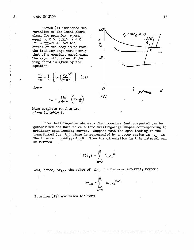
Sketch (f) indicates thevariation of the local chordalong the span for ro/mco -equal to 0.6, 0.Q6, and O.It is apparent that theeffect of the body isto makethe trailing edge more nearlythat of a constant-chordwfng.The asymptotic value of thewing chord is given by theequation .

where

Mm’cm = ()x-;

x+ m

15

/.0

~

co

.5...

‘ y/mco 2

More complete results aregiven in table 2.

just ~resented canbeshapes corresponding to

Other trailing-edge shapes.-genera.lizedand used to calculate

The proceduretrailing-edge

arbitrary span-loading curves. Suppose that the span loading in thetransformed (or ~=) plane is representedby a power series in yl inthe interval rl=~y12~t12. Then the circulation in this interval canbe written ,

and, hence> Avla> the value of AV1 in the same interyal, becomes.

m

Avl,a= Ynbfiln-l

L-1n=b

Eqgation (19)now takes the form

.. ..— —— . . . .—.——-. . . .. . ——— __.._. _ _ .— —._ .-—. —.. —--— —---- . ..— -

._. —

16

.

The left-hand side of the latter equation varies with VI in a givenmanner depending on the bn’s in the expression for r. Hence, theequation can be considered as identical to equation (19), the left sidebeing regarded as an effective w= in equation (19). The analysissucceeding equation (19) can now be repeated in terms of the equivalentWL. There results an equation for the trailing edge which depends onthe bn’s,

1.

By the process outlined, both the trailing-edge shape and the span-loatig curve have been expressed in terms of m + 1 constants. Byvarying the number and magnitude of these constants, a large class oftrailing-edge shapes canbe obtained.

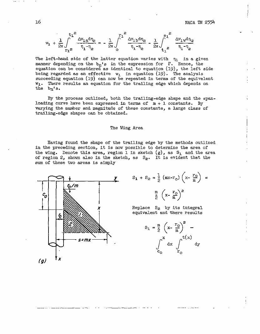
The Wing Area

Hating found the shape of the trailing edge by the methods outlinedin the preceding section, it is now possible to determine the srea ofthe wing. Denote this srea, region 1 in sketch (g), as S1 and the areaof region 2, shown also in the sketch, as S2. It is evident that thesum of these two areas is shply

1“(g) x

m

()

2ro

5 ‘-r

Replace S2 by its integralequivalent and there results

() r. 2s+ x-; -

—.— ———— —- —.—-__— —.

.

.

NACA TN 25% 17

If a dimensionless system hased on the length Co is adopted, one canwrite for the total area (i.e., both panels, see the shaded area insketch (hi)) of the wing the equation

where t/mco is given numerically as a function of x/c. in table 1(y/rnco in the table representing t/mco). Numerical relations betweenthe parameters S/mco2j ro/mco, so/mco, and to/so are presented infigure 1.

The area of a wing with anotherkind of tip shape can be readilyevaluated once the particular tipshape is specified. For example> thearea of the wing shown in sketch (h2)can be calculated by mibtracting arectamgul~ area (given by the sum ofthe two triangular regions labeled 3in sketch (h2)) from the area of asketch (hi).

Downwash Behind Wing

The equation for the downwashbehind the wing and in the z = Oplane ~ollows immediately fromequation (26). In the transformed~1 plane the value of wl is

prl = - Voaj O < y~2< r12;t12< Y12<s12

(/) I

#

and

, w.=-voa[-m]Jr.2<(3@)

. . __ .. —-.. ,------- .—. ——-— .—-. --- -—----—.— --- -----------—.—

18 I?ACATN 259

In order to transfomn this value to the physical plane, cexe must betaken to go backwards through the boundary conditions in the properorder. Equations (38) represent the solution for the boundary conditionspresented in equation (13). To find the solution for the conditionsgiven by eqyation (M) a free stream V& must be added. ~US~ ~mathematical notationj

where the subscripts 12 and 13 refer to the boundsry conditions satis-fied. Finally, to find the d.ownwashin the physical plane, the transfor-mations given as equationsstream subtracted so that

(9) ad (5) must ~e-employ~d and the free

[ 1 y+o’ _ v ~ ~

W(y) = (WJ13 + Voa oY2

where (w=)~~ now becomes ‘

(Wl)~~ = - V~, 0< ~< r=;t2< ?< S*

and

(WJ13=-V. [1,~(’-)jm],,<.-2Combining and simpli~, one finds

w(y) = - V&jO< y2< r2;t2< y2< S*

and

(39a)

w(y) = - .v& Pi%)~=],...<t.(39b)

.

. . . . ..—.— .— —. —— . —. --

NACA ~ 2554 19

The accompanying sketch shows the variation of -w/V@ in theintervals for which it has been given. If no wing is attached to the

1.0 6--i

AA BB cc -

-w~

-: y)

I “ /~.-@i /“’ /// /

---- /“

.5-----–- ---4- ---””~”With body —

-— - —— -- - - Without body -----[

.6 I.g y/me*0 4-

-.5-1

- /.O-1

body (or if the gap is very lsrge) the fluid at the side of the body ismoving upward at a speed equal to ttit at which the body is moving duwn-ward. The presence of the wing restricts this motion and as the wingpanel approaches the body the air in the gap is forced more and more tomove downward with the wing and body. The dotted lines in the sketchshow the variation of -w/V& if no body is present, that is, if r.equals zero.

Chordwise Load Distribution

Loading on the wing.- The loading on the wing can be calculatedby means of the linearized equation for the loading coefficient. Thisequation can be written

()AP 2AU 2 w..=—= ——Tw Vo Vo &f

.(4oa)

—.. . –—.-—-— . .. . ...._ .. -—.. . .. _.. _ . ..... . . ______ ._ --z___.~~ .~_,. ..=

.—-— —... . ——. .—,

1

t

L

,

NACA TN 25P20

It is somewhat easier to calculate the lo-g if the derivative ofAvw

is taken in the 51 plue. If A~lV is considered to be a function

of the two independent variables y=ad SIJ equation

modified slightly to read

()

AP 2 all!?lvas~ ~— =—— ——

~~ Vo as~ ti &

(M)a) can be

(kOb)

WlwThe value of —asl

cam be obtained by differentiat~

thus

eqmtion (29)}

.

aATlw

[[—=2VOCL —J+ 1E(k=,$l)-kl~F(klY~l) +

aal 2-rl2

aE(kl,~l) _ kl,.2aF(klyVl)-[

dk=’

s~z-r12 — —— 2kl’F(kl,*l) —asl asl dslII .

which becomes.

(41) ,

The terms dkl/ds= and a~l/&l both involve dtl/dsl which is

proportions.1-to the slope of the trailing edge in the transformed ~1plane. This latter derivative can be readily obtained from equation (41)itself since the value of (AP/q)w ~d hen~~W~~$sludW~~ be ‘eroon the trailing edge, that is, where Y1

eq@s 1.

This yields the relation

dtl slEl—=— (42)

,as~ tlKl

._ . ..— —— .—. —.—— —---_——

, al?ACATN 2554

by means of which the identities

and (43)

&lkl—=

-(E’-’:K7 Jdsl s12-r12

cm be written. Place equations (41) and (43) into equation (40b), andthere results for the loading

1 Ap

-()

‘14—El.— =

J—- [E(kU$l)- —F(k=,V1) +

m qa ~ s.2-r.2 K1

Transforming this to thedsl/ds =(a2-ro2)/s2

5 plane, one finds, finslly, since

1 ()Ap2s2+ro

4—

“1

E.-—=S* E(~,~o) - ‘F(ko,~o) +

m W w .’0

s2(F-ro2) 1(y2-t2)(y2t2-ro4)

yt(s2-ro2) (s2-#) (.2~-ro4)

where ~ is defined by equation (33) and .

(44)

(45)

In the special cases when there is.no body or when the ~ istriangular, equation (44) agees with the results presented inreferences (4) and (3), respectively. A discussion of the chordwiseload distribution over the ting will be given at the end of this section.

)

. . . . . . . . .--— .——. - -- —.--—-

.——— .. —.———.

22 NACA TN 2554

Loading on the body.- The vsriation of the load distribution overthe body can be calculated in much the same way as that over the wing.It is first necessary, therefore, to find the jump in potential betweenpoints directly opposed above and below the z = O plane. In the ~1pl=e this difference follows immediately from equation (25b) just asequation (27) wm writtenfor Apm. Hence,

Theand

+j’=”’ (46)

‘1first of the integrals in equation (46) has already been evaluatedthe second can be reduced by means of the transformation

(t=2-y22) sn% = r12-y~2

After some manipulation, equation (46) becomes

Awb = 2VOCC[E1-E(kl,~~)+kl’2F(k1,~~)-kl’2K1]=+

where kl is defined by equation (28) and

rr12-y12v-~= —

t12-y12

(47)

(48)

Using the equ&ions (42) and (47), one can write for the loading on thebody (after differentiation and simplificationof equation (47))

-—-—. —-.———— -—-.—— —-

.4 23

.

%2( s2-ro2)t I (49)[(&+r02)2-4y%2] [(#+r02)2-4##]

where &j is defined by equation (33) and

*. ’f?-t

Again equation (49) ~ees withpreviously lmown results in thelimiting cases when the bodyvanishes or when the wingbecomes triangular.

Discussion of the chord.wise loading.- Equations (44fand (~9) form the basic resultsof p&rt”I of this report.Graphs of the loading coeffi-cient for a wing alone and fora wing-body combination (ro/mcoequals 0.~6) are shown insketch (jl). The results forthe case of zero body radiuscould have been obtaineddirectly from reference 4.They are sho& here for thepurpose of a qualitative com-parison. Unfortunately, theload distributions on the twowings cannot be compared quan-tatively on the basis of equiv-alent plan forms since thetrailing-edge shapes differsignificantly. The variation

(x)

10-,\

1 1

t .Tm-dtm#nsbmi

~m

\

SeCNM AA Y> :,,

00 Percent chord 10010

F!iid10

Two - dbnenslonul

-!!iiii

‘tTvo - a%wmsionol‘,.

—‘,

. No bod.

-——

‘Fii+YG’;:::bo” “o~ o~o Percent chord 100 Percent chord 100

[E;=o Percent chord 10000 Percent chord 100

,

——. -...—+— ...— — ..-— —.-—... —. ——— —.— ——-.—-— -— ---- —.-. .--—--

I

24 NACA TN 2554

.

of the loading sd.ongthe center line of the body is shown in sketch (j2).

4

APqocm

2

00 .8 /.2

x/c*

.

/.6 2.0

On the basis of the load distributions presented in references 3and 4, the qualitative variation of loading shown in sketch (jl) isobvious● That is, the loading falls steadily from its infinite peak atthe leading edge to zero at the trailing edge. On sections which arecut by the Mach wave from the trailing-edge fuselage juncture, the slopeof the curve is discontinuous.

The change in the load distribution brought about by the presenceof a wing tip is the same for a wing-body combination as for a wingalone. The behavior of the loading in the vicinity of a tip has astraightfo~d explanation in terms of the trailing vortex sheet.Thus, if the wing is cut off along a line perpendicular to the free-stresm d.irecticn,the vortices which were bound in the wing &El.turn andtrail backwards with the ssme distribution in strength4 as they had when

~is assumes, of course, that the vortices have not begun to roll up toany significant extent.

—.—..— -—.—. ..—-. .. .

NACA TN 2554 25

.

crossing the last spanwise section of the wing(see sketch (k)). Since the vertical inducedvelocity along the last spanwise section was madeconstant (by finding the appropriate solution tothe integral equation), it must also be constant -and, in fact, the same constant - everywhere inthe vortex wake. Hence, if a flat surface havingthe same dngle of attack as the wing is insertedanywhere in the wake it will in no way disturb theflow and consequently there will be no loading onsuch a surface (just as there is no loading on thevortex wake itself). The loading is zero, therefore,on the tip regions marked 2 in sketch (k); the load-ing in the regions marked 1 being given, of course,by equation (44).

It is interesting to see how the distribution cand magnitude of the loading given by this(slender wing) theory compare with linearized ,theory results at some Mach nuniberother than 1.The differences causedby considering Mach numbersother than 1 depend, of course, on whether or notthe new Mach number is subsonic or supersonic.This discussion must be limited to a comparisonwith supersonic Mach numbers only, since theo-retical chordtise ,loaddistributions over swept-back wings flying at high subsonic speeds are notavailable. The change in the loading brought aboutbyincreasing the speed can be divided into two parts:one, a change caused by the rotation of the Machlines which-form the boundaries of the various [h]regions in each of which the shape of the loadingcurve takes widely different forms; and the other,a change in the magnitude of the loading withineach of these regions.

Sketch (Z) indicates these effects. Thus, on the wing flying atsupersonic speeds the sharp drop in loading occurring at a critical Machline moves father back along the chord from point b to point a insections AA and BB sho~m in the sketch. This causes a considerablyhigher value of the loading for the supersonic wing5 in regions 1 and 2.A similar effect occurs on the body traveling at a supersonic speed wherenow, however, the traces of the Mach lines are no longer straight but,

5Solutions showing the effect of crossing critical Mach lines on a ,swept-back supersonic wing are given in references 6 and 7.

. . . . ..— ---— - --—-— — -- ———. ..——— —-— —-..— ..—- —

,_— —— ——

26

The relativethe vsrious sreasand the pertinentreference sectionwing span. Along

AP\ —-supersonic

qa

L

‘---M = I

\ \\

“~.. b,>

AA Noo c

AP1

1-’-1-/

)\

\

‘b,0IIII BB

o c

L.----1,/ I0’ \/ \/ \

/ \./

Icc

o c

.

I?ACATN 2554

.

due to the curvature of the body, formhelices. Region 3 in the supersonic casewould be a region of zero loading and region 4 ‘would be a region of high loading relativeto the sonic value.

magmtude of Ap~qa withinbounded by the wing”edgesMach lines changes as themoves outbosrd along theinboard sections ahead of

region 1 in the sketch (i.e., ahead of thesonic Mach line from-the trailing edge root)the loading on the sonic wing is higher thanthat on the supersonic wing. It is welllmown, Yor example, that in the case of atriangular wing without body, slender-wingtheory gives a loading E times The loadingobtained at a supersonicMach number (whereE is the complete elliptic integral of the

second kind with modulus ~1-~~ andi.s given

closely by. 1 +$s’2 (n+ -:) ‘or

sti values of mj3). On the other hand,along sections farther outbosrd, the magni-tude of Ap/qa on the sonic mng must becomelower than that on the supersonic wing. Thisfollows immediately from simple sweep theory,since the component of velocity normal to theleading edge is closer to the speed of soundthan zhat for the sonic wing. In fact, it iseasy to show that at distances tar enoughoutbosrd so that simple sweep theory appliesethe supersonic wing has a loading

t -m’’’)-’”times that obtsined from

slender wing theory.

By an”applieation of the above consider-ations, it is possible to obtain an estimateof the absolute value of the loading on awing-body combination az supersonicMach

0

8Sketch (jl) indicates the reamer in which the loading approaches thatgiven by simple sweep theory as the reference station moves outboard.

.

. — —— .——— -—— - —..

,,

NACA TN 2954 27

numbers. Another manner in which the results of slender wing theory canbe extended to Mach numbers other than 1 (or to pl~ forms which are notsufficiently slender) is to form the ratio of the resulting values forthe wing plus body to those for the wing ai.oneand apply this ratio tosolutions for the sape wing or body at the required flight Mach numbers(or slenderness factor). As has already been mentioned, the form@ion,of such a ratio for the load distribution is not possible from the solu-tions presented herein since the wing trailing ewes change to a certainextent with the addition of the body. It is reasonable to eqect, how-ever, that a ratio of the integrated loading characteristics (i.e., lift,drag, and pitching moment) formedby dividing the result for awing-bodycombination by those for a wing alone will be useful in estimating theinterference effects even if the wing trailing edges differ slightly.

Aerodynsnic Characteristics

The results developed in the preceding section can now be convertedinto forms which represent the aerodynamic’characteristicsof the wing -and hOdy. Hence, the foil.owbg will present the span loading, averagechord loading, lift, drag, pitching moment, and center of pressure forthe wing-body conibination.

Span loading.- The development of thebody will be considered separat~ly. Firstcan easily be determined from the value ofsection. Thus

span loading on the wing amdthe span loading on the wingAP given in a preceding

.

wingplm foti

and since A9 at the leading edge is zero

where (A9)T.E. is the value of ‘Ap on the trailing edge of the wing.

Sfice (AOToEe also represents the total circulation about the wingchord, there results for the circulation ~ developed by the wing and

‘ the total wing lift ~

.. —.-... - —-. .-— .- .,.. .-— . — —.- - .—.. ---- - . - - -+ - .—-- -- ... .. .. ..——--- —-—

28

rw = (A9T.E.

NACA TN 2554

Lw = pv~f

rw * “ (51)

span

The equation for rw can now bedetermined from equation (29).

~Y BetweenY= r. and y= to (see

sketch (m ) the value of rw iS aconstant (this being the conditionby which the shape of the trailingedge was determined). Between y= toand y = so, P’ is given by the valueof A9 along the section AA sincethere is no loading between thissection and the trailtng edge. Hence

A’

‘w=‘o~m[l-(a7, ‘“’ys’o

and

‘w=2v@(’-)[E@’JJ-~[’F(~,”J1y‘“sysso (52b)

where ~ and ~. are defined in the table of synibols.

Some ”caremust be taken in order’to find the span loading on thebody. Since we sre concerned here with the loading developed behind thewing-leading-edge fuselage juncture, it is necesssryto subtract thevslue of A% at this station, shown as station AA in sketch (n), fromA% at station BB also shown in sketch (n). For the total span loading,then, it will be necesssry to add to this value the load accumulatedon the nose of the body. Denote by (rb)o the increment of circfiation .developed by the nose of the body ~dby (b)l the in~em~t of circu-lation developed behind the wing-lea--edge fuselage juncture, thatis, between stations AA and BB.7 Hence,

7Slender wing theory gives zero loading behind station BB as long’asthe trailing vortex pattern does not vary.

.

.—— ——. ——. —. ——— ——.————- .._.—

NACA TN 2554 29

(rb)l = (AT)T.E. - (AOL.E.

(Lb) , = poVof

(b)l w

(53)

The &lue of (A@ LoEc, see sketch (n),bcan be obtained from equation (47) bysetting tl and SI equal to rl.IBy transformation of”the result into,

I the physical plane, one obtains

(AQ?LOEO= 4Voa ~ro2-~

A

B

.

—

—.

m

The span loading on the body is then\ given by

!

{

s02-roz(‘b)1 =2voa —

[Eo-E(ko#2)+ko

112F(k@2).~’2~ +

s~

where ~ and Y2 are given in the table of synibols.

.

.

(54)

.

. .. —-.. .----- .–.:—— —————... —- ...- ——— — . ..—. _ ._ —-_——.—.-

30 NACA TN 2554

J.

rhcorn

t

.Wing on oninfinite cylinder

2,0-“

/.o--

Y

0 .4 .8 12 1.6c7m

table 2.and 0.316

Typical resultsin sketch (p).

soc7m

Sketch (o) shows thevariation of the span loadingover the wing and body for a

/body radius factor, r. mco:equal to 0.316 and a wing

/semispan factor, so mcoequal to 1.7.

Section lift.- The wing-section lift coefficient canbe calculated readilybydividing the section chordinto the value of the spanloading at the same span sta-tion. Along sections notinfiuencedby the tip cut-offthis is especially simplesince the span loading isconstant. The value of thesection lift curve followskediately, therefore, from

are shown for a body radius factor equal to O

Zo I

Asymptote

6.0

cl

T@/ /

/

~/mcO = .3/65.0 /

4.00 / 2 ylmco J

.

—. -—-— -—.— —.— ..—

5

.

Section drag.- The value of the section drag can be written

Cd = “CZ + (cd)s (55)

where (Cd)s represents the suction force at the section leading edge.The magnitude of (cd)s can be evaluated (see, e.g., reference 8) by theequation

(56)

where dF/dy is the suction force in the free-stream direction per unitlength normal to the free stream, and c is the local chord.

Define a new set of coordinates, as sho~m in sketch (q), such thatyn lies along and Xn lies perpendicular to the leading edge of onewing panel. Then’if

G= lti ~n ‘“(~’yn) GXn~O

( 57)

the suction-force component F (positivein the positive Xn direction) in thefree-stream direction is givenby theequation

imaqG2(x,y)—=- —

W 1%

Nowby differentiating equationby 2 (to convert Au into u),

(58)

(29) with respect to x and dividingthere results

sa(y2-ro2)

yt(s2-ro2)

---- _ _ ..-—.- ...— .— —.-—— —. .- —--— =--- ..- .————

\

32 ,

and similarity v becomes

v=- ‘o”- (:)=

NACA ~2554

Since the normal component un is given by the equation

‘n‘sthere results

Un

‘By

~n

‘ “J%’c=) W’Y’J-%‘(’’”O)l+*m[

m2(s2+ro2)(~-ro2) s(y2+ro2)+

82 2 1Y y/mco >1

-r. Y

means of e@ation (57), G can now be calculated. Hence, since

= l/J3 ,

G=a(~+ro2)

J

, (F-t2)(fi’-ro4j@(l+m2) 1’4 ~My ’-r04)

Fin~’y, therefore, the suction force can be written

d’ a2(y2+ro?a-q

[

(Y2-t~(J%2-ro4)—=. J ( 59)w y%2 . My2-r02)

and, by usingbe written

equations (55) and (~), the section drag coefficient can

o

.

——___ . .—.. _— . _ _ ___ _ — ___

NACA TN 255k 33

.

,.

cd (22 W.%J[’+W7 [:-U] [’-W(%YI ,,mco>l—=— .—aam (c/c*) ~ r. 2 “

)

()-—

Y

(60a)

In the region where the lewMng-edge suction force cannot be affected bythe trailing-edge shape, equation (6o) reduces to the simpler form

cd c1 fi(y/mco)_-a% am (c/co) [’-f;Yl’ro/mco~y/mco~’ ‘6m) -.

!lhevariatdon of the section drag coeffici~t is shown in sketch (r)for two wings: one without a body, and the other with a body radiusfactor equai

-.to 0.316.

6 .

9 ‘\ZP

4 ., 1

\

\‘\

b

-- ____

..

---- ------- .-- —- ---.—-——- -.--—— ——..—.——— .— ... —- ..- ——— .--— —.— —.—. ..—

— ——

34 NACA TN 25*

Total kift.- The lift on the wing, the body, and the combinationcan now be evaluated by means of equations

[ [~1) and 53) stice the

expressions for I’ are given by equations 52) and M). The integra-tion required is somewhat involved algebraically,but the final resultcan again be expressed in terms of elliptic inte~als. Thus, defining

Ao(k>V) by

r

&(k,v) = ~1KE’(kj$) + EF’(kj$) - m’ (k,*)

m 1 (61)

(tabular values for & can be found in reference 9), the total liftcarried by the wing is

r T

L-w p So’-ro’

{

to2+ro2 rE2-~’2i2] -kro ~Eo-ko’2 -~= so to

G] }

L

(62)’

Equation (62) agrees with the results presented in references 3 and 4when to = r. (the case of a triangular whg on a body) and r. = O(the case of no body), respectively. When so equal-s to, tkt is,when there is no wing, ~ equals O.

The lift on the body will be computed in two parts just as was thespan loading on the w5ng: the lift on the portion of the body behind theT@-leading-edge fuselage juncture (Lb)1, and the lift on the nose Ofthe body (Lb).. It is a well-brown result of Munk’s airship theory that ●

the lift on the pointed nose is just

(Lb). 2m02

—=

qa

and is independent of the shape of the nose.8 The value of the lift inthe vicinity of the wing follows from the integration of equation (x)according to equation (53). The total lift on the body can then beWritten

8 ~ t~a repo~, it iS as~ed that the nose is d-WaYs ahead of the ->

that is, the portion of the body on which the wing is mounted is every-where a ckrcular cylinder.

———— -----— —

I?ACATN 25*J 35

~ (L-b).+(%)= ..’2—= = 2qa qa

~“’ [4.0 (Eo-~t2~)-i- (~2-k,2K,)]+

‘[(-Y-(-Y 1 ‘o(k,,*.) - 2%2 (64)

Setting to = ro, one finds the.result given in reference 3 for a trian-. gulsr ~g mounted on the cylindrical portion of a potited body.

If to = .0 = so, the wing disappears and equation (64) reducess toequation (63). If .0 = (),~ reduces to zero.

Finally, the sum of equations (62) and (~) gives for the totallift of the wing-bcdy combination, including the nose of the body,

L

(.=2fi_.

)

to4+ro4 + , z

qa -%.2 oso

Sketches (s) and (t) showthe total lift on various wing-body combinations together withits division into the componentparts carried separatelybythe~~ and body. Various liftcoefficients, depending on thechoice of the reference area,can be formulated by means ofthe area-span relationshipgiven in figure 1.

Total dr~ .- In general,the vortex drag canbe calcu-lated by finding the momentumtransport through a plane perpen-dicular to the x axis andlocated infinitely far behindthe airplane. In slender wingtheory the calculation of thetotal.drag is simplified in two

/.6

/.2

L4=

.8

.4

0 I0 .2 .4 .6 .@ /.o

(s) ~/se

‘Note that Ao(k,l) = 1.

------ -. -----— ---. ——- —— . . —.—.—————-------. ——.—_ _____ —— —. —

_——. . .

36

L

L

I.

to/s; .8

Wing

Body

NACA TN 2554.,

ways: first, the vortex drag becomes thetotsl drag (neglecting,of course, vis-cosity), and second, in the calculation ofthis drag the reference plane can be locatedimmediately behind the airplane since theflow there is the same as it is infinitelyfa back.

Hence, a mamntum balance gives’forthe drag

(66a)

where w is the value of the verticalinduced ve16city behind the wing in thez = O plane. It is more convenient toperform this integration in the ~1 plane.Equation (66a) can be put in the form

where w and A% are given in the fol.lowing.

For rl=~ y12~ t12, that is, between theit is seen from equations (39b) and (31) that

[

Yl”~12-r12w=- v& 1- 2Y~

rl=

(66b)

body and the trailing edge,

— — .—— . . ___ ..———._ —-

NACA TN 255~ 37

For t12~y12~’s12, that is, on the wing, it is seen from equations (39a)~d (29) that

v= -v&

[ 1

(6773)

AITl= 2V& /- E(kl,Yl) - kl~aF(kl,$l)1

Finally, for y12~r 12, that is, On the body, equatio~ (38a) ~d (47)give

w=

API =

-V(-JU

[2VOCL~- E1-E(kljl@ + k1Y2F(k1,Va) -

I(67c)

,,%1] -+~oa J’-- Jme substitution of e&ations (67a), (6~), ~d (67c) ~to

equation (66b) ytelds after integration

DL4(s~2-rla)(E1-kl‘2KI)(E1’-k12K1’)—a— - (68)

ga2 2qa

where L/qa is given in equation (6>). IR the ~ @ane equation (68). cm be written h

D

4&so2 =

which for r~ = O

the dimm-sionless form

&=- (-s (Eo-~l 2@ (Eot-l#~t ) (69)

agrees with the results of reference’4. Equation (69)also checks ~th the–result obtained for the drag by the method, pre-sented in the precedin& section on section drag, based on the calculationof the suction force along the wing leading edge.

,

.

,

. . . ------ ----- .—-. .- ..-. ---- .—-- ----- -------- -----_ ——.. . . . . .. . --- . . . . . . .-—.

NACA ‘TN255438

.8

.6

.4 ‘

0

Sketch (u) showstotal drag on variousbody combinations.

thewing-

.

Chord loading.- Inorder to find the center ofpressure and pitching moment,

‘ it is convenient to findfirst the chord loading,which we will define as thevalue of ~(Ap/qcc)dy wherethe integration is carriedover the wing and body. Thechord loading can also beobtained by evaluating theexpression d(L/qm)/~since the latter term isequal to ~(AP/qg)@. ASa check, both methods wereused to derive the followingexpressions.

For the part of thechord loading contributedby the wing it can be shown

o .2 .4 .6 .8 10that

4( so4-ro4)

(ITJ lT-

)arc sin -%2 , ro/m<x< co

s -.so so2+ro2

(70a)

—. —— —. .—— — .-- —————---

6 NACA ‘IN255439

.

.

For the pert contributed by the body behind the leading-edge fuselagejuncture it can be shown that

r.

J()‘2

Ap d (Lb) 4(so4-ro.) ~ ~= s.ti 2B~o‘&dY=~*=——————

so= /b

—-, r. mSx ScOso2+ro2

o

‘o

“J(12 AZ d (Lb)l

~a w= ~-=4(so4-ro4)

mS03o

The total chord loading can be obtained by combining equations (70)and (71). There results the expressions

for ro/m<x~ co

& p-)=km ($&.)and for co~ x

iii(k)=’m(--)t-?)

(7=)

(72b)

.

. . . . . .. ..— .— _ .. ..._ -—-. ________ _____

40 NACA TN 25%

Sketch (v) shows the variation of the chord loading with xfor ro/mco eqti to 0.316.

/.2

.8

-x ‘Y

I m=l

/

\ ---- - ----o

Center of pressure.- The results of the last section canbe used todetermine the center or pressue %.p.o me ~~ue of xc.p. ‘s givenby the equation

/so m

J

x“aLti

/&r. mx +-C.p. (73)

L

which excludes the loading on the nose. Bymeams of eqyation (73)

sketch (w) was constructed.

.

.—— -. .—

NACA‘m 41

/.2

.8

‘C.p.

.4

0

1

0 .4 .8 /.2 /.6

(w) t

.

.

II - ADDITION OF A HORIZONTAL TA132

It is possible to use the calculations given in the first part ofthis report to find the forces and moments induced on a horizontal tailby the presence of the wing and body. The same assumptions that wereused for the solution of the load distribution over the wing and bodywill be made here. Hence$ the results will be principally valid for air-planes having highly swept wings and tails or flying at Mach numbersapproaching 1.

Ih addition to the basic assumptions by which slender.wing theoryis defined, however, some additional.assumptions must be made concerningthe behavior of’the vortex sheet trailing behind the wing and passing bythe tail. Actually these trailing vortices provide the only means bywhich the wings can signal their presence to the tail, smd except forthem the slender wing theory analysis of the tail effectivenesswouldbeidentical to that described in part I for the wing. Only two types oftrailing vortex patterns will be investigated. One composed of a flatvortex sheet situated entirely in the z = O plane (the plane of thewing), and the other composed of two completely rolled up point vortices

. . ..—-. . ..——... —-——.-——--—.- —————.——. ————— —-—--—. .---——– —

k? - NACA TN 234

situated symmetricallywith respect to the y = O 21ane, located adistance h above the z = O plane and a distice a from plane ofqmmetry. These patterns represent the two etiremes of the actual phys-ical behavior of a trailing vortex wake. It is to be expected that thesheet is more representative of the true wake when the tail is locatedonly a short distance behind the wing. On the other hand, the two pointvortices should be valid for tails located a large distance behind thewing. An indication of the magnitude of the distances at which the @oassumptions are accurate can be obtained in reference 10.

Method of Solution and Boundary Conditions

The partial differential equation th& governs the flow in theticinity of the tail is, of course, identical to the one studied in thefirst part of this report, namely, Laplace~s equation applied to a ‘yzplane (equation (2)). In fact, the general discussion of boundsry con-ditions and forms of solution given in part I stiIl applies here. Hence,the Joukowski transformation can again be used, the ~ plane having thesame relation to “the ~= plane as before and the inte~al relationshipgiven as equation (15) still applying. ~

The only mathematical difference between the study of the wing andtail canbe seen at once in the application of equation (15). In thecase of a flat wing, the vertical tiduced velocity w in equation (15)was known to be a constant over the region occupiedby the wing planform. In the case of a flat horizontal tail, OQ the other hand, thevalue of w over the region occupied by the tail plan form is composedof two pas: one, the constant value fixed by the inclination of thesurface to the free stream, and the other, a distribution that is justequal and opposite to the vertical velocity induced over the region bythe v~rtices trailing from the wing. Effectively, therefore, the analY-sis of a horizontal tail is “thesame as that for a wing with a givenvariation of twist and camiber.

The additional notation necess~ for the description of thepertinent tail parameters is shown in sketch (x). The distance fromthe x axis to the tail leafig edge is representedby a, and theslope of the tail leading edge is designatedby P. M Us reportzonly triangular tail shapes wi12 be consid=ed; however, more complicatedshapes could be analyzed by the method presented.

,.

— —— -. - —. - —._ .—— .

NACA TN 25%

,

43

/7Y

xy=s=mx*Y

Solution for Trailing Vortex Sheet

Since the vortex sheet from the wing is assumed to lie entirely inthe zl = O plane, and since the outer extremities of this sheet areat *Sl (see sketch (y)), the study of this case can commence with the@version of the integr~ equation” of part 1.

(74)

For ‘t~2< y12<s ~2, the value of Avl(yz) is given by equation (25a) andfor a~z< ylz<t 12,

Avl(y2) = O (75)

.

I

t

.—. - .__. - . . .. . — ..

44 I?ACATN 2554

‘ iz Physical plane

Wing vortex woke

/+ j ,~y

s

Iizl Transformed plane

Wing vortex woke 7

p+J-T(Y) “

Substitute these two values of AV1 h-to eqwtion (74) and apply theboundary condition that W1 quals -v& ~ the fiterv~ o< Y12 < U120Then, assuming tl=>al=, that is, the vortex sheet from the *g doesnot cross the taillo (the condition shown in sketch (y)), there isobtained, after inversion (see appendix B) and some manipulation, thevalue of Avl on the tail. Thus

for 0<y12<u12 and for t12>012

2Voay=Avl(yl) = -“— .

m

This solution for AV1characteristics of theback from the wing.

d-!:- I= ‘7’)1

can now be used to determine the aerodynamictail in the presence of the vortex sheet trailing

l~s assumption applies to all subsequent analysis of the tail audvortex sheet conibinations.

._— .——.— -- -——— —. ——.-— —— —.—

NACA TN 2554 45

Span loading.-the tail surface is

where Av is given

The spanwise variation of circulation generated bygiveriby the expression

(77)

‘-Lin the ~= plane by equation (76). On the portion

of the El plane that is covered byfor r12<y12<u12) this yields

the tail surface-(i.e., -

S21

(78)

To determine &e spa loading on the body it is necessary to @tractthe value of A91t at the tail-leading-edge fuselage Juncture. Thisvalue is obtained from equation (78) by placing al = r=. The span load-ing on the body (i.e., for OCylz<rla) is then given by the formula

Equations (78) and (79) have been transformed to the &j plane and theresults are shown in figure 2(a). In this tid in all following numeri-cal examples the wing will be fixed as the special type studied inpart I having the measures so/mco = 1.7, to/mco = 1.091 andro/mco = 0.316.

_ ..—._. _— —_- —c— _____ .. ...

r

46 I?ACATN 2554

over~ordtise load distribution on the tail..- The distribution of loadthe tail surface can be calculated from the eqpation

(80)

where the value of ~%.~.,by the expression

Lb, L-determined

al2.

P

from equation (78), is given

(vt,2) dq

. .

(81)

By means of the substitutions

(a=~r=~(s12-t=2) , ~n2u= (s12-~12)(T-t12)k42 =

(s~2-a=2)(t12-r12) (S=z-tlz)(p==q

equation (81) can be reduced to

h~=t 2vo~#o(k&)—=.aul x J-

where

rt12-r12+~= 72

‘1 -rl

Hence, the loading on the tail can be written

()

Ap ~=Ao(k5,V9)—=

‘at e

and since

in the closed form

ml

dx,

(82)

(83)

.—.— ..— — -—. ——— -.

7

,

NACA ‘IN2554b

47

the final expression obtained by transfo- equation (85) to theg plane is

(86)

where k4 and ~~ are the transformed values of k~ and ~~ and megiven in the table of symbols.

Total lift on the tail.- The total lift on the tail can be evaluatedby use of the equation

(87)

The value of API is given by the equations (78) and (79). Substitutethese expressions into equation (88) and, after integration, thereresults

P’‘(t-)d ‘8’)

In the 5 plane this canbe written

Lt

[

(uoz-ro=)2(80=-toz)(so2t02-ro4)_ ~2—=. 1-t

1Ao(k4>@ +

2qx S02*02 o

.

2(to2-ro2)

( )(so2-aoa)(so~02-roA) E4 - ‘~ K4 (90)

toso b

Aplot of this equation is shown in figue 3(a) for ro/mco = 0.316.

. .. . ... .———... ___ _ .—— —— —.- ...— .—— .——

48 NACA TN 2554

.

Drag. - The drag of the tail can be calculated from the egyation

Dt=~+Ft (91).

where ~ is given by equation (go) and Ft is the suction force atthe leading edge. In a manner similar to that given in the first partof this report under the subheading “Section @g,” this force isobtained from the equation

As before

Wn(xntYn)G=l~~—

Vo &Xn+ O

(92)

(93)

the values of Un and ~ being, respectively, the normal velocity tosmd the normal tistance from the leading edge. Substituting these valuesinto equation (93) gives

and the expression for the suction

. a

Ft=- Vo2a2p3c1ro

()y4-ro4.

FAo2(k4&) (94)

force can be written

()y4-ro4T~2(k4,*.) @ (95)

.

Hence, the total drag becomes

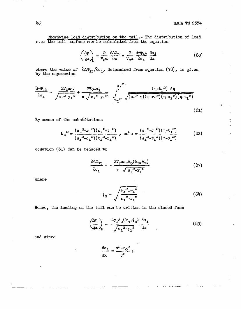
(96)~ ‘~ - ~ j’”~-) Ao2(k4,$,Waq aq

r.

This equation is plotted in figure 4(a) for ro/mco . 0.316.

Chord 10ading.- A closed formula for the loading can be obtained bycarr@ng out the integration ~ (Ap/qa)tdy over the tail or by evaluatingd(~/qa)/clx. However, since the term &( k4,~~) in the expressionfor Ap/qa does not involve y, it is easier to evaluate ~(@/qa)tdy.Thus, using equation (85), the chord loading in the 61 plane is given by

i.

.— — -.——- .————...—-. -—. ...—. —------

49

In the g plane this becomes

(97a)

(97b)

(This checks with the result found by differentiating ~/qa withrespect to x).

Center of pressure.- The center of pressure can be calculatedlymeans of the formula

J

uo/u~gti

rolP axxc.p. = (98)

h

where m/dx is the result just obtained in the previous section~d ~ is given by equation (~). phc@ these ~ues fito

equation (98) yields

xC.p. =9j””~&j$&(k4,y~ti’ (~~)

r.

A graph of this result is shown in figure 5(a) for ro/mcQ= 0.Q6.

, Solution for Rolled Up Vortices

As was.pointed out in the preceding section where the method ofsolution was discussed, the mamner in which the present problem will beattacked is as folldws: First, the velocities induced at the surface ofthe wing and bodyby two point vortices looated somewhere in space willbe calculate% second, a solution wi.11be ~ormulated (by methods identi-cal to those used in part I of this report) that wi12 just cancel thevortex induced velocity component normal to the surface of the wing orbody; third, an additional solution will be formulated that will fit theboundary condtbions prescribed for the tail surface (in this report onlya flat-plate tail surface will be considered).

. . . ... .. . .-. ——— ___________ ______ ..-.__,___ _____ ._ ——. —..— ..._.

50 NACA TN 25s

As usual, it is simpler to work with ‘thetransformed ~1 planethan with the physical ~ plane. Hence, again the Joukowski transfor-mation will.be applied to the field equation and boundary conditions atthe outset of the problem. See sketch (z).

The velocity potential

,i jZ Physical plane at a point (YI,ZI) in the~1 plane induced by a pair ofpoint vortices located at

‘“’fex ‘“c::? ~v;:;; a:’eq$t;:’ ‘s

h Y

“ -i

tJ

rw al (zl-hl)dy=%& =—

~ -al (Y1-Ye)2+(zl-hl)2

[z)

+“+ - (loo)

,iz, Transformed plane where I’w is the strength ofthe cticulation csrried by the

‘Urtex ‘“C’7 ~ P=e18and trailing backfrom the wing tips. The valueof rw/Vo_o that corresponds

h, ~ to the SweptAack wings studied

44

t/ in psrt I of this report is

“q given by equation (32a), thus

—5— 0’ &=2~-(:~]

The values of al and hl depend, of course, on the span of the wing.b order to compare the following results for the rolled up vortices withthose obtained for the sheet vortices in the preceding section, thenumerical results presented in the succeeding examples wilJ.be for

/so mco = 1.7, to/mco /= 1.091, and r. me. = 0.316. ~s pmticularchoice of parameters fixes the span-loading curve for the wing to be thatshown in sketch (o). A reasonable choice for the value of a can becalculated by replacing the figure in sketch (o) bounded by the linesy=ro, I’= o ma the curve for r/Vo~Co by a rectamgle with the sameheight and area. The value of a is then given by the sum of the baselength of this -rectangleand the quantity ro/mco. ~is procedure wascarried out and the result a/mco = 1.545 was obtained. In order toobtain a more complete picture of the effect of the point vortices onthe aerodynamic characteristics of the wing, four different locationswere chosen for the positions ~f the vortices, two in the z=O planefor values of a/mco equal to 1.745 and 1.3, and two at a heighth/mco = 0.3 above the z = O plane for the same two values of a/mco.

.

____ ——— ——— —.—

.

NACA TN 2554 51

From eqmt~ on (100) itccan easily be shown that the value of thevertical induced velocity in the 21 = O plane is

()aqv . r~~[

yl -al Yl+alwv=—

~zl 2==0 1(101) ,

%t h12+(yl-al)2 h12+(yl+al)2

The particular inversion of eqgation (15) thatconditions (see appendfx B) can be written

fits the present boundary

(102)

Place the value of Wv givenby equation (101) into equation (102) amdadd the condition that the tail be a flat-plate lifting surface at anangle of attack u, and there results

J- J-+.Y1-bl yl-bl

.)

(103)

where

bl=al+ihl

:1 = al ~ ihl (104)

and where the radicals are defined uniquely if the complex plane is cut

along the real axis between -m and U=. (For example, G Cwbe set eqml to pleiql where T1 must Me be~een .X ~d ~.)Although the above expression for Av can be ~ut in real terms byapplying the transformations

it is easier in deriving subsequent quantities from Avl to useeqyation (103) first and to make the transformation afterwards.

1

. . . .- ... ._-. ___ ._._ . ___ - ——. .— -.—____ ._ ._ . _

s-pan loading. - The span lomlQ can be determined frcm tiherelation

where Av Is given by equation (103). There fW remiLt6

(lo7a)

(105)

I

~[r12( sinh272-cos2~) +y12] 2+4r12(r12-y12)81&72co~2 -112(B&72 -cos~) -y12 E2< r12 *

t Yl

al Jr12-y12 d-oh 72 COB U2 - 4(Mm) R

I Y

.

.

.

NACA TN 25X 53

The terms sinh 71, SW 72, sin w ~ and sin U2 are all defined in thetable of symbols. $Equations (107a and (107b) can, of course, be trans-formed to the physical plane by transforming each symbol therein fromthe El syst& to the ‘~ system. ‘

—

The variation of the tail span loading, as givenand (10~), is shown in figures 2(a) and 2(b) for thepositions discussed.

fChordWise load distribution.- The loading on thecalculated from the relation

The value

Hence,

of w91t/aU1t follows from equations

dx

by ecyuations(107a)various vortex

tail can be

(108)

(107); thus ‘

‘~--) ] (109)

,

[AP—

Equation (110) when transformed to the ~ plane gives the surface loaddistribution over the tail due to the presence of the two point vorticesas well as the inclination of the tail to the free stream.

Total lift.- The total.lift can be obtained by integrating the spanloading. Thus, if ~ represents the lift oh the tail,

(U-1)

Carrying out this integration yields

Lt.—= fi(al=-rla) - 2W (rl sinh 72 cos 61a-(Y=Sillh71cos Ul)2qa Voa

(1.12)

54 NACA TN 255k..— .

This result was transformed and plotted in figures 3(a) and 3(b) for thevalues discussed.

Total drag.-

where Ft is thesteps (see, e.g.,evaluation of the

a2

2J 1+V2

The final result,

The total drag is given by the relation.

Dt=aLt+Ft (U3)

suction force on the tail leading edge. As in previouseqution (92)) the calculation of Ft depends on thefunction G. ti this case G2 is

ti the ?1 pleme, for the total drag canbe written

Dt

()

rw” 2zn3r(a12-r12)+ A—=

qa2 % v~

(al=-hlz-a=~)2+kl~ l=+(alz-hl=-alz)~(al=-h=z -’wl=)2+hal=hl= ~115)

(alz-hlz-rl=)2&l=hla+( al=-hl=-rl=)~(~z-hl=-rla )2+hal=hl=

Aplot of the drag is given in figures k(a) and k(b).

Chord loading.- As before, in the development of eqwtions (97a)and (97%} for example, the chord loading can be calculated either byperforming the integration .f(Ap/ )t dy, or by differentiatingwith

Trespect to x the total lift (Lt qa). These two different approachesserve to check each other and both lead to the ssme result, namely,

2f”G)t = [’ - V;::d:;::::.l) 1 ‘“’)dy = ‘l’cul~

o

Center of pressure.- Results for the center of pressure XC.p.(where xc.p. = -Mt/Lt) are shown in figures 5(a) and 5(b).

—. . . — .—.

8

.

NACA TN 2554 55

COI?CLUDINGREMARKS

When an airplane is slender enough11 (in the longitudinal sense) oris flying close enough to the speed of sound, the mathematical descrip-

.

tion of its attendant flow field is greatly sin@ified - so much so, infact, that the analysis of whole wing-body-tail conibinationsis feasible.This simplification comes from the fact that the induced velocities ineach lateral plane are completely independent of the nature of we air-plane or flow field behind the reference .plme andare affectedlydisturbances ahead only through the presence of free vortices trailingdo~mstresm from the lifting elements. In the case of a tail, these freevortices stream back from the wing trailing edge.

b thi~ report, speci~ wing plan fbrms were studied: special inthat they produced flat span-loading curves between the wing tips andfuselage. For such wings, the free trailing vortices were concentratedentirely in the region directly behind the wing tips. In general, thetrailing vorticity would be concentrated predominately in this region.The behavior of this trailing vortex system is boundedby the behatiorof two exbreme models: a vortex sheet lying everywhere in the plane ofthe tail, and two laterally symmetric point vortices lytng in or abovethe plane of the tail. Each of these models was e~ned.

One point vortex was placed in the plane of the tail’at a distancefrom the fuselage in the spanwise direction determined by replacing thewing-span loading curve by a rectangle of the same height. As shownbyfigures 2 through 5, the results for this point vortex were not signifi-cantly different from those for the vortex sheet. k either case, thepresence of the trailing wing vortices reducedby about M percent theeffectiveness of the triangular tail surface in producing lift for therange of tail spans and body diameters considered. For the same condi-tions the tail drag was reduced only 18 percent.

For the particular locations chosen for the point vortices, it wasfound that both the lift and drag decreased as the vortices moved closerto the tail. On a percentage basis the decrease was roughly the same.

.,

llThe assumptiotisunderlying slender wing theory are obviously violatedslong lines such as theleading edge, x = mco, and the Mach wave fromthe trailing-edge-fuselagejuncture, x = CO. Along these lines tiepressure gradient is discontinuous and (M&-l] m is not bounded.SWlar situations appear repeatedly in the linearized analysis’ofaerodynamic flotiphenomena and in each case agreement with e~eri-mental results camnok be anticipated.

. . . ..— .. — ..—— .- .—— .—. -

56 NACA TN 2554

.

The position of the center of pressure on the triangular tail wasinsensitive to the presence of the wing vortex system regardless of thevortex pattern chosen. In the extreme case, when the point vortices werenearest the tail, the location of the tail center of pressure with refer-ence to the tail apex as 5 percent forward of the position obtained whenthe wing was absent.

Ames Aeronautical Laboratory~ational Advisory Committee for Aeronautics

Moffett Field, Calif., Aug. 20$ 1951

.

————— — —— — — --

NACA TN 2554 57

a

bl

&

c

co

Cd

cl

d

D

E.

E(k,~)

F

F(k,v)

k

k?

APPENDIX A

LIST’OF ~ORTAIiT SYMBOLS

horizontal distance from y=O plane to(See sketch (z).)

al + ihl

vortex

.

al - ihl

local chord

characteristic chord(See sketch (a).)

()dsection drag coefficient~

()zsection lift coefficientF

section drag force

drag force J

complete elliptic integral of the second kind (~~~d.)

incomplete elliptic integral of the second kind ~-d;

suction force at leading edge of lifting surface.

incomplete elliptic integral of the first kind

(’L*(M&l-t’) )vertical distance from 2=0 plane to vortex

(See sketch (z).)

complete elliptic integral of the first kind

(Jo‘Ji+k5)modulus of elliptic integrals

. . —..-. .- ..—. .——,,..,.. ____ ___ .__________ — --—. --- ——— — ——-–-

58

%

kl

k=

k=

k~

k~

2

L

m

M

%

P

APY

~

r.

s

80

s

t

to

J(s%2-r04)(s2-t2)

t(s2-ro2)

~ in the El plane

2J(S%%04)(S%2)

(s2-ro2)(t2+ro2)

(g)

(a2-ro2)./(s2-t=)(s%~ro4)

(t2-ro2)J (s2-a2)(s2a2-ro4)

section l~t force

lift force

slope of wing leading edge(See sketch (a).)

pitching moment, positive when tail is forced

free-stream Mach number

local static pressure

()P1 -Pllloading coefficient —

q G’ovo’)free-stream dynsmic pressure

radius of boctv(See sketch”

distance from(See sketch

ms2dmm value(See sketc@

wing sxea

distance from(See sketch

maximum value(See sketch

.. — ——

(a). )

x ads to wing leading edge(a).)

of s(a).)

x axis to wing trailing edge(a).)

of t(a).)

— .—. . . . - .——.

NACA TN 255h.

down

)

.

NACA TN 25X “ 59

U,v,w

Au,Av,Aw

Vr

v~

x,y,z

xc.p.’

a

P

Sinh 7=

Sinh 72

r

v

e

%(k, ~)

P

E

P

Po

G

9

AQ

(Aq)T.E.

perturbation velocity coniponentsin the x,y,z directions,respectively

jump @ velocities across 2=0 plane, ~-ul, Vu-vzy wu-wz~respectively

radial comyonent of perturbation velocity in a y,z plane

free-stream velocity

Cartesian coordinates

distance to center of pressure(See sketch (w) and fig. 5.)

angle of attack of airplane

lhll

rlsin~ ,

[1total circulation about wing section (AQ)TOE=

Y2

polar angle in y,z plane

: [m(k’,V) + (E-K)F(k’, $j] .

slope of tail leadihg edge(See sketch (x).)

complex variable (y+iz)

polar distance in y,z plane (JZ2)

free-stream density

distance from x axis to lea&ing edge of tail(See sketch (x).)

perturbation velocity potential

jump in Q across 2=0 tilane

value of A9 at trailing edge

-.-.—— —..-—

(%-%)

------ ... ....-.-.—- —-——-–—-———..— -—-.-

.

60

‘+-=

$7

lffJ

99

siIi2 (q

sin2 w=

1“

12

(13

J(t2+ro2)2 - 4y%2

s(t2+ro2)

t(,92+ro2)

82 2-r.2

s2+ro

s(%-ro2)

t(#-ro2)

plane

plane

plane

plane

(Y)

[ cn2-a12-h12+~(a12+h12-u12)2+ 4U1~12]2012

[r12-a12-h12+~ (a12+h12-r12)2+ 4r12h12]

2rl’=

Subscripts

complex plane resulting from the application of the Joukowskitransformation to

boundary conditions

boundary conditions.

the physical plane

givenby equations (12)

givenby equations (13)

. — — .. —— -— —— ..- ———..- ———

NACA TN 25%61

a

II

1

n

t

u

v.

TT

wake

body

lower surface of 2=0 plane

component normal to leading edge

tail

upper surface of 2=0 plane

rolled up yortex

wing

.

.

. ... . -—. — . .— . ...—--—— ___ .-. .—. .—. .

62 I?ACATN 255h

The integral equation

EQUATION

can be inverted by applying operational techniques. Consider theoperator

(Bl)

.

(B2)

where h(q ~ is a function to be chosen later. Operating On both sidesof equation (Bl) yields

●

where the order of the integral and differential signs Ori‘theright-handside of the equation indicates that tie ~ integration is to be per-formed first.

.

The next step Is to reverse the order of integration in the doubleintegral term in equation (B3). Since am inherent singularity exists inthe area of integration at the point VI = qz . A, however, some caremust be used in order to obtain this reversal. Designating by R(k) thedifference between the term taken firstthen with another, thus

R(x) can be evaluated by isolating thedifference only in its vicinity.. Hence,

with one ord~r of ~tegration and

(nl-11.d(ml)

(B4)

studying the

,_ —...———.—..—— .—. —..-—— —— -—— —-— -— -.. --..-—--————- —

9

L+E ?&s

63

(B5)

Using the transformations ql = A-exl and 72 = k-ex2, equation (B5)can be reduced to the form

f= 2Av(k)h(x)

l-xl1&L2n—0 xl 1+X1

=-~Av(A)h(k) (1%)

Substitute equations (B6) and (B4) into equation (B3) and thereresults

or

If

Av(x) =

h(~l) = ~(b-~l )(~l-a) equation (B7) becomes

N’.J&- $ abAv(q2)dq2

1

(B8)

Since, however, equation (38) contains both & an. its integral, itdoes not represen{ a uni~e solution for A.. In order to obtati”aunique solution, some additional.condition must be imposed. If thiscondition is that A.(a) = O, then the proper choice of h(~) in equa-

. tion (B7) is

. ..— .. ...-. —--— .- .-. . — .-— ..— —--—- ——-— -— --- —--. .——— -- -.. - ——.—.—.-

— ——-.

64

which leads immediately to the unique result

.

(B9)

.

.

-——-- —.

(,’

NACA TN 2554 .65

lwFERENcEs

1. Jones, R. T.: Properties of Low-Aspect-Ratio Pointed Wings at SpeedsBelow smd Above the Speed of Sound. NACA Rep. 835, 1946. (For-merly NACA TN 1032)

2. Heaslet, Max. A., Lomax, Hsrvard, and Spreiter, John R.: LinearizedCompressible-FlowTheory for Sonic Flight Speeds.NACA Rep. 956, 1950. (Formerly NACA TN 1824)

3. Spreiter, JobR.: Aerodynamic Properties of Slender Wing-BodyCombinations at Subsonic, Transonic, and Supersonic ,@eeds.NACA Rep. 962, 1948. (Formerly NACATN’s 1662 and 1897)

4. Lomaxj Harvard, and Heaslet, Max. A.: Linearized Lifting-SurfaceTheory for Swept-Back Wings with Slender Plan Forms.NACATN 1992, 1949.

~. Heaslet, Max. A., andhmax, Harvard: The Application of GreentsTheorem to the Solution of Boundary-Value Problems in LinearizedSupersonic Wing Theory. NACA Rep. 961, 1950. (FormerlyNACA TN1767)

6. Cohen, Doris: The Theoretical Lift of Flat Swept-Back Wings atSupersonic Speeds. NACATN 1555, 1948.

7. Cohen, Doris: Theoretical Loading at Supersonic Speeds of FlatSwept-Back Wings with Interacting Trailing and Leading Edges.NACA TN 1991, 1949.

8. Bro~m, Clinton E.: Theoretical.Lift and Drag of Thin TriangularWings at Supersonic Speeds. NACARep. 839, 1946.

9. Heuman, Carl: Tables of Complete.Elliptic Integrals. Journal ofMathematics and Physics, v. 20, 1941, pp. u7-206.- .

10. Spreiter, John R.,and Sacks, Alvin H.: The Rolling UQ of the Trail-ing Vo&kx Sheet and itsJour. of the Aero. Sci.,

fifect on the DownWash Behind Wings.vol. 18, January 1951, pp: a-32.

, t

. .. . ... . .. .—— ——. —.-e.—. — . ..— — - —-—— . ..- .-— .— -— —-.. .- . . ..— ..-

66

ro/mco=

x/co1.001.051.101.15

1.201.301.401.50

1.601.802.002.20

2.603.003.504.00

0

y/mco

o.168.256.332

.400

.526

.644

.756

.8671.0831.2971.507

1.912.322.833.33

NACA TN 259.

TABLE I.- POSITIOI?OF TRAILING EOGE

).100 0.224

~~mcoy/mco

).100 0.224.213 .323.290 .387.361 .447

.425 -.504

.545 .614

.661 .7ZL●773 .826

.884 .931L.096 1.140

L.308 1.394L.516 1.555

L.92 1.96?.33 2.37?.84 2.873.34 3.38

J.316 0.447 0.500

yim~o yimco yimco

2.31-60.447 0.500● 413 .542 .593X& .598 .649

.648 .699

.57’9 .698 .748

.682 .797 .845

.786 .896 .941

.888 .993 1.036

.990 1.090 1.130L.192 1.283 1.323L.393 1.482 1.522L.596 1.676 1.723

?.00 2.07 2.122.40 2.47 2.522.91 2.98 3.02

3“41- 3.49 3.52

0.600

y/mco

0.600.690.746.796

.845

.9411.0331.I_28

1.2221.4131.6101.803

2.202.603.103.60

Iy/mco y/mco

0.700 0.800.791 .883.844 .933.890 .982

.933 1.0311.028 1.1261.123 1.2211.217 1.315

1.312 1.4121.504 1.6061.700 1.8001.893 1.996

2.29 2.392.69 2.793.19 3.293.69 3.78

0.900

y/mco

0.900.970

1.0201.067

1.1131.213I. 3121.410

1.5061.7031.8002.100

2.502.903.393.89

— —.-— ..— —,. .

NACA TN 25% 67

r/mco=

y/lllc~

o.100.227.316.447.500.600.700.8●9

1.0

1.1

1.21.31.41.61.82.02.53.04.0

0

c/co

L.000.926.910.826.790.777.760.748.738.728.722.719.708.703.699.692.687.682.674.669.660

TABLE II.- VALLJESOF LOCAL CHORD

0.100

C[co--b

0.900.8u.802.772.761.746●735.724.715.709.704.697.692.688.682.677.672.663.65(.648

).224

:/co

------

). 776.732.703.695.685.679.673.668.665.661.659.653.651.645.642.639.631.625.613

J. 316

,/co

------

;. ;8~.633.627.620.617.614.612.610.608.607.606.605.603.601●599.595.593.392

0.447 0.500

Cjco c/co

--- ------ ------ ------ ---

0.553 ---.522 O.y)o.504 .462.498 .451.500 .452.503 .b59.505 .464,508 .468.512 :::.515.518 .477.522 .480.524 .481.525 .482

.522 .484

.519 .485

.514 .485

).600

:/co

------------------

).400.362● 355● 3%.365.372

..376.381.385.392.396.398.403.406.410

---------------------

). 300.262.260.269.278.285.290.294.299.302.305.311.315.318

1.800

------------------------

).200.170.170.175.180.185.189.196.200.204.212.218.225

) .900

:/co

---------------------------

)● 100● 082.079.081.087.094.o$13.100.100.101.102.102

—-. ------ .—. -.————-- ---— __ . .. .

.—-— — . . ...— .— .

.

B

.. .———. —— . .— —- ——. . —. .—..— ..—. —-..-——— ..—. —._—._ .—.—..

69

0#o / O*

(a) Gonstont f. /mce

Figure 1.- Re]otions between the wing area, wing spaq ondbody diometer.

. . . .—. --—. .--—..-. .— -— —-—.—.- —..——--- —— -.. ...— ----— .. . . ... . . ----- --

———. .———

70

8

7

6

5’

s~:

4

3

2

I

0

NACA TN 255k

\

S represents oresof wing ponelsonly

\

\

\I

1

\

\

—

o .2 4 .6 .8 i.o~/sO

(b} Constant ~/s. .

Figure i.- Concluded. .

.

__ .——-——.. —. ——. .

—.. . —*o

.8

.4.

0 .2 ‘6 y/mcO .8/.0 1.4

[o) Vortex sheet.

Figure i?. - Voriotion of the span loading on the toll.

‘d

I

,

I

I“o .2 .4 .6 .8 10 1.2

y/m co

(b~ ?olnt vortices.

I

Figure 2.- Concluded.

I

r

NACA TN 25A 73

.

.4

.3

L,

43

.2

.)

t

/Vortex sheet — /

Rolled upvortices

-------- (

[~=o I

o/mco = /. 545)

No wing —-—/

G/me,, = .316/

/

/

.2 4 .6 .8 10O#m co

(a) Vortex sheet.

.3 I I IVortex positions

I I I /

.2

L,

4qd.#

./~/mco= .316

I

.2 # .8 lo~.?m~

lbj Point vortices.Figure 3.- Voriotion of the lift on the toil.

.. . .. .. . . . . . . ... . . . . . . . . . . . --- ... . ........ . . . . . . . . . --- ./

_—— —. —. ._

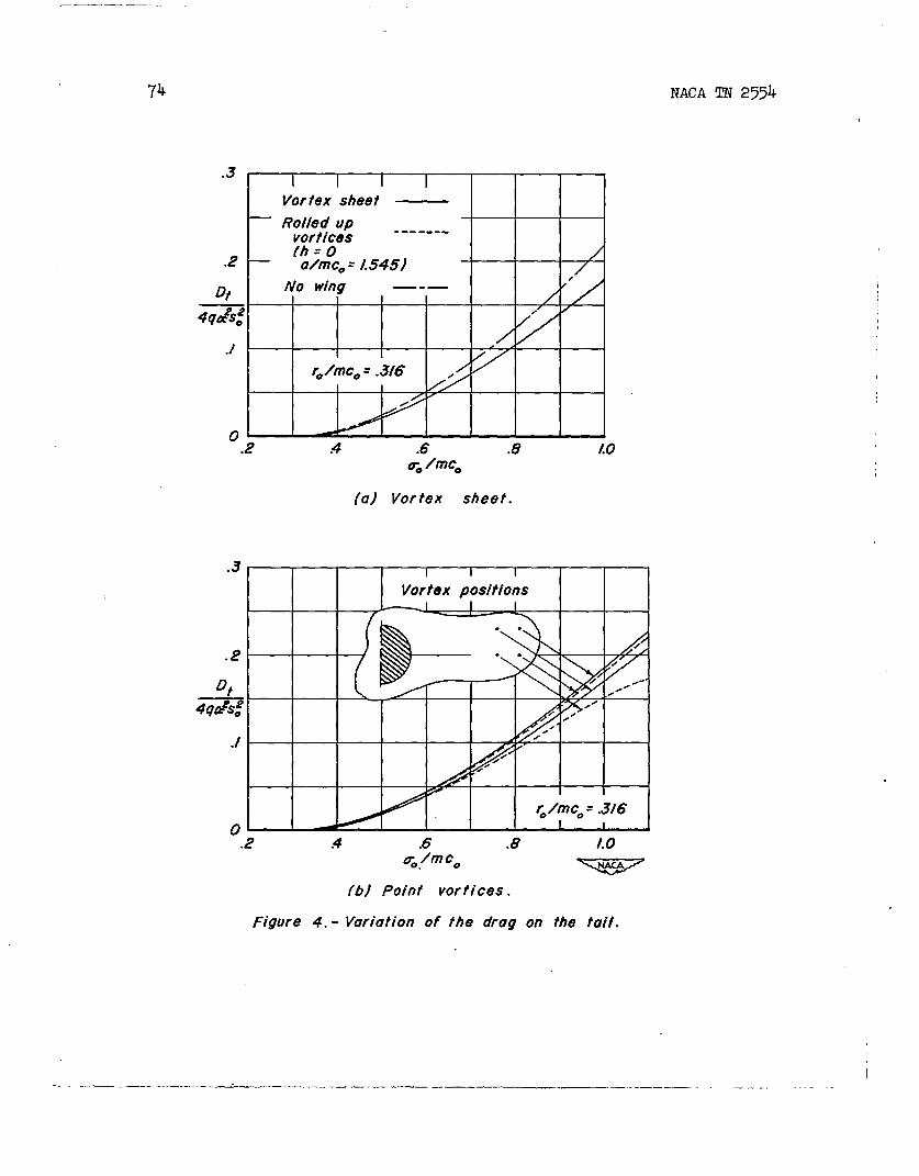
74

Vortex sheet —

— Rolled up .---..-vortices

.2(h=O /o/mcO = 1.545) /

No wing/

Dt—-—

4qC&:

./

re/mcO = .3/6 //

n.2 .4 .6 .8 10

~. /mee

(a) Vortex sheet.

.3

o.2 .4 .6 .8 /.0

Figure 4.-

rO./m co

[b) Point vortices.

Variation of the drag on the toil.

-.—. —__ ———= — ___ ..——__ —.. .

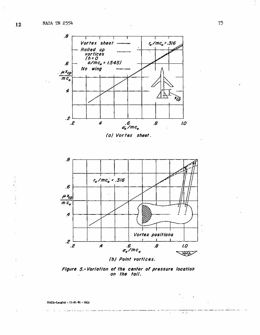
12 NACA TN 75

I I I I I I I IVortex sheet — ~Ance=.3/6

— Rolled up ------- “ .vortices(h=O

.6No wing —-—

. Pxcp~

4

.2.2 4 .6 .8 10C*/nlc*

(a) Vof tex Sheet .. .

/’ 1r’ /mco” =. 316

/ 1~l!

“ w

II. .

.0

II I Vortex positions I

.4 .6 .8~O/mcO

[b) Point vortices.&

Figure 5.-Variation of the center of pressure locationon the toil.

NACA-Lan@y -11-.91-61-1000

..-. . . .. .. -. ————-. - -T .. —.. .— .—. ..- --

. .,