Embed Size (px)
Citation preview

Quantum Field Theory I
Christof Wetterich
August 8, 2006
This is a script to Prof. Wetterich’s QFT I lecture at theuniversity of Heidelberg in the winter semester 2005/06.The latest version can be found at the course homepagehttp://www.thphys.uni-heidelberg.de/~cosmo/view/Main/QFTWetterich.
If you find an error, please check whether you have the newest version (seedate above), and if so report it to [email protected]. Also if you findsomething confusing and think it should be explained in more detail or moreclearly, please let us know. Your feedback will be the main force to improve thescript.
The Quantumfive are:Christoph Deil, Thorsten Schult, Dominik Schleicher, Simon Lenz, Gerald

2

Contents
1 Quantum Fields 7
1.1 Introduction . . . . . . . . . . . . . . . . . . . . . . . . . . . . . . . . . . . 7
1.2 Units . . . . . . . . . . . . . . . . . . . . . . . . . . . . . . . . . . . . . . . 7
1.3 Non-Relativistic Many-Body Systems 1: Phonons . . . . . . . . . . . . . . 8
1.3.1 One Dimensional Crystal . . . . . . . . . . . . . . . . . . . . . . . 8
1.3.2 Propagating Phonons . . . . . . . . . . . . . . . . . . . . . . . . . 11
1.3.3 Block Diagonalization . . . . . . . . . . . . . . . . . . . . . . . . . 14
1.3.4 One Dimensional Phonons . . . . . . . . . . . . . . . . . . . . . . . 15
1.3.5 Summary . . . . . . . . . . . . . . . . . . . . . . . . . . . . . . . . 16
1.3.6 The Symplectic Group Sp(V ) . . . . . . . . . . . . . . . . . . . . . 16
1.3.7 Further Discussion of Phonons . . . . . . . . . . . . . . . . . . . . 17
1.4 Non-Relativistic Many-Body Systems 2: Atom Gas . . . . . . . . . . . . . 24
1.4.1 Identical Bosonic Atoms in a Box . . . . . . . . . . . . . . . . . . . 24
1.4.2 N -Atom States . . . . . . . . . . . . . . . . . . . . . . . . . . . . . 26
1.4.3 Continuum Limit . . . . . . . . . . . . . . . . . . . . . . . . . . . . 27
1.4.4 Quantum Fields - Summary . . . . . . . . . . . . . . . . . . . . . . 29
1.4.5 Atom Gas . . . . . . . . . . . . . . . . . . . . . . . . . . . . . . . . 30
1.4.6 From Quantum Field Theory to Quantum Mechanics for a One-Atom State . . . . . . . . . . . . . . . . . . . . . . . . . . . . . . . 31
1.4.7 Heisenberg Picture for Field Operators . . . . . . . . . . . . . . . . 32
1.4.8 Field Equation for φ(x, t) . . . . . . . . . . . . . . . . . . . . . . . 33
1.5 Correlation Functions, Propagator . . . . . . . . . . . . . . . . . . . . . . 34
1.5.1 One Particle States . . . . . . . . . . . . . . . . . . . . . . . . . . . 34
1.5.2 Transition Amplitude . . . . . . . . . . . . . . . . . . . . . . . . . 35
1.5.3 Completeness . . . . . . . . . . . . . . . . . . . . . . . . . . . . . . 36
1.5.4 Huygens Principle . . . . . . . . . . . . . . . . . . . . . . . . . . . 36
1.5.5 The Propagator G . . . . . . . . . . . . . . . . . . . . . . . . . . . 36
1.5.6 Free Non-Relativistic Propagator . . . . . . . . . . . . . . . . . . . 36
1.5.7 Time Dependence . . . . . . . . . . . . . . . . . . . . . . . . . . . 39
1.5.8 Higher Correlation Functions . . . . . . . . . . . . . . . . . . . . . 40
1.5.9 Time Ordered Correlation Functions . . . . . . . . . . . . . . . . . 40
1.5.10 Time Ordered Two-Point Function . . . . . . . . . . . . . . . . . . 41
3

Contents
2 Path Integrals 432.1 Path Integral for a Particle in a Potential . . . . . . . . . . . . . . . . . . 43
2.1.1 Basis of Eigenstates . . . . . . . . . . . . . . . . . . . . . . . . . . 432.1.2 Transition Amplitude . . . . . . . . . . . . . . . . . . . . . . . . . 44
2.1.3 Infinitesimal Transition Amplitude . . . . . . . . . . . . . . . . . . 452.1.4 Split of Amplitudes in Product of Infinitesimal Amplitudes . . . . 462.1.5 Path Integral . . . . . . . . . . . . . . . . . . . . . . . . . . . . . . 47
2.1.6 Action . . . . . . . . . . . . . . . . . . . . . . . . . . . . . . . . . . 482.1.7 Interpretation of QM, Double Slit Experiment . . . . . . . . . . . 50
2.1.8 Classical Path . . . . . . . . . . . . . . . . . . . . . . . . . . . . . . 512.1.9 Operators . . . . . . . . . . . . . . . . . . . . . . . . . . . . . . . . 53
2.1.10 Can One Construct QM from a Path Integral? . . . . . . . . . . . 542.1.11 Generalization to N Degrees of Freedom . . . . . . . . . . . . . . . 55
2.2 Functional Integral for Bosonic Many-Body Systems . . . . . . . . . . . . 55
2.2.1 Path Integral for QFT . . . . . . . . . . . . . . . . . . . . . . . . . 552.2.2 Systems in Various Dimensions d . . . . . . . . . . . . . . . . . . . 58
2.2.3 In and Out States . . . . . . . . . . . . . . . . . . . . . . . . . . . 582.2.4 S-Matrix . . . . . . . . . . . . . . . . . . . . . . . . . . . . . . . . 59
2.2.5 Functional Integral for the S-Matrix . . . . . . . . . . . . . . . . . 592.2.6 Correlation Function . . . . . . . . . . . . . . . . . . . . . . . . . . 612.2.7 Two-Point Function in Free Theory . . . . . . . . . . . . . . . . . 62
2.2.8 S-Matrix Element in One-Particle Channel . . . . . . . . . . . . . 642.2.9 Reduced Transition Amplitude M . . . . . . . . . . . . . . . . . . 64
2.2.10 Classical Approximation for 2 → 2 Scattering . . . . . . . . . . . . 652.3 Generating Functionals . . . . . . . . . . . . . . . . . . . . . . . . . . . . . 74
3 Fermions 773.1 Fermionic Quantum Fields . . . . . . . . . . . . . . . . . . . . . . . . . . . 77
3.1.1 Pauli Principle . . . . . . . . . . . . . . . . . . . . . . . . . . . . . 773.1.2 Symmetries and Normalization of N -Fermion States . . . . . . . . 773.1.3 Annihilation and Creation Operators . . . . . . . . . . . . . . . . . 78
3.1.4 Occupation Number, Hamiltonian . . . . . . . . . . . . . . . . . . 793.1.5 Fermion Field . . . . . . . . . . . . . . . . . . . . . . . . . . . . . . 80
3.2 Path Integral for Fermionic Systems, Grassmann Variables . . . . . . . . . 803.2.1 Several Grassmann Variables . . . . . . . . . . . . . . . . . . . . . 82
3.2.2 Functions of Grassmann Variables . . . . . . . . . . . . . . . . . . 843.2.3 Differentiation . . . . . . . . . . . . . . . . . . . . . . . . . . . . . 853.2.4 Integration . . . . . . . . . . . . . . . . . . . . . . . . . . . . . . . 87
3.3 Functional integral with Grassmann variables . . . . . . . . . . . . . . . . 873.3.1 Partition function . . . . . . . . . . . . . . . . . . . . . . . . . . . 87
3.3.2 Correlation functions . . . . . . . . . . . . . . . . . . . . . . . . . . 883.3.3 Simple Grassmann integrals . . . . . . . . . . . . . . . . . . . . . . 89
3.3.4 Free Green’s function for non-relativistic fermions . . . . . . . . . 903.4 Functional integral for fermionic quantum systems . . . . . . . . . . . . . 90
4

Contents
3.4.1 Correlation functions . . . . . . . . . . . . . . . . . . . . . . . . . . 90
4 Relativistic Quantum Fields 914.1 Lorentz Transformations . . . . . . . . . . . . . . . . . . . . . . . . . . . . 91
4.1.1 Lorentz Group and Invariant Tensors . . . . . . . . . . . . . . . . . 914.1.2 Lorentz Group . . . . . . . . . . . . . . . . . . . . . . . . . . . . . 944.1.3 Generators and Lorentz Algebra . . . . . . . . . . . . . . . . . . . 964.1.4 Representations of the Lorentz Group (Algebra) . . . . . . . . . . 1004.1.5 Transformation of Fields . . . . . . . . . . . . . . . . . . . . . . . . 1014.1.6 Invariant Action . . . . . . . . . . . . . . . . . . . . . . . . . . . . 1034.1.7 Functional Integral, Correlation Functions . . . . . . . . . . . . . . 104
4.2 Dirac Spinors, Weyl Spinors . . . . . . . . . . . . . . . . . . . . . . . . . . 1054.2.1 Spinor Representations of the Lorentz Group . . . . . . . . . . . . 1054.2.2 Dirac Spinors . . . . . . . . . . . . . . . . . . . . . . . . . . . . . . 1064.2.3 Weyl Spinors . . . . . . . . . . . . . . . . . . . . . . . . . . . . . . 1084.2.4 Dirac Matrices . . . . . . . . . . . . . . . . . . . . . . . . . . . . . 109
4.3 Free Relativistic Fermions . . . . . . . . . . . . . . . . . . . . . . . . . . . 1104.3.1 Invariant Action . . . . . . . . . . . . . . . . . . . . . . . . . . . . 1104.3.2 Transformation of Spinor Bilinears . . . . . . . . . . . . . . . . . . 1114.3.3 Dirac Spinors with Mass . . . . . . . . . . . . . . . . . . . . . . . . 1124.3.4 Dirac Propagator . . . . . . . . . . . . . . . . . . . . . . . . . . . . 118
4.4 Scalar Field Theory . . . . . . . . . . . . . . . . . . . . . . . . . . . . . . 1194.4.1 Charged Scalar Fields . . . . . . . . . . . . . . . . . . . . . . . . . 1194.4.2 Feynman Propagator . . . . . . . . . . . . . . . . . . . . . . . . . . 1204.4.3 Particles and Antiparticles . . . . . . . . . . . . . . . . . . . . . . 1214.4.4 In- and Out Fields . . . . . . . . . . . . . . . . . . . . . . . . . . . 122
5 Scattering and decay 1235.1 S-Matrix and Greens-Functions . . . . . . . . . . . . . . . . . . . . . . . . 123
5.1.1 Scattering amplitude for relativistic charged scalar field . . . . . . 1235.1.2 The LSZ Formalism . . . . . . . . . . . . . . . . . . . . . . . . . . 123
5.2 Scattering and decay . . . . . . . . . . . . . . . . . . . . . . . . . . . . . . 1245.2.1 Differential cross section . . . . . . . . . . . . . . . . . . . . . . . . 1245.2.2 Lorentz covariant building blocks . . . . . . . . . . . . . . . . . . . 1245.2.3 Tree scattering in scalar theory . . . . . . . . . . . . . . . . . . . . 1245.2.4 Generalizations . . . . . . . . . . . . . . . . . . . . . . . . . . . . . 1245.2.5 Point like Interaction of Non-relativistic Spinless Atoms . . . . . . 1265.2.6 Point like Interaction of Non-relativistic Atoms with Spin 1/2 . . . 1275.2.7 Relativistic Dirac Particles: Normalization and On Shell Condition 128
5.3 Solutions of free Dirac equation . . . . . . . . . . . . . . . . . . . . . . . . 1355.3.1 Basis spinors in rest frame . . . . . . . . . . . . . . . . . . . . . . . 1365.3.2 General decomposition of Dirac Spinor . . . . . . . . . . . . . . . . 1385.3.3 Reduced matrix element and scattering . . . . . . . . . . . . . . . 1395.3.4 Basis spinors for arbitrary momentum . . . . . . . . . . . . . . . . 139
5

Contents
6
1 Quantum Fields
1.1 Introduction
Quantum field theory (QFT) is a theory that is useful not only for elementary particlephysics, but also for understanding certain aspects of e.g. atoms, gases or solids. Onecan say that
QFT is quantum mechanics (QM) for systems with many (sometimes in-finitely many) degrees of freedom.
QFT is conceptually not beyond QM. But the large number of degrees of freedom createqualitatively new effects. The relationship between QFT and QM is similar to therelationship between statistical mechanics and mechanics.
The basic problem of QFT is how to treat these infinitely many degrees offreedom.
A good theory should be independent of how exactly this limit process is done.One topic in QFT is the renormalization group. It is concerned with the question of
how to translate microscopic, short distance laws to larger systems. Only part of theinformation is appearing on larger scales.
The key method to make QFT simple is functional integrals. We will however startwith the more familiar creation/annihilation operators in this chapter and then move onto functional integrals in chapter 2.
1.2 Units
We use units in which
~ = c = 1. (1.1)
From c = 1 it follows that 1 s = 299792458m and that mass and energy have the sameunits (E = mc2). We measure mass and energy in eV. The mass of an electron is there-fore me = 510 998.902(12) eV ≈ 9.1 · 10−31 kg. Obviously, velocities are dimensionless.Momentum is therefore also measured in eV.
¿From ~ = 1 it follows that the unit of length is the inverse of the unit of energy.Knowing that ~c ≈ 197GeV m in the SI system we can easily convert between units, forexample:
1 fm = 10−15 m =1
197MeV≈ 5GeV−1
1Hz = 1 s−1 = 6.66 · 10−16 eV (1.2)
7

1 Quantum Fields
As an example of how our new units make life simple consider the commutator rela-tion between the position operator Q and the momentum operator P , which used to be[Q,P ] = i~ and now simply is [Q,P ] = i, i.e. QP is dimensionless.
Exercise: Express the Bohr radius a0 ≈ 0.5 · 10−10 m in eV−1.
1.3 Non-Relativistic Many-Body Systems 1: Phonons
We will treat these systems now with the so called operator formalism, which is alsocalled canonical quantization, because students already know this method from QM. Inchapter 2 we will do the same problem again with a new, better method called functionalformalism.
1.3.1 One Dimensional Crystal
The reason why we start with this system is that all the basic concepts of QFT arealready present here. Doing it in three dimensions would only increase the number ofindices and give nothing conceptually new.
We consider a one dimensional lattice with N lattice sites (N even) and one atomat every lattice site j. For simplicity we connect the lattice to a torus and identifyN/2 with −N/2. For large N that is physically the same as the linear lattice, but ismathematically more simple because there are no boundaries.
Let Qj be the displacement from the equilibrium position and Pj the momentum ofthe atom at lattice site j. Then we have the following commutator relations:
[Qi, Pj ] = iδij ,
[Qi, Qj ] = 0,
[Pi, Pj ] = 0. (1.3)
They express that different atoms are completely independent, but position and momen-tum of one particle are related.
As a first dynamical model for our crystal we treat the atoms as independent harmonicoscillators. This is described by the simple Hamiltonian
H0 =∑
j
(D
2QjQj +
1
2MPjPj
)(1.4)
which has N degrees of freedom and no interaction between lattice sites. To solve thisproblem we define for each lattice site j two operators which are linear combinations ofthe position and the momentum operator of that site:
annihilation operator : aj =1√2
((DM)
14Qj + i(DM)−
14Pj
),
creation operator : a†j =1√2
((DM)
14Qj − i(DM)−
14Pj
). (1.5)
8

1.3 Non-Relativistic Many-Body Systems 1: Phonons
The fact that a†j is the adjoint of aj, i.e. that a†j = (aj)†, justifies the notation a†j. These
operators satisfy the following relations:
[ai, a†j ] = δij ,
[ai, aj ] = 0,
[a†i , a†j ] = 0. (1.6)
We can express the Hamiltonian in terms of the annihilation and creation operators:
H0 = ω0
∑
j
(a†jaj +1
2) = ω0
∑
j
a†jaj +N2ω0,
where ω0 : =√D/M. (1.7)
For N → ∞, the second term in the Hamiltonian goes to infinity. However, this di-vergence is not problematic, since we measure only differences in energy and the pointof zero energy is a matter of definition. We simply subtract the term to get the rightresult. But this is a phenomenon we will encounter quite often in QFT and we alwayshave to make sure that the divergent terms are not connected to observable quantities,otherwise we will be in trouble.
Occupation Number Representation
A basis vector in the occupation number representation contains for each possible stateof a system the number of particles that occupy it. We can describe the state |Ψ〉 in theoccupation number basis by
|Ψ〉 = |n−N2, . . . , n−1, n0, n1, . . . , nN
2−1〉. (1.8)
The particle number operator for the lattice site j can be expressed as
nj = a†jaj. (1.9)
It counts the number of phonons at lattice side j
nj| . . . , nj, . . . 〉 = nj| . . . , nj, . . . 〉. (1.10)
The total occupation number operator is given by
N =∑
j
nj . (1.11)
Note the different meaning of N and N :
N = number of degrees of freedom of the system (here the number of lattice sites)
N = total number of excitations in the system (here the number of phonons)
9

1 Quantum Fields
QFT deals with large N , not necessarily with large N . For example QFT can de-scribe phonon-phonon scattering in a crystal. There you have N ≈ 1023 and N = 2.The situation is similar for processes like electron-photon or electron-electron scattering.They involve only N = 2 particles (particles are described as excitations of the vacuum),but N = ∞ degrees of freedom, namely the possible momenta of the outgoing particles.Even the ground state |0〉, where N = 0, is often a very complicated object in QFT!
N can be large too in QFT, e.g. if you want to describe a cold atom gas you can easilyhave N ≈ 105. But the important characteristic of all systems studied in QFT is thatthey have very many degrees of freedom.
Basic Concepts of QFT
By now we have already met all the basic concepts of QFT:
vacuum = ground state: We call the ground state of our world the vacuum. The vac-uum state |0〉 = |0, 0, 0, . . . , 0, . . . , 0〉 is a normalized state in Hilbert space. It isthe state of lowest energy, not necessarily zero energy. |0〉 6= 0, the vacuum is notempty, it can be very complicated.
particles = excitations of ground state: The excitations of the ground state are theparticles. Particle properties depend on the ground state. For a solid that isobvious, the phonons depend on D and M . But for any system they depend onthe Hamiltonian.
• 〈nj〉 = 0.3 says that the expectation value of finding a phonon at site j is 0.3
• If a state has a sharp number of nj phonons at site j then the equationnj|Ψ〉 = nj|Ψ〉 says that |Ψ〉 is a superposition of states | . . . , nj, . . . 〉 whichall have nj atoms at site j.
operator fields: We have a field of operators aj ≡ a(j) ≡ a(x) with x = j · a (a de-notes the distance between adjacent lattice sites). That is a new concept, e.g. inelectrodynamics of quantum mechanics we just dealt with scalar of vector fields.You can’t measure these operators because they are not Hermitian, but Hermitianfields are easily constructed from a(x) and a†(x):
q(x) =1√2
(a(x) + a†(x)
)= (DM)
14Q(x),
p(x) = − i√2
(a(x) − a†(x)
)= (DM)−
14P (x) (1.12)
are observables with real expectation values and [qi, pj ] = iδij .
QFT is conceptually very simple, but it is technically difficult because the Hamiltoniansdescribing real physical systems are complicated.
10

1.3 Non-Relativistic Many-Body Systems 1: Phonons
1.3.2 Propagating Phonons
So far our “phonons” are quite boring: Eigenstates of H0 are confined to a given latticesite. Each lattice site can be treated independently of other sites. It is only a collection ofone particle systems, we need interaction between lattice sites for propagation. Thereforewe introduce next neighbor interaction into our Hamiltonian.
H = H0 +Hnn,
Hnn = −B2
∑
j
Qj+1Qj = −B4
∑
j
(Qj+1Qj +Qj−1Qj) (1.13)
Now we have coupled oscillators! We consider B > 0 so the “alignment” of Qj is favoredbecause it needs less energy. The solution is still simple because this is a linear system.The diagonalization of H is possible.
Classical System
We will setup and solve the equations of motion for the classical system. The equationsare
Qj =1
MPj ,
Pj = − ∂H
∂Qj. (1.14)
The equation of motion is given by
MQj = −DQj +B
2(Qj+1 +Qj−1) (1.15)
and the Fourier transform of Qj is
Fq =∑
j
e−iqajQj . (1.16)
Here we used the same definitions as already introduced in chapter 1.3.1. a is theperiodicity constant of our lattice such that a · j = x is the continuous spacial variable.The classical momentum is q. Inserting the Fourier transform into the equation of motiongives
MFq =∑
j
e−iqaj(−DQj +B
2(Qj+1 +Qj−1))
= −D∑
j
e−iaqjQj −B
2
∑
j
e−iqa(j−1)Qj −B
2
∑
j
e−iqa(j+1)Qj
= −∑
j
e−iqajQjD − B
2(eiqa + e−iqa) = −Fq · (D −B cos qa). (1.17)
This equation is solvable with the ansatz
Fq(t) = eiωqtFq1 + e−iωqtFq2, where ω2q =
D −B cos qa
Mand |B| ≤ D. (1.18)
11

1 Quantum Fields
Quantum System
For the quantum system, we need to make a finite Fourier transform. This gives us thecreation and annihilation operator of a wave mode (phonon) with momentum q:
aq =1√N∑
j
e−iqajaj ,
a†q =1√N∑
j
eiqaja†j . (1.19)
Note that this isn’t the Fourier transform of the momenta Pj and the space variablesQj . We are interested in the momentum properties of a discrete torus lattice. Thecircumference is L = aN , the longest wavelength possible is L/2 and the shortest is2a. Thus the momenta are q = 2π kL , where all integers k =, 0,±1,±2,±3, . . . ,±N
2 arepossible. One finds the periodicity in j
e−iqa(j+N ) = e−iqaj (1.20)
and the periodicity in q
q′ = q +2π
a→ aq′ = aq → identify q and q +
2π
ak. (1.21)
Let’s calculate the commutator of a†q and aq′ :
a†qaq′ =1
N∑
j
∑
j′
eia(qj−q′j′)a†jaj′
aq′a†q =
1
N∑
j
∑
j′
eia(qj−q′j′)aj′a
†j ,
[aq′ , a†q] =
1
N∑
jj′
eia(qj−q′j′)[aj′ , a
†j ] (1.22)
We know that [aj′ , a†j ] = δj′j and thus we have (m integer)
[aq′ , a†q] =
1
N∑
j
eiaj(q−q′) = δ(q − q′) =
1 for q′ = q + 2mqmax where qmax = π
a
0 otherwise.
(1.23)
Proof: A useful identity is 1N∑
j e2πiNkj = δk,0 for: j, k integer, |j| ≤ N
2 ,
j = ±N2 identified, N even, δk,0 = 1 for k = 0 modN , 0 otherwise.
The number operator for a phonon in q-mode is given by nq = a†qaq, with the conditions
−πa ≤ q ≤ π
a , with −πa and π
a identified (momenta on torus!). It follows that [aq, a†q] = 1
and that all other commutators vanish.
12

1.3 Non-Relativistic Many-Body Systems 1: Phonons
The inverse finite Fourier transformation is given by
aj =1√N∑
q
eiaqjaq
with
∑
q
=∑
|q|≤πa
=∑
|k|≤kmax=∑
|k|≤N2
(1.24)
Proof: Insert the definition of aq.
We now want to express Hnn in terms of aq and a†q:
Hnn = −B2
∑
j
Qj+1Qj,
Qj =1√2(DM)−
14 (aj + a†j),
⇒ Hnn = −B2
(DM)−1/2
2
∑
j
(aj+1 + a†j+1)(aj + a†j). (1.25)
Setting β = B(DM)−1/2
4 gives
Hnn = −∑
j
∑
qq′
β
N (eiaq(j+1)aq + e−iaq(j+1)a†q)(eiaq′jaq′ + e−iaq
′ja†q′) (1.26)
replace q by −q for a†, this is just rearranging the sums
Hnn = − β
N∑
qq′
∑
j
eia(q(j+1)+q′j)(aq + a†−q)(aq′ + a†−q′)
= − β
N∑
qq′
eiaq∑
j
eia(q+q′)j(aq + a†−q)(aq′ + a†−q′). (1.27)
Using formula (1.23)∑
j eia(q+q′)j = N δq,−q′ we get
Hnn = −β∑
q
eiaq(aq + a†−q)(a−q + a†q) (1.28)
With aq, a†q′ = a†q′aq + δq,q′ one finds
Hnn = −β∑
q
eiaq(a†−qa−q + a†qaq + 1 + aqa−q + a†qa†−q). (1.29)
13

1 Quantum Fields
With∑
q eiaq = 0 follows
Hnn = −β∑
q
(eiaq + e−iaq)a†qaq +1
2(aqa−q + a†qa
†−q),
= −B(DM)−1/2
2
∑
q
cos aqa†qaq +1
2(aqa−q + a†qa
†−q), (1.30)
H0 =
√D
M
∑
j
a†jaj =
√D
M
∑
q
a†qaq. (1.31)
Proof: The reader should verify this!
The general Hamiltonian H is then given by
H = H0 +Hnn =
√D
M
∑
q
hq,
hq = (1 − B
2Dcos aq)a†qaq −
B
4Dcos aq(aqa−q + a†qa
†−q). (1.32)
As we now see, H separates into contributions from individual |q| modes, but it still
mixes between aq and a†−q!
1.3.3 Block Diagonalization
Until now, we have been able to decompose all modes of H, with different |q|. Todecompose the terms with q and −q, we introduce new operators Aq and A−q for α, β ∈ R
via
aq = αAq + βA†−q, a†q = αA†
q + βA−q,
a−q = αA−q + βA†q, a†−q = αA†
−q + βAq. (1.33)
At first glance, one assumes, that this is an orthogonal transformation, but we’ll seeit’s NOT. The reason is, that we would like the algebra (commutator relation) to be
preserved, this means: [aq, a†q] = [Aq, A
†q] = 1. Let’s compute [aq, a
†q]:
a†qaq = α2A†qAq + αβ(AqA−q +A†
qA†−q) + β2A−qA
†−q
= α2A†qAq + αβ(AqA−q +A†
qA†−q) + β2(A†
−qA−q + 1)
aqa†q = α2AqA
†q + αβ(AqA−q +A†
qA†−q) + β2A†
−qA−q
= α2(A†qAq + 1) + αβ(AqA−q +A†
qA†−q) + β2A†
−qA−q
⇒ [aq, a†q] = α2 − β2 = 1 (1.34)
Obviously, this transformation isn’t orthogonal (α2 + β2 6= 1). The transformationgroup with this property is called the symplectic group. We’ll discuss it later on.
14

1.3 Non-Relativistic Many-Body Systems 1: Phonons
We can now express H in terms of Aq and A†q. We define H by
hq =1
2
(1 − B
2Dcos(qa)
)H (see (1.32))
⇒ H = a†qaq + a†−qa−q + c(aqa−q + a†qa†−q) (1.35)
We compute all the terms using the commutator relations for A†q and Aq,
a†qaq + a†−qa−q = (α2 + β2)(A†qAq +A†
−qA−q) + 2αβ(AqA−q +A†qA
†−q) + α2 + β2,
aqa−q = α2AqA−q + β2A†−qA
†q + αβ(AqA
†q +A†
−qA−q),
a†qa†−q = α2A†
qA†−q + β2A−qAq + αβ(A†
qAq +A−qA†−q). (1.36)
Since we don’t want any ‘mixed terms’ (AqA−q) in H, the following equation must betrue:
2αβ + c(α2 + β2) = 0. (1.37)
Using β2 = α2 − 1, we solve for α2:
α2 =1
2± 1
2√
1 − c2(1.38)
Only ’+’ is possible, since α2 ≥ 0. Taking α ≥ 0, we finally get the result
H =√
1 − c2(A†qAq +A†
−qA−q) (1.39)
with
Aq = αaq − βa†−q, A−q = αa−q − βa†q,
A†q = αa†q − βa−q, A†
−q = αa†−q − βaq. (1.40)
1.3.4 One Dimensional Phonons
Now we assume a one dimensional lattice. We write down the full Hamiltonian
H =∑
q
√D
M(1
2− B
4Dcos aq)H, (1.41)
c = − B
4Dcos aq(
1
2− B
4Dcos aq)−1. (1.42)
Writing
H =∑
q
ωqA†qAq (1.43)
we find the expression
ω2q =
D
M(1 − B
Dcos aq) (1.44)
This is exactly the expression one gets in the classical limit, see (1.18).
15
1 Quantum Fields
1.3.5 Summary
• Now we have entirely diagonalized H into phonon modes with momenta q. Theeigenstates |n〉 of H are also eigenstates of A†
qAq. Because of the commutator
relation, A†qAq is an occupation number operator (its eigenvalue is the number of
phonons with mode q. Remember: its possible to have more phonons with thesame momentum q. In this picture the phonons are the particles!).
• The transformation we applied is not orthogonal. The underlying group is calledthe symplectic group. It has the property of preserving the commutator.
• We have ωq = ω(q). This is called the dispersion relation. It embodies all micro-physics.
For example we can calculate the energy of the system:The canonical sum is given by
Zc = Tr(e−βH) =∑
nq
〈nq|e−βP
q ωqA†qAq |nq〉. (1.45)
Here∑
nqmeans
∑n1
∑n2. . .. We normally would have the restriction
∑q nq = N
(N = number of phonons). But since N is not constant, we can omit this restric-tion! We assume
A†qAq|nq〉 = nq|nq〉 (1.46)
and can now calculate Zc:
Zc =∑
nqe−β
P
q ωqnq =∑
nq1
∑
nq2
. . . e−βP
q ωqnq =∏
q
1
1 − e−βωq. (1.47)
In the last step we used the geometric series. So the energy of the system is
E =1
Zc(−∂βZc) =
∑
q
ωqe−βωq − 1
. (1.48)
Here we can see that the macroscopic quantity energy is entirely determined bythe ωq’s!
1.3.6 The Symplectic Group Sp(V )
The symplectic group Sp(V ) is the group of transformations, which preserve any non-degenerate, skew symmetric form ω : V × V → K.
ω(Mu,Mv) = ω(u, v) (1.49)
with u, v ∈ V and M ∈ Sp. If we express ω within a certain basis by a skew symmetricmatrix J, the elements M ∈ Sp must then fulfill the following condition:
MTJM = J (1.50)
16

1.3 Non-Relativistic Many-Body Systems 1: Phonons
Another property of Sp(V ) is that its elements also preserve so called volume formsv = vijk ei ∧ ej ∧ ek. It follows that the orientation of the given vector space is alsopreserved.
1.3.7 Further Discussion of Phonons
Now, that we have diagonalized the Hamiltonian of the one dimensional solid and thatwe have found the dispersion relation (1.44) for the phonons, we want to discuss thesequasi-particles a little bit more, although they are not one of our major interests in thislecture on QFT.
Real Phonons in a Cubic Lattice
To come to the “real world”, we have to consider a 3D lattice. This is a little bit morecomplicated, as we may have several sorts of phonons with different dispersion relationsωα(q). But if we restrict ourselves to cubic lattices and consider only longitudinal waves,the planes of lattice sites (atoms) oscillate as a whole, so our problem becomes one-dimensional, just as we discussed it on the previous pages.
Let us consider the dispersion relation a little bit more in detail: What does it looklike in the following cases:
D = B, D = B + ∆ > B, D < B. (1.51)
A) Remember our original Hamiltonian,
H =∑
j
D
2QjQj −
B
2Qj+1Qj +
1
2MPjPj
. (1.52)
Setting B = D gives
H =∑
j
B
2Q2j −
B
2Qj+1Qj +
P 2j
2M
=∑
j
B
4Q2j +
B
4Q2j+1 −
B
2Qj+1Qj +
P 2j
2M
=∑
j
B
4(Qj+1 −Qj)
2 +P 2j
2M
(1.53)
In equation (??) we observe that this Hamiltonian corresponds to a potentialenergy that is only dependent on the distance between two next neighbors (atomsin 1D, planes of atoms in 3D).
The dispersion relation is now
ωq =
√B
M
√1 − cos(aq). (1.54)
17

1 Quantum Fields
For small values of q we use the Taylor expansion of the cosine and find
ωq =
√B
2Ma|q|. (1.55)
The group velocity of longitudinal waves (sound velocity in solids) can also becalculated
vg =∂ωq∂q
= sgn(q) · a√
B
2M. (1.56)
So we found the result, that the sound velocity is constant for small |q|. Rememberthat we only considered longitudinal and no transversal waves, which usually havehigher sound velocities. Dealing with transversal waves we would be confrontedwith the problem, that we do no longer have oscillating planes of atoms - and withthis, we can no longer say that our problem is one dimensional.
B) Let us come to the second case, D = B + ∆ with a positive ∆. In this case wehave the Hamiltonian
H =∑
j
B + ∆
2Q2j −
B
2Qj+1Qj +
P 2j
2M
=∑
j
∆
2Q2j +
B
4(Qj+1 −Qj)
2 +P 2j
2M
. (1.57)
The additional term is looking like the harmonic oscillator potential, and its effectis to “remind” every oscillator of its equilibrium position. An example would bea lattice with two different atoms in the fundamental cell, a very heavy and arelatively light one. The heavier atoms then may have fixed positions while onlythe light ones are oscillating. Due to a coupling between the two atoms in thefundamental cell, the light atoms are always “feeling” a reacting force towards theequilibrium position.
What about the dispersion relation? Well, this time we have
ωq =
√B + ∆
M
√1 − B
B + ∆cos(aq)
Taylor≈√B + ∆
M
√1 − B
B + ∆+
B
B + ∆
a2q2
2
=
√1
M
√∆ +B
a2q2
2. (1.58)
So even for q = 0 we get a finite frequency ωq (“gap”).
For ∆ → 0, D → B we get the same result as we had in case A).
18

1.3 Non-Relativistic Many-Body Systems 1: Phonons
C) For D < B or D = B − ∆, we use the result (1.57) from case B), and just switchthe sign of ∆. We find
H =∑
j
−∆
2Q2j +
B
4(Qj+1 −Qj)
2 +P 2j
2M
. (1.59)
Notice that this time we have an additional, quadratic potential energy with neg-ative sign. At this point we get into trouble, because this means that our groundstate is unstable.
Actually, this is not just a mathematical problem: For example phonon-phononinteraction is described by a negative, linear quadratic term, but also with anadditional term ∝ λQ4
j . Transforming this into creation and annihilation operatorswe get
HW ∝ λaqaqa†qa
†q. (1.60)
This is not a linear system anymore! It causes very difficult problems to find theground state and to classify, what an excitation is. A possibility is to do small λperturbation theory, but even this method fails for B ≈ D.
For the moment, this is too complicated for us. We will come back to this pointlater, when we have learned the method of path integrals.
Real Phonons, Arbitrary Lattices
So far we have only considered the cubic lattice. We transformed our Hamiltonian to
H =∑
q
ω(q)A†(q)A(q) (1.61)
and realized, that all details of the lattice and interactions are reflected in the dispersionrelation ω(q). It depends strongly on the relation between B and D.
Now, in the more general case, we may have several “branches” H =∑
αHα withdifferent dispersion relations ωα.
Application: For many purposes it is convenient to treat a solid as a phonon gas.This is similar to the photon gas, but with a different dispersion relation: Photons haveω(q) = |q|, and our phonons usually (for D > B) have ω(q) ∝ |q|2.
Real Phonons in Position Space
What happens if we are going back to position space? Let us transform our annihilationoperator A(q):
A(q) =1√N∑
j
e−iaqjAj. (1.62)
19
1 Quantum Fields
Please keep in mind that we do not really know what our Aj operators are, especially
not their relation to our original operators aj and a†j. We just define them to be theFourier coefficients of the Fourier series in (1.62). However, one thing we know is theircommutation relation, because we know those for the Aq and already proved that Fouriertransformations do not change them:
[Aj, A†k] = δ(j − k) = δj1k1δj2k2δj3k3 . (1.63)
This allows to write the Hamiltonian as
H =∑
jj′
T (j, j′)A†jAj′ , (1.64)
with a function T that is uniquely fixed by ω(q) (and vice versa) which can be seen byFourier transformation. An example would be the next neighbor interaction:
T (j, j′) ∝ δ(j − j′ − 1). (1.65)
IMPORTANT NOTE ON NOTATION: Because we don’t need our “old” aq and a†qoperators anymore, we will change our notation:
Aq → aq (1.66)
(and the same for creation operators).
Quasi-Momentum of Phonon States in one Dimension
In our new notation the Hamiltonian is
H =∑
q
ω(q)a†qaq (1.67)
with the operators aq and a†q that annihilate or create phonons of a “quasi-momentum”q. But what is the meaning of this “quasi-momentum”? To answer this question, let usfirst define the total quasi momentum of a system,
q =∑
q
qa†qaq. (1.68)
This is obviously a reasonable definition, because a†qaq gives us the number of phonons
with quasi-momentum q, so qa†qaq will be the quasi-momentum of all phonons having q.The sum over all q should then give us the total quasi-momentum of all quasi-particles.
Well, somehow we used the word “quasi” very often in the last sentences. The reasonis that q has obviously nothing to do with the physical momentum Ptotal =
∑j Pj .
Imagine, for instance, a solid that is fixed in space. In this case, we have surely no totalmomentum Ptotal =
∑j Pj (or, to be more precise, the eigenvalue of Ptotal will be zero:
Ptotal|ψ〉 = 0|ψ〉).
20

1.3 Non-Relativistic Many-Body Systems 1: Phonons
Nevertheless, the atoms of the solid may oscillate, so the momenta of the individualatoms are non-zero. This is where we originally had started: We defined our operatorsa†j and aj , transformed them to a†q and aq, then transformed them to A†
q and Aq (which
we now again write as a†q and aq). So the number operators a†qaq will be non-zero for atleast some q, which gives us a non-zero eigenvalue for q: q|ψ〉 6= 0|ψ〉.
The commutation relation of q with the Hamiltonian is
[q, H] = 0, (1.69)
which is true because q is a conserved quantity (remember that operators of conservedquantities commute with the Hamiltonian).
Interpretation: One-Phonon State with Quasi-Momentum q
We have already learned a lot about phonons so far, but still we do not have a very clearidea of these quasi-particles. In order to change this, let’s consider a very simple system:A solid where we have just one single phonon with momentum q:
|q〉 = a†q|0〉. (1.70)
The eigenvalue of the total quasi-momentum operator q is q:
q|q〉 = q|q〉. (1.71)
And the eigenvalue equation of H is
H|q〉 =∑
q
ωqa†qaq|q〉 = ωq|q〉. (1.72)
In the occupation number basis the system is obviously very simple, but it can be quitecomplicated when we try to express it in terms of the (time dependent) positions ofevery single atom in the lattice.
Nevertheless, this is exactly what we want to do now, because we want to get a betteridea of phonons. But to make the calculation as simple as possible, we will make onefurther simplification: We set B = 0, which means that we are going back to uncoupledlattice sites. With this, we also have Aq = aq.
The time-dependent Schrodinger equation looks like
i∂
∂t|q〉 = ωq|q〉, (1.73)
and the solution is
|q〉(t) = e−iωqt|q〉t=0 = e−iωqta†q|0〉, (1.74)
where we have chosen the phase to be 1 at t = 0.
21

1 Quantum Fields
Now we express the operator a†q in terms of the aj and a†j similar to equations (1.19).This leads to
|q〉 =1√N∑
j
ei(qx−ωqt)a†j |0〉, where x = aj. (1.75)
Because we have an uncoupled system, the ground state wave function is a product ofthe wave functions of the single lattice sites,
|0〉 =∏
j
|0〉j =∏
j
ψj,0(yj). (1.76)
In the last step, we’ve been a little bit sloppy with our notation, because now we have aket vector on the left-hand side and a function of spatial coordinates on the right-handside. To be more precise, we should have written 〈x|0〉 or something like that. Anyway,don’t worry when we continue with this notation down below. Just keep in mind thatwe identify our ket vectors with the spatial representation of the wave function.
The argument yj needs as well a little bit of explanation. With this, we mean thedeviations of the position of a lattice site xj to its equilibrium position xj,eq.,
yj = xj − xj,eq. (1.77)
Fortunately, we know the ψj,0(yj) from quantum mechanical harmonic oscillator:
ψj,0(yj) = Ce−κy2j . (1.78)
The operator Qj acts like
Qjψj,0(yj) = yjψj,0(yj). (1.79)
According to equation (1.75), we need to know how a†j acts.
a†jψj,0 = (c1yj − c2∂
∂yj)ψj,0 (c1, c2 defined by (??))
= σCyje−κy2j = σyjψj,0. (1.80)
The second equality holds, because the derivative with respect to yj also gives us a term
proportional to yje−κy2j .
We will now insert this into equation (1.75). But we have to keep in mind that in(1.75) the creation operator acts on the product wave function |0〉 =
∏j′ ψjprime,0(yj′)
and that only one single ψj,0 is changed by the operator. We therefore get
|q〉(t) =1√N∑
j
ei(qx−ωqt)σyjCe−κy2j
∏
j′ 6=jCe
−κy2j′ . (1.81)
22

1.3 Non-Relativistic Many-Body Systems 1: Phonons
The relative phase factor ei(qx−ωqt) is important. If we have, for instance, a difference of
x2 − x1 =π
q(1.82)
between two oscillators, they will have a phase difference of π. Furthermore, this relativephase between two oscillators is constant in time.
Well, this is now a good moment to discuss the meaning of the quasi-momentumq. In equation (1.82) we see, that q plays the role of a wave number, and as we set~ = 1, this is equal to a momentum. So a phonon with momentum q is not a localizedparticle somewhere in the lattice, traveling with a velocity that corresponds to the givenmomentum. It can be better understood as the vibration of the whole lattice. Everyatom within the lattice is oscillating, and we have fixed phase relations between them,corresponding to the wave number (equals momentum) of the phonon. The frequencyof the oscillation of an atom is given by ω, which is a quantity that depends on q, butalso on the properties of the lattice.
We could even ask more questions on the interpretation of phonons. One would be:What happens, if we have two phonons with the same quasi-momentum? Well, theywill cause the same type of oscillation, but the lattice sites will oscillate with a biggeramplitude. More difficult situations, e.g. excitations of different q-modes or propagatingphonons (so a system with next neighbor interaction) are not discussed or interpretedhere.
To finish this paragraph, we make some additional remarks:
• The difference ∆x = πq can be transformed into a difference ∆j (number of lattice
sites):
π
q=
π
2πk/L=
Na
2k⇒ ∆j =
N2k. (1.83)
• We have constant phase for qx = ωqt.
• The phase velocity is vph =ωqq .
Correlation Function in q-Mode
We are now coming to the last point in the discussion of solids: the correlation function.Let’s first define it for our very particular case (we will define it more generally later):
F (∆j) := 〈q|QjQj+∆j|q〉. (1.84)
In order to interpret this quantity, we compute it for our one-phonon state.
F (∆j) = 〈q|QjQj+∆j |q〉
=1
N∑
k,k′
e−i(qak−ωqt)ei(qak′−ωqt)〈0|akQjQj+∆ja
†k′ |0〉
=1
N∑
k,k′
eiqa(k′−k)σ2
∫ykyk′yjyj+∆j
∏
i
(C2e−2κy2i dyi
)(1.85)
23
1 Quantum Fields
The integral is non-zero only if the integrand is not antisymmetric in any of the integra-tion variables. This is only realized for k = j, k ′ = j + ∆j or k = j + ∆j, k
′ = j. So weget
F (∆j) =2σ2
N∑
k,k′
cos(qa[k′ − k])δk,jδk′,j+∆j
∫y2jy
2j+∆j
∏
i
(C2e−2κy2i dyi
)
=2
σ2N
∫dyjσ
2C2y2j e
−2κy2j
∫dyj+∆jσ
2C2y2j+∆j
e−2κy2j+∆j cos(qa∆j)
⇒ F (∆j) =2
Nσ2cos(qa∆j). (1.86)
In the last step we used the normalization of the first excited states.
Let us come to the interpretation: The correlation function is a cosine with maximumvalues for qa∆j = q∆x = 2πm. These are those lattice sites which are in exactly thesame phase as lattice site j. We call this a “coherent excitation”. Remember that this hasnothing to do with the coupling between the atoms—we have considered an uncoupledsystem here! The correlation is just due to the fact, that we have an oscillation of thewhole lattice with fixed phase relations between the lattice sites.
If we do the same calculation for the ground state, we get
〈0|QjQj+∆j|0〉 = 0 (1.87)
for every ∆j 6= 0.
But this is not the case for a more complex ground state (vacuum). We will latersee examples where the correlation function is non-zero for ∆j 6= 0. So we see that thecorrelation function is a good probe for the properties of the ground state (and also forthe excited states).
Exercise: How does the correlation function look like for a 1D system with B 6= 0?
1.4 Non-Relativistic Many-Body Systems 2: Atom Gas
1.4.1 Identical Bosonic Atoms in a Box
We discuss the behavior of a gas of Spin 0 particles like 4He atoms. By “many atoms”we mean at least N = 105, but N could be much larger, like N = 1026. Applications aree.g. Bose-Einstein condensates (BEC) and macroscopic waves.
We impose periodic boundary conditions
ψ(x1 + L, x2, x3) = ψ(x1, x2, x3),
ψ(x1, x2 + L, x3) = ψ(x1, x2, x3),
ψ(x1, x2, x3 + L) = ψ(x1, x2, x3). (1.88)
Therefore the momenta in each of the three directions, p = (p1, p2, p3), can only havecertain discrete values. This can be seen by looking for separable solutions ψ(x1, x2, x3) =
24

1.4 Non-Relativistic Many-Body Systems 2: Atom Gas
ψ1(x1)ψ2(x2)ψ3(x3). Applying the boundary conditions to the general solutions gives:
eip1x1 = eip1(x1+L) ⇒ eip1L = 1 ⇒ p1L = 2πk1 with k1 ∈ Z (1.89)
Same procedure for the other two directions:
p = (p1, p2, p3) =2π
L(k1, k2, k3) =
2π
Lk. (1.90)
We want to consider atoms in continuous space, but for technical reasons we first putthem on a lattice. In this way, there will only be a finite number of points in our boxwhere the atoms can be. We do that because now our system only has a finite numberof degrees of freedom N and everything is well-defined.
Having this well-defined system, we can make the continuum limit by
a→ 0, N, L fixed, kmax → ∞, N → ∞. (1.91)
However, the resulting theory is only an effective theory of the atoms. The reason isthat they are treated as point-like particles, but of course real atoms will have a finitesize and therefore the theory will not make any sense at scales smaller than the atom size.Going beyond this size, it is required to build a more complicated theory, describing theinteractions of the electrons with the nucleus or even the interactions between the singleprotons and neutrons. According to the uncertainty principle, this minimum size in thetheory corresponds to a maximum momentum, which gives as a so-called ultravioletcutoff Λ. This means that we only consider momenta |p| < Λ. This is a very typicalsituation in QFT, that there is an effective theory valid until a certain UV-cutoff. Inthis case we know where to apply the cutoff, because we know the size of the atoms,however there may be situations where we do not know the right cutoff, i. e. on whichscales the theory is valid. This is why physical meaningful results should be independentof Λ. In practice, this can be a difficult problem and the predictions of effective theorieswill depend on Λ.
To summarize: In QFT one usually works with effective theories, either because the“true” theory is unknown or because you want to use a simple model where you can docalculations. That one has to perform some kind of UV-cutoff simply reflects the factthat the theory has a limited range of validity. The art of QFT is to do the UV-cutoffright, i.e. in a way to get the right physics. These methods are called renormalizationtechniques.
Now we can also do the infinite volume limit:
L→ ∞, N → ∞. (1.92)
As long as L was finite, the size of the box corresponded to a maximum length scale, i.e. a minimal momentum. It served as a so-called infrared-cutoff. Now this cutoff goesto zero. Of course, to have a well-defined limit, physical results may not depend on thisinfrared-cutoff, but must be independent of L.
25

1 Quantum Fields
1.4.2 N-Atom States
The Hamiltonian for a free gas of N atoms with mass M is
H0 =
N∑
i=1
1
2Mp2i =
N∑
i=1
1
2M(p2i,1 + p2
i,2 + p2i,3). (1.93)
We have bosons, so the wave function is symmetric, and the basis of momentumeigenstates of H0 is given by
N = 1 : |p〉,
N = 2 :1√2
(|p1〉|p2〉 + |p2〉|p1〉) ,
N = 3 :1√6
(|p1〉|p2〉|p3〉 + · · · + |p3〉|p2〉|p1〉) ,
N = 105, N = 1026, . . . well . . . . (1.94)
It is inefficient to consider the momenta of individual atoms. This is just like in clas-sical statistical mechanics, where you would use a momentum distribution instead ofdescribing every atom.
Occupation Number Representation
How many atoms have momentum p1, p2, . . .? Let µ label all the possible values ofmomenta (more generally, µ labels the degrees of freedom, µ = 1, . . . ,N ).
|ψ〉 = |n1, n2, . . . , nN 〉 = |nµ〉 (1.95)
We have annihilation aµ and creation a†µ operators with
[aν , a†µ] = δνµ, nµ = a†µaµ, nµ|ψ〉 = nµ|ψ〉. (1.96)
In our case
µ = p = (p1, p2, p3) and the operators are ap, a†p. (1.97)
We neglect the additive constant N/2 in the Hamiltonian and get
H0 =∑
p
p2
2Ma†pap. (1.98)
The vacuum is represented by
|0〉 = |0, 0, . . . , 0〉 (1.99)
and in this case has no energy,
H0|0〉 = 0. (1.100)
26

1.4 Non-Relativistic Many-Body Systems 2: Atom Gas
The one particle state for an atom with momentum p is given by
a†p|0〉 = |p〉. (1.101)
This treatment is analogous to the treatment of phonons, although the physics is verydifferent (sound waves vs atoms). Again particles are excitations above the vacuum, theground state. For phonons we had a vacuum structure, an ether, because they live incrystals. This ether is now gone.
The strength of QFT is that such different systems can be treated with the sameformalism.
Again we could do the Fourier transform to coordinate space. There we ask whetheran atom is in cell j and use the operators aj and so on . . . .
1.4.3 Continuum Limit
Notation
In the discrete case we had
aj with [ai, a†j ] = δij . (1.102)
Now we introduce a continuum notation, i. e. we formulate the problem in terms ofcontinuous variables x = aj instead of discrete lattice sites j. We define
φ(x) = a−3/2aj. (1.103)
(Notice that the atom separation a and the operator aj only share the same letter, butotherwise are totally different things. Unfortunately both notations are so common thatwe will also use them.) The normalization factor is obtained by looking at the totalparticle number operator,
N =∑
j
a†jaj =
∫d3xφ†(x)φ(x). (1.104)
We will use the notation ∫
x≡
∫d3x ≡ a3
∑
j
. (1.105)
φ†(x)φ(x) is the operator for the atom number density. The field operator φ has dimen-sion length−3/2 = mass3/2. The field commutator follows as
[φ(y), φ†(x)] = a−3[ai, a†j ] = a−3δij ≡ δ(x − y). (1.106)
Check: ∫
xδ(x− y) = a3
∑
j
a−3δij = 1. (1.107)
For the moment φ is only defined at the lattice points. Later when we let a→ 0, it willreally be a field in space. We try to define our notation in such a way that everythinglooks the same in the discrete and continuum case.
27

1 Quantum Fields
Fourier Transform of φ
We define the Fourier transform
φ(q) =
∫
xe−iqxφ(x) = a3
∑
j
e−iqaja−3/2aj = a3/2∑
j
e−iqajaj. (1.108)
We call the number of degrees of freedom in one direction N ′, thus
L = N ′a and N = N ′3. (1.109)
By definition of aq we then have
φ(q) = a3/2N ′3/2aq = L3/2aq = V 1/2aq. (1.110)
The commutator in momentum space is
[φ(q), φ†(q′)] = V δqq′ = δ(q − q′) ≡ (2π)3δ3(q− q′). (1.111)
Because we don’t want to write 2π factors all the time we define integration and deltafunction in momentum space as follows:
∫
q≡ 1
(2π)3
∫d3q, and
∫
qδ(q − q′) = 1. (1.112)
These definitions are motivated by the following equations:
∫
qδ(q − q′) =
1
(2π)3
∫d3q(2π)3δ3(q− q′) = 1, (1.113)
d3q =(2π)3
a3=
(2π
L
)3
N ′3, (1.114)
∫
q1 =
1
a3, which is conjugate to
∫
x1 = L3 = V. (1.115)
Exercise: Show dq = 1(2π)3
d3q and∑
k = V∫q.
Proof that the 2π’s are ok:
φ(x) =
∫
qeiqxφ(q) =
1
(2π)3
∫d3qeiqxφ(q)
=1
(2π)3
∫d3qeiqx
∫d3ye−iqyφ(y)
=
∫d3yφ(y)
1
(2π)3
∫d3qeiq(x−y)
= φ(x). (1.116)
28

1.4 Non-Relativistic Many-Body Systems 2: Atom Gas
Continuum limit
It is now straightforward to the perform the continuum limit a → 0. We can write thecommutator relations in the same way:
[φ(q), φ†(q′)] = (2π)3δ3(q − q′) = δ(q − q′),
[φ(y), φ†(x)] = δ3(x − y) = δ(x − y). (1.117)
Please note that though the notation is the same, we have to interpret it in a slightlydifferent way. φ and φ† are now defined over all the space, and of course now we needto consider the 3-dimensional Delta-function in continuum. In fact one can show thatδ(x − y) = δ3(x − y) and δ(p − q) = (2π)3δ3(p − q), where δ3(x) is the 3-dimensionalDelta-function in continuum, which we know for instance from electrodynamics. Ofcourse, in this limit no a or L is appearing.
So φ(x) is now an operator valued function of x, it is called the quantum field operatoror simply the quantum field.
Why do we start with a lattice and then perform the limit to the continuum insteadof starting with the continuum in the first place?Because this is a useful preparation for functional integrals. There we will have severalnew concepts, so we try to separate these new concepts. Here we showed how to do thelimit from the discrete to the continuum case.
Remark on the continuum limit: When you think about it, in physical theories onlydimensionless ratios have physical meaning. When you say some length is 3 meters youmean that the length is three times the length of some other object, which defines themeter. Typically in an experiment you have some characteristic length l. To performthe continuum limit means to take l
a → ∞. This can mean
either l fixed, a→ 0,
or a fixed, l → ∞. (1.118)
In a practical case, a may be fixed from a natural grid, but concentrating on low wave-length is equivalent to making the continuum limit.
1.4.4 Quantum Fields - Summary
Atoms on a Lattice with Finite Volume
Creation operators a†j, a†q.
Canonical commutator relation:
[ai, a†j ] = δij (1.119)
29

1 Quantum Fields
Atoms in Continuum and Infinite Volume
Creation operators φ†(x), φ†(q)Canonical commutator relation:
[φ(y), φ†(x)
]= δ(x− y) = δ(3)(x − y),
[φ(q), φ†(q′)
]= δ(q − q′) = (2π)3δ(3)(x − y),
∫
x=
∫d3x,
∫
q=
∫d3q
(2π)3(1.120)
Limit procedure:
φ†(x) = lima→0
a−3/2a†j,
φ†(q) = limV→∞
V −1/2a†q (1.121)
Density operator n(x) = φ†(x)φ(x)
1.4.5 Atom Gas
We consider an atom gas of bosonic atoms. The free Hamiltonian only has a kinetic
term, so it is given by a sum over all q-modes and their kinetic energy q2
2M , multiplied
by the corresponding number operator nq = a†qaq:
H0 =∑
q
q2
2Ma†qaq =
∫
q
q2
2Mφ†(q)φ(q)
=
∫
x
1
2M∇φ†(x)∇φ(x), (1.122)
where we have transformed to position space in the last step. As we know from quantummechanics, the momentum operator corresponds to the ∇-operator in position space.Now we imagine that our atoms are in a local trap, which can be described by anappropriate potential Vl(x). Therefore, we have to add a term
HV =
∫d3xVl(x)n(x) =
∫
xVl(x)φ
†(x)φ(x). (1.123)
We also introduce a local point-like interaction between the atoms, which means thatthere is an interaction if there are two atoms at the same point. Like in the case ofthe self-interaction of electric charges, we assume that this interaction is approximatelyproportional to n2(x). More precisely, the interaction Hamiltonian is given by
Hint =
∫d3x
λ
2φ†(x)φ†(x)φ(x)φ(x). (1.124)
30

1.4 Non-Relativistic Many-Body Systems 2: Atom Gas
In operator notation, we notice that a†ja†jajaj = a†jaja
†jaj − a†jaj = n2
j − nj. So for one-atom states, there is no contribution from this term. We assume λ > 0, correspondingto a repulsive interaction. This can be seen in the following way. First we assume a two-atom-state with one atom at y, one at x, y 6= x. Then Hintφ
†(y)φ†(x)|0〉 = 0. Howeverfor two atoms at x, we have Hintφ
†(x)φ†(x)|0〉 = λ. So it is energetically preferred tohave the atoms at different places.
Up to know we have assumed that the number of atoms N in our trap is fixed, whichgives us the additional constraint
∫
xφ†(x)φ(x)|Ψ〉 = N |Ψ〉 (1.125)
Now as in statistical mechanics, we drop this constraint and introduce the chemicalpotential µ. Now the total Hamiltonian is given by
Hµ = H − µN
=
∫
x
φ†(x) [− ∆
2M− µ+ Vl(x)
]φ(x) +Hint
. (1.126)
As we know from statistical mechanics, the system is now determined by the partitionfunction, given by
Z ∝ tre−βHµ . (1.127)
1.4.6 From Quantum Field Theory to Quantum Mechanics for a One-AtomState
By now, we have used concepts from quantum mechanics and extended them to buildup a quantum theory of fields, the quantum field theory. Now we want to show that wecan also go the way back and that we can recover quantum mechanics by considering aone-atom state. Such a state has to fulfill the constraint equation
N |Ψ〉 = |Ψ〉 =
∫
xφ†(x)φ(x)|Ψ〉. (1.128)
A general one-atom state is given by a superposition of one-atom states, i. e.
|Ψ〉(t) =
∫
xΨ(x, t)φ†(x)|0〉. (1.129)
As we will see, Ψ(x, t) is the Schrodinger wave function we know from quantum mechan-ics. In fact (1.129) is the most general one-atom state. This can be seen in the followingway. A general physical state can be expressed as
|Ψ〉(t) = ψ0|0〉 +
∫
xΨ(x, t)φ†(x)|0〉 +
∫
x,yΨ2(x, y)φ
†(x)φ†(y)|0 >
+
∫
x,y,zΨ3(x, y, z)φ
†(x)φ†(y)φ†(z)|0〉 + . . . (1.130)
31

1 Quantum Fields
Now let’s consider the following commutators:
[N , φ†(x)
]= φ†(x),
[N , φ†(x)φ†(y)
]= 2φ†(x)φ†(y), . . . (1.131)
Now if we let these operators act on the vacuum, we can see that for a one particlestate there are no terms in the superposition with more than one creation operator.Additionally we also cannot add a term proportional to the ground state|0〉, since wewant to consider an eigenstate of N . Now the time evolution of a non-relativistic physicalstate is given by the Schrodinger equation
i∂t|Ψ〉 = H|Ψ〉
=
∫
y
φ†(y)
[− ∆
2M+ Vl(y)
]φ(y)
|Ψ〉
+
∫
y
λ
2φ†(y)φ†(y)φ(y)φ(y)|Ψ〉. (1.132)
We insert (1.129) in the last equation and use the canonical commutator relation forφ(y) and φ†(x). Since (1.129) describes a one-atom state, the interaction term vanishesand we end up with
H|Ψ〉 =
∫
x
[− ∆x
2M+ Vl(x)
]Ψ(x)φ†(x)|0〉
=
∫
xi∂tΨ(x, t)φ†(x)|0〉 = i∂t|Ψ〉 (1.133)
So indeed we can see that Ψ is the wave function we know from quantum mechanics,which fulfills the Schrodinger equation
i∂tΨ(x, t) = (− ∆
2M+ Vl(x))Ψ(x, t). (1.134)
In contrast to typical evolution equations in Quantum Field Theory, (1.134) is a linearequation for the wave function. In QFT, we usually have non-linear operator equationswith non-zero interaction terms, but as shown here, one can always go back to quantummechanics by considering only one-atom states.
1.4.7 Heisenberg Picture for Field Operators
In the Schrodinger picture we have used so far, the physical states depend on t and theirevolution is given by the Schrodinger equation (1.132), whereas the operators do notdepend on time (unless there is an explicit time dependence, for instance if we want toassume that our atoms are caught in a trap with a time-dependent potential. Howeverin the usual QFT problems, we will have no explicit time dependence.)
32

1.4 Non-Relativistic Many-Body Systems 2: Atom Gas
Now in the Heisenberg picture, there is no time evolution for the physical states, butthe operators will depend on time. Given an operator AS from the Schrodinger picture,we can switch to the Heisenberg picture by the following transformation:
A(t) = eiHtASe−iHt. (1.135)
In the usual case where the Schrodinger operator does not depend explicitly on time,the time evolution for the corresponding Heisenberg operator is given by
i∂tA = −[H, A]. (1.136)
From now on we will use the Heisenberg picture if not stated otherwise, since it is muchmore convenient to describe QFT in this picture. The reason is that now field operatorsdepend on space and time, so space and time are treated in the same way. This isimportant when we go to relativistic situations, where space and time are no longerindependent, but rotated into each other by Lorentz-transformations.
1.4.8 Field Equation for φ(x, t)
For fixed t, the Heisenberg operators φ(x), φ†(x) obey the same canonical commutatorrelations as in the Schrodinger picture:
[φ†(y), φ(x)
]= −δ(x− y)
[φ†(y)φ†(y), φ(x)
]= −2δ(x− y)φ†(y) (1.137)
According to (1.136), the evolution equation for the field φ(x, t) is given by
i∂tφ(x, t) = −[H, φ(x, t)]
= −[∫
y
φ†(y, t)
[− ∆
2M+ Vl(y) − µ
]φ(y, t) +Hint
, φ(x, t)
]
= −∫
y
[φ†(y, t), φ(x, t)
](− ∆y
2M+ Vl(y, t) − µ
)φ(y, t)
−
−∫
y
λ
2
[φ†(y, t)φ†(y, t), φ(x, t)
]φ(y, t)φ(y, t)
⇒ i∂tφ(x, t) =
(− ∆x
2M+ Vl(x) − µ
)φ(x, t) + λφ†(x, t)φ(x, t)φ(x, t) (1.138)
In contrast to the quantum mechanical Schrodinger equation (1.134), this equation isa highly nonlinear operator differential equation. This is a typical situation for thecomplications occurring in QFT.
Expectation Values
The equation (1.138) is valid for any arbitrary state in the Heisenberg picture. We candefine the expectation value for the field operator φ:
〈φ(x, t)〉 = 〈ψ|φ(x, t)|ψ〉, (1.139)
33

1 Quantum Fields
and with more operators . . .
〈φ†(x, t)φ(x, t)φ(x, t)〉 = 〈ψ|φ†(x, t)φ(x, t)φ(x, t)|ψ〉 (1.140)
Remarks on the Phrase ‘The Second Quantization’
Until now, we have seen the system of a one particle state, described by the Schrodingerequation. We have also derived the time evolution equation (1.138) for a many particlestate. Some authors refer to quantum mechanics as the first quantization, then precedeto call the transition φQM (x) → φQFT (x) the second quantization. But this is generallywrong, due to the fact, that the Schrodinger equation is linear in φ(x), while the timeevolution equation is not linear in φ(x), simply because of the interactions between theparticles in |Ψ〉.
Comments on interpretations
• We know now that the vacuum is described by the ground state |0〉, which is not 0,but can be rather complex. The particles are described as excitations of the groundstate, φ†(x, t)|0〉, with the creation operator φ†. The number density operator isdefined by n(x, t) = φ†(x, t)φ(x, t). So a rather weak interpretation of φ is
φ(x, t)=’Square root of the density n(x, t)
• Analogy to continuum mechanics
In classical mechanics, one has the observables qi(t), pi(t) for systems with fewdegrees of freedom. Changing to systems with any degrees of freedom, that ischanging to statistical mechanics, we then desire to look at the density field ρ(x, t).
In quantum mechanics, we have the hermitian operators Qi(t), Pi(t), for one par-ticle systems. Just like in the classical view, we can change to a system with manyparticles, and look at the density operator φ†(x, t)φ(x, t) in quantum field theory.Like in statistical mechanics, one can recover QM from QFT.
In QM, the probability density of a one particle state described by the wave func-tion Ψ(x, t) is given by Ψ∗Ψ. As we know, this density is normalized to 1. In QFTone has the number density from above, which is normalized to N, the number ofparticles in a given state (〈Ψ|φ†φ|Ψ〉 = N)
1.5 Correlation Functions, Propagator
1.5.1 One Particle States
To see what a correlation function is, we will look at a one particle nonrelativistic,bosonic state.
34
1.5 Correlation Functions, Propagator
Schrodinger Picture
On the lattice, the operator a†j creates an atom at site j. The normalization is 〈0|aja†j |0〉 =
1. So with the number operator ni = a†iai, we get nia†j |0〉 = δija
†j|0〉. This means a†j|0〉
is an eigenvector of ni, with eigenvalue δijIn the continuum we have an atom at a specific point x, described by φ†(x)|0〉, but in
what sense? Well if we look at 〈0|φ(x)φ†(x)|0〉, we see that this is δ(x), meaning thatthe state is normalized to one. Now applying the number operator n(y) to φ†(x)|0〉 weget
n(y)φ†(x)|0〉 = δ(x− y)φ†(x)|0〉 (1.141)
So we see, φ†(x)|0〉 is an eigenvector of n(y) with the eigenvalue δ(x− y). This also tellsus, in our state φ†(x)|0〉 we have one particle.
There is a major fault in the Schrodinger picture: our state φ†(x)|0〉 is only given att=0. Generally the particle will move, and at t 6= 0 it will be at y. This means φ†(y)|0〉is not an eigenstate of n(x), because [n(x),H] 6= 0, due to the ∇φ†∇φ term in H. Thisis why we turn to the . . .
Heisenberg Picture
In this picture, the operators are time dependant, and the states are time independent.The Heisenberg operator is given by
φ†H(x, t) = eiHtφ†S(x)e−iHt (1.142)
The states are given by |x; t〉 = φ†(x, t)|0〉, for all t. This state is TIME INDEPENDENT!The notion |x; t〉 is to be read like: An atom created at x, at the time t. Thus t does
not denote a time dependence of the state in the Heisenberg picture.In this picture, our number operator n(x, t) = φ†(x, t)φ(x, t) acts upon a state like
n(y, t)|x, t〉 = δ(x − y)|x, t〉 (1.143)
The normalization is like usual 〈y, t|x, t〉 = δ(x − y). The Fourier transform of |x; t〉is |p; t〉 = φ†(p, t)|0〉 =
∫x e
−ipxφ†(x, t)|0〉 =∫x e
−ipx|x; t〉, so we find out: 〈p′, t|p, t〉 =δ(p′ − p)
1.5.2 Transition Amplitude
We are now interested in calculating the transition probability, for a particle movingfrom x, at time t, to x′, at time t′.This is given by the overlap of the states |x; t〉 and|x′; t′〉 and we define for t′ ≥ t
〈x′, t′|x, t〉 = 〈0|φ(x′, t′)φ†(x, t)|0〉 = G(x′, t′, x, t) (1.144)
This function is called the propagator (also correlation function, Green’s function, two-point function, correlator). It appears when one describes scattering processes, e.g. thosedescribed by the graphs
35

1 Quantum Fields
1.5.3 Completeness
The completeness statement∫x |x, t〉〈x, t| = 1, is in general only true for one particle
states. A proof for such a state can be sketched by proving∫x〈z, t|x, t〉〈x, t|y, t〉 ≡ δ(z − y). One does this, by showing
∫x〈Ψ′|x, t〉〈x, t|Ψ〉 = 〈Ψ′|Ψ〉
for an arbitrary state |Ψ〉 =∫y Ψ(y)|y, t〉. One then reverts back to the lattice, and
knowing that the completeness relation is valid on the lattice, one then let’s the latticespacing a→ 0.
1.5.4 Huygens Principle
We know from Huygens principle, that any state |x′, t′〉 can be expressed as a superpo-sition of a complete set |x, t〉 via:
|x′, t′〉 =
∫
x|x, t〉〈x, t|x′, t′〉 =
∫
x|x, t〉G∗(x′, t′, x, t) (1.145)
Looking at the state |Ψ〉 =∫y Ψ(y)|y, t〉, the coefficients are given by Ψ(x, t) = 〈x, t|Ψ〉.
This leads to
Ψ(x′, t′) = 〈x′, t′|Ψ〉 =
∫
xG(x′, t′, x, t)Ψ(x, t) (1.146)
This means in words: If Ψ is known at t, then Ψ′ = Ψ(x′, t′) is also known at t′ if oneknows G.
This is what makes G so unique in QFT. Important problems in QFT are solved if onehas found G, which is definitely not an easy task. For this reason, we will first calculateG for free particles
1.5.5 The Propagator G
The propagator G obeys for t′ ≥ t
G(x′, t′, x, t) = 〈0|φ(x′, t′)φ†(x, t)|0〉 = 〈0|eiHt′ φS(x′)e−iHt′eiHtφ†S(x)e−iHt|0〉. (1.147)
Using H|0〉 = 0 we get
G(x′, t′, x, t) = 〈0|φS(x′)e−iH(t′−t)φ†S(x)|0〉 (1.148)
and we recover for t′ = t:
G(x′, t, x, t) = δ(x− x′) (1.149)
1.5.6 Free Non-Relativistic Propagator
For simplicity we consider non-interacting atoms without a potential.
H =
∫
p
p2
2Mφ†(p)φ(p) (1.150)
36

1.5 Correlation Functions, Propagator
In momentum space the free propagator is particularly simple.
G(p′, t′, p, t) = 〈0|φ(p′, t′)φ†((p, t)|0〉= 〈0|φS(p′)e−iH(t′−t)φ†S(p)|0〉 (1.151)
with the commutator relations
[H, φ†(p)] =p2
2Mφ†(p) (1.152)
[H2, φ†(p)] =
(p2
2M
)2
φ†(p) +p2
Mφ†(p)H
...
Of course the Hamilton function of the vacuum gives zero.
H|0〉 = 0 (1.153)
This way we can move the exponential function to the right to get an explicit expressionfor the Green’s function.
G(p′, t′, p, t) = 〈0|φS(p′)φ†s(p)e− ip2
2M(t′−t)|0〉 (1.154)
or
G(p′, t′, p, t) = e−ip2
2M(t′−t)δ(p′ − p) (1.155)
Exactly as one would expect we only gain an additional phase factor but have no changein momentum.
To get the propagator in coordinate space we have to do a Fourier transform for bothmomenta, p and p′
G(x′, t′, x, t) =
∫
p
∫
p′e−ip
′x′eipxG(p′, t′, p, t)
=
∫
pe−ip(x
′−x)e−ip2
2M(t′−t). (1.156)
To solve this integral we bring the exponent to the form (p+ α)2 which gives
G(x′, t′, x, t) =
∫
pexp
(−i t
′ − t
2M
(p+
(x′ − x)M
t′ − t
)2
+ it′ − t
2M
((x′ − x)M
t′ − t
)2)
= exp
(iM
2
(x′ − x)2
t′ − t
)·(
1
2π
∫ ∞
−∞dy e−i
t′−t2M
y2)3
. (1.157)
37

1 Quantum Fields
In the last step we did the variable transform y := p+ (x′−x)Mt′−t with one integral for each
component of p. The integral is called the Fresnel’s integral its solution is∫ ∞
∞dy e−iαy
2=
√π
2α(1 − i) (1.158)
(for a proof see section 1.5.6). Thus we get for τ = i(t′ − t)
G =
(M
2πτ
) 32
e−M2τ
(x′−x)2 . (1.159)
To verify our calculation we check ifG becomes a delta function in the limit τ = i(t ′−t) →0. We get
limτ→0
G =3∏
i=1
√M
2πτe−
M(x′i−xi)2
2τ = δ3(x′ − x) (1.160)
which confirms our result.In position space propagators are not easy objects (waves get broadened and position
changes), so better avoid it. On the other hand operators are diagonal and not changingmomentum in momentum space. This makes calculations much easier.
Proof of the Fresnel Integral (Not from Lecture)
Fresnel’s integral is∫∞0 e−it
2dt.
Let f(z) := e−z2. The function f is holomorphic in C and the integral from one point
to another is path independent because C is a star domain. This means∫
γ1
f dz+
∫
γ2
f dz =
∫
γ3
f dz (1.161)
as pictured in figure 1.1.
1. Now, we consider the integral of f along γ2. For γ2(t) = r + it, t ∈ [0, r] follows
|f(γ2(t))| = e−r2+t2 ≤ e−r
2ert
⇒∣∣∣∣∫
γ2
f dz
∣∣∣∣ ≤∫ r
0|f(γ2(t))|dt
≤ e−r2
∫ r
0ert dt <
1
r
⇒ limr→∞
∫
γ2
f dz = 0. (1.162)
With equation (1.161) this leads to
limr→∞
∫
γ3
f dz = limr→∞
∫
γ1
f dz (1.163)
38
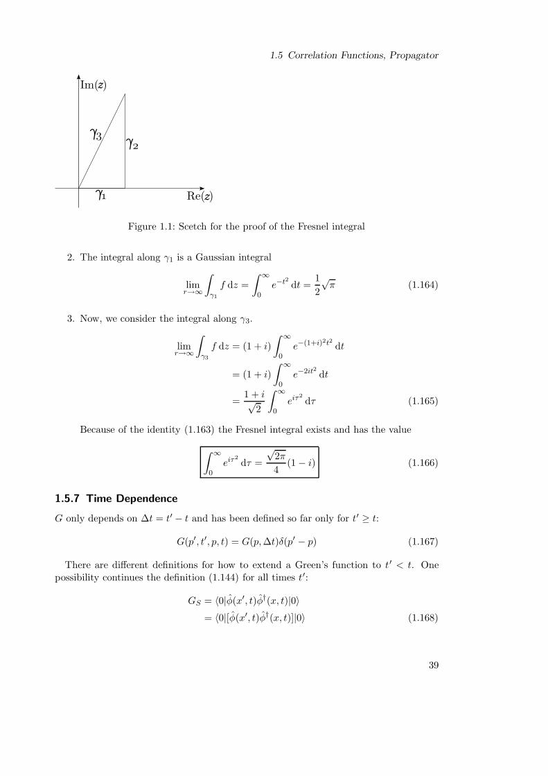
1.5 Correlation Functions, Propagator
Figure 1.1: Scetch for the proof of the Fresnel integral
2. The integral along γ1 is a Gaussian integral
limr→∞
∫
γ1
f dz =
∫ ∞
0e−t
2dt =
1
2
√π (1.164)
3. Now, we consider the integral along γ3.
limr→∞
∫
γ3
f dz = (1 + i)
∫ ∞
0e−(1+i)2t2 dt
= (1 + i)
∫ ∞
0e−2it2 dt
=1 + i√
2
∫ ∞
0eiτ
2dτ (1.165)
Because of the identity (1.163) the Fresnel integral exists and has the value
∫ ∞
0eiτ
2dτ =
√2π
4(1 − i) (1.166)
1.5.7 Time Dependence
G only depends on ∆t = t′ − t and has been defined so far only for t′ ≥ t:
G(p′, t′, p, t) = G(p,∆t)δ(p′ − p) (1.167)
There are different definitions for how to extend a Green’s function to t′ < t. Onepossibility continues the definition (1.144) for all times t′:
GS = 〈0|φ(x′, t)φ†(x, t)|0〉= 〈0|[φ(x′, t)φ†(x, t)]|0〉 (1.168)
39
1 Quantum Fields
We make a Fourier transform from time into frequency space.
GS(p, ω) =
∫ ∞
−∞eiω∆tGS(p,∆t) d∆t
=
∫ ∞
−∞ei∆t(ω−
p2
2M) d∆t
= 2πδ
(ω − p2
2M
)(1.169)
The spectral function
GS(p, ω) = 2πδ
(ω − p2
2M
)(1.170)
gives information about the particle content. Delta functions generally denote stableparticles. Unstable particles are characterized by resonance peaks with their decaywidth.
1.5.8 Higher Correlation Functions
We consider the scattering of two incoming particles with momentum p1 and p2 into twooutgoing particles with momentum p3 and p4. The transition amplitude for this event is
〈0|φ(p3, t′)φ(p4, t
′)φ†(p1, t)φ†(p2, t)|0〉. (1.171)
Here the incoming particles states refer to t→ −∞ (i.e. an incoming two particle statepresent long times before the scattering event) and outgoing ones to t′ → ∞.
We get a four-point function because we have two particles.We introduce the index notation
φα(p, t), α = 1, 2
φ1(p, t) = φ(p, t), φ2(p, t) = φ†(p, t) (1.172)
We furthermore consider n times with tn ≥ tn−1 ≥ · · · ≥ t1 and define
G(n)αn...α1
(pn, tn; pn−1, tn−1; . . . ; p2, t2; p1, t1)
= 〈0|φαn (pn, tn) . . . φα2(p2, t2)φα1(p1, t1)|0〉 (1.173)
1.5.9 Time Ordered Correlation Functions
We introduce the time ordering operator, it puts the later t to the left:
TO(t1)O(t2) =
O(t1)O(t2) if t1 > t2
O(t2)O(t1) if t1 < t2(1.174)
This operator is only well defined if t1 6= t2 or for t1 = t2 only if [O(t1), O(t2)] = 0.
40
1.5 Correlation Functions, Propagator
With the use of the time ordering operator we get
G(n)α1 ...α2
(pn, tn; pn−1, tn−1; . . . ; p2, t2; p1, t1)
= 〈0|Tφαn (pn, tn) . . . φα1(p1, t1)|0〉 (1.175)
which defines the Green’s function for arbitrary ordering of times. The time orderingoperator erases the information of the initial time ordering of the operators which pro-vides for much easier calculations. The Green’s function is now symmetric under theexchange of indices
(αj , pj , tj) ↔ (αk, pk, tk). (1.176)
This symmetry reflects the bosonic character of the scattered particles. For fermionsit will be replaced by antisymmetry.
Gn is the key to QFT. (1.177)
In future we will only compute time ordered Green’s functions.
1.5.10 Time Ordered Two-Point Function
As an example for the time ordered correlation functions we write down the time orderedtwo-point function using this formalism.
G(x′, t′, x, t) = 〈0|Tφ(x′, t′)φ†(x, t)|0〉
=
GS for t′ > t
0 for t′ < t
= GS(x′, t′, x, t)Θ(t′ − t) (1.178)
Notice that the limit t′ → t is simple for the spectral function but not a simple limit forthe time ordered correlation function since it is ill defined.
For the time ordered operator products we have the identities
T[A(t′), B(t)] = 0,
TA(t′)B(t) =1
2TA(t′)B(t) +
1
2TB(t)A(t′)
= T1
2A(t′), B(t)+. (1.179)
41

1 Quantum Fields
42

2 Path Integrals
2.1 Path Integral for a Particle in a Potential
At this point we take one step back and only consider a one-dimensional one-particleproblem in classical quantum mechanics without explicit time dependency. We can latereasily generalize it to 3D bosonic systems.
2.1.1 Basis of Eigenstates
In the Heisenberg picture we have the operators Q(t) and P (t) with the commutatorrelation
[Q(t), P (t)] = i (2.1)
and the Hamiltonian
H =P 2
2M+ V (Q). (2.2)
We introduce a basis of eigenstates |q, t〉 with
Q(t)|q, t〉 = q(t)|q, t〉. (2.3)
Note that the basis |q, t〉is only a basis of eigenstates of Q(t) at time t, it is not aneigenstate of Q(t′) for t′ 6= t. Don’t confuse this with the Schrodinger picture, wherethe states are time dependent. Here we work in the Heisenberg picture where |q, t〉 and|q, t′〉 are two different basis sets of time - independent states, one eigenstates of Q(t),the other of Q(t′). The states |q, t〉 are normalized at equal time to
〈q′, t|q, t〉 = δ(q′ − q). (2.4)
and the basis is complete
∫dq |q, t〉〈q, t| = 1 (2.5)
We also introduce a basis of eigenstates in momentum space |p, t〉with
P (t)|p, t〉 = p(t)|p, t〉. (2.6)
43
2 Path Integrals
Again |p, t〉is only a basis of eigenstates at time t, it is not an eigenstate of P (t ′) fort′ 6= t. The relations
〈p′, t|p, t〉 = 2πδ(p′ − p) and
∫dp
2π|p, t〉〈p, t| = 1 (2.7)
are similar to those for the position space.The transition from the basis in position space to the basis in momentum space is
defined through the relations
〈p, t|q, t〉 = e−ipq,
〈q, t|p, t〉 = eipq (2.8)
To avoid confusion we straighten out the connection of these states to the Schrodingerpicture. The state |q〉 of the Schrodinger picture is equivalent to the state |q, t = 0〉. Toget the state |q, t〉we need to time evolve the state |q〉 of the Schrodinger picture to get|q, t〉 = eiHt|q〉. Summarizing this we have
|q〉 = |q, t = 0〉 p = |p, t = 0〉|q, t〉 = eiHt|q〉 |p, t〉 = eiHt|p〉. (2.9)
Let’s check the relations mentioned above. We calculate the eigenvalue of Q(t)for aket |q, t〉by transforming into the Schrodinger picture and back again. The calculation
Q(t)|q, t〉 = Q(t)eiHt|q〉= eiHtQSe
−iHteiHt|q〉= eiHtQS |q〉= eiHtq|q〉= q|q, t〉 (2.10)
leads to the desired result. It is also immediately obvious that
〈p, t, |q, t〉 = 〈p|q〉 = e−ipq (2.11)
2.1.2 Transition Amplitude
The probability amplitude for a transition from an eigenstate of Q(t) to an eigenstateof Q(t′) is given by the transition amplitude:
G(q′, t′, q, t) = 〈q′, t′|q, t〉= 〈q′, t|e−iH(t′−t)|q, t〉 (2.12)
(We use here the symbol G since we will later see the analogy to the correlation functionwhen Q(t) is replaced by φ(x, t).) Our aim is now to give G(q′, t′, q, t) a path integralexpression. In order to do this, we will compute the transition amplitude for an infinites-imal time step dt, which is actually the only one that can be computed explicitly. In theend, we will make the limit procedure dt→ 0.
44

2.1 Path Integral for a Particle in a Potential
2.1.3 Infinitesimal Transition Amplitude
We are now interested in the infinitesimal transition amplitude
〈q′, t+ dt|q, t〉 = 〈q′, t|e−iH·dt|q, t〉. (2.13)
If we use the Taylor expansion of the exponential function, we get
〈q′, t+ dt|q, t〉 = 〈q′, t|1 − iHdt|q, t〉. (2.14)
Although the Taylor expansion of the exponential function up to first order is veryoften used in theoretical physics without worry to much about this, one usually has toshow, that terms of higher order are really unimportant in the limit dt → 0. This ismathematically very complicated and so we will not deal with this problem here.
We insert now the completeness relation 1 =∫ dp
2π |p, t〉〈p, t| into (2.14). We get
〈q′, t+ dt|q, t〉 =
∫dp
2π〈q′, t|1 − iHdt|p, t〉〈p, t|q, t〉 (2.15)
We now want to restrict ourselves to Hamiltonians of the form
H =
(P 2(t)
)2
2M+ V (Q(t)). (2.16)
The time dependence of the operators P and Q tells us that we will work in the Heisen-berg picture.
Actually, Hamiltonians that are given by (2.16) have a big advantage, because we cannow easily compute the matrix element of H appearing in equation (2.15):
〈q′, t|H|p, t〉 = 〈q′, t|(P (t))2
2M|p, t〉 + 〈q′, t|V (Q(t))|p, t〉 (2.17)
This is now very simple, because we can use the eigenstate properties of(P (t)
)2to the
ket vector and the eigenstate properties of V (Q(t)) to the bra vector. The result is
〈q′, t|H|p, t〉 =
(p2
2M+ V (q′)
)〈q′, t|p, t〉
= H(q′, p)〈q′, t|p, t〉, (2.18)
where q′ and p are now the position space and momentum eigenvalues to the operatorsQ(t) and P (t). Inserting this into equation (2.15) we get
〈q′, t|q, t+ dt〉 =
∫dp
2π
(1 − iH(q′, p)dt
)〈q′, t|p, t〉〈p, t|q, t〉. (2.19)
For the term (1 − iH(q′, p)dt) we can now write again the exponential function. Fur-thermore, the scalar products as well give exponential functions, so our infinitesimaltransition amplitude can be written as
〈q′, t+ dt|q, t〉 =
∫dp
2πexp (ip(q′ − q) − iH(q′, p)dt) (2.20)
45

2 Path Integrals
Please remember that this result is only valid for Hamiltonians that can be written as
H =
(P (t))2
2M +V(Q(t)
)and for really infinitesimal time steps, where terms proportional
to dt2 can be neglected. Imagine the difficulties we would be faced with, if we have anH2: in this case we could not compute the matrix element just by using the eigenstateproperties. It would be necessary to commute P and Q terms first.
Nevertheless, we are of course interested in transition amplitudes for finite time steps.Getting this out of our result for infinitesimal time steps will be the task of the nextparagraph.
2.1.4 Split of Amplitudes in Product of Infinitesimal Amplitudes
a) Split Time Interval
The basic idea is to split up a finite time interval t′ − t (t′ > t) into N + 1 infinitesimaltime steps. Therefore we insert N “lattice points” τi, i = 1 . . . N in time, so that we get
t < τ1 < τ2 < . . . < τN−1 < τN < t′. (2.21)
The time distance from each τi to the neighboring points is dτ . In the end we will dothe limit procedure N → ∞ what corresponds to dτ → 0.
b) Insert Completeness Relation
The transition amplitude we want to compute is
〈q′, t′|q, t〉. (2.22)
For every time point τi within the interval [t, t′], we have the completeness relation
∫dqi|qi, τi〉〈qi, τi| = 1. (2.23)
Inserting this completeness relation for every τi gives us
〈q′, t′|q, t〉 =
∫dq1dq2 . . . dqN 〈q′, t′|qN , τN 〉〈qN , τN |qN−1, τN−1〉〈q2, τ2|q1, τ1〉〈q1, τ1|q, τ〉
(2.24)
Remark that we have inserted 1 operators as an integration over position space variablesqi, not as an integration over momentum space variables pi like we did in paragraph 2.1.3,so there is no 2π missing here.
Our interim result is, that we can write our transition amplitude as a product of N+1infinitesimal time evolution steps, with integration over the N intermediate q(τi).
46

2.1 Path Integral for a Particle in a Potential
c) Infinitesimal Amplitudes
We have now reached the point, where we can use the result of the last paragraph. Everyinfinitesimal transition amplitude is given by
〈qj+1, τj+1|qj , τj〉 =
∫dpj+1
2πexp (i[pj+1(qj+1 − qj)] − iH(qj+1, pj+1)dτ) (2.25)
We will put this expression now into equation (2.24). Notice that this gives us now N+1integrations over pj , but that we still only have N integrations over qj . Furthermore,we remind ourselves that we could rewrite the appearing product of N + 1 exponentialfunctions (one for every infinitesimal amplitude) as an exponential function of N + 1summands. So we have now
〈q′, t′|q, t〉 =
∫ N∏
i=1
dqi
∫ N+1∏
j=1
dpj2π
exp
(i
[N+1∑
k=1
pk(qk − qk−1) −H(qk, pk)dτ
]), (2.26)
where q0 ≡ q and qN+1 ≡ q′. The 2π factor belongs to the product, so it appears N + 1times in this equation.
d) Notation
In order to write equation (2.26) a little bit more elegantly, we define
qk =qk − qk−1
dτ,
q(τ) =q(τ) − q(τ − dτ)
dτ. (2.27)
Here we used the additional definition τ ≡ t+kdτ (what implies t+(k−1)dτ ≡ τ −dτ).This looks reasonable, as qk is a position variable at time t+ kdτ and qk−1 is a positionvariable at time t + (k − 1)dτ . So in the limit dτ → 0 that we will perform later,our defined qk should have the meaning of a velocity (what we already imply here bychoosing the notation q ).
Anyway, for the moment we will just use equation (2.27) to simplify equation (2.26).We get
〈q′, t′|q, t〉 =
∫ N∏
i=1
dqi
∫ N+1∏
j=1
dpj2π
exp
(idτ
N+1∑
k=1
pkqk −H(qk, pk)
)(2.28)
2.1.5 Path Integral
With equation (2.28) we are just one step away from the path integral. We define it bythe limit procedure
∫Dq ≡ lim
N→∞
∫ N∏
i=1
dqi (2.29)
47

2 Path Integrals
and
∫Dp ≡ lim
N→∞
∫ N+1∏
j=1
dpj. (2.30)
Let us now discuss these equations a little bit:
• The integration∫Dq means, that for every intermediate time point τi our particle
may be everywhere, because we are integrating over all possible values of qi. Onlythe endpoints are fixed: q(t) = q, q(t′) = q′. To come from one endpoint toanother, all paths are allowed.
• Every path can be written as a function q(t). We are integrating over all thesefunctions. That’s why we will sometimes call our integrals “functional integrals”.
• Our paths don’t need to be very smooth. For all intermediate points, every valueis allowed, so we could have arbitrary strong oscillations.
• The integration∫Dp is, for the moment, without a further interpretation. It came
into our calculation just as integration variable. Nevertheless, we can already guessthat it will have something to do with the canonical momentum.
• For all calculations, we can only work with a large, but finite number of variables.Even if we use a computer, all data will be discrete and finite (and should be,unless we don’t want to wait for the results infinitely long).
• Anyway, the use of finite dτ should not play a role, if dτ is sufficiently small - wecannot resolve time arbitrary accurately by observations, e.g. nobody has observedthe Planck time tp = 10−42s yet.
• Furthermore, in the limit dτ → 0 nothing interesting should happen, as all physicalobservables should better have smooth limits. If a computation of a physicalobservable shows no smooth limit, it is most likely wrong, because otherwise itcould be used to resolve arbitrary small dτ .
2.1.6 Action
Let us now perform the p integration appearing in the expression for the transitionamplitude (2.28) in the case that
H =P 2
2M+ V (Q) (2.31)
Well, actually it is already implied that H can be written in this form, because thiswas an assumption we made to get our infinitesimal amplitude, that we used to come to(2.28).
48

2.1 Path Integral for a Particle in a Potential
First we rewrite the transition amplitude as
〈q′, t′|q, t〉 =
∫DqA exp
(−idτ
N+1∑
k=1
V (qk)
)(2.32)
with
A =
∫ N+1∏
j=1
dpj2π
exp
(−idτ
N+1∑
k=1
(p2k
2M− pkqk)
)=
N+1∏
j=1
Aj. (2.33)
Here Aj is defined as
Aj =
∫ ∞
−∞
dp
2πexp
(−idτ
[p2
2M− pqj
])(2.34)
Here it is no longer necessary to write p with an index. It is just an integration variable.Nevertheless, qj must still be written with index, because every Aj depends on onespecial qj.
The exponent in equation (2.34) looks almost Gaussian. In order to get a binomialformula, we make the ansatz
p2
2M− pqj =
1
2M(p− αqj)
2 − 1
2Mα2q2j =
p2
2M− α
Mpqj. (2.35)
So we must set α = M . With the variable substitution p′ = p −Mqj equation (2.34)becomes
Aj = exp
(−idτ
[M
2q2j
])·∫dp′
2πexp
(−idτ p
′2
2M
)(2.36)
Well, whatever the integration over p′ will give, it will just be a constant. We name thisconstant c and write
Aj = c exp
(−idτ
[M
2q2j
])(2.37)
Now it is quite easy to calculate A:
A = N exp(idτ
N+1∑
k=1
M
2q2k) (2.38)
with N = cN . Now we insert this in equation (2.32) and get
〈q′, t′|q, t〉 =
∫DqN exp
(idτ
[N+1∑
k=1
−V (qk) +M
2q2k
])
=
∫Dq exp
(idτ
[N+1∑
k=1
−V (qk) +M
2q2k + const
])(2.39)
49

2 Path Integrals
Let us define the following quantity:
S = dτ
(N+1∑
k=1
M
2q2k − V (qk) + const
). (2.40)
Now we can write
〈q′, t′|q, t〉 =
∫Dq eiS (2.41)
Obviously, in the limit dτ → 0, and if we neglect the irrelevant constant, the quantityS is exactly the action of a particle in a potential, just as we know it from classicalmechanics! There we have defined the action as
S =
∫ t′
tdτL(τ), (2.42)
with the Lagrangian
L =M
2q2 − V (q), q ≡ q(τ). (2.43)
We call the action S a functional of q(t) and write
S = S[q(t)] = S[q] = S[qk]. (2.44)
For a finite number of intermediate steps it depends on the N variables qk and on theboundary conditions q0 ≡ q and qN+1 ≡ q′ (that’s were the dependence of q and q ′ ofour matrix element 〈q′, t′|q, t〉 lies).
2.1.7 Interpretation of QM, Double Slit Experiment
The so called path integral formulation of QM is a method to calculate the probabilityfor a particle, which is at time t at the point q, to be at the point q ′ at time t′ > t.
The rule to compute that probability is as follows: Consider every path to get from qto q′. For every path k = 1, 2, . . . calculate a so called probability amplitude or simplyamplitude ψk, which is a phase factor ψk = eiSk . Calculate the total amplitude as thesum of the amplitudes of all paths, ψ =
∑k ψk. The probability for the particle to
propagate from |q; t〉 to |q′, t′〉 is then given by the square of the length of the complexnumber ψ.
This method is a generalization of the double slit experiment.Here we have
ψ = ψ1 + ψ2,
ψ1 = ψ1(q′) = 〈q′, t′|q1, τ〉〈q1, τ |q, t〉,
ψ2 = ψ2(q′) = 〈q′, t′|q2, τ〉〈q2, τ |q, t〉. (2.45)
This experiment can now be generalized in two ways:
50
2.1 Path Integral for a Particle in a Potential
1. Use more screens.
2. Cut more holes in each screen.
E.g. consider the following experiment with two screens and five holes.
Letting both the number of screens and the number of holes per screen go to infinity,we get the path integral formulation of QM. What is important is that the amplitude orphase factor of each path is given by eiS .
Note that this is a radically new way to formulate QM. There is no Schrodingerequation and no operators. But of course the two formulations must be equivalent inthe sense that they make the same physical predictions. We will later show how the oldoperator formulation of QM can be reconstructed.
But first let’s consider the relation to Classical Mechanics. Since the classical La-grangian L and action S appear, Classical Mechanics should be included in some limit.
2.1.8 Classical Path
We do a saddle point approximation, i.e. we expand the action S around the classicalpath q0(t).
S(q) = S(q0) +1
2
δ2S
δq(t)2
∣∣∣∣q0(t)
(q − q0)2(t) + · · · . (2.46)
There is no linear term since by definition q0(t) is an extremum:
δS
δq
∣∣∣∣q0(t)
= 0. (2.47)
Remember that in classical mechanics one shows that this principle of stationary actionis equivalent to the way to compute the path of a particle in Lagrangian formalism:
d
dt
∂L∂q
− ∂L∂q
= 0,
Mq +∂V
∂q= 0. (2.48)
So the basic difference between Classical Mechanics and Quantum Mechanics is:
Do not only consider the classical path, but also all other paths. (And includea phase factor.)
Obviously, for classical physics to be a good approximation, all higher terms have to besmall in comparison to the quadratic one.
Comment: Definition of functional derivativesIf you are not sure how to work with functional derivatives, go back to qn instead ofq(t). Then S is a normal function of the qn instead of a functional of q(t). When you
51

2 Path Integrals
have only finitely many n, the functional derivative becomes the gradient, i.e. a vectorof partial derivatives, just many of them:
δS
δq(t)≡ ∂S
∂qn,
δS
δq(t)q(t) ≡ ∂S
∂qnqn,
δS ≡∑
n
∂S
∂qnδqn,
1
2
δ2S
δq(t)2
∣∣∣∣q0(t)
(q − q0)2(t) ≡
∑
n,k
1
2
∂2S
∂qn∂qk
∣∣∣∣q0,n
(qn − q0)(qk − q0). (2.49)
Then at the very end do the limit procedure from normal derivatives to the functionalderivative. Let’s not worry about that now.
The saddle point approximation is a key concept, the whole perturbation theory isbased on it. That’s why we want to motivate it some more:
(a) Let’s first assume there is only one wall between the points q and q ′. That leads usto the functional
I =
∫ ∞
−∞eif(x). (2.50)
Assume that f(x) is purely imaginary, i.e. f(x) = ig(x) with some function g(x)that has a minimum at x0 and goes to infinity for x→ ±∞. Then
I =
∫ ∞
−∞e−g(x) (2.51)
converges, and the integral is dominated by the region around x0.
But say g(x) → C, i.e. g(x) levels off on the right side. Then the integral will notconverge.
To summarize: Under simple conditions, i.e. if f(x) is purely imaginary and goes toinfinity for |x| → ∞ not too slowly, convergence will be ok.
(b) Now let’s consider the case of many degrees of freedom q(τ) and the Euclidean actionS = iSE There the saddle point approximation for
∫Dq eiS =
∫Dq e−SE (2.52)
will often not converge.But there is a trick: Use imaginary time, i.e. substitute τ → iτ . Then analyticallycontinue the result and go back to real time.
52

2.1 Path Integral for a Particle in a Potential
(c) In the case of the Minkowski action, which is a real quantity, the integrands
eiS = cosS + i sinS (2.53)
are oscillatory functions and convergence is a very subtle issue. Sometimes it doesconverge, sometimes it does not.
The upshot that you should take home is this: For almost all interaction theories thesaddle point approximation never converges. Also, the theory of convergence of theseintegrals is a very complicated field of mathematics. Nevertheless, let’s do saddle pointapproximations as a working method, although things might not be well defined.
2.1.9 Operators
We now show how to calculate expectation values of operators, not only transitionamplitudes,
A = 〈q′; t′|A|q; t〉. (2.54)
(a) A = A(τ) = f(Q(τ), P (τ)), t < τ < t′ where A is an arbitrary function of Q(τ) andP (τ) ordered such that all factors P (τ) are on the left of Q(τ).
We go back to the definition of functional integrals and insert the states:
A =
∫dq(τ)
∫dp(τ)
2π〈q′; t′|p(τ); τ〉〈p(τ); τ |A(τ)|q(τ); τ〉〈q(τ); τ |q; t〉
=
∫dq(τ)
∫dp(τ)
2πA(q(τ), p(τ))〈q′; t′|p(τ); τ〉e−ip(τ)q(τ)〈q(τ); τ |q; t〉
=
∫DqDp A(q(τ), p(τ))ei
R t′
tp(τ)q(τ)−H(p(τ),q(τ)) (2.55)
(b) We consider the special case where A(τ) only depends on Q(τ). There we can carryout the P integration and find
A =
∫Dq A(q(τ))eiS . (2.56)
Note that this case is not so restrictive as it may seem, because it includes derivativeoperators, e.g. Q(τ), since they are sums of operators:
Q(τ) =Q(τ + dτ) −Q(τ)
dτ. (2.57)
The expectation value depends linearly on operators, i.e. for sums we have
〈q′; t′|∑
k
Ak|q; t〉 =∑
k
〈q′; t′|Ak|q; t〉 =
∫Dq AkeiS . (2.58)
53

2 Path Integrals
(c) Time ordered products A = An(τn) . . . A2(τ2)A1(τ1) with t < τ1 < τ2 < · · · <τn < t′. For simplicity, let’s say that the operators only depend on Q: Ak =Ak(Q(τk)). This can later be generalized to include a P dependence as well: Ak =Ak(Q(τk), P (τk)). Then
A = 〈q′; t′|An . . . A1|q; t〉 =
∫Dq An(qn, τn) . . . A1(q1, τ1)e
iS . (2.59)
The path integral expression for A does not depend on the ordering of the factorsAn(qn, τn) . . . A1(q1, τ1). We have a path integral formula for arbitrary time-orderedn-point functions!
〈q′; t′|TAn(τn) . . . A1(τ1)|q; t〉 =
∫Dq An(τn) . . . A1(τ1)e
iS (2.60)
The time ordering is crucial! This works because time-ordered products are commu-tative. We have arrived at a formulation that involves no q-numbers (i.e. operators),only c-numbers (i.e. complex numbers).(Dirac invented these names to emphasize that one can most of the time calculatewith functions, operators and any other mathematical object as if they were num-bers, just that some of these things are commutative (then they are called c-numbers)and some are not (then they are called q-numbers).
2.1.10 Can One Construct QM from a Path Integral?
In the last section we have introduced the path integral formalism, starting from the usualquantum mechanical operator formalism. Now one may ask whether both formulationsare really equivalent, i. e. if one can also derive the quantum mechanical operatorsfrom a path integral. In fact it is possible, but we will only sketch the proof here. Theinterested reader may try to formulate it in more detail. The most important result wederived previously is that we can express an operator expectation value through a pathintegral:
〈q′, t′|TA1(τ1) . . . An(τn)|q, t〉 =
∫Dq A1(τ1) . . . An(τn)e
iS , t′ > t, (2.61)
where S =∫dτL(τ), L = L(q(τ), q(τ), . . .) is the action describing the problem. Note
that the right-hand side does not depend on the order of the operators, since A1, . . . ,An are only c-numbers, in contrast to A1, . . . , An on the right-hand side. Now be Aan arbitrary time-ordered operator, i. e. A = TA. Now as explained above, we havea prescription how to compute 〈q′, t′|A|q, t〉 in the case t′ > t. This means that we cancompute the matrix elements of A between two different bases, namely |q(t)〉 and |q(t′)〉.What we want of course is to express A in one given basis |q, t〉. So we have to make achange of basis by
〈q′, τ |A|q, τ〉 =
∫dq1
∫dq2〈q′, τ |q2, t′〉〈q2, t′|A|q1, t〉〈q1, t|q, τ〉, (2.62)
54
2.2 Functional Integral for Bosonic Many-Body Systems
where t < τ < t′. On the right-hand side of the equation, there are three expectationvalues which can essentially be determined by the path integral formalism (in the casewhere the time value on the left hand side is smaller than the one on the right-handside, we can use the formalism to compute the complex-conjugate). Then once we havedetermined an operator in a complete basis, we of course completely know the operator.Since the commutator of two operators is also an operator, they can be computed in thesame way and we will find for instance [Q(τ), Q(τ)] 6= 0. To find the momentum operatorP , we remember that it is defined classically by p(τ) = ∂L
∂q(τ) . In this way, we will get P
as a function of q(τ) and q(τ), which is often just P = MQ. Inserting this expressionin the path integral, we can determine the momentum operator in a complete basis.Additionally, one can derive the right canonical commutator relation [Q(τ), P (τ)] = i.The fact that we end up with non-vanishing commutators results from the fact that wego from integrals to matrix elements, and in general matrices do not commute.
2.1.11 Generalization to N Degrees of Freedom
To prepare the use of the path integral formalism in quantum field theory, we willgeneralize to N degrees of freedom. This is actually straight forward, we just add anindex and define quantities Qj(t), Pj(t) with canonical commutators [Qi(t), Pj(t)] = i.The integral will be generalized to
∫Dqj(t) and the action will of course depend on all
degrees of freedom, i. e. we have S[qj(t)].
Examples:
• One atom in 3D: j = 1, 2, 3, N = 3, and Qj(t) corresponds to a 3-vector Q(t).
• N atoms in d=1 lattice: j = 1, . . .N , Qj(t)
• continuum notation: N , Qj(t) → Q(x, t)
• fields: N → ∞
• lattice in 3D, only one excitation direction: Q(x, t)
• lattice in 3D, 3D excitations: Q(x, t)
Especially the fifth example is very important, since this will correspond to scalar fieldsin quantum field theory.
2.2 Functional Integral for Bosonic Many-Body Systems
2.2.1 Path Integral for QFT
Now of course we aim to use the derived functional integral formalism (i. e. the pathintegral formalism) in quantum field theory. There we have fields φ(x, t), φ†(x, t) and
55

2 Path Integrals
the canonical commutator relation [φ(x′, t), φ†(x, t)] = δ(x − x′). Then we can defineposition and momentum operators by
Q(x, t) =1√2(φ(x, t) + φ†(x, t)),
P (x, t) = − i√2(φ(x, t) − φ†(x, t))). (2.63)
As a simple exercise, the reader may show that
[Q(x′, t), P (x, t)] = iδ(x− x′). (2.64)
Now we will consider a simple system of non-interacting bosonic atoms with a Hamilto-nian
H =
∫
x
1
2M∇φ†(x, t)∇φ(x, t) + V (x)φ†(x, t)φ(x, t)
(2.65)
and derive the functional integral for this system. We use the inverse transformation of(2.63),(2.63) given by
φ =1√2(Q+ iP ),
φ† =1√2(Q− iP ) (2.66)
where we have suppressed the arguments x and t. In the same way we can compute
φ†φ =1
2(Q− iP )(Q+ iP ) =
1
2(Q2 + P 2) + i[P,Q] =
1
2(Q2 + P 2) + const., (2.67)
where we have introduced an infinite constant. However, this constant will drop out ofthe Hamiltonian anyway, since we are free to choose any zero-point of energy we considerappropriate. Now we can write the Hamiltonian as
H =
∫
x
1
2Q(x, t)(− ∆
2M+ V (x))Q(x, t) +
1
2P (x, t)(− ∆
2M+ V (x))P (x, t). (2.68)
Now let’s have a look at transition amplitudes and the expectation values of operators:We introduce the notation |q(x, t)〉 = |q(x, t), t〉 = |q, t〉. The position operator Q will acton this basis as Q(x, t)|q(x, t)〉 = q(x, t)|q(x, t)〉. The expectation value of a time-orderedproduct of operators can be expressed as usual by
〈q′(x′, t′)|TA1(x1, t1), . . . , An(xn, tn)
|q(x, t)〉 =
∫Dq
∫DpA1(x1, t1) . . . An(xn, tn)e
iS ,
(2.69)where the action S is defined as S =
∫dτdxL(x, τ) with the Lagrangian L(x, τ) =
p(x, τ)q(x, t) − H(p(x, τ), q(x, τ)). Further∫Dq =
∫Dq(x, t). In the case of finite
degrees of freedom, this corresponds to integration over every degree of freedom. In thecontinuum case, we therefore integrate over infinitely many degrees of freedom. Now of
56

2.2 Functional Integral for Bosonic Many-Body Systems
course, we want to express the action in terms of the fields φ and φ†. We rememberthe expressions (2.66),(2.66) and define
∫DqDp =
∫DφDφ∗ =
∫Dφ. This can be
understood by remembering that a complex field φ has two degrees of freedom, forexample the real and the imaginary part. In the same way, one can also treat φ and φ∗
independently. Now we are actually no longer integrating over paths, but we integrateover all possible configurations in space and time, each having a certain phase factor.This is in fact very similar to statistical mechanics. In the 3D Ising model, we have acubic lattice with lattice sites i = (n1, n2, n3) with a certain spin si = ±1. The partitionfunction is given by Z =
∑siTre−βH , where we have to sum over all possible spin
configurations. This is very similar to what we have in quantum field theory. In fact ifwe assume that our bosonic atoms are located on a grid, we have only a finite numberof degrees on freedom in QFT and instead of the integral we will also have sums overall possible configurations in space. The other difference is that in statistical mechanics,the exponential factor is real, while it is imaginary in QFT. In fact we will later showthat we can make a transformation t 7→ it in QFT so that the exponential factor willalso become real.
Lagrangian Density in Terms of φ and φ†
Now we wish to express the Lagrangian density L in terms of φ and φ†. For this look atthe Hamiltonian H, expressed in terms of φ and φ†:
H =1
2q(x, t)
(− ∆
2M+ V (x)
)q(x, t) +
1
2p(x, t)
(− ∆
2M+ V (x)
)p(x, t)
=φ†(x, t)(− ∆
2M+ V (x)
)φ(x, t) (2.70)
L is calculated by
L = pq −H(p, q) (2.71)
with
pq = − i
2(φ− φ∗) ∂t (φ+ φ∗) = − i
4∂t(φ2 − φ∗2 + 2φφ∗
)+ iφ∗∂tφ (2.72)
When calculating the action S, the first term drops out, because it is a total timederivative. For S we therefore have
S =
∫dtdx
(iφ∗∂tφ− φ∗
(− ∆
2M+ V (x)
)φ
)(2.73)
This is the functional integral for bosonic atoms in a trap! Here we can see, indeedprovokes an exponential decay, depending on the time dependence of φ!
57

2 Path Integrals
2.2.2 Systems in Various Dimensions d
Up to now, we have been investigating systems in real space with dimension d=3. Thecases d=2, d=1 just relate to QFT on the surface, on the line respectively, by addingconstraints in d=3. The case d=0 is however somewhat special. Here the atoms areconfined to points, the so called quantum-dots. Let’s take a look at the action S ford=0:
S =
∫dt
(iφ∗(t)∂tφ(t) + µφ∗(t)φ(t) − λ
2(φ∗(t)φ(t))2
)(2.74)
and compare it with the action in QM:
SQM =
∫dt
(p(t)q(t) − p2(t)
2M− V (q(t))
)→∫dt
(1
2Mq2(t) − V (q(t))
). (2.75)
We see that although they are different actions, they have the same structure. So wecan say for d=0:
QFT := QM (2.76)
Another Comparison of QFT and QM
In QM there are, like you know only a finite number of degrees of freedom. q(t) describesa particle in a potential and φ(t) describes a quantum dot. By adding more dimensions
to φ(t), that means looking at φ(x, t), we enter QFT, and get infinite degrees of freedom.The same on the operator level:
Q↔ φ(x) (Schrodinger)
Q(t) ↔ φ(x, t) (Heisenberg) (2.77)
2.2.3 In and Out States
Now we would like to look at a scattering experiment. In short: 2 or more particles arrivethe interaction region, and several particles are scattered out. Before the scattering, wehave well separated incoming particles (they don’t influence each other!), and after thescattering also well separated outgoing particles.
We assume the interaction timescale tint = 0. In experiments the timescale texp isfinite, but since we look at times t < 0 with |t| texp, and assume the incomingparticles are well separated, we can also assume texp ≈ 0.At t → −∞, we have the incoming N -particle state, and at t → ∞, the outgoing N -particle state. The incoming state is characterized by the occupation number N , theexternal properties of the particles (such as the momenta p1, . . . , pN ) and the internalproperties (like the spins j1, . . . , jN , the flavors, etc.)
|N, p1, . . . , pN , j1, . . . , jN 〉 ≡ |α〉 (2.78)
58

2.2 Functional Integral for Bosonic Many-Body Systems
where α is a multi index! The outgoing state is characterized by |β〉. These states areeach a complete basis in Fock space. Now for the incoming state at some fixed t , wecan also take an eigenbasis to the occupation operators ni(p, t), for example φ†j(p, t)|0; t〉,or 1√
2φ†j1(p1, t)φ
†j2
(p2, t)|0; t〉, but remember: the basis depends on t in a sense, that t
indicates at which time the basis is an eigenbasis to the ni(p, t)!
We label the incoming vacuum state |0; t〉, t→ −∞ as |0; in〉, the outgoing state willbe labeled |0; out〉.
The basis |α, in〉 (|α, t〉, t → −∞) is a complete basis of in states, and the basis|β, out〉 is a complete basis of out states, but they are not identical. They can havean overlap, which means there is a transition amplitude. This leads us to the . . .
2.2.4 S-Matrix
The transition amplitude
Sβα = 〈β, out|α, in〉 (2.79)
is called the S-matrix. We have to study this basic concept because it is crucial fordescribing scattering experiments. It tells us how the system has evolved, with the exis-tence (or nonexistence) of an interaction. If the system has no potential and interaction,we expect that |α, in〉 and |β, out〉 are orthogonal. But what if there is an interaction?This interaction would certainly change the properties of the particles, and thus the state|α, in〉. But there are of course conservation laws, like energy and momentum conserva-tion, which as we will see be already implemented in Sβα. In fact all the information ofthe physics in the interaction is contained in the S-matrix, wonderful, right? So let usexplore Sβα.
First of all the completeness of |α, in〉 and |β, out〉 leads to the fact that S is unitary.Let’s see why.First we show S†S = 1:
S†S =∑
β
(S†)γβSβα =
∑
β
〈β, out|γ, in〉∗〈β, out|α, in〉
=∑
β
〈γ, in|β, out〉〈β, out|α, in〉
=〈γ, in|α, in〉 = δγ,α (2.80)
In (2.80) we used the completeness of |β, out〉.
2.2.5 Functional Integral for the S-Matrix
By now, we know the functional integral for time ordered operators
〈q(x′, t′)|TA1(t1) . . . An(tn)|q(x, t)〉 =
∫DφA1(t1) . . . An(tn)e
iS (2.81)
59

2 Path Integrals
with Ak(tk) = Akφ(tk), φ†(tk),
˙φ(tk) . . .. But this is not yet the S-matrix. Now because
we have Q(x, t)|q(x, t)〉 = q(x, t)|q(x, t)〉 and Q(x, t) = 1√2
(φ(x, t) + φ†(x, t)
), we can
write the time ordered products as functions ofQ(x, t), and thus the integrals as functionsof q(x, t). To set up a functional integral for S, we just insert ones in the limits ±∞:
Sβα = 〈β, out|α, in〉
= limt→∞,t′→−∞
∫dq(x, t)dq(x′, t′)〈β, out|q(x′, t′)〉〈q(x′, t′)|q(x, t)〉〈q(x, t)|α, in〉
= limt→∞,t′→−∞
∫dq(x, t)dq(x′, t′)〈β, out|q(x′, t′)〉
(∫D′φeiS
)〈q(x, t)|α, in〉
(2.82)
Now in (2.82) we have the path integral∫D′ that still has the boundary conditions at
q and q′. But now we integrate over these boundaries, and thus yield an unconstrainedpath integral:
Sβα = limt→∞,t′→−∞
∫Dφ〈β, out|q(x′, t′)〉〈q(x, t)|α, in〉 (2.83)
We would now like to investigate a 2 → 2 scattering. The in and out states are givenby
|α, in〉 = φ†(p1, t)φ†(p2, t)|0, in〉
〈β, out| = 〈0, out|φ(p3, t′)φ(p4, t
′). (2.84)
The S-matrix is then a 4-point correlation function:
Sβα = 〈β, out|α, in〉 =〈0, out|φ(p3, t′)φ(p4, t
′)φ†(p1, t)φ†(p2, t)|0, in〉
=〈0, out|T(φ(p4, t
′) . . . φ†(p1, t))|0, in〉. (2.85)
For time ordered operators A we want to find the matrix elements for the vacuum inand out states:
〈0, out|T(A[φ(x, t), φ†(x, t)
])|0, in〉
= limt→−∞,t′→∞
∫dq(x, t)dq(x′, t′)〈0, out|q(x′, t′)〉〈q(x′, t′)|T
(A)|q(x, t)〉〈q(x, t)|0, in〉
=
∫Dφ(x, t)A (φ(x, t), φ∗(x, t)) eiS−η (2.86)
where e−η = f∗(q(x′, t′))f(q(x, t)) = 〈0, out|q(x′, t′)〉〈q(x, t)|0, in〉 can be neglected. Sowe have, now in momentum space
〈0, out|T(A[φ(p, t), φ†(p, t)
])|0, in〉 =
1
Z
∫Dφ(p, t)A (φ(p, t), φ∗(p, t)) eiS[φ]. (2.87)
60
2.2 Functional Integral for Bosonic Many-Body Systems
Normalization
We calculate the matrix element of unity, and define it to be 1:
〈0, out|0, in〉 =1
Z
∫DφeiS = 1
⇒ Z =
∫DφeiS . (2.88)
This actually means that the in and out states are the same! To see this remember that|0, t〉 = eiE0t|0〉!
So all in all the S-matrix of a time ordered operator A is
〈0, out|T(A)|0, in〉 =
∫DφAeiS∫DφeiS . (2.89)
Summarizing our previous considerations, we can give an exact expression for the vacuum-expectation value of any time-ordered operator TA by
〈0|TA|0〉 =
∫DφAeiS∫DφeiS
. (2.90)
In the same way we can compute the S-matrix for 2-2 scattering by
Sβα = Z−1
∫Dφφ(p4, t
′)φ(p3, t′)φ∗(p2, t)φ
∗(p1, t)eiS , (2.91)
where we used the abbreviation Z =∫DφeiS and where we consider t → −∞ and
t′ → +∞.
2.2.6 Correlation Function
Now in the same way, we can express time ordered correlation functions in vacuum by
〈0|Tφα1 (t1) . . . φαn(tn)|0〉 = Z−1
∫Dφφα1 . . . φαn(tn)e
iS[φ] =: 〈φα1(t1) . . . φαn(tn)〉,(2.92)
where we introduced the last expression as a simple convention. The index α used hereis a multi index and includes:
• position or momentum variables as the argument for the operator
• internal indices
• whether we refer to φ or φ†. In fact this can be interpreted as an additional internalindex in the basis of real fields, having φ = 1√
2(φR + iφI).
So for a given action, the correlation functions can be computed. However one may aska couple of questions, i. e.:
61

2 Path Integrals
• How do we recover the concept of particles?
• What fields should be chosen? In an integral one can make variable transformationsφ→ φ′[φ]! For example, what is the normalization of φ? These questions may seemtrivial in the examples we have considered so far, but they are very important inmore complicated situations where the particles are not known from the beginning,like the pions in QCD!
• How is time-ordering realized in practice?
〈φ(p′, t′)φ∗(p, t)〉 6= 0 t′ > t= 0 t′ < t
Now let’s turn to the mathematical regularization of S: For this purpose we add a termiε∫dtd3xφ∗(x)φ(x). Then the phase factor in the functional integral transforms as
eiS → eiSe−εR
φ∗φ. The limit ε → 0+ will be done at the very end of the calculation,so that we always have well-defined integrals in the intermediate steps. This procedurecan be seen in various ways: First of all, if the functional integral is well-defined, thislimit should exist. On the other hand, if it is not, then we can just define the functionalintegral by this limit procedure. From the physical point of view, the reader may evenremember that we had a similar term when we first derived the path integral for theS-matrix, this term was just very small and therefore neglected.
2.2.7 Two-Point Function in Free Theory
We consider a simple example, where the action in the momentum basis is given by
S0 =
∫dt
d3p
(2π)3iφ∗(p, t)∂tφ(p, t) −E(p)φ∗(p, t)φ(p, t) (2.93)
with E(p) = p2
2M . We can even simply this expression going to frequency space by
φ(p, t) =
∫dω
2πe−iωtφ(ω, p). (2.94)
Now we can write the action in frequency-momentum space, where it becomes diagonal(in time-momentum space, it involves a time derivative, which implies that values atdifferent times are compared, though they are infinitely small in the continuum limit).
S =
∫dω
2π
d3p
(2π)3(ω −E(p))φ∗(ω, p)φ(ω, p) (2.95)
The functional integration in frequency-momentum space is defined by
∫Dφ =
∏
ω,p
∫ +∞
−∞dφ(ω,p)dφ∗(ω,p). (2.96)
62

2.2 Functional Integral for Bosonic Many-Body Systems
This can be understood by going back to discrete time and space with torus boundaryconditions at large t and −t and a finite volume of space with periodic boundary con-ditions. In such a configuration, frequency-momentum space will also consist of a finitelattice of points (ω,p). Now we define the free propagator by
G0(p′, p) = 〈φ(p′)φ∗(p)〉0 = Z−1
∫Dφφ(p′)φ∗(p)eiS0 , (2.97)
using p = (ω,p). To compute the free propagator, we first need some Gaussian integrals:
∫ +∞
−∞dxe−αx
2=
√π
α,
∫dφdφ∗e−αφ
∗φ =π
α,
∫dφdφ∗φ∗φe−αφ
∗φ = − ∂
∂α
∫dφdφ∗e−αφ
∗φ =π
α2,
∫dφdφ∗φ∗φe−αφ
∗φ
∫dφdφ∗e−αφ∗φ
=1
α,
∫dφdφ∗φe−αφ
∗φ =
∫dφdφ∗φ∗e−αφ
∗φ = 0. (2.98)
Now computing G0, there are only contributions for (ω,p) = (ω ′,p′). Then we can usethe above calculated Gaussian integrals by putting α = −i(ω−E(p)), yielding the veryimportant result
G0(p′, p) = 〈φ(p′)φ∗(p)〉 =
i
ω −E(p)δ(p′ − p), (2.99)
where δ(p′ − p) = (2π)4δ(ω′ − ω)δ3(p′ − p).
Time-Dependent Two-Point Function
Now we compute the time-dependent two-point function. For this purpose, we have togo from frequency space to time dependent functions. Then we can use the previousresult and get
〈φ(p′, t′)φ∗(p, t)〉 =
∫dω
2π
dω′
2πe−iω
′t′eiωt〈φ(ω′, p′)φ∗(ω, p)〉
= (2π)3δ3(p− p′)∫
dω
(2π)e−iω(t′−t) i
ω −E(p)
= (2π)3δ3(p− p′)e−iE(p)(t′−t)A,
A =
∫dω
2πe−iω(t′−t) i
ω, (2.100)
where we defined ω = ω − E(p). As we can see, A has a pole on the real axis. Toregularize the integral, we introduce a shift ω → ω + iε with some positive ε. As wediscussed previously, for a well-defined functional integral there should be a smooth limitε → 0+. Otherwise, we just define the functional integral by this limit. The shift in ω
yields ω → ω + iε and therefore eiS ∝ eiωφ∗φ→eiωφ
∗φ−εφ∗φ. The pole in the expression
63

2 Path Integrals
for A is now below the real axis in the space of complex ω. To evaluate the integral,we close the contour integral below the real axis for t′ > t, and above the real axis fort′ < t, yielding
A =
1 t′ > t0 t′ < t
= θ(t′ − t) (2.101)
according to the residue theorem. This already answers one of the questions we wereasking above, i. e. how time ordering arises in practise. It is realized by the appropriatechoice where to close the contour lines. As a result we get the useful formula
∫ +∞
−∞
dω
2π
i
ω −E(p) + iεe−iω(t′−t) = e−iE(p)(t′−t)θ(t′ − t). (2.102)
So we get the following result for the free propagator in time-momentum space, inagreement with our previous calculations:
〈φ(p′, t′)φ∗(p, t)〉 = (2π)3δ3(p − p′)e−iE(p)(t′−t)θ(t′ − t) = 〈0|Tφ(p′, t′)φ†(p, t)|0〉.(2.103)
2.2.8 S-Matrix Element in One-Particle Channel
Now we can compute the S-matrix in the one-particle channel, i. e. for one ingoing andone outgoing particle. It is given by
Sp′p = δ(p′ − p)e−iE(p)(t′−t). (2.104)
We want to make some comments on this result:
1. The phase factor in the S-matrix element is irrelevant, we will see that only |S|2matters at the end.
2. The phase can be eliminated by multiplying Sβα with standard phase factors:
• e−iEi(pi)t for every incoming particle,
• eiEi(pi)t′for every outgoing particle.
3. This means that phase factors can be absorbed in a redefinition of the variablesφ(p). With this convention, Sβα is normalized in comparison with free theory. Thiscan be formally implemented in the general definition of Sβα. Then the statementSβα = δβα is true if and only if we have a free theory.
2.2.9 Reduced Transition Amplitude M
If we want to consider scattering of particles, we need to consider a deviation of S fromunity. Therefore we define
Sβα = δβα − i(2π)4δ(Ef −Ei)δ3(pf − pi)Mβα, (2.105)
64

2.2 Functional Integral for Bosonic Many-Body Systems
where the delta functions imply energy and momentum conservation. Let’s consider anexample of two incoming and several outgoing particles, then we have pi = p1 + p2
and pf is the total momentum of the outgoing particles. Then we can compute thedifferential cross section from M by
dσ =∏
f
d3pf(2π)3
1
|v1 − v2|(2π)4δ(Ef −Ei)δ
3(pf − pi)|M(p1, p2 → pf)|2, (2.106)
where v1 − v2 is the relative velocity of the incoming particles. More generally, Mcontains the dynamic information, but not the kinematics.
2.2.10 Classical Approximation for 2 → 2 Scattering
In the sections 2.2.7 and 2.2.8 we discussed the two-point function in free theory, thusthe one-particle channel. Now we want to go a step further and compute the four-pointfunction in the classical approximation, that is also called “Born Approximation” or“Tree Approximation” and simply means that we consider only pointlike interaction oftwo particles.
The action in time and position space is
S =
∫dτ
∫d3x
(iϕ∗(x, τ)∂τϕ(x, τ) − 1
2M∇ϕ∗(x, τ)∇ϕ(x, τ) − λ
2(ϕ∗(x, τ)ϕ(x, τ))2
)
(2.107)
and we want to know the S-matrix elements
Sβ,α = 〈β, out|α, in〉= 〈p4,p3, out||p1,p2, in〉= 〈0|ϕ(p4, t
′)ϕ(p3, t′)ϕ†(p2, t)ϕ
†(p1, t)|0〉 (2.108)
We know that this time ordered product of operators has the following path integralexpression:
Sβ,α = f
∫Dϕϕ(p4, t
′)ϕ(p3, t′)ϕ∗(p2, t)ϕ
∗(p1, t)eiS
∫DϕeiS . (2.109)
f is a factor that is given by
f = e−i(E(p1,t)+E(p2 ,t))e+i(E(p3,t′)+E(p4,t′)) (2.110)
and that will compensate some phases that come out of the calculation later. It is justthe same here as it was in section 2.2.8, where we defined our S-matrix element.
Well, equation (2.109) is the basic problem that we will solve in this section. We willdo this in two steps. First we will consider the free theory with λ = 0, and then we willturn on the interaction.
65
2 Path Integrals
a) Free theory for 2 → 2 “Scattering”
Actually, the title of this paragraph is a little bit confusing. Of course, in a free theorywith λ = 0 we expect no scattering at all.
The first thing that we have to do, is that we should use the representation of theaction S in momentum space instead of (2.107), because the field variables also dependon momenta:
S =
∫dt
∫d3p
(2π)3(iϕ∗(p, t)∂tϕ(p, t) −E(p)ϕ∗(p, t)ϕ(p, t)) (2.111)
The functional integrals in (2.109) are also to be understood as functional integrals overfield variables, that depend on momenta and time or frequency
∫Dϕ =
∫Dϕ(p, t) =
∫Dϕ(p, ω) (2.112)
Do you feel completely familiar with equation (2.109)? Do you know, what the dif-ferent arguments of the functions tell us and where they came from? If not, read thefollowing small insertion. If yes, proceed to the next paragraph that is called Fouriertransformation to frequency space .
• Small insertion to discuss the meaning of equation (2.109)
In section 2.1, we defined what a path integral is:
∫Dq =
∫ N∏
k=1
dqk (2.113)
So it is an integral over all intermediate steps. As every qk coordinate corresponds to acertain time, we could also write for example
∫Dq =
∫ N∏
k=1
dq(tk) (2.114)
or, if we like ∫Dq =
∫ ∏
t
dq(t). (2.115)
So no matter how we write it, we always mean the same: A product of integrals over allintermediate steps. Remark, that for different t’s, we simply mean different integrationvariables! This will be extremely important later on.
So far, we only considered quantum mechanical path integrals, or, if we want to say it inthe words of 2.2.2, a 0-dimensional Quantum Field Theory. If we go to infinitely manydegrees of freedom, our path integral function q depends not only on t, but now on x andt: ∫
Dq =
∫ ∏
x,t
dq(x, t) (2.116)
where we mean the integration over all intermediate steps in space and time. But if x is the“real” space coordinate, one may ask the question what is the meaning of q? To answer
66

2.2 Functional Integral for Bosonic Many-Body Systems
this question remember, that q(x, t) is the eigenfunction to the Operator Q(x, t)! Thecorresponding classical quantity was Q(x, t), which was in the solid-picture the distanceof the oscillator at space position x at time t to its equilibrium position. Of course, thisis not an explanation of what it is in the case of a “real” vacuum without an underlyingsubstructure of atoms like we have it in the solid. But anyway you should keep in mind,that in the QFT-path integral the real space coordinate is x, and not the integrationvariable q.
Again, you should remark, that for different (x, t) we mean different integration variablesq.
Of course we had a similar expression for momenta p:∫
Dp =
∫ ∏
x,t
dp(x, t). (2.117)
The next step is now to “exchange” our integration variables q(x, t) and p(x, t) into fieldvariables ϕ(x, t) and ϕ∗(x, t). Ignoring the arguments for a short while, this is accordingto
q =1√2(ϕ + ϕ∗),
p = i1√2(−ϕ+ ϕ∗) (2.118)
just a rotation with Jacobian 1. Thus, we have now∫
Dq(x, t)∫
Dp(x, t) =
∫Dϕ(x, t)
∫Dϕ∗(x, t). (2.119)
The vacuum expectation value of a time-ordered product of operators TA(ϕ(y, t), ϕ†(y, t))is given by the following path integral, where we write now once all dependencies:
〈0|TA(ϕ(y, t), ϕ†(y, t))|0〉 =
∫Dϕ(x, t)
∫Dϕ∗(x, t)A(ϕ(y, t′), ϕ∗(y, t′))eiS[ϕ(x,t),ϕ∗(x,t)]
∫Dϕ(x, t)
∫Dϕ∗(x, t)eiS[ϕ(x,t),ϕ∗(x,t)]
(2.120)
Please note that the difference between the x and y is important (and so is the difference
between t and t′)! The operator A consists of creators and annihilators, that create andannihilate particles at particular points in space y , while the x are arguments of theintegration variables! Anyway, equation (2.120) is not formal perfect. Please imagine thatany ϕ and ϕ∗ acts at different times and at different points in space, and of course not allat time t and at the same position y, and that we have to order the product of operatorswith respect to the different times ti when they act.
Well, we have now almost explained equation (2.109). What remains is the transition fromposition space to momentum space. Unfortunately we are once more confronted with alack of variable names. So we name our integration variable p, although it is not the samep that appeared a few lines above in equation (2.117). That p corresponded to q, whileour p that we have now corresponds to x.
Anyway, under the assumption that the transition∫
Dϕ(x, t)
∫Dϕ∗(x, t) →
∫Dϕ(p, t)
∫Dϕ∗(p, t) (2.121)
67

2 Path Integrals
has Jacobian 1, we finally get our equation (2.109), if we set A to be the operator thatcorresponds to the four-point function that we want to compute:
Sβ,α = f
∫Dϕ(p, t)
∫Dϕ∗(p, t)ϕ(p4, t4)ϕ(p3, t3)ϕ
∗(p2, t2)ϕ∗(p1, t1)e
iS[ϕ(p,t),ϕ∗(p,t)]
∫Dϕ(p, t)
∫Dϕ∗(p, t)eiS[ϕ(p,t),ϕ∗(p,t)]
.
(2.122)
In contrast to (2.109), we used ti so that we don’t mix up the integration variables t withthe special times t1 and t2 before and t3 and t4 after the scattering process.
Fortunately a possible double use of times will now have an end. Because here, our small
excursion ends and the next step is the. . .
Fourier transformation to frequency space
The Fourier transformation from time to frequency space is quite simple. As wealready used
ϕ(x, t) =
∫d3p
(2π)3eipxϕ(p, t) (2.123)
the transformation to frequency space is of course
ϕ(p, t) =
∫dω
2πe−iωtϕ(p, ω) (2.124)
so the overall transformation is
ϕ(x, t) =
∫d3pdω
(2π)4eipx−iωtϕ(p, ω). (2.125)
To shorten the notation, we will write this very often as
ϕ(x, t) =
∫d4p
(2π)4eipxϕ(p, ω), (2.126)
with four-vectors p = (ω,p) and (px) = −p0x0 + ~p~x = −ωt+ ~p~x.
For the functional integral we again assume that the Jacobian is 1, so we have
∫Dϕ(p, t) =
∫Dϕ(p, ω) (2.127)
If we describe everything in momentum space, we should do the same with the action.This becomes
S =
∫d4p
(2π)4(ω −E(p))ϕ∗(p)ϕ(p). (2.128)
Before we compute now the S-matrix element in the free theory, we make anothersmall excursion.
68

2.2 Functional Integral for Bosonic Many-Body Systems
• Let’s play with a toy action!
We want to work first with some kind of toy action, that has no physical meaning but hasthe advantage to be even more simple:
S =
∫d4p
(2π)4ϕ∗(p)ϕ(p). (2.129)
The two point function in the toy action is
〈ϕ(p2)ϕ∗(p1)〉 =
1
Z
∫ ∏
p
dϕ(p)dϕ∗(p) [ϕ(p2)ϕ∗(p1)] e
iR
d4p
(2π)4ϕ(p)ϕ∗(p)
=
∫ ∏p
(dϕ(p)dϕ∗(p)e
id4p
(2π)4ϕ(p)ϕ∗(p)
)ϕ∗(p1)ϕ(p2)
∫ ∏p
(dϕ(p)dϕ∗(p)e
id4p
(2π)4ϕ(p)ϕ∗(p)
) (2.130)
Here we wrote the exponential factor to the product, with the consequence that there isnot anymore an integral sign in the exponential function.
To solve this integral it is now important to know the difference between p and pi andto remind that for different “product-p’s” the integration variables ϕ are also different!Remembering the Gaussian Integrals of (2.98) to (2.98) we see now immediately that ourtwo point function will be non-zero only if p1 = p2. If this condition is fulfilled, we have alot of integrals that cancel with the normalization, and one single of the type
∫dzdz zze−αzz
∫dzdze−αzz
=1
α(2.131)
So here we get
〈ϕ(p2)ϕ∗(p1)〉 =
id4p
(2π)4
(2.132)
For the four-point function in our toy action 〈ϕ(p4)ϕ(p3)ϕ∗(p2)ϕ
∗(p1)〉 it is not much morecomplicated. The only difference is that we need to combine our p’s such that we get twointegrals of the type (2.131). As we need to combine always one ϕ∗ with one ϕ, the resultis zero whenever p1 6= p3 and p1 6= p4.
Only if p1 = p3 and p2 = p4 or if p1 = p4 and p2 = p3, we get a contribution, namely
〈ϕ(p4)ϕ(p3)ϕ∗(p2)ϕ
∗(p1)〉 =
(i
d4p(2π)4
)2
= − (2π)8
(d4p)2(2.133)
And in the limit that the volume element goes d4p→ 0 we get Dirac functions
〈ϕ(p4)ϕ(p3)ϕ∗(p2)ϕ
∗(p1)〉 = −(2π)8 (δ(p1 − p3)δ(p2 − p4) + δ(p1 − p4)δ(p2 − p3))
= 〈ϕ(p3)ϕ∗(p1)〉〈ϕ(p4)ϕ
∗(p2)〉 + 〈ϕ(p4)ϕ∗(p1)〉〈ϕ(p3)ϕ
∗(p2)〉= 〈ϕ(p3)ϕ
∗(p1)〉〈ϕ(p4)ϕ∗(p2)〉 + 1 permutation (2.134)
At this point it is necessary to say that the arguments of the δ-functions are four-vectorsand that for this single section our δ-functions are defined without factors of 2π!
69

2 Path Integrals
This result can easily be generalized to the 2N -point function. The result is
〈ϕ1 . . . ϕnϕ∗1′ . . . ϕ∗
n′〉 = 〈ϕ1ϕ∗1′〉 · · · 〈ϕnϕ
∗n′〉 + N permutations (2.135)
This is called Wick’s theorem.
With this, our short excursion with the toy action ends.
Let’s stop playing and return to real physics Well, actually the real physical action isnot much more complicated then our “toy action”. The only difference was a ω−E(p).So if we go through our calculation again, the only change in the result is, that the factorα in (2.131) will now be
α =−i
d4p(2π)4
(ω −E(p)
)
and so the two contributions are not completely identical, but differ in ωi and p1. Sowe have:
〈ϕ(p4)ϕ(p3)ϕ∗(p2)ϕ
∗(p1)〉 =i
ω1 −E(p1) + iε
i
ω2 −E(p2) + iεδ(p1 − p3)δ(p2 − p4)
+1 permutation(p1 ↔ p2)(2.136)
This is now the spectral Green’s function. To get the scattering matrix we need to do
• the reverse Fourier transform to time
• and multiply the result with the phases f .
Sβ,α = −f∫dω1
2π
dω2
2π
dω3
2π
dω4
2πe−i(ω3+ω4)t′ei(ω1+ω2)t·
(δ(p1 − p3)δ(p2 − p4)
(ω1 −E(p1) + iε)(ω2 −E(p2) + iε)+ 1 permutation(p1 ↔ p2)
). (2.137)
Now we split up our four-vector δ-function
δ(p1 − p3) = (2π)4δ(p1 − p3)δ(ω1 − ω3)
and perform the very easy ω3 and ω4 integration. We get
Sβ,α = f
∫dω1
2πe−iω1(t′−t) i
ω1 −E(p1)
∫dω2
2πe−iω2(t′−t) i
ω2 −E(p2)
·(2π)6 (δ(p1 − p3)δ(p2 − p4) + (p1 → p2)) (2.138)
To solve the ω1 and ω2 integrations we need the “iε-regularization”. The appearingphase factors are exactly canceled by the factor f that we still have in front of all ourintegrals. Furthermore we use the obviously correct relation for Θ-functions
Θ2(t′ − t) = Θ(t′ − t) (2.139)
70

2.2 Functional Integral for Bosonic Many-Body Systems
and employ t′ > t. The final result for the S-matrix element is
S = (2π)6 (δ(p1 − p3)δ(p2 − p4) + (p1 → p2))
= δβα (2.140)
The last line should be read as the definition for δβα.
b) Include Interaction for 2 ↔ 2 Scattering
Now we come to the real physical interesting part of true scattering processes withinteraction.
Our action S is given by
S = S0 + Sint (2.141)
where S0 is the free action that we had in case a). The interacting part of the action isgiven by
Sint = −λ2
∫dt
∫d3x(ϕ∗ϕ)2 (2.142)
just as we had it already at the very beginning of this section 2.2.10. We are againinterested in the spectral Green’s function
G(p1, p2, p3, p4) = 〈ϕ(p4)ϕ(p3)ϕ∗(p2)ϕ
∗(p1)〉
=
∫Dϕϕ∗(p1)ϕ
∗(p2)ϕ(p3)ϕ(p4)eiS
∫DϕeiS (2.143)
As everything is already written here in frequency and momentum space, we will ofcourse have to calculate our Sint also in momentum space. But before we do that, letus simplify our problem (2.143).
Our ansatz is, that we don’t try to solve the full problem (2.143), but an easier one.First, we expand our exponential function of Sint to
eiS = eiS0(1 + iSint + O(λ2)) (2.144)
and use this for the numerator. For the denominator, we neglect even the first order andwork simply with eiS0 . We get
G(p1, p2, p3, p4) = G0 + ∆G(4) (2.145)
where ∆G(4) is the first order correction to the spectral Green’s function and is givenby the following equation:
∆G(4) = − iλ2
∫Dϕϕ∗(p1)ϕ
∗(p2)ϕ(p3)ϕ(p4)SinteiS0
∫DϕeiS0
(2.146)
71

2 Path Integrals
We already mentioned that it will be necessary to use the frequency-momentum repre-sentations of Sint. We use the variable name q for these Fourier transforms and get
Sint =
∫d4q1(2π)4
d4q2(2π)4
d4q3(2π)4
d4q4(2π)4
(2π)4δ4(q1 + q2 − q3 − q4)ϕ(q1)ϕ(q2)ϕ∗(q3)ϕ
∗(q4).
(2.147)
We insert this and get
∆G(4) = − iλ2
∫ 4∏
i=1
dqiδ(q1 + q2 − q3 − q4)〈ϕ(q1) . . . ϕ∗(q4)ϕ∗(p1) . . . ϕ(p4)〉S0 (2.148)
The expectation value is to be taken with the free action S0. So here appears an eight-point function of the free theory!
Let us compute it in the case of a true scattering event, what requires that the mo-menta of all outgoing particles are different from the incoming ones. In order to geta non-zero result, we need to combine the q’s and p’s in such a way, that we get fourintegrals of the kind (2.131). So we need to combine “non-∗-q’s” with “∗-p’s” and viceversa. This is only the case if we choose
• p1 = q1, p2 = q2, p3 = q3, p4 = q4
• p1 = q2, p2 = q1, p3 = q3, p4 = q4
• p1 = q1, p2 = q2, p3 = q4, p4 = q3
• p1 = q2, p2 = q1, p3 = q4, p4 = q3
Now it is very convenient to use Wick’s theorem. So we get
∆G(4) =−iλ2
∫ 4∏
i=1
dqiδ(q1 + q2 − q3 − q4)[G0(p1, q1)G0(p2, q2)G0(p3, q3)G0(p4, q4)
+3 permutations](2.149)
Every G0 is just the two-point function of the free theory, e.g.
G0(p1, q1) =i
ω1 −E(p1)δ(q1 − p1). (2.150)
With this we come to the relation
∆G(4) =−iλ2
∫ 4∏
i=1
dqiδ(q1 + q2 − q3 − q4)
·[iδ(q1 − p1)
ω1 −E(p1)· . . . · . . . · iδ(q4 − p4)
ω4 −E(p4)+ 3 permutations
](2.151)
72

2.2 Functional Integral for Bosonic Many-Body Systems
With all the δ-functions, the q-integrations become trivial. After performing the inte-gration the permutations give all the same result, that’s why we get a factor of 4 in thefollowing expression:
∆G(4) = −4iλ
2
δ(p1 + p2 − p3 − p4)
(ω1 −E(p1))(ω2 −E(p2))(ω3 −E(p3))(ω4 −E(p4))(2.152)
To get the first order correction of the S-matrix, we have again to do the reverse Fouriertransformation to time and to multiply with f
∆Sβ,α = −2iλf
∫dω1
2π. . .
dω4
2π
δ(p1 + p2 − p3 − p4)eiω1t+...−...−iω4t′
(ω1 −E(p1)) · . . . · . . . · (ω4 −E(p4))(2.153)
Splitting up the δ-function in momentum and frequency part and using
δ(ω1 + ω2 − ω3 − ω4) =
∫dτe−i(ω1+ω2−ω3−ω4)τ (2.154)
we get
∆Sβ,α = −2iλf(2π)4δ(p1 + p2 − p3 − p4)
∫dτ
(∫dω1
2π
e−iω1(t−τ)
ω1 −E(p1)
). . .
(∫dω4
2π
e−iω4(τ−t′)
ω4 −E(p4)
). (2.155)
The solution of the ω-integrations with iε regularization is
∫dω1
e−iω1(t−τ)
ω1 −E(p1)=
2π
ie−iE(p1)(τ−t)Θ(τ − t),
∫dω4
e−iω4(τ−t′)
ω4 −E(p4)=
2π
ie−iE(p4)(t′−τ)Θ(t′ − τ) (2.156)
Note the difference in the argument of the Θ function!
The e±iE(pi)t factors cancel with the f factor. What remains is the τ -integration:
∫dτ[Θ(τ − t)Θ(t′ − τ)
]2e−iτ(E(p1)···−E(p4)) = Θ(t′ − t)δ(E(p1) . . . −E(p4)) (2.157)
Thus, the final result for first order correction to the S-matrix is
∆Sβ,α = −2iλ(2π)4δ(p1 + p2 − p3 − p4)δ(E(p1) +E(p2) −E(p3) −E(p4)) (2.158)
Now we can easily see the reduced transition amplitude or amputated, connected Green’sfunction, according to (2.105):
Mβ,α = 2λ (2.159)
73

2 Path Integrals
Comments
• after the ω-integration, the ’external propagators’ iωi−E(pi)
serve to put the energy
on shell: ω → E(p). Mβα does not contain propagators for the incoming andoutgoing particles anymore. This is what the word amputated means
• there is always a function δ(∑
i pini −∑
j poutj ) in Sβ,α counting for conservationof the total energy and momentum
• The interaction is given by
Sint = −λ2
∫d4q1(2π)4
. . .d4q4(2π)4
φ∗(q4) . . . φ(q1)(2π)4δ4(q1 + q2 − q3 − q4). (2.160)
In the classical approximation one has
Mclδ(p1 + p2 − p3 − p4) = − δ4S
δφ∗(p4) . . . δ(p1)(2.161)
2.3 Generating Functionals
In this section we introduce a powerful method to calculate correlation functions. Atthe end we will have a formula, which we can directly use in perturbation calculations.To start, we take a one dimensional Gaussian integral and look at it’s n-th moment:
〈xn〉 =
∫dxxne−αx
2
∫dxe−αx2 . (2.162)
In the exponent of the nominator of (2.162) we add a source term −ijx. Having donethis, we can easily transform the equation:
〈xn〉 =
∫dxxne−αx
2−ijx∫dxe−αx2 |j=0
=
(i ∂∂j
)n ∫dxe−αx
2−ijx∫dxe−αx2 |j=0
=
(i ∂∂j
)nZ0 [j] |j=0
Z0 [0]. (2.163)
In (2.163) we can see that we just need the partition function Z0 [j] in order to calculatethe momenta 〈xn〉! This comes in handy, when we try to calculate the partition function,with the existence of a potential V (x).
74

2.3 Generating Functionals
But first we explicitly calculate Z0 by completion of the square:
1
Z0 [0]Z0 [j] =
1
Z0 [0]
∫dxe−αx
2−ijx
=1
Z0 [0]
∫dxe−α(x+ij/(2α))2−j2/(4α)
=1
Z0 [0]
∫dx′e−αx
′e−j
2/(4α) = e−j2/(4α). (2.164)
The partition function Z [j], which includes a potential V , is given by
Z [j] =1
Z0 [0]
∫dxe−(αx2+V (x))+ijx
=1
Z0 [0]eV (i ∂
∂j)Z0 [j]
= e−V (i∂j)e−j2/(4α). (2.165)
In (??) we use that e−V (x) can be expanded into a Taylor series of the monomials xn.Then we just make use of (2.163). In (2.165) one can see how easy it is, to get aperturbation series in our interaction theory: we just have to expand e−V (i∂j) in theparameters of V .
Some Examples
Let’s calculate some momenta 〈xn〉
V = 0: Because we always set j=0, the odd momenta 〈x2n+1〉 vanish, so we just need tocalculate 〈x2n〉. For this, we expand e−j
2/(4α) in powers of −j2/(4α). Because ofsetting j = 0, all powers higher than n vanish. So we get
〈x2n〉 = (i∂j)2n 1
n!
(− j2
4α
)n
=(2n)!
n!
(1
4α
)n(2.166)
V = −λ2x
4: Now we’ll calculate a deviation from the non-interacting 〈x4〉0 in first order of λ.
Then we have eλ2∂4j ≈ 1 + λ
2∂4j , so we get
∆〈x4〉 = (i∂j)4
(λ
2∂4j
)e−j
2/(4α)
=λ
2∂8j
(1
4!
(− j2
4α
)4)
=λ
2 · 4!8!(
1
4α
)4
= λ3 · 5 · 732α4
(2.167)
75
2 Path Integrals
The Partition Function in the Path Integral
Now in the path integral formulation, we can do something similar to the above. Giventhe expression
Z =
∫DϕeiS[ϕ] (2.168)
for the partition function, we can add a source term
−∫
d4p
(2π)4(J∗(p)ϕ(p) + J(p)ϕ∗(p)) (2.169)
to the exponent of Z. In the free field theory (V = 0), the action S [ϕ] = S0 [ϕ] takesthe form
S0 [ϕ] =
∫d4p
(2π)4ϕ∗(p) (ω −E(p))ϕ(p). (2.170)
Together with (2.169), the partition function is
Z0 [J, J∗] =
∫Dϕei
R d4p
(2π)4(ϕ∗(p)(ω−E(p))ϕ(p)−J∗(p)ϕ(p)+J(p)ϕ∗(p))
. (2.171)
As usual, to get rid of the linear term in the exponent, we use the transformationϕ(p) = ϕ′(p) + J(p)
ω−E(p) . The exponent then transforms to
i
∫d4p
(2π)4
(ϕ′∗(p) (ω −E(p))ϕ′(p) − J∗(p)
1
ω −E(p)J(p)
). (2.172)
The partition function for the free field theory is therefore given by
Z0 [J, J∗] = Z0 [0] e−i
R d4p
(2π)4
“
J∗(p) 1ω−E(p)
J(p)”
. (2.173)
For the existence of a potential V , we can use (2.173) as a generating functional. Theaction S is
S [ϕ] = S0 [ϕ] + Sint [ϕ,ϕ∗] ,
Sint [ϕ,ϕ∗] =
∫d4xV [ϕ∗(x), ϕ(x)] . (2.174)
Expanding Sint [ϕ,ϕ∗] in powers of ϕ and ϕ∗, we can use the same argumentation, as
for (2.165). For the partition function, we then get
Z [J, J∗] = eSint[iδδJ,i δδJ∗ ]Z0 [J, J∗] . (2.175)
76

3 Fermions
3.1 Fermionic Quantum Fields
3.1.1 Pauli Principle
We want to generalize the machinery we have developed so far for bosons to fermions.Examples of fermions are free electrons or nonrelativistic atoms with spin 1
2 .
A one particle state can be denoted by
|p, s〉, with spin s = ±1 ↔ sz = ±~
2, (3.1)
a two particle state by
|p1, s1,p2, s2〉. (3.2)
We can write the two particle state in terms of one particle states if we keep in mindthe antisymmetry,
|p1, s1,p2, s2〉 =1√2
(|p1, s1〉|p2, s2〉 − |p2, s2〉|p1, s1〉) . (3.3)
The Pauli principle states that no two fermions can be in the same state, so if their onlydegrees of freedom are momentum p and spin s, it states
|p, s,p, s〉 = 0. (3.4)
Remember that we can also denote states in the occupation number basis,
np,s, where np,s = 1 or 0 (Pauli principle). (3.5)
3.1.2 Symmetries and Normalization of N-Fermion States
We introduce yet another useful shortcut notation (no new physics),
j = (p, s), (3.6)
with a “collective index” j, which we for now assume to be discrete.
Now a two particle state can be denoted by
|i, j〉 := ε|ni = 1;nj = 1;nk = 0 for k 6= i, j; i 6= j〉, (3.7)
77

3 Fermions
where ε = ±1 is a “phase” to realize
|i, j〉 = −|j, i〉. (3.8)
In the occupation number notation with a fixed ordering of i, j, etc. this dependence onthe ordering of i and j is not needed.
We have the normalization
〈k, l|i, j〉 = δkiδlj − δkjδli, (3.9)
which is antisymmetric as it should be.An N particle state is denoted as
|j1, . . . , jN 〉, (3.10)
which is totally antisymmetric under the exchange of two indices jk, jl.As the normalization we get a sum over all N ! permutations with a sign + for an even
permutation and a − for an odd permutation.
3.1.3 Annihilation and Creation Operators
Creation operators: a†p,s| . . . , np,s, . . .〉 =
0 if np,s = 1
ε| . . . , 1, . . .〉 if np,s = 0
Annihilation operators: ap,s| . . . , np,s, . . .〉 =
0 if np,s = 0
ε| . . . , 0, . . .〉 if np,s = 1(3.11)
We need the ε here to account for the fact that
a†p,sa†p′,s′ = −a†p′,s′ a
†p,s. (3.12)
We give a simple matrix representation of these operators in the case N = 1:
n = 0 ↔(
01
), n = 1 ↔
(10
), a† ↔
(0 10 0
), a↔
(0 01 0
). (3.13)
Exercise: Convince yourself that with this matrix representation we have
a†(αβ
)=
(β0
), a
(αβ
)=
(0α
)(3.14)
and
a, a† = aa† + a†a = 1 and a2 = a†2 = 0. (3.15)
Later on, we will compare an explicit representation of the Grassmann variables withthis representation.
78

3.1 Fermionic Quantum Fields
The generalization to N > 1 is
ai, a†j = δij ,
ai, aj = 0,
a†i , a†j = 0. (3.16)
For different i, j the creation and annihilation operator anticommute. It especially followsthat
ai2 = a†j
2 = 0. (3.17)
We want to motivate these commutation relations. For one particle we have
a†i |0〉 = |i〉, (3.18)
and for two particles we have
a†j a†i |0〉 = |j, i〉,
−a†i a†j |0〉 = −|i, j〉. (3.19)
So a†i , a†j = 0 holds for the vacuum. This result is easily generalized to all states.
ai, aj = 0 follows simply by Hermitian conjugation. ai, a†j = δij can be motivatedby a similar argument (which was not given in the lecture).
The continuum normalization is similar as for bosons, just that we now have anticom-mutators instead of commutators,
ap,s, a†p′,s′ = δ(p − p′)δss′ = (2π)3δ3(p − p′)δss′ . (3.20)
3.1.4 Occupation Number, Hamiltonian
As usual, the number operator is given by
np,s = a†p,sap,s, (3.21)
and the free Hamiltonian by
H0 =∑
p,s
ε(p, s)a†p,sap,s =
∫d3p
(2π)3
∑
s=±1
ε(p, s)a†p,sap,s, (3.22)
where ε(p, s) is the dispersion relation. For free electrons or atoms it is given by
ε(p, s) =p2
2M. (3.23)
In general, a Fermi gas will have some other dispersion relation. Plus you have to addan interaction Hamiltonian ∼ a†aa†a.
79

3 Fermions
3.1.5 Fermion Field
We know the operator field already in momentum space. To get it in position space weFourier transform it:
ψ(x, s) =
∫d3p
(2π)3ap,se
ipx =
∫
p
ap,seipx,
ψ†(x, s) =
∫d3p
(2π)3a†p,se
−ipx =
∫
p
a†p,se−ipx,
ψ(x, s), ψ†(x′, s′) = δ3(x − x′)δss′ . (3.24)
On the operator level, fermion fields are no more difficult than boson fields. The onlydifference is a little minus sign.
3.2 Path Integral for Fermionic Systems, Grassmann Variables
Why do we need a new mathematical object, the Grassmann variables, now? The answeris the same one why we use e.g. complex numbers or operators: they are useful.
As with complex numbers there is the abstract definition and there are simple repre-sentations. Let’s start with a matrix representation:
From the two Pauli matrices
τ1 :=
(0 11 0
)and τ2 :=
(0 −ii 0
), (3.25)
we define the following two linear combinations:
τ+ :=1
2(τ1 + iτ2) =
(0 10 0
),
τ− :=1
2(τ1 − iτ2) =
(0 01 0
). (3.26)
Exercise: Check that
τ2+ = 0, τ2
− = 0, τ+, τ− = 1. (3.27)
Now we switch to the abstract notation
τ− → θ, τ+ → θ. (3.28)
But instead of (3.27), we define the new Grassmann variables to have the properties
θ2 = 0, θ2 = 0, θ, θ = 0, (3.29)
i.e. to be anticommuting. This is a new kind of product between θ and θ, different fromthe matrix product of τ+ and τ−.
80
3.2 Path Integral for Fermionic Systems, Grassmann Variables
Apart from multiplying Grassmann variables, one can also multiply them with real orcomplex numbers and add the, i.e. linear combinations
αθ + βθ are defined for α, β ∈ R or C. (3.30)
The product is distributive (i.e. linear in both factors):
(α1θ + β1θ)(α2θ + β2θ) = α1α2θ2 + α1β2θθ + β1α2θθ + α2β2θ
2
= (β1α2 − α1β2)θθ. (3.31)
But wait, what kind of mathematical object is θθ and these linear combinations?By definition, the Grassmann algebra G is the set of all objects you can get by adding
and multiplying the Grassmann variables θ, θ and taking multiples. It is obvious that
1, θ, θ, θθ is a basis for G, (3.32)
i.e. every element g ∈ G can be written as
g = γ11 + γ2θ + γ3θ + γ4θθ, (3.33)
with uniquely determined coefficients γi ∈ R. (This is called a real Grassmann alge-bra. Later we will also consider the complex Grassmann algebra where we allow thecoefficients to be complex.)
Mathematical Note (not from the lecture): In mathematics, an algebra is avector space with a product that fulfills certain rules. In this sense the Grassmannalgebra really is an algebra. (3.33) gives an isomorphism from the vector space G to thevector space R
4. So mathematically the Grassmann algebra is something very simple: afour-dimensional vector space with a product that is determined by (3.29).
What is very strange is that Grassmann variables are called “variables” at all. Untilnow a variable x was something that could take on the values of some set, e.g. a realvariable could have the value 2, π or − 1
2 . Grassmann variables are different, they arereally just two fixed vectors. Everything happens in the coefficients.
Let’s do a few exercises in translating statements from the abstract space G into thewell known space R
4:The zero element is given by
g = 0 ↔ (γ1, γ2, γ3, γ4) = (0, 0, 0, 0). (3.34)
Linear combinations in G are defined as expected,
g3 = αg1 + βg2 ↔ γ3,i = αγ1,i + βγ2,i. (3.35)
And here’s an example of how to evaluate a product of two Grassmann vectors (in lackof a better word):
θ(αθ + βθ) = αθ2 + βθθ = −βθθ ↔ (0, 0, 0,−β). (3.36)
81

3 Fermions
To summarize: Only θ and θ are called Grassmann variables. The Grassmann algebraconsists of all linear combinations of 1, θ, θ, θθ.
Compare the following three multiplication tables: (with s+ = 1, s− = −1 discretevariables of the Ising model)
· θ θ
θ 0 −θθθ θθ 0
· s+ s−s+ s+ s−s− s− s+
· a a†
a 0 1 − a†aa† a†a 0
(3.37)
The important point is that the product of Grassmann variables with the anticommu-tatior θ, θ = 0 is different from the product of operators a†, a = 1.
It is easy to see how the multiplication table generalizes to products in G, e.g.
θθθ = −θθθ = 0. (3.38)
If there are n independent Grassmann variables (until now we had only n = 2), allproducts of m Grassmann variables with m > n are 0. This is a direct mathematicalrepresentation of the Pauli principle.
We can not only define the “Grassmann product” of two Grassmann variables butalso of any two elements of a Grassmann algebra. Below we compare the Grassmannproduct with the Clifford algebra which is generated by the matrices 1, τ−, τ+, τ+τ− andequivalent to the operator product generated by 1, a, a†, a†a.
· 1 θ θ θθ
1 1 θ θ θθθ θ 0 −θθ 0θ θ θθ 0 0θθ θθ 0 0 0
· 1 τ− τ+ τ+τ−1 1 τ− τ+ τ+τ−τ− τ− 0 1 − τ+τ− τ−τ+ τ+ τ+τ− 0 0
τ+τ− τ+τ− 0 τ+ τ+τ−
Always keep in mind that the product of two Grassmann variables is not a Grassmannvariable but only an element of the Grassmann algebra.
As a little preview of what will follow now, we write down the correspondence betweenoperators and fields for bosons and fermions.
a, a† ↔ φ, φ∗bosons
a(x), a†(x) ↔ φ(x), φ∗(x)a, a† ↔ θ, θ
fermionsa(x), a†(x) ↔ θ(x), θ(x)
3.2.1 Several Grassmann Variables
Indices
To denote different Grassmann variables we use indices. For example, the index j in θjcan denote spin up/down and thus have the value 1 or 2, or it can denote the sites ona lattice and run from 1 to N . We will use the latter option to do the continuum limit
82
3.2 Path Integral for Fermionic Systems, Grassmann Variables
θj → θ(x) for fermions. Grassmann variables always anticommute, even if they havedifferent indices.
θi, θj = 0,
θi, θj = 0,
θi, θj = 0. (3.39)
The same is true for Grassmann fields.
θ(x), θ(x′) = 0 (3.40)
Complex numbers on the other hand always commute with each other and commutewith Grassmann variables.
Representation of Two Grassmann Variables as 4 × 4 Matrices
Unlike spin, Grassmann variables cannot be expressed as 2 × 2 matrices, but they havea representation as 2n × 2n matrices, where n denotes the dimension of θj . We take acloser look at the case n = 2. Let
θ1 = τ− ⊗ 1 =
0 0 0 01 0 0 00 0 0 00 0 1 0
(3.41)
and
θ2 = τ3 ⊗ τ− =
0 0 0 00 0 0 01 0 0 00 −1 0 0
. (3.42)
Let’s verify that these matrices fulfill the product and commutation relations of theGrassmann variables.
θ1θ2 =
(τ− 00 τ−
)(0 0τ3 0
)=
(0 0
τ−τ3 0
),
θ2θ1 =
(0 0τ3 0
)(τ− 00 τ−
)=
(0 0
τ3τ− 0
)= −
(0 0
τ−τ3 0
),
θ1, θ2 = 0,
θ21 =
(τ− 00 τ−
)(τ− 00 τ−
)= 0,
θ22 =
(0 0τ3 0
)(0 0τ3 0
)= 0. (3.43)
We have seen that we cannot represent Grassmann variables as simple τ matrices butif we go to higher dimensions a representation using matrices is possible. Grassmann
83
3 Fermions
multiplication then becomes normal matrix multiplication. One could set θ = θ1 andθ = θ2 and this way express θ and θ as 4 × 4 matrices.
The representation of n Grassmann variables as 2n × 2n matrices is more convenientand will be used from now on.
Grassmann Algebra
The basis elements of the Grassmann algebra are all possible independent products ofthe Grassmann variables. For four independent Grassman variables, j = 1 . . . 4 we get
1, 1θ1, θ2, θ3, θ4, +4
θ2θ1, θ3θ1, θ4θ1, θ3θ2, θ4θ2, θ4θ3, +6θ3θ2θ1, θ4θ2θ1, θ4θ3θ1, θ4θ3θ2, +4
θ4θ3θ2θ1 +116.
(3.44)
For n Grassmann variables there are 2n basis elements for the Grassmann algebra.
If n Grassmann variables are represented by 2n × 2n matrices, elements of the cor-responding Grassmann algebra are also represented by 2n × 2n matrices obtained bymatrix multiplication. This Grassmann algebra has only 2n independent basis elements,so it does only contain specific 2n × 2n matrices!
3.2.2 Functions of Grassmann Variables
The functions
f(θj) : (Grassmann variables) → (Grassmann algebra)
f(g) : (Grassmann algebra) → (Grassmann algebra) (3.45)
are only defined for polynomials, i.e. sums of products. The existence of a Taylorexpansion around zero is sufficient for a definition of f(θj). Let f(xj) be defined by aTaylor expansion around xj = 0. We define
f(θj) := f(0) + ∂jf(θj)∣∣θj=0
θj +1
2∂j∂kf(θj, θk)
∣∣θj ,θk=0
θjθk + · · ·
if f(xj) = f(0) + ∂jf(xj)∣∣xj=0
xj +1
2∂j∂kf(xj, xk)
∣∣xj ,xk=0
xjxk + · · · (3.46)
Obviously the Taylor expansion is cut off at order n because higher products alwayscontain a square θ2
j of one of the variables, which makes the product zero. Note that interms containing more than one Grassmann variable the Grassmann variables occur in allpossible commutations but the relative minus sign is compensated because differentiationalso anticommutes.
84

3.2 Path Integral for Fermionic Systems, Grassmann Variables
Examples for n = 2
Let’s take a look at what some common functions become when we use Grassmannvariables.
exp(θθ) = 1 + θθ +1
2(θθ)2 + · · ·︸ ︷︷ ︸
=0
= 1 + θθ (3.47)
1
1 − θθ= 1 + θθ + (θθ)2 + · · ·︸ ︷︷ ︸
=0
= 1 + θθ (3.48)
ln(1 + θθ) = θθ − 1
2(θθ)2 + · · ·︸ ︷︷ ︸
=0
= θθ (3.49)
The functions 11−θθ and exp(θθ) are identical for Grassmann variables. Let’s check how
ln and exp work together.
eln (1+θθ) = eθθ = 1 + θθ (3.50)
The logarithm still is the inverse of the exponential function. All operations with func-tions remain valid for functions of Grassmann variables provided that they are compat-ible with Taylor expansion.
Functions that have a pole at x = 0 are not defined for Grassmann variables. Thisincludes common functions like 1
θθand ln(θθ). The Grassmann algebra does not contain
an inverse element of θθ !
3.2.3 Differentiation
For the differential operator of Grassmann variables we demand that
∂
∂θj
takes one factor θj in polynomials away if present.
ordering is important: ∂∂θjθjθi = θi 6= ∂
∂θjθiθj = −θi
is zero if θj does not appear in the function to be differentiated.
(3.51)
With these properties in mind we can write down the following relations:
∂
∂θjθi = δij (3.52)
∂
∂θjθa1 . . . θam︸ ︷︷ ︸
m
θjθb1 . . . θbn = (−1)mθa1 . . . θamθb1 . . . θbn (3.53)
While differential operators for complex variables commute, differential operators forGrassmann variables anticommute like Grassmann variables themselves:
∂
∂θi,∂
∂θj
= 0 (3.54)
85

3 Fermions
We check this for θjθi which gives the result
∂
∂θi
∂
∂θjθjθi = − ∂
∂θj
∂
∂θiθjθi =
∂
∂θiθi = 1. (3.55)
Next we propose∂
∂θj, θi
= δji. (3.56)
We can verify this proposal by letting the anticommutator act on a Grassmann variable.The calculation(
∂
∂θjθi + θi
∂
∂θj
)θk =
∂
∂θjθiθk + θi
∂
∂θjθk =
∂θi∂θj
θk −∂θk∂θj
θi + θi∂
∂θjθk
= δjiθk − δjkθi + δjkθi = δjiθk (3.57)
shows that the proposal is correct.
Matrix Representation of Grassmann Differentiation
n Grassmann variables θ1, . . . , θn can be represented by 2n×2n matrices, the Grassmannalgebra that is generated by their products can also be represented by Grassmann 2n×2n
matrices. We will give examples showing that the differential operator ∂∂θj
: G → G can
also be represented as a 2n × 2n matrix. In this representation the differentiation ofGrassmann variables becomes an ordinary matrix multiplication.
In the case of only one Grassmann variable we have θ = τ− and ∂∂θ = τ+ which fulfills
the property ∂∂θ , θ = τ+, τ− = 1 of the Grassmann differentiation.
Things are slightly more complicated in the n = 2 case. We need the 4 × 4 matrices
θ1 = τ− ⊗ 1, θ2 = τ3 ⊗ τ−∂
∂θ1= τ+ ⊗ 1,
∂
∂θ2= τ3 ⊗ τ+ (3.58)
It is a simple exercise in matrix multiplication to show that these matrices representthe properties of differentiation of Grassmann variables in the form of a simple matrixmultiplication. For example,
∂
∂θ2θ1 =
(0 τ30 0
)(τ− 00 τ−
)= (τ3τ−) ⊗ τ+ = 0 (3.59)
as expected.
Analogy between Bosons and Fermions
In quantum field theory we have the creation and annihilation operators. The corre-spondence for fermionic systems is
aj ↔ θj
a†j ↔∂
∂θj(3.60)
86

3.3 Functional integral with Grassmann variables
3.2.4 Integration
For a integral over an asymptotically vanishing real function f(x) we have
∫ ∞
−∞dx
∂
∂xf(x) = 0 (3.61)
because the boundary terms vanish. Therefore we demand the relation∫dθ
∂
∂θf(θ) = 0 (3.62)
for Grassmann integration. Also after the θ-integration the result should not depend onθ anymore and we require
∂
∂θ
∫dθf(θ) = 0. (3.63)
Grassmann differentiation satisfies the defining properties of Grassmann integration(3.62), (3.63). We can set
∫dθ =
∂
∂θ. (3.64)
We find the properties
1.
∫dθ 1 =
∫dθ
∂
∂θθ = 0,
2.
∫dθ θ = 1. (3.65)
The first property corresponds to the fact that the Grassmann-differentiation is nilpotent
(∂
∂θ
)2
= 0. (3.66)
3.3 Functional integral with Grassmann variables
3.3.1 Partition function
The partition function is Z =∫DΨeiS[Ψ] where the action S[Ψ] is a functional of Ψ and
Ψ and∫DΨ is defined as
∫DΨ(x) =
∫DΨ(x)DΨ(x) =
∏
x
[∫dΨ(x) dΨ(x)
]. (3.67)
Here ordering matters and Ψ and Ψ satisfy the anti-commutation relations
Ψ(x), Ψ(x′) = Ψ(x), Ψ(x′) = Ψ(x),Ψ(x′) = 0. (3.68)
87
3 Fermions
because they are Grassmann variables, for example
Ψ(x, t) =
∫d3p
(2π)3eipxθ(p, t)
Ψ(x, t) =
∫d3p
(2π)3e−ipxθ(p, t). (3.69)
The action can be expressed as
S[ψ] =
∫dtd3xL[Ψ(x, t), Ψ(x)]. (3.70)
The non-relativistic Lagrangian for free fermions is
L0 = iΨα∂
∂tΨα + Ψα
∆
2mΨα. (3.71)
Putting things together leaves us in Fourier space with
S[Ψ] =
∫dt
∫
p
iΨα(p, t)
∂
∂tΨα(p, t) −
p2
2mΨα(p, t)Ψα(p, t)
. (3.72)
already included in this equation are the internal indices α (spin) which Ψ typicallyhas. This is identical with the functional integral for non-relativistic bosons (2.93), onlyφ(x, t) and φ∗(x, t) are replaced by Grassmann variables Ψ(x, t) and Ψ(x, t).
3.3.2 Correlation functions
Grassmann fields guarantee the anti-symmetry of the correlation functions required byFermi statistics.
〈Ψα(x, t)Ψβ(x′, t′)〉 = Hαβ(x, t,x
′, t′)
= Z−1
∫DΨΨα(x, t)Ψβ(x
′, t′)eiS
= −Hβα(x′, t′,x, t). (3.73)
Similarly, we get the fermion propagator if Ψβ(x, t) is replaced by Ψβ(x, t):
Gαβ(x, t,x′, t′) = 〈Ψα(x, t)Ψβ(x
′, t′)〉. (3.74)
This shows a great advantage of this formalism. The symmetry properties followautomatically from the properties of the Grassmann variables. For bosons the orderingdoes not matter (total symmetry), for fermions it only affects the over all sign (totalanti-symmetry).
88
3.3 Functional integral with Grassmann variables
3.3.3 Simple Grassmann integrals
It is useful to get a little more acquainted with the properties of Grassmann integrals.The partition function will contain a term like
∫dΨdΨ eλΨΨ =
∫dΨdΨ(1 + λΨΨ) = λ
∂
∂Ψ
∂
∂ΨΨΨ = λ. (3.75)
This should be compared to a similar integral for complex numbers∫
dφdφ∗ e−λφ∗φ ∝ 1
λ. (3.76)
With internal degrees of freedoms we get∫
dΨ1 dΨ1 . . . dΨn dΨn eλ1Ψ1Ψ1 . . . eλnΨnΨn
=
∫dΨ1 dΨ1 . . . dΨn dΨn(1 + λ1Ψ1Ψ1)(1 + λ2Ψ2Ψ2) · · · (1 + λnΨnΨn)
=λ1 . . . λn (3.77)
because all terms that do not contain every variable vanish during Grassmann integra-tion. The final result is
(∏
α
∫dΨα dΨα
)e
P
β λβΨβΨβ =∏
β
λβ (3.78)
or with a matrix Λβα
∫DΨ eΨβΛβαΨβ = det Λ . (3.79)
Note that there is no restriction on Λ from this expression since the eigenvalues arearbitrary complex numbers. They do not need to be real numbers as in the bosonic casebecause the Grassmann integral is always well defined for finite numbers of Grassmannvariables.
The same way one can derive that∫
dΨdΨ ΨΨeλΨΨ = 1 (3.80)
and∫
DΨ ΨγΨγeP
β λβΨβΨβ =∏
β 6=γλβ. (3.81)
Hence we get
〈ΨγΨγ〉 =
∫DΨ ΨγΨγe
P
β λβΨβΨβ
∫DΨ e
P
β λβΨβΨβ=
1
λγ. (3.82)
89
3 Fermions
3.3.4 Free Green’s function for non-relativistic fermions
Using the results from above we can construct the free propagator for non-relativisticfermions. The factor λβ is then
λβ = iω − iε(p). (3.83)
Green’s function then is
G0,αβ(p, ω,p′, ω′) = 〈Ψα(p, ω)Ψβ(p
′, ω′)〉 =i
ω − ε(p)δ(p − p′)δαβ . (3.84)
It is exactly the same free propagator as we got for bosons in equation (2.97). Thequestion arises if for a single propagating particle there is no difference between fermionsand bosons. This is only true for a non-interacting theory. In an interacting theory thereare vacuum fluctuations that introduce differences.
3.4 Functional integral for fermionic quantum systems
3.4.1 Correlation functions
For many particle fermionic systems the correlation function is given by
⟨Taj1(t1)aj2(t2) . . . a
†k1
(t′1) . . . a†km
(t′m)⟩
= Z−1
∫DΨΨj1(t1)Ψj2(t2) . . . Ψkm(t′)eiS · ε
(3.85)
were ε = ±1 is specified by the ordering of Grassmann variables in the correlationfunction and Z =
∫DΨ eiS .
S is related to the Hamiltonian via
S =
∫dtiΨj∂tΨj −H[Ψk,Ψk]. (3.86)
The ordering of operators in H is for H[a†, a] with a† on the left. Then H[ψ, ψ] followsfrom H[a†, a] by replacing a→ ψ and a† → ψ.
90

4 Relativistic Quantum Fields
4.1 Lorentz Transformations
4.1.1 Lorentz Group and Invariant Tensors
Lorentz Metric
The cartesian coordinates of spacetime are t and x. They are denoted as the contravari-ant vector
xµ = (t,x), t = x0. (4.1)
The corresponding covariant vector is
xµ = (−t,x) = (−x0,x). (4.2)
We can always lower and upper indices with the metric tensor ηµν and its inverse ηµν ,which are actually the same:
ηµν = ηµν =
−1 0 0 00 1 0 00 0 1 00 0 0 1
(4.3)
or, if we want to use a shorter notation, we can also say that our metric has the signature
(−,+,+,+). (4.4)
The explicit transformation equations are
xµ = ηµνxν and xµ = ηµνxν . (4.5)
We want to know under which transformations xµ → x′µ = Λµνxν the quantity xµxµ is
invariant. So we calculate
x′µx′µ = x′µx′νηµν (4.6)
= ΛµρxρΛνσx
σηµν .
This is equal to xµxµ if the condition
ΛµρΛνσηµν = ηρσ. (4.7)
is fulfilled. Equation (4.7) is the defining equation for Λ. All transformations that fulfill(4.7) are called Lorentz transformations.
91
4 Relativistic Quantum Fields
Transformation of Tensors
Let us consider the contravariant and covariant four-momenta:
pµ = (E,p)
pµ = (−E,p). (4.8)
As we already discussed, we can raise and lower indices of vectors with the metric tensorηµν and the inverse ηµν . As raising and lowering are inverse operations, the action ofboth tensors is the identity:
ηµνηνρ = δµρ. (4.9)
If we perform a Lorentz transformation
p′µ = Λµνpν (4.10)
and lower indices on both sides, we get
ηµρp′ρ = Λµνηνσpσ (4.11)
We multiply with an inverse metric
p′κ = ηκµΛµνηνσpσ (4.12)
Obviously, the tensor product on the right hand side should be
Λκν = ηκµΛ
µνηνσ (4.13)
So we obtained the result, that a covariant vector (lower index) transforms as
p′µ = Λµνpν (4.14)
We can also use the metric tensor to raise and lower indices of tensors as wel as for Λµν .
A general example for the Lorentz transformation of a complicated tensor is:
A′µνρστ = Λµµ′Λ
νν′Λ
ρρ′Λσ
σ′Λττ ′Aµ
′ν′ρ′σ′τ ′ (4.15)
Invariant Tensors
We already mentioned that Lorentz transformations are defined in such a way, thatthe metric tensor ηµν is left invariant. Actually, there is only one more tensor that isinvariant under Lorentz transformations, and this is εµνρσ - the generalization of the εijktensor. εµνρσ is defined by
ε0123 = 1. (4.16)
It is also 1 for all cyclic permutations of (0, 1, 2, 3), and −1 for all anticyclic permutations.The ε-tensor with raised indices, εµνρσ has just the opposite signs, so e.g. ε0123 = −1.So we can also say, that εµνρσ and εµνρσ are inverse tensors.
92
4.1 Lorentz Transformations
Let us prove our statement, that εµνρσ is invariant under Lorentz transformations.We the following lines, we will use the short hand notation Λµ
ν → Λ, Λµν → ΛT andηµν → η.
First we consider
ΛηΛT = η (4.17)
which we already know from (4.13). If we compute the determinant on both sides, wefind
det(Λ) = ±1. (4.18)
The determinant of Λ can also be calculated by
det(Λ) =1
4!Λµ1
ν1Λµ2ν2Λµ3
ν3Λµ4ν4εν1ν2ν3ν4ε
µ1µ2µ3µ4
=1
4!ε′µ1µ2µ3µ4ε
µ1µ2µ3µ4 (4.19)
Here ε′ is the Lorentz transformed tensor. We can verify that ε′µνρσ is totally antisym-metric, thus ε′µνρσ = cεµνρσ with constant c. Using εµνρσε
µνρσ = 4! we obtain
ε′µ1µ2µ3µ4 = det(Λ)εµνρσ = ±εµ1µ2µ3µ4 (4.20)
Anyway, the obtained result is, that only those Lorentz transformations with det(Λ) =+1 will leave the ε-tensor invariant. We call these transformations proper Lorentztransformations, while those with det(Λ) = −1 are called improper Lorentz transfor-mations.
Analogy to Rotations
Remember again equation (4.17). This looks very similar to orthogonal transformationsO with
OIOT = OOT = I, (4.21)
where I is the identity. In (4.17), the identity is simply replaced by the metric tensor.Furthermore, there are again two tensors that are left invariant, and these are the identityδij and the ε-tensor εijk (if we work in three dimensions).
The orthogonal transformations in 3D are denoted as O(3). The analogy that we justdiscussed motivates the name ”Pseudo orthogonal transformations” O(1, 3), where theseparated 1 indicates the special role of time in special relativity.
Derivatives
The derivative with respect to a contravariant vector is a covariant vector:
∂µ =∂
∂xµ. (4.22)
93

4 Relativistic Quantum Fields
For example we have
∂µxµ = 4. (4.23)
The momentum operator is
pµ = −i∂µ. (4.24)
4D Fourier Transformations
We already used four-dimensional Fourier transformations in the previous chapters. Forexample, a function ψ(xµ) can be written as
ψ(xµ) =
∫
peipµx
µψ(pµ). (4.25)
With pµ = (−ω, ~p), pµxµ = (−ωt+ ~p~x) this reads
ψ(t, ~x) =
∫
ω
∫
~pe−iωt+i~p~xψ(ω, ~p) (4.26)
Covariant equations
A covariant equation is e.g.
∂µFµν = Jν , (4.27)
in particular these are two of the four Maxwell equations.
4.1.2 Lorentz Group
Group Structure
If we have two elements g1, g2 that are elements of a group G, the product of these twoelements will still be an element of the group
g3 = g2g1 ∈ G. (4.28)
In particular, we can write for matrices
(Λ3)µν = (Λ2)
µρ(Λ1)
ρν . (4.29)
In a group, there is always a unit element e that satisfies
ge = eg = g (4.30)
for a group element g. For matrices, this unit element is δνµ.Furthermore we have an inverse element for every matrix Λµ
ν , because the determinantof Λ is ±1 for proper resp. improper Lorentz transformations.
94

4.1 Lorentz Transformations
Discrete Symmetries
• Space reflection (parity)
The space reflection transformation is xi → −xi for i ∈ 1, 2, 3 and t → t. Thecorresponding matrix is
P =
1 0 0 00 −1 0 00 0 −1 00 0 0 −1
(4.31)
The determinant of P is −1. The metric tensor ηµν is kept invariant under spacereflection: PηP T = η
• time reflection
The time reflection transformation is xi → xi for i ∈ 1, 2, 3 and t → −t. Thecorresponding matrix is
T =
−1 0 0 00 1 0 00 0 1 00 0 0 1
(4.32)
The determinant of T is the same as for P , detT = detP = −1. Both trans-formations change the sign of the ε-tensor and are therefore improper Lorentztransformations.
Again, the metric tensor is invariant under TηT T = η.
• space-time reflection
The combination of both space and time reflection is
PT =
−1 0 0 00 −1 0 00 0 −1 00 0 0 −1
(4.33)
This time the determinant is +1.
Continuous Lorentz Transformations
A continuous Lorentz transformation is the ”product of infinitesimal” transformations.It always has a determinant +1, so we can immediately conclude that the discrete trans-formations P and T can’t be described by continuous ones. As the product PT has adeterminant +1, one could first think that this may be obtained by continuous transfor-mations, but this is not the case. The reason is, that infinitesimal transformations willnever change the sign in front of the time variable, but actually, PT does exactly this.
95

4 Relativistic Quantum Fields
However, a discrete transformation that can be obtained by infinitesimal ones is thereflection of x and y, so the product P1P2 with
P1 =
1 0 0 00 −1 0 00 0 1 00 0 0 1
, P2 =
1 0 0 00 1 0 00 0 −1 00 0 0 1
P1P2 =
1 0 0 00 −1 0 00 0 −1 00 0 0 1
(4.34)
4.1.3 Generators and Lorentz Algebra
Infinitesimal Lorentz Transformations
Let us consider the difference δpµ between a four-momentum and the transformed four-momentum
δpµ = p′µ − pµ
= (Λµν − δµν)pν
= δΛµνpν
Λµν = δµν + δΛµν (4.35)
Let us consider a pseudo orthogonal transformation in matrix representation:
ΛηΛT = η
⇔ (1 + δΛ)η(1 + δΛ)T = η
⇔ δΛη + ηδΛT = 0 (4.36)
In the last line we neglected the 2nd order term in δΛ. If we write down this equationin index notation, we have
δΛµρηρν + ηµρδΛν
ρ = 0,
δΛµν + δΛνµ = 0. (4.37)
This equation tells us, that δΛµν is antisymmetric, but note that δΛµν is not antisym-
metric. However, but matrices have only six independent elements, what is obvious forδΛµν , because all diagonal elements are zero and for the off-diagonal elements we havethe relation δΛµν = −δΛνµ. The number of independent elements in a (antisymmetric)matrix is of course equal to the number of linear independent (antisymmetric) matriceswe can build. The physical meaning of these six matrices is that they represent thepossible three rotations and three boosts.
96

4.1 Lorentz Transformations
Generators
Let us write the infinitesimal transformation of the momentum vector in the followingway:
δpµ = iεz(Tz)µνpν , z = 1 . . . 6 (4.38)
which simply means that we split up our infinitesimal Lorentz transformation into
δΛµν = iεz(Tz)µν . (4.39)
So Λµν consists of a real, infinitesimal parameter εz, and the so-called generator (Tz)µν
(and a factor of i). Remember that we have six independent generators Tz of the Lorentzgroup and that we sum over all z.
Let us now write down all the generators that we have:
rotations : (T1)µν = (T1)µν =
0 0 0 00 0 0 00 0 0 −i0 0 i 0
,
(T2)µν = (T2)µν =
0 0 0 00 0 0 i0 0 0 00 −i 0 0
, (T3)µν = (T3)
µν =
0 0 0 00 0 −i 00 i 0 00 0 0 0
(4.40)
boosts : (T4)µν =
0 −i 0 0i 0 0 00 0 0 00 0 0 0
, (T4)
µν =
0 i 0 0i 0 0 00 0 0 00 0 0 0
,
(T5)µν =
0 0 i 00 0 0 0i 0 0 00 0 0 0
, (T6)
µν =
0 0 0 i0 0 0 00 0 0 0i 0 0 0
(4.41)
Some remarks on these equations:
• T1 is a rotation around the x-axis (only y and z components change). T2 is arotation around the y-axis and T3 a rotation around the z-axis.
• For the rotation matrices, raising and lowering of indices doesn’t change anything.The reason is that the metric tensor has a −1 only in the zero component and therotation matrices are zero in the first row.
• For the boost matrices, raising of the first index changes the sign of the first row ofthe matrix (see T4). After raising the index, the boost matrices are not any longerantisymmetric.
97

4 Relativistic Quantum Fields
The calculation goes like this:
(T4)µν = ηµρ(T4)ρν =
−1 0 0 00 1 0 00 0 1 00 0 0 1
0 −i 0 0i 0 0 00 0 0 00 0 0 0
=
0 i 0 0i 0 0 00 0 0 00 0 0 0
(4.42)
• To see that T1, T2 and T3 are really rotations, compare them to the well-knownrotation matrix in 2D,
R =
(cosφ −sinφsinφ cosφ.
)(4.43)
If φ = ε is infinitesimal, it becomes
R =
(1 −εε 1.
)(4.44)
The difference to the identity is
δR =
(0 −εε 0,
)(4.45)
But this is now equivalent to what we have (4.40) when we write iε in front of thematrix.
• Similarly, you can convince yourself that T4, T5 and T6 are really boosts in x, yand z direction.
Lorentz Algebra
In (??) we already mentioned that a product of two group elements will again be a groupelement. From this we can conclude, that also the commutator of two generators mustagain be a generator. In general we can therefore write
[Tx, Ty] = ifxyzTz (4.46)
The double appearance of z has (again) to be read as a summation. The fxyz arecalled the structure constants of a group. Whenever one has to deal with groups,the structure constants are very important, because once we know them, we know allalgebraic relations within this group.
98
4.1 Lorentz Transformations
Furthermore, whenever a set of generators fulfill one certain commutation relation,they all represent the same group, but only in different representations. This will bediscussed further below.
ExampleLet us consider a rotation in three dimensional space as an example. We want to rotate a
system
• by an angle α around the y-axis,
• by an angle β around the x-axis,
• by an angle −α around the y-axis,
• and finally by an angle −β around the x-axis.
The result is a product of infinitesimal rotations, which is of course nothing else than again aninfinitesimal rotation,
(1 − iβTx − 1
2β2T 2
x )(1 − iαTy − 1
2α2T 2
y )(1 + iβTx − 1
2β2T 2
x )(1 + iαTy − 1
2α2T 2
y )
= 1 − αβ(TxTy − TyTx)
= 1 − iαβTz (4.47)
The first order is zero, and the terms ∝ T 2x and ∝ T 2
y cancel, too. The product αβ is theparameter of the resulting infinitesimal transformation.
For the special case of rotation in normal, three dimensional space, one could also show thecommutation relation
[T1, T2] = iT3 (4.48)
by multiplication of matrices. More generally, we could show
[Tk, Tl] = iεklmTm (4.49)
for k, l,m ∈ 1, 2, 3.
The calculation of this example gives us already some commutation relations of thegenerators of the Lorentz group, if we consider the Ti as 4 × 4 matrices with zeros inall elements of the first column and row. This is of course not surprising, as the threedimensional rotations are a subgroup of the Lorentz group.
Of course, this is not all what we need to know about our Lorentz group, since up tonow we did not yet determine those structure constants fxyz where one element of x, y, zis 0. But as this is a little bit more complicated, this will be done later.
For the moment, we concentrate on another interesting fact: Remembering the Spinmatrices and their commutation relations, we discover that it is exactly the same as forthe generators of the rotation group SO(3):
[sk, sl] = iεklmsm,
[1
2τk,
1
2τl] = iεklm
1
2τm. (4.50)
99

4 Relativistic Quantum Fields
Note the difference between spin matrices si and Pauli matrices τi.The important thing we learn here is that the spin matrices τi/2 and the generators
of rotations in 3D space have the same algebraic relations - and thus are different rep-resentations of the same group. The Tm are a three-dimensional and the τm/2 are atwo-dimensional representation of the group (SO(3)).
4.1.4 Representations of the Lorentz Group (Algebra)
Representations and Matrices
Let us summarize what we know about the Lorentz group: It is (SO(1, 3)) and is gen-erated by a set of 6 independent matrices Tz, which obey the commutation relations
[Tx, Ty] = ifxyzTz. (4.51)
For x, y, z ∈ 1, 2, 3 we know already that fxyz = εxyz. The dimension of the matrices Tzdepends on the representation of the group: If we have a d-dimensional representation,the matrices will be d× d.
For a vector, the dimension is of course 4, because we have three space and one timecoordinate. But what happens if we want to transform a tensor? Well, if we have asymmetric tensor like the energy-momentum-tensor T µν = T νµ, we know that it has10 independent elements: 4 diagonal and 6 off-diagonal ones. Let us now forget for awhile about tensors and write all independent elements into a 10-dimensional vector ψα.The generator Tz that transforms this vector into a new vector ψα + δψα (in completeanalogy to the momentum pµ that was transformed into pµ+δpµ) must now be a 10×10matrix:
δψα = iεz(Tz)αβψ
β (4.52)
Finally, we remind ourselves that the elements of ψ have once been the elements of theenergy-momentum tensor T . So we write
δT µν = iεz(Tz)µνµ′ν′T
µ′ν′ . (4.53)
Here (µν) = (νµ) is considered as a double index, α = (µν). In this equation, don’t mixup the energy-momentum tensor and the generator! The elements of (TZ)µνµ′ν′ can easilybe computed from the known Lorentz transformation of a tensor.
Irreducible Representations
The treatment of the energy-momentum tensor T as a 10 component vector is morecomplicated as necessary. Actually we do not have to transform 10 elements, but only9. The reason is, that we can decompose T into the trace and the remaining tracelesspart. So we have now
T µν = T µν − 1
4θηµν . (4.54)
100

4.1 Lorentz Transformations
θ is the trace of the energy-momentum tensor and T µν is the traceless part. For thetrace we can also write
θ = T µµ = ηνµTµν . (4.55)
The trace is a scalar and thus doesn’t change under Lorentz transformations:
T ′ρρ = T ρρ .. (4.56)
Furthermore, the traceless tensor T remains traceless when it is transformed.In this way, we have reduced the 10D representation to 9 + 1. So the transformation
of traceless, symmetric tensors is represented by a 9 × 9 matrix (generator).As an intermediate result we can now summarize:
Representation Dimension
scalar 1vector 4
symmetric and traceless tensors 9antisymmetric tensors 6
spinor ?
We will later see how complex andtisymmetric tensors can be reduced to two threedimensional representations, 6 → 3 + 3. We will find out later the dimension of thespinor representation.
4.1.5 Transformation of Fields
Scalar Field ϕ(x)
How do fields ϕ(x) transform? Well, to answer this question, we go back to the trans-formation of space-time vector xµ:
x′µ = Λµνxν , x′µ = xµ + δxµ (4.57)
To come to the transformation of the field, we have to do two steps:
ϕ(x) = ϕ(x′ − δx)
⇒ ϕ′(x) = ϕ(x− δx) (4.58)
So first we transform x to x′ and then we use x for x′ to get the transformed field.Furthermore we see that it is equivalent whether we change the coordinate system orthe object (field). But note that the transformations are in opposite directions!
If we consider the x to be transformed, we call this an passive transformation,while if we change the field ϕ itself we are speaking about an active transformation.
The difference of the field δϕ is of course
δϕ = ϕ(x− δx) − ϕ(x)
= −∂µϕ(x)δxµ (4.59)
101

4 Relativistic Quantum Fields
The second line comes from the definition of the derivative.If we insert δxµ = δΛµνx
ν we get
δϕ = −δΛµνxν∂µϕ(x)
= −iεz(Tz)µνxν∂µϕ(x)
= iεzLzϕ(x) (4.60)
In the second to the last line we used (4.39) and in the last line we introduced thedefinition
Lz = −(Tz)µνx
ν∂µ. (4.61)
For an easier notation, (4.39) is better written as
δϕ = +xνδΛνµ∂µϕ(x) (4.62)
To prove that this is true, lower one index of Λ and use the antisymmetry.Note that in this case here the Lz are the generators and not Tz because (4.60) is of
the form (4.38). Remark that the generators Lz contain a differential operator in thiscase!
The letter L was not chosen arbitrary, as L1, L2 and L3 are the angular momenta.For instance, L1 can be written as
L1 = −(T1)µνx
ν∂µ. (4.63)
T1 has only two non-zero elements: (T1)23 = −i and (T1)
32 = i, so
L1 = −ix2 ∂
∂x3+ ix3 ∂
∂x2
= −i(y∂z − z∂y). (4.64)
This is obviously the angular momentum as we know it from classical mechanics: L =r× p.
Vector Field Aµ(x)
Contravariant vectors transform like this:
Aµ(x) → A′µ(x) = Aµ(x) + δAµ(x),
δAµ(x) = δΛµνAν(x) + xρδΛρ
σ∂σAµ(x). (4.65)
Here, δΛµνAν is the usual transformation law for covariant vectors, and xρδΛρ
σ∂σAµ
simply reflects the change of coordinates, this second term is always there, no matterwhat kind of field we are transforming.
Covariant vectors transform like that:
δAµ(x) = δΛµνAν(x) + xρδΛρ
σ∂σAµ(x). (4.66)
102

4.1 Lorentz Transformations
Examples
The covariant derivative is given by
∂µϕ → ∂µ(ϕ(x) + δϕ(x)) = ∂µφ(x) + δ∂µφ(x),
δ∂µφ(x) = ∂µδφ(x) = ∂µ(xρδΛρ
σ∂σφ(x))
= δΛµσ∂σϕ(x) + (xρδΛρ
σ∂σ)(∂µφ(x)) (4.67)
So ∂µϕ transforms as a covariant vector!
δ(∂µϕ(x)∂µϕ(x)) = (xρδΛρσ∂σ)(∂
µϕ(x)∂µϕ(x)), (4.68)
i.e. ∂µϕ(x)∂µϕ(x) transforms as a scalar!
4.1.6 Invariant Action
This is a central piece, but with all the machinery we have developed it is almost trivial.Now our work pays off.
Let f(x) be some (composite) scalar function
δf = xρδΛρσ∂σf, (4.69)
examples are
f = ϕ2 or f = ∂µϕ∂µϕ. (4.70)
It follows that
S =
∫d4x f(x) is invariant, i.e. δS = 0. (4.71)
Proof:
δS =
∫d4x f(x)
=
∫d4xxρδΛρ
σ∂σf
=
∫d4x ∂σ(x
ρδΛρσ∂σf) −
∫d4x δρσδΛρ
σ∂σf
= 0 (4.72)
The first integral is zero because there are no boundary contributions. Total derivativesin L will always be neglected, i.e. always
∫d4x ∂µA = 0.
The second integral is zero because of the antisymmetry of Λρσ:
δρσδΛρσ = ηρσδΛρσ = 0. (4.73)
103

4 Relativistic Quantum Fields
Examples
It is now very easy to construct quantum field theories!Simply write down actions S that are Lorentz invariant.
We will consider actions of the form
S =
∫d4x
∑
k
Lk(x), (4.74)
where Lk is a scalar field.Here are some examples:
• −L = ∂µϕ∗∂µϕ+m2ϕ∗ϕThis is a free charged scalar field, it describes particles with mass m like e.g.pions π± with interactions neglected.
• −L = 14F
µνFµν , Fµν = ∂µAν − ∂νAµF is the electromagnetic field. This describes free photons.
• −L = (∂µ + ieAµ)ϕ∗(∂µ − ieAµ)φ+ 14F
µνFµνThis describes a charged scalar field interacting with photons and is called scalarQED.(We need one more concept to do QED, we have to account for the spin of theelectrons.)
The minus in front of the L’s is a result of our (− + ++) metric convention.
4.1.7 Functional Integral, Correlation Functions
Measure
∫Dϕ(x) is invariant. (4.75)
To prove this, we use the equivalence of active and passive transformations,
ϕ′(x) = ϕ(Λ−1x). (4.76)
For vectors we have∫
DAµ =
∫DA′µ · Jacobian (4.77)
But the Jacobian is detΛ = 1.Comment: Is it always possible to find an invariant measure?
There is a possible conflict with regularization, i.e. with taking the continuum limit.E.g. lattice regularization is not Lorentz invariant.The answer to that question is that in all experience physicists have so far, lattice QFTsdo work. Without any proofs we assume that
∫Dϕ is invariant.
104

4.2 Dirac Spinors, Weyl Spinors
Partition Function
Z =
∫DϕeiS is invariant if
∫Dϕ and S are invariant. (4.78)
Correlation Function
〈ϕ(x)|ϕ(x′)〉 = Z−1
∫Dϕϕ(x)ϕ(x′)eiS transforms as ϕ(x)ϕ(x′). (4.79)
This is a covariant construction. This makes it easy to construct an invariant S-matrix.Thus e.g. scattering cross sections are Lorentz invariant.
Summary
Explicit Lorentz covariance is an important advantage of the functional integral formula-tion! This is not so for operators! Recall that H is not invariant, it is a three-dimensionalobject. S is a four-dimensional object. We will come back later to the question howoperator-valued fields transform.
Before we can look at some theories and calculate their consequences, we need onemore theoretical concept to account for spin: spinors
4.2 Dirac Spinors, Weyl Spinors
4.2.1 Spinor Representations of the Lorentz Group
Electrons have half-integer spin. We first look at the rotation group SO(3), which is asubgroup of the Lorentz group. For nonrelativistic electrons this subgroup is all thatmatters.
We look at a two-dimensional representation of the rotation group:
χ =
(χ1(x)χ2(x)
)=
(χ1
χ2
). (4.80)
We omit the x-dependence since we are only interested in the group structure.The rotations subgroup SO(3) is given by
δχ = iεzTzχ+ δ′χ, z = 1, 2, 3,
δ′χ(x) = xρδΛρσ∂σχ(x). (4.81)
We will omit δ′ from now on. Only for simplification of writing we set
δnew = δ − δ′. (4.82)
The three matrices Tz are given by the Pauli matrices:
Tz =1
2τz, z = 1, 2, 3. (4.83)
105
4 Relativistic Quantum Fields
Comment: The χ(x) are Grassmann variables. But this is not relevant for sym-metry transformations as long as . . . . Fields for relativistic electrons: needs field inrepresentation of Lorentz group!
Now we ask the question for relativistic electrons:
• What are the spinor representations of the full Lorentz group, i.e. what are Tz forz = 1, . . . , 6?
• Are there two-dimensional representations, i.e. are there six 2 × 2 matrices thatobey
[Tx, Ty] = ifxyzTz? (4.84)
These questions belong to the mathematical field of representation theory. We donot attempt to find the representations ourselves. Dirac, Pauli and Weyl did that forus. We only give the representations and verify that they really are representations ofthe Lorentz group.
4.2.2 Dirac Spinors
By Dirac spinors we mean the four-dimensional representation
ψ =
ψ0
ψ1
ψ2
ψ3
, (4.85)
with generators
iεzTz = − i
4εµνσ
µν . (4.86)
Note that there are still six generators σ, but they are now labeled by µν instead of z,as T used to be. It’s six generators because σ and ε are both antisymmetric,
σµν = −σνµ, εµν = −ενµ. (4.87)
We put the hats on µ and ν to avoid confusion: they are fixed 4×4 matrices and Lorentztransformations do not act on them as they do on fields. Once again: e.g. σ13 is itselfa 4 × 4 matrix, µν = 13 is just a convenient label for this matrix, we could also havelabeled it by z = 5.
The matrices σµν are obtained as the commutators of yet other matrices,
σµν =i
2
[γµ, γν
]. (4.88)
106

4.2 Dirac Spinors, Weyl Spinors
The γ-matrices are called Dirac matrices, they are complex 4×4 matrices and thereare four of them:
γk =
(0 −iτkiτk 0
), k = 1, 2, 3 and γ0 =
(0 −i1
−i1 0
), (4.89)
where the τk, k = 1, 2, 3 are the Pauli matrices. They are a generalization of the Paulimatrices.
In the following, we will omit the hat for γµ, but remember that Lorentz transforma-tions act only on fields, whereas the matrices γµ are fixed.
If you compute the σ-matrices (exercise!), you will find that they are of the form
σµν =
(σµν+ 00 σµν−
)where the σµν± are 2 × 2 matrices. (4.90)
The ij-components are rotations,
σij+ = σij− = −εijkτk, i, j, k ∈ 1, 2, 3. (4.91)
E.g. for a rotation around the z-axis we have
ε3T3 ≡ −1
4
(ε12σ
12 + ε21σ21), (ε12 = −ε21 ≡ ε3)
= −1
2ε3σ
12 = −1
2ε3(−ε123τ3) = ε3
τ32. (4.92)
It follows that if we have(ψ1
ψ2
)= ψL,
(ψ3
ψ4
)= ψR, ψ =
(ψLψR
), (4.93)
then ψL and ψR transform as 2-component spinors with respect to rotations.The σok-components are boosts,
σ0k+ = −σ0k
− = iτk. (4.94)
The boost generators are not hermitian.Commutation relations:
T1 = −1
2σ23, T2 = −1
2σ31, T3 = −1
2σ12,
T4 = −1
2σ01, T5 = −1
2σ02, T6 = −1
2σ03. (4.95)
[σµν , σρτ ] = 2i (ηνρσµτ − ηµρσντ − ηντσµρ + ηµτσνρ) (4.96)
These are the commutation relations for the Lorentz algebra!ψ ≡ four dimensional reducible representation of the Lorentz group.
107

4 Relativistic Quantum Fields
4.2.3 Weyl Spinors
As we have seen before, the matrices σµν are block-diagonal, which means that theydo not mix all components of a 4-spinor Ψ into each other, but only the first two andthe last two. Mathematically speaking, there are two invariant subspaces, so the Diracrepresentation is called reducible. This is why we introduce now the Weyl representation,which will be a two-dimensional irreducible representation (irrep). We define
ΨL =
Ψ1
Ψ2
00
, ΨR =
00
Ψ3
Ψ4
. (4.97)
From now on, we will surpress the 0’s in the Weyl spinors and just write
ΨL =
(Ψ1
Ψ2
), ΨR =
(Ψ3
Ψ4
). (4.98)
We will later usw Weyl spinors to describe neutrinos. For electrons we will need DiracSpinors.
Projection Matrix
Now we introduce a matrix γ5, such that we can make a projection from the Dirac tothe Weyl representation by
ΨL =1
2(1 + γ5)Ψ,
ΨR =1
2(1 − γ5)Ψ. (4.99)
This is obviously fulfilled by
γ5 =
(1 00 −1
), (4.100)
where the 1 represents a 2 × 2-unit-matrix. One can check that
[γ5, σµν ] = 0,(γ5)2
= 1. (4.101)
However, we want to treat the matrix γ5 in a more general way and express it in termsof the other γ-matrices, so that we know it independently of the representation. Firstwe show that for the relations (4.101) to hold, it is sufficient that
γµ, γ5
= 0. (4.102)
108

4.2 Dirac Spinors, Weyl Spinors
Proof:
γ5σµν =i
2γ5(γµγν − γνγµ) = − i
2(γµγ5γν − γνγ5γµ)
=i
2(γµγν − γνγµ)γ5 = σµνγ5. (4.103)
One can check as an exercise that this relation is indeed fulfilled when we define
γ5 = −iγ0γ1γ2γ3 =
(1 00 −1
). (4.104)
Now one can easily check that
1 + γ5
2=
(1 00 0
),
1 − γ5
2=
(0 00 1
). (4.105)
Please also check that
γ5ΨL = ΨL, γ5ΨR = −ΨR (4.106)
Parity Transformation
The parity transformation is defined by
Ψ(x) → γ0Ψ(Px), Px = (x0,−~x). (4.107)
So how transform the individual Weyl spinors? We observe that
γ0
(ΨL
ΨR
)= −i
(ΨR
ΨL
). (4.108)
So we note that
(Ψ′)L = −iΨR, (Ψ′)R = −iΨL, (4.109)
i. e. parity exchanges left and right components. This is indeed one of the reasonswhy we will need a left-handed and a right-handed Weyl spinor to describe electrons.Neutrinos are described only by a left-handed Weyl spinor, so obviously they violateparity!
4.2.4 Dirac Matrices
Let’s look in some more detail at the Dirac matrices we have used so far. Their definingproperty is given by
γµ, γν = 2ηµν . (4.110)
This is known as the Clifford algebra. For this relations one can derive all the commutatorrelations for the σµν and γ5! For instance one can obviously see that (γ i)2 = 1, i =
109

4 Relativistic Quantum Fields
1, 2, 3 and (γ0)2 = −1. This is quite useful, since different books will use differentrepresentations of the Clifford algebra (however, also take care for the signature of themetric in different books!). We can go from one representation to another using asimilarity transformation
γµ → γ′µ = AγµA−1. (4.111)
We can easily check that such a transformation does not change the anticommutatorrelations:
γ′µ, γ′ν
= A γµ, γνA−1 = 2AηµνA−1 = ηµν (4.112)
4.3 Free Relativistic Fermions
4.3.1 Invariant Action
Now we want to use the spinor representation discussed in the previous section to writedown Lorentz invariant actions for fermions. In fact, it is possible to write down a kineticterm with only one derivative:
S =
∫d4xL, L = −iΨγµ∂µΨ. (4.113)
Here Ψ(x) and Ψ(x) are independent Grassmann variables. As usual, Ψ denotes a column
vector, i. e. Ψ =
Ψ1
Ψ2
Ψ3
Ψ4
, and Ψ is a line vector, i. e. Ψ = ( Ψ1, Ψ2, Ψ3, Ψ4 ). This
is much simpler that the kinetic term for fermions, where we must use two derivativesin the kinetic term. Under a Lorentz transformation, Ψ and Ψ transform as
δΨ = − i
4εµνσ
µνΨ,
δΨ =i
4εµνΨσ
µν . (4.114)
One can introduce a complex structure in the Grassmann algebra by
Ψ = Ψ†γ0. (4.115)
This is indeed the defining relation for Ψ∗ (since for any matrix A, A† = A∗T )! You canalso check that accordingly,
δΨ = (δΨ)†γ0. (4.116)
Having defined Ψ∗, one could define real and imaginary parts ΨRe = 12(Ψ + Ψ∗) and
ΨIm = − i2(Ψ − Ψ∗) and use them as independent variables.
110
4.3 Free Relativistic Fermions
4.3.2 Transformation of Spinor Bilinears
Up to know, we can only write down a kinetic term for our Lagrangian. Now we wantto consider more general bilinear forms of spinors and check their properties underLorentz transformations. Then we can write down more general Lagrangians. We willonly consider infinitesimal Lorentz transformations here, since we can build all actualLorentz transformations from infinitesimal ones. The first relation we proof is that
δ(ΨΨ) = 0. (4.117)
Indeed,
δ(ΨΨ) = δΨΨ + ΨδΨ =i
4
(ΨσµνΨ − ΨσµνΨ
)= 0. (4.118)
This means that ΨΨ transforms as a scalar under Lorentz transformations. Next we willshow that
δ(ΨγµΨ) = δΛµν(ΨγνΨ) = εµνΨγ
νΨ, (4.119)
i. e. it transforms as a vector under Lorentz transformations. This can be seen in threesteps. First we note that
δ(ΨγρΨ) = δΨγρΨ + ΨγρδΨ =i
4εµν(Ψσ
µνγρΨ − ΨγρσµνΨ) =i
4εµνΨ [σµν , γρ] Ψ.
(4.120)
Second, we see
γµγνγρ = γµ γν , γρ − γµγργν = 2ηνργµ − γµγργν . (4.121)
Using this, we find
[σµν , γρ] =i
2(γµγνγρ − γνγµγρ − γργµγν + γργνγµ)
=i
2(2ηνργµ − γµγργν − 2ηµργν + γνγργµ − 2ηµργν
+ γµγργν + 2ηνργµ − γνγργµ) = 2i (ηνργµ − ηµργν) (4.122)
Since we also know the transformation properties of ∂ρ, we can easily check that Ψγρ∂ρΨtransforms as a scalar:
δ(Ψγρ∂ρΨ) = ερνΨγν∂ρΨ + ερ
νΨγρ∂νΨ
= ερνΨγν∂ρΨ + ενρΨγ
ν∂ρΨ = 0. (4.123)
Now that we have constructed a mighty formalism to describe fermions, the only thingwe need to do from now on is to construct invariant Lagrange densities L appropriatefor the given system.
111

4 Relativistic Quantum Fields
4.3.3 Dirac Spinors with Mass
Dirac Equation
We would now like to look at a system of free electrons. Such a system is described bythe the Lagrangian
−L = iΨγµ∂µΨ + imΨΨ (4.124)
The minus sign comes from our convention of the metric. The functional variation ofthe associated action S with regard to Ψ leads to the famous Dirac equation
δS
δΨ= 0 ⇒ (γµ∂µ +m) Ψ = 0. (4.125)
This equation is of course relativistic covariant, because (4.138) is. Due to the fact that(4.125) is the inverse to the propagator P of the particle,
(γµ∂µ +m)P = 1 (4.126)
its solutions (eigenvectors with 0 eigenvalues) lead directly to the poles of P, which ofcourse give us the needed dispersion relations!
Energy - Momentum Relation
To get to the energy momentum relation for a relativistic particle, we square the Diracequation
γν∂νγµ∂µΨ = m2Ψ. (4.127)
To evaluate this ansatz, we make use of the anticommutator relation for the γ matrices
1
2γν , γµ∂ν∂µΨ = ηνµ∂ν∂µΨ = ∂µ∂µΨ = m2Ψ (4.128)
Now the last equation is exactly the Klein-Gordon equation (∂µ∂µ −m2)Ψ = 0, so wesee that solutions for (4.125) also solve this equation.
Plain waves of the form Ψ = Ψ0eipµxµ = Ψ0e
−i(Et−px) are the easiest solutions, theylead to
(E2 − p2 −m2
)Ψ = 0 =⇒ E2 = p2 +m2. (4.129)
So E = ±√
p2 +m2 are both solutions, but since we are handling with free particles,what does the solution with the negative energy describe? To answer this question, letsexploit the . . .
112
4.3 Free Relativistic Fermions
Hamilton Formulation
We just multiply (4.125) with −iγ0
−iγ0γµ∂µΨ = −i(γ0)2∂0Ψ − iγ0γk∂kΨ = iγ0mΨ (4.130)
and introduce
αk = −γ0γk = γkγ0 β = iγ0 =
(0 11 0
)(4.131)
which lead to
iΨ = −iαk∂kΨ +mβΨ (4.132)
In the momentum basis, we get a kind of Schrodinger equation
iΨ = HΨ with H = αkpk +mβ (4.133)
Let’s switch to the rest frame of the particle (p = 0). For the Hamiltonian we get
H = m
(0 11 0
)(4.134)
This matrix mixes the Weyl spinors ΨL and ΨR
mβ
(ΨL
ΨR
)= m
(ΨR
ΨL
)(4.135)
We can verify that H has 2 eigenvectors with positive (E = +m), and 2 with negativeenergy (E = −m). So even in the rest system we have negative energy states!
Interpretation of Dirac Equation, Positrons
We construct linear combinations of ΨL and ΨR, which are mass eigenstates
Ψ± =1√2
(ΨL ± ΨR) and iΨ± = ±mΨ± (4.136)
By conjugating the equation for Ψ−
−iΨ∗− = −mΨ∗
− ⇒ iΨ∗− = mΨ∗
− (4.137)
we see that Ψ∗− is a mass eigenstate with positive eigenvalue E = +m. This field can
be interpreted as a new particle field, called the positron field. The positron is theantiparticle to the electron. Essentially the consequence of Lorentz symmetry is theexistence of antiparticles! We will see that Ψ∗
− has electric charge +|e|, while Ψ+ hascharge −|e|!
113

4 Relativistic Quantum Fields
Electrons and Positrons in the Electromagnetic Field
We want to see, how electrons and positrons act in the electromagnetic field, that meanswhy they have opposite charges. The electromagnetic field is given by Aµ = (−φ,A),and the covariant Lagrangian by
−L = iΨγµ (∂µ − ieAµ) Ψ + imΨΨ. (4.138)
We use here conventions where e is negative for electrons and positive for positrons.This leads via least action principle to the following modifications of the Dirac equation
∂tΨ −→ (∂0 + ieφ) Ψ,
∂kΨ −→ (∂k − ieAk)Ψ (4.139)
This gives us the equation of motion
iΨ =
(αk (pk − eAk) + eφ+
(0 mm 0
))Ψ (4.140)
with
αk(
ΨL
ΨR
)=
(−τk 00 τk
)(ΨL
ΨR
)=
(−τkΨL
τkΨR
)(4.141)
The action of αk on the linear combinations (4.136) is as follows
αkΨ+ = −τkΨ−,
αkΨ− = −τkΨ+ (4.142)
Now we can insert Ψ+,Ψ− in to (4.140), and we get
iΨ+ = (m+ eφ)Ψ+ + i(∂k − ieAk)τkΨ−
iΨ− = (−m+ eφ)Ψ− + i(∂k − ieAk)τkΨ+ (4.143)
We have to complex conjugate (4.143) for the same reason as in (4.137)
iΨ∗− = (m− eφ)Ψ∗
− + i(∂k + ieAk)τ∗kΨ∗
+ (4.144)
Now we can see, that because of the need of conjugation, the positrons have a positivecharge +e. This is why the positrons are the antiparticles of the electrons.
Comments
So what have we learnt up to now? Relativistic covariance leads directly to the existenceof antiparticles. In the case of charged fermions, there is always an antiparticle with theopposite charge (e−, e+ or µ−, µ+). But what is about the neutrinos. They are neutral,but under charge conjugation, the righthanded neutrino turns into a lefthanded one,
114
4.3 Free Relativistic Fermions
and vice versa. But the weak force breaks this symmetry, because it only couples tolefthanded neutrinos. Thus we cannot prove this existence righthanded ones. There is apossible solution, namely the Majorana representation, in which the particles are iden-tical to the antiparticles, but we don’t know which representation (Dirac or Majorana)is realized in nature. In recent research one searches for Majorana neutrinos in the socalled double β decay. In this experiment one searches for double neutron decays of thefollowing kind
2n −→ 2p+ + 2e− (4.145)
because one neutron decays like
n −→ p+ + e− + ν (4.146)
or
n+ ν −→ p+ + e−. (4.147)
The combination of both processes leads to (4.145) if and only if the neutrino is aMajorana particle!
In the case of charged bosons antiparticles also exist, but not always. For examplethe gauge bosons of the weak force, W±, or the pions π±. There also exists Majoranabosons like the photon γ, neutral pion π0 or the neutral weak gauge boson Z0.
Nonrelativistic approximation
We want to make contact between the Dirac equation (4.125) and nonrelativistic equa-tions, which also describe the spin, like the Pauli equation. For this, we exploit thesquared Dirac equation
γν (∂ν − ieAν) γµ (∂µ − ieAµ) Ψ = m2Ψ. (4.148)
Using the identity
γνγµ =1
2γν , γµ +
1
2[γν , γµ] = ηνµ − iσνµ (4.149)
we can transform (4.148) to
(∂µ − ieAµ) (∂µ − ieAµ) −e
2σµνFµν −m2Ψ = 0 (4.150)
where
Fµν = ∂µAν − ∂νAµ (4.151)
115

4 Relativistic Quantum Fields
Now what is 12σ
µνFµν . We use the fact that Fµν is antisymmetric, and thus has vanishingdiagonal elements. We then get
1
2σµνFµν =
1
2σklFkl + σ0kF0k
=1
2
(−εklmτmFkl
)+ iτkF0kγ
5
= −Bkτk − iEkτkγ5 (4.152)
with
τk =
(τm 00 τm
),
1
2εklmFkl = Bm , F0k = −Ek (4.153)
We will do the following calculations in the basis of mass eigenstates ψ± which we havealready introduced with equation (4.136). Remind yourself of the relation to the helicitybasis
ψ =
(ψLψR
)=
1√2
(ψ+ + ψ−ψ+ − ψ−
). (4.154)
If we let γ5 act on ψ from the left
γ5ψ =
(ψL−ψR
)=
1√2
(ψ+ + ψ−−ψ+ + ψ−
). (4.155)
we notice that γ5 maps ψ+ on ψ− and vice versa
γ5ψ± = ψ∓. (4.156)
Some books use the basis of mass eigenstates. In these books γ5 has a different form than what we use. If oneuses
ψ =
„
ψ+
ψ−
«
(4.157)
one also has to use
γ5 =
„
0 11 0
«
(4.158)
to suffice equation (4.156). But for us ψ will always be in the helicity basis and γ5 will continue to be
γ5 =
„
1 00 −1
«
. (4.159)
If we use the mass basis we will explicitly write ψ+ and ψ−.
The effect of the Pauli-matrices does not change when switching to mass eigenstates.If the 4 × 4 matrix τk acts on ψ we get
τk =
(τkψLτkψR
)=
(τkψ+ + τkψ−τkψ+ − τkψ−
)(4.160)
116

4.3 Free Relativistic Fermions
and thus τk acts on ψ by acting with τk on the two sub components ψL,R in helicity baseor ψ± if ψ is expressed in mass eigenstates.
In the following we will consider ψ± as two component spinors. To continue withour non-relativistic approximation of the Dirac equation we insert equation (4.152) in(4.150) to get
(∂µ − ieAµ)(∂µ − ieAµ) −m2 + eBkτk
ψ± = −ieEkτkψ∓ (4.161)
To simplify this equation we make the approach that there are no positrons, i.e. ψ− = 0.This approximation is exact for zero energy. For non zero energies there is alwaysthe possibility of fluctuations that involve positrons but for non-relativistic systems theenergy will be much less then the rest mass of the electron and therefore positronsshould be negligible. One could proof this to be a good approximation by an iterativeapproach which we will skip here. Note that the approximation ψ− = 0 destroys Lorentzinvariance.
First we factor out the phase from the rest mass and write
ψ+ = e−imtχ,
∂tψ+ = −imψ+ + e−imt∂tχ,
∂2t ψ+ = −m2ψ+ − 2ime−imt∂tχ+ e−imt∂2
t χ,
(−∂2t −m2)ψ+ = e−imt(2im∂tχ− ∂2
t χ). (4.162)
Now, we take equation (4.161) with our no positron approximation, divide it by2me−imt and insert equation (4.162) to get
(∂k − ieAk)(∂k − ieAk) + (−∂2t −m2)
−ie(∂0A0) − ieA0∂0 − ieA0∂0 − e2A0A0 + eBkτkψ+ = 0 (4.163)
⇔ i∂tχ− 1
2m∂2t χ+
1
2m(∂k − ieAk)(∂k − ieAk)χ
+ie
2m(∂tA0)χ+ eA0χ+
ie
mA0∂tχ+
e2
2mA2
0χ+e
2mBkτkχ = 0.
We are already very close to a Schrodinger equation which is of the form i∂tχ = HNRχwhere HNR = E −m. We reach our goal when we do one more non-relativistic approxi-
mation. We assume |HNR| m and thus neglect all terms containing∂2tm , A0∂t
m , ∂tA0m or
A20m . What remains is the Hamilton operator
HNR =1
2m(pk − eAk)(pk − eAk) − eA0 −
e
2mBkτk
=1
2m(p− eA)2 + eφ− e
mSB (4.164)
which we already know from other lectures. The noteworthy part is not only that thecoupling to the electric field and the coupling of spin to the magnetic field automaticallydrop out of the calculation but also the correct coupling constant for the spin magnetic
117

4 Relativistic Quantum Fields
moment. This factor of two just fall out of the sky in our previous lectures. Of cause weknow that the coupling constant is not exactly equal to 2. We would get these correctionsif we would include vacuum fluctuations in the Dirac equation and then proceed the sameway we did here.
We will now work a little with the Hamiltonian for non-relativistic atoms that we justderived. This Hamiltonian is the basis of quantum mechanics of atoms.
H =1
2m(p − eA)2 + eφ− e
mSB (4.165)
If only weak and constant electromagnetic fields are involved, we can neglect all higher
order terms in A. The term 12m (p − eA)2 then becomes p2
2m − e2mLB. We arrive at the
well known weak field approximation of the Hamiltonian for non-relativistic atoms
H =1
2mp2 + eφ− e
2mLB− e
mSB. (4.166)
4.3.4 Dirac Propagator
We now take a look at the propagator of a Dirac spinor in an electromagnetic backgroundfield
G(p′, p) = 〈ψ(p′)ψ(p)〉
= Z−1
∫Dψψ(p′)ψ(p)eiS (4.167)
with
Z =
∫DψeiS . (4.168)
The action is given by
S =
∫d4x
−iψγµ(∂µ − ieAµ)ψ − imψψ)
(4.169)
or in momentum space by
S =
∫
pψ(p)(γµpµ − im)ψ(p) − e
∫
p
∫
qψ(p)γµAµ(q)ψ(p− q) (4.170)
where ψ(x) =∫p e
ipµxµψ(p) and −i∂µψ becomes pµψ. Due to the double momentumintegral in the interaction the coefficient of the term quadratic in ψ is no more diagonalin momentum space. As a consequence, the propagator is quite complicated, especiallyfor strong, space dependent electromagnetic fields. There is still research going on inthis area. At this point we will simplify the setting for us.
We will only consider the free propagator
G0 = i(γµpµ − im)−1δ(p− p′) = G(p)δ(p− p′). (4.171)
118
4.4 Scalar Field Theory
In this case the action is diagonal which makes it easy to form the inverse. Using theabbreviation /p = γµpµ we get
G(p) = i(/p− im)−1 = i/p+ im
p2 +m2. (4.172)
We can check this result by the explicitly calculating
/p+ im
p2 +m2· (/p− im) =
/p2 +m2
p2 +m2= 1. (4.173)
using
/p2 = γµγνpµpν =
1
2γµ, γνpµpν = ηµνpµpν = p2. (4.174)
The propagator has two poles at ω = p0 = ±√p2 +m2 = ±E(p). For the Fourier
transformation
G(t′ − t,p) =
∫dω
2πG(ω,p)e−iω(t′−t)
e (4.175)
we add an infinitesimal imaginary displacement E(p) → E(p) − iε, ε > 0. Then we canintegrate around the the poles and find the residua as we have done before. We stopour calculation here and will resume with this situation later. We see already that wewill get two particles one with positive ω, the electron, and one with negative ω, thepositron. Due to Lorentz invariance we always get two solutions from the propagator.So anti-particles for every particle automatically arise naturally in a relativistic theory.
4.4 Scalar Field Theory
4.4.1 Charged Scalar Fields
Charged scalar fields, e.g. pions π±, are described by a complex scalar field φ(x). TheLagrangian density is given by
−L = ∂µφ∗∂µφ+ V (φ∗φ) (4.176)
with the potential V (φ∗φ) which is V (φ∗φ) = m2φ∗φ for a free field with mass m. Theaction is
S =
∫
pφ∗(ω,p)(ω2 − p2 −m2)φ(ω,p) (4.177)
and the free correlation function
G0(p′, p) = 〈φ(p′)φ∗(p)〉
= G(p)δ(p′ − p)
= G(ω,p)δ(p′ − p)
=i
ω2 −E2(p)δ(p′ − p). (4.178)
119

4 Relativistic Quantum Fields
Obviously, we have two poles with energies E(p) = ±√m2 + p2. These two poles are
associated with the pions π+ and π−. In scalar theory particle and anti-particle arisefrom the fact that the propagator has two poles. Conceptually this might be a littleharder to understand than for fermions where we got an extra field that the anti-particleswhere coming from. That is why we did fermions first.
4.4.2 Feynman Propagator
The Feynman propagator is given by
G0(x− y) =
∫d4p
(2π)4−i
p2 +m2 − iεeip(x−y). (4.179)
We separate the time component in p and (x− z) which leaves us with
p(x− y) = pµ(xµ − yµ) = −ω(t′ − t) + p(x− y),
p2 +m2 = −ω2 + p2 +m2 = −ω2 +E2(p) (4.180)
and
G(x− y) =
∫dω
2π
d3p
(2π)3i
ω2 −E2(p) + iεe−iω(t′−t)eip(x−y). (4.181)
We see poles at ω = ±E(p) where E(p) =√
p2 +m2 − iε = E(p) − iε′. Using thisabbreviation we arrive at
i
ω2 − E2(p)=
i
(ω − E(p))(ω + E(p)
=i
2E
(1
ω − E− 1
ω + E
)
=1
2E
(i
ω −E(p) + iε′+
i
−ω −E(p) + iε′
)(4.182)
which has a very close analogy to Dirac fields.
Insert figures of integral paths.
G0(x− y) =
∫d3p
(2π)31
2E(p)eipx
(e−iE(p)(t′−t)Θ(t′ − t) + e−iE(p)(t−t′)Θ(t− t′)
).
(4.183)
120

4.4 Scalar Field Theory
4.4.3 Particles and Antiparticles
Compare the Feynman propagator with the non-relativistic propagator
G0(t′,p′, t,p) = e−iE(p)(t′−t)Θ(t′ − t)δ(p′ − p) with E(p) =
p2
2m. (4.184)
The differences are
(i) The relativistic energy-momentum relation
E(p) =√
p2 +m2 = m+p2
2m+O
(p4
m2
). (4.185)
(ii) The normalization factor 12E(p) in the relativistic propagator. It can be absorbed
via a rescaling of the fields:
ϕ(p) ∼ 1√2E(p)
a(p) (4.186)
with
〈a(p′)a∗(p)〉 = 2E(p)〈ϕ(p′)ϕ∗(p)〉 (for ω > 0). (4.187)
The associated operators fulfill the standard commutation relations at equal times,
[a(p′), a†(p)] = δ(p′ − p). (4.188)
(iii) There are contributions for t′ > t and t′ < t. This corresponds to the presence ofparticles and antiparticles.
〈ϕNR(t′,p′)ϕ∗NR(t,p)〉 = e−iE(p)(t′−t)Θ(t′ − t)δ(p′ − p),
〈ϕ∗NR(t′,p′)ϕNR(t,p)〉 = e−iE(p)(t−t′)Θ(t− t′)δ(p′ − p) (4.189)
ω > 0 : ϕ(t,p) corresponds to ϕNR(t,p),
ω < 0 : ϕ(t,p) corresponds to ϕ∗NR(t,p). (4.190)
Only ω > 0 describes particles
ϕ+(t,p) ∼ a(t,p)√2E(p)
, (4.191)
ω < 0 describes antiparticles
ϕ−(t,p) ∼ b†(t,−p)√2E(p)
. (4.192)
121

4 Relativistic Quantum Fields
ϕ(ω,p) =1√
2E(p)[a(ω,p)Θ(ω) + b∗(−ω,−p)Θ(−ω)] (4.193)
Define
ϕ(ω,p) = ϕ+(ω,p)Θ(ω) + ϕ−(ω,p)Θ(−ω). (4.194)
Then ϕ+(ω,p) will describe particles with positive energy, ϕ+(−|ω|,p) = 0.And ϕ∗
−(ω,p) = ϕC∗(−ω,−p) will describe antiparticles with positive energy,ϕ−(|ω|,p) = 0.Both ϕ+(ω,p) and ϕC(ω,p) have only positive frequency parts. In coordinatespace one has
ϕ(t,x) = ϕ+(t,x) + ϕ−(t,x), (4.195)
with
ϕ+(t,x) =
∫dω
2π
d3p
(2π)3e−i(ωt−px) 1√
2E(p)a(ω,p)Θ(ω),
ϕ−(t,x) =
∫dω
2π
d3p
(2π)3e−i(ωt−px) 1√
2E(p)b∗(−ω,−p)Θ(−ω)
=
∫dω
2π
d3p
(2π)3ei(ωt−px) 1√
2E(p)b∗(ω,p)Θ(ω). (4.196)
The relation to the operator picture is
a(t,p), a∗(t,p) ↔ a(t,p), a†(t,p),
b(t,p), b∗(t,p) ↔ b(t,p), b†(t,p). (4.197)
4.4.4 In- and Out Fields
Transition amplitudes for t′ → ∞ and t→ −∞:
(i) Incoming π+,p; outgoing π+,p′:
〈a(t′,p′)a∗(t,p)〉 =√
4E(p′)E(p)〈ϕ+(t′,p′)ϕ∗+(t,p)〉. (4.198)
(ii) Incoming π−,p; outgoing π+,p′:
〈b(t′,p′)b∗(t,p)〉 =√
4E(p′)E(p)〈ϕ∗−(t′,−p′)ϕ−(t,−p)〉. (4.199)
(iii) Incoming π+(p1), π−(p2); outgoing π+(p3), π
−(p4):
〈a(t′,p3)b(t′,p4)a
∗(t,p1)b∗(t,p2)〉 =4
√E(p1)E(p2)E(p3)E(p4)
〈ϕ+(t′,p3)ϕ∗−(t′,−p4)ϕ
∗+(t,p1)ϕ−(t,−p2)〉.
(4.200)
Summary
• Particles and antiparticles are determined by the location of the poles of G0(ω,p).
• The normalization is uniquely fixed by the residua of the poles.
122

5 Scattering and decay
5.1 S-Matrix and Greens-Functions
5.1.1 Scattering amplitude for relativistic charged scalar field
5.1.2 The LSZ Formalism
In 1955, the three German physicists Harry Lehmann, Kurt Symanzik and WolfhartZimmermann invented the following method to compute S-matrix elements
〈p3p4|S|p1p2〉 (5.1)
for t′ → ∞ and t→ −∞.
4∏
i=1
∫d4xie
−ixipi〈ϕ∗−(x4)ϕ+(x3)ϕ−(x2)ϕ+(x1)〉
∣∣∣∣∣p0i=E(pi)
∼ (5.2)
4∏
i=1
i√Z
p2i +m2 − iε
〈p3p4|S|p1p2〉 (5.3)
Take successively x40 → −∞, x30 → ∞, . . . and use
1 =∑
λ
∫d3q
(2π)31
2Eλ(q)|λq〉〈λq|, (5.4)
with |λq〉 being the eigenstates and Eλ(q) being the eigenvalues of the Hamiltonian.
〈ϕ∗−(x4)ϕ+(x3) . . .〉 =
∑
λ
∫d3q
(2π)31
2Eλ(q)
〈Ω|ϕ∗−(x4)|λq〉
︷ ︸︸ ︷〈ϕ∗
−(x4)|λq〉〈λq|ϕ+(x3) . . .〉 (5.5)
Use the invariance of Ω under translations, i.e.
〈Ω|ϕ∗−(x4)|λq〉 = 〈Ω|ϕ∗
−(0)|λ0〉e−iqx∣∣q0=Eq(λ)
, (5.6)
and furthermore
δ3(p − q)
∫ ∞
T>
e−ip0x0e+iq
0x0
∣∣∣∣q0=E(q)
e−εx0
=i
p0 −E(q) − iε→ ∞. (5.7)
. . .
123

5 Scattering and decay
5.2 Scattering and decay
5.2.1 Differential cross section
5.2.2 Lorentz covariant building blocks
5.2.3 Tree scattering in scalar theory
5.2.4 Generalizations
After we worked through the theory of point like interactions, we will now look atmomentum dependent interactions.
The interaction part of the vertex is
−Sint =1
2
∫
q1,...,q4
δ(q1 + q2 − q3 − q4)λ(s)φ∗(q1)φ(−q2)φ∗(−q4)φ(q3). (5.8)
The difference to our previous calculation lies in the s dependence of λ. But s =(q1 + q2)
2 = (q3 + q4)2 can be expressed in terms of incoming momenta which are fixed
quantities and do not influence phase space integration. Hence we still get the simple sdependence
dσ
dΩ=λ2(s)
16π2s. (5.9)
The total scattering cross section is
σtot =λ2(s)
4πs. (5.10)
Scattering s+s+ → s+s+
The interaction of s+s+ → s+s+ scattering differs from the interaction of s+s− → s+s−.
Firstly, we take a look at the point like interaction of s+s+ → s+s+. The relevantfour point function is
〈φ+(t′,p3)φ+(t′,p4)φ∗+(t,p1)φ
∗+(t,p2)〉. (5.11)
To first order in perturbation theory this becomes
− iλ2〈φ(p3)φ(p4)φ
∗(p1)φ∗(p2)φ
∗(q3)φ∗(q4)φ(q1)φ(q2)〉0δ(q1 + q2 − q3 − q4). (5.12)
There are four possibilities for combining p’s and q’s resulting in a scattering matrix
|M|2 = 4λ2. (5.13)
For point like interactions the cross sections for s+s+ → s+s+ and s+s− → s+s− arethe same. This symmetry is called crossing symmetry.
124

5.2 Scattering and decay
For the momentum dependent vertex λ is not constant but depends on t = (q1 − q3)2
or u = (q1 − q4)2. We have the two diagrams and
resulting in
M ∼ λ(t) + λ(u). (5.14)
This results in
M = λ2(t) + λ2(u) + 2λ(t)λ(u). (5.15)
The last term describes the interference of two identical particles. The interferenceterm would have a minus sign if we had considered fermions. This comes from theexchange of φ∗(q3) and φ∗(q4) in (5.12). The additional interference term does not occur
in s+s− → s+s− scattering which has only the one diagram and M ∼ 2λ(s).
Properties of a Momentum Dependent Vertex
The crossing symmetry can be useful to facilitate calculations. We can identify anincoming antiparticle with momentum q with an outgoing particle with momentum −qbecause s = (q1 + q2)
2 = (q1 − (−q2))2.
is the same as or .Of cause, in reality all particles have positive energy but for mathematical purposes thissymmetry is useful.
The spacial distribution of outgoing particles depends on t and u therefore the phasespace integration of the momentum dependent scattering cross section for s+s+ → s+s+
scattering depends on λ(t) and λ(u) and dσdΩ depends on the angle.
The variables s, t and u are called Mandelstam variables. The relativistic kinematicof 2 → 2 scattering can be expressed in terms of these variables. Such an interactionhas three independent four momenta, p1, p2 and p3. The fourth four momentum p4 =p1 + p2 − p3 is a linear combination of these three. The independent four momentacombine to several Lorentz invariant scalars
p21 = m2
1, p22 = m2
2, p23 = m2
3, (p1 + p2 − p3)2 = p2
4 = m24, (5.16)
(p1 + p2)2 = s , (p1 − p3)
2 = t
(p1 − p4)2 = (p3 − p2)
2 = u
which makes the Mandelstam variables the logical choice for relativistic calculations.
Feynman Graphs
We have already seen some very simple Feynman graphs like
, or .
125

5 Scattering and decay
Feynman graphs are nothing more than a simple way to remember what goes into the
calculation. Each part of a graph stands for a part of the formula. A vertex adds the
factor 1 and an internal path inserts a factor λ(p2).
To compute M one just has to
1. throw in all different graphs and
2. evaluate the resulting formula.
But be careful with relative weight and with ± for fermions. There can be “statisticalfactors”. For example, we have seen that the vertex of s+s− scattering gives 2λ buthas only one Feynman diagram while s+s+ scattering has two diagrams which verticescontribute with a factor of λ each. These “statistical factors” can be cast into relativelysimple rules or (better) can be figured out from the functional integral and perturbationtheory.
5.2.5 Point like Interaction of Non-relativistic Spinless Atoms
The only differences to our relativistic calculation are that the factors of 12Ej
are absent
and that |v1 − v2| = 2pm in the rest frame. The action is
−S =
∫
x
λNR2
(φ∗φ)2 (5.17)
and the reduced transition matrix reads in the classical approximation
M = 2λNR. (5.18)
The propagator has only one pole at iω−E(p) , there are no anti-particles. The differential
cross section is
dσ =d3q
(2π)32πδ(2E(q) − 2E(p))(2λ)2
m
2p
⇒ dσ
dΩ=λ2NR
π2
∫ ∞
0dq q2 δ
(q2
m− p2
m
)
︸ ︷︷ ︸=m
2qδ(p−q)
m
2p(5.19)
such that
dσ
dΩ=λ2NR
4π2m2. (5.20)
This cross section can also be computed by quantum mechanics for two particle states.Note that λNR is not the non-relativistic limit of the relativistic scalar interaction. It isuseful to check the dimensions for the relativistic and non-relativistic interaction. The
126
5.2 Scattering and decay
term∫x ∂µφ∂
µφ of the action gives the dimension of φ(x) and the∫x λφ
4 term gives thedimension of λ. We discover
relativistic [φ(x)] =M [λ] =M 0 ⇒ [σ] =M−2 = area
non-relativistic [φ(x)] =M 3/2 [λ] =M−2 ⇒ [σ] =M−2 = area. (5.21)
These differences in dimensions are directly related to the 12Ej
factors. We find
φNR =√
2Eφ (5.22)
and from λNRφ4NR = λφ4
λNR =1
4E2λ =
λ
s. (5.23)
Knowing these relations we can write down the non-relativistic limit of the relativisticcross section
dσ
dΩ=
λ2
16π2s=λ2NRs
16π2≈ λ2
NR
4π2m2 (5.24)
which proves to be the same as the non-relativistic cross section we calculated above.
5.2.6 Point like Interaction of Non-relativistic Atoms with Spin 1/2
When considering particles with spin 1/2 we have to use Grassmann fields. The inter-action part of the action is
−Sint =λψ2
∫
x(ψ†ψ)2. (5.25)
We decompose the interaction in different spin states which gives
ψ†ψ = ψ∗↑ψ↑ + ψ∗
↓ψ↓,
(ψ†ψ)2 = 2ψ∗↑ψ↑ψ
∗↓ψ↓,
S(4) = −λψ (5.26)
and
|M|2 = λ2ψ. (5.27)
The rest of the calculations are the same as for bosons. We arrive at the cross sections
dσ
dΩ=λ2ψm
2
16π2σtot =
λ2ψm
2
4π. (5.28)
These cross sections only apply for scattering of particles with opposite spin. In thelimit of point like interaction the cross section for equal particles with equal spin is zero.
127

5 Scattering and decay
They cannot interact because the Pauli principle forbids them to be at the same place.The interaction term would be proportional to ψ↑ψ↑ψ∗
↑ψ∗↑ .
Bosons have a relative factor of 2 in the amplitude compared to fermions. When weapply perturbation theory, the term 〈ψ↓ψ↑ψ∗
↓ψ∗↑〉 in the interaction part of the action
becomes
−iλ2〈ψ↓ψ↑ψ
∗↓ψ
∗↑(ψ
†ψ)2〉 = −iλ〈ψ↓ψ↑ψ∗↓ψ
∗↑ψ
∗↑ψ↑ψ
∗↓ψ↓〉0. (5.29)
With the relations
〈ψ↓ψ∗↓〉0 ∼ G0 , 〈ψ↑ψ
∗↑〉0 ∼ G0, 〈ψ↓ψ
∗↑〉0 = 0. (5.30)
only one combination remains. So the definition of the vertex by S(4) takes care of thesecombinatoric factors.
5.2.7 Relativistic Dirac Particles: Normalization and On Shell Condition
Basis States
The interaction term of the action is
−Sint =
∫
x
λF2
(ψψ)2 =
∫
x
λf2ψαψαψβψβ . (5.31)
The lesson that we have learned from non-relativistic atoms is that scattering dependson quantum numbers of incoming and outgoing particles. Our first guesses for goodbasis states are
• helicity eigenstates
ψ = ψL + ψR,
ψL =1 + γ5
2ψ, ψR =
1 − γ5
2ψ, (5.32)
• mass eigenstates in the rest frame
ψ = ψ+ + ψ−
ψ+ =1 + iγ0
2ψ, ψ− =
1 − iγ0
2ψ, (5.33)
In the rest frame the fields ψ± are eigenstates of the mass operator M = miγ0 witheigenvalues ±m. ψ+ has an eigenvalue with positive energy and describes the elec-tron field, ψ− describes the complex conjugate of the positron field. Unfortunately,these states are only eigenstates in their rest frame.
In principle our choice of basis is free but it is crucial for calculation where we needto be able to diagonalize the propagator. The bases we know up to now are useful forcalculations in both limiting cases: helicity eigenstates for highly relativistic particles,mass eigenstates for non-relativistic particles. But we do not have a basis of eigenstatesfor the whole energy range.
128

5.2 Scattering and decay
Bilinears expressed in basic states
For the calculation of bilenears, we first remind the definition of the complex conjugateof Grassmann fields ψ:
ψ = ψ†γ0. (5.34)
This we will need several times down below.
• helicity eigenstates
In the last small subsection we already mentioned the projection operator of ψLand ψR. But what are the projection operators for ψL and ψR? Let’s do it stepby step:
ψL = ψ†Lγ
0 =
(1 + γ5
2ψ
)†γ0 = ψ†
(1 + γ5
2
)γ0. (5.35)
As the γ-matrices anticommute, we can go on and write
ψL = ψ†γ01 − γ5
2= ψ
1− γ5
2(5.36)
This is now a direct relation between ψL and ψ, just as we wanted. An analoguecalculation for ψR yields
ψR = ψ
(1 + γ5
2
)(5.37)
Now let’s recall the Lagrangian for free Dirac particles with mass m
−L = iψγµ∂µψ + imψψ (5.38)
and have a look at the very simple bilinear ψψ. How does it look like when we usethe decomposition into helicity eigenstates?
ψψ = (ψL + ψR)(ψL + ψR)
= ψLψR + ψRψL (5.39)
The last equation holds, because ψLψL = ψRψR = 0. Proof (for ψLψL):
ψLψL = ψ
(1 − γ5
2
)(1 + γ5
2
)ψ
=1
4ψ(1− (γ5)2
)ψ = 0 (5.40)
because (γ5)2 = 1.
Well, what does equation (5.39) tell us? Obviously, that the mass term is notdiagonal in the helicity eigenstates, but mixes them. In particular, if we consider
129

5 Scattering and decay
neutrinos, this has consequences: We know, that neutrinos are particles whichonly couple through weak interaction, and the weak interaction only couples to left-handed particles (fields ψL) and right-handed antiparticles (ψR). Now there are twopossibilities: Either there are right-handed neutrinos and left-handed antineutrinosthat we don’t see, or they aren’t there at all. But if the last case is true, meaningψR = ψL = 0, we will never have a mass-term.
We can also argue another way: If neutrinos have a mass, they travel slower thanlight, and thus we will always find a system of inertia that travels with higherspeed than the neutrinos. But in this case, the direction of the relative motionbetween neutrinos and different systems of inertia will change, and thus helicitywill also change. So we essentially need fields ψR and ψL to describe neutrinos(and anti-neutrinos) in those systems of inertia.
However, what about the kinetic term of the Lagrangian? Here the situation asdifferent from the mass term. If we consider ψγµψ, we observe that
ψγµψ = (ψL + ψR)γµ(ψL + ψR)
= ψLγµψL + ψRγ
µψL + ψLγµψR + ψRγ
µψR
= ψLγµψL + ψRγ
µψR (5.41)
The mixed terms vanish, because of
ψRγµψL = ψ
(1 + γ5
2
)γµ(
1 + γ5
2
)ψ
= ψγµ(
1 − γ5
2
)(1 + γ5
2
)ψ = 0. (5.42)
So in contrast to the mass term, the kinetic term is diagonal in helicity eigenstates(the ∂µ in the Lagrangian doesn’t change the fact, that ψRγ
µψL and ψLγµψR
vanish).
• mass eigenstatesLet us now have a look at the same bilinears in another basis system, the masseigenstates. First we again derive the relation between ψ+ and ψ:
ψ+ = ψ†+γ
0 =
(1 + iγ0
2ψ
)†γ0
= ψ†(
1 − i(γ0)†
2
)γ0 = ψ
(1 + iγ0
2
)(5.43)
where we used (γ0)† = −γ0 in the last equation. Similarly, one can derive
ψ− = ψ
(1 − iγ0
2
). (5.44)
130

5.2 Scattering and decay
Having this, we can start to compute bilinears. We begin again with the massterm:
ψψ = (ψ+ + ψ−)(ψ+ + ψ−) = ψ+ψ+ + ψ−ψ− (5.45)
This is true, because ψ−ψ+ = ψ+ψ− = 0. Let’s make a short proof for this:
ψ−ψ+ = ψ
(1 − iγ0
2
)(1 + iγ0
2
)ψ
=1
4ψ(1− iγ0 + iγ0 + (γ0)
2)ψ = 0, (5.46)
because (γ0)2 = −1.
The result in (5.45) tells us, that in the basis of mass eigenstates the mass termis diagonal. But this time, the kinetic isn’t diagonal. A little bit longer, but inprinciple easy calculation shows
ψγµpµψ = (ψ+ + ψ−)γµ(i∂µ)(ψ+ + ψ−)
= ψ+γ0p0ψ+ + ψ−γ
0p0ψ− + ψ+γipiψ− + ψ−γ
ipiψ+. (5.47)
This is only diagonal when we work in the rest frame with momentum p = 0.
What do all these calculations tell us? Well, to solve a problem in the path-integralformulation, it is convenient to have the free part of the action diagonal in the fields.But neither the helicity nor the mass eigenstates are diagonal, they always contain bothdiagonal and off-diagonal terms. Only in limiting cases they are convenient basis states:helicity eigenstates for ultrarelativistic and mass eigenstates for non relativistic problems.
Let’s now come to the solution for this problem: We will show now that the eigenstatesto the operator /p = pµγ
µ lead to diagonal expressions for mass and kinetic term:
• /p-eigenstates
Let us remind the simple relation /p2 = p21 = (−ω2 + p2)1. This already tells us,that /p2 has just one eigenvalue, namely p2. From this it follows that the operator
/p has two different eigenvalues, ±√p2 = ±
√−ω2 + p2.
We define now the eigenstate corresponding to the ”+”-solution as ψ> and theeigenstate corresponding to ”−”-solution as ψ<, so we have
/pψ> = +√p2ψ> , /pψ< = −
√p2ψ<. (5.48)
Depending on the choice of the four components of p, the p2 = −ω2 + p2 can beeither positive or negative. So if we replace
√p2 by
√|p2| for p2 > 0 and
√p2 by
i√
|p2|, we observe the following behaviour of /p-eigenstates:
/pψ> = +√|p2|ψ> for p2 ≥ 0
/pψ> = +i√|p2|ψ> for p2 < 0
/pψ< = −√|p2|ψ< for p2 ≥ 0
/pψ< = −i√|p2|ψ< for p2 < 0. (5.49)
131

5 Scattering and decay
Now we define a new operator:
A(p) = (−i)Θ(−p2) /p√|p2|
(5.50)
This operator acts on the ψ> and ψ< states as follows:
A(p)ψ> = +ψ> , A(p)ψ< = −ψ< (5.51)
Obviously 1 ±A(p) are projectors, as the squared of A(p) is the unit matrix:
A(p)2 = (−1)Θ(−p2) p21
|p2| = 1. (5.52)
For the projection of an arbitrary state ψ onto the two /p-eigenstates, we employ
ψ = ψ> + ψ<,
ψ> =1
2(1 +A(p))ψ> , ψ< =
1
2(1 −A(p))ψ< (5.53)
The next step is to define the complex conjugate Grassmann fields ψ> and ψ<:
ψ> = ψ
(1
2(1 +A(p))
), ψ< = ψ
(1
2(1 −A(p))
)(5.54)
Now we can return to the calculation of bilinears:
Let us start with the mass term. It is
ψψ = ψ>ψ> + ψ>ψ< + ψ<ψ> + ψ<ψ<
= ψ>ψ> + ψ<ψ<, (5.55)
as the mixed terms are zero because of
ψ<ψ> = ψ
(1
2(1 −A(p))
)ψ> = 0. (5.56)
We used here the definition of ψ< and the fact, that A(p)ψ> = ψ>.
So far, so good. But this time, also the kinetic term is diagonal:
ψpµγµψ = ψ/pψ
= iΘ(−p2)√
|p2|ψ(ψ> − ψ<)
= iΘ(−p2)√
|p2|(ψ>ψ> − ψ<ψ<)
= ψ>/pψ> + ψ</pψ< (5.57)
So finally we reached our aim to find a basis in which both terms of the Lagrangianare block-diagonal, and thus is the free action S.
132
5.2 Scattering and decay
Residua at poles of the Dirac-propagator
Let us recall the Dirac-propagator:
G0(p) = G(p)δ(p − p′),
G(p) = i/p+ im
p2 +m2. (5.58)
Here in, m is the mass of the particle, and thus of course real and positive.Obviously, the propagator has poles at
p2 = −m2. (5.59)
This equation has no solutions for p2 > 0. For p2 < 0 we get
√|p2| = m. (5.60)
This may now look as we have just one pole, in contrast to what we had in previouschapters. But this is not true: Remind that
√|p2| =
√| − ω2 + p2| = m still has two
solutions, namely ω =√
p2 +m2 and ω = −√
p2 +m2
Anyhow, since we know that p2 < 0, we can compute the action of /p on ψ> and ψ<,if we combine equations (5.49) and (5.60):
/pψ> = imψ> , /pψ< = −imψ<, (5.61)
and thus
(/p+ im)ψ> = 2imψ>,
(/p+ im)ψ< = 0. (5.62)
But from this it follows directly, that
limp2→−m2G(p) <∞ (5.63)
if (and only if!) we consider the propagation of the ψ<-field. So ψ< does not describe aparticle! And this makes really sense: The Dirac Spinor has four complex components,and thus eight real degrees of freedom. But we can only have four different physicalsituations: The spin of the particle may be up or down, and the same is valid for thespin of the antiparticle. When we considered mass or helicity eigenstates, the two spinorsψL and ψR (or ψ+ and ψ−) ”lost” four degrees of freedom, because the helicity eigenstateshad two zero-entries and in the mass eigenstates we only had two independent entries.But here, we have really eight degrees of freedom. In somehow we can understand thisas a price we have to pay for simplifying our action. For making it block-diagonal, weneeded to introduce a field ψ−, which does not correspond to a propagating particle.
Similar as we already did it for the bosons, we are now able to formulate a ”mass shellcondition” (or ”on-shell condition”) for fermions. Actually, first one would think thatthe identical denominator p2 +m2 leads to an identical mass shell condition. But as we
133

5 Scattering and decay
just showed, this is not restrictive enough for fermions. We need to demand p2 +m2 = 0and that the incoming and outgoing field is ψ>. But we can also formulate this in oneequation:
/pψ = imψ. (5.64)
Or, for the complex conjugate field:
ψ/p = imψ. (5.65)
We wrote this equation down for an arbitrary field ψ, because now that we foundout the necessary condition with the help of the /p-eigenstates, we can now again forgetabout them and consider general Dirac spinors.
However, knowing that a field ψ obtains the condition is not yet enough for being aphysical relevant field. A second necessary condition is the correct normalization. Wemust find out which fields have a residuum equal to one at the pole, and it will be thosefields which stand for the particles (and antiparticles).
So let’s see what the residuum of the propagator of ψ> is:
G(p) = −i /p+ im
ω2 −E2(p)
→ G(p) =2m
ω2 −E2(p)
=m
E
(1
ω −E(p)− 1
ω +E(p)
)(5.66)
So we have two poles, with residua mE for ω = E and −m
E for ω = −E. This givesus two important informations: First, the existence of two poles tells us that again weencounter particles and antiparticles. We can ”split up” our field into a positive andnegative frequency part, each describing one particle. We could write this down in aequation like
ψ(ω,p) = ψa(ω,p)Θ(ω) + ψb(ω,p)Θ(−ω). (5.67)
In the next step we identify the positive frequency part with a particle and the negativefrequency part with the antiparticle. For writing down the physical relevant fields ofthese particles, we extract the second information of (5.66): The fields a and b∗ that
describe the particles, should be√
Em times the ψ-fields:
a(ω,p) =
√E
mψ(ω,p) for ω ≥ 0,
b∗(−ω,−p) =
√E
mψ(ω,p) for ω < 0 (5.68)
134

5.3 Solutions of free Dirac equation
The propagators of the fields a, b will have a residuum = 1, so a and b are properlynormalized.
Finally we can write down the decomposition of the ψ field:
ψ(ω,p) =
√m
E(a(ω,p)Θ(ω) + b∗(−ω,−p)Θ(−ω)) . (5.69)
What we are of course always interested in, is not just the propagator and the reducedmatrix element M, but in the cross-section dσ and/or the decay width dΓ.
dσ = dφN Iscatter|M |2,dΓ = dφN Idecay|M |2, (5.70)
As everything else are just intermediate results (and not measurable quantities), we havesome freedom to distribute normalization factors between the phase space dφN and thematrix element M . We use here the same phase space factor dφN and the same initialfactor I for fermions and bosons. Comparing eqs. (4.193) a factor 1/
√2E is absorbed
in dφN and I, whereas the remaining factor√
2m needs to be incorporated into thecomputation of M , as explained later.
For the calculation of dσ and dΓ we have then exactly the same rules as for scalars,plus one additional rule, the on-shell condition for all incoming/outgoing fermions:
/p→ im1. (5.71)
5.3 Solutions of free Dirac equation
So far we only discussed the kinematics of the scattering process. We saw, that allfermions have to obey the on-shell condition, which is (in this case!) absolutely identicalto the free Dirac equation:
/pψ = imψ. (5.72)
The identity of both equations in the free theory should not hide that the residuumcondition, which is dictated by the pole structure, is the more general one. In aninteracting theory, where we have to deal with wave function renormalization factorsZψ, it would look like
Zψ/pψ = imψ
⇒ /pψ = im
Zψψ. (5.73)
The quantity mZψ
is called the renormalized mass.
What we have also done is that we found out that the correct normalization factor ismE . But we did not yet say a word about how we introduce the spin of a particle, butthis is of course absolutely necessary, because quantum numbers like the spin specifyour incoming and outgoing states, and without them we can’t compute matrix elements.Furthermore, since we have two Dirac spinors with four components, we have again twomany degrees of freedom, because each of the four component Dirac spinors a and bshould only describe two spin degrees of freedom.
135
5 Scattering and decay
5.3.1 Basis spinors in rest frame
To find out how we have to define a and b in such a way, that they describe ”spin up”or ”spin down”, we have a look at the
• Rest frame
In the rest frame we of course have p = 0. We can generalize the setting later bya Lorentz boost.
As only the zero component of a (and b) are different from zero, the mass-shellcondition for fermions simplifies to
p0γ0ψ = imψ. (5.74)
Herein, p0 is given by p0 = −ω = −E. Multiplying this equation with γ0 and using(γ0)
2 = −1 we yield
Eψ = imγ0ψ
⇔(E1 −
(0m1m1 0
))ψ = 0. (5.75)
Going into the basis of mass eigenstates (convenient for rest frame), and remem-bering the equation
(0 m1m1 0
)ψ± = ±mψ± (5.76)
we get
(E −m)ψ+ = 0
(E +m)ψ− = 0. (5.77)
So obviously we have ω > 0 for ψ+ - and this was also a property for the field a(or, to be more precise: a(p) 6= 0 only for ω > 0). On the opposite site, we haveω < 0 for ψ− and a field b which was non-zero at the negative frequency part. Sowe conclude:
a(p) has only ψ+ components and describes the electron (p0 > 0),
b(−p) has only ψ− components and describes the positron, (−p0 > 0).
Remember that the ψ+ field obeys
((1 00 1
)−(
0 11 0
))ψ+ = 0, (5.78)
because it is an eigenstate to both matrices to eigenvalue 1. From this it follows
(ψL − ψRψR − ψL
)= 0 , ψL = ψR. (5.79)
136
5.3 Solutions of free Dirac equation
Explicitly we can write for the four components
(ψ+)1 − (ψ+)3(ψ+)2 − (ψ+)4−(ψ+)1 + (ψ+)3−(ψ+)2 + (ψ+)4
= 0. (5.80)
So we choose (ψ+)1 = (ψ+)3, (ψ+)2 = (ψ+)4 and thus loose two degrees of freedom(just as we wanted!). The a field, which has only ψ+ components, must thereforehave identical entries in zero and second component, and also in first and thirdcomponent:
a(p) =
a↑a↓a↑a↓
=
1√2m
(a1(p)u1(p) + a2(p)u2(p)
). (5.81)
The a1(p) and a2(p) are scalar prefactors which specify a give field a(p) while theu1 and u2 are fixed basis spinors. But how exactly do we have to choose them? Inthe rest frame we normalize the u-vectors
u1 =
√2m√2
1010
, u2 =
√2m√2
0101
. (5.82)
Therefore the normalization condition in the rest frame is
u†1u1 = u†2u2 = 2m. (5.83)
In this way, we ensure that the propagator of the a fields in eq. (5.69) as well asthe ai fields have residua 1.
As the spin-operator in the rest frame is defined by
~S =1
2
(~τ 00 ~τ
)(5.84)
we identify u1 with spin sz = +12 and u2 with spin sz = −1
2 .
Similarly as we did it here for a, the relation
(1 11 1
)ψ− = 0, (5.85)
leads to the following decomposition of the field b:
b∗(−p) =1√2m
(b∗1(−p)v1(−p) + b∗2(−p)v2(−p)
). (5.86)
137

5 Scattering and decay
If you would have expected a v, think again of the decomposition of ψ: ψ is acolumn spinor and so v should be. The basis spinors are here:
v1 =
√2m√2
10−10
, v2 =
√2m√2
010−1
(5.87)
We identify v1 describing the spin up state and v2 describing the spin down state.
5.3.2 General decomposition of Dirac Spinor
Summary
The field a describes the two spin states of the electron in the basis us, s = 1, 2,the field b describes the two spin states of the positron in basis vs.
• Decomposition of Dirac Spinor
Lets us now write down the final decomposition of the Dirac Spinor (cf. eq. (5.69)):
ψ(p) =1√
2E(p)(as(p)us(p)Θ(ω) + b∗s(−p)vs(−p)Θ(−ω)) (5.88)
The index s is a summation index.
This equation is valid for arbitrary p. Furthermore, the as and b∗s fields have thecorrect normalization, because the us and vs contain a factor
√2m, and thus the
overall normalization is√
Em as demanded in (5.69).
The step to the operator formalism can now easily be done. We link
– as(p) to the annihilation operator as(p) for electrons.
– b∗s(−p) to the creation operator b†s(−p). b†s(p) is the creation operator forpositrons.
As a and b are normalized correctly, they obey the standard anti-commutationsrelations at equal time:
as(p), a†t (q) = bs(p), b†t (q) = (2π)3δ3(p− q)δst (5.89)
Of course we still have to respect the on shell condition for the spinors:
/pus(p) = imus(p),
/pvs(−p) = imvs(−p) or /pvs(p) = −imvs(p) (5.90)
Furthermore we have
Θ(p0)us(p) = us(p), Θ(p0)vs(p) = vs(p). (5.91)
138

5.3 Solutions of free Dirac equation
For us and vs we have positive energies:
p0 = ω = E =√
p2 +m2 (5.92)
The normalization in the rest frame is
u†sus = v†svs = 2m. (5.93)
In the last equation, note that we do not mean a summation over s, but that theequation is valid for s = 1, 2.
Finally, we write down the decomposition of ψ
Ψ(p) =1√
2E(p)(a∗s(p)us(p)Θ(ω) + bs(−p)vs(−p)Θ(−ω)) (5.94)
where us(p) = u†sγ0 and vs(p) = v†sγ0.
5.3.3 Reduced matrix element and scattering
5.3.4 Basis spinors for arbitrary momentum
139


![Research Article Design and Synthesis of Novel Isoxazole Tethered … · 2019. 7. 31. · Synthesis of hybrid natural products has gained momen-tum in recent years [ ]. It is expected](https://img.pdfslide.us/doc/110x75/60e1bd2c4c23e3589a77c56a/research-article-design-and-synthesis-of-novel-isoxazole-tethered-2019-7-31.jpg)