Quantifying connectivity in the coastal ocean with

Quantifying connectivity in the coastal ocean with application

to the Southern California Bight

S. Mitarai,1 D. A. Siegel,1,2 J. R. Watson,1 C. Dong,3 and J. C. McWilliams3,4

Received 22 October 2008; revised 21 April 2009; accepted 30 July 2009; published 31 October 2009.

[1] The quantification of coastal connectivity is important for a wide range of real-worldapplications ranging from assessment of pollutant risk to nearshore fisheries management.For these purposes, coastal connectivity can be defined as the probability that waterparcels from one location have advected to another site over a given time interval. Here wedemonstrate how to quantify connectivity using Lagrangian probability-densityfunctions (PDFs) based on numerical solutions of the coastal circulation of the SouthernCalifornia Bight (SCB). Ensemble mean dispersal patterns from a single release site showstrong dependencies on particle-release location, season, and year, reflecting annualand interannual circulation patterns in the SCB. Mean connectivity patterns areheterogeneous for the advection time of 30 days or less, due to local circulation patterns,and they become more homogeneous for longer advection times. However, connectivitypatterns for a single realization are highly variable because of intrinsic eddy-driventransport and synoptic wind-forcing variability. In the long term, mainland sites are goodsources while both Northern and Southern Channel Islands are poor sources, althoughthey receive substantial fluxes of water parcels from the mainland. The predictedconnectivity gives useful information to ecological and other applications for the SCB(e.g., designing marine protected areas and predicting the impact of a pollution event) anddemonstrates how high-resolution numerical solutions of coastal ocean circulations can beused to quantify nearshore connectivity.

Citation: Mitarai, S., D. A. Siegel, J. R. Watson, C. Dong, and J. C. McWilliams (2009), Quantifying connectivity in the coastal

ocean with application to the Southern California Bight, J. Geophys. Res., 114, C10026, doi:10.1029/2008JC005166.

1. Introduction

[2] Solutions for many important problems in the marineenvironment require the quantification of the connectivity ofone nearshore site with another via the oceanographicadvection of water parcels. For example, the assessmentof risk from exposure to a pollutant from a point sourcerequires the assessment of pollutant concentrations from thesource site that have advected to all other sites in the regionas a function of time [e.g., Fischer et al., 1979; Grant et al.,2005]. Further, many nearshore fish and invertebrates havea life cycle that includes an obligate pelagic larval stage thatcan last from a few days to several months [Kinlan andGaines, 2003; Siegel et al., 2003]. Due to the small size ofmarine larvae, advection by coastal circulations is thedominant process driving larval dispersal which will havean order one influence on their fish stock dynamics [e.g.,

Jackson and Strathmann, 1981; Roughgarden et al., 1988;Cowen et al., 2006].[3] It is natural to consider the dispersal of water parcels

in a Lagrangian frame and oceanographers have longtracked surface water parcels using drifting buoys tocharacterize Lagrangian trajectories and dispersal statistics[e.g., Poulain and Niiler, 1989; Swenson and Niiler, 1996;Dever et al., 1998; LaCasce, 2008]. While surface-drifterobservations have been successfully utilized to characterizeregional circulation and dispersal patterns, limitations intheir spatiotemporal sampling restricts their ability toaddress source-to-destination relationships. Even modelLagrangian analyses are generally confined to releasing asmall number of numerical drifters with only qualitativedescription of results [e.g., Cowen et al., 2006; Pfeiffer-Herbert et al., 2007]. Indeed, for many important applica-tions, connectivity is modeled using a classic advection-diffusion formalism. This approach assumes uniformity inadvection and diffusivity [e.g., Roughgarden et al., 1988;Gaines et al., 2003; Siegel et al., 2003; Largier, 2003], andhence the accuracy of these simulations of connectivity mustbe viewed with some reservation. Thus present knowledge ofcoastal connectivity under real oceanic conditions remainsinadequate.[4] Lagrangian probability-density-function (PDF) mod-

eling approaches, introduced by Taylor [1921], have beenwidely used in predicting expected dispersal patterns of

JOURNAL OF GEOPHYSICAL RESEARCH, VOL. 114, C10026, doi:10.1029/2008JC005166, 2009ClickHere

for

FullArticle

1Institute for Computational Earth System Science, University ofCalifornia, Santa Barbara, California, USA.

2Department of Geography, University of California, Santa Barbara,California, USA.

3Institute of Geophysics and Planetary Physics, University ofCalifornia, Los Angeles, California, USA.

4Department of Atmospheric and Oceanic Sciences, University ofCalifornia, Los Angeles, California, USA.

Copyright 2009 by the American Geophysical Union.0148-0227/09/2008JC005166$09.00

C10026 1 of 21

http://dx.doi.org/10.1029/2008JC005166

materials driven by turbulent processes [e.g., Pope, 2000;Mitarai et al., 2003]. This approach provides an accountingof the probability that water parcels have advected from onelocation to another over a time interval. This accounting canbe made over all possible releases, providing an estimate ofthe ensemble mean dispersal pattern, or for specific times ortime periods, enabling the assessment of seasonal or eventscale dispersal patterns. Once estimated, Lagrangian PDFscan be used to determine the expected tracer concentrations,providing an appropriate metric for quantifying coastalconnectivity. The limitation in applying these approachesusing field observations has been the large amount ofLagrangian trajectories required to calculate PDFs. Herewe overcome this restriction using Lagrangian trajectoriescalculated from high resolution coastal numerical modelsimulations.[5] The Southern California Bight (SCB) is one of the

most intensively studied coastal regions of the worldsoceans [e.g., Sverdrup and Fleming, 1941; Hickey, 1979;Lynn and Simpson, 1987; Hickey, 1992, 1993; Harms andWinant, 1998; Bograd and Lynn, 2003; Di Lorenzo, 2003;Hickey et al., 2003; Otero and Siegel, 2004; Dong andMcWilliams, 2007]. Many studies were motivated by the1969 Santa Barbara oil spill where more than 80,000 barrelsof crude oil were released into the marine environment. Thisevent in environmental history has led in large part to theextensive studies of the circulation of the Santa Barbara(SB) Channel and the consideration of the risks associatedwith pollutant releases from within the SB Channel [e.g.,Brink and Muench, 1986; Dever et al., 1998; Harms andWinant, 1998; Winant et al., 1999; Oey et al., 2004]. Whilethese surveys clarified synoptic circulation patterns anddispersal scales in the SB Channel, nearshore site connec-tivity throughout the SCB has yet to be quantified.[6] The goal of this study is to assess nearshore site

connectivity in the SCB through Lagrangian PDFs obtainedfrom realistic circulation simulations. We simulate meandispersal patterns from a single release-site by implement-ing an offline Lagrangian particle tracking method that usesthe coastal circulation simulations of Dong and McWilliams[2007] and Dong et al. [2009]. We use multiple years of thesimulations for 1996–2002, including the strong El Ninoevent in 1997–1998 and the rapid transition to strong LaNina conditions in 1998–1999. The release-position depen-dence, seasonal variability and interannual variability ofLagrangian PDFs are examined, and are used to deduceconnectivity of the SCB for 135 nearshore sites. Theobtained connectivity patterns are examined as a functionof the advection time and the timescale of evaluation. Thefindings of this study will be valuable information forassessing the risks of pollutant exposure and for under-standing marine population dynamics and regulating fishstocks.

2. Configuration of Numerical Models

2.1. ROMS

[7] We use solutions from a three-dimensional hydrody-namic model ROMS (Regional Ocean Modeling System[Dong and McWilliams, 2007; Dong et al., 2009]) tosimulate Lagrangian trajectories for the SCB. ROMS solvesthe rotating primitive equations with a realistic equation of

state in a generalized sigma-coordinate system in thevertical direction and a curvilinear grid in the horizontalplane [Shchepetkin and McWilliams, 2005]. Three-levelnested grids are employed; an outer domain covering theentire U.S. west coast at 20-km horizontal grid spacing, asecond embedded domain for a larger SCB area with a 6.7-km grid resolution and the finest embedded grid has a 1-kmhorizontal grid resolution which is used in this study (Figure1). The three nested grids share the same 40 s-coordinatevertical level, with a standard land-mask algorithm [Shche-petkin and O’Brien, 1996] and a one-way nesting approachis applied to the momentum and mass exchange from parentto daughter grids [e.g., Penven et al., 2006]. The lateralopen-boundary conditions for outer grid comes from month-ly SODA (Simple Ocean Data Assimilation [Carton et al.,2000a, 2000b]) global oceanic reanalysis product. Thesimulated flow fields are initialized as the oceanic state ofDecember 1995 using SODA fields, and the model isintegrated using a repeating forcing of a normal year(1996) until the solution reaches a quasisteady state. Themodel was then integrated from 1996 through 2003, forcedby the 3-hourly sampled hindcast wind (see below) andSODA monthly boundary data.[8] The momentum flux at the surface is calculated from

a mesoscale reanalysis wind field. A set of nested grids withresolutions 54 km, 18 km, and 6 km were implemented withthe regional atmospheric model MM5 (the 5th generationPennsylvania State University-National Center for Atmo-spheric Research Mesoscale Model) by Hughes et al.[2007]. The coarsest resolution grid (54 km) covers easternPacific, and the 6 km resolution grid zooms into the SCB, sothat all the nests contain the SCB region. This modelconfiguration was forced at its lateral and surface bound-aries with data from the NCEP model reanalysis [Black,1994]. The lateral boundary conditions are available every3 hours from this archive. Conil and Hall [2006] providefurther details about model parameterizations and verifica-tion against observations. The surface heat, freshwater, andshort wave radiation are from the monthly NCEP atmo-spheric Reanalysis 2.[9] The simulation outputs have been validated with

many available observational data for the SCB [see Donget al., 2009] and will be further discussed below.

2.2. Lagrangian Particle Tracking

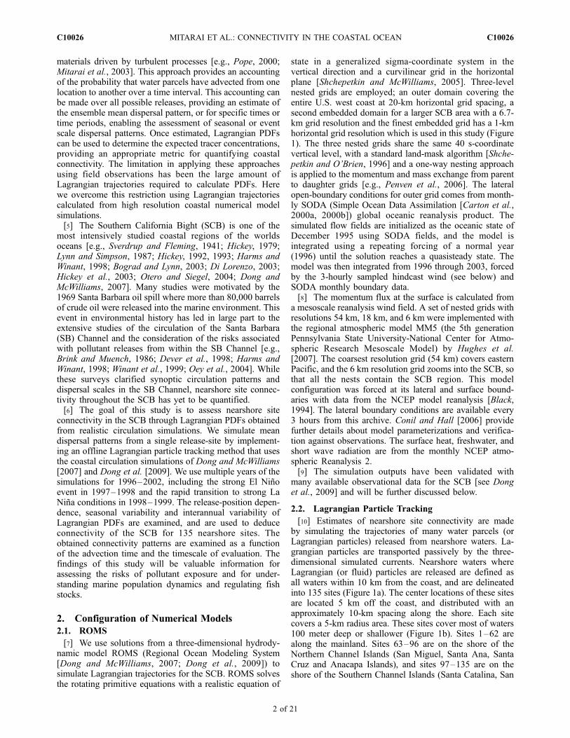
[10] Estimates of nearshore site connectivity are madeby simulating the trajectories of many water parcels (orLagrangian particles) released from nearshore waters. La-grangian particles are transported passively by the three-dimensional simulated currents. Nearshore waters whereLagrangian (or fluid) particles are released are defined asall waters within 10 km from the coast, and are delineatedinto 135 sites (Figure 1a). The center locations of these sitesare located 5 km off the coast, and distributed with anapproximately 10-km spacing along the shore. Each sitecovers a 5-km radius area. These sites cover most of waters100 meter deep or shallower (Figure 1b). Sites 1–62 arealong the mainland. Sites 63–96 are on the shore of theNorthern Channel Islands (San Miguel, Santa Ana, SantaCruz and Anacapa Islands), and sites 97–135 are on theshore of the Southern Channel Islands (Santa Catalina, San

C10026 MITARAI ET AL.: CONNECTIVITY IN THE COASTAL OCEAN

2 of 21

C10026

Clemente, San Nicholas and Santa Barbara). Sixty nine toeighty Lagrangian particles are released from each site nearthe top surface (5 meters below the surface) every 12 hoursfrom 1 January 1996 through 31 December 2002, uniformlyover the site. The total number of Lagrangian particlesreleased from each site is 352,866–409,120, and sufficientto resolve spatial patterns of Lagrangian PDFs and theresulting connectivity (see below).[11] Fluid particle properties (e.g., position, velocity,

material concentrations, etc) can be expressed as functionsof the initial position a and advection time t [Corrsin, 1962;Pope, 2000]. The position of the nth (realization of) fluidparticle, Xn(t, a), evolves as

@

@tXn t; að Þ ¼ Un t; að Þ; ð1Þ

where Un(t, a) indicates the velocity of the nth Lagrangianparticle. The particle velocity is determined by evaluatingthe Eulerian flow fields at the particle’s location,

Un t; að Þ ¼ u Xn t; að Þ; tn þ t½ �; ð2Þ

where u(x, t) is the Eulerian velocity at a given location xand time t, and tn indicates the release time of the nthLagrangian particle. Lagrangian particles are tracked byintegrating equations (1) and (2) using a fourth-orderAdams-Bashford-Moulton predictor-corrector scheme [e.g.,Carr et al., 2008; Durran, 1999], given the initial location,Xn(0, a) = a. The Eulerian velocity at a given particlelocation is estimated through linear interpolation of thediscrete velocity fields. We tracked Lagrangian particleswith a 15-minute time step for 120 days or until they crossthe boundaries.

2.3. Estimating Lagrangian PDFs and QuantifyingCoastal Connectivity

[12] A Lagrangian PDF describes the probability densityfunction of particle displacement for a given advection

time t. A discrete representation of Lagrangian PDFs,f 0X(x; t, a), can be determined as

f 0X x; t; að Þ ¼ 1

N

XNn¼1

d Xn t; að Þ � xð Þ; ð3Þ

where N is the total number of Lagrangian particles, d is theDirac delta function, and x is the sample space variable forX. We focus only on the evaluation of f 0X (x; t, a) in thehorizontal directions. Discrete Lagrangian PDFs are eval-uated from the center location of the sites defined above,averaged over each site, i.e.,

f 0X x; t; að Þ � 1

pR2

Zrj j�R

f 0X x; t; aþ rð Þdr; ð4Þ

where R is the radius of each site (5 km). A LagrangianPDF, denoted as fX(x; t, a), is given by spatially filtering adiscrete PDF in the sample space, i.e.,

fX x; t; að Þ �Z 1�1

G x� xð Þ f 0X x; t; að Þdx; ð5Þ

where G(x � x) is an isotropic Gaussian filter with astandard deviation of 4 km. Values of a Lagrangian PDFrepresent the number of particles in km�2.[13] Lagrangian PDFs can be utilized to describe expected

dispersal patterns of materials, neglecting molecular diffu-sion and chemical reactions, given the initial distributions ofmaterial concentrations, c(x, t0). The expected concentrationof the materials after a time interval t, hc(x, t0 + t)i, can bedetermined as

c x; t0 þ tð Þh i ¼Z 1�1

c a; t0ð Þ fX x; t; að Þda: ð6Þ

This states that the expected concentration at a point is theinitial concentration carried by a particle times theprobability of the particle being there, integrated over all

Figure 1. (a) Site locations used for the assessment of Lagrangian probability density functions andcoastal connectivity. The red dots indicate the center location of each site. The blue circles indicate thearea covered by each site (with a 5-km radius). The numbers indicate a given site number. The sites arecategorized into three regional groups, i.e., along the mainland (sites 1–62; from south to north),Northern Channel Islands (sites 63–96), and Southern Channel Islands (sites 97–135). (b) Modelbathymetry. Colors indicate water depths in meters. The while dashed line indicates the 100-m isobath.The full model domain is shown.


3 of 21

C10026

particles that could be there [Tennekes and Lumley, 1972].Different observation times can be assessed by changing thetime of release enabling both the assessment of a singlerelease at different time and over particular timescales (i.e.,a given year or season or ensemble of seasons). The effectsof turbulent mixing and chemical (biological) reactions ofmaterials in altering dispersal patterns are discussed inAppendix A.[14] Coastal connectivity is defined as the probability a

water parcel leaving a source site j arrives a destination site iover a time interval t, and is denoted here as Cji(t). Valuesof Cji(t) are evaluated from the Lagrangian PDF for asource location (xj) and a destination location (xi) as

Cji tð Þ ¼ fX x ¼ xi; t; a ¼ xj� �

pR2� �

; ð7Þ

where the normalization by pR2 converts probabilitydensities to probabilities. Connectivity matrices describethe probability for the event that a water parcel is transportedfrom site j to site i. Based upon the site locations shown inFigure 1, this results in a 135� 135 matrix, Cji(t), which wedefine here as the connectivity matrix. Connectivity matricesare a function of the advection time t. We evaluateLagrangian PDFs and resulting connectivity matrices fort = 1, 2, . . ., 120 days, and use t = 30 days as a defaultcase.[15] Values of the destination strength, Di(t), measure the

relative ‘‘attractiveness’’ of site i for all of the Lagrangianparticles released in the domain for a release time of t. Di(t)

is calculated by summing the connectivity matrix over allsource sites in the domain, i.e.,

Di tð Þ ¼Xj� J

Cji tð Þ; J ¼ j1; j2; :::; jN ð8Þ

Similarly, the source strength, Sj(t), which measures therelative success that a site’s particles encounter another sitewithin a timescale t, can be calculated as

Sj tð Þ ¼Xi�I

Cji tð Þ; I ¼ i1; i2; :::; iM ð9Þ

Distributions of source and destination strength are usefulfor helping illustrate features of the calculated connectivitymatrices.

3. Lagrangian PDFs in the Southern CaliforniaBight

3.1. Turbulent Dispersion and Examples of ExpectedDispersal Patterns

[16] Lagrangian trajectories for particles released off SanNicholas Island (site 130) illustrate the quasichaotic natureof turbulent transport in the coastal ocean (Figure 2). Thesimulated trajectories clearly show sensitivity to the date ofrelease. For example, many Lagrangian particles releasedfrom this site on 31 January 1996 are transported toward thenortheast and after 30 days are found relatively close to thesites between the Northern and Southern Channel Islands

Figure 2. Sample Lagrangian particle trajectories from a single site. These Lagrangian particles arereleased in the nearshore of San Nicholas Island (yellow circles; site 130), on (a) 1 January 1996, (b) 16January 1996, (c) 31 January 1996, and (d) 15 February 1996, and are transported passively by thesimulated flow fields. The blue lines indicate simulated 30-day trajectories. The red dots indicate theparticle locations 30 days after the release. The full model domain is shown.


4 of 21

C10026

(Figure 2c). However, many of those released just twoweeks later (15 February 1996; Figure 2d), are transportedpoleward along the mainland coast and are found within theSB Channel after 30 days. Differences in the release timesof just two weeks can lead to very different dispersalpatterns. This clearly illustrates the characteristics of aturbulent dispersion problem.[17] Lagrangian length and timescales as well as values of

eddy diffusivity are estimated to validate the simulateddispersal patterns. These are compared with similar statisticsobtained from surface drifter observations for a 5� by 5� boxcentered at 35�N 120�W [Swenson and Niiler, 1996]. Weemploy the definition of eddy diffusivity proposed by Davis[1987] following the approach of Swenson and Niiler[1996]. We find Lagrangian time and length scales of3.6 ± 0.8 days and 32.2 ± 7.1 km, respectively, that corre-spond to an eddy diffusivity of 3.6 ± 1.0� 107 cm2 s�1. Herethe numbers after ± indicate the standard deviation amongrelease sites. Swenson and Niiler [1996] found typical valuesfor the Lagrangian time and length scales of 1.8–6.8 daysand 16–64 km, respectively, while for the eddy diffusivity,1.7–7.0 � 107 cm2 s�1. There is good correspondencebetween Lagrangian statistics obtained from the simulationand the analysis of field observations, strengthening ourconfidence in our simulated dispersal patterns.[18] The Lagrangian PDF statistically describes the

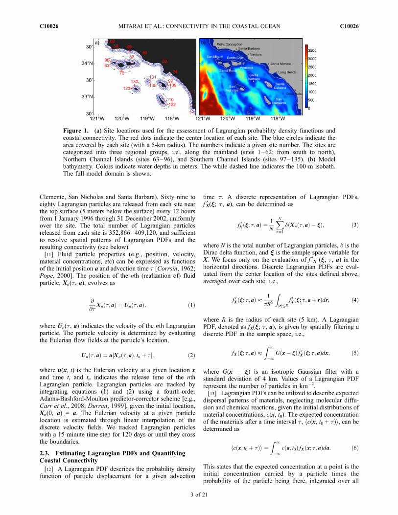
expected locations of water particles that are released froma single site and transported over a given time interval. Forexample, the Lagrangian PDF from a site on San NicholasIsland (site 130) calculated using 7 years of trajectories(1996–2002) is shown in Figure 3. Determinations of the

Lagrangian PDF from this site are roughly isotropic andthey become more homogenous as the advection timebecomes longer (Figure 3). Water parcels from this sitecan reach nearly all of the SCB within 20 days (Figure 3c).For an advection time of 10 days, strong connectivitypatterns are expected to sites on the south side of Anacapaand Santa Cruz Islands, but not on the mainland or NorthernIslands (Figure 3b). For longer advection times, similarlevels of connectivity are expected throughout the SCB(Figure 3d).

3.2. Release-Position Dependence of ExpectedDispersal Patterns

[19] The San Nicholas Island source site (#130; Figure 1a)is relatively isolated from the other Channel Islands and themainland. Lagrangian particle transport is, therefore, lessinfluenced by the complex coastal topography and distinc-tive circulation patterns of the SBC, resulting in a roughlyisotropic Lagrangian PDF (Figure 3). Lagrangian PDFs forreleases from other sites, however, show a strong direction-ality associated with complex coastline and bathymetry ofthe SCB (Figure 4).[20] Simulated mean dispersal patterns can be categorized

into four groups, depending on the release-site location.First, Lagrangian particles released on the mainland sitesshow distinctive nearly unidirectional mean dispersal pat-terns (Figures 4a–4d). The mean poleward transport isobserved from sites between the international border andVentura (site 45), but not from sites in the north of Ventura(Figures 4e–4f). Second, Lagrangian particles releasedfrom sites within the SB Channel tend to stay within the

Figure 3. Lagrangian probability density functions (Lagrangian PDFs) from the site on the shore of SanNicholas Island (black circles; site 130) for the advection time of (a) 1 day, (b) 10 days, (c) 20 days, and(d) 30 days. The Lagrangian PDFs are computed through equations (3)–(5), given all Lagrangian particletrajectories, regardless of the release season and year. Colors indicate the probability density of a particlelocation for a given advection time in km�2.


5 of 21

C10026

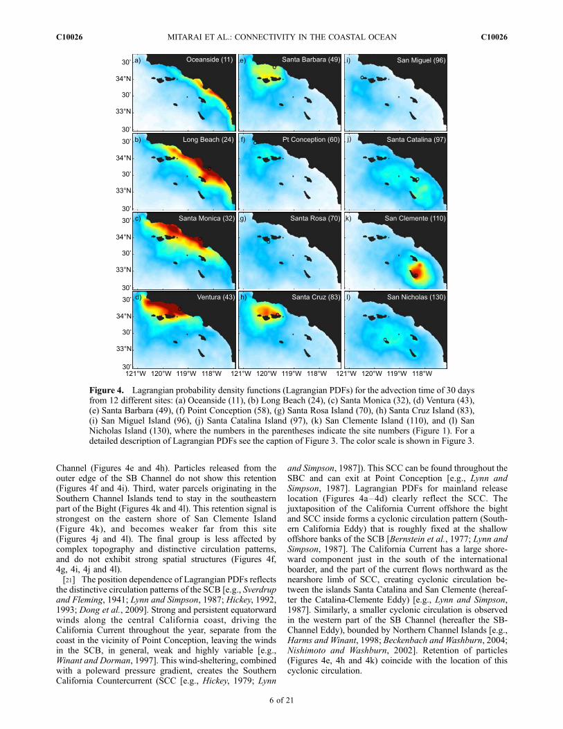
Channel (Figures 4e and 4h). Particles released from theouter edge of the SB Channel do not show this retention(Figures 4f and 4i). Third, water parcels originating in theSouthern Channel Islands tend to stay in the southeasternpart of the Bight (Figures 4k and 4l). This retention signal isstrongest on the eastern shore of San Clemente Island(Figure 4k), and becomes weaker far from this site(Figures 4j and 4l). The final group is less affected bycomplex topography and distinctive circulation patterns,and do not exhibit strong spatial structures (Figures 4f,4g, 4i, 4j and 4l).[21] The position dependence of Lagrangian PDFs reflects

the distinctive circulation patterns of the SCB [e.g., Sverdrupand Fleming, 1941; Lynn and Simpson, 1987; Hickey, 1992,1993; Dong et al., 2009]. Strong and persistent equatorwardwinds along the central California coast, driving theCalifornia Current throughout the year, separate from thecoast in the vicinity of Point Conception, leaving the windsin the SCB, in general, weak and highly variable [e.g.,Winant and Dorman, 1997]. This wind-sheltering, combinedwith a poleward pressure gradient, creates the SouthernCalifornia Countercurrent (SCC [e.g., Hickey, 1979; Lynn

and Simpson, 1987]). This SCC can be found throughout theSBC and can exit at Point Conception [e.g., Lynn andSimpson, 1987]. Lagrangian PDFs for mainland releaselocation (Figures 4a–4d) clearly reflect the SCC. Thejuxtaposition of the California Current offshore the bightand SCC inside forms a cyclonic circulation pattern (South-ern California Eddy) that is roughly fixed at the shallowoffshore banks of the SCB [Bernstein et al., 1977; Lynn andSimpson, 1987]. The California Current has a large shore-ward component just in the south of the internationalboarder, and the part of the current flows northward as thenearshore limb of SCC, creating cyclonic circulation be-tween the islands Santa Catalina and San Clemente (hereaf-ter the Catalina-Clemente Eddy) [e.g., Lynn and Simpson,1987]. Similarly, a smaller cyclonic circulation is observedin the western part of the SB Channel (hereafter the SB-Channel Eddy), bounded by Northern Channel Islands [e.g.,Harms and Winant, 1998; Beckenbach and Washburn, 2004;Nishimoto and Washburn, 2002]. Retention of particles(Figures 4e, 4h and 4k) coincide with the location of thiscyclonic circulation.

Figure 4. Lagrangian probability density functions (Lagrangian PDFs) for the advection time of 30 daysfrom 12 different sites: (a) Oceanside (11), (b) Long Beach (24), (c) Santa Monica (32), (d) Ventura (43),(e) Santa Barbara (49), (f) Point Conception (58), (g) Santa Rosa Island (70), (h) Santa Cruz Island (83),(i) San Miguel Island (96), (j) Santa Catalina Island (97), (k) San Clemente Island (110), and (l) SanNicholas Island (130), where the numbers in the parentheses indicate the site numbers (Figure 1). For adetailed description of Lagrangian PDFs see the caption of Figure 3. The color scale is shown in Figure 3.


6 of 21

C10026

[22] Within the SB Channel, Lagrangian PDFs show thehighest value at Chinese Harbor (site 83) on the northeast-ern side of Santa Cruz Island. This is where surface-driftersdeployed in the SBC often run aground [e.g., Winant et al.,1999]. These high PDF values are not caused by thebeaching of particles as only 0.2% of the released waterparcels ran aground.

3.3. Seasonal and Interannual Variability of ExpectedDispersal Patterns

[23] Circulation patterns in the SCB show strong season-ality, driven by variability in wind-forcing and alongshorepressure gradients [Lynn and Simpson, 1987; Di Lorenzo,2003]. During winter, the wind stress within the bight isweaker, spatially homogeneous and temporally variable;during summer, the wind-forcing is stronger and morepersistent with large spatial gradients [Winant and Dorman,1997; Dong et al., 2009]. The core of the California Currentis strongest in spring and summer, and tends to be closerinshore [Bograd et al., 2000]. The juxtaposition of theCalifornia Current and SCC (and the Southern California

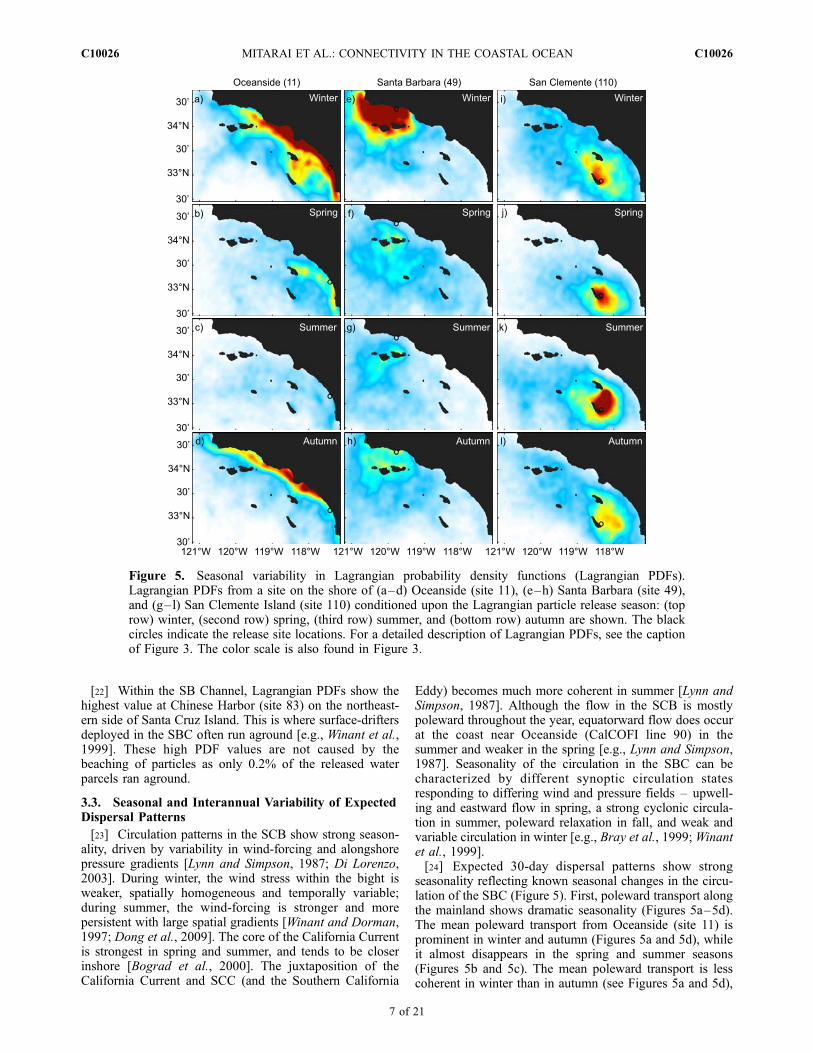
Eddy) becomes much more coherent in summer [Lynn andSimpson, 1987]. Although the flow in the SCB is mostlypoleward throughout the year, equatorward flow does occurat the coast near Oceanside (CalCOFI line 90) in thesummer and weaker in the spring [e.g., Lynn and Simpson,1987]. Seasonality of the circulation in the SBC can becharacterized by different synoptic circulation statesresponding to differing wind and pressure fields – upwell-ing and eastward flow in spring, a strong cyclonic circula-tion in summer, poleward relaxation in fall, and weak andvariable circulation in winter [e.g., Bray et al., 1999;Winantet al., 1999].[24] Expected 30-day dispersal patterns show strong

seasonality reflecting known seasonal changes in the circu-lation of the SBC (Figure 5). First, poleward transport alongthe mainland shows dramatic seasonality (Figures 5a–5d).The mean poleward transport from Oceanside (site 11) isprominent in winter and autumn (Figures 5a and 5d), whileit almost disappears in the spring and summer seasons(Figures 5b and 5c). The mean poleward transport is lesscoherent in winter than in autumn (see Figures 5a and 5d),

Figure 5. Seasonal variability in Lagrangian probability density functions (Lagrangian PDFs).Lagrangian PDFs from a site on the shore of (a–d) Oceanside (site 11), (e–h) Santa Barbara (site 49),and (g–l) San Clemente Island (site 110) conditioned upon the Lagrangian particle release season: (toprow) winter, (second row) spring, (third row) summer, and (bottom row) autumn are shown. The blackcircles indicate the release site locations. For a detailed description of Lagrangian PDFs, see the captionof Figure 3. The color scale is also found in Figure 3.


7 of 21

C10026

because of the temporally variable wind-forcing in winter.Second, regional retention in the SB Channel is dominant inwinter, while this signal is hardly seen in other seasons(Figures 5e–5h) when upwelling and eastward flow dom-inates [e.g., Dever et al., 1998; Winant et al., 1999]. Thisimplies that Lagrangian particles tend to stay in the Channelsimply because the particle transport is limited due to weakand variable flows, and not because SB cyclonic eddyretains particles [e.g., Nishimoto and Washburn, 2002].Finally, regional retention of Lagrangian particles off theeastern shore of San Clemente Island shows much lessseasonal variability (Figures 5i–5l) than is observed for theother retention zones shown here (Figures 5a–5h). Theretention off San Clemente Island is consistently seenthroughout all seasons (Figure 5), showing only moderateseasonal variability.[25] Strong interannual changes in the circulation of the

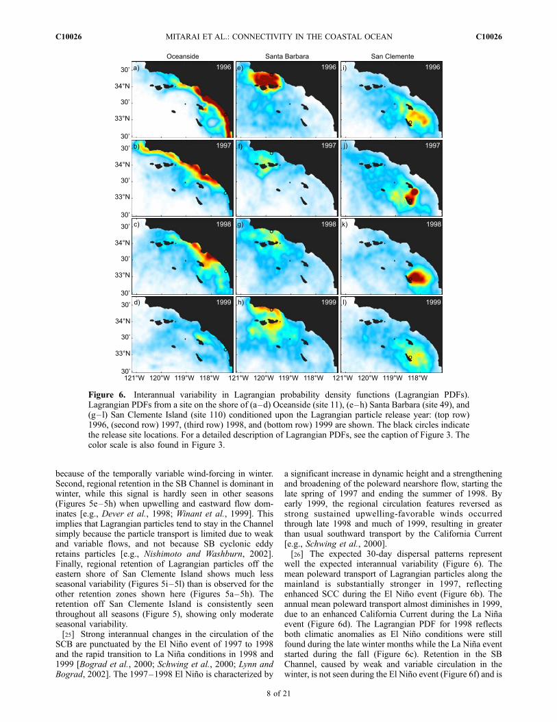
SCB are punctuated by the El Nino event of 1997 to 1998and the rapid transition to La Nina conditions in 1998 and1999 [Bograd et al., 2000; Schwing et al., 2000; Lynn andBograd, 2002]. The 1997–1998 El Nino is characterized by

a significant increase in dynamic height and a strengtheningand broadening of the poleward nearshore flow, starting thelate spring of 1997 and ending the summer of 1998. Byearly 1999, the regional circulation features reversed asstrong sustained upwelling-favorable winds occurredthrough late 1998 and much of 1999, resulting in greaterthan usual southward transport by the California Current[e.g., Schwing et al., 2000].[26] The expected 30-day dispersal patterns represent

well the expected interannual variability (Figure 6). Themean poleward transport of Lagrangian particles along themainland is substantially stronger in 1997, reflectingenhanced SCC during the El Nino event (Figure 6b). Theannual mean poleward transport almost diminishes in 1999,due to an enhanced California Current during the La Ninaevent (Figure 6d). The Lagrangian PDF for 1998 reflectsboth climatic anomalies as El Nino conditions were stillfound during the late winter months while the La Nina eventstarted during the fall (Figure 6c). Retention in the SBChannel, caused by weak and variable circulation in thewinter, is not seen during the El Nino event (Figure 6f) and is

Figure 6. Interannual variability in Lagrangian probability density functions (Lagrangian PDFs).Lagrangian PDFs from a site on the shore of (a–d) Oceanside (site 11), (e–h) Santa Barbara (site 49), and(g–l) San Clemente Island (site 110) conditioned upon the Lagrangian particle release year: (top row)1996, (second row) 1997, (third row) 1998, and (bottom row) 1999 are shown. The black circles indicatethe release site locations. For a detailed description of Lagrangian PDFs, see the caption of Figure 3. Thecolor scale is also found in Figure 3.


8 of 21

C10026

reduced for La Nina periods (Figure 6h). The retentivenature of the SB Channel is greatest during 1996, whichis a ‘‘normal’’ year (Figure 6e). During an El Nino (LaNina) event, the relaxation (upwelling) circulation state isenhanced and poleward (equatorward) flow becomes stron-ger. For either case, more Lagrangian particles are exportedfrom the SB Channel (Figures 6f–6h). This result is consis-tent with the analysis of remote observations of phytoplank-ton chlorophyll concentrations in the SB Channel whichshow high concentrations during ‘‘normal’’ years comparedwith the El Nino or La Nina years [Otero and Siegel, 2004].Retention features off the eastern shore of the San ClementeIsland are relatively insensitive to the year of evaluation(Figures 6i–6l) although retention appears to be more sub-stantial during the El Nino (Figures 6j and 6k).

4. Coastal Connectivity of the SouthernCalifornia Bight

4.1. Quantifying Connectivity Matrices

[27] Coastal connectivity can be quantified by evaluatingthe simulated Lagrangian PDFs for a given source and agiven destination (equation (7)) and is most readily expressed

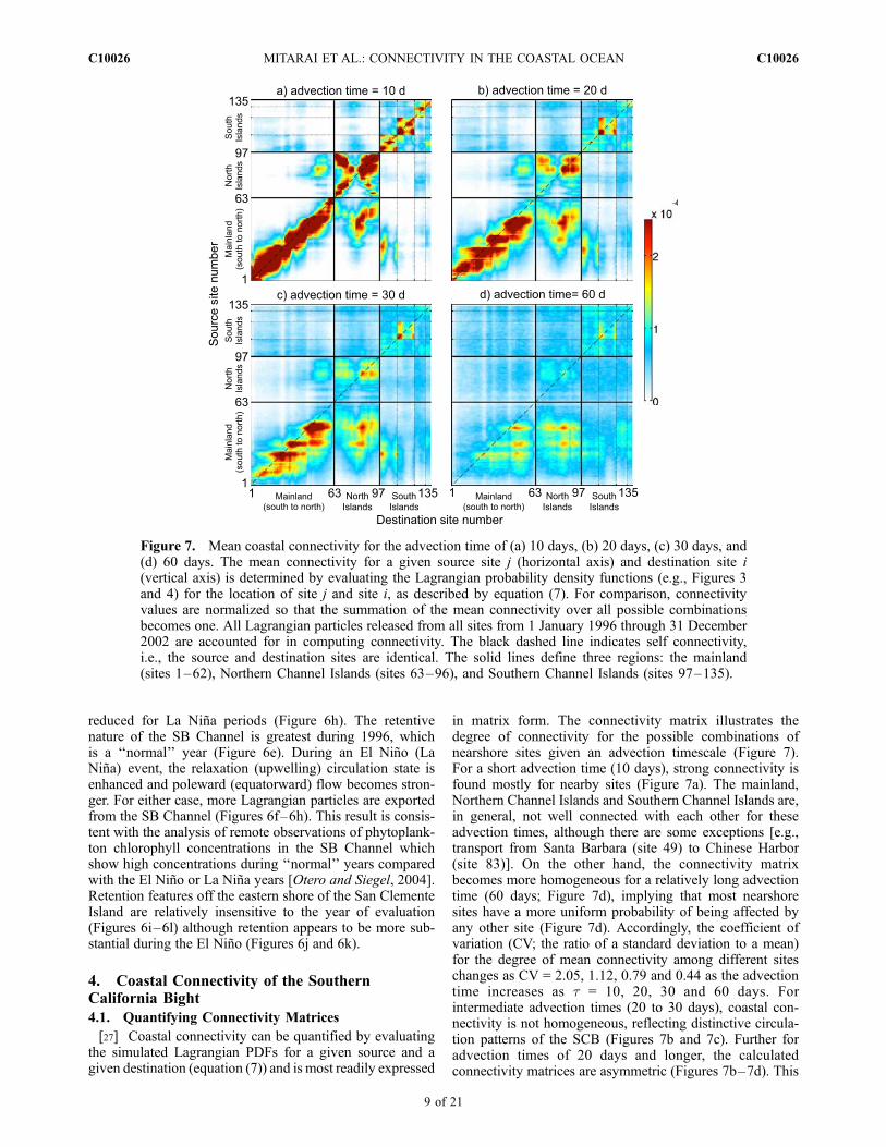
in matrix form. The connectivity matrix illustrates thedegree of connectivity for the possible combinations ofnearshore sites given an advection timescale (Figure 7).For a short advection time (10 days), strong connectivity isfound mostly for nearby sites (Figure 7a). The mainland,Northern Channel Islands and Southern Channel Islands are,in general, not well connected with each other for theseadvection times, although there are some exceptions [e.g.,transport from Santa Barbara (site 49) to Chinese Harbor(site 83)]. On the other hand, the connectivity matrixbecomes more homogeneous for a relatively long advectiontime (60 days; Figure 7d), implying that most nearshoresites have a more uniform probability of being affected byany other site (Figure 7d). Accordingly, the coefficient ofvariation (CV; the ratio of a standard deviation to a mean)for the degree of mean connectivity among different siteschanges as CV = 2.05, 1.12, 0.79 and 0.44 as the advectiontime increases as t = 10, 20, 30 and 60 days. Forintermediate advection times (20 to 30 days), coastal con-nectivity is not homogeneous, reflecting distinctive circula-tion patterns of the SCB (Figures 7b and 7c). Further foradvection times of 20 days and longer, the calculatedconnectivity matrices are asymmetric (Figures 7b–7d). This

Figure 7. Mean coastal connectivity for the advection time of (a) 10 days, (b) 20 days, (c) 30 days, and(d) 60 days. The mean connectivity for a given source site j (horizontal axis) and destination site i(vertical axis) is determined by evaluating the Lagrangian probability density functions (e.g., Figures 3and 4) for the location of site j and site i, as described by equation (7). For comparison, connectivityvalues are normalized so that the summation of the mean connectivity over all possible combinationsbecomes one. All Lagrangian particles released from all sites from 1 January 1996 through 31 December2002 are accounted for in computing connectivity. The black dashed line indicates self connectivity,i.e., the source and destination sites are identical. The solid lines define three regions: the mainland(sites 1–62), Northern Channel Islands (sites 63–96), and Southern Channel Islands (sites 97–135).


9 of 21

C10026

implies that the direction of the connection among sites isimportant beyond just knowing the distance between sites(as would occur in a purely diffusive environment).

4.2. Source and Destination Strength Distributions

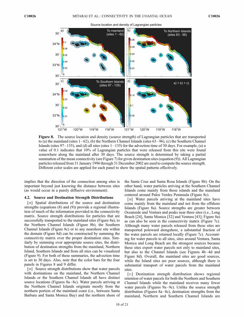
[28] Spatial distributions of the source and destinationstrengths (equations (8) and (9)) provide a regional illustra-tion of much of the information provided in the connectivitymatrix. Source strength distributions for particles that aresuccessfully transported to the mainland sites (Figure 8a), tothe Northern Channel Islands (Figure 8b), the SouthernChannel Islands (Figure 8c) or to any nearshore site withinthe domain (Figure 8d) can be constructed by summing theconnectivity matrix over the proper destination sites. Sim-ilarly by summing over appropriate source sites, the distri-bution of destination strengths from the mainland, NorthernIsland, Southern Islands and from all sties can be visualized(Figure 9). For both of these summaries, the advection timeis set to 30 days. Also, note that the color bars for the fourpanels in Figures 8 and 9 differ.[29] Source strength distributions show that water parcels

with destinations on the mainland, the Northern ChannelIslands or the Southern Channel Islands all have distinctsource locations (Figures 8a–8c). Water parcels arriving atthe Northern Channel Islands originate mostly from thenorthern portion of the mainland coast (i.e., between SantaBarbara and Santa Monica Bay) and the northern shore of

the Santa Cruz and Santa Rosa Islands (Figure 8b). On theother hand, water particles arriving at the Southern ChannelIslands come mainly from those islands and the mainlandcentered around Palos Verdes Peninsula (Figure 8c).[30] Water parcels arriving at the mainland sites have

come mainly from the mainland and not from the offshoreIslands (Figure 8a). Source strengths are greater betweenOceanside and Ventura and peaks near three sites (i.e., LongBeach [24], Santa Monica [32] and Ventura [43]; Figure 8a)as can also be seen in the connectivity matrix (Figure 7c).Although many water parcels released from these sites aretransported poleward alongshore, a substantial fraction ofthe water parcels are retained locally (Figure 7c). Account-ing for water parcels to all sites, sites around Ventura, SantaMonica and Long Beach are the strongest sources becausethese sites export water parcels not only to mainland sites,but also to the Channel Islands (see Figures 4b–4d andFigure 8d). Overall, the mainland sites are good sources,while the Island sites are poor sources, although there issubstantial transport of water parcels from the mainlandsites.[31] Destination strength distribution shows regional

retention of water parcels for both the Northern and SouthernChannel Islands while the mainland receives many fewerwater parcels (Figures 9a–9c). Unlike the source strengthdistribution (Figures 8a–8c), destination strengths from themainland, Northern and Southern Channel Islands are

Figure 8. The source location and density (source strength) of Lagrangian particles that are transportedto (a) the mainland (sites 1–62), (b) the Northern Channel Islands (sites 63–96), (c) the Southern ChannelIslands (sites 97–135), and (d) all sites (sites 1–135) for the advection time of 30 days. For example, (a) avalue of 0.1 indicates that 10% of Lagrangian particles that were released from this site were foundsomewhere along the mainland after 30 days. The source strength is determined by taking a partialsummation of the mean connectivity (see Figure 7) for given destination sites (equation (9)). All Lagrangianparticles released from 31 January 1996 through 31December 2002 are used to compute the source strength.Different color scales are applied for each panel to show the spatial patterns effectively.


10 of 21

C10026

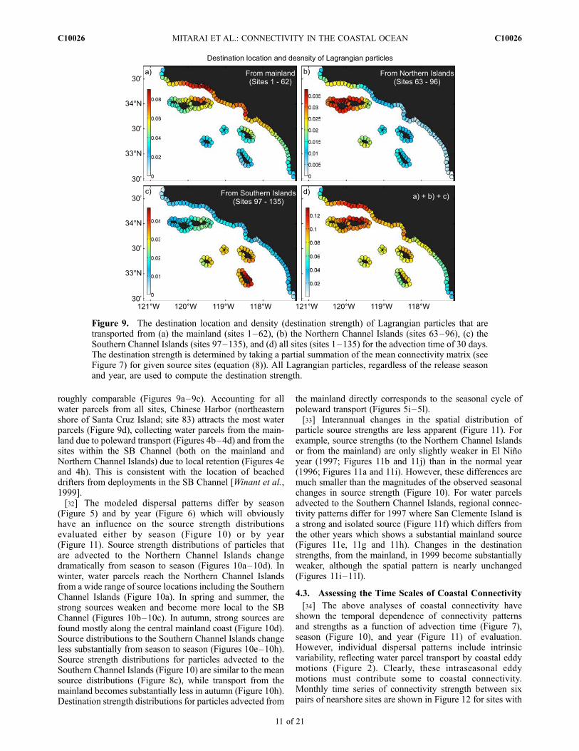
roughly comparable (Figures 9a–9c). Accounting for allwater parcels from all sites, Chinese Harbor (northeasternshore of Santa Cruz Island; site 83) attracts the most waterparcels (Figure 9d), collecting water parcels from the main-land due to poleward transport (Figures 4b–4d) and from thesites within the SB Channel (both on the mainland andNorthern Channel Islands) due to local retention (Figures 4eand 4h). This is consistent with the location of beacheddrifters from deployments in the SB Channel [Winant et al.,1999].[32] The modeled dispersal patterns differ by season

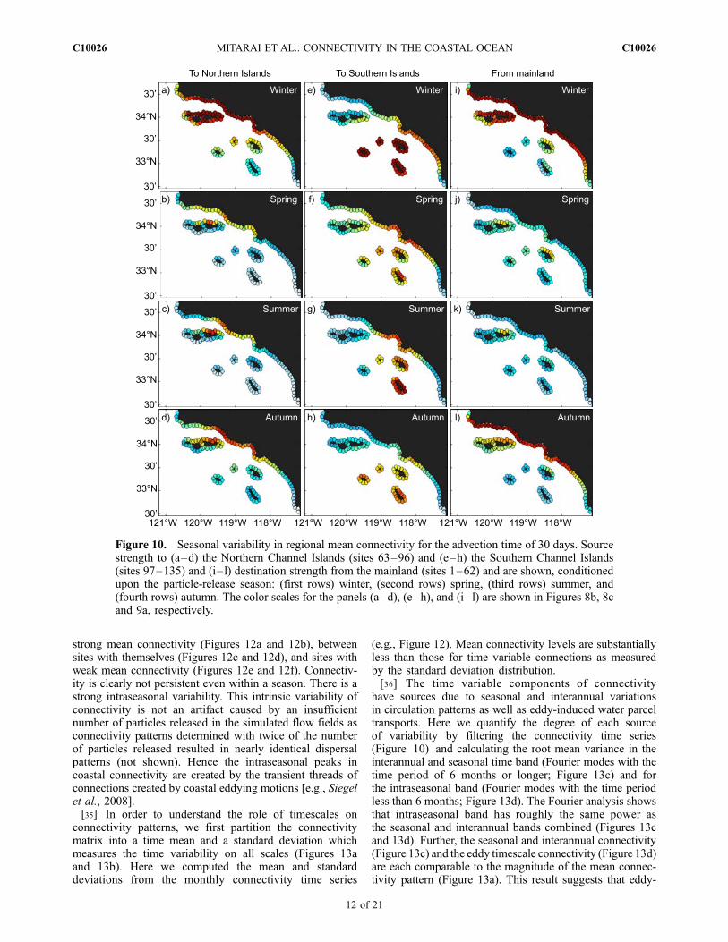
(Figure 5) and by year (Figure 6) which will obviouslyhave an influence on the source strength distributionsevaluated either by season (Figure 10) or by year(Figure 11). Source strength distributions of particles thatare advected to the Northern Channel Islands changedramatically from season to season (Figures 10a–10d). Inwinter, water parcels reach the Northern Channel Islandsfrom a wide range of source locations including the SouthernChannel Islands (Figure 10a). In spring and summer, thestrong sources weaken and become more local to the SBChannel (Figures 10b–10c). In autumn, strong sources arefound mostly along the central mainland coast (Figure 10d).Source distributions to the Southern Channel Islands changeless substantially from season to season (Figures 10e–10h).Source strength distributions for particles advected to theSouthern Channel Islands (Figure 10) are similar to the meansource distributions (Figure 8c), while transport from themainland becomes substantially less in autumn (Figure 10h).Destination strength distributions for particles advected from

the mainland directly corresponds to the seasonal cycle ofpoleward transport (Figures 5i–5l).[33] Interannual changes in the spatial distribution of

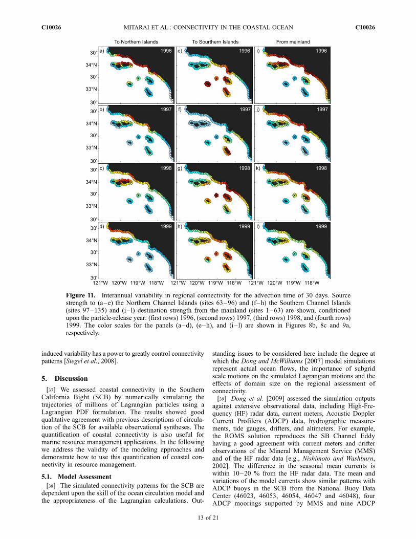
particle source strengths are less apparent (Figure 11). Forexample, source strengths (to the Northern Channel Islandsor from the mainland) are only slightly weaker in El Ninoyear (1997; Figures 11b and 11j) than in the normal year(1996; Figures 11a and 11i). However, these differences aremuch smaller than the magnitudes of the observed seasonalchanges in source strength (Figure 10). For water parcelsadvected to the Southern Channel Islands, regional connec-tivity patterns differ for 1997 where San Clemente Island isa strong and isolated source (Figure 11f) which differs fromthe other years which shows a substantial mainland source(Figures 11e, 11g and 11h). Changes in the destinationstrengths, from the mainland, in 1999 become substantiallyweaker, although the spatial pattern is nearly unchanged(Figures 11i–11l).

4.3. Assessing the Time Scales of Coastal Connectivity

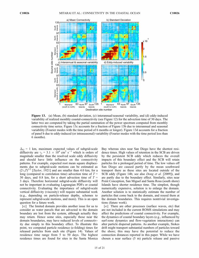
[34] The above analyses of coastal connectivity haveshown the temporal dependence of connectivity patternsand strengths as a function of advection time (Figure 7),season (Figure 10), and year (Figure 11) of evaluation.However, individual dispersal patterns include intrinsicvariability, reflecting water parcel transport by coastal eddymotions (Figure 2). Clearly, these intraseasonal eddymotions must contribute some to coastal connectivity.Monthly time series of connectivity strength between sixpairs of nearshore sites are shown in Figure 12 for sites with

Figure 9. The destination location and density (destination strength) of Lagrangian particles that aretransported from (a) the mainland (sites 1–62), (b) the Northern Channel Islands (sites 63–96), (c) theSouthern Channel Islands (sites 97–135), and (d) all sites (sites 1–135) for the advection time of 30 days.The destination strength is determined by taking a partial summation of the mean connectivity matrix (seeFigure 7) for given source sites (equation (8)). All Lagrangian particles, regardless of the release seasonand year, are used to compute the destination strength.


11 of 21

C10026

strong mean connectivity (Figures 12a and 12b), betweensites with themselves (Figures 12c and 12d), and sites withweak mean connectivity (Figures 12e and 12f). Connectiv-ity is clearly not persistent even within a season. There is astrong intraseasonal variability. This intrinsic variability ofconnectivity is not an artifact caused by an insufficientnumber of particles released in the simulated flow fields asconnectivity patterns determined with twice of the numberof particles released resulted in nearly identical dispersalpatterns (not shown). Hence the intraseasonal peaks incoastal connectivity are created by the transient threads ofconnections created by coastal eddying motions [e.g., Siegelet al., 2008].[35] In order to understand the role of timescales on

connectivity patterns, we first partition the connectivitymatrix into a time mean and a standard deviation whichmeasures the time variability on all scales (Figures 13aand 13b). Here we computed the mean and standarddeviations from the monthly connectivity time series

(e.g., Figure 12). Mean connectivity levels are substantiallyless than those for time variable connections as measuredby the standard deviation distribution.[36] The time variable components of connectivity

have sources due to seasonal and interannual variationsin circulation patterns as well as eddy-induced water parceltransports. Here we quantify the degree of each sourceof variability by filtering the connectivity time series(Figure 10) and calculating the root mean variance in theinterannual and seasonal time band (Fourier modes with thetime period of 6 months or longer; Figure 13c) and forthe intraseasonal band (Fourier modes with the time periodless than 6 months; Figure 13d). The Fourier analysis showsthat intraseasonal band has roughly the same power asthe seasonal and interannual bands combined (Figures 13cand 13d). Further, the seasonal and interannual connectivity(Figure 13c) and the eddy timescale connectivity (Figure 13d)are each comparable to the magnitude of the mean connec-tivity pattern (Figure 13a). This result suggests that eddy-

Figure 10. Seasonal variability in regional mean connectivity for the advection time of 30 days. Sourcestrength to (a–d) the Northern Channel Islands (sites 63–96) and (e–h) the Southern Channel Islands(sites 97–135) and (i–l) destination strength from the mainland (sites 1–62) and are shown, conditionedupon the particle-release season: (first rows) winter, (second rows) spring, (third rows) summer, and(fourth rows) autumn. The color scales for the panels (a–d), (e–h), and (i–l) are shown in Figures 8b, 8cand 9a, respectively.


12 of 21

C10026

induced variability has a power to greatly control connectivitypatterns [Siegel et al., 2008].

5. Discussion

[37] We assessed coastal connectivity in the SouthernCalifornia Bight (SCB) by numerically simulating thetrajectories of millions of Lagrangian particles using aLagrangian PDF formulation. The results showed goodqualitative agreement with previous descriptions of circula-tion of the SCB for available observational syntheses. Thequantification of coastal connectivity is also useful formarine resource management applications. In the followingwe address the validity of the modeling approaches anddemonstrate how to use this quantification of coastal con-nectivity in resource management.

5.1. Model Assessment

[38] The simulated connectivity patterns for the SCB aredependent upon the skill of the ocean circulation model andthe appropriateness of the Lagrangian calculations. Out-

standing issues to be considered here include the degree atwhich the Dong and McWilliams [2007] model simulationsrepresent actual ocean flows, the importance of subgridscale motions on the simulated Lagrangian motions and theeffects of domain size on the regional assessment ofconnectivity.[39] Dong et al. [2009] assessed the simulation outputs

against extensive observational data, including High-Fre-quency (HF) radar data, current meters, Acoustic DopplerCurrent Profilers (ADCP) data, hydrographic measure-ments, tide gauges, drifters, and altimeters. For example,the ROMS solution reproduces the SB Channel Eddyhaving a good agreement with current meters and drifterobservations of the Mineral Management Service (MMS)and of the HF radar data [e.g., Nishimoto and Washburn,2002]. The difference in the seasonal mean currents iswithin 10–20 % from the HF radar data. The mean andvariations of the model currents show similar patterns withADCP buoys in the SCB from the National Buoy DataCenter (46023, 46053, 46054, 46047 and 46048), fourADCP moorings supported by MMS and nine ADCP

Figure 11. Interannual variability in regional connectivity for the advection time of 30 days. Sourcestrength to (a–e) the Northern Channel Islands (sites 63–96) and (f–h) the Southern Channel Islands(sites 97–135) and (i–l) destination strength from the mainland (sites 1–63) are shown, conditionedupon the particle-release year: (first rows) 1996, (second rows) 1997, (third rows) 1998, and (fourth rows)1999. The color scales for the panels (a–d), (e–h), and (i–l) are shown in Figures 8b, 8c and 9a,respectively.


13 of 21

C10026

moorings deployed by Los Angeles County SanitationDistrict except those close to the open boundaries (46047and 46048). The mean differences are at the level of severalcm s�1 or tens of percent of the signal, and the standarddeviation ratio is within a few tens of percent of unity. Themagnitudes and structural patterns (such as thermocline andthermohaline depth) of temperature and salinity fromROMS and the California Cooperative Oceanic Fisheriesand Investigations (CalCOFI) data agree fairly well eachother, within about 1–2�C and 0.2 psu, respectively. Acomparison of the temperature time series at three MMSstations in the SB Channel [Lynn and Bograd, 2002; Deverand Winant, 2002] with the ROMS simulation shows thatthe temperature increases dramatically in late 1997 throughearly 1998 with almost the same magnitude and timing.Further detailed analysis against more observations can befound in Dong et al. [2009]. Comparisons with observa-tional data reveal that ROMS reproduces a realistic meanstate of the SCB oceanic circulation, as well as itsinterannual and seasonal variability.[40] One way to further validate the model connectivity is

through quantitative Lagrangian validations. As the firststep, we computed Lagrangian time and length scales andeddy diffusivities, and found a reasonable agreement with

observations of Swenson and Niiler [1996], as mentionedabove. This agreement supports the ROMS model indescribing mesoscale eddy motions.[41] The neglect of diffusion by subgrid-scale motions in

Lagrangian trajectory calculations can lead to underestima-tion of the scales of dispersal. Values of eddy diffusivityscale as u02l, where l is the scale of motion and u02 is twiceits kinetic energy. Lagrangian time and length scales for thepresent simulations are 3.6 ± 0.8 days and 32.2 ± 7.1 km,respectively and correspond to an eddy diffusivity of 3.6 ±1.0 � 107 cm2 s�1. Both the u2 and l associated withsubgrid-scale eddies are much smaller than those of meso-scale motions. Values of subgrid-scale eddy diffusivity, forinstance, can be quantified by using the Smagorinsky model[Smagorinsky, 1993] as

gt ¼ CsDGð Þ2ffiffiffiffiffiffiffiffiffiffiffiffiffiffiffiffiffiffiffiffiffiSij� �

lSij� �

l

qð10Þ

where DG is the grid scale, Cs is an empirical constant,and hSijil is resolved strain rate tensor. Maximum values ofthe horizontal strain rate in the SBC are close to Coriolisfrequency f = 7.7 � 105 s�1 [Beckenbach and Washburn,2004; Dong and McWilliams, 2007]. Given Cs = 0.2 and

Figure 12. Time series of monthly connectivity between a given source site j and a given destinationsite i for the advection time of 30 days. The bars indicate the probability for the event that a particlereleased from site j in a particular month of a particular year are transported to site i. The red line indicatesthe mean connectivity. Panels indicate connectivity (a) from Santa Barbara (49) to Santa Cruz Island (83),(b) from Ventura (43) to Santa Cruz Island (83), (c) from Santa Monica (32) to itself, (d) from Santa CruzIsland (83) to itself, (e) from San Miguel Island (96) to San Nicholas Island (130) and (f) from SantaCatalina Island (97) to San Nicholas Island (130). The numbers in the parentheses indicate the sitenumbers (see Figure 1).


14 of 21

C10026

DG = 1 km, maximum expected values of subgrid-scalediffusivity are gt = 3.1 � 104 cm2 s�1 which is orders ofmagnitude smaller than the resolved scale eddy diffusivityand should have little influence on the connectivitypatterns. For example, expected root mean square displace-ments due to subgrid-scale motions can be estimated as(2gtT)

1/2 [Taylor, 1921] and are smaller than 4.0 km, for along (compared to correlation time) advection time of T =30 days, and 0.8 km, for a short advection time of T =3 days. Therefore horizontal subgrid-scale diffusivity willnot be important in evaluating Lagrangian PDFs or coastalconnectivity. Evaluating the importance of subgrid-scalevertical diffusivity (viscosity) will require substantial work(e.g., depending on particle-release depths, schemes torepresent subgrid-scale motions, and more). This is an openquestion for a future work.[42] The limited domain provides another issue for us to

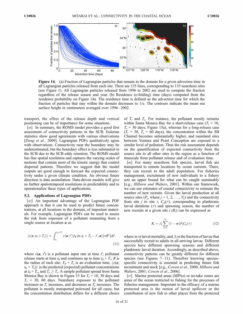
consider as water parcels that are advected to the domainboundary are lost from the system, although actually theymay return. Hence some sites, especially those near thedomain boundaries, may have reduced levels of connectiv-ity due simply to this boundary effect. To illustrate thispoint, we computed particle residence (e-folding) times forreleased particles from each site (Figure 14). Values ofresidence time range from 5 to 50 days. The highestresidence times are found for sites in the Santa Monica

Bay whereas sites near San Diego have the shortest resi-dence times. High values of retention in the SCB are drivenby the persistent SCB eddy which reduces the overallimpacts of this boundary effect and the SCB will retainparticles for a prolonged period of time. The low values offSan Diego are caused partly by the mean southwardtransport there as these sites are located outside of theSCB eddy (Figure 14b; see also Dong et al. [2009]), andare partly due to the boundary effect. Similarly, sites nearPoint Conception, San Miguel and Santa Rosa (south shore)Islands have shorter residence time. The simplest, thoughnumerically expensive, solution is to enlarge the domain.Another solution is to statistically estimate the number ofparticles that come back to the domain, and reseed them atthe domain boundaries. This requires nontrivial investiga-tions (future work).[43] There are other processes (surface waves, etc) that

are not included in the current ROMS simulations and mayaffect the predictions of coastal connectivity. For example,the dynamics of coastal boundary layers (e.g., influenced bysurf-zone dynamics and flow-vegetation interactions) canalter particle dispersal patterns. As another example, Stokesdrift might transport substantial numbers of particles towardthe shore; this may have the potential to reduce theconnection distances reported in this paper. While we havechosen a near surface (5 m) particle release and passive

Figure 13. (a) Mean, (b) standard deviation, (c) interannual/seasonal variability, and (d) eddy-inducedvariability of realized monthly coastal-connectivity (see Figure 12) for the advection time of 30 days. Thelatter two are computed by taking the partial summation of the power spectrum computed from monthlyconnectivity time series. Figure 13c accounts for a fraction of Figure 13b due to interannual and seasonalvariability (Fourier modes with the time period of 6 months or longer). Figure 13d accounts for a fractionof panel b due to eddy-induced (or intraseasonal) variability (Fourier modes with the time period less than6 months).


15 of 21

C10026

transport, the effect of the release depth and verticalpositioning can be of importance for some situations.[44] In summary, the ROMS model provides a good first

assessment of connectivity patterns in the SCB. Eulerianstatistics show good agreements with various observations[Dong et al., 2009]. Lagrangian PDFs qualitatively agreewith observations. Connectivity near the boundary may beunderestimated, but the boundary effect is less substantial inthe SCB due to the SCB eddy retention. The ROMS modelhas fine spatial resolution and captures the varying scales ofmotions that contain most of the kinetic energy that controldispersal patterns. Therefore we suggest that the modeloutputs are good enough to forecast the expected connec-tivity under a given climate condition. An obvious futuredirection is data assimilation. Data-driven models will giveus further spatiotemporal resolutions in predictability and tooperationalize these types of applications.

5.2. Applications of Lagrangian PDFs

[45] An important advantage of the Lagrangian PDFapproach is that it can be used to predict future concen-trations, at all locations in the domain, of important materi-als. For example, Lagrangian PDFs can be used to assessthe risk from exposure of a pollutant emanating from asingle source at location a as

c x; t0 þ Teð Þh i ¼Z t0þTr

t0

_c a; t0ð Þ fX x; t0 þ Te � t0; að Þ pR2� �

dt0:

ð11Þ

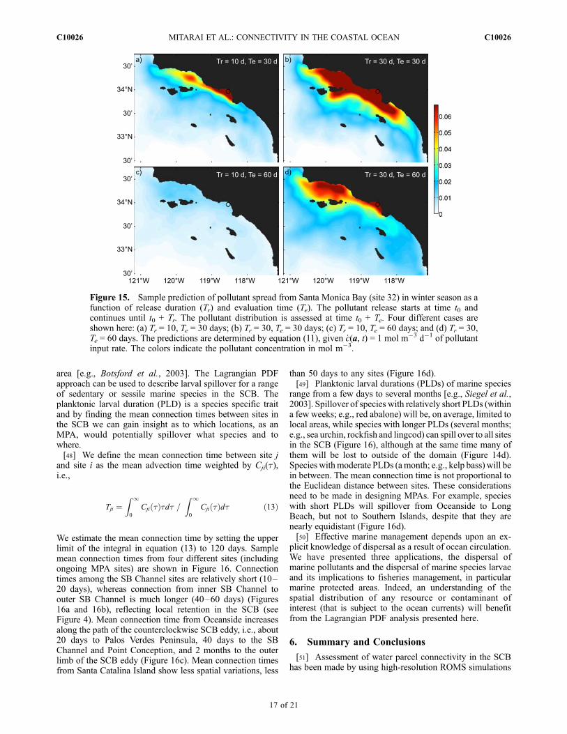
where _c(a, t0) is a pollutant input rate at time t0; pollutantrelease starts at time t0 and continues up to time t0 + Tr; R isthe radius of each site; T0 + Te is an evaluation time; hc(x,t0 + Te)i is the predicted (expected) pollutant concentrationsat t0 + Te, and Te � Tr. A sample pollutant spread from SantaMonica Bay is shown in Figure 15 for Tr = 10, 30 days andTe = 30, 60 days. Nearshore exposure to the pollutantincreases as Tr increases, and decreases as Te increases. Thepollutant is mostly transported poleward for all cases, butthe concentration distribution differs for a different choice

of Tr and Te. For instance, the pollutant mostly remainswithin Santa Monica Bay for a short-release case (Tr = 10,Te = 30 days; Figure 15a), whereas for a long-release case(Tr = 30, Te = 60 days), the concentration within the SBChannel becomes substantially higher, and mainland sitesbetween Ventura and Point Conception are exposed to asimilar level of pollution. Thus the risk assessment dependson the quantification of expected connectivity from thesource site to all other sites in the region as a function oftimescale from pollutant release and of evaluation time.[46] For many nearshore fish species, larval fish are

transported to remote locations by ocean currents. There,they can recruit to the adult population. For fisheriesmanagement, recruitment of new individuals to a fisherysets an upper bound for what can be caught sustainably[e.g., Hilborn and Walters, 2001]. Within our framework,we can use estimates of coastal connectivity to estimate thenumber of new recruits. Given the larval production at allsource sites (Pj, where j = 1, 2, . . ., Nj) and the connectivityfrom site j to site i, Cji(t), corresponding to planktoniclarval durations (t) and spawning season, the number ofnew recruits at a given site i (Ri) can be expressed as

Ri ¼ bi

XNj

j¼11� mð ÞPjCji tð Þ ð12Þ

where m is larval mortality, and bi is the fraction of larvae thatsuccessfully recruit to adults in all arriving larvae. Differentspecies have different spawning seasons and differentplanktonic larval duration. Accordingly, as described above,connectivity patterns can be greatly different for differentspecies (see Figures 7–11). Therefore knowing species-specific connectivity is essential in predicting future fishrecruitment and stock [e.g., Cowen et al., 2000; Hilborn andWalters, 2001; Cowen et al., 2006].[47] Marine protected areas (MPAs) or no-take zones are

areas of the ocean restricted to fishing for the processes offisheries management. Important to the efficacy of a marineprotected area is the notion of larval spillover or thecontribution of new fish to other places from the protected

Figure 14. (a) Fraction of Lagrangian particles that remain in the domain for a given advection time inall Lagrangian particles released from each site. There are 135 lines, corresponding to 135 nearshore sites(see Figure 1). All Lagrangian particles released from 1996 to 2002 are used to compute the fractionregardless of the release season and year. (b) Residence (e-folding) time (days) computed from theresidence probability on Figure 14a. The residence time is defined as the advection time for which thefraction of particles that stay within the domain decreases to 1/e. The contours indicate the mean seasurface height in centimeters averaged over 1996–2002.


16 of 21

C10026

area [e.g., Botsford et al., 2003]. The Lagrangian PDFapproach can be used to describe larval spillover for a rangeof sedentary or sessile marine species in the SCB. Theplanktonic larval duration (PLD) is a species specific traitand by finding the mean connection times between sites inthe SCB we can gain insight as to which locations, as anMPA, would potentially spillover what species and towhere.[48] We define the mean connection time between site j

and site i as the mean advection time weighted by Cji(t),i.e.,

Tji ¼Z 10

Cji tð Þtdt =Z 10

Cji tð Þdt ð13Þ

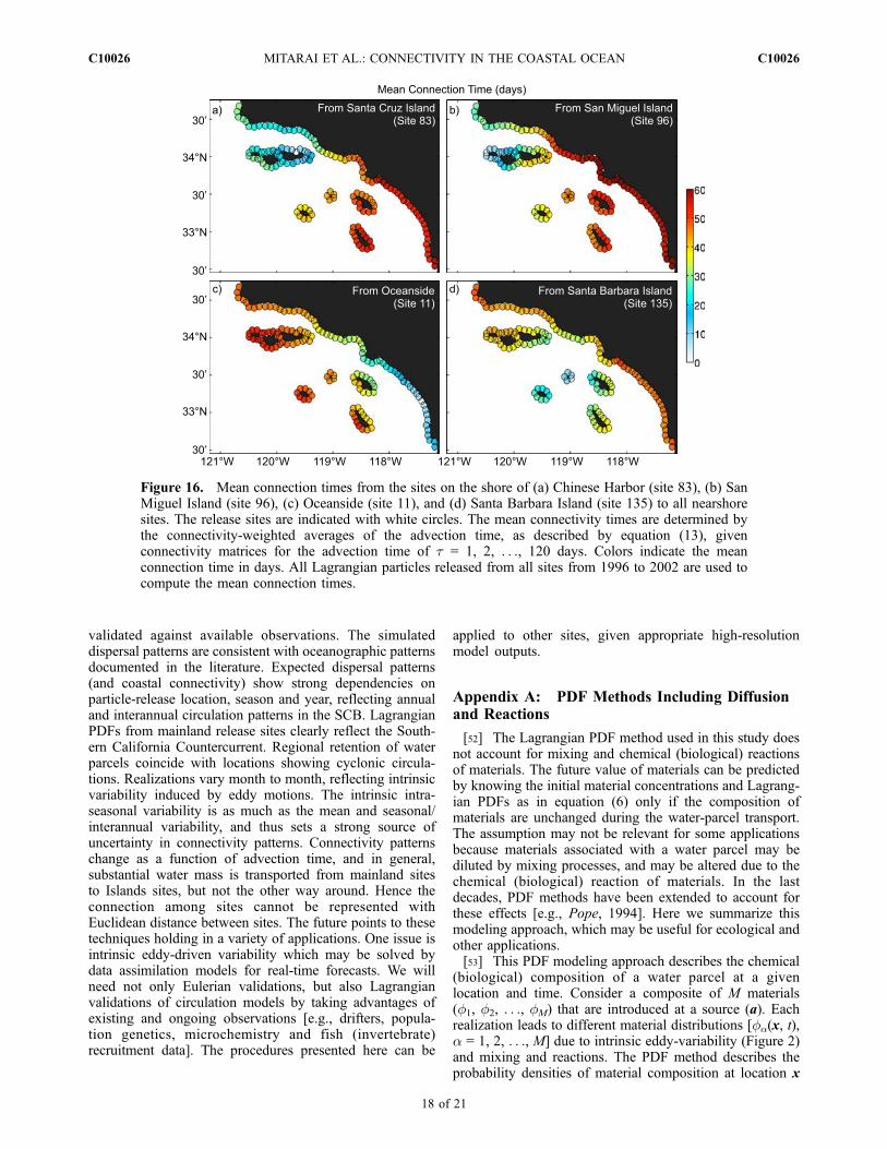
We estimate the mean connection time by setting the upperlimit of the integral in equation (13) to 120 days. Samplemean connection times from four different sites (includingongoing MPA sites) are shown in Figure 16. Connectiontimes among the SB Channel sites are relatively short (10–20 days), whereas connection from inner SB Channel toouter SB Channel is much longer (40–60 days) (Figures16a and 16b), reflecting local retention in the SCB (seeFigure 4). Mean connection time from Oceanside increasesalong the path of the counterclockwise SCB eddy, i.e., about20 days to Palos Verdes Peninsula, 40 days to the SBChannel and Point Conception, and 2 months to the outerlimb of the SCB eddy (Figure 16c). Mean connection timesfrom Santa Catalina Island show less spatial variations, less

than 50 days to any sites (Figure 16d).[49] Planktonic larval durations (PLDs) of marine species

range from a few days to several months [e.g., Siegel et al.,2003]. Spillover of species with relatively short PLDs (withina few weeks; e.g., red abalone) will be, on average, limited tolocal areas, while species with longer PLDs (several months;e.g., sea urchin, rockfish and lingcod) can spill over to all sitesin the SCB (Figure 16), although at the same time many ofthem will be lost to outside of the domain (Figure 14d).Species withmoderate PLDs (amonth; e.g., kelp bass) will bein between. The mean connection time is not proportional tothe Euclidean distance between sites. These considerationsneed to be made in designing MPAs. For example, specieswith short PLDs will spillover from Oceanside to LongBeach, but not to Southern Islands, despite that they arenearly equidistant (Figure 16d).[50] Effective marine management depends upon an ex-

plicit knowledge of dispersal as a result of ocean circulation.We have presented three applications, the dispersal ofmarine pollutants and the dispersal of marine species larvaeand its implications to fisheries management, in particularmarine protected areas. Indeed, an understanding of thespatial distribution of any resource or contaminant ofinterest (that is subject to the ocean currents) will benefitfrom the Lagrangian PDF analysis presented here.

6. Summary and Conclusions

[51] Assessment of water parcel connectivity in the SCBhas been made by using high-resolution ROMS simulations

Figure 15. Sample prediction of pollutant spread from Santa Monica Bay (site 32) in winter season as afunction of release duration (Tr) and evaluation time (Te). The pollutant release starts at time t0 andcontinues until t0 + Tr. The pollutant distribution is assessed at time t0 + Te. Four different cases areshown here: (a) Tr = 10, Te = 30 days; (b) Tr = 30, Te = 30 days; (c) Tr = 10, Te = 60 days; and (d) Tr = 30,Te = 60 days. The predictions are determined by equation (11), given _c(a, t) = 1 mol m�3 d�1 of pollutantinput rate. The colors indicate the pollutant concentration in mol m�3.


17 of 21

C10026

validated against available observations. The simulateddispersal patterns are consistent with oceanographic patternsdocumented in the literature. Expected dispersal patterns(and coastal connectivity) show strong dependencies onparticle-release location, season and year, reflecting annualand interannual circulation patterns in the SCB. LagrangianPDFs from mainland release sites clearly reflect the South-ern California Countercurrent. Regional retention of waterparcels coincide with locations showing cyclonic circula-tions. Realizations vary month to month, reflecting intrinsicvariability induced by eddy motions. The intrinsic intra-seasonal variability is as much as the mean and seasonal/interannual variability, and thus sets a strong source ofuncertainty in connectivity patterns. Connectivity patternschange as a function of advection time, and in general,substantial water mass is transported from mainland sitesto Islands sites, but not the other way around. Hence theconnection among sites cannot be represented withEuclidean distance between sites. The future points to thesetechniques holding in a variety of applications. One issue isintrinsic eddy-driven variability which may be solved bydata assimilation models for real-time forecasts. We willneed not only Eulerian validations, but also Lagrangianvalidations of circulation models by taking advantages ofexisting and ongoing observations [e.g., drifters, popula-tion genetics, microchemistry and fish (invertebrate)recruitment data]. The procedures presented here can be

applied to other sites, given appropriate high-resolutionmodel outputs.

Appendix A: PDF Methods Including Diffusionand Reactions

[52] The Lagrangian PDF method used in this study doesnot account for mixing and chemical (biological) reactionsof materials. The future value of materials can be predictedby knowing the initial material concentrations and Lagrang-ian PDFs as in equation (6) only if the composition ofmaterials are unchanged during the water-parcel transport.The assumption may not be relevant for some applicationsbecause materials associated with a water parcel may bediluted by mixing processes, and may be altered due to thechemical (biological) reaction of materials. In the lastdecades, PDF methods have been extended to account forthese effects [e.g., Pope, 1994]. Here we summarize thismodeling approach, which may be useful for ecological andother applications.[53] This PDF modeling approach describes the chemical

(biological) composition of a water parcel at a givenlocation and time. Consider a composite of M materials(f1, f2, . . ., fM) that are introduced at a source (a). Eachrealization leads to different material distributions [fa(x, t),a = 1, 2, . . ., M] due to intrinsic eddy-variability (Figure 2)and mixing and reactions. The PDF method describes theprobability densities of material composition at location x

Figure 16. Mean connection times from the sites on the shore of (a) Chinese Harbor (site 83), (b) SanMiguel Island (site 96), (c) Oceanside (site 11), and (d) Santa Barbara Island (site 135) to all nearshoresites. The release sites are indicated with white circles. The mean connectivity times are determined bythe connectivity-weighted averages of the advection time, as described by equation (13), givenconnectivity matrices for the advection time of t = 1, 2, . . ., 120 days. Colors indicate the meanconnection time in days. All Lagrangian particles released from all sites from 1996 to 2002 are used tocompute the mean connection times.


18 of 21

C10026

and time t, denoted here as ff(y; x, t), where y = (y1, y2,. . ., yM) is the sample space variable for material concen-trations. This approach is essentially an extension of equa-tion (6) to multiple reactive materials.[54] There exists a technique to derive a governing

equation for the composition PDF from a fundamentaladvection-diffusion-reaction equation [e.g., Pope, 1985].The evolution of material composition can be expressed,for instance, as

@fa

@tþ @uifa

@xi¼ @

@xik@fa

@xi

� �þ wa fð Þ ðA1Þ

where a = 1, 2, . . ., M identifies each material (species),ui(x, t) is the Eulerian velocity, k is the diffusion coefficient,and wa(f) is the reaction term for material a, which is afunction of all materials. In this case, the composition PDFor ff(y; x, t) obeys

@ff@tþ @ uijyh iff

@xi¼@ kr2fajy� �

ff

@ya� @wa ff

@yaðA2Þ

where huijyi and hkr2fajyi are, respectively, the ensemble-average of ui(x, t) and kr2fa(x, t) conditional upon a set ofcomposition values f(x, t) = y.[55] The composition PDF equation is not closed, and

requires modeling of the two conditional means, in terms ofvelocity and diffusion. A variety of physically sound modelshave been developed for the unclosed terms [e.g., Pope,1985; Chen et al., 1989; Colucci et al., 1998; Mitarai et al.,2003]. For example, following Colucci et al. [1998],

@ff@tþ @ uih iff

@xi¼ @

@xikþ ktð Þ @ff

@xi

� �þ @W ya � fah ið Þ ff

@ya

� @wa ff

@ya; ðA3Þ

where W is a mixing frequency constant [Pope, 2000] andkt is eddy diffusivity, and the bracket hi is an ensemble-averaging operator. By taking the first moment of thisequation, we obtain the mean composition equation, i.e.,

@ fah i@tþ @ uih i fah i

@xi¼ @

@xikþ ktð Þ @ fah i

@xi

� �þ wa fð Þh i: ðA4Þ

The same exact equation can be obtained from equation (A1)by using a conventional modeling approach, i.e., taking anensemble average of both sides of the equation and assuminghuifai = ktrfa(x, t) [e.g., LaCasce, 2008]. Note thatequation (A4) requires the modeling of the mean reactionterm, whereas equation (A3) does not.[56] The closed composition-PDF equation, equation (A3),

can be integrated directly, but it usually requires muchcomputational resources. Alternatively, the composite-PDFevolution equation can be indirectly integrated throughMonte Carlo simulations of an equivalent stochastic particle

system, which can be obtained through the Fokker-Planckformalism [e.g., Gardiner, 1997] as

dX*i ¼ uih i þ@ kþ ktð Þ

@xi

dt þ 2 kþ ktð Þ½ �1=2dWi; ðA5Þ

dfa*

dt¼ W f*a � fah i

� �þ wa f*ð Þ: ðA6Þ

where X* and f*a, respectively, indicate the position andcomposition of a stochastic particle; and Wi is the Wienerprocess [e.g., Gardiner, 1997]. The composition PDF, ff(y;x, t), can be obtained by making a histogram of thecomposition of the particles within a specified area centeredat x (e.g., a numerical grid cell) or as in equation (5).Similarly, the mean composition, hfa(x, t)i, can be given asthe mean particle composition.[57] Theoretically, Lagrangian PDFs shown in study

(Figures 3–6) can be reproduced using the stochasticparticle equation (equation (A5)), given the mean velocityfields and eddy diffusivity deduced from the ROMS modelor by other means (e.g., climatology estimated from obser-vations). Lagrangian PDFs can be determined by countingthe number of stochastic particles found within a definedarea similarly to equation (4). This modeling approach isnumerically much less expensive than Lagrangian particletracking methods, because it does not require a series offlow fields, but only statistics. The effects of mixing andreactions, if necessarily, can be assessed by integratingequation (A6) at the same time. In this study, we did notemploy equation (A5) since the prediction depends on themodeling accuracy of the unclosed terms and estimates ofeddy diffusivity. The model predictability has been tested inengineering applications, e.g., against direct numerical sim-ulations of Navier-Stokes equations of chemically reactingturbulent flows [e.g., Colucci et al., 1998; Mitarai et al.,2003] and piloted turbulent diffusion flame experiments[e.g., Lindstedt et al., 2000], but not yet for oceanographicflows.

[58] Acknowledgments. The authors acknowledge a series ofenlightening discussions with Steven Gaines, Bob Warner, Chris Costello,Bruce Kendall, Libe Washburn, Carter Ohlmann, Jenn Caselle, BrianKinlan, Tim Chaffey, and Crow White. We thank Eileen Idica for aidingin many aspects of this work. This work was supported by the NationalScience Foundation (NSF grant 0308440, OCE 06-23011), CaliforniaCoastal Conservancy (04078.05LA), University of California CoastalEnvironmental Quality Initiative, National Oceanic and AtmosphericAdministration (NA17RJ1231), National Aeronautics and Space Administra-tion (NNX08AI84G), and USGS/EPA project.

ReferencesBeckenbach, E., and L. Washburn (2004), Low-frequency waves in theSanta Barbara Channel observed by high-frequency radar, J. Geophys.Res., 109, C02010, doi:10.1029/2003JC001999.

Bernstein, R., L. Breaker, and R. Whritner (1977), California Current eddyformation: Ship, air, and satellite results, Science, 195(4276), 353–359.

Black, T. (1994), The new NMC mesoscale eta-model: Description andforecast examples, Weather Forecast., 9(2), 265–278.

Bograd, S., and R. Lynn (2003), Long-term variability in the SouthernCalifornia Current System, Deep Sea Res., Part II, 50(14–16), 2355–2370, doi:10.1016/S0967-0645(03)00131-0.


19 of 21

C10026

Bograd, S., et al. (2000), The state of the California Current, 1999–2000:Forward to a new regime?, Calif. Coop. Ocean. Fish. Invest. Rep., 41,26–52.

Botsford, L., F. Micheli, and A. Hastings (2003), Principles for the designof marine reserves, Ecol. App., 13(1), S25–S31.

Bray, N. A., A. Keyes, and W. M. L. Morawitz (1999), The CaliforniaCurrent system in the Southern California Bight and the Santa BarbaraChannel, J. Geophys. Res., 104(C4), 7695–7714.

Brink, K., and R. Muench (1986), Circulation in the Point ConceptionSanta-Barbara Channel region, J. Geophys. Res., 91(C1), 877–895.

Carr, S. D., X. J. Capet, J. C. McWilliams, J. T. Pennington, and F. P.Chavez (2008), The influence of diel vertical migration on zooplanktontransport and recruitment in an upwelling region: Estimates from acoupled behavioral-physical model, Fish. Oceanogr., 17(1), 1 – 15,doi:10.1111/j.1365-2419.2007.00447.x.

Carton, J., G. Chepurin, and X. Cao (2000a), A simple ocean dataassimilation analysis of the global upper ocean 1950–95: Part II.Results, J. Phys. Oceanogr., 30(2), 311–326.

Carton, J., G. Chepurin, X. Cao, and B. Giese (2000b), A simple ocean dataassimilation analysis of the global upper ocean 1950–95: Part I.Methodology, J. Phys. Oceanogr., 30(2), 294–309.

Chen, H., S. Chen, and R. Kraichnan (1989), Probability-distribution of astochastically advected scalar field, Phys. Rev. Lett., 63(24), 2657–2660.

Colucci, P., F. Jaberi, P. Givi, and S. Pope (1998), Filtered density functionfor large eddy simulation of turbulent reacting flows, Phys. Fluids, 10(2),499–515.

Conil, S., and A. Hall (2006), Local regimes of atmospheric variability: Acase study of southern California, J. Clim., 19(17), 4308–4325.

Corrsin, S. (1962), Theories of turbulent dispersion, in Mechanique de laTurbulence, pp. 27–52, CNRS, Paris.

Cowen, R., K. Lwiza, S. Sponaugle, C. Paris, and D. Olson (2000), Con-nectivity of marine populations: Open or closed?, Science, 287(5454),857–859.

Cowen, R., C. Paris, and A. Srinivasan (2006), Scaling of connectivity inmarine populations, Science, 311(5760), 522 – 527, doi:10.1126/science.1122039.

Davis, R. (1987), Modeling eddy transport of passive tracers, J. Mar. Res.,45(3), 635–666.

Dever, E., and C. Winant (2002), The evolution and depth structure of shelfand slope temperatures and velocities during the 1997–1998 El Ninonear Point Conception, California, Prog. Oceanogr., 54(1–4), 77–103,doi:10.1016/S0079-6611(02)00044-7.

Dever, E., M. Hendershott, and C. Winant (1998), Statistical aspects ofsurface drifter observations of circulation in the Santa Barbara Channel,J. Geophys. Res., 103(C11), 24,781–24,797.

Di Lorenzo, E. (2003), Seasonal dynamics of the surface circulation in theSouthern California Current System, Deep Sea Res., Part II, 50(14–16),2371–2388, doi:10.1016/S0967-0645(03)00125-5.

Dong, C., and J. C. McWilliams (2007), A numerical study of island wakesin the Southern California Bight, Cont. Shelf Res., 27(9), 1233–1248,doi:10.1016/j.csr.2007.01.016.

Dong, C., E. Idica, and J. McWilliams (2009), Circulation and multi-scalevariability in the Southern California Bight, Prog. Oceanogr.,doi:10.1016/j.pocean.2009.07.005, in press.

Durran, D. R. (1999), Numerical Methods for Wave Equations in Geophy-sical Fluid Dynamics, Springer, New York.

Fischer, H. B., J. E. List, R. C. Koh, J. Imberger, and N. H. Brooks (1979),Mixing in Inland and Coastal Waters, Academic Press, New York.

Gaines, S., B. Gaylord, and J. Largier (2003), Avoiding current oversightsin marine reserve design, Ecol. Appl., 13(1), S32–S46.

Gardiner, C. W. (1997), Handbook of Stochastic Methods for Physics,Chemistry and the Natural Sciences, Springer, Berlin, Germany.

Grant, S., J. Kim, B. Jones, S. Jenkins, J. Wasyl, and C. Cudaback (2005),Surf zone entrainment, along-shore transport, and human health implica-tions of pollution from tidal outlets, J. Geophys. Res., 110, C10025,doi:10.1029/2004JC002401.

Harms, S., and C. Winant (1998), Characteristic patterns of the circulationin the Santa Barbara Channel, J. Geophys. Res., 103(C2), 3041–3065.

Hickey, B. (1979), The California Current system: Hypotheses and facts,Prog. Oceanogr., 8, 191–279.

Hickey, B. (1992), Circulation over the Santa-Monica San-Pedro Basin andShelf, Prog. Oceanogr., 30(1–4), 37–115.

Hickey, B. (1993), Physical oceanography, in Ecology of the SouthernCalifornia Bight: A Synthesis and Interpretation, edited by M. D. Dailey,D. J. Reish, and J. W. Anderson, pp. 19–70, Univ. of Calif. Press,Berkeley, Calif.

Hickey, B., E. Dobbins, and S. Allen (2003), Local and remote forcingof currents and temperature in the central Southern California Bight,J. Geophys. Res., 108(C3), 3081, doi:10.1029/2000JC000313.

Hilborn, R., and C. J.Walters (2001),Quantitative Fisheries Stock Assessment:Choice, Dynamics and Uncertainty, Kluwer, Boston, Mass.

Hughes, M., A. Hall, and R. G. Fovell (2007), Dynamical controls on thediurnal cycle of temperature in complex topography, Clim. Dyn., 29(2–3),277–292, doi:10.1007/s00382-007-0239-8.

Jackson, G., and R. Strathmann (1981), Larval mortality from offshoremixing as a link between pre-competent and competent periods ofdevelopment, Am. Nat., 118(1), 16–26.

Kinlan, B., and S. Gaines (2003), Propagule dispersal in marine andterrestrial environments: A community perspective, Ecology, 84(8),2007–2020.

LaCasce, J. H. (2008), Statistics from Lagrangian observations, Prog.Oceanogr., 77(1), 1–29, doi:10.1016/j.pocean.2008.02.002.

Largier, J. (2003), Considerations in estimating larval dispersal distancesfrom oceanographic data, Ecol. App., 13(1), S71–S89.

Lindstedt, R., S. Louloudi, and E. Vaos (2000), Joint scalar probabilitydensity function modeling of pollutant formation in piloted turbulentjet diffusion flames with comprehensive chemistry, Proc. Combust. Inst.,28, 149–156.

Lynn, R., and S. Bograd (2002), Dynamic evolution of the 1997–1999El Nino-La Nina cycle in the southern California Current System,Prog. Oceanogr., 54(1 – 4), 59 – 75, doi:10.1016/S0079-6611(02)00043-5.

Lynn, R., and J. Simpson (1987), The California Current System: Theseasonal variability of its physical characteristics, J. Geophys. Res.,92(C12), 12,947–12,966.

Mitarai, S., J. Riley, and G. Kosaly (2003), A Lagrangian study of scalardiffusion in isotropic turbulence with chemical reaction, Phys. Fluids,15(12), 3856–3866, doi:10.1063/1.1622950.

Nishimoto, M., and L. Washburn (2002), Patterns of coastal eddy circula-tion and abundance of pelagic juvenile fish in the Santa Barbara Channel,California, USA, Mar. Ecol. Prog. Ser., 241, 183–199.

Oey, L., C. Winant, E. Dever, W. Johnson, and D. Wang (2004), A model ofthe near-surface circulation of the Santa Barbara Channel: Comparisonwith observations and dynamical interpretations, J. Phys. Oceanogr.,34(1), 23–43.

Otero, M., and D. Siegel (2004), Spatial and temporal characteristics ofsediment plumes and phytoplankton blooms in the Santa BarbaraChannel, Deep Sea Res., Part II, 51(10–11), 1129–1149, doi:10.1016/j.dsr2.2004.04.004.

Penven, P., L. Debreu, P. Marchesiello, and J. McWilliams (2006), Evalua-tion and application of the ROMS 1-way embedding procedure to thecentral California upwelling system, Ocean Modell., 12(1–2), 157–187,doi:10.1016/j.ocemod.2005.05.002.

Pfeiffer-Herbert, A. S., M. A. McManus, P. T. Raimondi, Y. Chao, andF. Chai (2007), Dispersal of barnacle larvae along the centralcalifornia coast: A modeling study, Limnol. Oceanogr., 52(4),1559–1569.

Pope, S. (1985), PDF methods for turbulent reactive flows, Prog. EnergyCombust. Sci., 11(2), 119–192.

Pope, S. (1994), Lagrangian PDF methods for turbulent flows, Annu. Rev.Fluid Mech., 26, 23–63.

Pope, S. B. (2000), Turbulent Flows, Cambridge Univ. Press, New York.Poulain, P., and P. Niiler (1989), Statistical-analysis of the surface circula-tion in the California Current System using satellite-tracked drifters,J. Phys. Oceanogr., 19(10), 1588–1603.

Roughgarden, J., S. Gaines, and H. Possingham (1988), Recruitmentdynamics in complex life-cycles, Science, 241(4872), 1460–1466.

Shchepetkin, A., and J. McWilliams (2005), The regional oceanic modelingsystem (ROMS): A split-explicit, free-surface, topography-following-coordinate oceanic model, Ocean Modell., 9(4), 347–404, doi:10.1016/j.ocemod.2004.08.002.

Shchepetkin, A., and J. O’Brien (1996), A physically consistent formula-tion of lateral friction in shallow-water equation ocean models, Mon.Weather Rev., 124(6), 1285–1300.

Schwing, F., C. Moore, S. Ralston, and K. Sakuma (2000), Record coastalupwelling in the California Current in 1999, Calif. Coop. Ocean. Fish.Invest. Rep., 41, 148–160.

Siegel, D., B. Kinlan, B. Gaylord, and S. Gaines (2003), Lagrangiandescriptions of marine larval dispersion, Mar. Ecol. Prog. Ser., 260,83–96.

Siegel, D. A., S. Mitarai, C. J. Costello, S. D. Gaines, B. E. Kendall, R. R.Warner, and K. B. Winters (2008), The stochastic nature of larvalconnectivity among nearshore marine populations, Proc. Natl. Acad.Sci. U. S. A., 105(26), 8974–8979, doi:10.1073/pnas.0802544105.

Smagorinsky, J. (1993), Some historical remarks on the use of nonlinearviscosities, in Large Eddy Simulation of Complex Engineering and Geo-physical Flows, edited by B. Galperin and S. A. Orszag, pp. 3–36,Cambridge Univ. Press, Cambridge, U. K.


20 of 21

C10026

Sverdrup, H., and R. Fleming (1941), The waters off the coast of SouthernCalifornia, Scripps Ins. Oceanogr. Bull., 4, 261–387.

Swenson, M., and P. Niiler (1996), Statistical analysis of the surfacecirculation of the California Current, J. Geophys. Res., 101(C10),22,631–22,645.

Taylor, G. (1921), Diffusion by continuous movements, Proc. Lond. Math.Soc., 20, 196–202.

Tennekes, H., and J. L. Lumley (1972), A First Course in Turbulence,MIT Press, Cambridge, Mass.

Winant, C., and C. Dorman (1997), Seasonal patterns of surface wind stressand heat flux over the Southern California Bight, J. Geophys. Res.,102(C3), 5641–5653.

Winant, C., D. Alden, E. Dever, K. Edwards, and M. Hendershott (1999),Near-surface trajectories off central and southern California, J. Geophys.Res., 104(C7), 15,713–15,726.

��C. Dong and J. C. McWilliams, Institute of Geophysics and Planetary

Physics, University of California, 405 Hilgard Avenue, Los Angeles, CA90095, USA. ([email protected]; [email protected])S. Mitarai, D. A. Siegel, and J. R. Watson, Institute for Computational

Earth System Science, University of California, 6844 Ellison Hall, SantaBarbara, CA 93106, USA. ([email protected]; [email protected]; [email protected])


21 of 21

C10026

Documents

Quantifying connectivity in the coastal ocean with