Quantifying fault connectivity drilling hazards through simple flow computations Rafael Pires de Lima* and Kurt Marfurt, University of Oklahoma

Summary

Faults can enhance production when confined to the

reservoir and impede production when connected to a nearby

aquifer, such as those that connect the Eagle Ford Shale to

the deeper Edwards Limestone.

These faults constitute geohazards during drilling and a

potential water stringer during production, and hence need

to be avoided at any cost. Many shale resource plays within

the United States lie on or near similar carbonate aquifers

such as “Eagle Ford - Edwards”, some of which are also

karstified.

While faults provide crucial geologic information that can

be critical for reservoir modeling, large surveys may contain

hundreds of faults requiring significant interpretation effort.

We propose a simple image processing algorithm (in

contrast to a more accurate reservoir simulator) with the

potential to highlight those faults that may be connected to

nearby aquifers. We envision coupling this tool with

statistical analysis of water production to identify faults that

are safe to complete and those that need to be avoided.

Introduction

The use of edge detecting algorithms on 3D seismic data

volumes such as coherence is a valuable tool for highlighting

morphological geological features such as channel and

faults.

Gersztenkorn and Marfurt (1999) showed that coherence

may be evaluated based on cross-correlation between the

seismic traces, semblance or with a eigendecomposition of

the seismic data covariance matrix. Höcker and Fehmers

(2002) and Marfurt (2006) proposed a more robust

estimation of dip and azimuth, yielding an increased

resolution of coherence computations (as well as other 3-D

seismic attributes dip and azimuth dependent).

While faults provide crucial geologic information that can

be critical for reservoir modeling, fault picking and

interpretation is a time-consuming activity. Nonetheless,

there has been little effort for a better fault enhancement and

analysis (Machado et al., 2016).

Apart from being a potential conduit for water from

underlaying aquifer and drilling geohazard, collapse features

and faults often provide conductivity for fluid flow and the

presence of these elements may invalidate layers that

otherwise could be used for carbon sequestration.

Our objective is to develop a “quick and dirty” image

processing algorithm (in contrast to a more accurate

reservoir simulator) that will highlight those faults that may

be connected to nearby aquifers. Our next objective will be

to match the results obtained with this image processing tool

with statistical analysis of water production.

Our hypothesis is that faults seen on seismic data will act as

conductors between two sets of horizons – or aquifers – that

will act as sources or sinks.

Mapping the flow would then be sufficient to highlight the

faults that connects both horizons – one source and one sink,

while the unconnected faults should have a weaker response.

We are aware that faults can be “dip sealing” or “dip

leaking” and we understand that the same fault can have

different sealing behavior depending on the lithology.

However, the simplistic approximation that coherence

attributes are proportional to the hydraulic conductivity may

prove itself useful on scenarios where the faults are not

completely characterized. In our simulation, we will also

assume single phase fluid system and no phase

transformation i.e. fluid above bubble point or dew point

pressure.

Methodology

We have assumed that the 3D volumetric result of an edge

detecting attribute such as coherence is representative of

thermal, electrical or hydraulic conductivity. Hence, we can

use these attributes as a proxy of conductivity to simulate the

steady-state flow between two horizons.

The two horizons on this conductivity scheme are: the

aquifer layer (to be modeled as the source) and the reservoir

layer (to be a sink).

We will first calculate the fluid head (ℎ ) using the three-

dimensional steady-state saturated flow equation (Istok,

2013; Harbaugh, 2005):

𝜕

𝜕𝑥(𝐾𝑥

𝜕ℎ

𝜕𝑥)+

𝜕

𝜕𝑦(𝐾𝑦

𝜕ℎ

𝜕𝑦)+

𝜕

𝜕𝑧(𝐾𝑧

𝜕ℎ

𝜕𝑧) = 0, (1)

where 𝐾𝑥, 𝐾𝑦, and 𝐾𝑧 are the conductivities of the media in

the x, y and z coordinate directions. This equation is

commonly used for groundwater flow modeling. Next, we

will calculate the absolute flow q using:

𝐪 = 𝑞𝑥�̂� + 𝑞𝑦�̂� + 𝑞𝑧�̂� = −𝐾𝑥𝜕ℎ

𝜕𝑥�̂� − 𝐾𝑦

𝜕ℎ

𝜕𝑦�̂� − 𝐾𝑥

𝜕ℎ

𝜕𝑧�̂�, (2)

© 2017 SEG SEG International Exposition and 87th Annual Meeting

Page 2345

Dow

nloa

ded

10/0

6/17

to 1

29.1

5.66

.178

. Red

istr

ibut

ion

subj

ect t

o SE

G li

cens

e or

cop

yrig

ht; s

ee T

erm

s of

Use

at h

ttp://

libra

ry.s

eg.o

rg/

Quantifying fault connectivity drilling hazards through simple flow computations

where �̂�, �̂� and �̂� are the unit vectors for x, y and z directions

respectively. We expect to observe the conductors

connecting source and sink with a higher absolute flow

value, |q|, compared to the other areas.

Results

Figure 1 shows the results obtained using a simple synthetic

model with vertical faults along with the intermediate step

of the algorithm, the calculation of the potential field. The

connected faults, those that link the potential reservoir with

the overpressured aquifer below, have a higher anomalous

value for the absolute flow as expected. The gray arrow and

the gray circle show that the disjoint faults have weaker

absolute flow.

Figure 2, Figure 3 and Error! Reference source not found.

show results obtained testing our algorithm with real seismic

data as input. The hydraulic conductivity is a scaled value of

the result obtained with the directional Laplacian of a

Gaussian (dLoG) attribute described by Machado et al.

(2016). The dLoG operator sharpen fault features within a

coherence seismic attribute volume (Machado et al., 2016).

The seismic data was acquired is from a survey over the

Figure 1: Cross-section of a 3D synthetic model with connected and

not connected faults. The background hydraulic conductivity (panel

a.) is 10 m/year while the stronger pink faults have a value of 1000

m/year. Also on panel a., the weaker blue fault has a hydraulic

conductivity of 100 m/year. The potential head results is displayed

on panel b. while the final absolute flow is displayed on panel c. On

all panels, the red arrows point to connected faults, the gray arrow

point to the not connected fault. The gray circle highlights the break

point of a fault that is not connected due to our finite difference

scheme. Even the rightmost fault, with a smaller hydraulic

conductivity, is highlighted with the algorithm.

Figure 2: Hydraulic conductivity (a.) and absolute flow (b.) for the L-L’ cross-

section for the GSB dataset. The cross-section C-C’ presented on Figure 3 and

the time slices presenteed on Error! Reference source not found. are marked

on this image with gray lines.The red arrows point to weaker faults that are

hightlighted by our image processing algorithm. Even though the geologic

setting is not exactly the one we are looking for, the algorirhtm balanced the

values for the areas with weaker faults that are connected from top (shallow)

to bottom (deep).Its worth mentioning that the dLoG, the input that was

converted to hydraulic conductivity, have a smoother and thinner faults when

compared with our results.

© 2017 SEG SEG International Exposition and 87th Annual Meeting

Page 2346

Dow

nloa

ded

10/0

6/17

to 1

29.1

5.66

.178

. Red

istr

ibut

ion

subj

ect t

o SE

G li

cens

e or

cop

yrig

ht; s

ee T

erm

s of

Use

at h

ttp://

libra

ry.s

eg.o

rg/

Quantifying fault connectivity drilling hazards through simple flow computations

Great South Basin (GSB), off the southeast coast of South

Island of New Zealand. The dLoG values were scaled so

they would vary from 0.01 to 1000 m/year.

To have a better geological significance, the top and bottom

limits for the potential calculations should be based on

geological horizons. However, for the initial testing, we

limited the computations solely based on time slices. The

GSB does not have the geological setting we were looking

for when we designed and prototyped the algorithm, a

potential unconventional reservoir sitting atop of a

overpressured aquifer. Nonetheless, interesting results can

be observed.

Computing the absolute flow on the GSB balanced the value

of smaller and weaker faults, highlighting geological

features that may otherwise be overlooked. The geometrical

behavior of faulting displayed on Error! Reference source

not found. that perhaps may be an indicative of presence of

syneresis became clearer on the absolute flow results.

Conclusions and Future Work

We have prototyped a very simple flow model that is built

on the hypothesis that seismic attributes such as coherence

delineate conductive faults. While such a simple flow model

cannot replace more carefully (and interpreter intensive!)

models built in commercial flow simulators, it can be used

to statistically correlate water production from a suite of

horizontal wells to azimuthally limited fault families.

Such correlations may help us avoid problematic faults or

target those that may enhance production. We envision that

applying the procedure described on this abstract can be used

for predicting faults that can have a higher water inflow from

a deeper aquifer.

On a different geological background, such as the one on the

GSB dataset, the absolute flow computation was useful to

better visualize geometrical geological features that maybe

overlooked. Small faults that might seem unimportant or

discontinuous could be indicators of a more complex

geological environment.

Acknowledgements

We express our gratitude to the industry sponsors of the

Attribute-Assisted Seismic Processing and Interpretation

(AASPI) Consortium in the University of Oklahoma for their

financial support. Rafael acknowledges CNPq-Brazil (grant

203589/2014-9) for graduate sponsorship and CPRM-Brazil

for granting absence of leave. We thank the New Zealand

Petroleum and Minerals (NZP&M) for providing access to

their data to the geoscience community at large. We thank

Saurabh Sinha for the precious comments.

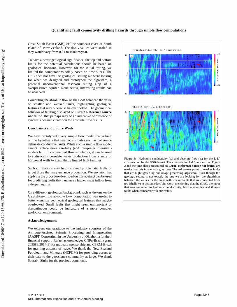
Figure 3: Hydraulic conductivity (a.) and absolute flow (b.) for the L-L’

cross-section for the GSB dataset. The cross-section L-L’ presented on Figure

2 and the time slices presenteed on Error! Reference source not found. are

marked on this image with gray lines.The red arrows point to weaker faults

that are hightlighted by our image processing algorithm. Even though the

geologic setting is not exactly the one we are looking for, the algorirhtm

balanced the values for the areas with weaker faults that are connected from

top (shallow) to bottom (deep).Its worth mentioning that the dLoG, the input

that was converted to hydraulic conductivity, have a smoother and thinner

faults when compared with our results.

© 2017 SEG SEG International Exposition and 87th Annual Meeting

Page 2347

Dow

nloa

ded

10/0

6/17

to 1

29.1

5.66

.178

. Red

istr

ibut

ion

subj

ect t

o SE

G li

cens

e or

cop

yrig

ht; s

ee T

erm

s of

Use

at h

ttp://

libra

ry.s

eg.o

rg/

Quantifying fault connectivity drilling hazards through simple flow computations

Figure 4: Figure 5: Hydraulic conductivity (a. and b.) and absolute flow (c. and d.) for the timseslices on the the GSB dataset. The cross-section L-L’

presented on Figure 2 and the C-C’ cross-section presented on Figure 2 are marked on this image with gray lines. Faults iinside the red circle on panels

a. and c. are stronger and easier to be observed on the absolute flow image. The yellor circle on the panels b. and d. is used to point to an area with possible

presence of syneresis, with the presence of several almost circular faults. This geological feature may be acting as a conductor in difference time slices

and it is highlighted by our image processing algorithm. On the right below corner, inside a greatly faulted area, it is possible to identify an area that was

not faulted or that does not have faults that are connected. (black arrows)

© 2017 SEG SEG International Exposition and 87th Annual Meeting

Page 2348

Dow

nloa

ded

10/0

6/17

to 1

29.1

5.66

.178

. Red

istr

ibut

ion

subj

ect t

o SE

G li

cens

e or

cop

yrig

ht; s

ee T

erm

s of

Use

at h

ttp://

libra

ry.s

eg.o

rg/

EDITED REFERENCES

Note: This reference list is a copyedited version of the reference list submitted by the author. Reference lists for the 2017

SEG Technical Program Expanded Abstracts have been copyedited so that references provided with the online

metadata for each paper will achieve a high degree of linking to cited sources that appear on the Web.

REFERENCES

Gersztenkorn, A., and K. J. Marfurt, 1999, Eigenstructure-based coherence computations as an aid to 3-D

structural and stratigraphic mapping: Geophysics, 64, 1468–1479,

http://dx.doi.org/10.1190/1.1444651.

Harbaugh, A. W., 2005, Chapter 2 – Derivation of the finite-difference equation, MODFLOW-2005. U.S.

Geological Survey, 2.1–2.17.

Höcker, C., and G. Fehmers, 2002, Fast structural interpretation with structure-oriented filtering: The

Leading Edge, 21, 238–243, http://dx.doi.org/10.1190/1.1463775.

Istok, J., 2013, Step 2: Derive the approximating equations, groundwater modeling by the finite element

method: American Geophysical Union, 30–79.

Machado, G., A. Alali, B. Hutchinson, O. Olorunsola, and K. J. Marfurt, 2016, Display and enhancement

of volumetric fault images: Interpretation, 4, SB51–SB61, http://dx.doi.org/10.1190/INT-2015-

0104.

Marfurt, K. J., 2006, Robust estimates of 3D reflector dip and azimuth: Geophysics, 71, no. 4, P29–P40,

http://dx.doi.org/10.1190/1.2213049.

© 2017 SEG SEG International Exposition and 87th Annual Meeting

Page 2349

Dow

nloa

ded

10/0

6/17

to 1

29.1

5.66

.178

. Red

istr

ibut

ion

subj

ect t

o SE

G li

cens

e or

cop

yrig

ht; s

ee T

erm

s of

Use

at h

ttp://

libra

ry.s

eg.o

rg/