Embed Size (px)
Citation preview

Master's Thesis
on the topic
Quanti�er Elimination Testsand Examples
by
Magdalena Forstner
at
Fachbereich Mathematik und Statistik
supervised by
Dr. Panteleimon Eleftheriou
second corrector
Prof. Dr. Salma Kuhlmann
Konstanz, 2017


Acknowledgements
Foremost, I would like to express my sincere gratitude to my supervisor Pantelis Eleftheriou forthe continuous support, for his patience, motivation, and for his most helpful comments. His
guidance helped me in all the time of research and writing of this thesis.
A special thanks goes out to Deirdre Haskell for an interesting and motivating conversation, aswell as for her helpful recommendations on Section 6.1 of this thesis.
Further, I owe my deep gratitude to Chris Miller for his highly valuable answers to myquestions in reference to Section 7.3.
Last but not least, I would like to thank my proofreaders and my loved ones for theirunconditional encouragement. I was continually amazed by their willingness to spend so much
time and e�ort supporting me to �nish this thesis.
Thank you to all of you!


Contents
1 Introduction 1
2 Model Theoretical Background 3
3 Basic Quanti�er Elimination Criteria 11
3.1 First Approach to Quanti�er Elimination . . . . . . . . . . . . . . . . . . . . . . 113.2 Algebraically Closed Fields . . . . . . . . . . . . . . . . . . . . . . . . . . . . . . 153.3 Real Closed Fields . . . . . . . . . . . . . . . . . . . . . . . . . . . . . . . . . . . 17
4 Quanti�er Elimination by Algebraically Prime Models 23
4.1 Algebraically Prime Models and Simple Closedness . . . . . . . . . . . . . . . . . 234.2 Presburger Arithmetic . . . . . . . . . . . . . . . . . . . . . . . . . . . . . . . . . 24
5 Quanti�er Elimination by Types and Saturation 31
5.1 Types and Saturated Models . . . . . . . . . . . . . . . . . . . . . . . . . . . . . 315.2 Di�erentially Closed Fields . . . . . . . . . . . . . . . . . . . . . . . . . . . . . . 35
6 Quanti�er Elimination by Lou van den Dries 43
6.1 Extensions of Partial Embeddings . . . . . . . . . . . . . . . . . . . . . . . . . . . 436.2 The Field of Reals with a Predicate for the Powers of Two . . . . . . . . . . . . . 46
7 Applications 59
7.1 One Geometric Consequence . . . . . . . . . . . . . . . . . . . . . . . . . . . . . . 597.2 Completeness and Decidability . . . . . . . . . . . . . . . . . . . . . . . . . . . . 607.3 De�nable Sets . . . . . . . . . . . . . . . . . . . . . . . . . . . . . . . . . . . . . . 62
Bibliography 65


1 Introduction
In 1927 and 1928 Alfred Tarski was in charge of the seminar on problems in logic at the Uni-versity of Warsaw. He used this seminar to pursue a development of the method of quanti�erelimination. A theory is said to admit quanti�er elimination if every formula is equivalent, in allmodels of the theory, to a formula without any quanti�ers. The term itself is due to Tarski aswell as the following statement about it:
�It seems to us that the elimination of quanti�ers, whenever it is applicable to atheory, provides us with direct and clear insight into both the syntactical structureand the semantical content of that theory�indeed, a more direct and clearer insightthan the modern more powerful methods [. . . ]. � [DoMoTa]
Indeed, quanti�er elimination is a powerful method for a model theoretic investigation ofalgebraic structures. It helps not only in the questions of completeness and decidability but alsofor a better understanding of de�nable sets and the algebraic structure itself, since these studiesare often made rather complicated by quanti�ers.
Under his guidance, Tarski and his students at the Warsaw seminar achieved signi�cant re-sults. Tarski suggested to one of his students�his name was Mojzesz Presburger�to develop anelimination-of-quanti�ers procedure for the additive theory of the integer numbers. The studentsucceded and submitted the result as his thesis for a master's degree. The theory became knownas Presburger Arithmetic and will be subject in this present thesis as well.
Tarksi was able to apply the method of quanti�er elimination to the ordered �eld of realnumbers. In both of these cases, the method yielded a decision algorithm, that is an algorithmwhich decides whether a given sentence is true or false.
There are some equivalent formulations of quanti�er elimination as well as many su�cientconditions that imply quanti�er elimination. Such conditions are called quanti�er eliminationtests. One of the two general aims of this thesis at hand is to prove a few well-known tests andapply them afterwards to some theories. The second aim is to provide a proof of a particularquanti�er elimination test that was introduced in 1985 by Lou van den Dries, but so far, no clearproof has been published. Lou van den Dries is a Dutch mathematician who has successfullybeen applying model theoretical methods to the �eld of real numbers, highly improving theunderstanding of the reals. He also laid the foundation to the concept of o-minimality which hassince become a recognized branch within model theory. Information concerning his work can befound in [UoI]. We will meet the concept of o-minimality again in Theorem 7.10. In most of thetests that we are going to discuss in this thesis, one needs to show the existence of some speci�edelement. The quanti�er elimination test that van den Dries gave in [vdD] di�ers from other tests
1

2 Introduction
as one is rather free in the choice of a particular element. This will become clear once we applythe test to the theory of the �eld of reals with a predicate for the powers of two.
This shall be enough of history and on the signi�cance of quanti�er elimination. Let us givea brief outline of the present thesis.
In the following Chapter 2 we will review some basic notation from mathematical logic andrecall some fundamental model theory which is going to be used in later chapters. At the end ofChapter 2 we will give a formal de�nition of quanti�er elimination.
In Chapter 3 we will provide a simple, yet useful quanti�er elimination test which we will thenapply to the theory of algebraically closed �elds and to the theory of real closed �elds. For thelatter we �rst develop some theory on real closed �elds, whereas for algebraically closed �elds weassume the reader to be already familiar with the topic.
Chapter 4 starts with the notion of algebraically prime models and simple closedness. Thequanti�er elimination test in this chapter follows very quickly. As already promised, we will thendeal with Presburger Arithmetic. All results on this theory given here are due to Presburger,although the speci�c proof of quanti�er elimination given in Section 4.2 is due to van den Dries.
In Chapter 5 we introduce types and saturated models. This is a large realm of model theoryitself. We only provide the theory that we need for another quanti�er elimination test. It followssome background on di�erential �elds. Di�erential algebra is the study of algebraic structuresequipped with a derivation. Model theory has proven quite useful in this area as the de�nition ofdi�erential closure is surprisingly more complex than the analogous notions of algebraic closureor real closure, see [Sac72a]. Once we have set the necessary background, we will prove quanti�erelimination for di�erentially closed �elds.
The main work for this thesis was Chapter 6. This is based on van den Dries' paper [vdD], inwhich the author only stated the quanti�er elimination test without giving a proof. By �ndingsome useful properties of extensions of partial embeddings, we succeded in proving the test. Inthe subsequent section we present a detailed proof of quanti�er elimination for the ordered �eldof real numbers with a predicate for the powers of two.
Finally, in Chapter 7 we conclude this thesis by giving some applications of quanti�er elim-ination. We hereby focus on completeness and decidability as well as on the understanding ofde�nable sets. We will give one geometric consequence, namely the Di�erential Nullstellensatz,which is the analogue of Hilbert's Nullstellensatz for algebraically closed �elds in di�erentialalgebra.

2 Model Theoretical Background
This chapter will give a brief introduction to model theoretic preliminaries which are necessaryfor the following chapters. It pursues the goal of explaining terminology and repeating sometheory that we are going to use several times throughout this thesis. We will assume that thereader is already familiar with basic notions of mathematical logic. We follow the introductorychapters of [Mar02], [Pre86] and [Pre98].
Because in mathematical logic the formal language itself becomes an object of our investigation,one always needs to deal with two languages: On the one hand there is the formal language whichis the object of our study, and on the other hand we have the metalanguage in which we talkabout this formal language. The latter is the mathematical colloquial language. The former,however, the object language, depends on the subject being considered at the time and needs tobe carefully de�ned.
Let I, J and K be arbitrary (possibly empty) index sets and µ : I → N and λ : J → Ntwo functions. For every i ∈ I let fi be a µ(i)-ary function symbol, for every j ∈ J let Rj bea λ(j)-ary relation symbol, and for every k ∈ K let ck be a constant symbol. The functionµ assigns to each i ∈ I the �arity � (i.e. number of arguments) µ(i) of the function symbol fi,whereas the function λ assigns to each j ∈ J the arity λ(j) of the relation symbol Rj . Then,
L = 〈(fi)i∈I ; (Rj)j∈J ; (ck)k∈K〉
is called a language. For a �xed language L, an L-structure
M =(M ; (fMi )i∈I ; (RMj )j∈J ; (cMk )k∈K
)consists of a nonempty set M , called the universe of M, a µ(i)-ary function fMi : Mµ(i) → Mfor each i ∈ I, a λ(j)-ary relation RMj ⊆ Mλ(j), and a �xed element cMk ∈ M for each k ∈ K.The superscript �M � denotes the interpretation of the symbols in M . We will usually namestructures by calligraphic letters and their universe by the corresponding Latin letters, i.e. ifM,N ,A,B are L-strucutres, then we will refer to their underlying universes byM,N,A, and B,respectively.
Additionally to the symbols in a language L we use the following symbols: variable symbolsv, w, v1, v2, . . ., the Boolean connectives ∧,∨, and ¬, the quanti�ers ∃ and ∀, parentheses (,), and the equality symbol = . This list of variables is non-exhaustive, but the context willmake the identi�cation of variables clear. To distinguish the formal object language from themetalanguage, we will usually use = as an equality symbol in the formal language, whereaswe write the usual equality sign = in the metalanguage. If a language contains the functionsymbols +, ·, or < we usually write a+ b, a · b, and a < b instead of +(a, b), ·(a, b), and < (a, b),respectively, for the sake of a better reading. Let for the rest of this introductory chapter L bea �xed language.
3

4 Model Theoretical Background
The set of L-terms is the smallest set which contains all variables and all constant symbols,and for each i ∈ I, it contains fi(t1, . . . , tµ(i)) whenever it contains t1, . . . , tµ(i).We say that φ is an atomic L-formula if it is either of the form t1 = t2 for two L-terms t1
and t2, or it is of the form Rj(t1, . . . , tλ(j)), where Rj is a relation symbol and t1, . . . , tλ(j) areL-terms.
The set of L-formulas is the smallest set consisting of all atomic L-formulas, and that contains¬φ, (φ∧ ψ), (φ∨ ψ), ∃v φ, and ∀v φ for any variable v, whenever it contains φ and ψ. There aretwo abbreviating notations that we will use: φ→ ψ stands for ¬(φ ∨ ψ) and φ↔ ψ is short for(φ → ψ) ∧ (ψ → φ). We will also use the abbreviations
∧ni=1 φi and
∨ni=1 φi for φ1 ∧ . . . ∧ φn
and φ1 ∨ . . . ∨ φn, respectively. The two quanti�ers can be de�ned in terms of each other: ∀v φholds if and only if ¬∃v ¬φ is ful�lled. Hence, in arguments on the complexity of L-formulas itis unnecessary to consider both.
We often write φ(v1, . . . , vn) to make explicit the free variables in φ. Whenever we write�a ∈ A �, we mean that we take a tuple (a1, . . . , an) with components a1, . . . , an from A. Sincein most cases the number n of components does not play an important role and is only meant tosuit the corresponding amount of free variables in some L-formula, we avoid naming the numberand just write �a � instead. Another natural abuse of notation is that, given an L-formulaφ(v1, . . . , vn), a tuple a ∈ A, and some function f : A → B, instead of �φ(f(a1), . . . , f(an)) �we simply write �φ(f(a)) �. And lastly, if a = (a1, . . . , an), then by ca we mean the tuple(ca1 , . . . , can).
If an L-formula has no free variables, we call it an L-sentence. A quanti�er-free L-formula isan L-formula without quanti�ers. An L-formula φ of the form
N∧i=1
ni∨j=1
φij orN∨i=1
ni∧j=1
φij ,
where each φij is an atomic L-formula or the negation of one, is said to be in conjunctive normalform or in disjunctive normal form, respectively. Using the distributive law and De Morgan'slaws, every quanti�er-free L-formula φ can be written in both disjunctive normal form and inconjunctive normal form, with the same free variables.
Next we will de�ne what it means for a formula of a formal language to be satis�ed or tohold in a certain structure and what it means for a structure to be a model of a particularset of sentences, so that we can, for instance, state that a structure in the language of ringsis in fact a ring. For an L-formula φ(v1, . . . , vn) with free variables from v = (v1, . . . , vn) anda = (a1, . . . , an) ∈Mn we de�ne recursivelyM |= φ(a) as follows:
If φ is t1 = t2, thenM |= φ(a), i� tM1 (a) = tM2 (a);
if φ is Rj(t1, . . . tλ(j)), thenM |= φ(a), i� (tM1 (a), . . . , tMλ(j)(a)) ∈ RMj ;
if φ is ¬ψ, thenM |= φ(a), i�M |= ψ(a) does not hold;
if φ is (ψ ∧ θ), thenM |= φ(a), i�M |= ψ(a) andM |= θ(a);
if φ is (ψ ∨ θ), thenM |= φ(a), i�M |= ψ(a) orM |= θ(a);
if φ is ∃w ψ(v, w), thenM |= φ(a), i� there is b ∈M such thatM |= ψ(a, b);
if φ is ∀w ψ(v, w), thenM |= φ(a), i�M |= ψ(a, b) for all b ∈M.

5
An L-theory T is a set of L-sentences, that means a set of L-formulas without any free variables.We say thatM is a model of T and writeM |= T ifM |= φ for all L-sentences φ ∈ T . Moreover,we write T |= φ if for every modelM |= T it holdsM |= φ. An L-theory that satis�es T |= φ orT |= ¬φ for each L-sentence φ is called complete. Occasionally it may be useful to consider thefull theory Th(M) of an L-structure M which consists of all L-sentences φ such that M |= φ.The full theory Th(M) is in fact a complete L-theory.Sometimes it is possible to give a set of L-sentences that form axioms for a theory. We will
call a set of L-sentences Σ an axiom system for an L-theory T if
{φ : φ is an L-sentence and T |= φ} = {φ : φ is an L-sentence and Σ |= φ}.
The L-sentences in Σ are then called axioms. If T already contains each L-sentence φ withT |= φ, we say that T is deductively closed. In this case the L-theory consists exactly of theL-sentences that can be deduced from the axioms and no more. We will later on see a couple ofexamples for such axiom systems.
Of course, as usual in mathematics, we will also consider maps between L-structures. Here wewish that those maps preserve the interpretation of the symbols in the language L. Hence, wede�ne:
2.1 De�nition. LetM and N be two L-structures with universes M and N , respectively. AnL-embedding ι :M→ N is an injective map between the universes ι : M → N which preservesthe interpretation of all function, relation, and constant symbols of L. To be more precise, thismeans:
(i) ι(fM(a)) = fN (ι(a)) for all function symbols f and a ∈M .(ii) a ∈ RM if and only if ι(a) ∈ RN for all relation symbols R and a ∈M .(iii) ι(cM) = cN for all constant symbols c.
If there exists an L-embedding from M into N , we say that M is a substructure of N . Abijective L-embedding is called an L-isomorphism. Sometimes, however, ι(M) is identi�ed withM, hence ifM is a substructure of N we writeM⊆ N .
The following lemma indicates that L-embeddings preserve quanti�er-free formulas that onlyuse parameters from the universe of the substructure. It is therefore known as the SubstructureLemma.
2.2 Lemma (Substructure Lemma). Let M be a substructure of N , a ∈ M , and let φ(v) be aquanti�er-free formula. Then,M |= φ(a) if and only if N |= φ(a).
Proof. For the proof see for example [Mar02, Proposition 1.1.8].
There are maps that preserve quanti�er-free formulas with parameters from a subset of thedomain. They will become very useful later on in Chapter 5.
2.3 De�nition. LetM andN be two L-structures and A a subset ofM , whereM is the universeof M. Then the map η : A → N is called a partial embedding if it preserves all quanti�er-freeformulas. That means, for all quanti�er-free φ(v) and a ∈ A it holds that
M |= φ(a) ⇔ N |= φ(η(a)).

6 Model Theoretical Background
Note that we write a partial embedding η : A→ N technically from a subset into a structure,to point out that the interpretation of the speci�ed formulas is being preserved. However A isonly a subset, thus denoted by a Latin letter.
2.4 De�nition. We say that a collection Σ(v) of L-formulas in n free variables is satis�able ifthere exists an L-structure A with universe A and a tuple a ∈ A, such that A |= φ(a) for everyφ(v) ∈ Σ(v). In particular, an L-theory is called satis�able if it has a model.
By his Completeness Theorem (see [Pre86, Theorem 1.5.2]), Kurt Gödel showed that thesyntactic notion of provability completely coincides with what we semantically call true. TheCompleteness Theorem says that a proposition is true in every model of a theory if and only ifit is provable from the theory. A very important consequence of the Completeness Theorem isthe so called Compactness Theorem. It is the cornerstone of model theory. Until about 50 yearsago, all applications of model theory to algebra were corollaries of the Compactness Theorem,cf. [Sac72a]. Throughout this thesis we will use it several times.
2.5 Theorem (Compactness Theorem). Let T be an L-theory. Then T is satis�able if and onlyif every �nite subset of T is satis�able.
Proof. This follows from Gödel's Completeness Theorem and the fact that any formal proof onlyrequires �nitely many assumptions from the theory T . The proof can for example be found in[Mar02, Theorem 2.1.4].
2.6 De�nition. An L-embedding η :M→N is called an elementary embedding if
M |= φ(a) ⇔ N |= φ(η(a))
for all L-formulas φ(v) and all a ∈M . In this case we say thatM is an elementary substructureof N and writeM� N .
For a subset B ⊆M , we say that η : B → N is a partial elementary map if
M |= φ(b) ⇔ N |= φ(η(b))
for all L-formulas φ(v) and all b ∈ B.Two modelsM,N |= T of an L-theory T are called elementarily equivalent if
M |= φ ⇔ N |= φ
for every L-sentence φ.
Elementary equivalence is strongly related to completeness:
2.7 Proposition. An L-theory T is complete if and only if any two models M,N |= T areelementarily equivalent.
Proof. Let T be a complete L-theory withM |= T andM |= φ for some L-sentence φ. Assumethat T |= ¬φ. ThenM |= ¬φ, a contradiction. By completeness, T |= φ and, hence, N |= φ forany other model N |= T .Suppose otherwise that any two models of T are elementarily equivalent. Let φ be some L-
sentence. IfM |= φ, then for every model N |= T we obtain N |= φ. Hence T |= φ. If on theother handM 6|= φ, thenM |= ¬φ, and therefore, T |= ¬φ.

7
2.8 De�nition. Let M be an L-structure. By LM we denote the language which consists ofthe symbols in L and, additionally, a constant symbol cm for each element m ∈ M . Then Mexpands in a natural way to an LM -structure by interpreting the new symbols in the obviousway cMm = m. The atomic diagram ofM is the set
Diag(M) := {φ(cm) : m ∈M , φ(v) is an atomic L-formula or
the negation of one, andM |= φ(cm)},
where cm stands for (cm1 , . . . , cmn) whenever m = (m1, . . . ,mn). In a similar way we de�ne theelementary diagram ofM to be
Diagel(M) := {φ(cm) : m ∈M , φ(v) is an L-formula andM |= φ(cm)}.
The atomic and the elementary diagram are an e�ective instrument to prove the existence ofL-embeddings. The reason is the next lemma:
2.9 Lemma. LetM be an L-structure and N an LM -structure.
(a) If N |= Diag(M), then, viewing N as an L-structure, there is an L-embedding ofM into N .(b) If N |= Diagel(M), then there is an elementary embedding ofM into N .
Proof. (a) Let j be the interpretation of the constant symbols of LM in N , i.e. j : M → Nwith j(m) = cNm . If m1 and m2 are two distinct elements in M , then ¬cm1 = cm2 is a formula inDiag(M), and hence, since N |= Diag(M), we obtain j(m1) 6= j(m2). Thus, j is an embeddingof sets, i.e. injective. It remains to show that j is an L-embedding:Let f be a function symbol of L, and fM(m1, . . . ,mn) = mn+1. Then f(cm1 , . . . , cmn) = cmn+1
is a formula in Diag(M) and fN (j(m1), . . . , j(mn)) = j(mn+1).
For a relation symbol R of L and m ∈ RM we obtain R(cm1 , . . . , cmn) ∈ Diag(M) and, thus,(j(m1), . . . , j(mn)) ∈ RN . Hence, j is an L-embedding.(b) We will show that if N |= Diagel(M), then the map j from above is elementary. Note
that Diagel(M) is a complete theory: either a sentence is in the set or its negation is. SupposeM |= φ(ca) for some a ∈ M , i.e. φ(ca) ∈ Diagel(M). Since Diagel(M) is complete, this isequivalent to the fact that N |= φ(j(a)). Thus, j is an elementary L-embedding.
For the sake of simplicity, we will often write φ(a) where φ is an L-formula and a ∈ A a tuple,even if a1, . . . , an are not constant symbols in the language, whenever this does not result inambiguity. We then mean φ(ca) after adding a1, . . . , an to the constant symbols and interpretingthem in the natural way, as in LA.In general, the union of models of a certain theory is not even necessarily a well-de�ned
structure. But for elementary extensions we have a very useful property:
2.10 De�nition. We say that (Mi : i ∈ I) is a chain of L-structures, if each Mi is an L-structure andMi ⊆ Mj for every i < j. If additionallyMi � Mj for every i < j, we say that(Mi : i ∈ I) is an elementary chain.
As mentioned before, we will, in particular here, identify a structure with its image underthe embedding. This is, however, not a restriction in any sence, but rather a simpli�cation ofnotation. The unionM =
⋃i∈IMi of a chain of structures is de�ned as follows: The universe
8 Model Theoretical Background
of M is M :=⋃i∈IMi. For a constant c of the language we have cMi = cMj for all i and
j. We set cM := cMi . If f is a function symbol of the language, then fMi(a) = fMj (a) forany a ∈ Mi ∩Mj . Since every a ∈ M is already contained in some Mi, f
M :=⋃i∈I f
Mi iswell-de�ned. For a relation symbol R, we have a ∈ RMi if and only if a ∈ RMj . Thus, we setRM :=
⋃i∈I R
Mi . This implies that eachMi is a substructure ofM.
2.11 Proposition. Let (Mi : i ∈ I) be an elementary chain of L-structures, i.e.Mi �Mj fori < j. Then its limit
M :=⋃i∈IMi
is an elementary extension of eachMi.
Proof. This proposition is due to Alfred Tarski and Robert Vaught and a proof can be found in[Mar02, Proposition 2.3.11].
2.12 De�nition. An L-formula of the form ∀w1∀w2 . . . ∀wn φ(v, w), where φ(v, w) is quanti�er-free, is called a universal L-formula. Similarly, an L-formula of the form ∃w1∃w2 . . . ∃wn φ(v, w)with φ(v, w) quanti�er-free is called existential. For a theory T we denote by T∀ the set of allthe universal L-sentences φ such that T |= φ and call T∀ the universal theory of T .
It requires only a little thought to see that universal statements are preserved downwards ininclusion, whereas existential formulas are preserved upwards in inclusion. The next lemma willbe very useful in section 6.1.
2.13 Lemma. For an L-theory T the following are equivalent:
(i) A |= T∀.(ii) There is a modelM |= T with A ⊆M.
Proof. Universal statements are preserved downwards in inclusion. Therefore we only need todeal with the implication (i) ⇒ (ii): Let A |= T∀. Consider the theory T ′ := T ∪Diag(A) in thelanguage LA. We will show by contradiction that T ′ is satis�able, which implies that there is amodelM |= T ′, i.e. M |= T andM |= Diag(A). With the latter we obtain by Lemma 2.9 anL-embedding of A intoM.
Hence, let us suppose that T ′ is not satis�able. Then, by the Compactness Theorem, alreadysome �nite subset ∆ ⊆ T ′ is not satis�able. By forming conjunctions we may assume that thepart of ∆ coming from Diag(A) consists only of one formula φ(a) for some a ∈ A, where φ(a)is a conjunction of atomic formulas and the negation of atomic formulas. Thus, we will assumethat T ∪ {φ(a)} is not satis�able. In particular, φ(a) is quanti�er-free and, as Diag(A) |= φ(a),we obtain A |= φ(a).
On the other hand, viewing T as an La -theory, and because T ∪ {φ(a)} is not satis�able, weobtain T |= ¬φ(a). We will show that this implies T |= ∀v ¬φ(v): Let C be an L-structurewith C |= T . Let n be the number of components in a and c1, . . . , cn ∈ C be any tuple. Let C′be the La -structure which expands C by the constant symbols a1, . . . , an, that we interpret asc1, . . . , cn, respectively. Then C′ |= T and, hence C′ |= φ(c). As this follows for any tuple in C,we get C |= ∀v ¬φ(v) and, thus, T |= ∀v ¬φ(v) as claimed.
Since T∀ consists exactly of the universal formulas which hold in all models of T , we obtainT∀ |= ∀x ¬φ(x). Hence, also A |= ∀x ¬φ(x), which is a contradiction because we also hadA |= φ(a).

9
Therefore, as desired, T ′ is indeed satis�able.
After this short introduction to mathematical logic and model theory, we can �nally give aproper de�nition of quanti�er elimination and hereby start discussing the main purposes of thisthesis.
2.14 De�nition. An L-theory T is said to admit elimination of quanti�ers if for any L-formulaφ(v) there is a quanti�er-free L-formula ψ(v) such that the following holds:
T |= ∀v (φ(v)↔ ψ(v)).
A weaker concept than quanti�er elimination is the property of model completeness. Thefollowing theorem is called Robinson's Test. We call an L-theory T model complete if one of thefollowing equivalent conditions holds:
2.15 Theorem (Robinson's Test). For an L-theory T the following are equivalent:
(i) All L-embeddings of models of T are elementary.(ii) Let M,N |= T be two models, where M ⊆ N . For every existential L-formula φ(v) and
a ∈M with N |= φ(a) it followsM |= φ(a).(iii) For every L-formula φ(v) there exists a universal L-formula ψ(v) such that it holds
T |= ∀v (φ(v)↔ ψ(v)).
Proof. See [Pre98, Lemma 3.3.1 and Theorem 3.3.3].
By condition (iii) of Robinson's Test, a theory is obviously model complete whenever it admitsquanti�er elimination.
A language L without constant symbols does not produce any quanti�er-free L-sentences.Hence, to make sense of the expression �quanti�er-free L-sentence �, we will always assume thatour languages contain at least one constant symbol.
It is important to remark that quanti�er elimination is a matter of language. We will see thatsome theories only admit quanti�er elimination after adding some predicates to the language.
Having de�ned what it means for an L-theory to eliminate quanti�ers, we may now end thisintroductory chapter and start the next one with the �rst quanti�er elimination test.


3 Basic Quanti�er Elimination Criteria
3.1 First Approach to Quanti�er Elimination
This section is based on [Mar02, Section 3.1]. The proofs, however, will be presented in more de-tail than in the source. We will prove two lemmas in order to obtain a �rst quanti�er eliminationtest from the combination of both.
3.1 Lemma. Let L be a language that contains at least one constant symbol c, T an L-theory,and φ(v) an L-formula. Then the following are equivalent:
(i) If M and N are models of T , and A is a common substructure, then for any tuple a ∈ Awe haveM |= φ(a) if and only if N |= φ(a).
(ii) There is a quanti�er-free L-formula ψ(v) such that T |= ∀v (φ(v)↔ ψ(v)).
Proof. (i) ⇒ (ii): If T |= ∀v φ(v), then T |= ∀v (φ(v) ↔ c = c) and we have found thecorresponding quanti�er-free formula: c = c. If, on the other hand, T |= ∀v ¬φ(v), then we haveT |= ∀v (φ(v)↔ ¬c = c) and we are also done. So we may assume that we are in the third casewhere none of the above is true, i.e., there exists a modelM1 of T that does not model ∀v φ(v)and there is a modelM2 of T that does not model ∀v ¬φ(v). This means thatM1 |= ∃v ¬φ(v)andM2 |= ∃v φ(v), and, thus, both T ∪ {¬φ(v)} and T ∪ {φ(v)} are satis�able.De�ne the set Γ(v) = {ψ(v) : ψ is quanti�er-free and T |= ∀v (φ(v)→ ψ(v))}. Let c1, . . . , cm
be new constant symbols. We will view T now as an Lc -theory where Lc is the language Lextended by the constant symbols c1, . . . , cm. We will show that T ∪ Γ(c) |= φ(c).
Assume that this is not the case. Then there is a modelM |= T ∪Γ(c)∪{¬φ(c)}. Let A be thesubstructure ofM generated by c, i.e. the smallest substructure ofM that contains c1, . . . , cm.
Let Σ = T ∪Diag(A) ∪ {φ(c)}. Let us assume that Σ were not satis�able. So, for any modelB |= T ∪ Diag(A), one obtains B |= ¬φ(c). Thus T ∪ Diag(A) |= ¬φ(c). By the CompactnessTheorem there are �nitely many ψ1(c), . . . , ψn(c) ∈ Diag(A) which are quanti�er-free L-formulassuch that
T ∪ {ψ1(c), . . . , ψn(c)} |= ¬φ(c).
Let C |= T , and suppose that C |= {ψ1(c), . . . , ψn(c)}, i.e. C |= ψ1(c) ∧ . . . ∧ ψn(c). Then,C |= ¬φ(c). Hence
T |=n∧i=1
ψi(c)→ ¬φ(c). (3.1)
11

12 Basic Quanti�er Elimination Criteria
Viewing T as an L-theory again, this yields
T |= ∀v
(n∧i=1
ψi(v)→ ¬φ(v)
)
as in Lemma 2.13: Let D be an L-structure such that D |= T . Let d1, . . . , dm ∈ D be any tupleof the size of a. Let D′ be the Lc -structure which expands D by the constant symbols c1, . . . , cm,that we interpret as d1, . . . , dm, respectively. Then, D′ |= T and, by (3.1), we obtain
D′ |=n∧i=1
ψi(d)→ ¬φ(d).
Since this does not depend on the choice of the tuple d, we obtain
D |= ∀v
(n∧i=1
ψi(v)→ ¬φ(v)
)and thus T |= ∀v
(n∧i=1
ψi(v)→ ¬φ(v)
),
as claimed. Forming the contrapositive we obtain
T |= ∀v
(φ(v)→
n∨i=1
¬ψi(v)
).
By the de�nition of Γ, this meansn∨i=1
¬ψi(v) ∈ Γ(v).
SinceM |= Γ(c) and because ¬ψi(c) is quanti�er-free, this also yields
A |=n∨i=1
¬ψi(c)
by Lemma 2.2, since A is the substructure ofM which is generated by c. This is a contradictionto ψ1(c), . . . , ψn(c) ∈ Diag(A) and A |= Diag(A).
Thus, we may conclude that our assumption �Σ is not satis�able � was wrong and Σ is indeedsatis�able. Let N |= Σ. Then N |= φ(c), and N |= Diag(A). By Lemma 2.9, this means thatthere is an L-embedding from A into N , i.e. A is a substructure of N . Recall thatM is a modelof T ∪ Γ(c) ∪ {¬φ(c)}, so M |= ¬φ(c). Since both M and N are models of T , we may apply(ii) and conclude that also N |= ¬φ(c). This is a contradiction. Hence, also the assumption thatT ∪ Γ(c) 6|= φ(c) was wrong and, thus, we obtain T ∪ Γ(c) |= φ(c).
By the Compactness Theorem, this means that there are �nitely many quanti�er-free L-formulas χ1(c), . . . , χm(c) ∈ Γ(c) such that
T ∪ {χ1(c), . . . , χm(c)} |= φ(c).
Again by the same argumentation as before we may conclude
T |= ∀v
(m∧i=1
χi(v)→ φ(v)
).

First Approach to Quanti�er Elimination 13
Since χ1, . . . , χm ∈ Γ, this yields
T |= ∀v
(m∧i=1
χi(v)↔ φ(v)
),
where∧ni=1 χi(v) is quanti�er-free. Thus, we have completed the �rst�and the more interesting�
implication of the proof.
(ii) ⇒ (i): Suppose that T |= ∀v (φ(v) ↔ ψ(v)) for a quanti�er-free formula ψ(v). Let Mand N be two models of T , A a common substructure ofM and N , and a ∈ A. By Lemma 2.2,quanti�er-free formulas are preserved under substructure and extension. Hence, we obtain
M |= φ(a) ⇔ M |= ψ(a) sinceM |= T , by assumption of (ii)
⇔ A |= ψ(a) since A ⊆M⇔ N |= ψ(a) since A ⊆ N⇔ N |= φ(a) since N |= T , by assumption of (ii).
The following lemma states that if one existential quanti�er can be eliminated at a time, wealready obtain quanti�er elimination.
3.2 Lemma. Let T be an L-theory. Suppose that for every quanti�er-free L-formula θ(w, v)there is a quanti�er-free formula ψ(v) such that T |= ∀v ((∃w θ(w, v)) ↔ ψ(v)). Then T hasquanti�er elimination.
Proof. Let φ(v) be any L-formula. We want to show that there is some quanti�er-free L-formulaψ(v) such that T |= ∀v (φ(v) ↔ ψ(v)). We will prove this by induction on the complexity ofφ(v).
If φ(v) is quanti�er-free, we are already done. So, as induction hypothesis, suppose thatfor φ1(v) and φ2(v) there already exist quanti�er-free L-formulas ψ1(v) and ψ2(v) such thatT |= ∀v (φ1(v)↔ ψ1(v)) and T |= ∀v (φ2(v)↔ ψ2(v)). In the case that φ(v) = ¬φ1(v), we haveT |= ∀v (φ(v)↔ ¬ψ1(v)). And if φ(v) = φ1(v) ∧ φ2(v), then T |= ∀v (φ(v)↔ (ψ1(v) ∧ ψ2(v))).In either case, φ is equivalent to a quanti�er-free formula.
Now suppose φ(v) = ∃x φ1(x, v). By induction hypothesis there is a quanti�er-free L-formulaψ1(x, v) such that T |= ∀v∀x (φ1(x, v)↔ ψ1(x, v)). Then we obtain
T |= ∀v (∃x φ1(x, v)↔ ∃x ψ1(x, v)) (3.2)
as follows: Let M |= T and a ∈ M . Suppose that M |= φ1(b, a) for some b ∈ M . Then sinceM |= ∀v∀x (φ1(x, v) ↔ ψ1(x, v)), also M |= ψ1(b, a). So, M |= ∃x φ1(x, a) → ∃x ψ1(x, a).Similarly we obtain the other implication. Hence,M |= ∃x φ1(x, a) ↔ ∃x ψ1(x, a). This shows(3.2) as claimed.
Now by assumption there is ψ(v) quanti�er-free such that
T |= ∀v (∃x ψ1(x, v)↔ ψ(v)). (3.3)
Hence from (3.2) and (3.3) we obtain
T |= ∀v (∃x φ1(x, v)↔ ψ(v)),
which was to be shown.

14 Basic Quanti�er Elimination Criteria
The previous two lemmas set a decent foundation and both of them combined, they yield asimple, yet useful, quanti�er elimination test.
Algebraically Closed Fields 15
3.3 Theorem. Let T be an L-theory. The following are equivalent:
(i) Let M,N |= T , A a common substructure of M and N , φ(w, v) a quanti�er-free L-formula, and a ∈ A. IfM |= ∃x φ(x, a), then N |= ∃x φ(x, a).
(ii) T has quanti�er elimination.
Proof. (i) ⇒ (ii): Considering Lemma 3.2, it su�ces to show that for an L-formula ∃x φ(x, v),where φ(x, v) is quanti�er-free, there is a quanti�er-free L-formula ψ(v) such that it holdsT |= ∀v (∃x φ(x, v) ↔ ψ(v)). So, suppose that there are two models M,N |= T , a com-mon substructure A of M and N , and a tuple a ∈ A. Suppose further that M |= ∃x φ(x, a).Then, by our assumption, it follows that N |= ∃x φ(x, a). SinceM and N are interchangeable,this is an equivalence. Therefore, we may apply Lemma 3.1 and conclude that T has quanti�erelimination.
(ii) ⇒ (i): Suppose that T eliminates quanti�ers. LetM,N , and A be de�ned as above. Letφ(w, v) be quanti�er-free. By quanti�er elimination there exists a quanti�er-free formula ψ(v),such that T |= ∀v (∃x φ(x, v)↔ ψ(v)). Let a ∈ A. We obtain
M |= ∃x φ(x, a) ⇔ M |= ψ(a) becauseM |= T⇔ A |= ψ(a) by Lemma 2.2
⇔ N |= ψ(a) again by Lemma 2.2
⇔ N |= ∃x φ(x, a) because N |= T .
In the following two sections we will apply this test to two well-known examples for theoriesthat allow quanti�er elimination.
3.2 Algebraically Closed Fields
We will assume that the reader already knows enough about algebraically closed �elds to followthe proof of quanti�er elimination for the theory of algebraically closed �elds. Nevertheless, wewill prove one statement that will be the crucial point at the very end of the proof.
3.4 Lemma. Every algebraically closed �eld has in�nitely many elements.
Proof. Assume that there was a �nite algebraically closed �eld K = {a1, a2, . . . , an} with nelements. Let f ∈ K[X] be the polynomial
f =n∏i=1
(X − ai),
which vanishes on every element of K. Now consider the polynomial g = f + 1. One can easilysee that g does not have any root in K, which is a contradiction to the fact that K is algebraicallyclosed.

16 Basic Quanti�er Elimination Criteria
3.5 De�nition. Let L be the language of rings 〈+ ,− , · ; 0 , 1〉, where �− � will throughout thethesis always denote the binary relation of substraction. The theory ACF of algebraically closed�elds is axiomatized by the following axioms:
� the �eld axioms:
K1: ¬0 = 1K2: ∀x∀y∀z (x+ (y + z) = (x+ y) + z)K3: ∀x (x+ 0 = x)K4: ∀x (x+ (−x) = 0)K5: ∀x∀y∀z (x · (y · z) = (x · y) · z)K6: ∀x (x · 1 = x)K7: ∀x∃y (x = 0 ∨ x · y = 1)K8: ∀x∀y (x · y = y · x)K9: ∀x∀y∀z ((x+ y) · z = (x · z) + (y · z))
� every monic polynomial has a zero:
AKn: ∀x0∀x1 . . . ∀xn∃y yn+1 + xnyn + . . .+ x1y + x0 = 0 for each n ∈ N.
In axiom AKn we used a simpli�ed notation: As it is generally kept in mathematics, weusually relinquish the function symbol · of multiplication, and we write xn instead of x · . . . · x︸ ︷︷ ︸
n times
.
We will now show by using Theorem 3.3 that ACF eliminates quanti�ers.
3.6 Theorem. The theory ACF of algebraically closed �elds admits quanti�er elimination.
Proof. Let F1,F2 |= ACF, A a common substructure of F1 and F2. Then A is a model of theuniversal theory ACF∀. Let us investigate what that means for A: Since in the language L, thereis + and ·, it will be closed under addition and multiplication, and − guarantees the existence ofadditive inverse elements. Hence, A is a ring. Since it is a subring of the �elds F1 and F2, it iseven an integral domain. This allows us to form the �eld of fractions, Quot(A). Since Quot(A)is the smallest �eld which contains A, we obtain Quot(A) ⊆ F1,F2. Let F be the algebraicclosure of Quot(A). Since F1 and F2 are two algebraically closed �elds, this directly yields thatF ⊆ F1,F2.
Let φ(x, y) be a quanti�er-free L-formula and a ∈ A. Assume that F1 |= ∃x φ(x, a). We wishto show F2 |= ∃x φ(x, a) in order to apply Theorem 3.3. Without loss of generality, we canassume that
φ(x, a) =N∨i=1
ni∧j=1
φij(x, a)
︸ ︷︷ ︸
=:φi(x,a)
,
where each φij(x, a) is of the form pij(x) = 0 or qij(x) 6= 0 for polynomials pij and qij in thevariable X whose coe�cients are themselves polynomials in the constants a occurring in φ withinteger coe�cients. Note that thus pij(X), qij(X) ∈ A[X]. Further note that the cases m = 0and ni = 0 are not excluded.
Since ∃x φ(x, a) is logically equivalent to ∃x φ1(x, a) ∨ . . . ∨ ∃x φm(x, a) and because of ourassumption F1 |= ∃x φ(x, a), we may as well assume that F1 |= ∃x φ1(x, a). If we show that
Real Closed Fields 17
F2 |= ∃x φ1(x, a), then it follows naturally that F1 |= ∃x φ(x, a). We distinguish the followingtwo cases:
Case 1: Suppose that at least one of the p1,j is not the zero polynomial in A[X], say p1,1 6= 0.Then there is b ∈ F such that F1 |= φ1(b, a), in particular p1,1(b) = 0. But any root of p1,1 is
already contained in F . Thus, b ∈ F and hence, F |= ∃x φ1(x, a). This yields F |= ∃x φ(x, a),and therefore F2 |= ∃x φ(x, a).
Case 2: If, on the other hand, all terms p1,j are equal to the zero polynomial or if there is no
term p1,j(x) = 0 in φ1(x, a), then it su�ces to �nd an element b ∈ F that di�ers from all the zerosof the polynomials q1,j . One such b does, indeed, exist, since there are only �nitely many zeros
of the q1,j and, as an algebraically closed �eld, by Theorem 3.4, F has in�nitely many elements.
Therefore we obtain F |= ∃x φ1(x, a), i.e. F |= ∃x φ(x, a) and, hence, also F2 |= ∃x φ(x, a).
3.3 Real Closed Fields
Tarski gave an explicit algorithm for eliminating quanti�ers in the theory of real closed �elds.This is the theory of the �eld of the reals, which is equipped with a natural order.
In this section we will review some of the necessary results on real closed �elds which we willlater on use to prove quanti�er elimination. We start with some basic notion:
3.7 De�nition. An ordering on a �eld K is a total order relation ≤ such that for all a, b, c ∈ Kit holds that
a ≤ b ⇒ a+ c ≤ b+ c and
a ≤ b ∧ c ≥ 0 ⇒ ac ≤ bc.
An ordered �eld (K,≤) is a �eld K, equipped with an ordering ≤. If the order is clear, however,we just write K.
3.8 De�nition. We say that a �eld K is real if it has an ordering ≤. For an ordered �eld (K,≤),the subset P = {x ∈ K : x ≥ 0} is called the positive cone of (K,≤).
Equivalently we could say that a �eld K is called real, if −1 cannot be written as a sum ofsquares in K. We are familiar with Q and R as real �elds with their natural orderings. But alsothe �eld of rational functions in one variable over Q is real. In fact, if R is any ordered �eld,then R(t), the �eld of rational functions in one variable over R, also admits an ordering.
3.9 De�nition. An ordered �eld R is real closed if R is real and does not admit any properalgebraic extension which is real itself and whose ordering extends the ordering on R.
Usually real closed �elds are denoted by the letter R. We will stick to this convention. Thereare many equivalent formulations of a de�nition for real closed �elds:
3.10 Lemma. Let R be a �eld. Then the following are equivalent:
(i) R is real closed.(ii) There is an ordering on R which cannot be extended to any proper algebraic extension of
R.

18 Basic Quanti�er Elimination Criteria
(iii) There is an ordering of R whose positive cone is R2 = {a2 : a ∈ R}, and every polynomialof R[X] of odd degree has a root in R.
(iv) R is real, for every a ∈ R, either a or −a is a square in R, and every polynomial of R[X]of odd degree has a root in R.
Proof. See [KnSc, Section 1.5, Satz 1 and Bemerkung] for a proof.
3.11 Lemma. If R is a real closed �eld, then R(√−1) is algebraically closed.
Proof. A proof, which is due to Carl Friedrich Gauÿ, can be found in [KnSc, Section 1.5, Theo-rem 2].
Lemma 3.10(iii) immediately yields that the ordered �eld of real numbers R is real closed.From Lemma 3.11 we deduce the Intermediate Value Theorem for real closed �elds:
3.12 Theorem (Intermediate Value Theorem). Let R be a real closed �eld, f ∈ R[t], a, b ∈ Rwith a < b. If f(a) · f(b) < 0, then the number of zeros in the interval ]a, b[ is odd. In particular,there exists x ∈ ]a, b[ such that f(x) = 0.
Proof. Let a1 ≤ . . . ≤ ar be the roots of f . By Lemma 3.11, the degree of the �eld extension[R(√−1) : R] is 2, i.e. the irreducible factors of f are either linear or quadratic polynomials.
Hence, f is of the form f = c · (t− a1) · . . . · (t− ar) · p1(t) · . . . · ps(t), where c is a unit in R andp1, . . . , ps are irreducible monic quadratic polynomials. Since the pk only take positive values,we obtain
−1 = signf(a)
f(b)=
r∏i=1
signa− aib− ai
.
Thus, the number of ai with a < ai < b is odd.
3.13 De�nition. A real closure of an ordered �eld K is a real closed �eld R ⊇ K, such that Ris algebraic over K and the order on R extends the order on K.
3.14 Lemma. Every ordered �eld K has a real closure. If R and R′ are two real closures of K,there is one unique order-preserving K-isomorphism between R and R′. Thus, we speak of thereal closure of K.
Proof. We only sketch the proof of the �rst statement: For an ordered �eld (K,≤) one needs toapply Zorn's lemma to the set
L = {L ⊇ K : L is an ordered �eld, L is algebraic over K, and extends the order on K}
and verify that the maximal element of L is indeed real closed. The proof of the second partneeds some more machinery. The whole proof of the lemma can be found in detail, for example,in [BoCoRo, Theorem 1.3.2].
3.15 Lemma. Let R be a real closed �eld, K ⊆ R a sub�eld, and K the relative algebraic closureof K in R, i.e. K = {x ∈ R : x is algebraic over K}. Then K is real closed.

Real Closed Fields 19
Proof. We will verify version (iv) of Lemma 3.10. Since K is a sub�eld of R, we can restrictthe ordering on R to K. Hence, K is real. Now let a ∈ K. We may assume that a ≥ 0,as otherwise we can consider −a instead. Since R is real closed, the quadratic polynomialX2 − a ∈ K[X] ⊆ R[X] has a root b ∈ R. As b is algebraic over K, it is also algebraic over K,and thus contained in K. A similar argument can be applied to any polynomial in K[X] of odddegree to show that it has a root in K.
After giving an axiomatization of the theory of real closed �elds, we are ready to prove quan-ti�er elimination.

20 Basic Quanti�er Elimination Criteria
3.16 De�nition. Let L be the language of ordered rings 〈+ ,− , · ;< ; 0 , 1〉. The theory of RCFof real closed �elds is axiomatized by the following axiom system:
� the �eld axioms K1 to K9,
� the order axioms:
O1: ∀x ¬x < xO2: ∀x∀y∀z ((x < y ∧ y < z)→ x < z)O3: ∀x∀y (x < y ∨ x = y ∨ y < x)O4: ∀x∀y∀z (x < y → x+ z < y + z)O5: ∀x∀y ((0 < x ∧ 0 < y)→ 0 < x · y)
� positive elements are squares:
RK1: ∀x (0 < x → ∃y x = y2)
� polynomials of odd degree have zeros: For each n ∈ N we have:
RK2n: ∀x0∀x1 . . . ∀x2n ∃y y2n+1 + x2ny2n + x2n−1y
2n−1 + . . .+ x1y + x0 = 0.
Note that in the language of ordered rings we use < for the order relation while in the de�nitionof ordered �elds it is common to use ≤. This does not cause any di�culties though, as the twosymbols are interde�nable.
Using the criterion of Theorem 3.3 again, we will now show quanti�er elimination for realclosed �elds. The proof is very similar to the one of Theorem 3.6.
3.17 Theorem. The theory of real closed �elds RCF admits quanti�er elimination.
Proof. Let B1,B2 |= RCF and A a common substructure of both B1 and B2. Let φ(x, y) be aquanti�er-free L-formula and a ∈ A such that B1 |= ∃x φ(x, a). By Theorem 3.3 we need toshow that this implies B2 |= ∃x φ(x, a).
Without loss of generality, φ(x, y) only uses the logical operators ∧,∨, and ¬ such that ¬only occurs in front of atomic formulas. Atomic formulas have the form 0 = p(x) or 0 < q(x),where p and q are polynomials in the variable X whose coe�cients are again polynomials inthe constants a1, . . . , an with integer coe�cients. Moreover, we can replace ¬p(x) = 0 by theexpression (0 < p(x) ∨ 0 < −p(x)) and ¬0 < q(x) by (0 = q(x) ∨ 0 < −q(x)). Therefore, wecan assume that φ(x, a) only uses ∧ and ∨ as logical connectives. So we have
φ(x, a) =
N∨i=1
ni∧j=1
φij(x, a)
︸ ︷︷ ︸
=:φi(x,a)
,
where φij(x, a) is of the form p(x) = 0 or 0 < q(x). The formula ∃x φ(x, a) is logically equivalentto ∃x φ1(x, a) ∨ . . . ∨ ∃x φm(x, a). Because B1 |= ∃x φ(x, a), without loss of generality supposethat B1 |= ∃x φ1(x, a). We now show that B2 |= ∃x φ1(x, a), since this implies B2 |= ∃x φ(x, a).
We know that φ1(x, a) is of the form
s∧k=1
qk(x) > 0 ∧n1∧
k=s+1
pk(x) = 0.

Real Closed Fields 21
In ordered �elds, it holds that ps+1(x) = 0, . . . , pn1(x) = 0 if and only if the sum of all squaresvanishes, i.e.
∑n1k=s+1 pk(x)2 = 0. Therefore, φ1(x, a) even has the form
s∧k=1
qk(x) > 0 ∧ p(x) = 0,
where p(x) :=∑n1
k=s+1 pk(x)2. That means
B1 |= ∃x
(s∧
k=1
qk(x) > 0 ∧ p(x) = 0
).
Since A is a substructure, it is, again, a subring of a �eld, hence, an integral domain. LetQuot(A) be its �eld of fractions and let R1 and R2 be the relative algebraic closures of Quot(A)in B1 and B2, respectively. By Lemma 3.15, R1 and R2 are also real closed, i.e. R1 |= RCF andR2 |= RCF. By Lemma 3.14, R1 and R2 are isomorphic, so we will identify them with eachother and just write R instead. Because B1 |= ∃x φ1(x, a), there exists α ∈ B1 such that
B1 |=s∧
k=1
qk(α) > 0 ∧ p(α) = 0.
We will show that there exists b ∈ R such that
R |=s∧
k=1
qk(b) > 0 ∧ p(b) = 0,
because in this case it follows R |= ∃x φ1(x, a) and therefore also B2 |= ∃x φ1(x, a), sinceb ∈ R ⊆ B2. We distinguish the following two cases:
Case 1: p is not the zero-polynomial in R[X]. Since R is relatively algebraically closed in B1,it holds that α ∈ R, so α ∈ B2 and we are done.
Case 2: p is the zero-polynomial in R[X] or s = n1 which means that there is no conditionp = 0 in φ1. If the q1, . . . , qs do not have any zeros in R, then they do not change sign and itholds for all b ∈ R that qk(b) > 0. Otherwise, let β1 < . . . < βt be the zeros of q1, . . . , qs in R.We have one of the following situations:
(1) α < β1,(2) βi < α < βi+1 for some i ∈ {1, . . . , t− 1},(3) βt < α.
Note that α is not a zero of any qk. In situation (1) choose b = β1 − 1 ∈ R. In (2) takeb = 1
2(βi + βi+1) ∈ R. And in the last situation (3), b = βt + 1 ∈ R will do.
It follows from the Intermediate Value Theorem 3.12 for B1 that qk(b) > 0 for all k = 1, . . . , s.If not, there would be another zero between b and one βi in R, not included in {β1, . . . , βt}, acontradiction. Hence, b satis�es ∃x φ1(x, a) and this yields B2 |= ∃x φ(x, a).

4 Quanti�er Elimination by
Algebraically Prime Models
4.1 Algebraically Prime Models and Simple Closedness
For this section we use the terminology that David Marker uses in [Mar02]. The notion ofalgebraically prime models and simple closedness is not common otherwise in the literature. Forthe following quanti�er elimination test there is nothing really new happening in this section. Itwill, however, be handy to prove quanti�er elimination of Presburger Arithmetic.
4.1 De�nition. A theory T has algebraically prime models if for any A |= T∀ there is A |= Tand an L-embedding i : A → A such that for all N |= T and L-embeddings j : A → N there isan L-embedding h : A → N such that j = h ◦ i.
4.2 De�nition. Let M,N |= T , where M ⊆ N . We call M simply closed in N if for anyquanti�er-free formula φ(v, w) and any a ∈M , if N |= ∃x φ(a, x) thenM |= ∃x φ(a, x).
The following quanti�er elimination test can be found in [Mar02, Corollary 3.1.12] and theproof is a modi�cation of the proof of [Mar02, Theorem 3.1.9].
4.3 Theorem. Suppose that T is an L-theory such that
(i) T has algebraically prime models,(ii) wheneverM⊆ N are models of T ,M is simply closed in N .
Then T has quanti�er elimination.
Proof. We are going to use the quanti�er elimination test from Theorem 3.3: Let T be an L-theory as above. Let φ(v, x) be a quanti�er-free formula,M,N |= T , A a common substructureofM and N , a ∈ A, b ∈ M such thatM |= φ(a, b). We want to show that there is c ∈ N suchthat N |= φ(a, c). For simplicity reasons we suppose without loss of generality that A is notonly a substructure ofM and N but also properly contained in both such that the substructureembeddings are the identity map.
By Lemma 2.13 we know that A |= T∀. Since T has algebraically prime models, there isA |= T and an L-embedding i : A → A such that for all B |= T and L-embeddings j : A → Bthere is an L-embedding h : A → B such that j = h ◦ i. In particular, by setting B = N , weobtain an L-embedding β : A → N such that β ◦ i = id. Similarly by setting B = M we getα : A →M such that α ◦ i = id.
As A |= T ,M |= T and A ⊆ M, A is simply closed inM. Moreover, we have i(a) ∈ A andα(i(a)) = a ∈ M . By assumption we have M |= ∃x φ(a, x). Hence, by simple closedness, it
23

24 Quanti�er Elimination by Algebraically Prime Models
follows A |= ∃x φ(i(a), x). Now by applying β this yields A |= ∃x φ(a, x). Thus, we have shownthat there exists an element, say c ∈ N , such that N |= φ(a, c).
So, by Theorem 3.3, T has quanti�er elimination.
4.2 Presburger Arithmetic
Presburger Arithmetic is formally de�ned as the theory of the natural numbers with addition.It is due to Mojzesz Presburger and, therefore, named after him Presburger Arithmetic. As itcompletely omits multiplication, it is much weaker than Peano Arithmetic, which includes bothaddition and multiplication. It cannot de�ne terms such as prime numbers or divisibility by avariable, for instance. But, unlike Peano Arithmetic, it is a complete and decidable theory. Wewill come back to this concept in Chapter 7.
Let L be the language 〈+ ,− ;< ; 0 , 1〉. Roughly speaking, Presburger Arithmetic is the theoryof the ordered group of integers. It does not have quanti�er elimination in the language L. Theproblem is formulas of the following type
φ(x) = ∃y (x = y + . . .+ y︸ ︷︷ ︸n times
),
which asserts that x is divisible by n. Once having de�ned properly what Pr, the theory ofPresburger Arithmetic, is, we will show that the above formula is not equivalent to a quanti�er-free L-formula.If we add predicates for being divisible by some integer n to the language L, however, quanti�er
elimination is admitted in the extended language. Thus, let Pn be a unary predicate which weinterpret as �the element is divisible by n � and let L∗ = L∪{Pn : n = 2, 3, . . .} be the extendedlanguage. Since we only add predicates for sets that one can already de�ne in L, we do notchange the de�nable sets by extending the language.
There is another axiomatization of Pr than the one that we will give in the following, see forinstance [Poi, page 115]. We follow [Mar02, page 82].
4.4 De�nition. The L∗-theory Pr for Presburger Arithmetic is axiomatized by the followingaxiom system:
� axioms for Abelian groups,
AG1: ∀x (0 + x = x+ 0 = x)AG2: ∀x∀y∀z (x+ (y + z) = (x+ y) + z)AG3: ∀x (x− x = 0)AG4: ∀x∀y (x+ y = y + x)
� the order axioms O1, O2, O3 and O4
� and additionally:
P1: 0 < 1P2: ∀x (x ≤ 0 ∨ x ≥ 1)
P3n: ∀x(Pn(x)↔ ∃y (x = y + . . .+ y︸ ︷︷ ︸
n times
))for n = 2, 3, . . .

Presburger Arithmetic 25
P4n: ∀x(n−1∨i=0
(Pn(x+ 1 + . . .+ 1︸ ︷︷ ︸
i times
) ∧∧j 6=i¬Pn(x+ 1 + . . .+ 1︸ ︷︷ ︸
j times
)))
for n = 2, 3, . . .
Without adding the predicates Pn to the language, the above formula φ(x) is not equivalentin the theory to a quanti�er-free formula. Let Pr′ be the L-theory which is de�ned by the sameaxioms as Pr, except for P3n and P4n, since they require the predicates Pn, which are not in thelanguage L. The following proposition shows that the L-theory Pr′ does not admit eliminationof quanti�ers in L:
4.5 Proposition. In Pr′, the formula ∃x (y = x + x) is not equivalent to a quanti�er-freeL-formula.
Proof. Consider the group G := Z[ω], which is generated by the integers and an in�nite elementω, and H := Z[ω/2], both equipped with the usual addition. Then G ⊆ H. Note that in H, thereis an element x such that ω = x+ x, namely ω/2. In G, however, there is no such element.
Now let us suppose that there is a quanti�er-free L-formula ψ(v) such that it holdsPr |= ∀y (∃x y = x + x ↔ ψ(y)). As one can quickly check with the axiomatization ofPresburger Arithmetic, G and H are both models of Pr. Hence, H |= ∀y (∃x y = x+ x↔ ψ(y))and G |= ∀y (∃x y = x+ x↔ ψ(y)). Now we are in one of the following two cases:
Case 1: H |= ψ(ω). Equivalently one has H |= ∃x ω = x+ x. As G is a substructure of H andψ(ω) is quanti�er-free, we also obtain G |= ψ(ω), which holds if and only if G |= ∃x ω = x + x.But, as we have noted in the beginning, ∃x ω = x + x holds in H but not in G. Hence, we arein the second case:
Case 2: H |= ¬ψ(ω), i.e. H |= ¬∃x ω = x + x. Analogously it follows G |= ¬ψ(ω), and thus,G |= ¬∃x ω = x+ x. Again, this leads to a contradiction.
Hence, it makes sense that, in order to admit quanti�er elimination, the language needs to beextended by the predicates Pn.
Even though multiplication is not part of the language, we will occasionally write somethinglike n · x, where n is an integer. For this we do not need the function of multiplication. Itis enough to apply addition a certain (integer, of course) number of times. Hence n · x meansnothing else than adding n copies of x together. Also, something like division is not de�ned inPr. But one can show that if an element is divisible by some integer, then the division is unique:
4.6 Lemma. Let G |= Pr be a model, m ∈ Z an integer and y ∈ G such that G |= Pm(y). Thenthere is a unique x ∈ G such that x+ . . .+ x︸ ︷︷ ︸
m times
= y.
Proof. Suppose there are two elements x and x′ such that m · x = m · x′. Then it also holds2m · x = 2m · x′. After an easy manipulation we obtain m · (x− x′) = −m · (x− x′). Since theleft hand side is the negative of the right hand side, this yields that m · (x−x′) = 0. As we workin ordered groups, which are torsion free, it follows that x = x′. Hence, dividing by an integergives a unique solution.
In Presburger Arithmetic, it is not as easy to see what the universal theory Pr∀ looks like.So we will �rst check how it can be de�ned. This will be used afterwards in the proof to show
26 Quanti�er Elimination by Algebraically Prime Models
quanti�er elimination for Pr. Let us de�ne a theory T for which we show that it is, indeed,Pr∀. Of course, the axioms AG1, AG2, AG3, AG4, O1, O2, O3, O4, D1, D2, and D4n areuniversal.
4.7 De�nition. De�ne the theory T by the following axioms:
� the axioms AG1, AG2, AG3, AG4, O1, O2, O3, O4, P1, P2, P4n
� together with:
T1: ∀x∀y ((Pn(x) ∧ Pn(y)) → Pn(x+ y)),T2: ∀x∀y ((Pn(x) ∧ Pn(y)) → Pn(x− y)),
T3: ∀x∀y(
(y + . . .+ y︸ ︷︷ ︸n times
= x)→ Pn(x)),
T4: for all n dividing m: ∀x (Pm(x)→ Pn(x)),
T5: for all k, n = 2, 3, . . .: ∀x(Pn(x)→ Pkn(x+ . . .+ x︸ ︷︷ ︸
k times
)).
The �rst two axioms ensure that the Pn are closed under addition and subtraction. Togetherwith axiom T5 it follows that the Pn are additive subgroups.
For the next 3 lemmas and proofs, we follow [Mar02, Lemma 3.1.9 and Lemma 3.1.20].
4.8 Lemma. The above de�ned theory T axiomatizes the universal theory Pr∀.
Proof. It is easy to see that T ⊆ Pr∀, i.e. that each model of Pr∀ is also a model of T . We needto show the other implication. Let G be a model of T . We will show that there is H ⊇ G, whereH |= Pr. Then, by Lemma 2.13, the claim follows. Hence, let
H :={xn
: x ∈ G and (n = 1 or G |= Pn(x))},
where xn is the equivalence class of (x, n) under the equivalence relation ≈, where (y1,m1) ≈
(y2,m2) if and only ify1 + . . .+ y1︸ ︷︷ ︸
m2 times
= y2 + . . .+ y2︸ ︷︷ ︸m1 times
.
For each n, letPHn := nH := {h+ . . .+ h︸ ︷︷ ︸
n times
: h ∈ H}.
Consider the L∗-structure H := 〈H ; + ,− ;< ,PHn ; 0 , 1〉. We �rst show that H is an orderedAbelian group: Let x/m, y/n ∈ H. If both m and n are equal to 1, we are already done. We onlyshow the case where neither m nor n is equal to 1, of which the other cases are simpli�cations.Hence, we assume m,n 6= 1. Then G |= Pm(x) and G |= Pn(y). By axiom T5 we obtainG |= Pmn(nx) and G |= Pmn(my). In H, rules as in Q apply. Since Pmn is closed under additionand subtraction, (nx ±my)/mn ∈ H. Thus, also H is closed under addition and subtraction.Because the Pn are subgroups of G, they are Abelian. Hence, so is H. The existence of a neutralelement and of inverse elements as well as associativity and commutativity is inherited from G.Thus, H is an Abelian group. For two elements x/m and y/n in H we have H |= x/m ≤ y/n ifand only if G |= nx ≤ my. Hence H is an ordered Abelian group.
Let us check the other axioms. Clearly, H satis�es P1. Suppose that there is x/m ∈ H with0 < x/m < 1, thus, 0 < x < m. Since x ∈ G and G ful�lls axiom P2, m 6= 1. This means that
Presburger Arithmetic 27
x is some integer from {1, 2, . . . ,m − 1}. But then, because obviously G |= Pm(m), by axiomP4m for G it follows that G |= ¬Pm(x), which is a contradiction to x/m ∈ H. Hence, axiomP2 holds. By construction, PHn ful�lls P3n. It remains to check axiom P4n: Let x/m ∈ H,so G |= Pm(x). By axiom P4mn for x ∈ G there is a unique i with 0 ≤ i < mn such thatx + i ∈ P Gmn. By T4 it follows G |= Pm(x + i). Since Pm is a subgroup of G, also G |= Pm(i).Thus, i = `m for some 0 ≤ ` < n. In H, there is y such that
y + . . .+ y︸ ︷︷ ︸mn times
= x+ `m,
i.e. mn · y = x+ `m. Dividing by m yields n · y = x/m+ `, which is unique by Lemma 4.6. As iwas unique, also ` is unique.
Hence, H ful�lls all axioms of Pr, i.e. H |= Pr. We have now proven that every model of Tcan be embedded into a model of Pr. This proves that T |= Pr∀.
4.9 Theorem. The theory Pr has algebraically prime models.
Proof. In order to verify the existence of algebraically prime models we need to show that forany G |= Pr∀ there is H |= Pr and an L∗-embedding i : G → H such that for all H′ |= Pr andL∗-embeddings j : G → H′ there is an L∗-embedding h : H → H′ such that j = h ◦ i.Let G |= Pr∀ and H |= Pr be de�ned as in Lemma 4.8. Let i : G → H be the canonical
L∗-embedding. Suppose there is another model H′ |= Pr and an L∗-embedding j : G → H′. Itremains to show that H can be embedded over G into H′.Let x/m ∈ H with G |= Pm(x). Since G is a substructure of H′ it follows that H′ |= Pm(x).
This means, there exists some y ∈ H ′ such that
y + . . .+ y︸ ︷︷ ︸m times
= x,
which is unique by Lemma 4.6. Hence, by sending x/m to y we obtain a well-de�ned map h.To see that it is injective, we check the kernel: If h(x/m) = 0, then m · 0 = x, i.e. x = 0.Thus, x/m = 0 and therefore h is injective. The homomorphic properties are easy to check. So,without carrying them out, we may conclude that h is an L∗-embedding of H into H′ that �xesG.
4.10 Theorem. If G,H |= Pr are two models with G ⊆ H, then G is simply closed in H.
Proof. Let φ(v, w) be a quanti�er-free L∗-formula and a ∈ G. Suppose that there is b ∈ H suchthat H |= φ(b, a). What we need to show is that there exists c ∈ G such that G |= φ(c, a).
Axiom P4n states that for �xed n and x, there is i ∈ {0, . . . , n− 1} such that Pn(x+ i) andfor every j ∈ {0, . . . , n − 1} with j 6= i it holds ¬Pn(x + j). That means that the disjunctionin P4n is actually an exclusive disjunction, i.e. P4n holds if and only if for all x, exactly onei ∈ {0, . . . , n − 1} ful�lls Pn(x + i) and ¬Pn(x + j) for every j ∈ {0, . . . , n − 1} with j 6= i.Hence, by axiom P4n, Pn(x) is in Pr equivalent to
∧n−1i=1 ¬Pn(x + i). That means ¬Pn(x) is
equivalent to∨n−1i=1 Pn(x+ i). Hence, we may replace all negative occurrences of Pn in φ(v, a) by
a disjunction of positive occurrences. Let us assume that φ(v, a) is already in disjunctive normal

28 Quanti�er Elimination by Algebraically Prime Models
form. Thus, without loss of generality, we obtain
φ(v, a) =N∨i=1
(ni∧j=1
φij(v, a)︸ ︷︷ ︸=:φi(v,a)
),
where the φij(v, a) are atomic formulas. Since we have H |= ∃x φ(x, a), we may assume thatH |= ∃x φ1(x, a). All L∗-terms t are of the form t = mv + g, where m ∈ Z, g ∈ G. Since allmodels of Pr are discretely ordered, we can replace formulas like ¬v = 1 by v < 1 ∨ 1 < v.Hence, considering the equivalence m1v + g1 = m2v + g2 ↔ (m1 − m2)v = g2 − g1, atomicL∗-formulas are of the forms
mv = g, where m ∈ Z, g ∈ G,mv < g, where m ∈ Z, g ∈ G, and
Pk(`v + g), where k, ` ∈ Z, g ∈ G.
In the second formula we may replace mv < g by v < h, where h is the least element in G suchthat mh ≥ g. Before we explain, why we may make this replacement, we illustrate why such anelement h exists: If G |= Pm(g), then set h := g/m. If on the contrary G |= ¬Pm(g), then byaxiom P4m there is i ∈ {1, . . . ,m − 1} such that G |= Pm(g + i). Hence, set h := (g + i)/m.Now, to see that we may replace mv < g by v < h, assume that v < h. Further suppose that,by choice of h, we have mh ≥ g > m(h− 1). Then v ≤ h− 1, and therefore g > m(h− 1) ≥ mv.Suppose conversely that v ≥ h. Then, mv ≥ mh ≥ g.Hence, without loss of generality, we may assume that φ1(v, a) is of the form
s∧j=1
Pkj (`jv + hj) ∧t∧
j=s+1
mjv = gj ∧n1∧
j=t+1
dj < v < ej ,
where 0 ≤ s ≤ t ≤ n1, kj , `j ,mj ∈ Z, and hj , gj , dj , ej ∈ G for each 1 ≤ j ≤ n1. If there is apart in φ1 of the form mjv = gj , i.e. if s < t and mj 6= 0 for some j, then b = gj/mj . Hence,H |= Pmj (gj). Since G ⊆ H, we obtain G |= Pmj (gj) and therefore b ∈ G, which means thatwe are done by setting c := b. So, suppose there is no part in φ1 of this form, i.e. that s = t.By setting d := max{dj : t + 1 ≤ j ≤ n1} and e := min{ej : t + 1 ≤ j ≤ n1} we obtaindj ≤ d < b < e ≤ ej for each j ∈ {t+ 1, . . . , n1}. Subtracting d yields 0 = d− d < b− d < e− d.If e − d is �nite, i.e. bounded by some natural number, then so is b − d. Since d ∈ G and G isclosed under �+ � and �− �, it follows b ∈ G. Therefore we will assume that e− d is not �nite.
Note that b is a solution to the system of congruences
`1v + h1 ≡ 0 mod k1
`2v + h2 ≡ 0 mod k2...
`sv + hs ≡ 0 mod ks.
Let k :=∏si=1 ki. Axiom P4k assures that there exists z ∈ {0, . . . , k − 1} such that G |=
Pk(b− z). Then also z is a solution to the system of congruences above. Again by P4k there is
Presburger Arithmetic 29
q ∈ {k, . . . , 2k − 1} such that G |= Pk(d+ q − z). As e− d is in�nite, this yields that d+ q < eand, thus, d < d + q < e. Since d + q ∈ G, by setting c := d + q, we have found the desiredelement: It hold G |= Pk(c − z). Then c is also a solution to the above system. That means,G |= φ1(c, a), and thus G |= φ(c, a), as desired.
4.11 Corollary. The theory of Presburger Arithmetic admits elimination of quanti�ers.
Proof. By Theorem 4.3, a theory T eliminates quanti�ers if it has algebraically prime modelsand if for two modelsM ⊆ N of T thenM is simply closed in N . The two previous theoremsshow these two conditions.


5 Quanti�er Elimination by Types and
Saturation
The next quanti�er elimination test is about saturated models. We will develop some theoryabout types and saturation. These notions were worked out in the 1950s, cf. [Poi, page 63].
5.1 Types and Saturated Models
For this section we follow [Mar02], although we do not presuppose the theory to be completeas it is done in the source. Consider a structure M with universe M in a language L. Recallfrom De�nition 2.8 that for a subset A ⊆ M , LA is the language obtained from L by addinga constant symbol ca for each a ∈ A to L. By ThA(M) we denote the set of all LA-sentenceswhich are true inM.
5.1 De�nition. LetM be an L-structure and A ⊆M a subset. For a set p of LA-formulas in nfree variables v1, . . . , vn, we call p an n-type (over A) if p∪ThA(M) is satis�able. We say that pis a complete n-type if for all LA-formulas φ(v) with free variables taken from v1, . . . , vn, eitherφ(v) ∈ p or ¬φ(v) ∈ p. By SMn (A) we denote the set of all complete n-types.
Zorn's Lemma assures that an incomplete theory can always be extended to a complete theory.Thus, viewing each n-type as a theory in the language LA∪{x1,...,xn}, also each n-type can be ex-
tended to a complete n-type p∗ ∈ SMn (A) with p∗ ⊇ p. This result is also known as Lindenbaum'sLemma, see [Man, Lemma 3.22].
5.2 De�nition. LetM be an L-structure, A ⊆ M , and p an n-type over A. We say that p isrealized by a ∈Mn ifM |= φ(a) for each φ(v) ∈ p.
Having de�ned types we may now continue with saturated models.
5.3 De�nition. Let κ be an in�nite cardinal. We say that M |= T is κ-saturated if, for allA ⊆M , if |A| < κ and p ∈ SMn (A), then p is realized by some element inM. We callM simplysaturated if it is |M |-saturated.
Since every type is contained in some complete type, also every incomplete type is realized inκ-saturated models. It turns out that for a model M to be κ-saturated it is even enough thatevery 1-type over A is realized inM:
5.4 Lemma. Let κ be an in�nite cardinal. Then the following are equivalent:
31
32 Quanti�er Elimination by Types and Saturation
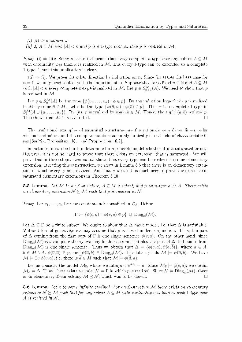
(i) M is κ-saturated.(ii) If A ⊆M with |A| < κ and p is a 1-type over A, then p is realized inM.
Proof. (i) ⇒ (ii): Being κ-saturated means that every complete n-type over any subset A ⊆ Mwith cardinality less than κ is realized in M. But every 1-type can be extended to a complete1-type. Thus, this implication is clear.
(ii) ⇒ (i): We prove the other direction by induction on n. Since (ii) states the base case forn = 1, we only need to deal with the induction step. Suppose that for a �xed n ∈ N and A ⊆Mwith |A| < κ every complete n-type is realized inM. Let p ∈ SMn+1(A). We need to show that pis realized inM.
Let q ∈ SMn (A) be the type {φ(v1, . . . , vn) : φ ∈ p}. By the induction hypothesis q is realizedinM by some a ∈ M . Let r be the type {ψ(a,w) : ψ(v) ∈ p}. Then r is a complete 1-type inSM1 (A ∪ {a1, . . . , an}). By (ii), r is realized by some b ∈ M . Hence, the tuple (a, b) realizes p.This shows thatM is κ-saturated.
The traditional examples of saturated structures are the rationals as a dense linear orderwithout endpoints, and the complex numbers as an algebraically closed �eld of characteristic 0,see [Sac72a, Proposition 16.1 and Proposition 16.2].
Sometimes, it can be hard to determine for a concrete model whether it is κ-saturated or not.However, it is not so hard to prove that there exists an extension that is saturated. We willprove this in three steps. Lemma 5.5 shows that every type can be realized in some elementaryextension. Iterating this construction, we show in Lemma 5.6 that there is an elementary exten-sion in which every type is realized. And �nally we use this machinery to prove the existence ofsaturated elementary extensions in Theorem 5.10.
5.5 Lemma. LetM be an L-structure, A ⊆M a subset, and p an n-type over A. There existsan elementary extension N �M such that p is realized in N .
Proof. Let c1, . . . , cn be new constants not contained in LA. De�ne
Γ := {φ(c, a) : φ(v, a) ∈ p} ∪ Diagel(M).
Let ∆ ⊆ Γ be a �nite subset. We ought to show that ∆ has a model, i.e. that ∆ is satis�able.Without loss of generality we may assume that p is closed under conjunction. Thus, the partof ∆ coming from the �rst part of Γ is one single sentence φ(c, a). On the other hand, sinceDiagel(M) is a complete theory, we may further assume that also the part of ∆ that comes fromDiagel(M) is one single sentence. Thus we obtain that ∆ = {φ(c, a), ψ(a, b)}, where a ∈ A,b ∈ Mr A, φ(v, a) ∈ p, and ψ(a, b) ∈ Diagel(M). The latter yields M |= ψ(a, b). We haveM |= ∃v φ(v, a), i.e. there is d ∈M such thatM |= φ(d, a).
Let us consider the model Mc, where we interpret cMc = d. Since Mc |= φ(c, a), we obtain
Mc |= ∆. Thus, there exists a model N |= Γ in which p is realized. Since N |= Diagel(M), thereis an elementary L-embeddingM� N , which was to be shown.
5.6 Lemma. Let κ be some in�nite cardinal. For an L-structureM there exists an elementaryextension N �M such that for any subset A ⊆M with cardinality less than κ, each 1-type overA is realized in N .

Types and Saturated Models 33
Proof. Let (pα : α < ζ) be an enumeration of all 1-types in SM1 (A) for all subsets A ⊆M with|A| < κ for some su�ciently large ordinal number ζ. We build an elementary chain of models(Mα : α < ζ):
Let M0 := M. If Mα is already constructed, then let Mα+1 be the elementary extensionof Mα in which pα is realized. This elementary extension exists by Lemma 5.5. For a limitordinal λ letMλ :=
⋃α<λMα. Proposition 2.11 assures that the union of an elementary chain
of models is an elementary extension of each member of the chain. Let
N :=⋃α<ζ
Mα.
Then every 1-type is realized in N . Again by Proposition 2.11, Mα � M for each α < ζ and,hence,M� N .
5.7 Corollary. In the situation of Lemma 5.6, also each n-type for n ∈ N is realized in N .
Proof. This follows immediately from Lemma 5.4.
We will now show that for each regular in�nite cardinal κ, every structure has an elementaryextension that is κ-saturated. A reader that is not familiar with set theory and regular cardinalsmay as well imagine any in�nite successor cardinal instead, since every in�nite successor cardinalnumber is regular, see [Del, Theorem 3.8.6]. For the sake of completeness we give the de�nitionof regularity:
5.8 De�nition. Let (B,<) be a totally ordered set. A subset A ⊆ B is called co�nal in B ifand only if for all b ∈ B there exists a ∈ A such that a > b. The co�nality of B, denoted bycf(B), is the least cardinal κ such that there exists a subset C ⊆ B which has cardinality κ andis co�nal in B.
5.9 De�nition. An in�nite cardinal κ is said to be regular if cf(κ) = κ.
5.10 Theorem. Let κ be a regular in�nite cardinal andM a model of a theory T . There existsa κ-saturated N |= T such thatM� N .
Proof. We build an elementary chain (Nα : α < κ), such that its limit will be the desiredκ-saturated elementary extension N : Let N0 :=M. Assuming that Nα is already constructed,let Nα+1 be the elementary extension of Nα such that for any subset A ⊆ M with cardinalityless than κ, any 1-type over A is realized in Nα+1. Such an extension exists by Lemma 5.6. Fora limit ordinal λ, we set
Nλ :=⋃α<λ
Nα.
By Proposition 2.11, Nλ is an elementary extension of every Nα. We �nally set
N :=⋃α<κ
Nα.
Again, by Proposition 2.11, N is an elementary extension of each Nα.It remains to show that N is κ-saturated. Let A ⊆ N with |A| < κ, and let p be an n-type
over A for some n ∈ N. Since κ is regular, its co�nality is equal to itself. Now the cardinality of

34 Quanti�er Elimination by Types and Saturation
A is smaller than κ. Hence, A cannot be co�nal in N , which implies that |A| is already containedin some Nα. Since every 1-type is realized in Nα, by Lemma 5.4 also every n-type for any n ∈ N,in particular p, is realized in Nα. Since Nα � N , this shows that N is κ-saturated.
5.11 Lemma. Let κ be an in�nite cardinal, M and N two models of a theory T , where M isκ-saturated and |N | ≤ κ, and let A ⊆ N be a subset. Then, any partial elementary embeddingf : A→M extends to an elementary embedding of N intoM.
Proof. Let κ0 := |NrA| and (nα : α < κ0) be an enumeration of NrA. De�ne Aα := A∪ {nβ :
β < α} for each α < κ0. Then, A0 = A. We build a sequence of partial elementary embeddingsf0 ( f1 ( . . . ( fα ( . . . for α < κ0 with fα : Aα →M.
We want the desired map to be
f :=⋃α<κ0
fα.
By trans�nite induction we show that for every α < κ0, the map fα is partial elementary. Weset f0 := f , which is by assumption partial elementary. If α is a limit ordinal, let fα :=
⋃β<α fβ .
Then, given that all fβ are partial elementary, also fα is partial elementary, since it is the unionof partial elementary functions.
For the successor ordinals let fα be already constructed and partial elementary. We need toextend this to a map fα+1 that is also partial elementary. Since both fα and fα+1 coincide onAα, it remains to de�ne fα+1(nα). De�ne the set
Γ(v) := {φ(v, fα(a1), . . . , fα(am)) : N |= φ(nα, a1, . . . , am) where a1, . . . , am ∈ Aα}.
We will show that Γ(v) is a 1-type. For this, we need to show that Γ(v)∪Th(M) is satis�able.By the Compactness Theorem it su�ces to show that every �nite subset of Γ(v) ∪ Th(M) issatis�able. Let ∆ := {φ1(v, fα(a1)), . . . , φn(v, fα(an))} ⊆ Γ(v) be an arbitrary �nite subset. Ifwe show that there is an element m ∈ M , such that M |= φi(m, fα(ai)) for each i = 1, . . . , n,i.e.M |=
∨ni=1 φi(x, fα(ai)), we are done. Since Γ(v) is closed under conjunction, φ(v, fα(a)) :=∨n
i=1 φi(v, fα(ai)) ∈ Γ(v). Then, N |= ∃v φ(v, a). Since fα is partial elementary this impliesthatM |= ∃v φ(v, fα(a)). SinceM |= Th(M), ∆ ∪Th(M) is satis�able. Hence, Γ(v) ∪Th(M)is satis�able. Thus, we have shown that Γ(v) is a 1-type.
By Lindebaum's Theorem it can be extended to a complete type Γ(v)∗ ∈ SM1 (Aα). SinceM isκ-saturated, Γ(v)∗ is realized inM by some b ∈M . Because Γ(v) is fully contained in Γ(v)∗, alsothe type Γ(v) is realized by b. We set fα+1(nα) := b, i.e. fα+1 = fα ∪{(nα, b)}. By construction,fα+1 is a partial elementary embedding. Thus, we obtain an elementary map f : N →M by
f :=⋃α<κ
fα.
We are now ready to state and proof another quanti�er elimination criterion.
5.12 Theorem. Let L be a language containing at least one constant symbol and T an L-theory.Then the following are equivalent:
(i) T has quanti�er elimination.

Di�erentially Closed Fields 35
(ii) If M |= T , A ⊆ M , N |= T is |M |+-saturated, f : A→ N is a partial embedding, then fextends to an L-embeddingM→N .
Proof. (i) ⇒ (ii): Let φ be an L-formula and a ∈ A such that M |= φ(a). By quanti�erelimination there is a quanti�er-free formula ψ such that M |= ψ(a). Since f is a partialembedding and, thus, preserves quanti�er-free formulas, we obtain N |= ψ(a). Hence, N |= φ(a).This shows that f is partial elementary. By Lemma 5.11, f extends to an L-embedding fromMinto N .
(ii)⇒ (i): We will use the previous quanti�er elimination criterion from Theorem 3.3. SupposeM,N |= T , A is a common substructure ofM and N , and φ is a quanti�er-free formula. Furtherlet b ∈ M and a ∈ A such that M |= φ(b, a). We need to show that there is c ∈ N such thatN |= φ(c, a).
Let N ′ |= T be an elementary extension of N which is |M |+-saturated. Such an extensionexists by Theorem 5.10. Let f : A→ N ′ be the identity map on A. By assumption f extends toan L-embedding f : M → N ′. This yields N ′ |= φ(f(b), f(a)) and also N ′ |= φ(f(b), a), sincef(a) = a. Therefore, N ′ |= ∃v φ(v, a). Since N is an elementary substructure of N ′, we obtainN |= ∃v φ(v, a), as desired. Now the quanti�er elimination criterion from Theorem 3.3 yieldsthat T has quanti�er elimination, which was to be shown.
5.2 Di�erentially Closed Fields
Since ancient times mathematicians have investigated roots of polynomial equations. A longamount of time later, they began to consider di�erential equations. It was an important contri-bution of model theory to algebra to introduce the axiomatic notion of di�erentially closed �elds.They are to di�erential polynomial equations what algebraically closed �elds are to polynomialequations, cf. [Poi, page 71].
According to [Mar96, page 53], the �rst work on the model theory of di�erentially closed�elds was done by Abraham Robinson, whose work was in�uenced by earlier work of AbrahamSeidenberg.
After giving a brief introduction to di�erential �elds, we will axiomatize the theory of di�er-entially closed �elds and use the above criterion from Theorem 5.12 to show that this theoryadmits quanti�er elimination. If not stated di�erently, we stick very closely to [Mar02, pages148�151].
5.13 De�nition. A derivation on a commutative ring R is a map δ : R → R such that theLeibniz rule holds:
δ(x+ y) = δ(x) + δ(y)
δ(xy) = xδ(y) + yδ(x).
We will write a′, a′′, . . . instead of δ(a), δ(δ(a)), . . . and we denote the nth derivative of a by a(n).
The Leibniz rules yield a way to extend the derivation on a ring to its �eld of fraction: Namelythe quotient rule
δ
(x
y
)=y · δ(x)− x · δ(y)
y2.

36 Quanti�er Elimination by Types and Saturation
5.14 De�nition. A di�erential �eld (K, δ) is a �eld K equipped with a derivation δ : K → K.We de�ne the ring of di�erential polynomials over K to be the following polynomial ring inin�nitely many variables:
K{X} = K[X, δ(X), δ2(X), . . . , δm(X), . . .].
If the corresponding derivation is clear, we will simply writeK instead of (K, δ). We can extendδ to a derivation on K{X} by setting δ(δn(X)) := δn+1(X). As above, we write δn(X) = X(n).
5.15 De�nition. A di�erential �eld isomorphism ψ : K → K ′ between two di�erential �elds(K, δ) and (K ′, δ′) is a �eld isomorphism that preserves the derivation. That means for everyk ∈ K we have ψ(δ(k)) = δ′(ψ(k)). Similarly a di�erential �eld embedding ψ : K → K ′ is a �eldembedding which preserves the derivation.
We will only consider �elds of characteristic 0 with one single derivation. One could alsoinvestigate the theory DCFp of di�erentially closed �elds of characteristic p > 0. This theory ismuch less well-behaved [Sac72b]. In [Gra] however, the author shows that the theory m-DCFof di�erentially closed �elds of characteristic 0 which have m many commuting derivations hasvery similar model theoretic properties to those of DCF: m-DCF admits quanti�er elimination[Gra, Theorem 3.1.7] and is complete [Gra, Theorem 3.1.9]. Henceforth, all �elds in this sectionwill be of characteristic 0 and equipped with one single derivation.
5.16 De�nition. Let (K, δ) be a di�erential �eld. For f ∈ K{X}rK, the order of f is thelargest n such that δn(X) occurs in f . If f is a constant, we say that f has order −∞.
In case f ∈ K{X} has order n, we can write
f(x) =
m∑i=0
gi
(X,X ′, . . . , X(n−1)
)(X(n)
)i,
where gi ∈ K[X,X ′, . . . , X(n−1)]. If gm 6= 0, we say that f has degree m.
5.17 De�nition. If k ⊆ K are di�erential �elds equipped with the same derivation δ, anda ∈ K, we denote by k〈a〉 the di�erential sub�eld of K generated by a over k.
5.18 Lemma. Let k ⊆ K be di�erential �elds of characteristic 0 and f ∈ k{X}r{0} be of ordern. Let a, b ∈ K with f(a) = f(b) = 0 such that a, . . . , a(n−1) are algebraically independent overk, and b, . . . , b(n−1) are algebraically independent over k, and g(a) 6= 0, g(b) 6= 0 for any g oforder n of lower degree in X(n). Then, there is a di�erential �eld isomorphism between k〈a〉 andk〈b〉 that �xes k.
Proof. A brief sketch of this proof can be found in [Mar02, Proposition 4.3.30 i)], here we presentmore detail.
The elements a, . . . , a(n−1) and b, . . . , b(n−1) are algebraically independent over k. This means,by sending a(i) to b(i) for each i < n, k(a, . . . , a(n−1)) and k(b, . . . , b(n−1)) are clearly isomorphicover k as �elds. Let us call this isomorphism ψ.
Further, f(a) = f(b) = 0 and every di�erential polynomial g of order n and lower degree inX(n) vanishes neither in a nor in b. There is a polynomial f ∈ k[X0, . . . , Xn] such that f(a) =f(a, . . . , a(n)). It holds f(a, . . . , a(n−1), t) ∈ k(a, . . . , a(n−1))[t] and by dividing it by a constant

Di�erentially Closed Fields 37
from k(a, . . . , a(n−1)), we may assume without loss of generality that it is a monic polynomial.Hence, f(a, . . . , a(n−1), t) is the minimal polynomial of a(n) over k(a, . . . , a(n−1)). Similarly,f(b, . . . , b(n−1), t) ∈ k(b, . . . , b(n−1))[t] is the minimal polynomial of b(n) over k(b, . . . , b(n−1)). Byapplying the isomorphism ψ to the coe�cients of the former minimal polynomial, one obtainsthe latter. Hence, also k(a, . . . , a(n)) and k(b, . . . , b(n)) are isomorphic as �elds. Since thisisomorphism extends ψ, we will keep its name.
In order to see that ψ extends to an isomorphism from k〈a〉 = k(a, . . . , a(n), . . .) into k〈b〉 =k(b, . . . , b(n), . . .), we will show that δ(a(n)) and δ(b(n)) can be expressed only using terms of lowerorder:
For all i < n we already have that δ(a(i)) = a(i+1) and δ(b(i)) = b(i+1). Let
f(x) =n∑i=0
m∑j=0
ci,j(x(i))j .
Di�erentiating yields
δ(f(a)) = δ
n∑i=0
m∑j=0
ci,j
(a(i))j
=
n∑i=0
m∑j=0
δ
(ci,j
(a(i))j)
=n∑i=0
m∑j=0
(δ(ci,j)
(a(i))j
+ ci,jj(a(i))j−1
a(i+1)
)
= f δ(a) +n∑i=0
∂f
∂X(i)(a)a(i+1),
where f δ is the polynomial obtained by di�erentiating the coe�cients of f and ∂f∂X(n) denotes
the nth partial derivative of f with respect to X(n). Since ∂f∂X(n) has lower degree in X(n) than
f , by assumption, it holds ∂f∂X(n) (a) 6= 0. Because f(a) = 0, and also δ(f(a)) = 0, it follows
−f δ(a) =n∑i=0
∂f
∂X(i)(a)δ(a(i)),
which is equivalent to
δ(a(n)) =
−f δ(a)−n−1∑i=0
∂f∂X(i) (a)δ(a(i))
∂f∂X(n) (a)
. (5.1)
Similarly we get
δ(b(n)) =
−f δ(b)−n−1∑i=0
∂f∂X(i) (b)δ(b(i))
∂f∂X(n) (b)
. (5.2)
Since both (5.1) and (5.2) use only terms of lower order to express δ(a(n)) and δ(b(n)), wehave shown that k(a, . . . , a(n), . . .) and k(b, . . . , b(n), . . .) are isomorphic as �elds. Again, this

38 Quanti�er Elimination by Types and Saturation
isomorphism will be called ψ. What remains to be shown is that under ψ, the derivation ispreserved. For this we will �rst show that for each k ∈ N it holds ψ(δ(a(k))) = δ(ψ(a(k))).Afterwards we will conclude that the equation also holds for every c ∈ k〈a〉.Let k ∈ {0, . . . , n − 1}. Since ψ(a(k+1)) = b(k+1), it holds ψ(δ(a(k))) = ψ(a(k+1)) = b(k+1) =
δ(b(k)) = δ(ψ(a(k))). The case where k ≥ n, reduces to the former by considering the equations(5.1) and (5.2).
Now, let c ∈ k〈a〉. Then there is f, g ∈ k[X0, . . . , Xm] for some m such that
c =f(a, . . . , a(m))
g(a, . . . , a(m))
and for the derivation it holds
δ(c) =δ(f(a, . . . , a(m)))g(a, . . . , a(m))− f(a, . . . , a(m))δ(g(a, . . . , a(m)))
g(a, . . . , a(m))2.
Hence, by applying the isomorphism ψ we obtain
ψ(δ(c)) =ψ(δ(f(a, . . . , a(m)))g(a, . . . , a(m))− f(a, . . . , a(m))δ(g(a, . . . , a(m)))
)ψ(g(a, . . . , a(m))2
)=ψ(δ(f(a, . . . , a(m)))
)ψ(g(a, . . . , a(m))
)− ψ
(f(a, . . . , a(m))
)ψ(δ(g(a, . . . , a(m)))
)ψ(g(a, . . . , a(m))
)2 .
Since ψ has the homomorphic property one can move ψ into the polynomials f and g, such thatit is only applied to the elements a, . . . , a(m). But for those elements we already have shown thatψ commutes with the derivation. Thus, we obtain ψ(δ(c)) = δ(ψ(c)).
Hence, we have shown that the ψ is indeed a di�erential �eld isomorphism.
5.19 De�nition. Let k ⊆ K be di�erential �elds. We say that a ∈ K is di�erentially algebraicover k if f(a) = 0 for some nonzero f ∈ k{X}. Otherwise a is di�erentially transcendental.
5.20 Lemma. Let k ⊆ K be di�erential �elds. If a ∈ K is di�erentially algebraic over k, thenthere is a nonzero di�erential polynomial f such that f(a) = 0 and for all g ∈ k{X}r {0} oflower order it holds that g(a) 6= 0. Moreover, one can choose f such that if there is b ∈ K withf(b) = 0 and g(b) 6= 0 for any lower order g, then k〈a〉 and k〈b〉 are isomorphic over k.
Proof. See [Mar02, Proposition 4.3.30 ii)]. Let a ∈ K be di�erentially algebraic over k. Let n beminimal such that a, . . . , a(n) are algebraically dependent over k, and let f ∈ k{X} be of order nand of minimal degree in X(n) such that f(a, . . . , a(n)) = 0. Obviously, g(a) 6= 0 for any nonzerog ∈ k{X} of order less than n.If f(b) = 0 and g(b) 6= 0 for any lower order polynomial g, then b, . . . , b(n−1) are alge-
braically independent over k. So b(n) is zero of the irreducible polynomial f(b, . . . , b(n−1), Y ) ∈k(b, . . . , b(n−1))[Y ]. Now, since all the assumptions of Lemma 5.18 are ful�lled, we conclude thatk〈a〉 and k〈b〉 are isomorphic over k.
5.21 De�nition. A di�erential �eld K is di�erentially closed if, whenever f, g ∈ K{X}, g isnonzero and the order of f is greater than the order of g, there is a ∈ K such that f(a) = 0 andg(a) 6= 0.

Di�erentially Closed Fields 39
That means in particular, if f has order zero, i.e. f ∈ K[X], there is a ∈ K with f(a) = 0.Hence, every di�erentially closed �eld is algebraically closed.
There are many examples of di�erential �elds: the �eld of formal power series K((X)) for some�eld K with its usual derivation, or the �eld of meromorphic functions on an open connectedsubset of C. These, and further examples can be found for instance in [Poi, page 71]. However,there is no natural example of a di�erentially closed �eld.
In the following we will show that every di�erential �eld can be embedded into a di�erentiallyclosed �eld. This part will be based on [Mar96, Section 1]. For a long time it was not clear ifthe di�erential closure is somehow unique like the algebraic or the real closure. Saharon Shelahhas shown that it is indeed unique up to isomorphism, cf. [Sac72a]

40 Quanti�er Elimination by Types and Saturation
5.22 De�nition. An ideal I � K{X} is called a di�erential ideal if for every f ∈ I it alsocontains its derivative. By 〈f〉 we denote the di�erential ideal generated by f . A prime di�erentialideal I ⊆ K{X} is a di�erential ideal which is also a prime ideal, i.e. if ab ∈ I for some a, b ∈ K,then a ∈ I or b ∈ I. Moreover, for a di�erential polynomial f ∈ K{X} we de�ne
I(f) :=
{h ∈ k{X} :
∂m
∂mX(n)h ∈ 〈f〉 for some m ∈ N
}.
Even if f is irreducible, 〈f〉 may not be prime. For example if f(X) = (X ′′)2 − 2X ′. Thenδ(f(X)) = 2X ′′ · X ′′′ − 2X ′′ = 2X ′′(X ′′′ − 1) is in 〈f〉, but neither 2X ′′ nor X ′′′ − 1 is in 〈f〉.But, however, the following holds:
5.23 Lemma. If f is an irreducible di�erential polynomial, then I(f) is a di�erential primeideal.
Proof. This proof is not trivial and needs some additional theory. We refer to [Poi, Lemma 6.10]or [Mar96, Corollary 1.7].
5.24 Theorem. Every di�erential �eld k has an extension K which is di�erentially closed.
Proof. [Mar96, Lemma 2.2] Let f ∈ k{X} be of order n and g ∈ k{X} of order less than n.By taking an irreducible factor of f of order n, we may as well assume that f is irreducible. Itfollows that g /∈ I(f), since g has order less than f .
By Lemma 5.23, I(f) is a di�erential prime ideal. Thus, let F be the fraction �eld F :=Quot(k{X}/I(f)). To see that δ is well-de�ned on F , let p, q ∈ k{X} with p− q ∈ I(f). Thenalso δ(a)− δ(b) = δ(a− b) ∈ I(f), as 〈f〉 is closed under di�erentiation. By the quotient rule, δextends to F .
Hence, let a ∈ F be the image of X mod I(f). Since f ∈ I(f), f(a) = 0 in F , while g /∈ I(f)yields g(a) 6= 0.
Iterating this process we can build K ⊇ k a di�erentially closed �eld.
We have now developed the theory of di�erential �elds that is needed for the proof of quanti�erelimination of di�erentially closed �elds. We will proceed by giving an axiomatization of DCF.The theory of di�erential �elds is given by the axioms for �elds of characteristic 0 together withthe Leibniz rule. In order to formalize that a di�erential �eld is di�erentially closed we needadditionally a countable in�nite family of axioms. It is di�cult to write down a general axiomas there are many varying parameters: the orders of the two polynomials and the degree ofthem in every �variable � X(i). We will not use any axioms, the important point for us is thatone is convinced that there exists an axiomatization. But this is not hard to see, since we caneasily formalize di�erential polynomials and the fact that there exists an element in which onedi�erential polynomial vanishes and the other one does not.
5.25 De�nition. Let L be the language 〈+ ,− , · , δ ; 0 , 1〉, where δ is a unary function symbolfor the derivation. The theory DCF of di�erentially closed �elds is axiomatized as follows:
� the �eld axioms K1 to K9,
� characteristic 0: For each n ∈ N we have:

Di�erentially Closed Fields 41
K0n: ∀x ((x+ . . .+ x︸ ︷︷ ︸n times
= 0)→ x = 0)
� the Leibniz rule for di�erentiation:
D1: ∀x∀y δ(x+ y) = δ(x) + δ(y),D2: ∀x∀y δ(x · y) = xδ(y) + yδ(x).
� and additionally di�erential closedness: For any non-constant di�erential polynomials fand g where the order of g is less than the order of f , there exists an x such that f(x) = 0and g(x) 6= 0.
5.26 Theorem. The theory of di�erentially closed �elds admits quanti�er elimination.
Proof. See [Mar02, Theorem 4.3.32]. Suppose that K |= DCF is a di�erentially closed �eld,R ⊆ K a subset, M |= DCF |K|+-saturated. Let f : R → M be a partial embedding. Aswe will see in Chapter 6, without loss of generality, by Lemma 6.2, we may assume that R is asubstructure of K, i.e. the substructure R ⊆ K that is generated by R, that means the smallestsubstructure of K which contains R. Hence, R is a di�erential subring of K and f is a di�erentialring embedding, that means a ring embedding which preserves the derivation. In order to applyTheorem 5.12, we must show that f extends to a di�erential �eld embedding of K intoM.
Surely, f extends to a di�erential �eld embedding of Quot(R) intoM, since there is a uniqueextension of the derivation from R to Quot(R). Therefore, we may assume that R is already a�eld. If we show that for every a ∈ Kr R, there is a di�erential �eld embedding of R〈a〉 intoM, then by trans�nite induction we are done. By identifying R with f(R) we may assume thatR ⊆M and that f is the identity onR. Now, a is either di�erentially algebraic or transcendentalover R. We consider both cases:
Case 1: a is di�erentially algebraic over R. Let f ∈ R{X}r {0} be as in Lemma 5.20. Let nbe the order of f . Let p be the type {f(v) = 0} ∪ {g(v) 6= 0 : g is nonzero of order less than n}.If g1, . . . , gm are nonzero di�erential polynomials of order less than n, then gi(a) 6= 0 for all i,while f(a) = 0. Therefore, there exists s ∈ M such that f(s) = 0 and
∏mi=1 gi(s) 6= 0. Thus,
p is satis�able, and since M is |K|+-saturated, p is realized by some b ∈ M . Since g(b) 6= 0for all nonzero di�erential polynomials g of order less than n, it follows that b, b′, . . . , b(n−1) arealgebraically independent over R. Also a, a′, . . . , a(n−1) are algebraically independent over R, soby Lemma 5.18, R〈a〉 and R〈b〉 are isomorphic over R. Thus, we can extend the di�erential �eldembedding by sending a to b.
Case 2: a is di�erentially transcendental over R. Let p be the type {g(v) 6= 0 : g ∈ R{X}r{0}}.Let g1, . . . , gn ∈ R{X}r {0}. Let N := max{deg(gi) : i = 1, . . . , n} + 1 and let f(x) = x(N).Since M is di�erentially closed, there is s ∈ M such that f(s) = s(N) = 0 and gi(s) 6= 0 forall i = 1, . . . , n. Thus, p is satis�able and, by |K|+-saturation, realized by some b ∈ M that isdi�erentially transcendental over R. Since R〈a〉 and R〈b〉 are over R isomorphic to the fraction�eld QuotR{X}, we can extend the di�erential �eld embedding again by sending a to b.

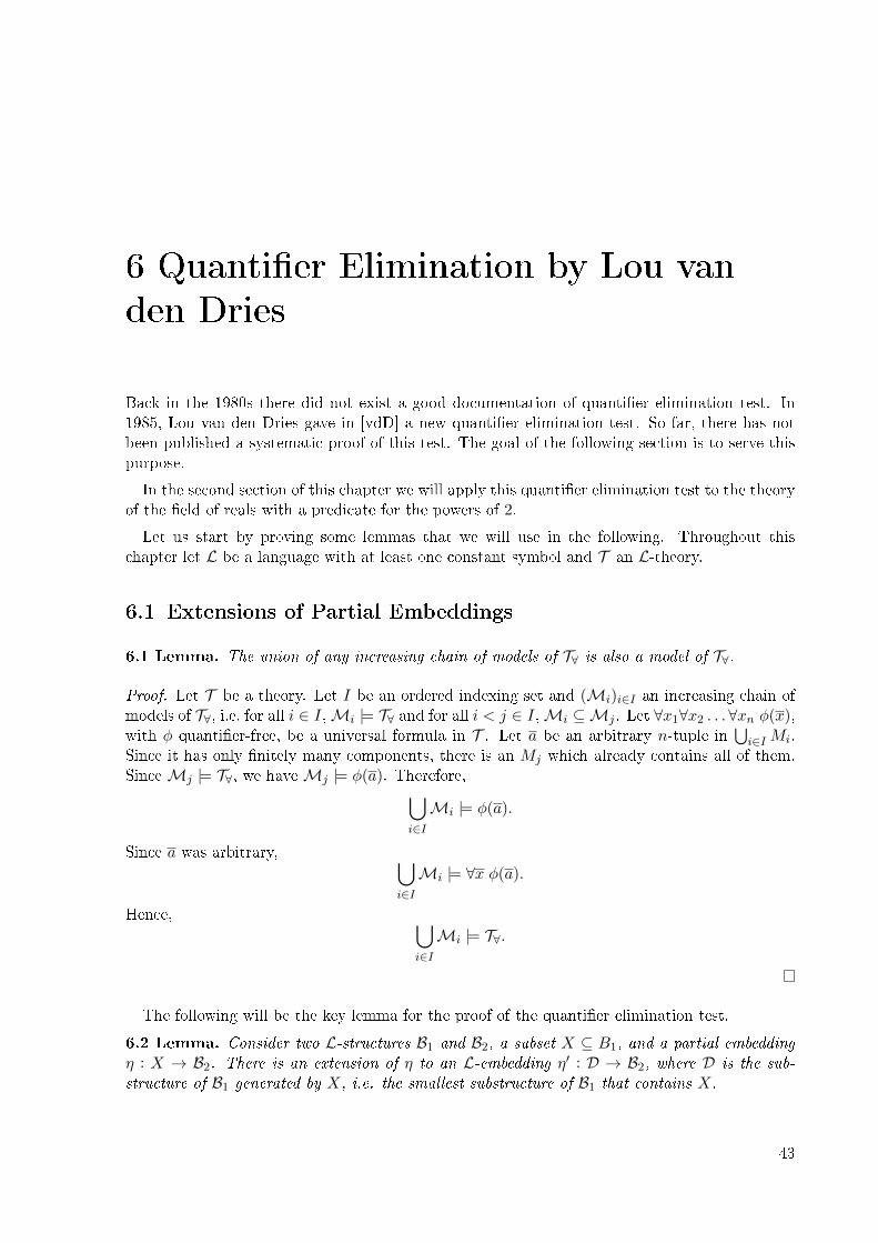
6 Quanti�er Elimination by Lou van
den Dries
Back in the 1980s there did not exist a good documentation of quanti�er elimination test. In1985, Lou van den Dries gave in [vdD] a new quanti�er elimination test. So far, there has notbeen published a systematic proof of this test. The goal of the following section is to serve thispurpose.
In the second section of this chapter we will apply this quanti�er elimination test to the theoryof the �eld of reals with a predicate for the powers of 2.
Let us start by proving some lemmas that we will use in the following. Throughout thischapter let L be a language with at least one constant symbol and T an L-theory.
6.1 Extensions of Partial Embeddings
6.1 Lemma. The union of any increasing chain of models of T∀ is also a model of T∀.
Proof. Let T be a theory. Let I be an ordered indexing set and (Mi)i∈I an increasing chain ofmodels of T∀, i.e. for all i ∈ I,Mi |= T∀ and for all i < j ∈ I,Mi ⊆Mj . Let ∀x1∀x2 . . . ∀xn φ(x),with φ quanti�er-free, be a universal formula in T . Let a be an arbitrary n-tuple in
⋃i∈IMi.
Since it has only �nitely many components, there is an Mj which already contains all of them.SinceMj |= T∀, we haveMj |= φ(a). Therefore,⋃
i∈IMi |= φ(a).
Since a was arbitrary, ⋃i∈IMi |= ∀x φ(a).
Hence, ⋃i∈IMi |= T∀.
The following will be the key lemma for the proof of the quanti�er elimination test.
6.2 Lemma. Consider two L-structures B1 and B2, a subset X ⊆ B1, and a partial embeddingη : X → B2. There is an extension of η to an L-embedding η′ : D → B2, where D is the sub-structure of B1 generated by X, i.e. the smallest substructure of B1 that contains X.
43

44 Quanti�er Elimination by Lou van den Dries
Proof. We will �rst explain how to construct D, the substructure of B1 generated by X. Secondlywe will show that η can be extended to an L-embedding from D into B2. What we need to do isadd to X all the elements that arise from applying terms to every tuple x ∈ X and de�ne whathappens to them when applying f .
Set D := {tB1(x) : t is a term and x ∈ X}. Then D is closed under terms. For every constantc ∈ L, let cD := cB1 . To see that cD is an element of D, consider the term t = c, then tB1 ∈ D,thus cD ∈ D.
Let g(v) be an r-ary function symbol in B1. For d ∈ D de�ne gD(d) := gB1(d). Now d is notnecessarily a tuple in X. However, it was constructed by a term. Thus, let t1, . . . , tr be termssuch that d = (d1, . . . , dr) = (tB11 (x1), . . . , t
B1r (xr)) for some x1, . . . , xr ∈ X, and let t(v1, . . . , vr)
be the term g(t1(v1), . . . , tr(vr)). Therefore, gD(d) = tB1(x1, . . . , xr) ∈ D.
For a relation symbol R we de�ne D |= RD(d) if and only if B1 |= RB1(d).
Since the L-embedding is the identity map on D into B1, it is injective. Thus, by construction,D is a substructure of B1.Now let η : X → B2 be a partial embedding. For any d ∈ D, say d = tD(x) for some term t, and
some tuple x ∈ X, we de�ne η′(tD(x)) := tB2(η(x)). For d ∈ D the choice of a term t such thatd = tD(x) might not be unique. In order to see well-de�nedness, note that D |= t1(x) = t2(x) forx ∈ X immediately yields that B2 |= t1(η(x)) = t2(η(x)), since η is a partial embedding. Hence,η′ is well-de�ned. We claim that η′ is an L-embedding.For a constant symbol c in L we have η′(cD) = η′(cB1) = cB2 . Let f be a function symbol.
Then:
η(fD(tD1 (x1), . . . , tDn (xn))) = η((fD(tD1 , . . . , t
Dn ))(x1, . . . , xn))
= fB2(tB21 , . . . , tB2n )(η(x1), . . . , η(xn))
= fB2(tB21 (η(x1)), . . . , tB2n (η(xn)))
= fB2(η′(tD1 (x1)), . . . , η′(tDn (xn))).
Let R be a relation symbol in L. Then the following are equivalent:
D |= R(t1(x1), . . . , tn(xn))
⇔ B1 |= R(t1(x1), . . . , tn(xn)) since D ⊆ B1⇔ B2 |= R(t1(x1), . . . , tn(xn)) since R(t1, . . . , tn) is quanti�er-free
and x1, . . . , xn ∈ X⇔ B2 |= R(η′(t1(x1)), . . . , η
′(tn(xn))) by de�nition of η′
Hence, we have shown that η′ is, indeed, an L-embedding.
We will now come to van den Dries' quanti�er elimination test, which he gave in [vdD]:
6.3 Theorem. Let T be a theory with at least one constant symbol and suppose that the followingconditions hold:
(1) Each model M of T∀ has a T -closure M. This means that for every M |= T∀ there isM |= T withM⊆M, andM can be embedded overM into each T -extension ofM, i.e.into every N |= T withM⊆ N .

Extensions of Partial Embeddings 45
(2) IfM ( N are models of T , then there is b ∈ NrM such thatM(b), the T∀-model generatedby b overM, can be embedded overM into an elementary extension ofM.
Then T admits quanti�er elimination.
Proof. We will prove this quanti�er elimination test by using Theorem 5.12 and by applying theprevious lemma several times.
LetM |= T be a model, X ⊆M a subset, N |= T an |M |+-saturated model, and f : X → Na partial embedding. We need to show that f extends to an L-embedding f :M→N . For thesake of simplicity, f will keep its name after each extension.
By Lemma 6.2, f extends to an L-embedding f : A → N , where A is the substructure ofMgenerated by the set X. Thus, A is a model of the universal theory T∀, by Lemma 2.13. We maynow apply condition (1). So, A has a T -closure, i.e. A ⊆ A |= T and A can be embedded overA into N . Thus, f extends to an L-embedding f ′ : A → N . Moreover, A is embedded over AintoM.
From this point we start a trans�nite iteration. Let f0 := f ′ and A0 := A. We will builda chain of models A0 ⊆ A1 ⊆ . . . ⊆ Aα ⊆ . . . ⊆ M and, as in Lemma 5.11, a chain of L-embeddings f0 ⊆ f1 ⊆ . . . ⊆ fα ⊆ . . ., where fα : Aα → N . Let κ = |Mr A|. We want thedesired map to be
f :=⋃α<κ
fα :M→N .
For the successor step suppose that Aα and fα : Aα → N are already constructed. Withoutloss of generality we assume that Aα (M, otherwise set Aα+1 = Aα and fα+1 = fα and we aredone.
By condition (2), there is an element bα ∈MrAα such that Aα(bα) can be embedded over Aαinto an elementary extension of Aα, say Eα. Applying condition (1) again, since Aα(bα) |= T∀,it has a T -closure Aα(bα) |= T that can be embedded over Aα(bα) into each T -extension ofAα(bα), in particular into Eα. Hence, we obtain the following diagram:
Aα
�
⊆ Aα(bα) ⊆ Aα(bα) ⊆ M.
⊇
Eα
We will �rst construct an L-embedding of Aα∪{bα} into N , then extend it to an L-embeddingfrom Aα(bα) into N , and �nally obtain one from Aα(bα) into N . Let fα+1
∣∣Aα = fα. De�ne the
set
Γ(v) := {φ(v, fα(a)) : a ∈ Aα, φ is a quanti�er-free formula, andM |= φ(bα, a)}.
In order to show that Γ(v) is a type, we need to demonstrate that Γ(v) ∪ Th(N ) is satis�able.Let ∆ ⊆ Γ(v) be an arbitrary �nite subset. We will show that there is x ∈ N such thatN |= φ(x, fα(a)) for each φ(v, fα(a)) ∈ ∆. This will imply that Γ(v) ∪ Th(N ) is satis�able.Since Γ(v) is closed under conjunction, we may assume that ∆ = {φ(v, fα(a))} only consists ofone single formula with a ∈ Aα. ThenM |= φ(bα, a) and it su�ces to show that φ(v, fα(a)) issatis�able in N . Since φ is quanti�er-free and bα ∈ Aα(bα) ⊆ M, we have Aα(bα) |= φ(bα, a),in other words Aα(bα) |= ∃v φ(v, a). Then also Eα |= ∃v φ(v, a). Since Eα is an elementaryextension of Aα and a ∈ Aα, we obtain Aα |= ∃v φ(v, a). By induction hypothesis, we already

46 Quanti�er Elimination by Lou van den Dries
have an L-embedding of Aα into N and existential formulas are preserved upwards in inclusion.This yields N |= ∃v φ(v, fα(a)).
Thus, we have shown that Γ(v)∪Th(N ) is satis�able and, hence, that Γ(v) is a 1-type whichcan be extended to a complete type Γ(v)∗ ∈ SN1 (Aα). Since N is |M |+-saturated, there is someelement cα ∈ N that realizes Γ(v)∗ and thus, Γ(v). Set fα+1(bα) = cα.
In order to convince oneself that fα+1 is still injective, suppose that N |= fα+1(bα) = fα+1(a)for a ∈ Aα+1. We will show that this implies already bα = a inM which proves injectivity. Letus have a look at the formula φ(v, w) that denotes the equality v = w. This is a quanti�er-freeformula. Thus, φ(v, fα+1(a)) ∈ Γ(v), i.e.M |= φ(bα, a). This yields thatM |= bα = a. Hence,we have a partial embedding of Aα ∪ {bα} into N .
By Lemma 6.2, it can be extended to an L-embedding from Aα(bα) into N , since Aα(bα) is thesmallest substructure ofM that contains Aα and bα. By condition (1), Aα(bα) can be embeddedover Aα(bα) into N . Hence, we have �nished the construction of fα+1. Set Aα+1 := Aα(bα).Then fα+1 : Aα+1 → N is an L-embedding of models.
For a limit ordinal α letf ′α :=
⋃λ<α
fλ :⋃λ<α
Aλ → N .
Since each fλ is an L-embedding, also their union f ′α is an L-embedding. EachAλ is, in particular,a model of T∀. By Lemma 6.1 their union is also a model of T∀ and by condition (1) this unionhas a T -closure ⋃
λ<α
Aλ =: Aα,
that can be embedded over⋃λ<αAλ into N . Thus, Aα |= T and f ′α expands to the L-embedding
fα : Aα → N .
This algorithm terminates as soon as Aα = M. At this point we obtain the desired L-embedding f := fα :M→N .
By Theorem 5.12, T admits quanti�er elimination.
6.2 The Field of Reals with a Predicate for the Powers of Two
In this chapter we will show that the theory of real closed �elds with a certain discrete multiplica-tive subgroup�in the following denoted by RPT�has quanti�er elimination in the language ofordered rings augmented by two new symbols. This section follows [vdD]. We will denote by Lthe language 〈+ ,− , · ;< ; 0 , 1〉 of ordered rings. For simplicity reasons, we will omit the symbolsof L when talking about a structure.
Let λ be a unary function symbol, A a unary relation symbol and for every n ∈ N, let Pn bea unary relation symbol. By L∗ we denote the language L ∪ {A, λ, Pn : n = 1, 2, . . .}.
6.4 De�nition. Let RPT, the theory of the �eld of reals with a predicate for the powers of two,as van den Dries calls it, be the L∗-theory given by the following axioms expressing that:
� R is a real closed ordered �eld, i.e. axioms K1 to K9, O1 to O5, RK1, and RK2n,
� A is a multiplicative subgroup of positive elements of R:
A1: ∀x (A(x)→ x > 0)
The Field of Reals with a Predicate for the Powers of Two 47
A2: ∀x∀y ((A(x) ∧A(y))→ A(x · y))A3: A(1)A4: ∀x (A(x)→ ∃y (A(y) ∧ x · y = y · x = 1)).

48 Quanti�er Elimination by Lou van den Dries
� such that:
V1: A(1 + 1),V2: ∀x (1 < x < 2→ ¬A(x)),
V3n: ∀x (Pn(x)↔ ∃y (A(y) ∧ yn = x)), for all n ∈ N,V4: ∀x (x ≤ 0→ λ(x) = 0),V5: ∀x (x > 0→ (A(λ(x)) ∧ λ(x) ≤ x < 2λ(x))).
Axiom V1 states that 2 ∈ A. Since A is a multiplicative group, it contains all powers of 2.By V1 there is no element in A between 1 and 2. For an element x it holds Pn(x) if and only ifx has an nth root which lies in A. The function λ assigns to each positive element y the nearestelement in A which is less than or equal to y. If y is not positive, then λ(y) = 0. Instead ofA(x), we will write x ∈ A in the following as usually.
We will prove the following theorem after we have developed some theory:
6.5 Theorem. The L∗-theory RPT admits elimination of quanti�ers.
First we will go a little into valuation theory. For this part, see [Kuh, pages 9, 15, and 16].
6.6 De�nition. We say that two nonzero elements a and b of an ordered �eld K are of the samearchimedean class if
1
n<∣∣∣ab
∣∣∣ < n
for some n ∈ N.
6.7 De�nition. Let K be a �eld and Γ an ordered abelian group. A valuation on K is asurjective map v : K → Γ ∪ {∞} which satis�es the following properties for all a, b ∈ K:
(i) v(a) =∞ if and only if a = 0,(ii) v(ab) = v(a) + v(b),(iii) v(a+ b) ≥ min{v(a), v(b)}.The value group of a valuation is the image v(K×).
There are some immediate consequences for a valuation v : K → Γ ∪ {∞}: For every a ∈ Kit holds v(−a) = v(a). For a 6= 0 we have v(a−1) = −v(a). Every �nite element�that meansevery element bounded by some natural number�has valuation 0: v(1) = v(1 · 1) = v(1) + v(1),hence, v(1) = 0. Now for any �nite element r, 1/r can be bounded by 1/n and n for somen > r, thus v(r) = 0. Condition (iii) also holds for more than two summands: v(a1 + . . .+an) ≥min{a1, . . . , an} for all n ∈ N and ai ∈ K. And �nally the inequality in (iii) is an equalityv(a+ b) = min{v(a), v(b)} if v(a) 6= v(b).
It is not hard to see that the property of being in the same archimedean class forms anequivalence relation. Let Γ be the set of archimedean classes of nonzero element in a �eld K.We denote by [a] the equivalence class of a. By setting [a] < [b] if and only if n|b| < |a| for everyn ∈ N, we can de�ne an order on Γ. One can easily check that the order is well-de�ned. We alsode�ne an addition on Γ by setting [a] + [b] := [ab]. Equipped with this operation and order, Γbecomes an ordered Abelian group with neutral element [1]. We also obtain the following:
6.8 Proposition. The map v : K → Γ ∪ {∞} given by a 7→ [a] for a ∈ K× and 0 7→ ∞, is avaluation. It reverses order on positive elements, i.e. 0 < a ≤ b implies that v(a) ≥ v(b).

The Field of Reals with a Predicate for the Powers of Two 49
Proof. We will check the conditions that makes a map into a valuation. It is certainly byde�nition surjective and (i) is ful�lled. Also (ii) holds by de�nition.
In order to verify (iii), let a, b ∈ K. If a = 0, then v(a) =∞ and v(a+ b) = v(b). Similarly forb = 0. So let a, b 6= 0. First assume that [a] < [b], and that both a and b are positive, as otherwiseone can simply consider their negatives. Together these assumptions yield that nb < a for alln ∈ N, in particular b < a. Then it holds a < a+ b ≤ n(a+ b) = na+ nb < na+ a = (n+ 1)a.Dividing by a yields
1
n+ 1< 1 <
a+ b
a< n+ 1.
Hence, [a+ b] = [a].
Now let [a] = [b] and assume that a ≥ b > 0. Further, assume that [a+b] < [a]. Then it followsfor all n ∈ N that na < a + b, in particular, 2a < a + b. But this yields a < b, a contradiction.Hence, [a+ b] ≥ [a] = [b]. This shows condition (iii).
What remains to be shown is that the valuation reverses order on positive elements. Leta, b ∈ K with a, b > 0. Suppose that a < b. This implies by de�nition of the order immediatelythat [a] ≥ [b]. Hence 0 < a ≤ b implies that v(a) ≥ v(b).
From now on, let v denote the above examined valuation, which assigns to each element itsarchimedean class. We will call this valuation in the following the natural valuation.
The natural valuation on K can be extended to the real closure K:
6.9 Lemma. Suppose that K is an ordered �eld. The natural valuation v : K → Γ ∪ {∞} canbe extended to the natural valuation v on the real closure K of K. It satis�es v : K → Γ ∪ {∞},where Γ is the divisible hull of Γ, and for all x ∈ K, it holds
v(x) =1
n· v(y)
for some y ∈ K, y > 0 and n > 0.
Proof. It is easy to see that v can be extended to K, since v∣∣K
= v. Let x ∈ Kr K. Letf(t) = ant
n + an−1tn−1 + . . . + a1t + a0 be the minimal polynomial of x over K with an = 1,
a0 6= 0, and ai ∈ K for every i ∈ {0, . . . , n}. Then anxn + an−1x
n−1 + . . . + a1x + a0 = 0.Applying the valuation, we obtain
v(anxn + an−1x
n−1 + . . .+ a1x) = v(−a0).
Without loss of generality we assume that for every i ∈ {0, . . . , n} it holds ai 6= 0, as otherwisewe consider only the indices of the nonzero monomials. Suppose that there is i > j such thatv(aix
i) = v(ajxj). This means that v(aj)−v(ai) = v(xi)−v(xj) and therefore v(xi−j) = v(aj/ai).
It follows that
v(x) =1
i− j· v(ajai
).
If aj/ai is negative, by replacing it with ai/aj instead, we obtain the claimed form.

50 Quanti�er Elimination by Lou van den Dries
If, however, the valuations of the monomials are pairwise di�erent, i.e. if for all i 6= j we havev(aix
i) 6= v(ajxj), we obtain
v(a0) = v(−a0)= min
i=1,...,n{v(aix
i)}
= mini=1,...,n
{v(ai) + v(xi)}
= mini=1,...,n
{v(ai) + i · v(x)}
Let i0 ∈ {0, . . . , n} such that v(ai0xi0) = mini=1,...,n{v(aix
i)}. Then v(a0) = v(ai0) + i0 · v(x)and therefore
v(x) =1
i0· v(a0ai0
).
As above, if a0/ai0 is not positive we may replace it by its negative. This proves the claim.
6.10 Lemma. Let K = (K,A, (Pn), λ) be a model of the universal theory RPT∀, and v thenatural valuation on K. Then the following holds:
(a) Each archimedean class of K is represented by an element in A. Thus, v(A) = Γ.(b) v
∣∣Ahas kernel 2Z.
(c) There is an isomorphism A/2Z ∼= Γ.
Proof. (a) For x > 0 we have λ(x) ≤ x < 2λ(x) and λ(x) 6= 0, i.e. 1/2 < 1 ≤ x/λ(x) < 2 byV5, that means that x and λ(x) are part of the same archimedean class. So each archimedeanclass is represented by an element of A, since im(λ) ⊆ A.(b) ⊆ : Let x ∈ A with v(x) = 0. As [x] = [1], there is n ∈ N such that 1/n < x < n. Let
k ∈ Z be minimal such that x < 2k+1 ≤ n. Then 2k ≤ x < 2k+1. This yields 1 ≤ x/2k < 2. Byaxiom V2 it follows that x/2k = 1, and thus, x = 2k.
⊇ : Since v(1) = 0 and 1/3 < 1/2 < 3, the numbers 1 and 2 are in the same archimedeanclass, i.e. v(2) = 0. Then also v(2k) = 0 for all k ∈ Z. And since 2Z ⊆ A, we are done.(c) By (a), every archimedean class has one representative from A. Hence, v
∣∣Ais is surjective.
Then the claim follows from (b) and the �rst isomorphism theorem.
From part (c) of Lemma 6.10 it follows that two elements in A which are in the samearchimedean class only di�er by a power of 2. This means that for a, b ∈ A with [a] = [b]there exists n ∈ Z such that a · 2n = b.
Consider a model (K,A, (Pn), λ) of the universal theory RPT∀. Depending on the structureof K we may draw di�erent conclusions: If K is a �eld, it follows that A is a group. This showsLemma 6.11. If, however, K is even real closed, then (K,A, (Pn), λ) is even a model of RPT.We will prove this in Lemma 6.12.
6.11 Lemma. Let K = (K,A, (Pn), λ) |= RPT∀, where K is a �eld. Then A and Pn are groupswith Pn ⊆ A.
Proof. Since K is a model of the universal theory, by Lemma 2.13, there is a model R =(R,B, (Qn), µ) |= RPT with K ⊆ R. Let us �x an arbitrary natural number n ∈ N. By

The Field of Reals with a Predicate for the Powers of Two 51
de�nition, B is a group. Clearly, Qn is closed under multiplication and, if x has an nth root yin B, then also 1/x has an nth root in B, namely 1/y. Hence, also Qn is a group. Because Kis a substructure of R, it holds A = B ∩ K. Now B is a group and K is a �eld, hence, theirintersection is also a group. Similarly, it follows that Pn = Qn ∩K is a group.
6.12 Lemma. Let K = (K,A, (Pn), λ) |= RPT∀, where K is a real closed �eld. Then K |= RPT.
Proof. Since K |= RPT∀, there is a model R = (R,B, (Qn), µ) |= Σ∗ such that K ⊆ R.Obviously, axioms K1�K9, O1�O5, RK1, and RK2n are satis�ed in K, since K is real
closed. By Lemma 6.11, A is an ordered Abelian group, hence also axioms A1�A4 hold. Now,V1, V2, V4, and V5 are universal, hence, preserved downwards in inclusion. They hold in R,therefore they also hold in K. It remains to show V3n. If x has an nth root in A, it is certainlycontained in Pn. So, let on the contrary x ∈ Pn. Then x ∈ Qn, which implies that there is y ∈ Bwith yn = x. Since K is real closed, y already lies in K. But K ∩ B = A. Hence, y ∈ A. Thisestablishes axiom V3n and �nishes the proof.
6.13 Lemma. Let K = (K,A, (Pn), λ) |= RPT∀. For each x ∈ A exactly one of x, 2x, . . . , 2n−1xbelongs to Pn.
Proof. By Lemma 2.13, there is R = (R,B, (Qn), µ) |= RPT with K ⊆ R. Since R is real closed,the value group of the natural valuation v on R is divisible and, therefore, by Lemma 6.10 (c),also B/2Z.
This means: For all n ∈ N and for all x ∈ B there exists b ∈ B such that bn2Z = x2Z. In otherwords: ∀n ∈ N ∀x ∈ B ∃b ∈ B ∃` ∈ Z :
bn = x2`.
What remains to be shown is that ` can be chosen to be ` ∈ {0, . . . , n − 1} and is unique: Bydivision with remainder we obtain ` = rn + k where k ∈ {0, . . . , n − 1} is unique, so bn =x · 2k · (2r)n. Set b = b · 2−r. This yields bn = (b · 2−r)n = x · 2k.Formalizing what we have just shown, this gives us the analogue of axiomP4n from Presburger
Arithmetic:
R |= ∀x
B(x)→n−1∨i=0
(Qn(2ix) ∧
∧j 6=i¬Qn(2jx)
) for all n ∈ N.
But this is a universal L∗-formula, hence, preserved downwards in inclusion. Thus, it alsoholds
K |= ∀x
A(x)→n−1∨i=0
(Pn(2ix) ∧
∧j 6=i¬Pn(2jx)
) for all n ∈ N.
This proves the claim.
The reader may have noticed some analogues to Presburger Arithmetic. In fact, the theoryRPT somehow extends Pr:
6.14 Proposition. Let K = (K,A, (Pn), λ) be a model of RPT. Then A = (A, ·,÷, <, 1, 2, (Pn))is a model of Presburger Arithmetic.
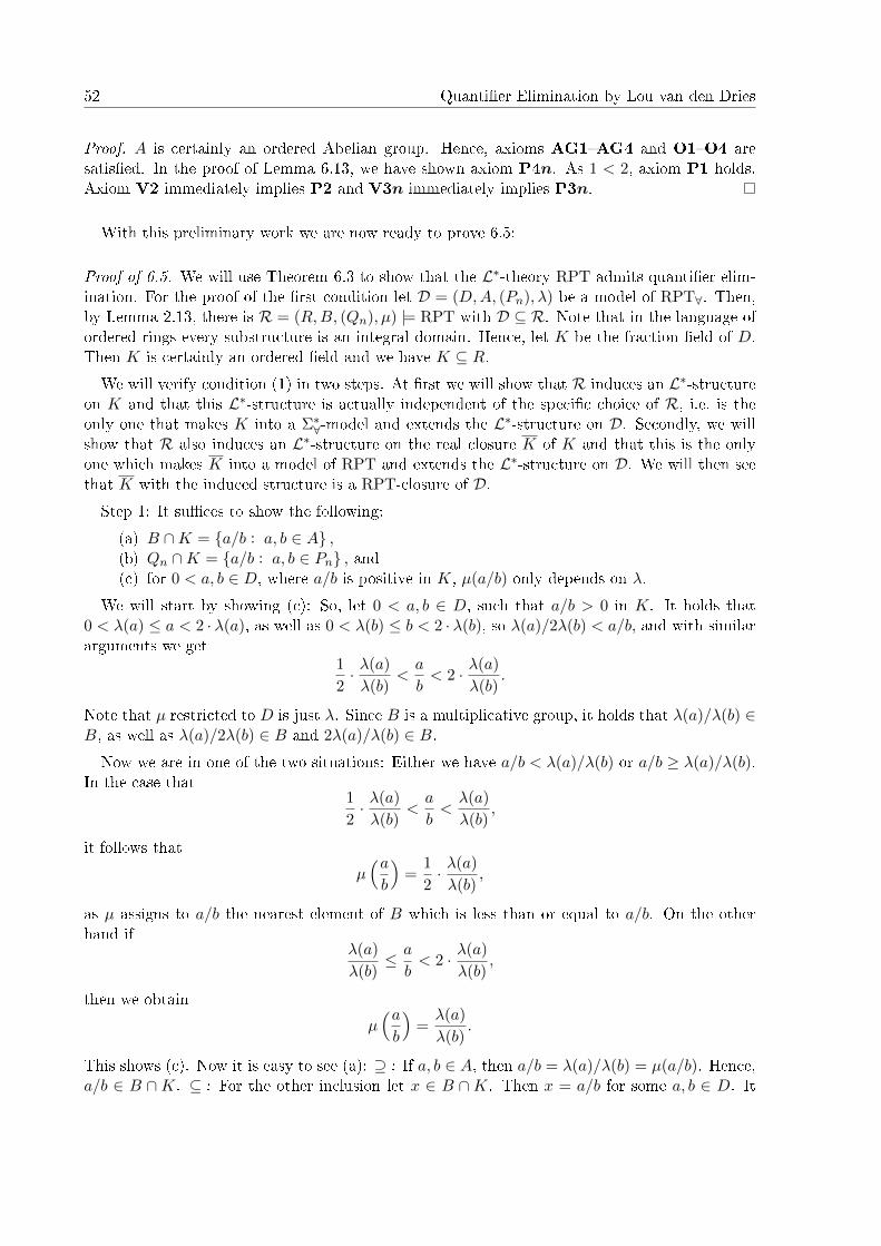
52 Quanti�er Elimination by Lou van den Dries
Proof. A is certainly an ordered Abelian group. Hence, axioms AG1�AG4 and O1�O4 aresatis�ed. In the proof of Lemma 6.13, we have shown axiom P4n. As 1 < 2, axiom P1 holds.Axiom V2 immediately implies P2 and V3n immediately implies P3n.
With this preliminary work we are now ready to prove 6.5:
Proof of 6.5. We will use Theorem 6.3 to show that the L∗-theory RPT admits quanti�er elim-ination. For the proof of the �rst condition let D = (D,A, (Pn), λ) be a model of RPT∀. Then,by Lemma 2.13, there is R = (R,B, (Qn), µ) |= RPT with D ⊆ R. Note that in the language ofordered rings every substructure is an integral domain. Hence, let K be the fraction �eld of D.Then K is certainly an ordered �eld and we have K ⊆ R.We will verify condition (1) in two steps. At �rst we will show that R induces an L∗-structure
on K and that this L∗-structure is actually independent of the speci�c choice of R, i.e. is theonly one that makes K into a Σ∗∀-model and extends the L∗-structure on D. Secondly, we willshow that R also induces an L∗-structure on the real closure K of K and that this is the onlyone which makes K into a model of RPT and extends the L∗-structure on D. We will then seethat K with the induced structure is a RPT-closure of D.Step 1: It su�ces to show the following:
(a) B ∩K = {a/b : a, b ∈ A} ,(b) Qn ∩K = {a/b : a, b ∈ Pn} , and(c) for 0 < a, b ∈ D, where a/b is positive in K, µ(a/b) only depends on λ.
We will start by showing (c): So, let 0 < a, b ∈ D, such that a/b > 0 in K. It holds that0 < λ(a) ≤ a < 2 · λ(a), as well as 0 < λ(b) ≤ b < 2 · λ(b), so λ(a)/2λ(b) < a/b, and with similararguments we get
1
2· λ(a)
λ(b)<a
b< 2 · λ(a)
λ(b).
Note that µ restricted to D is just λ. Since B is a multiplicative group, it holds that λ(a)/λ(b) ∈B, as well as λ(a)/2λ(b) ∈ B and 2λ(a)/λ(b) ∈ B.Now we are in one of the two situations: Either we have a/b < λ(a)/λ(b) or a/b ≥ λ(a)/λ(b).
In the case that1
2· λ(a)
λ(b)<a
b<λ(a)
λ(b),
it follows that
µ(ab
)=
1
2· λ(a)
λ(b),
as µ assigns to a/b the nearest element of B which is less than or equal to a/b. On the otherhand if
λ(a)
λ(b)≤ a
b< 2 · λ(a)
λ(b),
then we obtain
µ(ab
)=λ(a)
λ(b).
This shows (c). Now it is easy to see (a): ⊇ : If a, b ∈ A, then a/b = λ(a)/λ(b) = µ(a/b). Hence,a/b ∈ B ∩K. ⊆ : For the other inclusion let x ∈ B ∩K. Then x = a/b for some a, b ∈ D. It

The Field of Reals with a Predicate for the Powers of Two 53
holds a/b = µ(a/b) = λ(a)/λ(b). Thus, we obtain
B ∩K ={ab
: a, b ∈ A}.
It remains to show (b): ⊇ : Let a, b ∈ Pn. Since Pn ⊆ Qn, it follows that a, b ∈ Qn. ByLemma 6.11, Qn is a group. Hence, a/b ∈ Qn. As a and b are in D, clearly a/b ∈ K. Thus,a/b ∈ Qn ∩K.
⊆ : Let a, b ∈ D with a/b ∈ Qn ∩ K. Then a/b ∈ B ∩ K, which implies by (a) that thereexist x and y in A such that a/b = x/y. As x, y ∈ A, by Lemma 6.13, there are unique`, k ∈ {0, . . . , n− 1} such that 2`x, 2ky ∈ Pn. Hence,
2`x
2ky= 2`−k · x
y= 2`−k · a
b∈ Qn.
But it already holds that a/b ∈ Qn. By uniqueness of ` and k, it follows ` − k = 0 mod n. As`, k ∈ {0, . . . n− 1}, we obtain ` = k. Thus,
a
b=
2kx
2ky,
where 2kx, 2ky ∈ Pn. This proves (b).Step 2: We will now move on to the real closure K of K. Analogously we will show that R
induces an L∗-structure on K and that this L∗-structure is independent of the speci�c choice ofR, i.e. that it is the only one that makes K into a Σ∗∀-model and extends the L∗-structure on D.In order to do so, we consider the extension v : K → Γ ∪ {∞}, as in Lemma 6.9. We will showthat in the representation
v(x) =1
n· v(y),
y can even be chosen such that y ∈ Qn:Since y and µ(y) are in the same archimedean class and therefore have the same valuation, we
can replace y by µ(y) and, thus, assume without loss of generality that y ∈ B. By Lemma 6.13,then exactly one of y, 2y, . . . , 2n−1y belongs to Qn. And since this element is also in the samearchimedean class as y itself, it has the same valuation and we may even suppose that y ∈ Qn.Therefore, it has an nth root in B, say y
1n , which has the same archimedean class as the element
x, that we started with. Now let us �x an arbitrary x ∈ K with x > 0. We are going to showthe following:
2k · y1n ≤ x < 2k+1 · y
1n for some k ∈ Z. (6.1)
Since there is m ∈ N such that 1/m < x/y1n < m, we can take ` ∈ N such that 2` > m and
obtain
2−`y1n < x < 2`y
1n .
Now choose k ∈ N such that k ≤ `, and such that x < 2k+1y1n and x ≥ 2ky
1n . Thus,
2ky1n ≤ x < 2k+1y
1n
and 2ky1n ∈ B ∩K. Hence, µ(x) = 2ky
1n . This proves (6.1) and shows that K is closed under µ.

54 Quanti�er Elimination by Lou van den Dries
It remains to show that B ∩K and Qn ∩K are independent of R. In order to do so, we will�rst show that
B ∩K =
∞⋃n=1
{y1n : y ∈ Qn ∩K}.
⊆ : Let x ∈ B ∩K. Then, as shown before, there exist y ∈ Qn and k ∈ Z, such that µ(x) = x =
2ky1n . Thus, x =
(2kny
) 1n and by setting y := 2kny we obtain that x = y
1n , where y ∈ B ∩K.
⊇ : For the other inclusion let n ≥ 1 and y ∈ Qn ∩K. Then it has an nth root in B, whichimplies that y
1n ∈ B. Since K is real closed, this root also lies in K. We have already shown
that Qn ∩K is independent of R, i.e. also B ∩K is independent of R.Let us consider Qn ∩K. An element x taken from this set is positive, lies in K, and has an
nth root in B. Since K is real closed, every positive element has an nth root for every n. So, forthis element x to be in Qn ∩K, means that its uniquely determined nth root is in B. Hence, weobtain Qn ∩K = {xn : x ∈ B ∩K}. As B ∩K is independent of R, also Qn ∩K is independentof R.Thus, we have seen that the induced L∗-structure on K by R is the only one which makes
K into a model of RPT∀ and extends the L∗-structure on D. We denote this L∗-structure byK. By Lemma 6.12, K is already a model of RPT. This is the desired RPT-closure of D: SinceD is an integral domain, the smallest real closed �eld that contains D is the real closure of its�eld of fractions. The induced structure on K by an arbitrary supermodel R is unique. Hence,two di�erent supermodels R and R′ induce the same structure on K. This means that K can beembedded over D into any model N |= RPT with D ⊆ N . Thus, we have completed the proofof the �rst condition of Theorem 6.3.
Next, we come to the veri�cation of condition (2). Let K ( R be two models of RPT,where K = (K,A, (Pn), λ) and R = (R,B, (Qn), µ). Then either they have the same amount ofarchimedean classes or R has more archimedean classes than K. We will �rst consider the casein which they have the same number of archimedean classes: Since each archimedean class isrespresented by an element of A, or B, respectively, it follows that A and B coincide: Let a ∈ A.Then there is b ∈ B with [a] = [b]. By Lemma 6.10 (c) there is ` ∈ Z such that 2`a = b, so b ∈ A.The other implication follows similarly. Hence, A = B. Further, µ takes its values in K.
Let κ := |R|. By Theorem 5.10, there exists a κ-saturated elementary extension of K, sayK = (K, A, (Pn), λ)). Note that K, R, and K are real closed �elds with K ⊆ R and K � K.Denote these embeddings by h and f , respectively. By identifying K with its image under hin R, we may assume that h = id. Since the theory of real closed �elds RCF admits quanti�erelimination, it is model complete. Hence, h is an elementary embedding. Let φ(v) be a formulain the language of ordered rings and k ∈ K. We have
K |= φ(f(k))⇔ K |= φ(k)⇔ R |= φ(k).
Thus, f is a partial elementary embedding from K ⊆ R to K. Since K,R |= RCF, |R| ≤ κ,and K � K, the prerequisites of Lemma 5.11 are ful�lled and the partial elementary embeddingfrom K into K can be extended to an elementary embedding of ordered �elds from R into K.
We will now show that the L∗-structure on R given by R is the only one that makes R into amodel of RPT and extends the L∗-structure of K. Because then the L∗-structure on R inducedby K coincides with the L∗-structure given by R. Hence, it follows that also R can be embeddedover K into K as models of RPT.

The Field of Reals with a Predicate for the Powers of Two 55
So, suppose there is R′ = (R,B′, (Q′n), µ′), another model of RPT which extends K. Thenagain, B′ = A = B. The set Q′n consists exactly of all the elements in R which have an nth rootin B′ = B, thus, Q′n = Qn. Since R has the same archimedean classes as K, and K ⊆ R, Kis dense in R. They both extend λ, therefore, also µ and µ′ coincide. So the structure of R isindeed uniquely determined.
We have shown that R can be embedded over K into K. Hence, for any b ∈ RrK, K(b) canbe embedded over K into K, an elementary extension of K.We come to the second case: If on the other hand R has more archimedean classes than K,
then clearly A ( B. So let b ∈ BrA. For each natural number n ∈ N we take
in ∈ {0, . . . , n− 1} such that b = 2in · qn for some qn ∈ Qn.
By Lemma 6.13, we can choose in this way.
Let us consider the �eld extension K(b) with the order induced by R. First, we will show thatthere is a structure on K(b) induced by R. It su�ces to show that K(b) is closed under µ, asthen an L∗-structure on K(b) is given by
Kb = (K(b), B ∩K(b), (Qn ∩K(b)), µ∣∣K(b)
).
For this we need the following identity:
The value group of K(b) is
v(K(b)×) = v(K×) ⊕ v(〈b〉) = v(K×) ⊕ Z · v(b), (6.2)
where 〈b〉 is the multiplicative group generated by b and the sums are direct. This identity canbe found, for instance, in [Kuh, Lemma 6.3]. Hence, for every positive element x ∈ K(b) thereexist y ∈ K× and ` ∈ Z such that v(x) = v(y) + ` · v(b) = v(yb`), where ` is unique. By Lemma6.10 we can replace y by an element a′ of A. It follows that v(x)− v(a′b`) = v(x · a′−1b−`) = 0,which implies that there is k ∈ Z such that 2k ≤ x · a′−1b−` < 2k+1. This yields
2ka′b` ≤ x < 2k+1a′b`,
which means that every positive element x of K(b) lies between two elements ab` and 2ab` wherea = 2ka′ ∈ A and ` ∈ Z. These two elements ab` and 2ab` certainly lie in B and in K(b). Hence,µ(x) = ab` ∈ K(b), which implies that K(b) is closed under µ.
Thus, K ⊆ Kb ⊆ R and, therefore, Kb |= RPT∀.
Note that for each n, since b = 2in · qn with qn ∈ Qn, we have qn = 2−in · b ∈ K(b). Thus,b = 2in · qn, where qn ∈ Qn ∩K(b).
Next, let K′b = (K(b), A(b), (Pn(b)), λb) be another structure on K(b) satisfying for each n ∈ Nthat b = 2in · sn with sn ∈ Pn(b). We will show that K′b = Kb, i.e. the following:
(a) B ∩K(b) = A(b),(b) Qn ∩K(b) = Pn(b), and(c) µ
∣∣K(b)
= λb.
First note that in Qn, there is tn such that b = 2in · tn. But also there is sn ∈ Pn(b) suchthat b = 2in · sn. This, however, implies that tn = sn. Hence, we obtain b = 2in · qn for someqn ∈ Qn ∩ Pn(b).

56 Quanti�er Elimination by Lou van den Dries
Now, in order to show (a), we �rst claim that
B ∩K(b) = {ab` : a ∈ A and ` ∈ Z}. (6.3)
⊇ : Let x = ab` for some a ∈ A and ` ∈ Z. Since A ⊆ B, it follows immediately thatx ∈ B ∩K(b).
⊆ : Now, let x ∈ B ∩ K(b). Again by (6.2), for every positive element x ∈ K(b) there area ∈ A and ` ∈ Z such that v(x) = v(a) + ` · v(b) = v(ab`), where ` is unique. This means thatx and ab` are both in B and part of the same archimedean class. Hence, they only di�er in apower of 2, i.e. x = a′ · b`, where a′ = 2ka ∈ A for some k ∈ Z. This proves equation (6.3) above.
Next, we will show that{ab` : a ∈ A and ` ∈ Z} = A(b), (6.4)
as this will imply (a).
⊆ : Consider P1(b). It holds that b = 2i1 ·q1 for some q1 ∈ P1(b)∩Q1. But Q1 = B and b ∈ B.Therefore, i1 = 0. Hence, b ∈ P1(b) ⊆ A(b). So any element of the form ab`, where a ∈ A and` ∈ Z, is contained in A(b).
⊇ : By Lemma 6.10, each archimedean class of K(b) has a representative from A(b). Hence,the identity (6.2) also yields, by the same arguments as before, that for every x ∈ A(b) there isa ∈ A and ` ∈ Z such that x = ab`. This proves equation (6.4) and, thus, implies (a).
Next, we will show (b): ⊆ : Let x ∈ Qn ∩ K(b). Then x ∈ B ∩ K(b) and, therefore, by(a), there exists a ∈ A and ` ∈ Z such that x = ab`. By assumption there is qn ∈ Pn(b) ∩ Qnsuch that b = 2in · qn. This yields that x = ab` = a · 2in`q`n. As Qn is a group, we obtainxq−`n = a · 2in` ∈ Qn, because x, qn ∈ Qn. But a ∈ K. It follows that xq−`n ∈ Qn ∩ K = Pn.Hence, xq−`n ∈ Pn. As K(b) is a �eld, by Lemma 6.11, also Pn(b) is a group. Thus, sincePn ⊆ Pn(b), we obtain x = xq−`n q`n ∈ Pn(b), which was to be shown.
⊇ : On the contrary, let x ∈ Pn(b). Certainly, x ∈ K(b). What we need to show is thatx ∈ Qn. By Lemma 6.11, it holds Pn(b) ⊆ A(b). Hence, there is a ∈ A and ` ∈ Z such thatx = ab`. Moreover, there is qn ∈ Pn(b)∩Qn such that b = 2in ·qn. Hence, xq−`n = ab`q−`n = a·2in`.As xq−`n ∈ Pn(b) and a ∈ K, we obtain a · 2in` ∈ Pn(b) ∩K. But Pn(b) ∩K = Pn ⊆ Qn. Thus,a · 2in` ∈ Qn. This yields x = ab` = a · 2in`q`n ∈ Qn. This �nishes the proof of (b).It remains to show (c): We have already shown that for every positive element x of K(b) there
is a ∈ A and ` ∈ Z, such that x lies between ab` and 2ab`. By part (a), ab`, 2ab` ∈ B ∩K(b) andalso ab`, 2ab` ∈ A(b) Hence, µ
∣∣K(b)
and λb coincide. This shows (c).
Hence, we have shown that K′b = Kb. We will from now on simply write
Kb = (K(b), A(b), (Pn(b)), λb).
Now, let Kb = (K(b), A(b), (Pn(b)), λb) be the RPT-closure of Kb. We showed in condition (1)that this exist and that K(b) is the real closure of K(b).
Let κ := |A(b)| and let K = (K, A, (Pn), λ) be a κ-saturated elementary extension of K.Let us call this elementary embedding ψ. Since K, K, and Kb are models of RPT, by Lemma6.14, the structures A = (A, ·,÷, <, 1, 2, (Pn)), A = (A, ·,÷, <, 1, 2, (Pn)), and Ab = (A(b), ·,÷,<, 1, 2, (Pn(b))) are models of Pr. Moreover, A is as well a κ-saturated elementary extension ofA with elementary embedding φ = ψ
∣∣A. Since A � A, A ⊆ Ab and the theory of Presburger

The Field of Reals with a Predicate for the Powers of Two 57
Arithmetic eliminates quanti�ers, we are in the same situation as earlier with RCF and can,thus, apply Lemma 5.11. We obtain that φ : A → A extends to an elementary embeddingφ′ : Ab → A.We will now extend ψ to an embedding ψ′ from Kb into K. In order to do so, we only need to
determine the image of b under ψ′. Since each archimedean class fromK(b) is already representedin A(b) and φ′ preserves the order on A(b) and, hence, on A(b), we can de�ne ψ′(b) = φ′(b). Nowψ′ embeds K(b) into K as ordered �elds. We will from now on write ψ′ as the identity map.
Now, since K(b) ⊆ K and K |= RPT, by earlier observations K induces an L∗-structure onK(b). Moreover, since b · 2−in ∈ Pn(b) ⊆ Pn(b),
b · 2−in = ψ′(b · 2−in) = φ′(b · 2−in) ∈ Pn.
So, b = 2in ·pn for some pn ∈ Pn. Hence, the L∗-structure which K induces on K(b) is Kb. Thus,Kb ⊆ K and this embedding preserves K.In order to �nally establish condition (2), we need to show that K(b), the smallest substructure
ofR which contains bothK and b, can be embedded over K into K. But since Kb is a substructureof R whose underlying universe contains both K and b, also K(b) ⊆ Kb. As K(b) is embeddedin Kb over K, it is also embedded in K over K.This �nishes our proof.
Of course, one can replace the number 2 by any positive real number, since it does not playany special role in the results. More precisely, let c be a new constant symbol, and let c-RPT betheory RPT except that �2 � is everywhere replaced by �c � and the axiom c > 1 is added. Wethen get the following result:
6.15 Corollary. c-RPT admits elimination of quanti�ers.
In the proof, we have seen that one is rather free in the choice of b. In [vdD], van den Driespoints out that this is the main di�erence of his quanti�er elimination test to the usual tests.


7 Applications
Quanti�er elimination is a very powerful property, as it helps in the question of completeness anddecidability as well as in the study of de�nable sets. It also has some geometric interpretationsand, hence, many applications in algebraic geometry (see for example [BoCoRo]). The well-knownTarski�Seidenberg Theorem or Hilbert's 17th Problem follow from quanti�er elimination in realclosed �elds, whereas Hilbert's Nullstellensatz follows from quanti�er elimination of algebraicallyclosed �elds, just to name a few geometric results. In di�erential algebra, there exists an analogueof Hilbert's Nullstellensatz, which follows from quanti�er elimination in di�erentially closed �elds.
This chapter pursues the goal of giving a few examples from di�erent realms of what quanti�erelimination can lead to. We will �rst see one geometric consequence of quanti�er elimination,namely the Di�erential Nullstellensatz. Afterwards we will set our focus on completeness and de-cidability. We will conclude this last chapter and hereby this thesis with a section on applicationsof quanti�er elimination to the better understanding of de�nable sets.
7.1 One Geometric Consequence
There are many geometric interpretations of quanti�er elimination of di�erent theories. Withoutdenying the importance of such, we will only give one here. While Hilbert's Nullstellensatz foralgebraically closed �elds is a fundamental theorem in algebraic geometry, there is an analogue indi�erential algebra, namely the Di�erential Nullstellensatz. Since the Di�erential Nullstellensatzis not as well-known, we decided to give a proof of this theorem instead. We will deduce it fromquanti�er elimination in di�erentially closed �elds.
7.1 Theorem (Di�erential Nullstellensatz). Let k be a di�erential �eld of characteristic 0 andlet Σ be a �nite system of di�erential polynomial equations and inequations over k in severalunknowns such that Σ has a solution in some extension ` ⊇ k. Then Σ has a solution in anydi�erentially closed �eld K ⊇ k.
Proof. See for example [Mar96, Corollary 2.6] or [Poi, Theorem 6.17]. Let L be a di�erentiallyclosed �eld containing ` and let K be an arbitrary di�erentially closed �eld containing k. Theirexistence is ensured by Theorem 5.24. Since ` ⊆ L, there is also in L a solution to Σ. We willshow that K contains a solution to Σ.
The di�erential �eld k is a common substructure of L and K. Applying Theorem 3.3, byquanti�er elimination, L |= ∃v Σ(v) implies K |= ∃v Σ(v). Hence, every di�erentially closedextension of k contains a solution to Σ.
59

60 Applications
7.2 Completeness and Decidability
Lemma 2.7 shows that in a complete theory all of its models satisfy the same L-sentences. Thisis a very powerful property. In this section we will prove completeness and decidability for all ofthe treated theories. In the case of decidability we will not give proofs in much detail.
The following theorem gives a su�cient condition for completeness.
7.2 Theorem. Let T be a model complete L-theory. If there is M0 |= T which embeds intoevery model of T , then T is complete.
Proof. Suppose that there is M0 |= T such that M0 embeds into every model of T . Considertwo modelsM,N |= T . Then there is an L-embedding fromM0 intoM and one fromM0 intoM. Since T is model complete, the L-embeddings are elementary. Hence, for every L-sentenceφ we have
M |= φ ⇔ M0 |= φ ⇔ N |= φ.
Thus,M and N are elementarily equivalent and, by Lemma 2.7, T is complete.
We will now apply this theorem to our previous theories and show that all of them are complete.
7.3 Corollary. (i) The theory ACF of algebraically closed �elds of characteristic 0 in thelanguage of rings is complete.
(ii) The theory RCF of real closed �elds in the language of ordered rings is complete.(iii) The theory Pr of Presburger Arithmetic in the language 〈+ ,− ;< ,P2 , P3 , . . . ; 0 , 1〉 is com-
plete.(iv) The theory DCF of di�erentially closed �elds of characteristic 0 in the language 〈+ ,− , · , δ ;
0 , 1〉 is complete.(v) The theory RPT in the language L∗ = 〈+ ,− , · , λ ;< ,A , P1 , P2 , P3 , . . . ; 0 , 1〉 is complete.
Proof. (i) ACF is the theory of algebraically closed �elds of characteristic 0. The �eld of therationals Q is contained in every in�nite �eld. Thus, the algebraic closure of Q can be embeddedinto every model of ACF. Quanti�er elimination implies model completeness. Hence, ACF iscomplete.
(ii) Every real closed �eld has characteristic 0. Thus, Q is also contained in every real closed�eld. Hence, the real closure of Q can be embedded into every model of RCF. By quanti�erelimination, RCF is complete.
(iii) Every model of Pr contains the ring of integers Z. Since Pr allows elimination ofquanti�ers and is therefore model complete, Pr is complete.
(iv) DCF is the theory of di�erentially closed �elds of characteristic 0. The �eld of rationalsQ together with the natural derivation δ(c) = 0 for all c ∈ Q is contained in every model of DCF.Hence, again by quanti�er elimination, DCF is complete.
(v) Let Qrc be the real closure of Q. As Qrc is contained in every real closed �eld, and 2Z iscontained in every multiplicative subgroup of positive elements of Qrc that contains 2, (Qrc, 2Z)can be embedded into every model of RPT. Hence, also RPT is complete.
Next we come to the concept of decidability. Whenever we use the term �algorithm �, thereader who is familiar with theoretical computer science may imagine a register machine or a

Completeness and Decidability 61
Turing machine. They are abstract models of computation which are used to simulate the logicof algorithms. For this part we refer to [Mar02, page 42] or, for a more detailled approach, see[EbFlTh, Sections 10.2 and 10.6].
7.4 De�nition. A set S is called recursive if there is an algorithm that decides after a �nitenumber of steps whether a given object is an element of the set or not. An L-theory T is calleddecidable if there is an algorithm that, when given an L-sentence φ as input, decides whetherT |= φ.
7.5 Proposition. Every L-theory T which is recursively axiomatizable and complete is decidable.
Proof. See for example [EbFlTh, Satz 10.6.5]. Since many authors use di�erent de�nitions, wewill roughly explain how the proof works: One �rst shows that T is recursively enumerable. Thismeans, we show that there is an algorithm which lists exactly the L-sentences φ in T . Let Σ bethe recursive axiom system of T . Let us �rst have a list of all L-sentences. Since Σ is recursive,the algorithm can then decide whether or not the antecedent of each L-sentence φ is in Σ or isa conjunction of elements of Σ. If this is the case, then the algorithm shall put the consequentof φ on the list.
Now, we have a list of all L-sentences in T . Then for a given L-sentence φ the algorithm cango systematically through the list and check whether it �nds φ or ¬φ.
This proposition yields the following strong results:
7.6 Corollary. All of the theories from Corollary 7.3 that we have treated in this thesis aredecidable.
It was Tarski who �rst showed completeness and decidability for the �eld of real numbers. Hisproof gave an explicit algorithm for eliminating quanti�ers. This proof can be found in [Tar,Section 2]. He makes use of Theorem 3.2 and gives an algorithm to eliminate one existentialquanti�er at a time. In fact, in his paper, he shows even more: Tarksi gave a decision method,i.e. an algorithm that decides for a given sentences in a �nite number of steps if it is containedin a certain class of sentences or not.
So far, all our proofs of quanti�er elimination have been non-constructive. Tarksi, however,provided for the theory of real closed �elds an algorithm to explicitly �nd an equivalent quanti�er-free formula. Also, Presburger's proof of quanti�er elimination for Presburger Arithmetic wasconstructive. In fact, in all of our cases one can give an explicit e�ective procedure. The followinglemma tells us that for decidable theories there is an algorithm to eliminate quantifers.
7.7 Theorem. Consider a decidable L-theory T which allows elimination of quanti�ers. Thenthere is an algorithm which, when given an L-formula φ(v) as input, will output a quanti�er-freeL-formula ψ(v) such that T |= ∀v (φ(v)↔ ψ(v)).
Proof. See [Mar02, Proposition 3.1.22]. Given φ(v) as an input, the algorithm searches for aquanti�er-free formula ψ(v) such that T |= ∀v (φ(v) ↔ ψ(v)). Since T is decidable this is ane�ective search. Because T has quanti�er-elimination, we will eventually �nd ψ(v).
Even though there exist algorithms for e�ective quanti�er elimination, the complexities ofthese algorithms are in general very high.
62 Applications
In [vdD], van den Dries asks the question whether similar results as completeness and decid-ability could be obtained for the structure (R, 2Z, 3Z). Philipp Hieronymi answered this questionin [Hie] negatively: If another predicate for a multiplicative discrete set is added to RPT, thenthis theory de�nes the integers. By Gödels Incompleteness Theorem, this means that the theorycannot be complete nor decidable.
7.3 De�nable Sets
In model theory we often try to understand which sets one can achieve by only using symbolsfrom the language. Such sets are called de�nable.
7.8 De�nition. LetM be an L-structure and B ⊆ M . A set S ⊆ Mn is called B-de�nable ifthere is an L-formula φ(v1, . . . , vn, w) and b ∈ B such that
S = {a ∈Mn : M |= φ(a, b)}.
If B = ∅, we say that S is 0-de�nable. A function f : Mn →M is called B-de�nable if its graph{(x, y) : f(x) = y} ⊆Mn+1 is a B-de�nable set.
We will give a few consequences of quanti�er elimination to the understanding of de�nablesets. The �rst one is a well-known result about real closed �elds. We will start with the de�nitionof o-minimality:
7.9 De�nition. Let T be a theory in a language L containing <, such that the linear orderaxioms O1, O2, and O3 hold in each model of T . Then T is called o-minimal, if for eachM |= T , every de�nable subset of M is a �nite union of points and intervals with endpoints inM ∪ {±∞}.
O-minimality was introduced by Anand Pillay and Charles Steinhorn in 1984, based on vanden Dries' ideas. Its aim was to generalize some model-theoretic properties of the �eld of thereal numbers, cf. [Hod, page 82].
7.10 Theorem. The theory RCF is an o-minimal theory.
Proof. See [Mar02, Corollary 3.3.23]. Let R |= RCF. By quanti�er elimination, every de�nablesubset of R is a �nite Boolean combination of sets of the form {x ∈ R : p(x) = 0} and{x ∈ R : q(x) > 0}. Solution sets of the �rst type are �nite or, in case of the zero-polynomial,they contain all ] −∞,+∞[. Sets of the second form are �nite unions of intervals. Hence, weconclude that any de�nable set is a �nite union of points and intervals, also allowing ±∞ asendpoints.
One implication of quanti�er elimination of RPT that gives us control over the de�nable sets,is the following theorem, which van den Dries gave in [vdD]:
7.11 Theorem. Each subset of R which is R-de�nable in L∗ is the union of an open set and acountable set.
Proof. See [vdD, �1. Corollary]. The proof is by induction on complexity of terms.

De�nable Sets 63
One further consequence of quanti�er elimination is based on the universal axiomatizabilityof RPT in an extended language. This axiomatization is obtained as follows:
If we have a brief look at the axioms of RPT, one sees that there are two obstacles: Firstlythis is the axiom A4, namely the existence of multiplicatively inverse elements. And secondly,axioms V3n contain existential quanti�ers. We can, however, add 0-de�nable functions to thelanguage.

64 Applications
Let L∗∗ be the language L∗ expanded by the new function symbols f and gn for each n ∈ N.For the function symbol f we de�ne two new axioms:
U1: ∀x∀y (f(x) = y ↔ x · y = 1)A4': ∀x A(f(x)).
Additionally, for the function symbols gn we de�ne two new classes of axioms
U2n: ∀x∀y ((x ≤ 0→ gn(x) = 0) ∧ (x > 0→ (gn(x) = y ↔ xn = y))V3n': ∀x (Pn(x)↔ A(gn(x))).
Now RPT′ is obtained from the axioms of RPT except for A4 and V3n plus the above de�nedaxioms, i.e.
RPT′ = RPTr {A4, V3n, for all n ∈ N} ∪ {U1, A4', U2n, V3n', for all n ∈ N}.
The L∗∗-theory RPT′ is axiomatized only by universal L∗∗-sentences and, hence, has universalaxiomatization. Since the functions f and gn are de�nable in the original language L∗, we do notobtain any more de�nable sets after augmenting the language by these function symbols. Alsonote that we do not change the property of having quanti�er elimination: Any L∗∗-formula inwhich f or gn occurs is equivalent to an L∗-formula and, hence, to a quanti�er-free formula.
The consequence of the above observations is the following result due to Chris Miller's doctoralstudent Michael Tychonievich:
7.12 Proposition. Let A ⊆ Rn be an R-de�nable set in (R, 2Z). Then there exists k ∈ N andan (n+ k)-ary set B that is R-de�nable such that the following holds: x ∈ A if and only if thereexists y ∈ (2Z)k such that (x, y) ∈ B.
This result can be found in [Tyc, Corollary 4.1.7]. However, we would like to mention thatduring the research for this thesis we discovered a gap in his proof. In correspondence with Miller,the result is still true and it follows from the fact that RPT′ has universal axiomatization.
Filling the gap is not subject of this work but might be of interest for future investigation.

Bibliography
[BoCoRo] J. Bochnak, M. Coste and M. Roy, Real Algebraic Geometry (Springer, Berlin& Heidelberg, 1998).
[Del] K. Delvin, The Joy of Sets: Fundamentals of Contemporary Set Theory, Undergrad.Texts Math., 2nd edn (Springer, New York, 1993).
[DoMoTa] J. E. Doner, A. Mostowski and A. Tarski, `The elementary theory of well-ordering�a metamathematical study', Logic Colloquium 77, vol. 96 (eds A. Macin-tyre, L. Pacholski and J. Paris; North-Holland Publishing Company, 1978) 1�54.
[vdD] L. van den Dries, `The �eld of reals with a predicate for the powers of two',Manuscripta Math. 54 (Springer, Berlin, 1986) 187�196.
[EbFlTh] H.-D. Ebbinghaus, J. Flum, and W. Thomas, Einführung in die mathematischeLogik, 5th edn (Springer, Berlin & Heidelberg, 2007).
[Hie] P. Hieronymi, `De�ning the Set of Integers in Expansions of the Real Field bya Closed Discrete Set', Proc. Amer. Math. Soc. 138, no. 6 (Providence, RI., 2010)2163�2168.
[Hod] W. Hodge,Model Theory, Encyclopedia of Mathematics and its Applications (Cam-bridge University Press, 1993).
[Kha] M. Khani, `The �rst order theory of a dense pair and a discrete group', PhD Thesis,University of Manchester, 2013.
[KnSc] M. Knebusch and C. Scheiderer, Einführung in die reele Algebra (Vieweg,Braunschweig & Wiesbaden, 1989).
[Kuh] S. Kuhlmann, Ordered Exponential Fields, The Fields Institute for Research inMathematical Sciences 12 (Amer. Math. Soc., Providence, RI., 2000).
[Man] M. Manzano, Model Theory, Oxford Logic Guides (trans. R. J. G. B. de Queiroz;Clarendon Press, New York, 1999).
[Mar96] D. Marker, `Chapter 2: Model Theory of Di�erential Fields', Model Theory ofFields, Lect. Notes Log. 5 (eds D. Marker, M. Messmer and A. Pillay; Springer,Berlin, 1996) 38�113.
[Mar00] D. Marker, `Model Theory of Di�erential Fields', Model Theory, Algebra, andGeometry, Math. Sci. Res. Inst. Publ. 39, (Cambridge Univ. Press, Cambridge, 2000)53�63.
[Mar02] D. Marker, Model Theory: An Introduction, Grad. Texts in Math. 217 (Springer,New York, 2002).
[FaFaSm] A. McFarland, J. McFarland and J. T. Smith (eds), Alfred Tarski, Early Wordin Poland�Geometry and Teaching (Birkhäuser, New York, 2014).
[Gra] T. McGrail, `The Model Theory of Di�erential Fields with Finitely Many Com-
65

66 Bibliography
muting Derivations', J. Symb. Log. 65, no. 2 (2000) 885�913.
[Mil] C. Miller, `Tameness in Expansions of the real �eld', Logic Colloquium '01, Lect.Notes Log. 20 (Urbana, IL, 2005) 281�316.
[Poi] B. Poizat, A Course in Model Theory, An Introduction to Contemporary Mathe-matical Logic, Universitext (eds S. Axler, F.W. Gehring, K.A. Ribet; Springer, NewYork, 2000).
[Pre86] A. Prestel, Einführung in die mathematische Logik und Modelltheorie, AufbaukursMathematik, vol. 60 (Vieweg-Studium, Braunschweig & Wiesbaden, 1986).
[Pre98] A. Prestel, Model Theory for the Real Algebraic Geometer, Dottorato di ricerca inmatematica (Istituti editoriali e poligra�ci internazionale, Pisa, 1998).
[Sac72a] G. E. Sacks, `The di�erential closure of a di�erential �eld', Bull. Amer. Math. Soc.78 (1972) 629�634.
[Sac72b] G. E. Sacks, Saturated Model Theory, Mathematics lecture note series (Benjamin,Reading, 1972).
[Tar] A. Tarski, `A Decision Method for a Elementary Algebra and Geometry', ProjectRand (Rand Corporation, 1948).
[Tyc] M. Tychonievich, `Tameness Results for Expansions of the Real Field by Groups',Dissertation, Ohio State University, 2013.
[UoI] University of Illinois, `Lou van den Dries', https://cas.illinois.edu/
person/lou-van-den-dries (2017).

Declaration of Independent Work
I herby a�rm that I have independently written the attached Master's thesis on the topic
�Quanti�er Elimination Tests and Examples�
and have not used any other aids or sources other than those I have indicated.
For parts that use the wording or meaning coming from other works, I have identi�ed them ineach case by reference to source or the secondary literature.
Furthermore, I hereby a�rm that the above mentioned work has not been published orotherwise submitted as a thesis for a Master examination.
Konstanz, 20 June 2017