Quantification of Stream Depletion Due to Aquifer

Pumping Using Adjoint Methodology

by

Scott Alfred Griebling

B.S., Civil Engineering

A thesis submitted to the

Faculty of the Graduate School of the

University of Colorado in partial fulfillment

of the requirements for the degree of

Masters of Science

Department of Civil, Environmental, and Architectural Engineering

2012

This thesis entitled:Quantification of Stream Depletion Due to Aquifer Pumping Using Adjoint Methodology

written by Scott Alfred Grieblinghas been approved for the Department of Civil, Environmental, and Architectural Engineering

Roseanna M. Neupauer

Hari Rajaram

John Pitlick

Date

The final copy of this thesis has been examined by the signatories, and we find that both thecontent and the form meet acceptable presentation standards of scholarly work in the above

mentioned discipline.

iii

Griebling, Scott Alfred (M.S., Civil Engineering)

Quantification of Stream Depletion Due to Aquifer Pumping Using Adjoint Methodology

Thesis directed by Professor Roseanna M. Neupauer

Water availability for humans and the environment faces increasing threats from expandingpopulations and potential reduction in supply due to changes in climactic patterns. In light ofthese threats, the need to minimize stream depletion, defined as the depletion of flows in streamsand rivers caused by groundwater pumping, becomes paramount. Stream depletion associated withpumping wells has been quantified by both analytical and numerical approaches; however, methodsfor identifying the stream depletion caused by new wells remain inefficient and require separatesimulations for each potential well location. In this work, we develop adjoint equations of a coupledgroundwater and surface water system that can be solved to calculate stream depletion. We useMODFLOW with the stream package to solve the adjoint equations, and, unlike previous work,we allow the head and resulting flow in the river to change as a result of depletion. With only onesimulation of the adjoint equations, stream depletions can be calculated for a well at any locationin the aquifer, making it an efficient method for siting future wells.

To

My lovely wife and son who walked this road with me.

v

Acknowledgements

Thanks to the United States Geological Survey for funding this work under the Water Re-

sources Research Institute Program, Project No. 2009CO195G. Many thanks to Professor Neupauer

for her patience, excellent instruction, and humor. Thanks to my colleagues in the water resources

graduate student office for fostering a great environment to work, learn, and laugh in.

Contents

Chapter

1 Introduction 1

1.1 Problem Statement . . . . . . . . . . . . . . . . . . . . . . . . . . . . . . . . . . . . . 1

1.2 Motivation . . . . . . . . . . . . . . . . . . . . . . . . . . . . . . . . . . . . . . . . . 2

1.3 Background . . . . . . . . . . . . . . . . . . . . . . . . . . . . . . . . . . . . . . . . . 3

1.3.1 Coupled stream and groundwater flow . . . . . . . . . . . . . . . . . . . . . . 3

1.3.2 Stream depletion . . . . . . . . . . . . . . . . . . . . . . . . . . . . . . . . . . 4

1.3.3 Analytical Approaches for Quantifying Stream Depletion . . . . . . . . . . . 4

1.3.4 Numerical Solutions . . . . . . . . . . . . . . . . . . . . . . . . . . . . . . . . 7

1.3.5 Groundwater law . . . . . . . . . . . . . . . . . . . . . . . . . . . . . . . . . . 8

1.4 Adjoint Methodology . . . . . . . . . . . . . . . . . . . . . . . . . . . . . . . . . . . . 9

1.5 Overview . . . . . . . . . . . . . . . . . . . . . . . . . . . . . . . . . . . . . . . . . . 10

2 One-Dimensional Approach 11

2.1 Forward equations for calculating stream depletion . . . . . . . . . . . . . . . . . . . 13

2.2 Adjoint equations for stream depletion . . . . . . . . . . . . . . . . . . . . . . . . . . 15

2.3 Examples . . . . . . . . . . . . . . . . . . . . . . . . . . . . . . . . . . . . . . . . . . 17

3 Multi-Dimensional Approach 23

3.1 Introduction . . . . . . . . . . . . . . . . . . . . . . . . . . . . . . . . . . . . . . . . . 23

3.2 Previous work . . . . . . . . . . . . . . . . . . . . . . . . . . . . . . . . . . . . . . . . 23

vii

3.3 STR package . . . . . . . . . . . . . . . . . . . . . . . . . . . . . . . . . . . . . . . . 25

3.4 Forward equations for stream depletion . . . . . . . . . . . . . . . . . . . . . . . . . 26

3.5 Adjoint equations for stream depletion . . . . . . . . . . . . . . . . . . . . . . . . . . 29

3.6 MODFLOW Modifications . . . . . . . . . . . . . . . . . . . . . . . . . . . . . . . . . 34

3.6.1 Input Modifications . . . . . . . . . . . . . . . . . . . . . . . . . . . . . . . . 34

3.6.2 STR Code Modifications and Input Modifications . . . . . . . . . . . . . . . . 37

4 Test Case 42

4.1 Conceptual Model . . . . . . . . . . . . . . . . . . . . . . . . . . . . . . . . . . . . . 42

4.2 Forward Simulations . . . . . . . . . . . . . . . . . . . . . . . . . . . . . . . . . . . . 43

4.3 Adjoint Simulation . . . . . . . . . . . . . . . . . . . . . . . . . . . . . . . . . . . . . 45

5 Discussion 50

5.1 Assumptions . . . . . . . . . . . . . . . . . . . . . . . . . . . . . . . . . . . . . . . . 50

5.2 Limitations . . . . . . . . . . . . . . . . . . . . . . . . . . . . . . . . . . . . . . . . . 54

6 Conclusion & Future Work 56

6.1 Conclusions . . . . . . . . . . . . . . . . . . . . . . . . . . . . . . . . . . . . . . . . . 56

6.2 Future Work . . . . . . . . . . . . . . . . . . . . . . . . . . . . . . . . . . . . . . . . 57

References 59

Bibliography 59

Appendix

A Adjoint Version of STR Code 63

viii

Tables

Table

2.1 Parameters for one-dimensional model. . . . . . . . . . . . . . . . . . . . . . . . . . . 19

3.1 Variables used in the STR and STRADJ codel . . . . . . . . . . . . . . . . . . . . . 41

4.1 Forward aquifer and model parameters. . . . . . . . . . . . . . . . . . . . . . . . . . 44

4.2 Adjoint aquifer and model parameters. . . . . . . . . . . . . . . . . . . . . . . . . . . 47

ix

Figures

Figure

2.1 Cross section of one-dimensional aquifer . . . . . . . . . . . . . . . . . . . . . . . . . 12

2.2 Finite difference cells on an aquifer cross section. . . . . . . . . . . . . . . . . . . . . 18

2.3 Aquifer head for pumping wells at (a) 190 m and (b) 590 m . . . . . . . . . . . . . . 20

2.4 Numerical results of 1-D stream depletion. . . . . . . . . . . . . . . . . . . . . . . . . 21

2.5 1-D Volumetric stream depletion for forward and adjoint approaches . . . . . . . . . 22

3.1 Schematic of the multi-dimensional hypothetical aquifer . . . . . . . . . . . . . . . . 24

4.1 Stream depletion from forward and adjoint simulations. . . . . . . . . . . . . . . . . 46

4.2 Absolute error between the adjoint and forward simulations. . . . . . . . . . . . . . . 49

4.3 Relative error between the adjoint and forward simulations. . . . . . . . . . . . . . . 49

5.1 Head in the model domain. . . . . . . . . . . . . . . . . . . . . . . . . . . . . . . . . 51

5.2 Linear scaling of forward stream depletion with puming rate. . . . . . . . . . . . . . 53

5.3 Example of a model domain where a single value of β cannot be met. . . . . . . . . . 54

Chapter 1

Introduction

1.1 Problem Statement

Stream depletion is the reduction in flow rate that results from groundwater pumping inan

aquifer that is hydraulically connected to a stream or river. Extracting water from the pumping

well lowers the hydraulic head in the aquifer and results in a depletion of flow in the stream or

river. The current method used to determine stream depletion from a well is straightforward if the

location of the well is known: a simulation of aquifer-river system is run without pumping, then

a second simulation is run with pumping, and the difference in flow from the river to the aquifer

between the two simulations is the stream depletion. For instances where a new well is to be drilled

in a region, it may be desirable to identify locations where stream depletion is below some minimum

value. In this case, separate model simulations are needed for each potential well location to identify

the stream depletion corresponding to pumping at each location. For finite difference groundwater

models, the number of potential well locations can be as large as the number of grid cells in the

model domain. If a large domain is to be modeled, the number of potential well locations is large

and the resulting number of model simulations required becomes infeasible. Our work provides a

method for calculating stream depletion for any well location in the model domain with only one

simulation.

2

1.2 Motivation

The reality of increasing population directly corresponds to an increased demand for water.

In the United States, the western states are currently experiencing some of the highest rates of

population growth. Based on 2000 to 2030 census projections, the states of Nevada, Arizona,

Texas, Utah, Idaho, Washington, Oregon, California, and Colorado ranked as the first, second,

fourth, fifth, sixth, ninth, tenth, thirteenth, and fourteenth fastest growing states in the nation,

respectively, and the region is projected to grow by 45.8 percent (www.census.gov). Nationally,

groundwater currently comprises 33% of public water use and 99% of domestic water use, with

several western states using higher percentages of groundwater to meet public use demands (Kenny

et al. 2009). As the population increases, so will the need for new groundwater sources.

Climate change also poses a threat to meeting water needs. The western United States

is generally characterized by an arid climate and current water managers struggle to meet the

existing demand (Brookshire et al. 2002). Climate predictions indicate this area will experience

higher temperatures and less rainfall over the next century (Bernstien et al. 2008). A reduction in

rainfall will lead to a reduction in available surface water, while higher temperatures will likely lead

to higher demand for water. Climate predictions pose a threat to municipal and agricultural water

supplies while at the same time increasing demand, both of which stress the already scarce water

resources. Groundwater comprises 42% of irrigation water uses, and as agricultural production

increases alongside increased water demand from crops due to climate change, new groundwater

sources will be developed to satisfy this increase in demand (Kenny et al. 2009).

As new wells are developed in aquifers that are hydraulically connected to surface water,

an increase in groundwater pumping will likely lead to depletion of the surface water. A few of

the impacts of stream depletion include a reduction in water supply for municipal, agricultural,

and domestic uses, a failure to satisfy existing water rights, and destruction of the ecosystems

that depend on streams and rivers. The cost of such impacts is high, as seen by the $30 million in

damages the State of Colorado had to pay to the State of Kansas as a result of Colorado groundwater

3

wells depleting the Arkansas River along the Colorado-Kansas border (Kansas v. Colorado, US

Supreme Court, 1995). Quantifying this stream depletion is crucial to protecting surface water

rights and municipal water supplies as well as protecting the environments that depend on the

streams and rivers.

This work develops a method of quantifying stream depletion for a new well that could be

placed anywhere in an entire region using the highly efficient adjoint methodology. Information on

the amount of depletion in the stream due to pumping anywhere in a model domain can be used

to identify preferred well locations that minimize stream depletion. Stream depletion information

can also be used to identify river reaches in a model domain that are more sensitive to pumping,

thus guiding environmental protection efforts.

1.3 Background

1.3.1 Coupled stream and groundwater flow

Stream depletion from groundwater pumping can only occur when a river is hydraulically

connected with an underlying aquifer. Hydraulic connection results in flow between the aquifer and

the river; if the head in the river is higher than that of the aquifer, water flows from the river to

the aquifer and the system is called a losing river, and if the head in the river is lower than that

of the aquifer, water flows from the aquifer to the river and the system is called a gaining river.

Water flows faster through river channels than it does through underground aquifers, usually with

a difference of an order of magnitude or more. This is due to the fact that groundwater must travel

through the pore space of an aquifer and the rate of flow depends on the hydraulic conductivity,

with aquifers comprised of sand and gravel having higher hydraulic conductivities and aquifers

comprised of clay, shale, and fractured rock having lower hydraulic conductivities. Aquifers may

be comprised of layers or regions of different material with different permeability, and two aquifers

may be separated by layers of relatively lower porosity called aquitards or confining layers. Most

rivers penetrate unconfined aquifers, but in the case of deep rivers or shallow confining layers, a

4

river may penetrate into a confined aquifer. Flow between a river and an aquifer occurs across the

riverbed. The riverbed often has a different permeability than the underlying aquifer as a result of

sand and gravel deposits from river sediment or buildups of silt and clay in muddy rivers.

1.3.2 Stream depletion

When a pumping well is drilled in an aquifer and groundwater is extracted, the aquifer head

decreases. When the aquifer is hydraulically connected to a river, the lowered head in the aquifer

changes the flow pattern between the river and the aquifer. For a losing river, the flow from the river

into the aquifer increases. For a gaining river, the flow from the aquifer into the river decreases,

and if the aquifer head drops below the river head, the gaining river system becomes a losing river

system. Stream depletion refers to the portion of river flow captured by the pumping well that

would otherwise remain in the river.

1.3.3 Analytical Approaches for Quantifying Stream Depletion

The development of methods to quantify stream depletion quickly followed the development

of equations to calculate non-equilibrium drawdown of aquifer heads by Theis in his seminal 1935

paper (Theis 1935). A number of analytical and semi-analytical approaches have been developed

to determine stream depletion for a variety of hypothetical aquifers, and numerical solutions and

models have been developed to solve for stream depletion in hypothetical and real aquifers.

A gradual relaxation of physically unrealistic assumptions has marked the development of

analytical techniques to quantify stream depletion. Theis (1941) was the first to calculate unsteady

stream depletion analytically, using a hypothetical unconfined, homogeneous, isotropic aquifer that

has an infinite extent, a constant thickness, a uniform transmissivity, and no evapotranspiration

or precipitation. He assumed a pumping well that fully penetrates the aquifer and approximated

it as a point. He used an idealized fully-penetrating river represented as a straight line extending

beyond the influence of the pumping well with river heads that remain unaffected by pumping and

a riverbed that is in free communication with the groundwater. Theis (1941) simulated flow from

5

the river by placing an image recharge well on the opposite side of the river from the pumping

well. He concluded that, for his hypothetical case, depletion depends primarily on transmissivity

and the distance between the pumping well and the river. Theis based his analytical solution for

stream depletion from the equation for aquifer head drawdown developed in Theis (1935).

Glover and Balmer (1954) developed an analytical solution based on similar assumptions,

expressing stream depletion in dimensionless terms as a fraction of total flow from the well. Hantush

(1965) relaxed the assumption of direct connection between the riverbed and aquifer by simulating

a riverbed with a lower conductivity than the surrounding aquifer.

The effects of a few of the underlying assumptions for the analytical approaches mentioned

above were investigated by Spalding and Khaleel (1991) by comparing results of depletion found

using numerical models with those found using the earlier analytical methods. They explored the

effect on stream depletion of assuming a fully penetrating river, assuming the hydraulic conductivity

of the riverbed was the same as that of the surrounding aquifer, and assuming no aquifer storage

was available beyond the hypothetical stream. For stream depletion, the assumption that caused

the largest difference between the numerical model and the analytical method was the assumption

made by Theis (1941) and Glover and Balmer (1954) of the riverbed and the aquifer having the same

hydraulic conductivity. Assuming no storage is available beyond the stream also caused significant

differences between the numerically calculated stream depletion and the depletion calculated using

the analytical methods.

The development of analytical solutions that addressed the inadequacies of the earlier meth-

ods began with Hunt (1999) and his analytical approach to stream depletion that accounted for a

partially penetrating river and a clogged (semi-pervious) riverbed. Hunt (2003) further developed

his analytical solution to apply to scenarios where a stream partially penetrates a leaky aquitard

overlying a confined aquifer from which groundwater is extracted. Zlotnik and Huang (1999) also

developed an analytical solution for stream depletion that accounts for partial penetration of the

river and a riverbed clogging layer.

Butler et al. (2001) developed another analytical solution that accounts for a partially pene-

6

trating river of finite width in a finite-sized aquifer. Assuming a confined and isotropic aquifer and

a fully penetrating well that is screened for the entire length of the confined aquifer, Butler et al.

(2001) demonstrated how the assumption of a fully penetrating stream can lead to overestimations

of stream depletion ranging from 100% to 1000% for most realistic scenarios. Their analytical

solution assumed only a small degree of river penetration relative to the aquifer thickness and river

levels that do not change as a result of pumping.

Zlotnik (2004) built on previous analytical solutions to develop a method of determining the

maximum stream depletion rate (MSDR), which he defined as the fraction of the pumping rate

supplied by stream depletion achieved once the system has reached steady state after pumping.

Previous analytical solutions predicted the MSDR eventually reaching 100%, however this is un-

realistic as most aquifers receive some degreee of recharge from leaky aquitards that bound them.

Zlotnik (2004) showed a range of MSDR for various aquifer and stream configurations and found the

MSDR depends on the distance of the pumping well from the stream and from sources of recharge

and discharge as well as the hydraulic conductivity of the aquitard.

Butler et al. (2007) extended Zlotnik’s (2004) work to provide a semi-analytical method of

determining stream depletion and drawdown when pumping occurs in an unconfined aquifer where

recharge can come both from the stream and from the underlying confined aquifer separated from

it by a leaky aquitard. As the location of the pumping well from the stream increases, the amount

of recharge that originated at the stream decreases while the recharge from the underlying aquifer

increases. The location at which stream depletion becomes negligible compared to recharge across

the leaky aquitard depends on the properties of the riverbed, unconfined aquifer, and aquitard.

Zlotnik and Tartakovsky (2008) furthered the scope of this analytical method by accounting for an

aquifer with a finite width.

Hunt (2009) also developed an analytical solution for stream depletion in a two layered

leaky aquifer system and used it to compare stream depletion found using the assumption of

infinite storage in the underlying aquifer with those found under conditions of finite storage in the

underlying aquifer. This comparison indicated that Zlotnik’s (2004) maximum stream depletion

7

rate underestimated stream depletion.

Sun and Zhan (2007) investigated stream depletion using a scenario with two parallel rivers.

Using a semi-analytical method, they observe the impact of varying riverbed hydraulic conductivity

and well location on stream depletion. The ratio of hydraulic conductivities of the riverbeds proves

to be the most important factor impacting stream depletion, with the riverbed thickness ratio

playing a lesser role. Yeh et al. (2008) examined stream depletion in wedge-shaped aquifers formed

by the confluence of two rivers.

1.3.4 Numerical Solutions

As mentioned in the previous section, the work of Spalding and Khaleel (1991) exposed the

shortcomings of the analytical methods. Sophocleous et al. (1995) performed a similar investigation

of the assumptions made using the Glover Balmer method by comparing them to the numerical

solution found using MODFLOW. Both works highlighted the need for more realistic approaches

to quantifying the behavior of stream and aquifer flow in the presence of pumping.

Computer-based numerical models have become the standard approach for investigating

stream depletion due to the complex nature of natural aquifer systems. A few examples of these

applications include the work of Chen and Yin (1999) involving numerical solutions used in con-

cert with field measurements to show that stream depletion is sensitive to vertical anisotropy and

Chen and Yin’s (2001) and Chen and Shu’s (2002) investigation into the role of baseflow in stream

depletion calculations.

Numerical models have been used to aid in siting new wells in the work of Di Matteo and

Dragoni (2005) involving a steady state model. Leake (2010) also employed numerical solutions to

investigate stream depletion, developing a new method to identify and map stream depletion for

an area with a number of possible well locations.

8

1.3.5 Groundwater law

The evolution of groundwater law in the United States has increased the demand for ground-

water modeling. While groundwater and surface water have traditionally been managed as separate

entities, many states now recognize the connection between surface and groundwater flows and in-

tegrated management approaches are being developed to ensure the protection of both surface and

groundwater users’ rights.

Colorado was one of the first states to recognize the connection between surface and ground-

water and incorporate groundwater into its administration of surface water (Tarlock 2009). Col-

orado is the only state in the nation with a water rights system based entirely on water courts rather

than permits. Colorado’s water rights, like many states in the western United States, are based on

the doctrine of prior appropriation where the priority of a water right is determined by the date

of the right. In the event of a water shortage, those holding old water rights, called “seniors”, can

require others holding younger water rights, called “juniors”, to stop using their water, allowing the

seniors to fulfill their full entitlement. Most rivers in Colorado are fully allocated or over allocated,

meaning more water rights exist than a river’s flow will actually provide in most years. New junior

users may only receive water in very wet years while in dry years only the most senior users might

receive their entitlement.

In Colorado, water law traditionally focused on disputes over the rights of surface water

users until the Ground Water Management Act of 1965 (Colorado Revised Statute Section 37-90-

101 to 37-90-143). The Act included groundwater in the priority system for surface water and

required that all groundwater be presumed as tributary to surface water unless proven otherwise.

Groundwater users must apply for water rights subject to the same priority dates as surface water

users and can also have their wells shut off if a senior user is not receiving his or her full entitlement.

A new groundwater well will enter the priority system as the most junior user and may not be a

dependable source of water during dry years.

Groundwater that is proven to not be connected to surface water is called nontributary

9

groundwater and is not managed within the priority system of existing water rights. Nontributary

groundwater is defined as groundwater that “the withdrawal of which will not, within one hundred

years, deplete the flow of a natural stream . . . at an annual rate greater than one-tenth of one

percent of the annual rate of withdrawal” (Colorado Revised Statute Section 37-90-103-10.5). A

well pumping nontributary groundwater only requires a well permit from the state, not a water

right. Colorado relies on groundwater modeling to determine if a given well will extract tributary

or nontributary groundwater.

1.4 Adjoint Methodology

In this work we develop adjoint sensitivity equations for coupled groundwater-surface water

systems. The adjoint method is a type of sensitivity analysis that efficiently provides information

on the sensitivity of a system state to changes in a system parameter.

To find the sensitivity, the performance measure of interest is identified and written as a func-

tion of the system parameter of interest and the system state. The general form of this performance

measure is

P =

∫Ωf(α, h)dΩ, (1.1)

where P is the performance measure, Ω is the system domain, α is the system parameter, and h

is the system state. The sensitivity is found by differentiating (1.1) with respect to the system

parameter.

dP

dα=

∫Ω

[∂f(α, h)

∂α+∂f(α, h)

∂hψ

]dΩ, (1.2)

where ψ = ∂h/∂α is the marginal sensitivity of the system state to changes in the system parame-

ter. The resulting expression must be evaluated at every point in the system’s domain where the

sensitivity is desired to obtain information on the sensitivity.

To avoid evaluating the sensitivity at every location we manipulate the sensitivity equation

and develop adjoint forms of the state sensitivities. Equation (1.2) is modified by eliminating ψ and

replacing it with an adjoint state ψ∗ that is related to the sensitivity of interest and the governing

10

equation for ψ∗ is defined. This procedure is used in Chapters 2 and 3.

The adjoint method has been applied to solve problems in fields ranging from economics to

aerodynamics. Vemuri and Karplus (1969) were some of the first to apply the adjoint approach to

solve groundwater problems using hybrid computing, however computing power at the time limited

the scope of their application. Since then, others have investigated the usefulness of the adjoint

approach for parameter estimation, including Neuman (1980), Sun and Yeh (1985), Townley and

Wilson (1985), Lu et. al (1988), Yeh and Sun (1990), Yeh and Zhang (1996), Fienen et. al (2008),

Cardiff and Kitanidis (2008), and Wu et. al (2008). The adjoint approach has also been used for

sensitivity analysis by Sykes et. al (1985), Wilson and Metcalfe (1985), Skaggs and Barry (1996),

Li and Yeh (1998), Cirpka and Kitanidis (2001), and Jyrkama and Sykes (2006). Other uses of the

adjoint methodology to solve groundwater problems include the work of Ahlfeld et al. (1988) and

Tan et al. (2008) on optimization, Neupauer and Wilson’s (1999, 2001) and Michalak and Kitanidis’

(2004) work on source identification, and LaVenue and Pickens’ (1992) work on model calibration.

In this work we apply the adjoint theory to a coupled groundwater-surface water system to

investigate the sensitivities of a system state in the surface water system (the stream flow rate) due

to changes in a parameter in the groundwater system (pumping rate).

1.5 Overview

In Chapter 2 we develop the adjoint methodology for a hypothetical one-dimensional aquifer,

deriving the adjoint equations from the standard forward equations used to describe stream deple-

tion. We then use numerical simulations to confirm the adjoint approach agrees with the standard

approach. In Chapter 3 we develop the adjoint methodology for a multi-dimensional coupled sys-

tem where stream flowrate is related to stream stage through Manning’s equation. In Chapter 4 we

use MODFLOW for both forward and adjoint models to calculate stream depletion. We describe

how to use MODFLOW to solve the adjoint equations and we modify the code of the stream (STR)

package in MODFLOW to handle the adjoint equations. In Chapter 5 we discuss the assumptions

and limitations of our method and in Chapter 6 we restate our conclusions and discuss future work.

Chapter 2

One-Dimensional Approach

We begin our development of the adjoint methodology with a one-dimensional (1-D) river–

aquifer system. The river partially penetrates a confined aquifer separated from an overlying

unconfined aquifer by an impermeable confining layer and bounded on the bottom by impermeable

bedrock, shown in Figure 2.1. The river and the aquifer are assumed to be of infinite extent in the

y-direction and the left and right boundaries of the confined aquifer have a fixed head boundary

conditions, while the upper and lower boundaries have no flow boundary conditions. A pumping

well extracts water from the confined aquifer, and groundwater flow in the confined aquifer is

assumed to be essentially horizontal and toward the well. Lateral flow across the river banks is

assumed to be zero, as are losses or gains from precipitation or evaporation. We call the time

period for which we are interested in depletion the compliance time period, t0 to tc.

We use this one-dimensional aquifer-river system to calculate stream depletion for a pumping

well at any position in the confined aquifer, first using the standard approach (which we call

the ”forward model”) in section 2.1 and then using the adjoint approach in section 2.2. Finally,

section 2.3 presents results from numerical simulations of both the forward and adjoint method

of calculating stream depletion. Due to the constraints of a one-dimensional model, we consider

stream depletion in terms of changes in river stage due to pumping rather than changes in stream

flow.

12

Figure 2.1: Cross section of one-dimensional aquifer

13

2.1 Forward equations for calculating stream depletion

The governing equation for groundwater flow in this one-dimensional aquifer, which includes

terms for aquifer pumping and flow across the riverbed, is

S∂h

∂t= T

∂2h

∂x2−Q′pδ(x− xw) +

Kr

br(hr − h)B(x), (2.1)

with boundary and initial conditions given by

h = h0 at x = 0 and x = L (2.1a)

h(x, 0) = h0 (2.1b)

hr(x, 0) = hr0 (2.1c)

where S is the storage coefficient of the confined aquifer, h is the aquifer head, t is time, T is the

transmissivity of the confined aquifer, x is the spatial coordinate, Q′p the well pumping rate per

unit length at xw, δ(x − xw) is the Dirac delta function, xw is the location of the well, Kr is the

riverbed hydraulic conductivity, br is the riverbed thickness, hr is the river head, and B(x) is a

dimensionless function that has a value of unity at the river and a value of zero elsewhere.

The mass balance equation for flow in the river is

∂Vriv∂t

= Qrb (2.2)

where Vriv is the volume of a river segment and Qrb is the flow rate of water from the aquifer to

the river across the riverbed, defined using Darcy’s law as Qrb = −Arb Krbr

(hr − h), where Arb = wl

is the riverbed area per unit length of river, w is the river bed width, and l is unit length. Qrb

is positive if flow is entering the river from the aquifer (a gaining river) and negative if flow is

leaving the river into the aquifer (a losing river). Assuming a rectangular river channel, the volume

of a river segment is defined as Vriv = wl(hr − zr) where zr is the riverbed elevation. Using this

expression and Darcy’s law, (2.2) expands to

∂Vriv∂t

=∂

∂t[wl(hr − zr)] = −wlKr

br(hr − h) (2.3)

14

Assuming zr does not change over time and canceling wl from both sides, (2.3) is expressed in

terms of hr as

∂hr∂t

= −Kr

br(hr − h) (2.4)

with the same initial conditions as shown in (2.1b) and (2.1c).

As mentioned in 1.3.2, stream depletion is defined as the decrease in stream flow due to aquifer

pumping. For this one-dimensional model, the river runs in the y-direction, perpendicularly to the

aquifer. The y-direction is not modeled and, consequently, river flow can not be modeled. To

model stream depletion we define it as the change in river volume due to pumping and calculate

the volume of water leaving or entering the stream from the aquifer.

River volume per unit length, defined as V ′riv = Vriv/l, is found by integrating (2.3) over time

to obtain

V ′riv = V ′riv0 −∫∫

x,t

Kr

br(hr − h)B(x) dx dt, (2.5)

where w =∫xB(x) dx. The sensitivity of river volume to changes in pumping rate is found by

taking the derivative of (2.5) with respect to the pumping rate to obtain

dV ′rivdQ′p

=d

dQ′p

[V ′riv0 −

∫∫x,t

Kr

br(hr − h)B(x) dx dt

]. (2.6)

By employing the definitions ψr = ∂hr/∂Q′p and ψ = ∂h/∂Q′p and defining stream depletion as

positive for flow from the river into the aquifer, (2.6) is rewritten as

dV ′rivdQ′p

=

∫∫x,t

Kr

br(ψr − ψ)B(x) dx dt. (2.7)

Once solved, the sensitivity expressed in (2.7) provides the stream depletion values that result from

pumping at one location in the aquifer. Equations (2.1) and (2.4) are first solved to find h(x, t) and

hr(x, t) over the compliance time, tc, which is the time for which depletion information is desired,

in the absence of pumping then solved again with a pumping well activated. The values of h(x, t)

and hr(x, t) found with and without pumping are used to calculate ψ(x, t) and ψr(x, t) then (2.7) is

solved to determine stream depletion. This value of stream depletion depends on the location of the

pumping well; calculating stream depletion values at a different well requires solving (2.1) and (2.4)

15

with a pumping well activated at the new location to find ψ(x, t) and ψr(x, t) then solving (2.7)

to provide depletion values. To determine stream depletion values for an entire aquifer requires

solving (2.1), (2.4), and (2.7) for each potential well location in the aquifer, a process which proves

computationally inefficient.

2.2 Adjoint equations for stream depletion

The adjoint approach greatly reduces this computational burden. The derivation of the

adjoint equations for calculating stream depletion builds off the sensitivity of river volume to change

in pumping rate developed in the previous section. Similarly to (2.7), we derive an expression for

dV ′riv

dQ′p

, however, we avoid solving for all ψ(x, t) values by focusing only on the head changes at the

river. Our related expression fordV ′

rivdQ′

pcontains new variable in place of ψ and ψr. We begin by

taking the derivatives of (2.1) and (2.4) with respect to the system parameter, Qp, resulting in

0 = −S∂ψ∂t

+ T∂2ψ

∂x2− δ(x− xw) +

Kr

br(ψr − ψ)B(x) (2.8)

0 = −∂ψr∂t

B(x)− Kr

br(ψr − ψ)B(x). (2.9)

Next, we introduce two arbitrary functions, ψ∗ and ψ∗r , which will become the adjoint states for

aquifer head, h, and river head, hr, respectively. We take the inner product of each term in (2.8)

with ψ∗ and of each term in (2.9) with ψ∗r to obtain

0 =

∫∫x,t

[−ψ∗S∂ψ

∂t+ ψ∗T

∂2ψ

∂x2− ψ∗δ(x− xw) + ψ∗

Kr

br(ψr − ψ)B(x)

]dx dt (2.10)

0 =

∫∫x,t

[−ψ∗r

∂ψr∂t

B(x)− ψ∗rKr

br(ψr − ψ)B(x)

]dx dt (2.11)

with the inner product defined as

〈f, g〉 =

∫∫x,tfg dx dt.

Equations (2.10) and (2.11) are added to (2.7). Because the right hand sides of both (2.10) and

(2.11) evaluate to zero, adding them to the right hand side of (2.7) is equivalent to adding zero,

16

yielding

dVrivdQ′p

=

∫∫x,t

[−ψ∗S∂ψ

∂t+ ψ∗T

∂2ψ

∂x2− ψ∗δ(x− xw) + ψ∗

Kr

br(ψr − ψ)B(x)

−ψ∗r∂ψr∂t

B(x)− ψ∗rKr

br(ψr − ψ)B(x) +

Kr

br(ψr − ψ)B(x)

]dx dt. (2.12)

Now we use the product rule on the terms in (2.12) containing derivatives of ψ and ψr to obtain

terms containing derivatives of ψ∗ and ψ∗r . This operation results in divergence terms which will

be used to define the boundary conditions for our derivation. The product rule expansion for each

term is

−ψ∗S∂ψ∂t

= −S ∂∂t

(ψ∗ψ) + Sψ∂ψ∗

∂t(2.13)

ψ∗T∂2ψ

∂x2= T

∂

∂x

(ψ∗∂ψ

∂x

)− T ∂ψ

∂x

∂ψ∗

∂x= T

∂

∂x

(ψ∗∂ψ

∂x

)− T ∂

∂x

(ψ∂ψ∗

∂x

)+ Tψ

∂2ψ∗

∂x2(2.14)

−ψ∗r∂ψr∂t

B(x) = − ∂

∂t(ψ∗rψr)B(x) + ψr

∂ψ∗r∂t

B(x). (2.15)

All terms on the right hand side of (2.13) through (2.15) are divergence terms except the last term

in each equation. Using (2.13), (2.14), and (2.15), (2.12) is rewritten as

dVrivdQ′p

=

∫∫x,t

[−S ∂

∂t(ψ∗ψ) + Sψ

∂ψ∗

∂t+ T

∂

∂x

(ψ∗∂ψ

∂x

)− T ∂

∂x

(ψ∂ψ∗

∂x

)+ Tψ

∂2ψ∗

∂x2

− ψ∗δ(x− xw) + ψ∗Kr

br(ψr − ψ)B(x)− ∂

∂t(ψ∗rψr)B(x) + ψr

∂ψ∗r∂t

B(x)

−ψ∗rKr

br(ψr − ψ)B(x) +

Kr

br(ψr − ψ)B(x)

]dx dt. (2.16)

We rearrange (2.16) to isolate terms with ψ and ψr and divergence terms

dVrivdQ′p

=

∫∫x,t

[ψ

S∂ψ∗

∂t+ T

∂2ψ∗

∂x2+Kr

br(ψ∗r − ψ∗ − 1)B(x)

+ψr

∂ψ∗r∂t

B(x)− Kr

br(ψ∗r − ψ∗ − 1)B(x)

− ψ∗δ(x− xw)

]dx dt+ divergence terms, (2.17)

where the divergence terms are∫∫x,t

[−S ∂

∂t(ψ∗ψ) + T

∂

∂x

(ψ∗∂ψ

∂x

)− T ∂

∂x

(ψ∂ψ∗

∂x

)− ∂

∂t(ψ∗rψr)

]dx dt. (2.18)

17

Now we define the arbitrary functions ψ∗ and ψ∗r so that ψ and ψr are removed from (2.17) to

obtain

S∂ψ∗

∂τ= T

∂2ψ∗

∂x2+Kr

br(ψ∗r − ψ∗ − 1)B(x) (2.19)

∂ψ∗r∂τ

B(x) = −Kr

br(ψ∗r − ψ∗ − 1)B(x) (2.20)

where τ = tc − t is backward time and tc is the compliance time. The divergence terms in (2.18)

are set equal to zero by defining the boundary and initial conditions on ψ∗ and ψ∗r as follows,

ψ∗ = 0 at x = 0 and x = L, (2.21)

ψ∗(x, 0) = 0 and ψ∗r (x, 0) = 0. (2.22)

Equations (2.19) represents the adjoint of (2.1) and (2.20) represents the adjoint of (2.3). Their

their state variables, ψ∗ and ψ∗r , are the adjoint states of h and hr, respectively. Employing the

above definitions allows (2.17) to reduce to

dVrivdQ′p(xw)

=

∫∫x,t−ψ∗(x, t)δ(x− xw) dx dt =

∫t−ψ∗(xw, t)dt. (2.23)

We use a change of variable, replacing xw with x, to get dVriv/dQp for any x location, resulting in

dVrivdQ′p

=

∫t−ψ∗(x, t) dt. (2.24)

Equations (2.24), (2.19), and (2.20) comprise the system of equations used to find stream depletion.

Solving (2.19) and (2.20) for ψ∗ and then integrating ψ∗ over the time domain as indicated in (2.24)

yields stream depletion values for any well location in the aquifer.

2.3 Examples

Numerical simulations of both the forward and adjoint method are used to confirm the deriva-

tions above. Equations (2.1), (2.4), (2.7), (2.19), (2.20), and (2.24) are evaluated in MATLAB to

calculate the volumetric stream depletion (dV ′riv/dQ′p) for the river–aquifer system. The numerical

model runs a cell-centered finite difference approximation with uniform discretization. The Euler

18

Figure 2.2: Finite difference cells on an aquifer cross section. Boxes represent finite difference cellsand circles within the boxes represent where head is approximated. Arrows represent flow acrossthe riverbed.

backward method is used to calculate h and ψ∗ and the Euler forward method is used to calculate

hr and ψ∗r . Figure 2.2 shows an example finite difference grid with a discretization of ∆x overlaid on

the aquifer cross section from Figure 2.1. The aquifer is divided into cells and the head is calculated

at the center of each cell. The river is also divided into cells, shown by dashed boxes, and the river

head is connected to the aquifer via flow across the riverbed. The values of the parameters used in

the model are shown in Table 2.1.

For the forward model, an initial simulation is run without pumping to establish a baseline

change river volume, V ′riv over the model run. For this model, the initial head in the aquifer, h0,

and the initial head in the river, hr0, are the same so there is no change in river volume when

there is no pumping in the aquifer. Once the baseline river volume is established, the model is run

with a pumping well activated in one of the model grid cells. We use a unit pumping rate of 1

m3/d/m, noting that depletion will increase linearly as pumping rate increases. Figure 2.3 shows

the aquifer head at the end of the model run, h(x, tc), for two different pumping well locations and

the river located at x = 800 m. Head varies from 10 m at the constant head boundaries (x = 0 m

and x = 1600 m) to just above 6 m when the pumping well is at 190 m and to about 4 m when

the pumping well is located at 590 m. Figure 2.3 illustrates the effect of pumping well location on

19

Table 2.1: Parameters for one-dimensional model.

Aquifer length, L 1600 m

Initial aquifer head, h0 10 m

Storage coefficient, S 0.0001

Transmissivity, T 2 m2/d

Pumping rate per unit length, Q′p 0.05 m3/d/m

River width, w 50 m

Initial river head, hr 10 m

Riverbed hydraulic conductivity, Kr 0.0001 m/d

Riverbed thickness, br 1 m

Simulation spatial discretization, ∆x 20 m

Simulation temporal discretization, ∆t 1 d

Compliance time, tc 20 d

Spatial extent where B(x) = 1 775 m to 825 m

20

Figure 2.3: Aquifer head for pumping wells at (a) 190 m and (b) 590 m

stream depletion, showing a lower aquifer head when the pumping well is closer to the river at 600

m (subplot b on Figure 2.3) than when the pumping well is farther from the river at 200 m (subplot

a on Figure 2.3). When the aquifer head below the riverbed is lower, more water will enter the

aquifer from the river and the stream depletion will be larger.

Figure 2.3 only shows the aquifer head at the end of the model run, tc. To calculate stream

depletion, the volume of water that passes from the river to the aquifer during each time step is

added to find the total change in river volume. This total change in river volume is then divided by

the pumping rate, Q′p, to obtain stream depletion. Stream depletion from a pumping well at any

location across the entire aquifer domain can be found by running separate forward simulations

for each potential well location. For this model, a discretization of 20 m resulted in 80 cells for

the 1600 m aquifer, so 80 separate forward runs are needed to calculate the depletion across the

aquifer. The number of model runs increases as the discretization increases, making this method

computationally inefficient for identifying stream depletion for a well anywhere in the aquifer. The

adjoint model provides depletion values for a well at any location in the aquifer in a more efficient

manner, requiring only one model run to determine stream depletion. The adjoint model solves

21

Figure 2.4: Numerical results of 1-D stream depletion for forward and adjoint approaches

(2.19)), (2.20), and (2.24) using a similar model structure as the forward model. The values of ψ∗

are calculated at each time step then integrated over time to produce the total depletion for the

model run.

The results of the forward and adjoint numerical simulations are shown in Figure 2.4. For

each position in the spatial domain, the plot shows the stream depletion that would occur if a well

is pumped at that location, with units of days (m3 per m3/d). For example, a well pumping at

x = 190 m produces a depletion of -1.422 days while a well pumping at x = 590 m produces a

depletion of -5.5201 days. As shown in Figure 2.3, depletion increases as the pumping well location

moves towards the river in the center (x = 800 m). Stream depletion is equal to zero when the

pumping well is located at the boundaries (x = 0 m and x = 1600 m) due to the constant head

boundary condition.

The forward and adjoint simulations agree closely with each other across the aquifer, with

the greatest variance occurring at the river. Stream depletion values at the river are −8.3389 days

for the forward simulation and −8.3589 days for the adjoint simulation, differing by 0.0135 days.

The adjoint solution varies from the forward solution by 0.1276% of the forward solution near the

boundaries and 0.1614% of the forward solution below the river, indicating the adjoint solution

accurately calculates stream depletion for this one-dimensional case.

Another expression of stream depletion for the one-dimensional simulations is shown in Figure

2.5 as the change in stream volume due to changes in pumping volume. This volumetric stream

depletion has units of m3 per m3 and represents the fraction of river volume removed from the

22

Figure 2.5: 1-D Volumetric stream depletion for forward and adjoint approaches

pumping well, with unity being the upper bound. Figure 2.5 shows stream depletion values varying

from zero at the boundaries to -0.4176 at the river, indicating just under half of the water in the

river is extracted by the pump if a well pumps adjacent to the river.

Chapter 3

Multi-Dimensional Approach

3.1 Introduction

With the confirmation of the adjoint methodology from the one-dimensional simulation, we

proceed to derive the adjoint equations for more complex, multi-dimensional cases. A hypothetical

river-aquifer system, shown in Figure 3.1, is used in the development of the forward and adjoint

methodology. A river partially penetrates an unconfined aquifer that is separated from an overlying

unconfined aquifer by a confining layer. The confined aquifer is bounded below by a layer of im-

permeable bedrock. The right and left edges of the aquifer system, x = 0 and x = Lx, respectively,

have no flow boundaries and fixed head boundaries exist at y = 0 and y = Ly. We investigate the

depletions associated with wells pumping in either the unconfined aquifer or the confined aquifer.

We begin by discussing previous work of Neupauer and Griebling (2011) using the adjoint

methodology and MODFLOW’s River package to calculate stream depletion when the river head is

known in section 3.2 and present some background on MODFLOW’s STR package in Section 3.3.

We then proceed to develop the equations for the forward and adjoint stream depletion calculations

in Sections 3.4 and 3.5. Section 3.6 details the modifications to the MODFLOW code that we made

in order for it to solve the adjoint equations.

3.2 Previous work

The adjoint methodology was used by Neupauer and Griebling (2011) to evaluate stream

depletion in a multi-dimensional aquifer. The aquifer-river system used to develop the methodology

24

Figure 3.1: Schematic of the multi-dimensional hypothetical aquifer

25

included an unconfined aquifer separated from a confined aquifer by a leaky confining layer with

a river partially penetrating the unconfined aquifer. Groundwater pumping extracted water from

either the unconfined or the confined aquifer. The river head was assumed to be independent of the

aquifer system, requiring a user-specified head in the river. Stream depletion was evaluated as the

decrease in the rate of water flowing from the river into the aquifer due to a change in pumping.

MODFLOW’s River (RIV) package was used to simulate the interaction between the aquifer

and the river for a hypothetical aquifer with a user-specified head in the river. The adjoint equations

developed by Neupauer and Griebling (2011) had similar forms to the forward equations solved in

MODFLOW, allowing them to be solved in MODFLOW with some modifications to the forward

model input. The adjoint stream depletion was compared to the stream depletions found using

forward simulations and they were found to be within six percent of each other.

3.3 STR package

The assumption of river head behaving independently of the aquifer system made by Neupauer

and Griebling (2011) is not realistic and the stage in many rivers is connected to the hydraulic head

in the underlying aquifer. To better capture the behavior of natural systems, we develop an adjoint

approach that couples the behavior of the river stage to the head in the aquifer. The adjoint

methodology is developed to be used in the Streamflow Routing (STR) package of MODFLOW

(McDonlald and Harbaugh 1988). Surface flows were first incorporated into MODFLOW with the

River package in the original MODFLOW code. The River (RIV) package connects surface flows

with the groundwater flows by adding a term to the groundwater flow equations that accounts

for flow across the riverbed. Flow across the riverbed is calculated using a user-defined river head,

riverbed thickness, and riverbed hydraulic conductivity to calculate Darcy’s law across the riverbed.

The River package assumes that model cells underlying river segments remain fully saturated.

The STR package was developed by Prudic (1989) and couples the river and aquifer systems

more fully than the RIV package because streamflow, and consequently river head, change as a

result of exchange with the groundwater. This is the main improvement in the STR package and it

26

uses Manning’s equation to calculate changes in streamflow and river head with the assumption of

a wide rectangular river channel. It calculates flow across the riverbed in a similar manner as the

RIV package. River flows entering a reach are assumed to be immediately available to downstream

reaches (Prudic 1989). In this thesis, we are improving upon the work of Neupauer and Griebling

(2011) by allowing for coupling of the river and the aquifer through the STR package.

Another surface flow package developed for MODFLOW is the Streamflow-Routing (SFR)

package, released in 2004 (Prudic 2004). It expands the stream flow capabilities of the STR package

by providing additional methods for calculating stream flows and riverbed conductance and by

allowing for unsaturated flow beneath the river (Prudic et al. 2004, Niswonger 2010). Adapting the

adjoint methodology for this level of river/aquifer coupling will be the subject of future work.

3.4 Forward equations for stream depletion

As is done for the one-dimensional case, the governing equation for groundwater flow is used

in conjunction with a mass balance on the river to determine heads in the river and aquifer. The

multi-dimensional version of the governing equations for groundwater flow with a river partially

penetrating the unconfined aquifer and with pumping in either an unconfined or a confined aquifer

are

Sy∂hu∂t

=∇ ·[K(hu − ζ)∇hu

]−Qpuδ(x− xw)δ(y − yw) +N(x, y) (3.1a)

− Ka

ba(hu − hc) +

Kr

br(hr − hu)B(x),

S∂hc∂t

=∇ ·T∇hc −Qpcδ(x− xw)δ(y − yw) +Ka

ba(hu − hc), (3.1b)

with boundary and initial conditions of

hu(x, t) = hc(x, t) = h1 at y = 0 and hu(x, t) = hc(x, t) = h2 at y = Ly (3.2a)

∇hu · ~n = ∇hc · ~n = 0 at x = 0 and x = Lx (3.2b)

hu(x, 0) = h0u(x) and hc(x, 0) = h0c(x), (3.2c)

27

where hu and hc are the heads in the unconfined and confined aquifers, respectively, x = (x, y) are

spatial coordinates, t is time, Sy is the specific yield, S is the storage coefficient, K is the hydraulic

conductivity, T is the transmissivity tensor, ζ is the elevation of the bottom of the unconfined

aquifer, (hu − ζ) is the saturated thickness of the unconfined aquifer, N(x, y) is the rate of natural

recharge, Qpu and Qpc are the pumping rates for the unconfined and confined aquifers, respectively,

(xw, yw) is the location of the pumping well, δ is the Dirac delta function, Ka and ba are the

hydraulic conductivity and the thickness of the aquitard, respectively, Kr and br are the hydraulic

conductivity and thickness of the riverbed sediment, respectively, hr is the head in the river, B(x)

is a dimensionless function that has a value of unity at the river and a value of zero elsewhere,

x = 0 to x = Lx and y = 0 to y = Ly are the spatial bounds of the aquifer, ~n is the outward unit

normal vector, and h0u(x) and h0c(x) are the initial heads in the unconfined and confined aquifers,

respectively.

Performing a mass balance on the river produces

∂Ariv∂t

+∂Qriv∂s

= I/O, (3.3)

where Ariv is the cross-sectional area of the river, Qriv is the flow rate in the river, s is the spatial

coordinate along the river channel in the direction of flow, and I/O are inflows and outflows per

unit length of river channel. Inflows and outflows include precipitation (P ), evaporation (ET ),

lateral inflows (IL), and flow across the riverbed per unit length of riverbed, Q′rb. As in section 2.1,

Q′rb is positive for a gaining river and negative for a losing river. Q′rb is defined using Darcy’s Law

across the riverbed as

Q′rb = −Kr

br(hr − hu)w, (3.4)

where w is the channel width. (3.4) is analogous to the last term on the right hand side of (3.1a).

Accounting for these inflows and outflows, (3.3) can be rewritten as

∂Ariv∂t

+∂Qriv∂s

= −Kr

br(hr − hu)w + Pw + I ′L, (3.5)

where I ′L = IL/∆s is the lateral inflow per unit length. The STR package assumes that exchange

with the river is the only source or sink of water to the river and neglects the trasient storage term,

28

simplifying (3.5). Because we use the STR package, our derivation of the forward equation uses

this simplified form, expressed as

∂Qriv∂s

= −Kr

br(hr − hu)w. (3.6)

We use Manning’s equation to calculate Qriv. While the flow in our river does not necessarily

meet the assumption of uniform flow made by Manning’s equation, we use it as a reasonable

approximation. This assumption is also consistent with the approach used in the STR package.

Qriv is given by

Qriv =c

nR

2/3h S

1/20 Ariv, (3.7)

where c is a constant, n is Manning’s coefficient of roughness, Rh is the hydraulic radius, and S0

is channel slope. For this work, we assume a wide rectangular channel with an area of Ariv =

w(hr − zr), where hr − zr is the river depth and zr is the elevation of the channel bottom. The

channel width is much greater than the channel depth, which simplifies the hydraulic radius to

Rh ≈ hr − zr and simplifies (3.7) to

Qriv ≈c

n(hr − zr)5/3S

1/20 w. (3.8)

By applying the definitions above, (3.6) becomes

∂

∂s

[ cn

(hr − zr)5/3S1/20

]= −Kr

br(hr − hu). (3.9)

Over the domain 0 < s < Ls, the boundary condition for (3.9) is

Qriv = Qriv0 at s = 0,

where Qriv0 is the flow in the river at the upstream boundary.

To determine stream depletion using (3.1a), (3.1b), and (3.9), which we call the forward

equations, a baseline simulation can be run to establish the rate of water that flows between the

aquifer and the river, Qrb, at a particular compliance time, tc, without pumping. Another simulation

can be then run with a pumping well activated at a specific location to obtain a new value of Qrb.

29

The difference between the baseline value of Qrb and the value of Qrb found with pumping represents

the stream depletion. To find depletion values that result from a well pumping at any arbitrary

location in the aquifer, separate simulations are needed for each possible well location, which could

potentially be any grid cell in the numerical model. As the number of grid cells increases, so does

the calculation expense, making the forward approach computationally inefficient.

3.5 Adjoint equations for stream depletion

The adjoint methodology reduces the computational burden of the forward approach by

providing the stream depletion caused by a pumping well anywhere in the domain with a single

simulation. The first step in developing the adjoint methodology is deriving an expression for the

sensitivity of river flow rate to changes in pumping rate, dQriv/dQp. Our definition of dQriv/dQp

begins with examining Q′rb. We define the flow across the riverbed as Qrb =∫sQ′rbds. We are

interested in the sensitivity at a particular compliance time, tc, and compliance location, (xc, yc).

We assume that pumping begins at t = 0 and use a Dirac delta function to evaluate Qrb at tc,

resulting in

Qrb(xc, yc, tc) = −∫∫∫

x,y,t

Kr

br(hr − hu)B(x)δ(t− tc)dxdydt. (3.10)

We note that the travel time of water through a river segment is fast relative to the changes in

head in the aquifer. Thus, any change in flow across the riverbed, Qrb, due to changes in aquifer

head can be assumed to propagate instantaneously throughout the river reach. The only change in

the river flow that result from a change in the pumping rate is the change due to flow across the

riverbed, thus, the sensitivity is rewritten as dQriv/dQp = dQrb/dQp, where Qp is either Qpu or

Qpc, depending on whether pumping occurs in the unconfined or confined aquifer. This sensitivity

is found by differentiating (3.10) with respect to Qp, yielding

dQrb(xc, yc, tc)

dQp(xw, yw)= − d

dQp(xw, yw)

∫∫∫x,y,t

Kr

br(hr − hu)B(x)δ(t− tc)dxdydt

= −∫∫∫

x,y,t

Kr

br(ψr − ψu)B(x)δ(t− tc)dxdydt, (3.11)

30

where ψu = ∂hu/∂Qp and ψr = ∂hr/∂Qp, with Qp = Qpu or Qp = Qpc depending on whether

pumping occurs in the unconfined or confined aquifer, respectively. The sensitivity expressed in

(3.11) provides the sensitivity of river flows at the compliance time, tc, to pumping at a well located

at (xw, yw).

Equation (3.11) is not solved directly because doing so would require a separate simulation

for each potential well location to obtain ψu, ψc, and ψr. Instead, we obtain a different form of

(3.11) that is independent of ψu, ψc, and ψr. For the following derivation, we assume pumping

occurs in the confined aquifer, thus Qp = Qpc. The derivation for pumping in the unconfined aquifer

will follow the same process; the only difference is the pumping term is present in the unconfined

aquifer equation and absent from the confined aquifer equation.

The first step in obtaining the new form of (3.11) is to take the derivative with respect to

Qpc of each term in (3.1a), (3.1b), and (3.9), resulting in

0 =− Sy∂ψu∂t

+∇ ·[K(hu0 − ζ)∇ψu

]− Ka

ba(ψu − ψc) +

Kr

br(ψr − ψu)B(x) (3.12a)

0 =− S∂ψc∂t

+∇ ·T∇ψc − δ(x− xw)δ(y − yw) +Ka

ba(ψu − ψc) (3.12b)

0 =− ∂

∂s

[5c

3nS

1/20 (hr − zr)2/3ψr

]− Kr

br(ψr − ψu), (3.12c)

where (hu0 − ζ) is the initial saturated thickness. We assume the change in saturated thickness

is small and thus we use the initial saturated thickness throughout our calculations. The variable

N vanishes in (3.12a) because it is independent of Qp. The boundary and initial conditions for

(3.12a), (3.12b), and (3.12c) are

ψu = ψc = 0 at y = 0 and y = Ly

∇ψu · ~n = ∇ψc · ~n = 0 at x = 0 and x = Lx

∂Qriv∂Qp

= 0 at s = 0

ψu(x, 0) = ψc(x, 0) = 0

Next the inner product of each term in (3.12a) is taken with the arbitrary function ψ∗u, the

inner product of each term in (3.12b) is taken with the arbitrary function ψ∗c , and the inner product

31

of each term in (3.12c) is taken with the arbitrary function ψ∗r , yielding

0 =

∫∫∫x,y,t

−ψ∗uSy

∂ψu∂t

+ ψ∗u∇ ·[K(hu0 − ζ)∇ψu

]− ψ∗u

Ka

ba(ψu − ψc) (3.14a)

+ψ∗uKr

br(ψr − ψu)B(x)

dx dy dt

0 =

∫∫∫x,y,t

[−ψ∗cS

∂ψc∂t

+ ψ∗c∇ ·T∇ψc − ψ∗c δ(x− xw)δ(y − yw) (3.14b)

+ψ∗cKa

ba(ψu − ψc)

]dx dy dt

0 =

∫∫∫x,y,t

−ψ∗r

∂

∂s

[5c

3nS

1/20 (hr − zr)2/3ψr

]− ψ∗r

Kr

br(ψr − ψu)

B(x) dx dy dt, (3.14c)

with the definition of the inner product for the multi-dimensional domain given by

〈f, g〉 =

∫∫∫x,y,t

fg dx dy dt.

The basis of an adjoint version of the sensitivity equation is constructed by adding (3.14a),

(3.14b), and (3.14c) to (3.11) resulting in

dQriv(wc, yc, tc)

dQp(xw, yw)=

∫∫∫x,y,t

[−ψ∗uSy

∂ψu∂t

+ ψ∗u∇ ·[K(hu0 − ζ)∇ψu

]− ψ∗u

Ka

ba(ψu − ψc)

+ ψ∗uKr

br(ψr − ψu)B(x)− ψ∗cS

∂ψc∂t

+ ψ∗c∇ ·T∇ψc

− ψ∗c δ(x− xw)δ(y − yw) + ψ∗cKa

ba(ψu − ψc)

− ψ∗r∂

∂s

[5c

3nS

1/20 (hr − zr)2/3ψr

]B(x)− ψ∗r

Kr

br(ψr − ψu)B(x)

−Kr

br(ψr − ψu)B(x)δ(t− tc)

]dx dy dt, (3.15)

The product rule is now applied on all terms of (3.15) containing derivatives of ψu, ψc, and

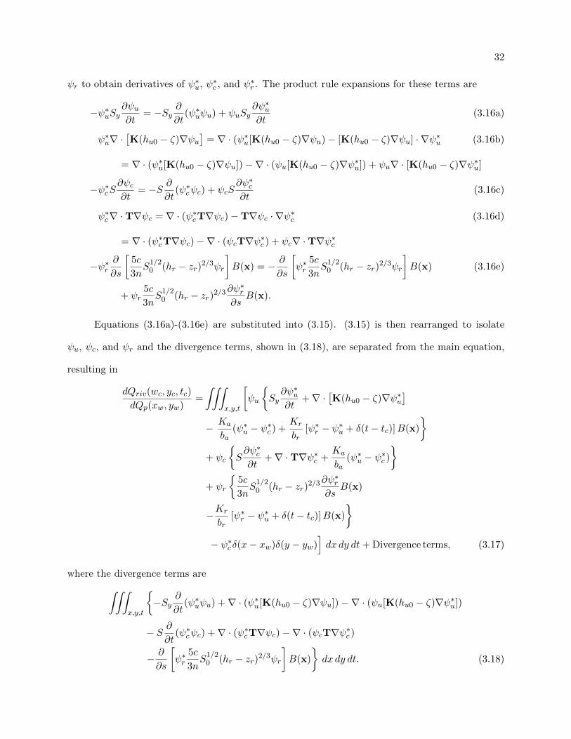
32

ψr to obtain derivatives of ψ∗u, ψ∗c , and ψ∗r . The product rule expansions for these terms are

−ψ∗uSy∂ψu∂t

= −Sy∂

∂t(ψ∗uψu) + ψuSy

∂ψ∗u∂t

(3.16a)

ψ∗u∇ ·[K(hu0 − ζ)∇ψu

]= ∇ · (ψ∗u[K(hu0 − ζ)∇ψu)− [K(hu0 − ζ)∇ψu] · ∇ψ∗u (3.16b)

= ∇ · (ψ∗u[K(hu0 − ζ)∇ψu])−∇ · (ψu[K(hu0 − ζ)∇ψ∗u]) + ψu∇ · [K(hu0 − ζ)∇ψ∗u]

−ψ∗cS∂ψc∂t

= −S ∂∂t

(ψ∗cψc) + ψcS∂ψ∗c∂t

(3.16c)

ψ∗c∇ ·T∇ψc = ∇ · (ψ∗cT∇ψc)−T∇ψc · ∇ψ∗c (3.16d)

= ∇ · (ψ∗cT∇ψc)−∇ · (ψcT∇ψ∗c ) + ψc∇ ·T∇ψ∗c

−ψ∗r∂

∂s

[5c

3nS

1/20 (hr − zr)2/3ψr

]B(x) = − ∂

∂s

[ψ∗r

5c

3nS

1/20 (hr − zr)2/3ψr

]B(x) (3.16e)

+ ψr5c

3nS

1/20 (hr − zr)2/3∂ψ

∗r

∂sB(x).

Equations (3.16a)-(3.16e) are substituted into (3.15). (3.15) is then rearranged to isolate

ψu, ψc, and ψr and the divergence terms, shown in (3.18), are separated from the main equation,

resulting in

dQriv(wc, yc, tc)

dQp(xw, yw)=

∫∫∫x,y,t

[ψu

Sy∂ψ∗u∂t

+∇ ·[K(hu0 − ζ)∇ψ∗u

]− Ka

ba(ψ∗u − ψ∗c ) +

Kr

br[ψ∗r − ψ∗u + δ(t− tc)]B(x)

+ ψc

S∂ψ∗c∂t

+∇ ·T∇ψ∗c +Ka

ba(ψ∗u − ψ∗c )

+ ψr

5c

3nS

1/20 (hr − zr)2/3∂ψ

∗r

∂sB(x)

−Kr

br[ψ∗r − ψ∗u + δ(t− tc)]B(x)

− ψ∗c δ(x− xw)δ(y − yw)

]dx dy dt+ Divergence terms, (3.17)

where the divergence terms are∫∫∫x,y,t

−Sy

∂

∂t(ψ∗uψu) +∇ · (ψ∗u[K(hu0 − ζ)∇ψu])−∇ · (ψu[K(hu0 − ζ)∇ψ∗u])

− S ∂∂t

(ψ∗cψc) +∇ · (ψ∗cT∇ψc)−∇ · (ψcT∇ψ∗c )

− ∂

∂s

[ψ∗r

5c

3nS

1/20 (hr − zr)2/3ψr

]B(x)

dx dy dt. (3.18)

33

The arbitrary functions ψ∗u, ψ∗c , and ψ∗r are now defined so that ψu, ψc, and ψr are eliminated

from (3.17), yielding

Sy∂ψ∗u∂τ

= ∇ ·[K(hu0 − ζ)∇ψ∗u

]− Ka

ba(ψ∗u − ψ∗c ) +

Kr

br[ψ∗r − ψ∗u + δ(τ)]B(x) (3.19a)

S∂ψ∗c∂τ

= ∇ ·T∇ψ∗c +Ka

ba(ψ∗u − ψ∗c ) (3.19b)

− 5c

3nS

1/20 (hr − zr)2/3∂ψ

∗r

∂s= −Kr

br[ψ∗r − ψ∗u + δ(τ)] (3.19c)

where τ = tc − t is backward time. To further simplify (3.17), the divergence terms are eliminated

by defining initial conditions and boundary conditions on ψ∗u, ψ∗c , and ψ∗r . The following initial and

boundary conditions cause the divergence terms to vanish:

ψ∗u = ψ∗c = 0 at y = 0 and y = Ly, (3.20a)

∇ψ∗u · ~n = ∇ψ∗c · ~n = 0 at x = 0 and x = Lx, (3.20b)

ψ∗r = 0 at s = Ls, (3.20c)

ψ∗u(x, τ = 0) = ψ∗c (x, τ = 0) = 0, . (3.20d)

The variables ψ∗u, ψ∗c , and ψ∗r are the adjoint states of hu, hc, and hr, and (3.19a), (3.19b), and

(3.19c) are the adjoints of (3.1a), (3.1b), and (3.9), respectively. The adjoint sensitivity equation

resulting from the above simplifications of (3.17) is evaluated at the compliance time, t = tc (τ = 0),

and at the compliance location, (xc, yc). After using (3.19a), (3.19b), and (3.19c) and the boundary

and initial conditions above, (3.17) reduces to

dQriv(xc, yc, τ = 0)

dQp(xw, yw)=

∫∫∫x,y,τ−ψ∗c δ(x− xw)δ(y − yw) dx dy dτ =

∫ tc

τ=0−ψ∗c (xw, yw, τ) dτ. (3.21)

Changing the variables (xw, yw) to (x, y), (3.21) is written as

dQriv(xc, yc, τ = 0)

dQp(x, y)=

∫ tc

τ=0−ψ∗c (x, y, τ) dτ. (3.22)

Stream depletion is found using (3.19a), (3.19b), and (3.19c) to solve for ψ∗c then integrating

over time as indicated in (3.22) and multiplying by the pumping rate. Solving this system of

equations provides stream depletion values for a well at any arbitrary location (x, y) in the confined

34

aquifer. The same approach can be used when pumping occurs in the unconfined aquifer, however,

the ψ∗c δ(x−xw)δ(y−yw) term will be absent in the confined aquifer equations and it will be replaced

by the term ψ∗uδ(x− xw)δ(y− yw) in the unconfined aquifer equations. The final adjoint equations

for pumping in the unconfined aquifer is

dQriv(xc, yc, τ = 0)

dQp(x, y)=

∫ tc

τ=0−ψ∗u(x, y, τ) dτ. (3.23)

The adjoint equations are solved to obtain ψ∗c and ψ∗u, then ψ∗c is used in (3.22) and ψ∗u is used

in (3.23) to find dQriv

dQpdue to pumping in the confined and unconfined aquifer, respectively, then

multiplying by the pumping rate to obtain stream depletion, expressed as

∆Qriv =dQrivdQp

Qp, (3.24)

where ∆Qriv is stream depletion.

3.6 MODFLOW Modifications

To eliminate the need to run many forward simulations to calculate stream depletion, we

adapt MODFLOW to solve equations (3.19a)-(3.19c), thus allowing us to model the stream deple-

tion more efficiently. This is done by modifying the input values into MODFLOW and modifying

the source code of the STR package.

3.6.1 Input Modifications

The adjoint equations, (3.19a), (3.19b), and (3.19c), have essentially the same form as the

forward governing equations, (3.1a), (3.1b), and (3.9), so MODFLOW can be used to solve the

adjoint equation. In the adjoint equations, the state variables are the adjoint states, ψ∗u, ψ∗c , and

ψ∗r , while in the forward equations the state variables are head. Thus when we use MODFLOW to

solve the adjoint equations, “head” is a surrogate for the adjoint state. The adjoint equations are

written in terms of τ , which is backwards time, so when we use MODFLOW to solves the adjoint

equations, time becomes backward time, τ .

35

One of the first issues that arises in running an adjoint simulation based on equations (3.19a)-

(3.19c) results from the initial condition in (3.20d), which indicates that ψ∗u = 0 and ψ∗c = 0 when

τ = 0 and would be entered into the MODFLOW input files as an initial condition of zero. In

MODFLOW, when the head in a model cell drops below the bottom elevation of the cell, the cell

“goes dry” and calculations are no longer performed on that cell. To avoid this, we define new state

variables with magnitudes greater than the aquifer bottom elevation. These new state variables

are defined as

Ψ∗u(x, τ) = β + ψ∗u(x, τ)/γ, (3.25a)

Ψ∗c(x, τ) = β + ψ∗c (x, τ)/γ, (3.25b)

Ψ∗r(x, τ) = β + ψ∗r (x, τ)/γ, (3.25c)

where β is defined so that it is higher than the bottom elevation of all the aquifers in the model

as well as the river bottom, yet lower than the land surface elevation. Setting the value of β to

be greater than the bottom elevation of the aquifer ensures cells will not go dry due to the initial

conditions. For a natural system, the value of β would be determined by finding the lowest point of

land surface elevation throughout the domain and checking to make sure this is above the elevation

of the bottom of the riverbed and the bottom elevation of the aquifer. The definition of γ is

described below.

These new state variables are substituted into (3.19a)-(3.19c), yielding

Sy∂Ψ∗u∂τ

= ∇ ·[K(hu0 − ζ)∇Ψ∗u

]− Ka

ba(Ψ∗u −Ψ∗c) +

Kr

br[Ψ∗r −Ψ∗u]B(x), (3.26a)

S∂Ψ∗c∂τ

= ∇ ·T∇Ψ∗c +Ka

ba(Ψ∗u −Ψ∗c), (3.26b)

− 5c

3nS

1/20 (hr − zr)2/3∂Ψ∗r

∂s= −Kr

br[Ψ∗r −Ψ∗u] , (3.26c)

36

with the following initial and boundary conditions:

Ψ∗u = Ψ∗c = β at y = 0 and y = Ly, (3.27a)

∇Ψ∗u · ~n = ∇Ψ∗c · ~n = 0 at x = 0 and x = Lx, (3.27b)

Ψ∗r = β at s = Ls, (3.27c)

Ψ∗u(x, τ = 0) = β +Kr

brSyγB(x), (3.27d)

Ψ∗c(x, τ = 0) = β. (3.27e)

The δ(τ) term in (3.19a) is now part of the initial condition in (3.27d). The δ(τ) term in (3.19c)

would be part of the initial condition on Ψ∗r ; however, the temporal changes in Ψ∗r are assumed to

occur more rapidly than the changes in aquifer head and they are neglected here.

The purpose of γ is to ensure that the second term in (3.27d) is of the same order of magnitude

as β. This second term is the load term to the adjoint simulation and represents an instantaneous

perturbation at the river that is propagated into the aquifer over time. If the magnitude of this

perturbation is too small, it will be on the same order of magnitude as the numerical error in the

model and will not be noticeable in the simulation results. We use γ 1 to prevent this. Using

(3.25a) and (3.25b) in (3.23) and (3.22), the adjoint sensitivity equations become:

dQriv(xc, yc, τ = 0)

dQp(x, y)=

∫ tc

τ=0γ [−Ψ∗u(x, y, τ)− β] dτ, (3.28a)

dQriv(xc, yc, τ = 0)

dQp(x, y)=

∫ tc

τ=0γ [−Ψ∗c(x, y, τ)− β] dτ. (3.28b)

Another issue arises when attempting to model the first term on the right-hand side of the

governing equation of groundwater flow (3.26a) in MODFLOW. The first term on the right-hand

side of (3.1a) is non-linear in the state variable, while the first term on the right-hand side of (3.26a),

the adjoint equation we want MODFLOW to solve, is linear in the adjoint state and depends on the

initial head in the unconfined aquifer. For MODFLOW to handle this term, the unconfined aquifer

is modeled as a confined aquifer with a transmissivity of T = K(hu0 − ζ). Doing so assumes that

the drawdown in the unconfined aquifer is small compared to the saturated thickness.

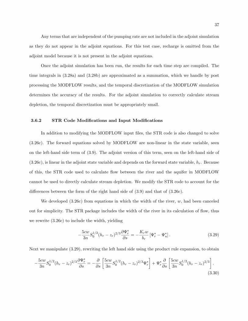
37

Any terms that are independent of the pumping rate are not included in the adjoint simulation

as they do not appear in the adjoint equations. For this test case, recharge is omitted from the

adjoint model because it is not present in the adjoint equations.

Once the adjoint simulation has been run, the results for each time step are compiled. The

time integrals in (3.28a) and (3.28b) are approximated as a summation, which we handle by post

processing the MODFLOW results, and the temporal discretization of the MODFLOW simulation

determines the accuracy of the results. For the adjoint simulation to correctly calculate stream

depletion, the temporal discretization must be appropriately small.

3.6.2 STR Code Modifications and Input Modifications

In addition to modifying the MODFLOW input files, the STR code is also changed to solve

(3.26c). The forward equations solved by MODFLOW are non-linear in the state variable, seen

on the left-hand side term of (3.9). The adjoint version of this term, seen on the left-hand side of

(3.26c), is linear in the adjoint state variable and depends on the forward state variable, hr. Because

of this, the STR code used to calculate flow between the river and the aquifer in MODFLOW

cannot be used to directly calculate stream depletion. We modify the STR code to account for the

differences between the form of the right hand side of (3.9) and that of (3.26c).

We developed (3.26c) from equations in which the width of the river, w, had been canceled

out for simplicity. The STR package includes the width of the river in its calculation of flow, thus

we rewrite (3.26c) to include the width, yielding

−5cw

3nS

1/20 (hr − zr)2/3∂Ψ∗r

∂s= −Krw

br[Ψ∗r −Ψ∗u] . (3.29)

Next we manipulate (3.29), rewriting the left hand side using the product rule expansion, to obtain

−5cw

3nS

1/20 (hr − zr)2/3∂Ψ∗r

∂s= − ∂

∂s

[5cw

3nS

1/20 (hr − zr)2/3Ψ∗r

]+ Ψ∗r

∂

∂s

[5cw

3nS

1/20 (hr − zr)2/3

].

(3.30)

38

Expanding the derivative of last term in (3.30) results in

Ψ∗r∂

∂s

[5cw

3nS

1/20 (hr − zr)2/3

]= Ψ∗r

5c

3

[− wn2S

1/20 (hr − zr)2/3∂n

∂s+w

2nS−1/20 (hr − zr)2/3∂S0

∂s

+2w

3nS

1/20 (hr − zr)−1/3∂(hr − zr)

∂s+

1

nS

1/20 (hr − zr)2/3∂w

∂s

].

(3.31)

Substituting (3.30) and (3.31) into (3.26c), we rewrite (3.26c) as

− ∂

∂s

[5cw

3nS

1/20 (hr − zr)2/3Ψ∗r

]+ Ψ∗r

5c

3

[− wn2S

1/20 (hr − zr)2/3∂n

∂s+w

2nS−1/20 (hr − zr)2/3∂S0

∂s

+2w

3nS

1/20 (hr − zr)−1/3∂(hr − zr)

∂s+

1

nS

1/20 (hr − zr)2/3∂w

∂s

]= −Krw

br[Ψ∗r −Ψ∗u] .

(3.32)

For comparison, the forward equation for the river mass balance, shown in (3.9), is repeated here,

with the river width included,

∂

∂s

[wcnS

1/20 (hr − zr)5/3

]= −Krw

br(hr − hu). (3.33)

This is the equation that is solved in the STR packages, thus, we modify the STR package to solve

(3.32) instead and call the modified version STRADJ.

The first term on the left-hand side of (3.32) is similar to the term on the left-hand side

of (3.33). The adjoint version is linear in the state variable, Ψ∗r , while the forward equation is

non-linear, so the code is changed to handle this difference along with the different constant for the

adjoint version. The presence of the forward river head, hr, in the adjoint version of the equation

must also be accounted for in the STRADJ code. To obtain results for hr, additional simulations

would need to be run for every cell in the model domain, thus eliminating any computational

advantage provided by the adjoint approach. We avoid this by using a constant value in place of

hr, which we call hrc. If hrc is set to the initial head in the river, the term (hr − zr)2/3 in the first

term of the left-hand side of (3.32) would represent no change in the river head due to depletion,

so the stream depletion values calculated in this case would likely be lower than actual values.

Another approach would be to set hrc according the river level associated with some maximum

39

depletion, for instance, the stream depletion that defines non-tributary groundwater discussed in

Section 1.3.5. The calculated stream depletion values in this case would likely be higher than the

actual values. Because hrc does not exist in the STR code, it is added into the STRADJ input file

and the (hr − zr)2/3 term accounted for in the STRADJ code.

The second term on the left-hand side of (3.32) does not exist in (3.33) and is added to the

STRADJ code. In order for the STRADJ code to calculate the derivatives with respect to s in

this term, the length of each reach must be specified to calculate ds. In the STR package, reach

length is lumped together with other parameters in the streambed hydraulic conductance term.

For STRADJ, the reach length is added to the STRADJ input file to aid in the code’s execution.

The order in which the STRADJ code is changed to account for the river flow being reversed

in the adjoint simulation. For the forward model, calculations begin in the first reach, which is the

upstream-most reach, and proceed in a downstream manner. The STRADJ is modified to perform

calculations in the reverse order, beginning at the downstream-most reach and working upstream.

The boundary conditions must be modified because the river flow is reversed in the adjoint

simulation and the order of calculations of the STRADJ code is reversed. For the forward model,

the boundary condition in the river is handled by the STR package as an inflow that corresponds

to head in the farthest upstream reach and enters at the uppermost reach in the model. Recall

from (3.27c) that the adjoint version of the river mass balance has its boundary on the lowest reach

in the system because the adjoint equations begin at Ls, the downstream end of the river. The

STRADJ code is modified so that the boundary condition enters at the lowest reach in the model.

The value of this boundary condition, which is a surrogate for inflow, is calculated from the first

term of the right hand side of (3.32) as

Φ =5cw

3nS

1/20 (hrc − zr)2/3Dadj , (3.34)

where Φ is the surrogate for inflow and Dadj = Ψ∗r − zr is the surrogate for river depth. The value

of Φ is entered in the STRADJ input file as flow for the last reach in the model, and the value of

the flow for the first reach in the model is set to zero.

40

The STRADJ code can be found in Appendix A. For reference, Table 3.1 shows a list of the

variables used for the STR and STRADJ package input file, the corresponding variable in the STR

package code, and the corresponding variable used in our notation throughout this work.

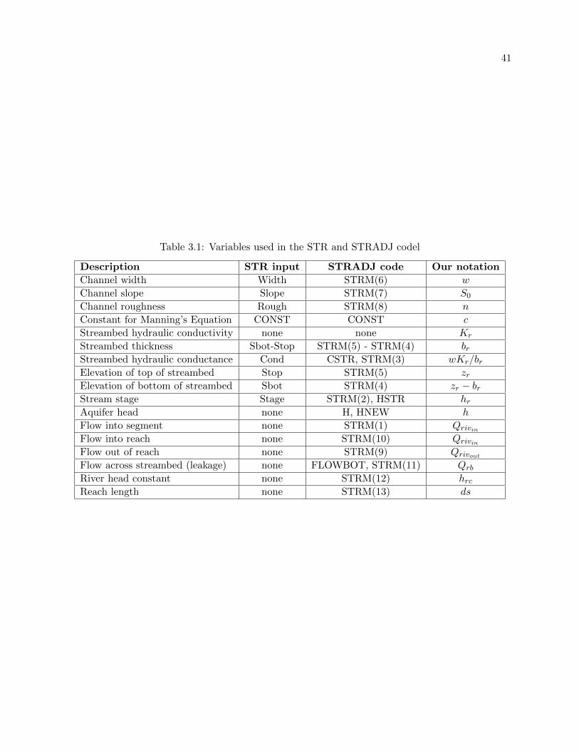
41

Table 3.1: Variables used in the STR and STRADJ codel

Description STR input STRADJ code Our notation

Channel width Width STRM(6) w

Channel slope Slope STRM(7) S0

Channel roughness Rough STRM(8) n

Constant for Manning’s Equation CONST CONST c

Streambed hydraulic conductivity none none Kr

Streambed thickness Sbot-Stop STRM(5) - STRM(4) brStreambed hydraulic conductance Cond CSTR, STRM(3) wKr/brElevation of top of streambed Stop STRM(5) zrElevation of bottom of streambed Sbot STRM(4) zr − brStream stage Stage STRM(2), HSTR hrAquifer head none H, HNEW h

Flow into segment none STRM(1) QrivinFlow into reach none STRM(10) QrivinFlow out of reach none STRM(9) QrivoutFlow across streambed (leakage) none FLOWBOT, STRM(11) QrbRiver head constant none STRM(12) hrcReach length none STRM(13) ds

Chapter 4

Test Case

In order to verify the adjoint methodology developed in the previous chapter, we run a test

case using MODFLOW to compare the stream depletion results calculated using the standard

forward approach to those found with the adjoint method. We show the results from the forward

test case in Section 4.2 and compare these with the results from the adjoint test case in Section

4.3.

4.1 Conceptual Model

We develop a model for the test case based on the hypothetical aquifer described in Section

3.1 and shown in Figure 3.1. It has two 20 m thick layers, an unconfined aquifer on top and a

confined aquifer on bottom, with a simulated confining layer between them. The model domain

spans from x = 0 m to x = Lx = 1600 m in the x-direction and from y = 0 m to y = Ly = 2000

m in the y-direction. No flow boundary conditions exist at x = 0 m and x = 1600 m and constant

head boundary conditions of h = 10 m and h = 9 m exist at y = 0 m and y = Ly = 2000 m,

respectively. The model discretization is ∆x = 50 m by ∆y = 50 m, yielding 40 rows and 32

columns. We employ the Dupuit assumptions in the unconfined aquifer and assume the flow in the

confined aquifer is essentially horizontal as well. Additionally, we assume both the confined and

unconfined aquifers are isotropic. A meandering river flows from y = Ly to y = 0 m and penetrates

10 m into the unconfined aquifer, with a path defined by the equation

xcl = 775 m + 250 m sin

(2π

y − dy/2ymax − dy

), (4.1)

43

where xcl is the x coordinate of the centerline of the river, dy = 50 m is the spatial discretization

in the y−direction, and ymax = 2000 m is the length of the model domain in the y−direction. A

pumping well can extract water from either the confined or unconfined aquifer at a rate of Qp = 10

m3/d.

We use MODFLOW to simulate the model, with the river modeled using the STR package,

pumping wells modeled using the well (WEL) package, and recharge modeled with the recharge

(RCH) package. The model also employs the preconditioned partial-gradient (PCG) package and

block-centered flow (BCF) packages to solve the finite difference equations. Table 4.1 lists the

values used to construct the model.

4.2 Forward Simulations

For the standard forward model, calculating stream depletion for each potential well location

in the hypothetical aquifer system requires an initial model run to determine the flow rate across

the riverbed in the absence of pumping. Next, a separate model run finds the flow rate across the

riverbed as a result of pumping in the cell located in the first row and column of the unconfined

aquifer. The difference in flow rates across the riverbed between the initial simulation and the

simulation with pumping is calculated and saved. Additional simulations are run to cycle the

pumping well through each cell of the model domain, with a separate simulation required for each

cell and the difference in flow rates saved for each simulation. The stream depletion for each

possible well location is shown in Figure 4.1 c,d. Figure 4.1 c,d shows higher stream depletion

values for wells located near the river and lower values for wells further from the river. The low

stream depletion values near y = Ly and y = 0 m are caused by the constant head boundaries at

y = Ly and y = 0 m. A well located near these boundaries will draw all of its water from the

fixed head boundary rather than from the aquifer in the model domain and the river. For our

hypothetical aquifer, a total of 2560 simulations are needed in addition to the initial simulation to

determine stream depletion for a well located at the center of every grid block in the model domain.

The runtime required to perform all simulation runs and compile the results is 4 hours 36 minutes

44

Table 4.1: Forward aquifer and model parameters.

Description Value

Head at north boundary, hu(x, t) and hc(x, t) at y = 2000 m 20 m

Head at south boundary, hu(x, t) and hc(x, t) at y = 0 m 16 m

Elevation of bottom of confined aquifer -20 m

Elevation of top of confined aquifer -10 m

Elevation of bottom of unconfined aquifer, ζ 0 m

Hydraulic conductivity of unconfined aquifer, K 0.2 m/d

Hydraulic conductivity of aquitard, Ka 0.02 m/d

Transmissivity of confined aquifer, T 1.0 m2/d

Specific yield, Sy 0.2

Storage coefficient in aquitard 0

Storage coefficient in confined aquifer, S 1×10−3

Recharge rate, N 4×10−7 m/d

River bottom elevation, zr 15.125 m

Riverbed thickness, br 0.125 m

River width, w 25 m

Hydraulic conductivity of the riverbed, Kr 2.5×10−5 m/d

Manning’s coefficient of roughness for the riverbed, n 0.04

Riverbed slope, S0 0.001

Spatial discretization 50 × 50 m

Temporal discretization 1 d

Compliance time, tc 1825 d

Pumping rate, Qw 10 m3/d

Initial head in unconfined aquifer, hu0(x) 16 m

Initial head in confined aquifer, hc0(x) 16 m

Initial river stage, hr 19 m

River flow, Qr0 16,325,000 m3/d

45

(16,560 seconds) on a HP Workstation XW4100 with a Dual core 2.4 GHz processor and 1.5 Gb of

RAM.

4.3 Adjoint Simulation

Using the modifications to MODFLOW described in Sections 3.6.1 and 3.6.2, we run an ad-

joint simulation based on the same hypothetical aquifer with a partially penetration meandering

stream used in the forward simulation. Several of the same MODFLOW input files are used to

run the adjoint simulation; however, some of them are modified. These include the basic (BAS),

discretization (DIS), and block centered flow (BCF) package files. The MODFLOW code is recom-

piled to include the STRADJ version of the STR package in place of the regular STR package and

the inputs to the STR package are also modified. The well (WEL) package and recharge (RCH)

package are not used in the adjoint simulation.

The basic package file is modified from the forward model by setting the initial head through-

out the unconfined and confined aquifer to β = 16. Additionally, the model cells directly below

the river in the unconfined aquifer are set to according to the initial condition shown in (3.27d).

To account for cases where the river doesn’t occupy an entire cell, this initial condition is slightly

modified by dividing the area of the river by the area of the cell, and this term is used to replace

the B(x) term in (3.27d), resulting in

Ψ∗u(x, τ = 0) = β +Kr

brSyγ

ArivAtot

, (4.2)

where Ariv is the area of the river in a model cell and Atot is the area of of the cell the river passes

through.

The block centered flow package file is changed so that the unconfined aquifer is modeled as

a confined aquifer with a primary storage coefficient of Sy and a transmissivity of T = K(hr0− ζ).

The STR package input file is modified by setting the initial flow in the furthest upstream

reach to zero and setting the initial flow in the furthest downstream reach to Φ. The additional

inputs, the river head constant hrc and the reach length ds, are added to the input file for each

46

Figure 4.1: Stream depletion (m3/d) from forward and adjoint simulations (a) Adjoint results withpumping in the unconfined aquifer. (b) Adjoint results with pumping in the confined aquifer. (c)Forward results with pumping in the unconfined aquifer. (d) Forward results with pumping in theconfined aquifer.

47

Table 4.2: Adjoint aquifer and model parameters.

Description Value

ψ∗u(x, τ) and ψ∗c (x, τ) at north and south boundary, y = 2000 m and y = 0 m 16 d−1

β 16 d−1

γ 1×10−5

Initial adjoint state in unconfined aquifer, ψ∗u(x, τ = 0) β + KrbrSyγ

B(x)

Initial adjoint state in lower confined aquifer, ψ∗c (x, τ = 0) 16 d−1

Adjoint “river flow”, Φ 6,143,724 m3/d

River head constant, hrc 19 m

reach of the river. For this simulation, the river head constant, hrc, is set to 19 m, representing a

scenario with minimum depletion.

Table 4.2 lists the values used to construct the adjoint model. If a parameter is not listed it

has not changed from the forward model.

Only one adjoint simulation is required to obtain stream depletion values that correspond

to a pumping well located anywhere in the model domain. Equations (3.26a)-(3.26c) are solved in

MODFLOW and the results are used in (3.28a), (3.28b) and (3.24) to calculate stream depletion

based on a pumping rate of Qp=10 m3/d. Figure 4.1 a,b shows the adjoint stream depletion results

above the forward results for both unconfined and confined aquifers. As with the forward simulation,

the stream depletion is higher for a pumping well located near the river and the depletion is lower

the further from the river the pumping well is located. The results of the adjoint simulations

are visually indistinguishable from forward simulation results, indicating the adjoint methodology

accurately calculates stream depletion.

The runtime required to complete the MODFLOW adjoint simulation was 22.9 seconds on a

HP Workstation XW4100 with a Dual core 2.4 GHz processor and 1.5 Gb of RAM, and the required

time to post process the results was 29 seconds, resulting in a total time required to calculate the

adjoint stream depletion of 52 seconds. This is three orders of magnitude less than the computation

time required to run the forward simulations. Clearly, the adjoint method provides a much more

efficient approach to quantifying stream depletion.

48

The error between the forward and adjoint simulation varied spatially, with the error near

the river greater than the error further from the river. The spatial behavior of the absolute error,

calculated as the adjoint stream depletion minus the forward stream depletion, is shown in Figure

4.2. The adjoint results are higher than those of the forward simulations for the majority of the

domain, with the exception of a few cells that lie directly below the river in the unconfined aquifer.

The maximum absolute error in the unconfined aquifer is 0.0116 m3/d and occurs in row 35, y=300

m, and column 10, x=500 m, of the domain, while the maximum absolute error for the confined

aquifer is 0.0102 m3/d and occurs at row 23, y=900 m, and column 19, x=950 m, of the domain.

The relative error at these two locations is 2.14% and 2.34% for the unconfined and confined

aquifer, respectively. The relative error is lowest near the river and increases as the location of the

pumping well moves away from the river, as seen in Figure 4.3. The behavior of the relative error

becomes erratic in locations further away from the river where the values of the forward stream

depletion approach zero. In these location, the absolute error is divided by infinitesimally small

values of the forward stream depletion. The relative error in the unconfined aquifer is also negative

in the cells underlying the river, shown in white in Figure 4.3. In areas where the depletion values

are above 0.1 m3/d, the relative error is less than 10%. On the whole, the adjoint results are

relatively accurate, especially considering the assumptions made to solve the adjoint equation that

theoretically depends on the forward model results.

49

Figure 4.2: Absolute error between the adjoint and forward simulations calculated as the adjointstream depletion minus the forward stream depletion for (a) the unconfined aquifer and (b) theconfined aqufier.

Figure 4.3: Relative error between the adjoint and forward simulations for the unconfined aquifer,(a), and the confined aquifer, (b).

Chapter 5

Discussion

The results of the forward and adjoint simulations show the adjoint methodology works well

and provides a great deal of stream depletion information with much less computational expense.

In this chapter, we investigate the assumptions of the approach and the limitations of this method.

5.1 Assumptions

In developing the forward and adjoint models, we make several common assumptions about

the behavior of groundwater flow in the model domain and the geometry of the river as well as

assumptions that simplify our calculations. We employ the Dupuit assumption, which assumes

groundwater flows horizontally in unconfined aquifers, and we also assume flow is horizontal in the

confined aquifer.

One assumption we make is that drawdown in the unconfined aquifer is small compared to

aquifer thickness. We approximate the saturated thickness in the unconfined aquifer, (hu − ζ),

using the initial head as (hu0 − ζ), as seen in (3.12a). To test this assumption, we compared the

heads in the unconfined aquifer before and after pumping using a pumping well located away from

the model boundaries and from the river, all of which might cause less drawdown. When pumping

from the unconfined aquifer at the location (x, y)=(400 m, 1000 m) at a pumping rate of Qp =

10 m3/d, the largest difference between the initial head in the aquifer and the head after pumping

for 5 years (1825 days) occurs at the pumping location, as seen in Figure 5.1. This difference at

the pumping well is 1.377 m, which is 6.89% of the 20 m thickness of the unconfined aquifer. This

51

Figure 5.1: Head (m) in the model domain when pumping occurs in the unconfined aquifer at(x, y)=(400 m, 1000 m). Thick contour lines represent head in the unconfined aquifer and thincontour lines represent head in the confined aquifer.

52

maximum drawdown only impacts the model heads in the vicinity of the pumping well with an

area with a radius of about 200 m from the well. The average difference between initial heads and

heads after pumping across the unconfined aquifer is 0.023 m, which is 0.11% of the 20 m thickness

of the unconfined aquifer. While drawdown in the immediate vicinity of the well might cause some

vertical flow, the average drawdown is several orders of magnitude less than the aquifer thickness,

indicating the assumption that drawdown in the unconfined aquifer is small compared to the aquifer

thickness appropriately represents the behavior of the head. Cases where this assumption might

not hold true include instances when the pumping rate is very high, causing higher depletions,

especially in the vicinity of the pumping well, or in case where the unconfined aquifer is not very

thick compared to the drawdown.

To test our assumption that the stream depletion will scale linearly with the pumping rate,

we run several forward simulations using different pumping rates. We use a pumping well located

at (x, y)=(400 m, 1000 m), and stream depletion was calculated using the forward approach in

the same manner described in Section 4.2. The range of pumping rates we use is limited by the

numerical precision of the model and the thickness of the unconfined aquifer. If the pumping rate

is too low, the stream depletion will be on the same order as the model precision and it will appear

there is no stream depletion. If the pumping rate is too high, the head in the cell containing the

pumping well will drop below the bottom elevation of the unconfined aquifer, causing the cell to

go dry and no longer be included in model calculations, resulting in the model calculating stream

depletion inaccurately. For our model, the range of pumping rates that provide meaningful stream

depletion results are 2 m3/d ≤ Qp ≥ 62 m3/d. Figure 5.2 shows the forward stream depletion

plotted over this range of pumping rates. The behavior of the stream depletion is linear, indicating

that this assumption is correct.

We also assume that using a value 19 m for hrc in the adjoint simulation will not underestimate

the forward values for stream depletion. After completing the adjoint simulation, we ran additional

adjoint simulations with different values of hrc to test how sensitive the adjoint stream depletion

results were to hrc and found no difference in depletion between hrc = 18 m, a river head constant

53

Figure 5.2: Linear scaling of forward stream depletion with puming rate.

54

Figure 5.3: An aquifer underlying a slope where a single value of β does not remain above theelevation of the bottom of the aquifer and the river and below the land surface elevation.

representing high depletion, and hrc = 19 m. We also found the difference in depletion between

hrc = 15.25 m, a river head constant representing a case where the river has almost run dry, and

hrc = 19 m was less than 2×10−7 m. From these results we conclude that a river head constant of

hrc = 19 m does not cause the adjoint depletion to underestimate the actual depletion.

5.2 Limitations

While this work provides an efficient method for determining stream depletion resulting from

a new well at an unspecified location, it does have a few limitations. One of the main limitations

lies in the bounds on the parameter β. Recall that β is used to prevent cells from going dry in

the adjoint simulation and must be greater than the elevation of the bottom of the aquifer and the

bottom of the riverbed but below the land surface elevation. These bounds are easily met if an

aquifer and the overlying land surface are fairly flat; however, if an aquifer underlies a steep slope

the bounds on β may not be able to be met throughout the model domain. Figure 5.3 represents a

case where no single value of β can be used throughout the aquifer and this method of determining

stream depletion can not be used to find stream depletion in this domain.

Another limitation of this method is that it cannot be used to to site multiple wells based on

55

the the lowest possible stream depletion. Several cases where more than one well might be desired

or required exist, such as required emergency wells or well fields that employ several wells; however,

this work develops adjoint equation based on a single pumping well.

This method is also limited by its inability to handle situations where aquifer head drops below

the river bottom the aquifer is no longer hydraulically connected to the river. In this instance, no

additional stream depletion will occur. The adjoint method is not simulating head; it simulates the

adjoint state and is not able to determine if the aquifer head drops below the river bottom. If the

head does drop below the aquifer bottom, the adjoint method will continue calculating depletion

that is not physically occurring and will over predict stream depletion, making it a conservative

estimate. To avoid this, forward simulations can be run at selected locations with high depletion

afterwards to determine if the aquifer has become disconnected from the river.

This work also assumes the river can be approximated as a wide rectangular channel where

the width is much greater than the depth, allowing us to simplify Manning’s equation. Most

rivers and streams have different channel geometries and may not be well represented by a wide

rectangular channel.

The revised STRADJ code is not currently set up to handle named parameters or diver-

sions. This in not a limitation of the adjoint methodology, it is simply a limitation of the current

implementation and will be addressed in future work.

Chapter 6

Conclusion & Future Work

In this final chapter, we present our conclusions and discuss areas of future work for the

adjoint method of quantifying stream depletion.

6.1 Conclusions

This work develops an adjoint method for finding stream depletion caused by pumping in

an aquifer that is hydraulically connected to a river using the adjoint approach. With only one

simulation, the adjoint method provides the stream depletion associated with a pumping well

located anywhere in the model domain. This information is useful for identifying locations for new

wells that minimize stream depletion or for understanding what areas along a river section are most

sensitive to pumping.

The adjoint method we develop in this work accurately approximates the stream depletion

values for simulations that adhere to the assumptions we use to develop the adjoint approach. For

a test case using a hypothetical aquifer, the adjoint stream depletion values are visually indistin-

guishable from the forward stream depletion values. The relative error between the adjoint and

forward simulations is small.

The adjoint simulation proved to be far more computationally efficient than the forward

simulations. Adjoint stream depletions for the model domain were found in 52 seconds, while the

stream depletions results for the forward model took 4 hours and 36 minutes. The adjoint approach

provides an accurate approximation of stream depletion in several orders of magnitude less time.

57

6.2 Future Work

This works proves the value of an adjoint approach to quantifying stream depletion and it

also highlights areas of future work. While the method has proved effective when applied to a

hypothetical aquifer, a case study comparing the adjoint stream depletion found using the method

described in this work to the stream found from a model of an actual aquifer will providing insight

into how the method works in a more complex model. A case study we intend to investigate is the

model of the Upper San Pedro Basin in southern Arizona and northern Mexico that was developed

by the USGS (Leake 2010).

In our development of the adjoint method, we did not investigate how the adjoint method

behaves when used in conjunction with other sources or sinks, such as evapotranspiration. Addi-

tional work developing the adjoint method to accommodate additional sources and sinks that exist

in natural systems will further the applicability of this work.

Another area of future work lies in Type III boundary conditions. Neupauer and Griebling

(2011) developed the adjoint theory for Type III boundary conditions of the form αh+ β∆h · n =

g3(t). This theory needs to be tested with the coupled version of the adjoint equations presented

in this work.

Many of the limitations listed in Section 5.2 can be addressed by developing an adjoint version

of the SFR package. The STR package is not designed to calculate unsaturated flow between the

aquifer and the riverbed; however the stream flow routing (SFR) package has the capability of

modeling unsaturated zone flow (Niswogner and Prudic 2005). To find stream depletion for cases

where the aquifer head drops below the riverbed and unsaturated flow occurs, adjoint equations for

unsaturated zone flow must be developed along with an adjoint version of the SFR package designed

to handle these equations. The SFR package is also able to handle multiple channel geometries

based on an eight point cross section, so the adjoint equations can be modified to account for an

eight point point channel geometry and the SFR package modified to calculate these equations

(Prudic et al. 2004). Another capability of the SFR package is an alternate approach to calculating

58

stream depth and width from depth-discharge and width-discharge functions based on streamflow

gage regressions. An adjoint version of the regression equations could be developed in place of the

depth to flow relationship based on Manning’s equation used in this work.

Another area of future work involves adapting this work to handle situations where stream

depletion information is desired in systems with multiple wells. One approach to handling multiples

wells is an optimization method that identifies a well configuration that minimized stream depletion.

References

Ahlfeld, D., J. Mulvey, G. Pinder, and E. Wood (1988, MAR). Contaminated Groundwater Remedi-ation Design Using Simulation, Optimization, and Sensitivity Theory. 1. Model Development.Water Resources Research 24(3), 431–441.

Bernstien, L. (2008). Climate change 2007: synthesis report.Interngovernmental Panel on Climate Change 1(1), 30–73.

Brookshire, D., H. Burness, J. Chermak, and K. Krause (2002). Western urban water demand.Natural resources journal 42, 873–898.

Butler, J., X. Zhan, and V. Zlotnik (2008, JUL-AUG). Pumping-induced drawdown and streamdepletion in a leaky aquifer system. GROUND WATER 46(4), 529–U3.

Butler, J., V. Zlotnik, and M. Tsou (2001, SEP-OCT). Drawdown and stream depletion producedby pumping in the vicinity of a partially penetrating stream. Ground Water 39(5), 651–659.

Cardiff, M. and P. Kitanidis (2008, NOV). Efficient solution of nonlinear, underdetermined inverseproblems with a generalized PDE model. COMPUTERS & GEOSCIENCES 34(11), 1480–1491.

Chen, X. and L. Shu (2002, MAY-JUN). Stream-aquifer interactions: Evaluation of depletionvolume and residual effects from ground water pumping. GROUND WATER 40(3), 284–290.

Chen, X. and Y. Yin (1999). Evaluation of streamflow depletion for vertical anisotropic aquifer.Journal of Environmental Systems 27(1), 55–70.

Chen, X. and Y. Yin (2001a). Streamflow depletion: modeling of reduced baseflow and inducedstream infiltration from seasonally pumped wells. JAWRA Journal of the American WaterResources Association 37(1), 185–195.

Chen, X. and Y. Yin (2001b). Streamflow depletion: modeling of reduced baseflow and inducedstream infiltration from seasonally pumped wells. JAWRA Journal of the American WaterResources Association 37(1), 185–195.

Cirpka, O. and P. Kitanidis (2000, OCT). Sensitivity of temporal moments calcu-lated by the adjoint-state method and joint inversing of head and tracer data.ADVANCES IN WATER RESOURCES 24(1), 89–103.

Di Matteo, L. and W. Dragoni (2005, MAR-APR). Empirical relationships for estimating streamdepletion by a well pumping near a gaining stream. GROUND WATER 43(2), 242–249.

Fienen, M., T. Clemo, and P. Kitanidis (2008, JUL 25). An interactive Bayesian geostatisticalinverse protocol for hydraulic tomography. WATER RESOURCES RESEARCH 44, .

Glover, R. and G. Balmer (1954, JUN). River depletion resulting from pumping a well near a river.TRANSACTIONS-AMERICAN GEOPHYSICAL UNION 35(Part 3), 468–470.

Hantush, M. (1965). Wells near streams with semipervious beds.JOURNAL OF GEOPHYSICAL RESEARCH 70(12), 2829–&.

60

Hunt, B. (1999, JAN-FEB). Unsteady stream depletion from ground water pumping.GROUND WATER 37(1), 98–102.

Hunt, B. (2003, JAN-FEB). Unsteady stream depletion when pumping from semiconfined aquifer.JOURNAL OF HYDROLOGIC ENGINEERING 8(1), 12–19.

Hunt, B. (2009, SEP). Stream Depletion in a Two-Layer Leaky Aquifer System.JOURNAL OF HYDROLOGIC ENGINEERING 14(9), 895–903.

Jyrkama, M. and J. Sykes (2006, JAN 19). Sensitivity and uncertainty analysis of the rechargeboundary condition. WATER RESOURCES RESEARCH 42(1), .

Kenny, J., N. Barber, S. Hutson, K. Linsey, J. Lovelace, and M. Maupin (2009). Estimated Useof Water in the United States in 2005: U.S. Geological Survey Circular 1344. United StateGeological Survey.

Lavenue, A. and J. Pickens (1992, JUN). Application of a coupled adjoint sensitivity and krigingapproach to calibrate a groundwater-flow model. WATER RESOURCES RESEARCH 28(6),1543–1569.

Leake, S., H. Reeves, and J. Dickinson (2010, SEP-OCT). A New Capture Fraction Method toMap How Pumpage Affects Surface Water Flow. GROUND WATER 48(5), 690–700.

Li, B. and T. Yeh (1998, MAY 20). Sensitivity and moment analyses of head in variably saturatedregimes. ADVANCES IN WATER RESOURCES 21(6), 477–485.

LU, A., F. Schmittroth, and W. Yeh (1988, MAY). Sequential estimation of aquifer parameters.WATER RESOURCES RESEARCH 24(5), 670–682.

McDonald, M. and A. Harbaugh (1988). A modular three-dimensional finite-differenceground-water flow model: Techniques of Water-Resources Investigations of the United StatesGeological Survey, Book 6. United State Geological Survey.

Michalak, A. and P. Kitanidis (2004, AUG 6). Estimation of historical groundwater contami-nant distribution using the adjoint state method applied to geostatistical inverse modeling.WATER RESOURCES RESEARCH 40(8), .

Neuman, S., G. Fogg, and E. Jacomson (1980). A Sttistical approach to the inverse problem ofaquifer hydrology. 2. Case-study. WATER RESOURCES RESEARCH 16(1), 33–58.

Neupauer, R. and G. SA (2012). Adjoint simulation of stream depletion due to aquifer pumping.Ground Water 50(1), 133–143.

Neupauer, R. and J. Wilson (1999, NOV). Adjoint method for obtaining backward-in-time location and travel time probabilities of a conservative groundwater contaminant.WATER RESOURCES RESEARCH 35(11), 3389–3398.

Neupauer, R. and J. Wilson (2001, JUN). Adjoint-derived location and travel time probabilities fora multidimensional groundwater system. WATER RESOURCES RESEARCH 37(6), 1657–1668.

Niswonger, R. and D. Prudic (2005). Documentation of the Streamflow-Routing (SFR2) Package toinclude unsaturated flow beneath streams–A modification to SFR1: U.S. Geological SurveyTechniques and Methods, Book 6. United State Geological Survey.

Prudic, D. (1989). Documentation of a computer program to simulate stream-aquifer relationsusing a modular, finite-difference, ground-water flow model: U.S. Geological Survey Open-FileReport 88-729. United State Geological Survey.

Prudic, D., L. Konikow, and E. Banta (2004). A new streamflow-routing (SFR1) package to simulatestream-aquifer interaction with MODFLOW-2000: U.S. Geological Survey Open-File Report2004-1042. United State Geological Survey.

Skaggs, T. and D. Barry (1996, AUG). Sensitivity methods for time-continuous, spatially discrete

61

groundwater contaminant transport models. WATER RESOURCES RESEARCH 32(8),2409–2420.

Sophocleous, M., A. Koussis, J. Martin, and S. Perkins (1995, JUL-AUG). Evaluation of simplifiedstream-aquifer depletion models for water rights administration. GROUND WATER 33(4),579–588.

Spalding, C. and R. Khaleel (1991, APR). An Evaluation of analytical solutions to estimatedrawdowns and stream depletions by wells. WATER RESOURCES RESEARCH 27(4), 597–609.

Statutes, C. R. (2010). Section 37, Article 90, Underground Water.Sun, D. and H. Zhan (2007, APR). Pumping induced depletion from two streams.

ADVANCES IN WATER RESOURCES 30(4), 1016–1026.Sun, N. and W. Yeh (1985). Identification of parameter structure in groundwater inverse problem.

WATER RESOURCES RESEARCH 21(6), 869–883.Sykes, J., J. Wilson, and R. Andrews (1985). Sensitivity analysis for sensitivity analysis for stready-

state groundwater flow using adjoint operations. WATER RESOURCES RESEARCH 21(3),359–371.

Tan, C., C. Tung, C. Chen, and W. Yeh (2008, MAR). An integrated opti-mization algorithm for parameter structure identification in groundwater modeling.ADVANCES IN WATER RESOURCES 31(3), 545–560.

Tarlock, D., J. Corbridge, D. Getches, and R. Benson (2009). Water Resource Management.Thompson Reuters.

Theis, C. (1935, AUG). The relation between the lowering of the piezometric sur-face and the rate and duration of discharge of a well using ground water storage.TRANSACTIONS-AMERICAN GEOPHYSICAL UNION 16(Part 2), 519–524.

Theis, C. (1941, AUG). The effect of a well on the flow of a nearby stream.TRANSACTIONS-AMERICAN GEOPHYSICAL UNION 22(Part 3), 734–738.

Townley, L. and J. Wilson (1985). Computationally efficient algorithms for parame-ter estimation and uncertainty propagation in numerical models of groundwater flow.WATER RESOURCES RESEARCH 21(12), 1851–1860.

v. Colorado, K. (1995). 514 U.S. 673, 115 S.Ct. 1733, 131 L.Ed.2d 759.Vemuri, V. and W. Karplus (1969). Identification of nonlinear paramters of ground water basins

by hybrid computation. WATER RESOURCES RESEARCH 5(1), 172–185.Wilson, J. and D. Metcalfe (1985). Illustration and verification of adjoint sensitivity theory for

steady-state gorundwater flow. WATER RESOURCES RESEARCH 21(11), 1602–1610.Wu, S., Y. Tan, C. Chen, S. Lin, and K. Ke (2008, DEC 30). A two-dimensional inverse model

to identify transmissivity in an anisotropic aquifer. HYDROLOGICAL PROCESSES 22(26),5086–5096.

Yeh, H., Y. Chang, and V. Mow (2008, FEB 1). Stream depletion rate and volume from groundwaterpumping in wedge-shape aquifers. JOURNAL OF HYDROLOGY 349(3-4), 501–511.

Yeh, T. and J. Zhang (1996, SEP). A geostatistical inverse method for variably saturated flow inthe vadose zone. WATER RESOURCES RESEARCH 32(9), 2757–2766.

YEH, W. and N. SUN (1990, SEP). Variational sensitivity analysis, datarequirements, and parameter-identification in a leaky aquifer system.WATER RESOURCES RESEARCH 26(9), 1927–1938.

Zlotnik, V. (2004a, JUN 24). A concept of maximum stream depletion rate for leaky aquifers inalluvial valleys. WATER RESOURCES RESEARCH 40(6), .

62

Zlotnik, V. (2004b, SEP 16). A concept of maximum stream depletion rate for leaky aquifers inalluvial valleys. WATER RESOURCES RESEARCH 40(9), .

Zlotnik, V. and H. Huang (1999, JUL-AUG). Effect of shallow penetration and streambed sedimentson aquifer response to stream stage fluctuations (analytical model). GROUND WATER 37(4),599–605.

Zlotnik, V. and D. Tartakovsky (2008, FEB). Stream depletion by groundwater pumping in leakyaquifers. JOURNAL OF HYDROLOGIC ENGINEERING 13(2), 43–50.

Appendix A

Adjoint Version of STR Code

Below is the modified version of the STR package code, which we call STRADJ, written in

fortran.

C! Time of File Save by ERB: 3/9/2006 5:28PM

C Last change: ERB 12 Sep 2002 4:49 pm

C ADJOINT VERSION of STR CODE

C MODIFIED by SAG

C MODIFIED by RMN, 3/17/2012, ADJOINT TRIBUTARY CALCULATIONS

SUBROUTINE GWF1STR6ALP(ISUM,ISUMI,LCSTRM,ICSTRM,MXSTRM,NSTREM,IN,

1 IOUT,ISTCB1,ISTCB2,NSS,NTRIB,NDIV,ICALC,CONST,

2 LCTBAR,LCTRIB,LCIVAR,LCFGAR,NPSTR,ISTRPB)

C

C-----VERSION 15APRIL1998 GWF1STR6ALP

C-----VERSION 12MAR1999 -- modified to use character strings longer

C-----than 4 characters and to change VBVL and VBNM DIMENSION to MSUM

C ******************************************************************

C ALLOCATE ARRAY STORAGE FOR STREAMS

C ******************************************************************

C

C SPECIFICATIONS:

C ------------------------------------------------------------------

CHARACTER*200 LINE

C ------------------------------------------------------------------

C

C1------IDENTIFY PACKAGE AND INITIALIZE NSTREM.

WRITE(IOUT,1) IN

1 FORMAT(1X,/1X,’STRM -- STREAM PACKAGE, VERSION 6, 6/98 ’,

1’INPUT READ FROM UNIT ’,I4)

NSTREM=0

C

C2------ READ MXACTS, NSS, NTRIB, ISTCB1, AND ISTCB2.

64

CALL URDCOM(IN,IOUT,LINE)

CALL UPARLSTAL(IN,IOUT,LINE,NPSTR,MXPS)

READ(LINE,3)MXACTS,NSS,NTRIB,NDIV,ICALC,CONST,ISTCB1,ISTCB2

3 FORMAT(5I10,F10.0,2I10)

IF(MXACTS.LT.0)MXACTS=0

IF(NSS.LT.0)NSS=0

WRITE(IOUT,4)MXACTS,NSS,NTRIB

4 FORMAT(1X,’MAXIMUM OF ’,I6,’ ACTIVE STREAM NODES AT ONE TIME’,/

1 1X,’NUMBER OF STREAM SEGMENTS IS ’,I6,/

2 1X,’NUMBER OF STREAM TRIBUTARIES IS ’,I6)

IF(NDIV.GT.0) WRITE(IOUT,5)

5 FORMAT(1H ,’DIVERSIONS FROM STREAMS HAVE BEEN SPECIFIED’)

IF(ICALC.GT.0) WRITE(IOUT,6) CONST

6 FORMAT(1X,’STREAM STAGES WILL BE CALCULATED USING A CONSTANT OF ’

1 ,F10.4)

IF(ISTCB1.GT.0) WRITE(IOUT,7) ISTCB1,ISTCB2

7 FORMAT(1X,’CELL BUDGETS WILL BE SAVED ON UNITS ’,I4,’ AND ’,I4)

C

C3------SET LCSTRM EQUAL TO ADDRESS OF FIRST UNUSED SPACE IN RX.

ISTRPB=MXACTS+1

MXSTRM=MXACTS+MXPS

LCSTRM=ISUM

C

C4------CALCULATE AMOUNT OF SPACE NEEDED FOR STRM LIST.

C ++++ADJOINT MODIFICATION++++

ISPA=12*MXSTRM

C ++++ADJOINT MODIFICATION++++

ISUM=ISUM+ISPA

C

C5------CALCULATE AMOUNT OF SPACE NEEDED FOR ISTRM LIST.

ICSTRM=ISUMI

ISPB=5*MXSTRM

ISUMI=ISUMI+ISPB

C

C6------CALCULATE AMOUNT OF SPACE NEEEDED FOR ITRBAR LIST.

LCTBAR=ISUMI

ISPC=NSS*NTRIB

ISUMI=ISUMI+ISPC

C

C7------CALCULATE AMOUNT OF SPACE NEEDED FOR ARTRIB LIST.

LCTRIB=ISUM

ISPD=NSS

ISUM=ISUM+ISPD

C

C +++++++ ADJOINT MODIFICATION +++++ RMN

C7------CALCULATE AMOUNT OF SPACE NEEDED FOR MXRCH LIST.

LCMXRC=ISUM

65

ISPDA=NSS

ISUM=ISUM+ISPDA

C

C8A-----CALCULATE AMOUNT OF SPACE NEEDED FOR IDIVAR LIST.

LCIVAR=ISUMI

ISPE=NSS

ISUMI=ISUMI+ISPE

C

C8B-----CALCULATE AMOUNT IF SPACE NEEDED FOR NDFGAR LIST.

LCFGAR=ISUMI

ISPF=NSS

ISUMI=ISUMI+ISPF

C

C9------PRINT AMOUNT OF SPACE USED BY STREAM PACKAGE.

ISP=ISPA+ISPD

WRITE (IOUT,8)ISP

8 FORMAT(1X,I10,’ ELEMENTS IN RX ARRAY ARE USED FOR STREAMS’)

ISP=ISPB+ISPC+ISPE+ISPF

WRITE (IOUT,9)ISP

9 FORMAT(1X,I10,’ ELEMENTS IN IR ARRAY ARE USED FOR STREAMS’)

C

C10-----RETURN.

RETURN

END

SUBROUTINE GWF1STR6RPPD(IN,IOUT,NCOL,NROW,NLAY,NPSTR,STRM,ISTRM,

& ISTRPB,MXSTRM,ITERP,INAMLOC)

C

C-----VERSION 20011108 GWF1STR6RPPD

C ******************************************************************

C READ STREAM PARAMETERS

C ******************************************************************

C Modified 11/8/2001 to support parameter instances - ERB

C

C SPECIFICATIONS:

C ------------------------------------------------------------------

C Original code: DIMENSION STRM(11,MXSTRM),ISTRM(5,MXSTRM)

C ++++ADJOINT MODIFICATION++++

DIMENSION STRM(12,MXSTRM),ISTRM(5,MXSTRM)

C ++++ADJOINT MODIFICATION++++

C ------------------------------------------------------------------

C

C-------READ NAMED PARAMETERS.

IF (ITERP.EQ.1) THEN

IRDFLG = 0

WRITE(IOUT,1000) NPSTR

1000 FORMAT(1X,//1X,I5,’ Stream parameters’)

ELSE

66

IRDFLG = 1

ENDIF

IF(NPSTR.GT.0) THEN

LSTSUM=ISTRPB

DO 20 K=1,NPSTR

LSTBEG=LSTSUM

CALL UPARLSTRP(LSTSUM,MXSTRM,IN,IOUT,IP,’STR’,’STR’,ITERP,

& NUMINST,INAMLOC)

NLST=LSTSUM-LSTBEG

IF (NUMINST.GT.1) NLST = NLST/NUMINST

C ASSIGN STARTING INDEX FOR READING INSTANCES

IF (NUMINST.EQ.0) THEN

IB=0

ELSE

IB=1

ENDIF

C READ LIST(S) OF CELLS, PRECEDED BY INSTANCE NAME IF NUMINST>0

LB=LSTBEG

DO 10 I=IB,NUMINST

IF (I.GT.0) THEN

CALL UINSRP(I,IN,IOUT,IP,ITERP)

ENDIF

CALL SGWF1STR6R(NLST,MXSTRM,STRM,ISTRM,LB,IN,

& IOUT,NCOL,NROW,NLAY,IRDFLG)

LB=LB+NLST

10 CONTINUE

20 CONTINUE

END IF

C

C6------RETURN

RETURN

END

C ORIGINAL CODE

C SUBROUTINE GWF1STR6RPSS(STRM,ISTRM,NSTREM,MXSTRM,IN,IOUT,ITRBAR,

C 1 NDIV,NSS,NTRIB,IDIVAR,ICALC,IPTFLG,NCOL,NROW,NLAY,NPSTR,

C 2 ISTRPB)

C ++++++++ ADJOINT MODIFICATION +++++++ RMN

SUBROUTINE GWF1STR6RPSS(STRM,ISTRM,NSTREM,MXSTRM,IN,IOUT,ITRBAR,

1 NDIV,NSS,NTRIB,IDIVAR,ICALC,IPTFLG,NCOL,NROW,NLAY,NPSTR,

2 ISTRPB,MXRCH)

C ++++++++ ADJOINT MODIFICATION +++++++ RMN

C-----VERSION 15APRIL1998 GWF1STR6RPSS

C ******************************************************************

C READ STREAM DATA: INCLUDES SEGMENT AND REACH NUMBERS, CELL

C SEQUENCE OF SEGMENT AND REACH, FLOW INTO MODEL AT BOUNDARY,

C STREAM STAGE, STREAMBED CONDUCTANCE, AND STREAMBED TOP AND

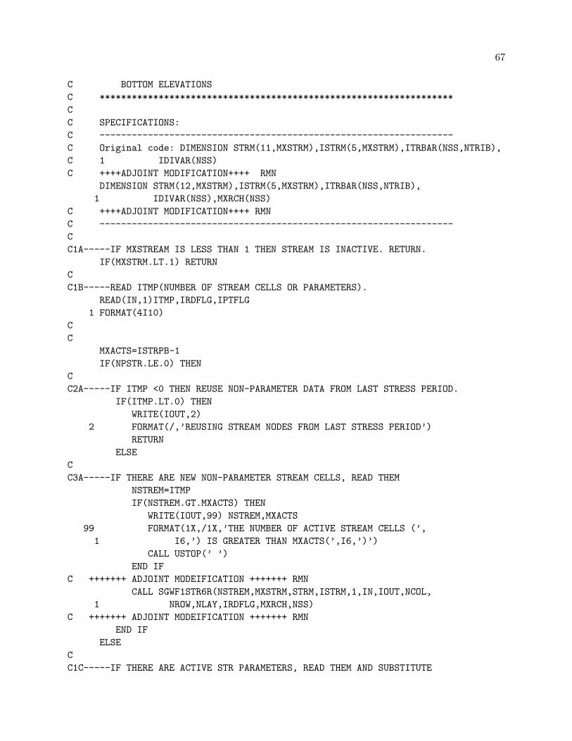
67

C BOTTOM ELEVATIONS

C ******************************************************************

C

C SPECIFICATIONS:

C ------------------------------------------------------------------

C Original code: DIMENSION STRM(11,MXSTRM),ISTRM(5,MXSTRM),ITRBAR(NSS,NTRIB),

C 1 IDIVAR(NSS)

C ++++ADJOINT MODIFICATION++++ RMN

DIMENSION STRM(12,MXSTRM),ISTRM(5,MXSTRM),ITRBAR(NSS,NTRIB),

1 IDIVAR(NSS),MXRCH(NSS)

C ++++ADJOINT MODIFICATION++++ RMN

C ------------------------------------------------------------------

C

C1A-----IF MXSTREAM IS LESS THAN 1 THEN STREAM IS INACTIVE. RETURN.

IF(MXSTRM.LT.1) RETURN

C

C1B-----READ ITMP(NUMBER OF STREAM CELLS OR PARAMETERS).

READ(IN,1)ITMP,IRDFLG,IPTFLG

1 FORMAT(4I10)

C

C

MXACTS=ISTRPB-1

IF(NPSTR.LE.0) THEN

C

C2A-----IF ITMP <0 THEN REUSE NON-PARAMETER DATA FROM LAST STRESS PERIOD.

IF(ITMP.LT.0) THEN

WRITE(IOUT,2)

2 FORMAT(/,’REUSING STREAM NODES FROM LAST STRESS PERIOD’)

RETURN

ELSE

C

C3A-----IF THERE ARE NEW NON-PARAMETER STREAM CELLS, READ THEM

NSTREM=ITMP

IF(NSTREM.GT.MXACTS) THEN

WRITE(IOUT,99) NSTREM,MXACTS

99 FORMAT(1X,/1X,’THE NUMBER OF ACTIVE STREAM CELLS (’,

1 I6,’) IS GREATER THAN MXACTS(’,I6,’)’)

CALL USTOP(’ ’)

END IF

C +++++++ ADJOINT MODEIFICATION +++++++ RMN

CALL SGWF1STR6R(NSTREM,MXSTRM,STRM,ISTRM,1,IN,IOUT,NCOL,

1 NROW,NLAY,IRDFLG,MXRCH,NSS)

C +++++++ ADJOINT MODEIFICATION +++++++ RMN

END IF

ELSE

C

C1C-----IF THERE ARE ACTIVE STR PARAMETERS, READ THEM AND SUBSTITUTE

68

NSTREM=0

CALL PRESET(’STR’)

IF(ITMP.GT.0) THEN

DO 100 N=1,ITMP

CALL UPARLSTLOC(IN,’STR’,IOUT,’STR’,IBEG,IEND,PV)

NLST=IEND-IBEG+1

NSTREM=NSTREM+NLST

IF(NLST.GT.MXACTS) THEN

WRITE(IOUT,99) NLST,MXACTS

CALL USTOP(’ ’)

END IF

DO 50 I=1,NLST

II=NSTREM-NLST+I

III=IBEG+I-1

DO 40 J=1,5

STRM(J,II)=STRM(J,III)

ISTRM(J,II)=ISTRM(J,III)

40 CONTINUE

STRM(3,II)=STRM(3,II)*PV

IF(IRDFLG.EQ.0) THEN

IF (N.EQ.1 .AND. I.EQ.1) WRITE(IOUT,4)

4 FORMAT(/,4X,’LAYER ROW COL SEGMENT REACH STREAMFLOW’,

16X,’STREAM STREAMBED STREAMBED BOT STREAMBED TOP’,/27X,

2’NUMBER NUMBER STAGE CONDUCTANCE’,6X,

3’ELEVATION ELEVATION’,/3X,110(’-’))

WRITE(IOUT,6)(ISTRM(J,II),J=1,5),(STRM(J,II),J=1,5)

ENDIF

6 FORMAT(1X,1X,I6,2I7,2I9,7X,G11.4,G12.4,G11.4,4X,2G13.4)

50 CONTINUE

C

100 CONTINUE

END IF

END IF

C

C3------PRINT NUMBER OF REACHES IN CURRENT STRESS PERIOD.

WRITE (IOUT,101) NSTREM

101 FORMAT(1X,/1X,I6,’ STREAM REACHES’)

C

C4------IF THERE ARE NO STREAM REACHES THEN RETURN.

IF(NSTREM.EQ.0) RETURN

C

C6----READ AND PRINT DATA IF STREAM STAGE IS CALCULATED.

IF(ICALC.LE.0) GO TO 300

IF(IRDFLG.EQ.0) WRITE(IOUT,7)

7 FORMAT(/,4X,’LAYER’,3X,’ROW’,4X,’COL ’,’ SEGMENT’,3X,

1’REACH’,8X,’STREAM’,13X,’STREAM’,10X,’ROUGH’,/27X,’NUMBER’,3X,

2 ’NUMBER’,8X,’WIDTH’,14X,’SLOPE’,10X,’COEF.’,/3X,110(’-’))

69

DO 280 II=1,NSTREM

READ(IN,8) STRM(6,II),STRM(7,II),STRM(8,II)

8 FORMAT(3F10.0)

IF(IRDFLG.EQ.0) WRITE(IOUT,9)ISTRM(1,II),

& ISTRM(2,II),ISTRM(3,II),ISTRM(4,II),ISTRM(5,II),

1 STRM(6,II),STRM(7,II),STRM(8,II)

9 FORMAT(2X,I6,2I7,2I9,7X,G12.4,4X,G13.4,4X,G12.4)

280 CONTINUE

C

C7------INITIALIZE ALL TRIBUTARY SEGMENTS TO ZERO.

300 DO 320 IK=1,NSS

DO 320 JK=1,NTRIB

ITRBAR(IK,JK)=0

320 CONTINUE

C

C8-----INITIALIZE DIVERSION SEGMENT ARRAY TO ZERO.

DO 325 IK=1,NSS

IDIVAR(IK)=0

325 CONTINUE

C

C9-----READ AND PRINT TRIBUTARY SEGMENTS.

IF(NTRIB.LE.0) GO TO 343

IF(IRDFLG.EQ.0) WRITE(IOUT,10)NTRIB

10 FORMAT(/,30X,’MAXIMUM NUMBER OF TRIBUTARY STREAMS IS ’,I6,//1X,

1 20X,’STREAM SEGMENT’,15X,’TRIBUTARY STREAM SEGMENT NUMBERS’)

DO 340 IK=1,NSS

READ(IN,11) (ITRBAR(IK,JK),JK=1,NTRIB)

11 FORMAT(10I5)

IF(IRDFLG.EQ.0) WRITE(IOUT,12) IK,(ITRBAR(IK,JK),JK=1,NTRIB)

12 FORMAT(19X,I6,20X,10I5)

340 CONTINUE

C

C10----READ AND PRINT DIVERSION SEGMENTS NUMBERS.

343 IF(NDIV.LE.0) GO TO 350

IF(IRDFLG.EQ.0) WRITE(IOUT,13)

13 FORMAT(/,10X,’DIVERSION SEGMENT NUMBER’,10X,

1 ’UPSTREAM SEGMENT NUMBER’)

DO 345 IK=1,NSS

READ(IN,14) IDIVAR(IK)

14 FORMAT(I10)

IF(IRDFLG.EQ.0) WRITE(IOUT,15) IK,IDIVAR(IK)

15 FORMAT(19X,I6,27X,I6)

345 CONTINUE

C

C11----SET FLOW OUT OF REACH, FLOW INTO REACH, AND FLOW THROUGH

C STREAM BED TO ZERO.

350 DO 360 II =1,NSTREM

70

STRM(9,II)=0.0

STRM(10,II)=0.0

STRM(11,II)=0.0

360 CONTINUE

C

C12------RETURN

RETURN

END

C ORIGINAL CODE

C SUBROUTINE GWF1STR6FM(NSTREM,STRM,ISTRM,HNEW,HCOF,RHS,IBOUND,

C 1 MXSTRM,NCOL,NROW,NLAY,NSS,ITRBAR,NTRIB,ARTRIB,

C 2 IDIVAR,NDFGAR,ICALC,CONST)

C ++++++++ ADJOINT MODIFICIATION +++++++ RMN

SUBROUTINE GWF1STR6FM(NSTREM,STRM,ISTRM,HNEW,HCOF,RHS,IBOUND,

1 MXSTRM,NCOL,NROW,NLAY,NSS,ITRBAR,NTRIB,ARTRIB,

2 IDIVAR,NDFGAR,ICALC,CONST,MXRCH)

C ++++++++ ADJOINT MODIFICIATION +++++++ RMN

C

C-----VERSION 15APRIL1998 GWF1STR6FM

C C

C *****************************************************************C

C ADD STREAM TERMS TO RHS AND HCOF IF FLOW OCCURS IN MODEL CELL C

C *****************************************************************C

C C

C SPECIFICATIONS: C

C -----------------------------------------------------------------C

C C

DOUBLE PRECISION HNEW

C Original code: DIMENSION STRM(11,MXSTRM),ISTRM(5,MXSTRM),HNEW(NCOL,NROW,NLAY),

C 1 HCOF(NCOL,NROW,NLAY),RHS(NCOL,NROW,NLAY),

C 2 IBOUND(NCOL,NROW,NLAY),ITRBAR(NSS,NTRIB),ARTRIB(NSS),

C 3 IDIVAR(NSS),NDFGAR(NSS)

C ++++ADJOINT MODIFICATION++++ RMN

DIMENSION STRM(12,MXSTRM),ISTRM(5,MXSTRM),HNEW(NCOL,NROW,NLAY),

1 HCOF(NCOL,NROW,NLAY),RHS(NCOL,NROW,NLAY),

2 IBOUND(NCOL,NROW,NLAY),ITRBAR(NSS,NTRIB),ARTRIB(NSS),

3 IDIVAR(NSS),NDFGAR(NSS),MXRCH(NSS)

C ++++ADJOINT MODIFICATION++++ RMN

C -----------------------------------------------------------------C

C C

C1------IF NSTREM<=0 THERE ARE NO STREAMS. RETURN. C

IF(NSTREM.LE.0)RETURN

C C

C2A-----PROCESS EACH CELL IN THE STREAM LIST. C

C2B-----INITIALIZE NDFGAR ARRAY TO ZERO. C

71

DO 5 I=1,NSS

NDFGAR(I)=0

5 CONTINUE

C C

C3------DETERMINE LAYER, ROW, COLUMN OF EACH REACH. C

C Original Code:

C DO 500 L=1,NSTREM

C LL=L-1

C ++++ADJOINT MODIFICATION++++

DO 500 LNEW=1,NSTREM

L=NSTREM-LNEW+1

LL=L+1

C ++++ADJOINT MODIFICATION++++

IL=ISTRM(1,L)

IR=ISTRM(2,L)

IC=ISTRM(3,L)

C C

C4----06FEB1990, CHECK FOR CELLS OUTSIDE MOVED TO C12, C16 AND C18. C

C C

C5------DETERMINE STREAM SEGMENT AND REACH NUMBER. C

ISTSG=ISTRM(4,L)

NREACH=ISTRM(5,L)

C C

C6------SET FLOWIN EQUAL TO STREAM SEGMENT INFLOW IF FIRST REACH. C

C ORIGINAL CODE:

C IF(NREACH.GT.1) GO TO 200

C FLOWIN=STRM(1,L)

C ++++ADJOINT MODIFICATION++++ RMN

IF (NREACH.LT.MXRCH(ISTSG)) GO TO 200

FLOWIN=STRM(1,L)

C ++++ADJOINT MODIFICATION++++ RMN

C C

C7------STORE OUTFLOW FROM PREVIOUS SEGMENT IN ARTRIB IF SEGMENT >1. C

C ORIGINAL CODE:

C IF(ISTSG.EQ.1)GO TO 50

C IFLG = ISTRM(4,LL)

C ARTRIB(IFLG)=STRM(9,LL)

C ++++ADJOINT MODIFICATION++++ RMN

IFLG = ISTRM(4,LL)

C ++++ADJOINT MODIFICATION++++ RMN

C C

C8A-----CHECK UPSTREAM SEGMENT FOR DIVERSIONS. C

DO 40 NSFLG = 1,NSS

IF(IFLG.NE.IDIVAR(NSFLG)) GO TO 40

C C

C8B-----DETERMINE AMOUNT OF FLOW TO BE DIVERTED. C

DO 20 IDL=1,NSTREM

72

IF(NSFLG.NE.ISTRM(4,IDL)) GO TO 20

IF(ISTRM(5,IDL).NE.1) GO TO 20

DUM=ARTRIB(IFLG)-STRM(1,IDL)

C C

C8C-----SUBTRACT FLOW FROM UPSTREAM SEGMENT IF THERE IS ENOUGH FLOW C

C-------IN UPSTREAM SEGMENT. C

IF(DUM.GE.0.0) ARTRIB(IFLG)=DUM

IF(DUM.LT.0.0) NDFGAR(IFLG)=1

20 CONTINUE

40 CONTINUE

50 IF(IDIVAR(ISTSG).LE.0) GO TO 60

NDFLG=IDIVAR(ISTSG)

IF(NDFGAR(NDFLG).EQ.1) FLOWIN=0.0

60 IF(FLOWIN.GE.0.0) GO TO 300

C C

C9-----SUM TRIBUTARY OUTFLOW AND USE AS INFLOW INTO DOWNSTREAM SEGMENT.C

C ORIGINAL CODE

C FLOWIN =0.

C DO 100 ITRIB=1,NTRIB

C INODE=ITRBAR(ISTSG,ITRIB)

C IF(INODE.LE.0) GO TO 100

C FLOWIN=FLOWIN+ARTRIB(INODE)

C 100 CONTINUE

C ++++ADJOINT MODIFICATION++++ RMN

FLOWIN=ARTRIB(ISTSG)

C ++++ADJOINT MODIFICATION++++ RMN

C C

C10-----IF REACH >1, SET INFLOW EQUAL TO OUTFLOW FROM UPSTREAM REACH. C

C ORIGINAL CODE:

C 200 IF(NREACH.GT.1) FLOWIN=STRM(9,LL)

C ++++ ADJOINT MODIFICATION +++++ RMN

200 IF (NREACH.LT.MXRCH(ISTSG)) FLOWIN=STRM(9,LL)

C ++++ ADJOINT MODIFICATION +++++ RMN

C C

C11----COMPUTE STREAM STAGE IN REACH IF ICALC IS GREATER THAN 1. C

300 IF(ICALC.LE.0) GO TO 310

C Original code:

C XNUM=((FLOWIN+STRM(9,L))/2.0)*STRM(8,L)

C DNOM=CONST*STRM(6,L)*(SQRT(STRM(7,L)))

C DEPTH=(XNUM/DNOM)**0.6

C

C ++++Adjoint Modification++++

XNUM=3.0*((FLOWIN+STRM(9,L))/2.0)*STRM(8,L)

DNOMA=5.0*CONST*STRM(6,L)*(SQRT(STRM(7,L)))

DNOMB=(STRM(12,L)-STRM(5,L))**(2.0/3.0)

DNOM=DNOMA*DNOMB

DEPTH=XNUM/DNOM

73

C ++++Adjoint Modification++++

IF(DEPTH.LE.0.) DEPTH=0.

STRM(2,L)=DEPTH+STRM(5,L)

310 HSTR=STRM(2,L)

C C

C12----DETERMINE LEAKAGE THROUGH STREAMBED. C

IF(IBOUND(IC,IR,IL).LE.0) GO TO 315

IF(FLOWIN.LE.0.) HSTR=STRM(5,L)

CSTR=STRM(3,L)

SBOT=STRM(4,L)

H=HNEW(IC,IR,IL)

T=HSTR-SBOT

C C

C13----COMPUTE LEAKAGE AS A FUNCTION OF STREAM STAGE AND HEAD IN CELL. C

C Original code: FLOBOT=CSTR*(HSTR-H)

C

C ++++Adjoint Modification++++

FLOBOT=(CSTR*(HSTR-H))

C ++++Adjoint Modification++++

C C

C14----RECOMPUTE LEAKAGE IF HEAD IN CELL IS BELOW STREAMBED BOTTOM. C

IQFLG=0

IF(H.GT.SBOT) GO TO 312

IQFLG=1

FLOBOT=CSTR*T

C C

C15----SET LEAKAGE EQUAL TO STREAM INFLOW IF LEAKAGE MORE THAN INFLOW. C

312 IF(FLOBOT.LE.FLOWIN) GO TO 320

IQFLG=1

FLOBOT=FLOWIN

C C

C16-----STREAMFLOW OUT EQUALS STREAMFLOW IN MINUS LEAKAGE. C

315 IF(IBOUND(IC,IR,IL).LE.0) FLOBOT=0.

320 FLOWOT=FLOWIN-FLOBOT

C ORIGINAL CODE (DELETED FROM ADJOINT MODIFICATIONS) RMN

C IF((ISTSG.GT.1).AND.(NREACH.EQ.1)) STRM(9,LL)=ARTRIB(IFLG)

C

C17----STORE STREAM INFLOW, OUTFLOW AND LEAKAGE FOR EACH REACH. C

STRM(9,L)=FLOWOT

STRM(10,L)=FLOWIN

STRM(11,L)=FLOBOT

C ++++ADJOINT MODIFICATION++++ RMN

IF (NREACH.GT.1) GO TO 201

DO 30 ITRIB=1,NTRIB

INODE=ITRBAR(ISTSG,ITRIB)

IF (INODE.NE.0) ARTRIB(INODE)=STRM(9,L)

30 CONTINUE

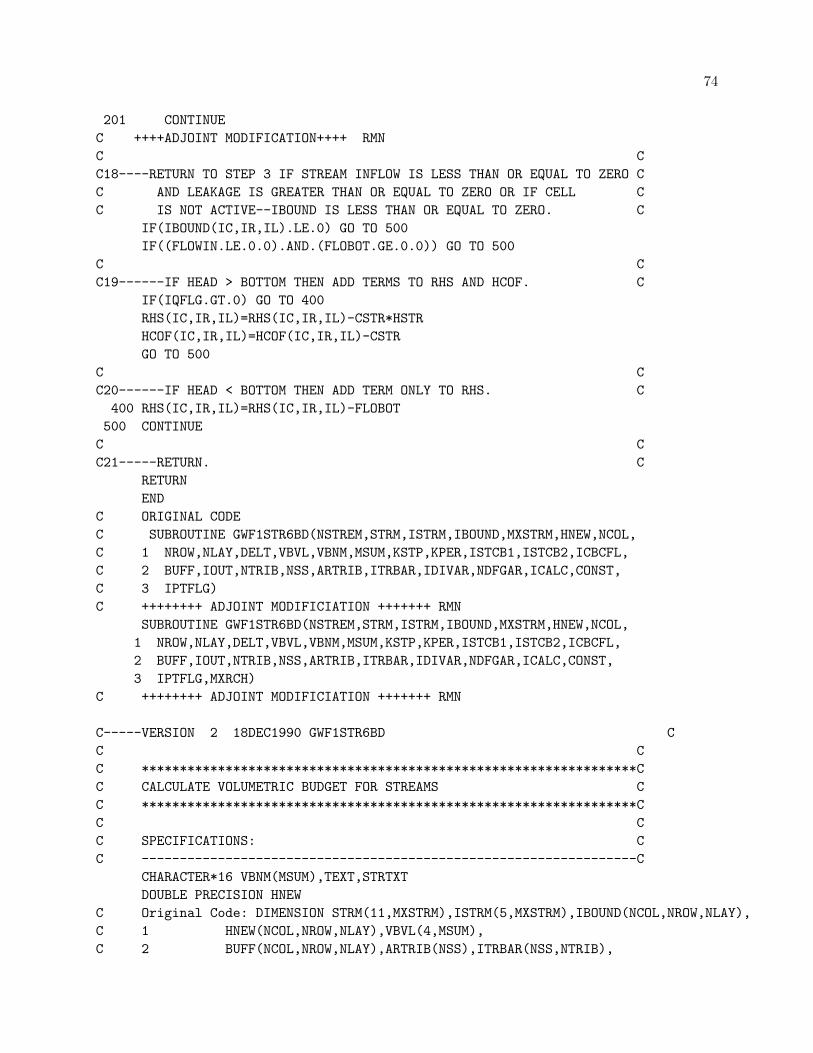
74

201 CONTINUE

C ++++ADJOINT MODIFICATION++++ RMN

C C

C18----RETURN TO STEP 3 IF STREAM INFLOW IS LESS THAN OR EQUAL TO ZERO C

C AND LEAKAGE IS GREATER THAN OR EQUAL TO ZERO OR IF CELL C

C IS NOT ACTIVE--IBOUND IS LESS THAN OR EQUAL TO ZERO. C

IF(IBOUND(IC,IR,IL).LE.0) GO TO 500

IF((FLOWIN.LE.0.0).AND.(FLOBOT.GE.0.0)) GO TO 500

C C

C19------IF HEAD > BOTTOM THEN ADD TERMS TO RHS AND HCOF. C

IF(IQFLG.GT.0) GO TO 400

RHS(IC,IR,IL)=RHS(IC,IR,IL)-CSTR*HSTR

HCOF(IC,IR,IL)=HCOF(IC,IR,IL)-CSTR

GO TO 500

C C

C20------IF HEAD < BOTTOM THEN ADD TERM ONLY TO RHS. C

400 RHS(IC,IR,IL)=RHS(IC,IR,IL)-FLOBOT

500 CONTINUE

C C

C21-----RETURN. C

RETURN

END

C ORIGINAL CODE

C SUBROUTINE GWF1STR6BD(NSTREM,STRM,ISTRM,IBOUND,MXSTRM,HNEW,NCOL,

C 1 NROW,NLAY,DELT,VBVL,VBNM,MSUM,KSTP,KPER,ISTCB1,ISTCB2,ICBCFL,

C 2 BUFF,IOUT,NTRIB,NSS,ARTRIB,ITRBAR,IDIVAR,NDFGAR,ICALC,CONST,

C 3 IPTFLG)

C ++++++++ ADJOINT MODIFICIATION +++++++ RMN

SUBROUTINE GWF1STR6BD(NSTREM,STRM,ISTRM,IBOUND,MXSTRM,HNEW,NCOL,

1 NROW,NLAY,DELT,VBVL,VBNM,MSUM,KSTP,KPER,ISTCB1,ISTCB2,ICBCFL,

2 BUFF,IOUT,NTRIB,NSS,ARTRIB,ITRBAR,IDIVAR,NDFGAR,ICALC,CONST,

3 IPTFLG,MXRCH)

C ++++++++ ADJOINT MODIFICIATION +++++++ RMN

C-----VERSION 2 18DEC1990 GWF1STR6BD C

C C

C *****************************************************************C

C CALCULATE VOLUMETRIC BUDGET FOR STREAMS C

C *****************************************************************C

C C

C SPECIFICATIONS: C

C -----------------------------------------------------------------C

CHARACTER*16 VBNM(MSUM),TEXT,STRTXT

DOUBLE PRECISION HNEW

C Original Code: DIMENSION STRM(11,MXSTRM),ISTRM(5,MXSTRM),IBOUND(NCOL,NROW,NLAY),

C 1 HNEW(NCOL,NROW,NLAY),VBVL(4,MSUM),

C 2 BUFF(NCOL,NROW,NLAY),ARTRIB(NSS),ITRBAR(NSS,NTRIB),

75

C 3 IDIVAR(NSS),NDFGAR(NSS)

C ++++ADJOINT MODIFICATION++++

DIMENSION STRM(12,MXSTRM),ISTRM(5,MXSTRM),IBOUND(NCOL,NROW,NLAY),

1 HNEW(NCOL,NROW,NLAY),VBVL(4,MSUM),

2 BUFF(NCOL,NROW,NLAY),ARTRIB(NSS),ITRBAR(NSS,NTRIB),

3 IDIVAR(NSS),NDFGAR(NSS),MXRCH(NSS)

C ++++ADJOINT MODIFICATION++++

DATA TEXT/’ STREAM LEAKAGE’/

DATA STRTXT/’STREAM FLOW OUT ’/

C -----------------------------------------------------------------C

C C

WRITE(IOUT,*) ISTRM(1,10),ISTRM(2,10),ISTRM(3,10), ISTRM(4,10)

C1------SET IBD=1 IF BUDGET TERMS SHOULD BE SAVED ON DISK. C

IBD=0

RATIN = 0.

RATOUT = 0.

C C

C2------IF NO REACHES, KEEP ZEROS IN ACCUMULATORS. C

IF(NSTREM.EQ.0) GO TO 600

C C

C3A-----TEST TO SEE IF CELL-BY-CELL TERMS ARE NEEDED. C

IF((ICBCFL.EQ.0).OR.(ISTCB1.LE.0)) GO TO 10

C C

C3B-----CELL-BY-CELL TERMS ARE NEEDED, SET IBD AND CLEAR BUFFER. C

IBD = 1

DO 5 IL=1,NLAY

DO 5 IR=1,NROW

DO 5 IC=1,NCOL

BUFF(IC,IR,IL)=0.

5 CONTINUE

C C

C3C-----INITIALIZE NDFGAR ARRAY TO ZERO. C

DO 7 I=1,NSS

NDFGAR(I)=0

7 CONTINUE

C C

WRITE(*,*) NSTREM

C4------IF THERE ARE STREAMS THEN ACCUMULATE LEAKAGE TO OR FROM THEM. C

C Original Code:

C 10 DO 500 L=1,NSTREM

C LL=L-1

C ++++ADJOINT MODIFICATION++++

10 DO 500 LNEW=1,NSTREM

L=NSTREM-LNEW+1

LL=L+1

C ++++ADJOINT MODIFICATION++++

C C

76

C5---DETERMINE REACH LOCATION. C

IL=ISTRM(1,L)

IR=ISTRM(2,L)

IC=ISTRM(3,L)

C C

C6----06FEB1990, CHECK FOR CELLS OUTSIDE MOVED TO C14, C18 AND C29. C

C C

C7------DETERMINE SEGMENT AND REACH NUMBER. C

ISTSG=ISTRM(4,L)

NREACH=ISTRM(5,L)

C ORIGINAL CODE:

C IF(NREACH.GT.1) GO TO 200

C C

C8------SET FLOWIN EQUAL TO SEGMENT INFLOW IF FIRST REACH. C

C FLOWIN=STRM(1,L)

C ++++ADJOINT MODIFICATION++++ RMN

IF (NREACH.LT.MXRCH(ISTSG)) GO TO 200

FLOWIN=STRM(1,L)

C ++++ADJOINT MODIFICATION++++ RMN

C C

C9------STORE OUTFLOW FROM PREVIOUS SEGMENT IN ARTRIB IF SEGMENT >1. C

C ORIGINAL CODE:

C IF(ISTSG.EQ.1) GO TO 50

C IFLG = ISTRM(4,LL)

C ARTRIB(IFLG)=STRM(9,LL)

C ++++ADJOINT MODIFICATION++++ RMN

IFLG = ISTRM(4,LL)

C ++++ADJOINT MODIFICATION++++ RMN

C C

C10A----CHECK UPSTREAM SEGMENT FOR DIVERSIONS. C

DO 40 NSFLG = 1,NSS

IF(IFLG.NE.IDIVAR(NSFLG)) GO TO 40

C C

C10B----DETERMINE AMOUNT OF FLOW TO BE DIVERTED. C

DO 20 IDL=1,NSTREM

IF(NSFLG.NE.ISTRM(4,IDL)) GO TO 20

IF(ISTRM(5,IDL).NE.1) GO TO 20

DUM=ARTRIB(IFLG)-STRM(1,IDL)

C C

C10C----SUBTRACT FLOW FROM UPSTREAM SEGMENT IF THERE IS ENOUGH FLOW C

C IN UPSTREAM SEGMENT. C

IF(DUM.GE.0.0) ARTRIB(IFLG)=DUM

IF(DUM.LT.0.0) NDFGAR(IFLG)=1

20 CONTINUE

40 CONTINUE

50 IF(IDIVAR(ISTSG).LE.0) GO TO 60

NDFLG=IDIVAR(ISTSG)

77

IF(NDFGAR(NDFLG).EQ.1) FLOWIN=0.0

60 IF(FLOWIN.GE.0.0) GO TO 300

C C

C11--SUM TRIBUTARY OUTFLOW AND USE AS INFLOW INTO DOWNSTREAM SEGMENT. C

C ORIGINAL CODE:

C FLOWIN =0.

C DO 100 ITRIB=1,NTRIB

C INODE=ITRBAR(ISTSG,ITRIB)

C IF(INODE.LE.0) GO TO 100

C FLOWIN=FLOWIN+ARTRIB(INODE)

C 100 CONTINUE

C ++++ADJOINT MODIFICATION++++ RMN

FLOWIN=ARTRIB(ISTSG)

C ++++ADJOINT MODIFICATION++++ RMN

C C

C12-----IF REACH >1, SET INFLOW EQUAL TO OUTFLOW FROM UPSTREAM REACH. C

C ORIGINAL CODE:

C 200 IF(NREACH.GT.1) FLOWIN=STRM(9,LL)

C ++++ ADJOINT MODIFICATION +++++ RMN

200 IF (NREACH.LT.MXRCH(ISTSG)) FLOWIN=STRM(9,LL)

C ++++ ADJOINT MODIFICATION +++++ RMN

C C

C13----COMPUTE STREAM STAGE IN REACH IF ICALC > 1. C

300 IF(ICALC.LE.0) GO TO 310

C Orignial Code:

C XNUM=((FLOWIN+STRM(9,L))/2.0)*STRM(8,L)

C DNOM=CONST*STRM(6,L)*(SQRT(STRM(7,L)))

C DEPTH=(XNUM/DNOM)**0.6

C

C ++++Adjoint Modification++++

XNUM=3.0*((FLOWIN+STRM(9,L))/2.0)*STRM(8,L)

DNOMA=5.0*CONST*STRM(6,L)*(SQRT(STRM(7,L)))

DNOMB=(STRM(12,L)-STRM(5,L))**(2.0/3.0)

DNOM=DNOMA*DNOMB

DEPTH=XNUM/DNOM

C ++++Adjoint Modification++++

IF((DEPTH).LE.0) DEPTH=0.

STRM(2,L)=DEPTH+STRM(5,L)

310 HSTR=STRM(2,L)

C C

C14----DETERMINE LEAKAGE THROUGH STREAMBED. C

IF(IBOUND(IC,IR,IL).LE.0) GO TO 315

IF(FLOWIN.LE.0.0) HSTR=STRM(5,L)

CSTR=STRM(3,L)

SBOT=STRM(4,L)

H=HNEW(IC,IR,IL)

T=HSTR-SBOT

78

C C

C15----COMPUTE LEAKAGE AS A FUNCTION OF STREAM STAGE AND HEAD IN CELL. C

C Original code: FLOBOT=CSTR*(HSTR-H)

C ++++Adjoint Modification++++

FLOBOT=(CSTR*(HSTR-H))

C ++++Adjoint Modification++++

C C

C16----RECOMPUTE LEAKAGE IF HEAD IN CELL IS BELOW STREAMBED BOTTOM. C

IF(H.GT.SBOT) GO TO 312

FLOBOT=CSTR*T

C C

C17----SET LEAKAGE EQUAL TO STREAM INFLOW IF LEAKAGE MORE THAN INFLOW. C

312 IF(FLOBOT.LE.FLOWIN) GO TO 320

FLOBOT=FLOWIN

C C

C18----STREAMFLOW OUT EQUALS STREAMFLOW IN MINUS LEAKAGE. C

315 IF(IBOUND(IC,IR,IL).LE.0) FLOBOT=0.

320 FLOWOT=FLOWIN-FLOBOT

C ORIGINAL CODE (DELETED FROM ADJOINT MODIFICATIONS) RMN

C IF((ISTSG.GT.1).AND.(NREACH.EQ.1)) STRM(9,LL)=ARTRIB(IFLG)

C C

C19----STORE STREAM INFLOW, OUTFLOW AND LEAKAGE FOR EACH REACH. C

STRM(9,L)=FLOWOT

STRM(10,L)=FLOWIN

STRM(11,L)=FLOBOT

C C

C ++++ADJOINT MODIFICATION++++ RMN

IF (NREACH.GT.1) GO TO 201

DO 30 ITRIB=1,NTRIB

INODE=ITRBAR(ISTSG,ITRIB)

IF (INODE.NE.0) ARTRIB(INODE)=STRM(9,L)

30 CONTINUE

201 CONTINUE

C ++++ADJOINT MODIFICATION++++ RMN

C20----IF LEAKAGE FROM STREAMS IS TO BE SAVED THEN ADD RATE TO BUFFER. C

IF(IBD.EQ.1) BUFF(IC,IR,IL)=BUFF(IC,IR,IL)+FLOBOT

C C

C21----DETERMINE IF FLOW IS INTO OR OUT OF MODEL CELL. C

C SKIP ESTIMATE OF LEAKAGE FROM STREAM IF LEAKAGE IS ZERO. C

IF(FLOBOT)494,500,496

C C

C22-----SUBTRACT FLOW RATE FROM RATOUT IF AQUIFER DISCHARGES TO STREAM.C

494 RATOUT=RATOUT-FLOBOT

GO TO 500

C C

C23-----ADD FLOW RATE TO RATIN IF STREAM DISCHARGES TO AQUIFER. C

496 RATIN=RATIN+FLOBOT

79

500 CONTINUE

C C

C24-----IF BUDGET TERMS WILL BE SAVED THEN WRITE TO DISK. C

IF(IBD.EQ.1) CALL UBUDSV(KSTP,KPER,TEXT,ISTCB1,BUFF,NCOL,NROW,

1 NLAY,IOUT)

C C

C25A-----MOVE RATES INTO VBVL FOR PRINTING BY MODULE BAS_OT. C

600 VBVL(3,MSUM)=RATIN

VBVL(4,MSUM)=RATOUT

C C

C25B-----MOVE PRODUCT OF RATE AND TIME STEP INTO VBVL ACCUMULATORS. C

VBVL(1,MSUM)=VBVL(1,MSUM)+RATIN*DELT

VBVL(2,MSUM)=VBVL(2,MSUM)+RATOUT*DELT

C C

C25C-----MOVE BUDGET TERM LABELS INTO VBNM FOR PRINTING BY BAS_OT. C

VBNM(MSUM)=TEXT

C C

C26-----INCREASE BUDGET TERM COUNTER BY ONE. C

MSUM=MSUM+1

C C

C27-----RESET IBD COUNTER TO ZERO. C

IBD=0

C28----IF STREAM OUTFLOW FROM EACH REACH IS TO BE STORED ON DISK C

C THEN STORE OUTFLOW RATES TO BUFFER. C

IF((ICBCFL.EQ.0).OR.(ISTCB2.LE.0)) GO TO 625

IBD = 1

DO 605 IL=1,NLAY

DO 605 IR=1,NROW

DO 605 IC=1,NCOL

605 BUFF(IC,IR,IL)=0.

C C

C29-----SAVE STREAMFLOWS OUT OF EACH REACH ON DISK. C

DO 615 L=1,NSTREM

IC=ISTRM(3,L)

IR=ISTRM(2,L)

IL=ISTRM(1,L)

IF(IBOUND(IC,IR,IL).LE.0) GO TO 615

BUFF(IC,IR,IL)=BUFF(IC,IR,IL)+STRM(9,L)

615 CONTINUE

CALL UBUDSV(KSTP,KPER,STRTXT,ISTCB2,BUFF,NCOL,NROW,NLAY,IOUT)

C C

C30-----PRINT STREAMFLOW RATES AND LEAKAGE FOR EACH REACH. C

625 IF((ISTCB1.GE.0).OR.(ICBCFL.LE.0)) GO TO 800

IF(IPTFLG.GT.0) GO TO 800

IF(ICALC.GT.0) GO TO 700

WRITE(IOUT,650)

650 FORMAT(/,12X,’LAYER’,6X,’ROW’,5X,’COLUMN’,5X,’STREAM’,4X,

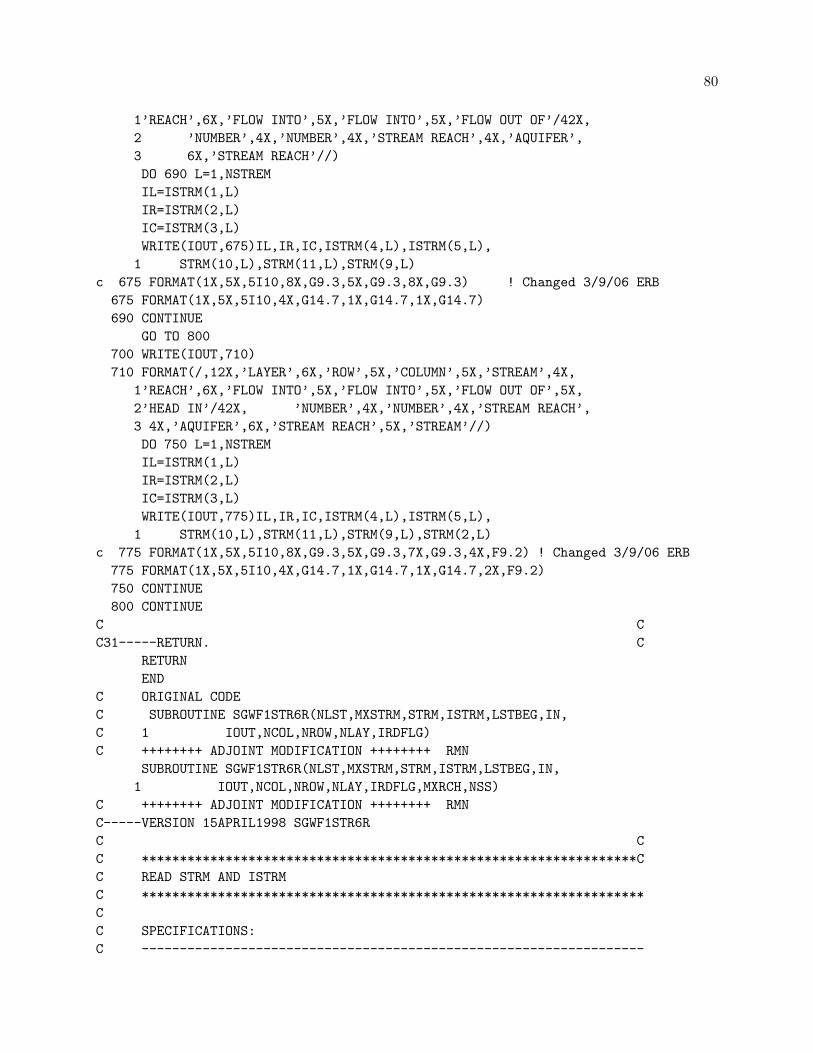
80

1’REACH’,6X,’FLOW INTO’,5X,’FLOW INTO’,5X,’FLOW OUT OF’/42X,

2 ’NUMBER’,4X,’NUMBER’,4X,’STREAM REACH’,4X,’AQUIFER’,

3 6X,’STREAM REACH’//)

DO 690 L=1,NSTREM

IL=ISTRM(1,L)

IR=ISTRM(2,L)

IC=ISTRM(3,L)

WRITE(IOUT,675)IL,IR,IC,ISTRM(4,L),ISTRM(5,L),

1 STRM(10,L),STRM(11,L),STRM(9,L)

c 675 FORMAT(1X,5X,5I10,8X,G9.3,5X,G9.3,8X,G9.3) ! Changed 3/9/06 ERB

675 FORMAT(1X,5X,5I10,4X,G14.7,1X,G14.7,1X,G14.7)

690 CONTINUE

GO TO 800

700 WRITE(IOUT,710)

710 FORMAT(/,12X,’LAYER’,6X,’ROW’,5X,’COLUMN’,5X,’STREAM’,4X,

1’REACH’,6X,’FLOW INTO’,5X,’FLOW INTO’,5X,’FLOW OUT OF’,5X,

2’HEAD IN’/42X, ’NUMBER’,4X,’NUMBER’,4X,’STREAM REACH’,

3 4X,’AQUIFER’,6X,’STREAM REACH’,5X,’STREAM’//)

DO 750 L=1,NSTREM

IL=ISTRM(1,L)

IR=ISTRM(2,L)

IC=ISTRM(3,L)

WRITE(IOUT,775)IL,IR,IC,ISTRM(4,L),ISTRM(5,L),

1 STRM(10,L),STRM(11,L),STRM(9,L),STRM(2,L)

c 775 FORMAT(1X,5X,5I10,8X,G9.3,5X,G9.3,7X,G9.3,4X,F9.2) ! Changed 3/9/06 ERB

775 FORMAT(1X,5X,5I10,4X,G14.7,1X,G14.7,1X,G14.7,2X,F9.2)

750 CONTINUE

800 CONTINUE

C C

C31-----RETURN. C

RETURN

END

C ORIGINAL CODE

C SUBROUTINE SGWF1STR6R(NLST,MXSTRM,STRM,ISTRM,LSTBEG,IN,

C 1 IOUT,NCOL,NROW,NLAY,IRDFLG)

C ++++++++ ADJOINT MODIFICATION ++++++++ RMN

SUBROUTINE SGWF1STR6R(NLST,MXSTRM,STRM,ISTRM,LSTBEG,IN,

1 IOUT,NCOL,NROW,NLAY,IRDFLG,MXRCH,NSS)

C ++++++++ ADJOINT MODIFICATION ++++++++ RMN

C-----VERSION 15APRIL1998 SGWF1STR6R

C C

C *****************************************************************C

C READ STRM AND ISTRM

C ******************************************************************

C

C SPECIFICATIONS:

C ------------------------------------------------------------------

81

C Original code: DIMENSION STRM(11,MXSTRM),ISTRM(5,MXSTRM)

C ADJOINT MODIFICATION***********************************************************************************************

DIMENSION STRM(12,MXSTRM),ISTRM(5,MXSTRM),MXRCH(NSS)

C ADJOINT MODIFICATION***********************************************************************************************

C ------------------------------------------------------------------

C

C5------READ AND PRINT DATA FOR EACH STREAM CELL.

IF(IRDFLG.EQ.0) WRITE(IOUT,4)

4 FORMAT(/,4X,’LAYER ROW COL SEGMENT REACH STREAMFLOW’,

16X,’STREAM STREAMBED STREAMBED BOT STREAMBED TOP’,/27X,

2’NUMBER NUMBER STAGE CONDUCTANCE’,6X,

3’ELEVATION ELEVATION’,/3X,110(’-’))

N=NLST+LSTBEG-1

DO 250 II=LSTBEG,N

C Original code: READ(IN,5)K,I,J,ISTRM(4,II),ISTRM(5,II),STRM(1,II),STRM(2,II),

C 1STRM(3,II),STRM(4,II),STRM(5,II)

C 5 FORMAT(5I5,F15.0,4F10.0)

C IF(IRDFLG.EQ.0) WRITE(IOUT,6)K,I,J,ISTRM(4,II),

C 1ISTRM(5,II),STRM(1,II),STRM(2,II),STRM(3,II),STRM(4,II),STRM(5,II)

C 6 FORMAT(1X,1X,I6,2I7,2I9,7X,G11.4,G12.4,G11.4,4X,2G13.4)

C ++++ADJOINT MODIFICATION++++

READ(IN,5)K,I,J,ISTRM(4,II),ISTRM(5,II),STRM(1,II),STRM(2,II),

1STRM(3,II),STRM(4,II),STRM(5,II),STRM(12,II)

C ++++ FOLLOWING LINE ADDED FOR TRIBUTARY ADJOINT MODIFICATION ++++ RMN

MXRCH(ISTRM(4,II))=ISTRM(5,II)

5 FORMAT(5I5,F15.0,5F10.0)

IF(IRDFLG.EQ.0) WRITE(IOUT,6)K,I,J,ISTRM(4,II),ISTRM(5,II),

1STRM(1,II),STRM(2,II),STRM(3,II),STRM(4,II),STRM(5,II),STRM(6,II)

6 FORMAT(1X,1X,I6,2I7,2I9,7X,G11.4,G12.4,G11.4,4X,3G13.4)

C ++++ADJOINT MODIFICATION++++

ISTRM(1,II)=K

ISTRM(2,II)=I

ISTRM(3,II)=J

C

C Check for illegal grid location

IF(K.LT.1 .OR. K.GT.NLAY) THEN

WRITE(IOUT,*) ’ Layer number in list is outside of the grid’

CALL USTOP(’ ’)

END IF

IF(I.LT.1 .OR. I.GT.NROW) THEN

WRITE(IOUT,*) ’ Row number in list is outside of the grid’

CALL USTOP(’ ’)

END IF

IF(J.LT.1 .OR. J.GT.NCOL) THEN

WRITE(IOUT,*) ’ Column number in list is outside of the grid’

CALL USTOP(’ ’)

END IF

82

250 CONTINUE

C

RETURN

END