Pushover CE&CR

8/20/2019 Pushover CE&CR

http://slidepdf.com/reader/full/pushover-cecr 1/9

ThePushoverAnalysisn ItsSimplicity

Rahul Leslie, Assistant Director Buildings Design DRIQ Board Kerala PWD Trivandrum

eismic esign

One of the emerging fields in seismic design of structures is the

Performance ased Design The subject is still in the realm of

research and academics and is only slowly emerging out into the

practitioner s arena. Seismic design is transforming from a stage

where a linear elastic analysisfor a structure was sufficient for both

its elastic and ductile design to a stage where a specially dedicated

non-linear procedure is to be done

which finally influences

the

seismic design as a whole.

The basis for the linear approach lies in the concept of the

Response Reduction factor R. When a structure is designed for a

ResponseReduction factor of say R = 5 it means that 115thof the

seismic force istaken by the Limit State capacity. Further deflection

Theneedfora simplemethodto predictthenon-linear

behaviourofa structureunderseismicloadssawlightin

whatisnowpopularlyknownasthe PushoverAnalysis PA .

It canhelpdemonstratehowprogressiveailurein buildings

reallyoccurs,andidentifythe modeof finalfailure.

is in its ductile behaviour and istaken by the ductile capacity of the

structure. In Reinforced Concrete RC) structures, the members

beams and columns) are detailed such as to make sure that the

structure can take the full impact without collapse beyond its Limit

State capacity up to its ducti le capacity. Infact we never analyse for

the ductile part, but only follow the reinforcement detailing guidelines

for the same. The drawback is that the response beyond the limit

state is neither a simple extrapolation, nor a perfectly ductile

behaviour with pre-determinable deformation capacity. This is due

to various reasons: the change in stiffness of members due to

cracking and yielding, P-delta effects, change in the final seismic

force estimated, to list a few - putting vaguely. Although elastic

ana~sis gives a good indication of elastic capacity of structures and

shows where yielding will first occur, it cannot account for

redistribution of forces during the progressive yielding that follows

and predict its failure mechanisms, or detect possibility and location

of any premature failure. A non-linear static analysiscanpredict these

more accurately since it considers the inelast ic behaviour of the

structure. It can help identify critical members likely to reach critica

states during an earthquake for which attention should be give

during design and detailing.

The need for asimple method to predict the non-linear behaviou

of astructure under seismic loads saw light in wh,at is now popularl

known as the Pushover Analysis PA). It can help demonstrate how

progressive failure in buildings really occurs, and identify the mod

of final failure. Putting simply, PAis a non-linear analysis procedur

to estimate the strength capacity of a structure beyond its elasti

limit meaning Limit State) up to its ultimate strength in the post

elastic range. Inthe process, the method also predicts potential wea

areas in the structure, by keeping track of the sequence of damage

of eachand every member in the structure by useof what arecalle

hinges they hold).

Pushover Versus onventional nalysis

In order to understand PA, the best approach would be to first se

the similarities between PA and the conventional seismic analys

SA), both Seismic Coefficient and Response Spectrum method

described in IS:1893, which most of the readers are familiar with

and then see how they are different.

Both SAand PAapply lateral load of a predefined pattern on th

structure. InSA, the lateral load isdistributed either parabolicall

in Seismic Coefficient method) or proportional to the mod

combination in Response Spectrum method). In PA, the

distribution is proportional to height raised to the power of k

where k can be equal to 0 uniform distribution), 1 the inverted

triangle distribution), 2 parabolic distribution as in the seism

coeff icient method) or any value between 1 and 2, the value o

k being based on certain criteria listed inthe FEMA 356 Federa

Emergency Management Agency, USA) code. The distribution

can also be proportional to either the first mode shape, or

combination of modes.

In both SA and PA, the maximum lateral load estimated for th

structure iscalculated based on the fundamental time period o

the structure.

And the last point above is precisely where the difference starts

While inSAthe initial time period istaken to be a constant, in PAthi

is continuously re-calculated as the analysis progresses. Th

differences between the procedures are as follows:

118

CE CR JUNE 2 1



SA uses an elastic model, while PAuses a non-linear model. In

the latter this is incorporated in the form of non-linear hinges

inserted into an otherwise linear elastic model which one

generates using a common analysis-design software package,

but of course, using one that has facilities for PA.

The Hinges

inges are points on a structure where one expects cracking and

eldingto occur inrelatively higher intensity so that they show high

exural (or shear) displacement, as it approaches its ultimate

rength. These are locations where one expects to see cross diagonal

acks in an actual building structure after a seismic mayhem and

y would be at either end of beams and columns, the cross being

a smalldistance from the joint - that is where one is expected to

ert the hinges inthe corresponding computer model. Hinges are

various types - namely, flexural hinges, shear hinges and axial

nges. The first two are inserted into the ends of beams and columns.

cethe presenceof masonry

infill hassignificantinfluence

onthe

ismic behaviour of the structure, modelling them using equivalent

agonal struts is common inPA,unlike inthe conventional analysis,

re its inclusionisa rarity.Theaxialhingesare insertedat either

d of the diagonal struts thus modelled, to simulate cracking of

llduring analysis.

Basicallya hinge represents localised force-displacement relation

a member through its elastic and inelastic phases under seismic

ads. For example, a flexural hinge represents the moment-rotation

lation of a beam of which a typical one is as represented in Fig.1.

represents the linearrange from unloaded state (A)to its effective

eld (B), followed by an inelastic but linear response of reduced

stiffness

fromBtoC.CDshowsa suddenreductioninload

sistance, followed by a reduced resistance from Dto E,and finally

total lossof resistance from Eto F.Hingesare inserted ina framed

ucture typicallyas showninFig.2.Thesehingeshavenon-linear

sdefinedas ImmediateOccupancy 10), Life Safety LS) and

Prevention CP)within its ductile

range.

Thisisusuallydone

by dividing BC into

four parts and denoting

. ,

.

D

~9

M

E

F

9~

Fig. 1: A

Typical Flexural Hinge Property,

howing

ImmediateOccupancy ,LS

e Safety and CP Collapse Prevention

10, LS and CP,which are

states of each individual

hinges in spite of the

fact that the structure as

a whole too have these

states defined by drift

limits).

Flexural hinge

Shear hinge

xial hinge

Fig.2: Typical Locations of Hinges in a Structural Model

The Two Stage esign pproach

Although hinge properties can be obtained from charts of average

values included in FEMA356, ATC-40 Applied Technoiogy Council

USA) and FEMA 440 - which are only rough estimates - for accurate

results, one requires the details of reinforcement provided in orde

to calculate exact hinge properties using concrete models such a

Mander model available in SAP2000 software package). And one

has to design the structure in order to obtain the reinforcement

details. This means that PA i s meant to be a second stage analysis

Thusthe new methodology to a seismic design is:first a linear seismi

analysis based on which a primary structural design isdone; insertion

of hinges determined based on the design and then a pushover

analysis, followed by modification of the design and detailing,

wherever necessary, based on the latter analysis.

On SA, the analysis results are always the elastic limit state

forces moment, shear and axial forces) to be designed for. In PA, i

the global sense,it isthe baseshear Vb) versus rooftop displacemen

ClrOOftopaken as displacement of a point on the roof, located in pla

at the centre of mass), plotted up to the termination of the analysis

At a local level, it is t he hinge states to be examined and decided o

the need for its redesign or a retrofit.

PAcanbe useful under two situations: When an existing structure

has deficiencies in seismic resisting capacity due to either omissio

of seismic design when built, or the structure becoming seismicall

inadequate due to a later upgrading of the seismic codes) is to b

retrofitted to meet the present seismic demands, PAcan show where

the retrofitting is required and how much. In fact this was what P

was originally developed for, and for which it is st ill widely used. Fo

a building in its design phase, PAresults help scrutinise and fine tune

the seismic design based on SA, which in future will turn out to b

more of a standard procedure.

CR JUNE 2012

11



SA, being a linear analysis, is done independently for dead and

live loads, and the results combined to give the design forces. But

since PAisnon-linear, gravity and lateral loadsare applied sequentially

for the analysis. In SA, the loads are factored, since the results are

for the design, but since PAisdone to simulate the behaviour under

actual loads, the loads applied are not factored. The gravity loads

are applied inaccordance with CI.7.3.3 and Table8 of IS:1893-2002,

giving a combination of [DL + 0.25 LL 3kN/SQ.m0.5 LL>3kN/Sqml

InSA, the lateral load of acalculated intensity isapplied inwhole

- in one shot. In PA, structure model (ie., the- computer model) is

gently pushed over by a monotonically increasing lateral load applied

in steps up to a predetermined value or state.

This predetermined value or state depends on the method used.

One is the F M 356 method, where a Target Displacement is

calculated to which the structure is pushed . The other is the

ATC-40 method, where the load isincremented until what is called

the Performance Point condition is reached. In this article, only the

ATC-40 method is dealt with, since it is found to be more suitable

for RCCstructures.

The Single egree Of Freedom Idealization

One of the fundamental simplifications underlying the concept of

PA is that it considers the structure as a single degree of freedom

(SDOF) system, which in reality it hardly is. And that means the

structure model, with numerous joints with lumped masses, is

assumed to be a single vertical strut fixed at bottom with a single

(but considerable) mass lumped at the top. This makes one aspect

of the procedure ignore that the structure has numerous joints with

different values of damping (depending on the level of damage each

suffers), leaving it with just a single global value to deal with.

Equations have been developed (ATC-40, 1996) to arrive at this

equivalent damping ratio ~,and also time period T(both continuously

changing due to the weakening of hinges in course of the analysis)

at any particular point incourse of the progress of the analysis, having

knownonly the instantaneous

~rooftop

andVb of the structure.

The cceleration isplacement

Response Spectra

Another innovative concept incorporated inthe PAisthe Acceleration

Displacement Response Spectra (ADRS) representation, which

mergesthe Vbversus~rooftoP plot with the ResponseSpectrum(RS)

curve. This is possible due to a relation connecting Vb, ~roofopand

T.First the Vb versus ~roOftopartesian hasto betransformed to what

iscalled spectral acceleration (Sa) versus spectral displacement (Sd)

using the relations

TC-40, 1996)

v:

IW

Sa =

b

xg

Mk 1M

1 )

~ rooftop

Sd=

Pk fjJk,rooftop

(2)

where Mk Pkand

<f>k.rooftop

(using the notation of IS:1893) are modal

mass, mode participation factor and modal amplitude at rooftop

respectively for the first mode (k=1). M and Ware the total mass

and weight of the building. Next the RSgraph, having axes Saand T

has to be converted using the relation TC-40, 1996)

T2

Sd =~Sa

41Z

(3)

Thus T, which was along the x-axis in the RScurve, is marked as

radial lines in the transformed plot (Fig.3). Using the above relation,

the time period T represented by a radial line drawn from the origin

through any point (Sd, Sa) can befound. The two transformed plots,

one that of Vb versus ~rooftop and the other the RScurve - now known

as the capacity and demand curves respectively - can be

superimposed to get the ADRSplot.

The PAhas not been introduced in the Indian Standard code yet.

However the procedure described inATC-40 can be adapted for the

seismic parameters of IS:1893-2002. The RScurve in ATC-40 is

described by parameters Ca and Cv, where the curve just as in

IS:1893, ishaving a flat portion of intensity 2.5 Caand a downward

sloping portion described by Cv/T (Fig.4a). The seismic force in

21

sa

)

S:1893 is represented by 2R

g

, where Sa/g is obtained from

the RScurve which on the other hand is represented by 2.5 in the

T-0.5,

t

~

Sd -.

Fig :ADRSRepresentationf TheResponsepectrumCurve

120 CE CR JUNE 2012





0

0.25

2,5'(ZI2)

0.2

0.15

Sa

9

0.1

0.05

0

0 N ~ ~ ~ N ~ ~ N N ~ ~ ~ N ~ ~ ~

000 ~ ~ ~ N N N M M M

~ ~ ~ N ~ ~ ~ v ~ ~ ~ ~ ~

6 6 6 ~ ~ ~ N N N M M M

T(s)

T(s)

a

ResponsepectrumCurvea describednATC-40and b definednIS:1893,hownhereforDBE,Zone-IIInotconsideringandRfactors ,Mediumoi

b

Vbqlu - n - - --- - - - - - - ~Q

I

t

a

.<>

>

Vbp - - -- ---

I1p

I1q ~rooftop ~

b

t

.

.

So f \O

Sop -

Tp

T-

t

c

c::

5 ------------

Fig.5: a Vb vs .1roOftOPlot, b Response spectrum and

c ADRSplotforconventionaleismicanalysis

flat portion and the downward sloping portion by 1/T, 1.36/T and 1.67/T for

hard, medium and soft soils respectively (Fig.4b). Oncomparison it can be inferred

that Ca = Z/2 and Cv= Z/2, 1.36.Z/2 and 1.67.Z/2 respectively for DBE(Design

Base Earthquake - which is the one meant for design). Here 'I' (the importance

factor as per Table6 of IS:1893-2002) is not considered, since inPA,the criteria

of importance of the structure is taken care of by the performance levels (of 10,

LSand CP) instead. R is also not considered since PAisalways done for the full

lateral load.

tep y tep Through ach ethod

Now let's first see what's actually happening in the SAprocedure and then trace

the progress of a PAfrom beginning to end, both using plots of Vbversus ~rooft

and RScurve inits separate and uncombined form and alsotheir transformed and

super-positioned ADRSplot.

Z

sa

n SA, the maximum DBEforce acting on the structure is 'I' times 2 g

,

(assuming Ito be unity) with Sa/g corresponding to the estimated time period. Its

envelop isthe RScurve marked q inFig.5b. The RScurve for the LimitState design

Z

sa

s plotted in terms

of2R g

,and is marked as curve p. Fig.5a shows the Vb vs

~rooftopisplacement. Nowassume a structure (Fig.7a) subjected to a SA.ln Fig.5a,

the point P represents the Vb and ~rooftopor the design lateral load (ie., of 1/R

times fullload) while Q represents the same for the fullload, had the buildingbeen

fully elastic (and Q' for a perfectly-elastic perfectly-ductile structure). The slope

of the lineOP represents the stiffness of the structure in a globalsense. Since the

analysis is linear,the stiffness remains same throughout the analysis, with Q being

an extension of or. The same is represented in Fig.5b where, for the time period

Tpof the structure, the full load is represented by Q, and the design force by P

The

ADRS

representationof SAisas inFig.5c.

CE CR JUNE 2012



Vbcf- - u -- - - .

Vbb u - -8 - uu

P

t

.Q

>

a

.6.c Arooftop ~

6.a

.6.b

t

b

'~~

. .~

0

~

Vbc

Vbb

Vb.

T. TbTc

T~

t

c

..

'

-Vb,.. .

Sd~

Fig.6:

a Vb vs L1rooffoP

lot, b) Responsespectrumand

c)ADRSplotforpushoveranalysis

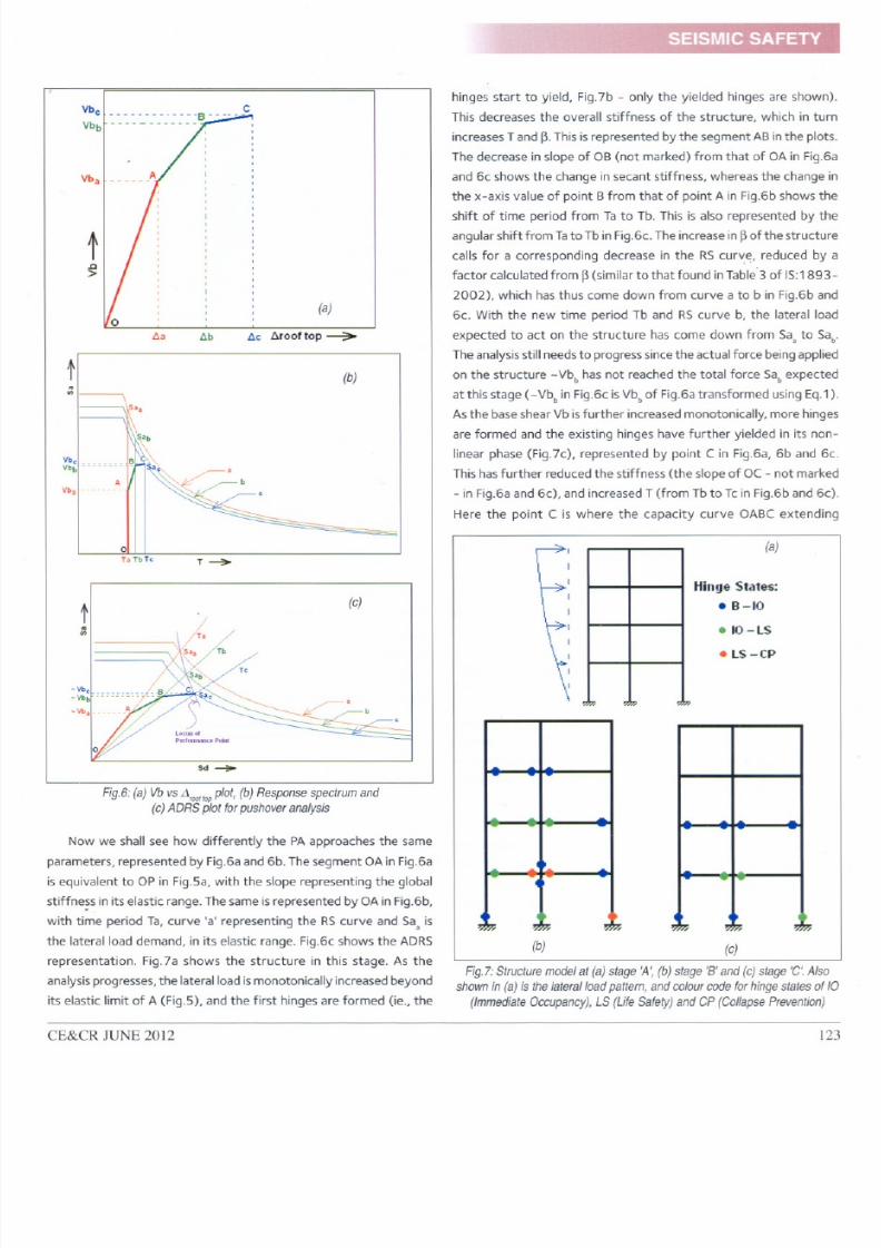
Now we shall see how differently the PA approaches the same

rameters, represented by Fig.6a and 6b. The segment OA in Fig.6a

equivalent to OP in Fig.Sa, with the slope representing the global

iffne~~ in its elastic range. The same isrepresented by OA in Fig.6b,

ith time period Ta, curve 'a' representing the RScurve and Sa, is

e lateral load demand, in its elastic range. Fig.6c shows the ADRS

epresentation. Fig.7a shows the structure in this stage. As the

lysis progresses, the lateral load is monotonically increased beyond

ts elastic limit of A (Fig.5), and the first hinges are formed (ie., the

SEISMIC SAFETY

hinges start to yield, Fig.7b - only the yielded hinges are shown).

This decreases the overall stiffness of the structure, which in turn

increases T and ~.This isrepresented by the segment AB inthe plots.

The decrease in slope of OB (not marked) from that of OA in Fig.6a

and 6c shows the change in secant stiffness, whereas the change in

the x-axis value of point B from that of point A in Fig.6b shows the

shift of time period from Ta to Tb. This is also represented by the

angular shift from Tato Tb in Fig.6c. The increase in~of the structure

calls for a corresponding decrease in the RScur~e, reduced by a

factor calculated from

~

(similar to that found inTable'3 of IS:1893-

2002 ,

which has thus come down from curve a to b in Fig.6b and

6c. With the new time period Tb and RS curve b, the lateral load

expected to act on the structure has come down from Sa, to Sab.

The analysisstill needs to progress since the actual force being applied

on the structure -Vbb has not reached the total force Sabexpected

at this stage (- Vbbin Fig.6c isVbbof Fig.6a transformed using Eq.1).

As the baseshear Vb isfurther increased monotonically, more hinges

are formed and the existing hinges have further yielded in its non-

linear phase (Fig.7c), represented by point C in Fig.6a, 6b and 6c.

This has further reduced the stiffness (the slope of OC - not marked

- in Fig.6a and 6c), and increased T (from Tb to Tcin Fig.6b and 6c).

Here the point C is where the capacity curve OABC extending

a

Hinge States:

.8-10

.IO-LS

. LS-CP

b)

c)

Fig.?:Structuremodelat a)stage A , b)stageB and c)stageC .Also

shownn a)isthelateraloadpattern,andcolourcodeforhingestatesof 10

ImmediateOccupancy),S LifeSafety)and CollapsePrevention)

E CR JUNE 2012 123

, ,

. ,

-

.,\ ; 'i ,

- - -

'i '/ 'i ,



.

upwards with the increase in lateral push meets the demand curve in

Fig.6c, which was simultaneously descending down to curve c due

to increase in ~.Thus C is the point where the total lateral force

expected Sacis same as the lateral force applied -Vbc - this point is

known asthe performance point. It isalsodefined asthe point where

the 'locus of the performance point', the line connecting Sa Sab

and Sac(the load demands for points A, B, C in Fig.6c), intersects

the capacity curve (which is,in general, the method used by software

packages to determine the performance point). Of course, it can

happen that if the structure is seismically weak, it can reach its

collapse mechanism before the capacity curve can meet the

descending demand curve, denying the structure of a performance

point.

The procedure elaborated above is done automatical ly by any

structural package providing PAfacility. Once the performance point

is found, the overall performance of the structure can be checked

to see whether it matches the required performance level of 10, LS

or CP, based on drift limits specified in ATC-40 which are 0.01 h,

0.02h and 0.33(Vb/W).h respectively (h being the height of the

building). The performance level is based on the importance and

function of the building. For example, hospitals and emergency

services buildings are expected to meet a performance level of 10.

Infact these limits are more stringent than those specified inIS:1893.

The 'Limit State' drifts of 0.004 specified in the latter, when

accounted for R (= 5 for ductile desi gn) and I (taken as 1.5 for

important structures which demand an 10performance level) gives

0.004.R/1 = 0.0133, which is more than the 0.01 allowed in

ATC-

40. This 0.004.R/1 can be taken as the IS:1893 limits for pushover

drift, where I takes the value corresponding to Important and

Ordinary structures for limits of 10 and LSrespectively.

The next step isto review the hinge formations at performance

point. One can see the individual stage of each hinge, at its location.

Tables are obtained showing the number of hinges in each state, at

each stage, based on which one decides which all beams and columns

to be redesigned. The decision depends whether the most severely

yielded hinges are formed in beams or in columns, whether they are

concentrated in a particular storey denoting soft story, and so on.

xample Of uilding nalysis

Presentedn this section are the results of a pushover analysis done

on a 10 storey RCCbuilding of a shopping complex (Jisha, 2008)

(Fig.8) using the structural package of SAP2000. In the model,

beams and columns were modelled using frame elements into which

the hinges were inserted. Diaphragm action was assignedto the floor

slabsto ensure integral lateral action of beams ineach floor. Although

analysis was done in both transverse and longitudinal directions, only

the results of the former are discussed here. The lateral load was

applied

in

pattern of that first mode shape inthe transverse direction

of the building, with an

intensity for DBE as per

IS:1893, corresponding to

zone-III in hard soil. Fig.9

shows the ADRS plot in

which the Sa and Sd at

performance point are

0.085g and 0.242m. The

correspondingVband ~roof

top are 1857.046 kN and

0.287m. The value of

effective T is 3.368s. The

effective ~at that level of

the demand curve which

Fig.8:A viewof the computermodelof

met the performance buildingbeinganalysed

point is 26%. Table 1

shows the hinge state detai ls at each step of the analysis. It can be

seen that for the performance point, taken as step 5 (although it

actually lies between steps 4 and 5), 95% of hinges are within LS

and 88% within 10 performance level. Fig.10a to 10e shows the

hingestatesduringvariousstagesincourseof the analysis.A~roofto

of 0.287 m, with the height of the building up to rooftop h (which

excludesthe staircasetower room) being36.8m, givesa ~rooftop

to h

ratio of 0.0078 in an average sense) which lies within the

performance level of 10.

L mitations

Assuch the method appears complete and sound, yet there are many

aspects which are unresolved, which include incorporation of

torsional effects, accounting for changes

in mode shapes as the

analysis

progresses,

etc. The most

addressed but yet unresolved)

issue is

that the procedure basically

takes

into account only the

SpectralDisplacement1m)

1.00~1

0,90:

0,80:

0.70:

.,

c:

i

]

i

~

0,60~

0,50-

0.40]

0,30

0,20:

0.10-

50, 250,

450, 500:~10.3

00.

350: 400,

00. 150: 200,

Fig.9:ADRSplotfortheanalysisCapacityurvengreen,demandcurvesn

red,andlocusofperformanceointindarkyellow

124

CE CR JUNE 2012

\

\

\

\

:1--

\\ \

\\ \

\\ ,,

'

>.

0

---..

-

r-----

-----

r----

---- ----.

-

:

-,-

'oo

'

--' I



HEY SAYTHE NEXT WORLD WAR WOULD BE FOUGHT IN WATER

....

-......--

11111

'f

'

1

,

-

II

,

..

I,'.'

$,/,

DURA@

PRODU TSFORW TERPROOFING

r:::jj='

DURACRIL: Acrylic liquid

waterproofing compound.

DURA 1:Waterproofer cum corrosion

inhibitor.

r:::jj='

WJMCRIST: Integral waterproofing by

fttfQ ling insoluble crystals.

IIIAJEL: Polymeric water reactive

chemical grout.

IIIJf4AMENJEL: Water based

rubberized bitumen jel.

;IIMKRIT: Waterproof breathable

cementitious acrylic polymer.

'IUIiaPAIR:

SBR polymer

for

repair and rehabilitation.

r:::jj='

r:::jj='

r:::jj='

DURAGARD: Polymeric cementitious

breathable waterproof coating.

DURAFEX: Polymer modified

flexible/Elastomeric Coating.

DURATITE: Integral waterproofing

cum plasticiser.

fr

r:::jj='

r:::jj='

r:::jj='

. t1J=

Note: All the construction chemical products mentioned above are being manufactured by us, as per National and International Quality Standard

DURfi UILD flREPVT LT

\\.1

@

DORA

AN ISO9001 : 2008 COMPANY

2«4tter

<?~

ri~,

..

104-106,

Dimension Deepti Plaza, Plot No.-3,

LSC,

Pocket - 6, Nasirpur, Dwarka, New Delhi -

110045

:011

-

25050236n, 65373673 Fax. : 011 - 25050238

E-mail: [email protected], [email protected]

Factory and R D Center Bahadurgarh, Haryana

Xlisit

us at{www.durabuildcare.com)fpf

fI}

. c



a

various solutions to this, a method is

yet to be set standard, and included in

the software packages. Moreover, the

PA method as such is yet to be

incorporated in the IndianStandards.

onclusions

The author has intended here to

explain the meth.()d with as much

simplicity as one could so as to

introduce the basic concepts to those

who are already familiar with the

conventional seismic analyses. It is

hoped that this aim has been fulfilled

to some extent. Of course, there are

many aspects which this article has

not touched upon - likeincorporating

soil structure interaction, deciding

different pushover analysis parameters,

modelling shear walls and flat slabs with

hinges, etc. - since this is not meant to

deal with the procedure to that extent.

Acknowledgement: The example of

pushover analysispresented inthis article

istaken from the academic work byJisha

S. V., a former PGstudent in Structural

Engineering, which is gratefully

acknowledged.

eference

1. IS 1893 (Part 1 )-2002, Indian Standard

Criteria for Earthquake Resistant Design of

Structures, Part 1: General Provision and

Buildings , Bureau of Indian Standards, New

Delhi

2.

FEMA 356 (2000) Prestandard and

Commentary for the Seismic Rehabilitation of

Buildings , Federal Emergency Management

Agency, Washington, DC, USA;

3.

ATC-40 (1996) Seismic Analysis and

Retrofit of Concrete Buildings , vol. I,Applied

Technology Council , Redwood City, CA,USA;

4. FEMA-440 2005 Improvement of

Nonlinear static seismic analysis procedures , Federal Emergency

Management Agency, Washington, DC, U.S.A.

5. SAP2000. Integrated software for structural analysis and design ,

Computers and Structures Inc., Berkeley, CA, USA.

6. Jisha S. V. (2008), Mini Project Report Pushover Analysis , Department

of Civil Engineering, T. K. M. College of Engineering, Kollam, Kerala.

e

II l

LS -CP

C-D

D-E

>E

Fig.10:Hinge states in the structure model at a step

0,

b step

3,

c step

5,

d step

8

and

e step 10during the pushover analysis, withcolourcodes of hinge st t s

ndamental mode as can beseen inthe procedure for transforming

and ~rooftop

to Saand Sd, explained earlier), assuming it to be the

redominant response and does not consider effects of higher

odes. The discrepancies due to this start to be felt for buildings

ith T over 1 second. Although many research papers proposed

Hinge

States

Step I tlrOOftOP (m)

I

Vb (kN) I

A to

Bto 10to LSto CPto C to

Dto Total

B 10 LS CP C

D E >E

Hinges

0

I

0

0 1752 0

0 0 0 0

0 0 1752

0.058318 1084.354 1748 4 0 0 0 0 0 0 1752

2

0.074442 1348.412 1670 82

0 0 0 0

0 0 1752

3

0.089645 1451.4

1594 158 0

0 0 0 0 0

1752

4 0.26199

1827.137

1448 168 136 0

0 0 0 0 1752

5 0.41105

2008.48 1384

144 136 88 0

0 0 0 1752

6 0.411066 1972.693

1384 146

136 86 0 0 0

0 1752

7

0.411082 1576.04

1376 148 136 39

0 0 53 0

1752

8

0.411098 1568.132

1376 148 136

37 0 0 55 0

1752

9 0.411114

1544.037 1375

149 136 31

0 0 61 0 1752

10 0.40107 1470.133 1375 149 136 31 0 0 61 0 1752

Documents

Pushover CE&CR