PULSED EDDY CURRENT INSPECTION OF …. Stott MASc Thesis... · Signed by the final examining committee: / Signé par les membres du comité examinateur de la soutenance de thèse

PULSED EDDY CURRENT INSPECTION OF

SECOND LAYER WING STRUCTURE

UTILISATION DES COURANTS DE FOUCAULT PULSÉS POUR

L’INSPECTION DE LA DEUXIÈME COUCHE STRUCTURALE

D’UNE AILE D’AVION

A Thesis Submitted

To the Division of Graduate Studies of the Royal Military College of Canada

by

Colette Amelia Stott

Captain

In Partial Fulfillment of the Requirements for the Degree of

Masters of Applied Science in Chemical and Materials Engineering

9 June 2014

©This thesis may be used within the Department of National Defence

but copyright for open publication remains the property of the author.

ii

ROYAL MILITARY COLLEGE OF CANADA COLLÈGE MILITAIRE ROYAL DU CANADA

DIVISION OF GRADUATE STUDIES AND RESEARCH DIVISION DES ÉTUDES SUPÉRIEURES ET DE LA RECHERCHE

This is to certify that the thesis prepared by / Ceci certifie que la thèse rédigée par

Colette Amelia Stott

entitled / intitulée

Pulsed Eddy Current Inspection of Second Layer Wing Structure /

Utilisation des courants de Foucault pulsés pour l’inspection de la deuxième couche structurale d’une aile d’avion

complies with the Royal Military College of Canada regulations and that it meets the accepted standards of the Graduate School with respect to quality,and, in the case of a doctoral thesis, originality, / satisfait aux

règlements du Collège militaire royal du Canada et qu'elle respecte les normes acceptées par la Faculté des études supérieures quant à la qualité et, dans le cas d'une thèse de doctorat, l'originalité,

for the degree of / pour le diplôme de

Master of Applied Science / Maîtrise en Science Appliquée

Signed by the final examining committee: / Signé par les membres du comité examinateur de la soutenance de thèse

__________________________,Chair / Président

__________________________, External Examiner / Examinateur externe

__________________________, Main Supervisor / Directeur de thèse principal

____________________________________________________

Approved by the Head of Department : / Approuvé par le Directeur du Département :______________ Date: ________

To the Librarian: This thesis is not to be regarded as classified. / Au Bibliothécaire : Cette thèse n'est pas considérée comme à publication restreinte.

____________________________________________

Main Supervisor / Directeur de thèse principal

iii

Acknowledgements

I would like to thank Dr. Krause, my thesis supervisor, for his guidance and patience throughout the

last two years. Your dedication to the Non-Destructive Testing field, as well as encouragement and

constructive feedback has greatly contributed to the success of this thesis.

I would also like to thank Dr. Underhill (Royal Military College of Canada Mechanical Engineering

Department) for his unwavering support, assistance in building probes, Labview programs and

whatever else I asked of him. Additionally I would like to thank Dr. Babbar (RMCC Physics

Department) for his research, COMSOL modelling and assistance in understanding electromagnetic

theories.

Additionally, I would like to thank Captain Alayne Edwards, Captain Ashley Oliver and Sgt James

Scalf from the Aerospace Technical Engineering Support Squadron (ATESS) for their help in

ordering parts for test pieces, and providing NDT expertise. Also, a special thank you is extended to

Dr. Sangalli (RMCC Physics Department) for the French translation of the title and abstract.

Finally, I would like to thank Chris for his patience and understanding throughout the last two years.

Your support has helped guide me through a great challenge and I could not have done it without

you.

iv

Abstract

A thesis completed by Stott, Colette Amelia, in partial fulfilment of the requirements for a MASc in

Chemistry and Materials Engineering from the Royal Military College of Canada on this 9th June,

2014 on Pulsed Eddy Current Inspection of Second Layer Wing Structure, under the direction of Dr. Thomas

Krause.

Non-destructive testing has become a valuable inspection tool for the aerospace industry. In

particular, eddy current testing is used extensively to detect surface and near surface defects in

aluminum aircraft component structures. However, there exists a requirement to inspect for the

presence of cyclic fatigue cracks around ferrous fasteners in the second layer of double layer

structures, such as the lap-joint of the CP-140 Aurora, and CC-130 Hercules. These defects are not

easily detectable by conventional eddy current techniques, unless the fasteners are removed. A

capability to inspect through the top layer would avoid fastener removal, in turn reducing down time

and risk of collateral damage to the structure. Pulsed eddy current (PEC) is an emerging technique

with the potential to detect cyclic fatigue cracking in the second layer of aluminum wing structures.

PEC offers potential advantages over conventional eddy current in that the inspection occurs from

the top layer, does not require fastener removal and the diffused magnetic field can be sensed at

greater depths within the material. However, the time-domain PEC signals show only subtle

differences between the presence or absence of cracks. Principal components analysis (PCA) is a

statistical tool that can be used to reduce the time domain signal to a small number of scores, which

enhance the distinction between PEC signals. These scores are clustered depending on whether a

crack is present. The relative distance (Mahalanobis Distance), between the scores for a crack and

the centroid of the scores for fasteners with no crack can be used to distinguish between cracks and

non-cracks.

A PEC coil-based probe was tested on three lap-joint samples containing ferrous fasteners, two of

which were actual CP-140 Aurora airframes, and one that was fabricated in the lab. Simulated flaws,

ranging in size from 0.8 - 5.5 mm, were present in both the top and bottom aluminum layers. One

hundred percent of the simulated flaws were detected in two of the samples with top sheet thickness

of 2 mm, and 82% in a thicker (2.6 mm thick first layer) airframe section with a different fastener

type, all at 5% false call rate. An observed correlation between Mahalanobis Distance and crack size

also suggested that sizing of second layer cracks is possible.

v

Résumé

Thèse complétée par Stott, Colette Amelia, pour l’obtention d’une MASc en Chimie et Génie des

Matériaux du Collège militaire royal du Canada ce 9 juin 2014 sur utilisation des courants de Foucault

pulsés pour l’inspection de la deuxième couche structurale d’une aile d’avion, sous la supervision directe de Dr

Thomas Krause.

Le contrôle non destructif est une technique de grande valeur pour l’industrie aérospatiale. En

particulier, les courants de Foucault sont largement utilisés pour détecter les défauts de surface ou

proche de la surface des composantes en aluminium dans les avions. Des critères d’inspection

existent pour estimer la présence de fissures dues à la fatigue cyclique autour des attaches en fer au

niveau de la deuxième couche d’une structure à deux couches, comme les joints de recouvrement des

ailes des avions Aurora CP-140 et Hercule CC-130. Ces défauts ne sont pas détectables facilement

avec les méthodes de courants de Foucault conventionnelles, à moins que les attaches en fer soient

retirées. La capacité d’accomplir l’inspection à travers la couche supérieure des ailes permettrait

d’éviter le retrait des attaches et donc de réduire la durée d’inspection et les risques collatéraux

d’endommagement de la structure. L’usage des courants de Foucault pulsés (CFP) est une méthode

relativement récente qui pourrait détecter les fissures dues à la fatigue cyclique dans la deuxième

couche structurale des ailes d’avions en aluminium. L’avantage des CFP par rapport aux méthodes

conventionnelles est que l’inspection est effectuée sans le retrait des attaches directement à travers la

couche externe de l’aile et le champ magnétique diffusé peut être détecté plus profondément dans le

matériau. Cependant, le signal des CFP dans le domaine temporel ne manifeste que de petites

différences en présence de fissure par rapport à celui mesuré quand aucune fissure n’est présente.

L’analyse en composantes principales (ACP) est un outil statistique qui peut être utilisé pour réduire

le signal temporel en un petit nombre de poids ce qui permet d’augmenter les différences entre les

signaux des CFP. Ces poids sont groupés en fonction de la présence de fissure. La distance relative

(distance de Mahalanobis) entre les poids en présence de fissures et le centroïde des poids quand il

n’y a pas de fissures, peut être utilisés pour distinguer les signaux dus sans fissures et avec fissures.

Une sonde CFP à base de bobines fut testée sur trois joints de recouvrement comprenant des

attaches ferreuses, deux joints proviennent d’avions Aurora CP-140 et le troisième fut fabriqué au

laboratoire. Des défauts allant de 0.8 à 5.5 mm furent crées à la fois dans première et la deuxième

couche d’aluminium. Cent pourcent des défauts furent détectés dans les deux échantillons possédant

une couche supérieure de 2 mm d’épaisseur et 82% des défauts furent détecté dans l’échantillon dont

vi

la couche supérieure mesure 2.6 mm d’épaisseur et avec différents types d’attaches, dans tous les cas

le taux de fausse détection est de 5%. La corrélation observée entre la distance de Mahalanobis et la

taille des fissures suggère qu’il est possible d’estimer la taille des défauts de la seconde couche.

vii

Table of Contents

Acknowledgements ........................................................................................................................................... iii

Abstract .............................................................................................................................................................. iv

Résumé ................................................................................................................................................................ v

List of Tables .................................................................................................................................................... xii

List of Figures .................................................................................................................................................. xiii

List of Abbreviations ...................................................................................................................................... xvi

1. Introduction ............................................................................................................................................... 1

1.1 General ................................................................................................................................................ 1

1.2 Eddy Current Testing ....................................................................................................................... 3

1.3 Research Survey ................................................................................................................................. 5

1.3.1 Analytical Work ......................................................................................................................... 5

1.3.2 Crack Detection in the Presence of Fasteners ...................................................................... 6

1.3.3 PEC Signal Analysis .................................................................................................................. 8

1.3.4 PEC signals and Principal Components Analysis .............................................................. 11

1.3.5 PCA and Mahalanobis Distance ........................................................................................... 13

1.4 Objective .......................................................................................................................................... 14

1.5 Thesis Scope and Methodology .................................................................................................... 14

2 Theory ....................................................................................................................................................... 16

2.1 General .............................................................................................................................................. 16

2.2 Maxwell’s Equations ....................................................................................................................... 16

2.3 Electromagnetic Waves in Conductors ........................................................................................ 17

2.4 Diffusion Equations ....................................................................................................................... 18

2.5 Charge dissipation in a conductor ................................................................................................ 20

2.6 Skin Depth Theory.......................................................................................................................... 20

viii

2.7 Eddy Current Generation .............................................................................................................. 21

2.8 Equivalent Circuit Diagram ........................................................................................................... 22

2.9 Principal Components Analysis (PCA) ........................................................................................ 26

2.9.1 General ..................................................................................................................................... 26

2.9.2 PCA Method ............................................................................................................................ 26

2.9.3 PCA Scores .............................................................................................................................. 29

2.10 Cluster Analysis Method ................................................................................................................ 30

2.10.1 Mahalanobis Distance Definition ......................................................................................... 30

2.10.2 Decision Threshold ................................................................................................................ 31

2.11 Probability of False Positive (False Calls) .................................................................................... 31

3 Experimental Technique ........................................................................................................................ 33

3.1 General .............................................................................................................................................. 33

3.2 Coil Probe Design ........................................................................................................................... 33

3.3 Sensing Equipment ......................................................................................................................... 34

3.4 Single Fastener Test Piece .............................................................................................................. 35

3.5 Multiple Fastener Test Pieces ........................................................................................................ 36

3.5.1 NAVAIR Sample Description .............................................................................................. 36

3.5.2 Test Piece #1 Description ..................................................................................................... 38

3.5.3 Test Piece #2 Description ..................................................................................................... 40

3.5.4 CP-140-TT-1B Test Piece ..................................................................................................... 40

3.6 Experimental Procedure ................................................................................................................. 42

3.6.1 Probe Alignment ..................................................................................................................... 42

3.6.2 Single Fastener Experimental Procedure ............................................................................ 44

3.6.3 Multiple Fastener Test Piece Experimental Procedure ..................................................... 45

3.7 Summary of Experiments .............................................................................................................. 45

3.8 Signal Processing ............................................................................................................................. 46

ix

3.8.1 Signal Gating ............................................................................................................................ 46

3.8.2 Signal Analysis ......................................................................................................................... 47

4 Results and Analysis of Single Fastener Case ...................................................................................... 49

4.1 General .............................................................................................................................................. 49

4.2 Off-Centering Effects ..................................................................................................................... 49

4.3 Notch Effects .................................................................................................................................. 51

5 Results and Analysis of Multiple Fastener Case .................................................................................. 54

5.1 General .............................................................................................................................................. 54

5.2 Off-Centering Effects ..................................................................................................................... 54

5.3 Notch Effects .................................................................................................................................. 57

5.4 Effect Due to Height of Fastener Head and Lift-Off ............................................................... 57

5.4.1 Fastener Head Height Effects ............................................................................................... 58

5.4.2 Lift-off Effects ........................................................................................................................ 61

5.5 Effect Due to Edge ......................................................................................................................... 62

5.6 Effect Due to Fastener Distance from Edge .............................................................................. 63

5.7 Effect of Temperature on Probe Performance .......................................................................... 65

5.8 Results on NAVAIR Sample ......................................................................................................... 65

5.8.1 Test Piece Summary ............................................................................................................... 65

5.8.2 Eigenvector Selection ............................................................................................................. 65

5.8.3 Absolute Mode Crack Detection Test Results ................................................................... 67

5.8.4 Differential Mode Crack Detection Test Results ............................................................... 69

5.8.5 Mahalanobis Distance versus Crack Size ............................................................................ 71

5.9 Results on Test Piece #1 ................................................................................................................ 72


5.9.2 Eigenvector Selection ............................................................................................................. 72

5.9.3 Absolute Mode Crack Detection Results ............................................................................ 73

x

5.9.4 Differential Mode Crack Detection Results ........................................................................ 75

5.9.5 Mahalanobis Distance versus Crack Size ............................................................................ 76

5.10 Results on Test Piece CP-140-TT-1B .......................................................................................... 77


5.10.2 Differential Mode Crack Detection Results ........................................................................ 77

5.10.3 Mahalanobis Distance versus Crack Size Results ............................................................... 79

5.11 Comparison of Test Piece Results (Differential Analysis) ........................................................ 80

6 Discussion ................................................................................................................................................. 82

6.1 PCA and Crack Orientation .......................................................................................................... 82

6.2 Absolute versus Differential Analysis .......................................................................................... 83

6.3 Comparison to FEM ....................................................................................................................... 84

6.4 PCA Score Correlations with Variables ....................................................................................... 84

6.5 Minimum Detectable Flaw Size .................................................................................................... 85

6.5.1 General ..................................................................................................................................... 85

6.5.2 First Layer Notches ................................................................................................................ 86

6.5.3 Second Layer Notch Detection ............................................................................................ 86

6.6 False Call Rates ................................................................................................................................ 87

6.7 Sources of Uncertainty ................................................................................................................... 87

6.7.1 Coil Balancing .......................................................................................................................... 87

7 Conclusions and Recommendations ..................................................................................................... 88

7.1 Conclusions ...................................................................................................................................... 88

7.2 Recommendations ........................................................................................................................... 89

References ......................................................................................................................................................... 92

Annex A ............................................................................................................................................................ 97

Annex B ............................................................................................................................................................. 98

Annex C............................................................................................................................................................. 99

xi

Curriculum Vitae ............................................................................................................................................ 102

xii

List of Tables

Table 1: Description of parameters for Figure 11. ..................................................................................... 23

Table 2: Driving coil and pick-up coil parameters. ..................................................................................... 34

Table 3: Single fastener case experimental parameters. .............................................................................. 36

Table 4: NAVAIR sample notch locations and lengths. ............................................................................ 38

Table 5: Test piece #1 notch parameters. .................................................................................................... 40

Table 6: CP-140-TT-1B notch parameters. .................................................................................................. 42

Table 7: Shimming experimental parameters. .............................................................................................. 44

Table 8: Number of measurements taken per test piece. ........................................................................... 45

Table 9: Summary table of experiments conducted on each test piece, in sequence. ............................ 45

Table 10: NAVAIR sample experimental cases for off-centering and notch effects on PCA scores. 54

Table 11: Test Piece #2 HL-19-5-5 fastener head height relative to aluminum surface, for no notch

sites. .................................................................................................................................................................... 58

Table 12: Distance from edge of fastener to edge of aluminum. ............................................................. 63

Table 13: NAVAIR Sample crack detection results in absolute mode. ................................................... 69

Table 14: NAVAIR Sample crack detection results in differential mode. ............................................... 70

Table 15: Test piece #1 crack detection results in absolute mode. .......................................................... 74

Table 16: Test Piece #1 crack detection results in differential mode. ..................................................... 75

Table 17: Test piece CP-140-TT-1B crack detection results in differential mode. ................................ 77

Table 18: Crack detection results for no false calls, 5% and 10% false call rate. ................................... 81

Table 19: Summary of PCA correlations with different variables. ........................................................... 85

xiii

List of Figures

Figure 1: Cross-section of lap joint (a), where the two sections are attached using a row of fasteners,

and (b) close up of crack location showing aspect ratio of 1:1. .................................................................. 2

Figure 2: Typical damage that can occur to wing skin during fastener removal. ..................................... 3

Figure 3: Front view of a solved 3D finite element half-model showing flux penetration through the

ferrous fastener (CDDP Probe design) [25]. ................................................................................................. 8

Figure 4: Typical PEC signal with common signal response analysis. ....................................................... 9

Figure 5: Time domain response from four fasteners, with and without notches. ................................ 10

Figure 6: Zoomed view of peaks from Figure 5.......................................................................................... 10

Figure 7: Zoomed view of zero-crossing from Figure 5. ........................................................................... 11

Figure 8: Sample and probe geometry used in FE models [32]. ............................................................... 13

Figure 9: RL circuit representing excitation coil.......................................................................................... 22

Figure 10: Current in driving coil representing equation 2.33. .................................................................. 23

Figure 11: Equivalent circuit diagram for driving coil and pick-up coil. ................................................. 24

Figure 12: Current response in pick-up coil representing equation 2.36 (i2). .......................................... 25

Figure 13: Three-way mutual inductance relationships between driving coil, pick-up coil and sample.

............................................................................................................................................................................ 26

Figure 14: PEC original signal with first eigenvector reproduction, and eigenvectors 1-4

reproduction. The insert shows the four eigenvectors for each coil of the pair, used for the

reproduction ..................................................................................................................................................... 29

Figure 15: PCA scores viewed in 3D, in the (a) un-rotated view and (b) rotated view for fasteners

with (●) and without (○) notches at their bore. ........................................................................................... 30

Figure 16: Probe face with central driving coil, ferrite core and eight pick-up coils. ............................ 33

Figure 17: Flow chart depiction of sensing equipment operation cycle. ................................................. 35

Figure 18: Side view of Single Fastener Test Piece with three plates and centrally located ferrous

fastener. ............................................................................................................................................................. 35

Figure 19: NAVAIR sample with notches, view from top. ....................................................................... 37

Figure 20: NAVAIR sample with view of fastener. .................................................................................... 37

Figure 21: View from top. Notch orientation diagram. ............................................................................ 37

Figure 22: Microscopic photo of notch cut into fastener hole (11x magnification). ............................. 39

Figure 23: Picture of test piece #1. ............................................................................................................... 39

Figure 24: Picture of section of CP-140-TT-1B test piece. ....................................................................... 41

xiv

Figure 25: Schematics of notches located at fasteners 9 and 19 of CP-140-TT-1B Aurora Sample. .. 41

Figure 26: Alignment tool, showing the direction of shimming (0° and 90°). ....................................... 43

Figure 27: Probe with alignment guide and sample. ................................................................................... 44

Figure 28: Raw PEC data signal from a fastener without a notch, indicating the gate. ........................ 46

Figure 29: Eddy current density curve from finite element modeling. .................................................... 47

Figure 30: Data processing sequence for PEC signals. .............................................................................. 48

Figure 31: Plot of PCA scores S2 versus S1 for single fastener with no notch, showing off-centered

results. ................................................................................................................................................................ 49


results. ................................................................................................................................................................ 50


results. ................................................................................................................................................................ 51

Figure 34: Plot of PCA scores S2 versus S1 for single fastener case of no notch (⟡), 2 mm (⧠) and 8

mm (∆) notch. Arrows indicate direction of increasing notch length. ..................................................... 52





Figure 37: Plot of S2 versus S1. Numbers correspond to Table 10 cases. For probe displacement

(disp), arrows indicate direction of increasing displacement. .................................................................... 55







Figure 41: Effect of fastener head height distance and lift-off distance on first PCA score (S1). ....... 59

Figure 42: Effect of fastener head height distance and lift-off distance on second PCA score (S2). . 59

Figure 43: Effect of fastener head height distance and lift-off distance on the third PCA score (S3).

............................................................................................................................................................................ 60

Figure 44: Effect of fastener head height distance and lift-off distance on the fourth PCA score (S4).

............................................................................................................................................................................ 60

xv

Figure 45: Effect of fastener head height distance and lift-off distance on the fifth PCA score (S5). 61

Figure 46: Experimental no-crack differential signals from all four coil pairs. ....................................... 63

Figure 47: PCA score S4 plotted with fastener distance to edge in millimeters. .................................... 64

Figure 48: PCA score S5 plotted with fastener distance to edge in millimeters. .................................... 64

Figure 49: First five eigenvectors of PCA on data from NAVAIR third coil pair (differential mode).

............................................................................................................................................................................ 66

Figure 50: Results from logistic regression performed on hit miss data from NAVAIR sample using

1-3, 1-4 and 1-5 eigenvectors. Horizontal axis is on a log scale. ............................................................... 67

Figure 51: 3-D view of NAVAIR data PCA scores S2, 3 & 4. ................................................................. 68

Figure 52: NAVAIR Sample Mahalanobis Distance versus fastener # in absolute mode. .................. 69

Figure 53: NAVAIR Sample Mahalanobis Distance versus fastener # in differential mode. .............. 70

Figure 54: Mahalanobis Distance versus crack size for NAVAIR Sample second layer cracks in

differential mode. ............................................................................................................................................. 71

Figure 55: First five eigenvectors of PCA on data from Test Piece #1 third coil pair (concatenated

signals) in absolute mode. ............................................................................................................................... 72

Figure 56: Results from logistic regression performed on hit miss data from Test Piece #1 using

eigenvectors 3-5 and 1-5. Horizontal axis is on a log scale........................................................................ 73

Figure 57: Test Piece#1 Mahalanobis Distance versus fastener # in absolute mode. .......................... 74

Figure 58: Test Piece#1 Mahalanobis Distance versus fastener # in differential mode. ...................... 75

Figure 59: Mahalanobis Distance versus crack size for Test Piece #1 in differential mode. ............... 76

Figure 60: CP-140-TT-1B Mahalanobis Distance versus fastener # in differential mode. .................. 78

Figure 61: Mahalanobis Distance versus crack size for test piece CP-140-TT-1B in differential mode.

............................................................................................................................................................................ 80

Figure 62: Three dimensional depiction of PCA scores S2, S3 and S4 from NAVAIR differential

data. Labels refer to notch orientation as defined in the inserted figure. ................................................ 83

xvi

List of Abbreviations

AC Alternating Current

ATESS Aerospace and Telecommunications Engineering Support Squadron

AWG American Wire Gauge

BHEC Bolt Hole Eddy Current

CDDP Central Driver Differential Pickup

CFRP Carbon Fiber Reinforced Polymer

CGSB Canadian General Standards Board

EDM Electrically Discharge Machining

EMF Electromotive Force

ET Eddy-Current Testing

FEM Finite Element Modelling

GMR Giant Magneto-resistive

IACS International Annealed Copper Standard

LPI Liquid Penetrant Inspection

MD Mahalanobis Distance

MPI Magnetic Particle Inspection

NDE Non-destructive Evaluation

NDT Non-destructive Testing

NI National Instruments

NN No Notch

PCA Principal Components Analysis

PEC Pulsed Eddy Current

POD Probability of Detection

SCC Stress Corrosion Cracking

UT Ultrasonic Testing

1

1. Introduction

1.1 General

The probability of failure of aircraft components in flight has been reduced by the implementation

of inspection programs. The application of non-destructive evaluation techniques (NDE) provides a

means of inspecting aircraft and their components for flaws or damage without ideally

compromising the component’s future use. The aerospace industry has introduced the application of

NDE techniques into inspection schedules with increasing age of military and civilian aircraft.

Additionally, scheduled maintenance periods may be lengthened with proper use of these techniques

in the maintenance cycle [1]. Non-destructive testing (NDT) techniques are similar to those of

NDE. However, NDE incorporates additional analysis of measurements that are more quantitative

in nature [2].

There are many different types of NDE methods but the only five certified NDT techniques of the

Canadian General Standards Board (CGSB) are: ultrasonic testing (UT), radiography, liquid

penetrant inspection (LPI), magnetic particle inspection (MPI) and eddy current [3]. Understanding

the physical basis of these techniques, along with their respective strengths and limitations, helps

determine reliable inspection criteria for the aerospace industry. Despite advances in technology,

there are still many inspection requirements that are beyond the capability of the five techniques

mentioned above, which drives research in the field of NDE.

The CP-140 Aurora and CC-130 Hercules aircraft most often employ the eddy current NDT

method because their aircraft structures are mainly composed of highly conducting aluminum

(30.0% - 31.4% International Annealed Copper Standard (IACS)). However, in some cases, there are

requirements to inspect second layer aluminum structure, such as at a lap joint, where two plate

sections are attached with a row of fasteners [4]. A schematic of a lap joint is shown in Figure 1.

2

Figure 1: Cross-section of lap joint (a), where the two sections are attached using a row of fasteners, and (b) close up of crack location showing aspect ratio of 1:1.

Fatigue cracks are one type of in-service damage to which an aircraft riveted component is

susceptible. Small flaws may be initiators for cracks, which have the potential to grow to critical

crack length by cyclic loading of a component in tension and compression, eventually leading to

fracture of the component [5]. The lap joint is of particular concern because fatigue cracks may

originate around the ferrous fasteners in the bottom of the top layer and/or top of the bottom layer,

as shown in Figure 1 (a). In addition, crack size refers to the length along the surface of aluminum.

In this thesis, the terms crack, notch and defect are used interchangeably, with the understanding

that some differences in eddy current response may be present.

There are two current methods for inspecting for cyclic fatigue. The first method utilizes

conventional eddy current [6], with fasteners retained. The NDT system is capable of reliably

detecting 2.54 mm cracks (see Figure 1 (b), aspect ratio length-to-depth is 1:1), but the probe

requires rotation to detect cracks in multiple directions, and the system presently has limitations in

four directions (0°, 90°, 180° and 270°, see Figure 21). The second method of inspecting for cyclic

fatigue is bolt-hole eddy current (BHEC) [7], which requires fastener removal. This is a time

consuming process, involving the removal of fasteners and their replacement resulting in extended

down time of the aircraft and potentially causing further damage to the aircraft, as shown in Figure

2.

Crack Length, 1:1 ratio

(a) (b)

3

Figure 2: Typical damage that can occur to wing skin during fastener removal.

The minimum detectable flaw size, or a90/95 (the crack size that an NDT technique is able to detect

90% of the discontinuities of that size, 95% of the time [8]), for second layer notches is not yet

defined using PEC technique. However, the current BHEC technique used on the CP-140 Aurora

fleet has an a90/95 of 0.76 mm (0.030 inch) flaw [9]. In addition, the eddy current inspection of CP-

140 Aurora wing lap joint fastener holes (technique # 140-306-E) has a minimum detectable flaw

size of 2.54 mm, (0.100 inch) for flaws in the first and second layer, with fasteners retained [9]. In

order to be a competitive technique with BHEC, the goal of this work is to demonstrate the

potential to detect flaw size of 0.8 mm in the second layer, using PEC, which does not require

removal of fasteners. This size of crack needs to be reliably detected given known crack growth rates

and critical crack size, in conjunction with the given inspection interval.

1.2 Eddy Current Testing

The NDT method eddy current testing (ET), utilizes the induction of currents, referred to as eddy

currents, in electrically conductive materials [1]. In conventional eddy current methods, a sinusoidal

excitation generates a changing magnetic field close to the part being inspected. The eddy currents

are formed in response to the changing electromagnetic field according to Faraday’s Law [10]. When

a defect is present, pick-up coils sense the changing field, and results are displayed on an impedance

plane display [11].

Eddy current techniques are limited by depth of penetration of the induced field and the consequent

induced response in a sensor for the particular material being inspected. Second layer cracks in

aluminum structures pose a challenge for the depth at which cracks may be detected. This limitation

of depth-of-penetration may be partially overcome by the application of pulsed (transient) eddy

current (PEC). The PEC method is an emerging technique that has been investigated for the

4

detection of surface and subsurface defects in multilayered structures [4] [12]. Instead of the

sinusoidal excitation applied in conventional techniques, PEC uses a square pulse excitation, which

may be viewed as being comprised of a spectrum of discrete frequencies [13]. It is the lower

frequency components of the transient pulse that have been shown to travel deeper into the

conductive material than conventional techniques [14], making PEC a viable technique for crack

detection at greater depths.

Cadeau [15] examined different coil configurations to determine an optimal probe to detect cracks at

increased depths, without fasteners present. He observed improved depth of penetration when the

driving coil was relatively large in length and diameter and wound with an American wire gauge

standard (AWG) of 34, thereby increasing the relaxation time of the probe. In addition, increasing

the voltage applied to the coil improves the depth to which one can identify discontinuities in a

material [15]. It has been suggested, based on simple skin depth arguments, that the PEC technique

should be able to penetrate 1.8 times deeper than that of conventional eddy current [13]. This means

that since the magnetic fields penetrate further into the material, defects should be detectable at

greater depths using PEC than for conventional techniques.

The presence of a ferrous fastener near the area to be inspected also introduces further limitations

for conventional ET due to the strong magnetic response the fastener induces, overwhelming coil

response and thereby, hampering defect detection. It is for these reasons that a viable solution must

be sought to overcome depth of penetration restrictions, and signal variations due to the presence of

ferrous fasteners.

This thesis utilizes the probe design tested by Whalen [2], for PEC inspection in the presence of

ferrous fasteners. Furthermore, recent work conducted by Horan et al. [16] has shown PEC as a

viable option for crack detection in inner wing spars at large lift-offs, defined as probe-to-specimen

spacing [11], (up to 20 mm). Horan et al.’s technique employed the statistical analysis of principal

components, which reduces PEC signals to a series of scores and eigenvectors that express as much

of the variation in the data as possible [17]. The work presented here combines the probe design of

Whalen and Horan et al.; however, it utilizes a multi-coil design that has been optimized for cyclic

fatigue crack detection in second layer aluminum structures. In addition, the application of principal

components analysis (PCA) on PEC signals and an additional cluster analysis method, termed

5

Mahalanobis Distance analysis [17], are used to further distinguish between signals obtained in the

presence of cracks from those where cracks are not present.

1.3 Research Survey

A literature review of the field of eddy current testing, specifically for aircraft structures was

performed. Extensive research has been conducted for the application of conventional eddy current

testing for detecting flaws in aircraft structures. In the area of PEC, recent research [4] [12] [13] [14]

[18] is becoming available and this material will be considered in light of the objective of this thesis.

Crack detection in the presence of ferrous fasteners is explored, along with PEC signal analysis using

statistical techniques such as Principal Components Analysis (PCA) and Mahalanobis Distance

analysis, which make crack detection viable for the lap-joint configuration.

1.3.1 Analytical Work

Conventional eddy current techniques have existed for many years, facilitating defect identification

using sinusoidal excitation [11]. Pulsed eddy current, which uses a square pulse excitation, is

emerging as a viable inspection technique that can alleviate some of the shortcomings of ET stated

earlier in this thesis. However, PEC signal analysis is normally conducted in the time domain rather

than the typical impedance plane display used in conventional ET [14]. PEC signal analysis

techniques are not well developed, which has limited their use in present-day research.

The earliest work concerned with transient eddy currents was conducted by Wwedensky [19] in

1921. Eddy currents arose from the application of an abrupt magnetic field change that was applied

to ferromagnetic materials such as iron. Although inaccurate in his assumptions (violating Gauss’s

Law of magnetism [10] [20]), Wwedensky’s work formed the foundation of early work on transient

electromagnetic excitation. The advancement of analytical solutions for transient electromagnetic

phenomena has been limited, however. While Dodd and Deeds [21] conducted analytical and

experimental work concerning the sinusoidal excitation of a single coil above an infinite plane, and a

single coil surrounding a rod of conducting material, the same approach cannot be applied to the

case of transient excitation because of the more significant effect of feedback from the sample on

coil response. Desjardins [22] has recently explored these solutions based on the approach of Dodd

and Deeds [21], using the magnetic vector potential, with the additional innovations of convolution

6

and Fourier transforms to solve differential circuit equations formulated from three-way feedback

effects between driving coil, sample and pick-up coils.

1.3.2 Crack Detection in the Presence of Fasteners

A further challenge in the aircraft industry is the inspection of components with ferrous fasteners

present. The work included in removing fasteners and subsequently inspecting an aircraft wing using

bolt hole eddy current (BHEC), for example, is time consuming, and introduces the risk of

additional damage to the structure, as stated in Section 1.1. Therefore, it is highly desirable to find a

solution that allows reliable detection of cracks in second layer aluminum structures in the presence

of ferrous fasteners.

Probe design in this thesis utilizes a central driving coil wound around a ferrite core, and pick-up

coils placed within close proximity of the driving coil that sense the time rate of change of the

magnetic flux. Abindin et al. [14] utilized a shielded circular probe comprised of a ferrite core and an

excitation coil with a Hall sensor at its centre, as the sensing element, to examine the effect of

varying the duty cycle on the peak height of the signal in the time domain. The experiment consisted

of a multi-layer aluminum sample with ferrous fasteners present. They successfully detected electric

discharge machined (EDM) notches 5 mm in length, which were located in the third layer, 3 mm

deep.

Recent work by Desjardins et al. [23] confirmed that the ferrous fastener enhances flux transmission

deeper into the structure and thereby improves the potential for defect detection in second layer

aluminum structures. Since the fasteners are ferromagnetic they will be strongly magnetized with

application of a magnetic field [24]. Greater magnetization and longer diffusion time, cause the eddy

currents induced in the first and second layer aluminum to persist for a longer period of time and

penetrate further into the structure than if the ferrous fastener was not present [23].

Work conducted by Whalen [2] investigated the effect of ferrous fasteners on the detection of

discontinuities extending from a hole in multi-layer aluminum samples. This work utilized a Central

Driver Differential Pick-up (CDDP) probe, which consists of a central driving coil wound around a

ferrite core and four pick-up coils wound on 1 mm ferrite cores, located at 90° intervals, around the

driving coil. The ferrite core of the driving coil magnetized the fastener, allowing for deeper

penetration of flux into the sample. The pick-up coil pairs, which were connected differentially and

7

located either 90° or 180° apart, sensed the resulting time domain flux changes. The sample

consisted of a ferrite fastener, with head diameter of 7 mm, centrally located in a stack of 2024-T3

aluminum plates, with a 9 mm long notch cut into the bore hole, located at various depths in the

stack. Whalen [2] determined that with a 6 mm ferrite core, the 9 mm notch was detectable at a

depth of 3.2 mm. Increasing the diameter of the ferrite core to 8 mm, which is 1 mm larger than the

diameter of the fastener head, increased the detectable depth to 6.4 mm. This increased depth of

penetration was attributed to the greater amount of flux in the fastener provided by the larger ferrite

core. However, the configuration of a fastener in a central hole in a plate is not representative of the

lap joint structure, which has effects due to the edge. The lap-joint used in the present work has

ferrous fasteners placed approximately 2.45 cm apart, within 1 cm of an edge (see Figure 21). Cracks

also emanate in multiple directions around the fastener making it impossible to ignore edge effects.

Therefore, this work employs the use of a probe with four coil pairs (eight coils in all), to

compensate for the presence of an edge and variable crack propagation directions, eliminating the

need to rotate the probe.

Finite Element Modeling (FEM) conducted by Babbar et al. [25] for the transient CDDP probe

utilized in the work by Whalen [2], provided a good visual depiction of magnetic flux penetration

through the ferrous fastener, as shown in Figure 3. The magnetic flux produced by the driver coil

was pushed further into the sample by the fastener, thereby generating induced currents deeper in

the conducting aluminum plates, consistent with Desjardins et al. [23]. The FEM successfully

simulated the transient response to a crack emanating from a fastener hole in the aluminum plate

with the fastener present, and was able to accurately model a 9.5 mm crack up to a depth of 4.8 mm.

The modeling provided a good representation of how the fastener acts as a pathway for the flux

created by the driving coil.

8

Figure 3: Front view of a solved 3D finite element half-model showing flux penetration through the ferrous fastener (CDDP Probe design) [25].

Recent work performed by Horan [26] addressed the issue of PEC inspection for stress corrosion

cracking (SCC), through carbon fiber reinforced polymer (CFRP). The conductivity for CFRP is

essentially zero. Cracks emanated from around ferrous fasteners, and travelled span wise, fastener to

fastener, in the inner wing spar of the CF-188. The inner wing spar consists of a layer of 7.5 - 20

mm (0.3 - 0.8 inch) thick CFRP, where the spar is attached underneath, using ferrous and non-

ferrous fasteners. SCC in the inner wing spar occurs between fasteners, which are located

approximately 25 mm apart. Horan [26] [27] successfully detected cracks at large lift-off using coil-

based probes, which utilized a central driving coil wound around a ferrite core, and Giant Magneto-

resistive (GMR) sensors. GMR and coil sensor signals were analyzed using PCA.

1.3.3 PEC Signal Analysis

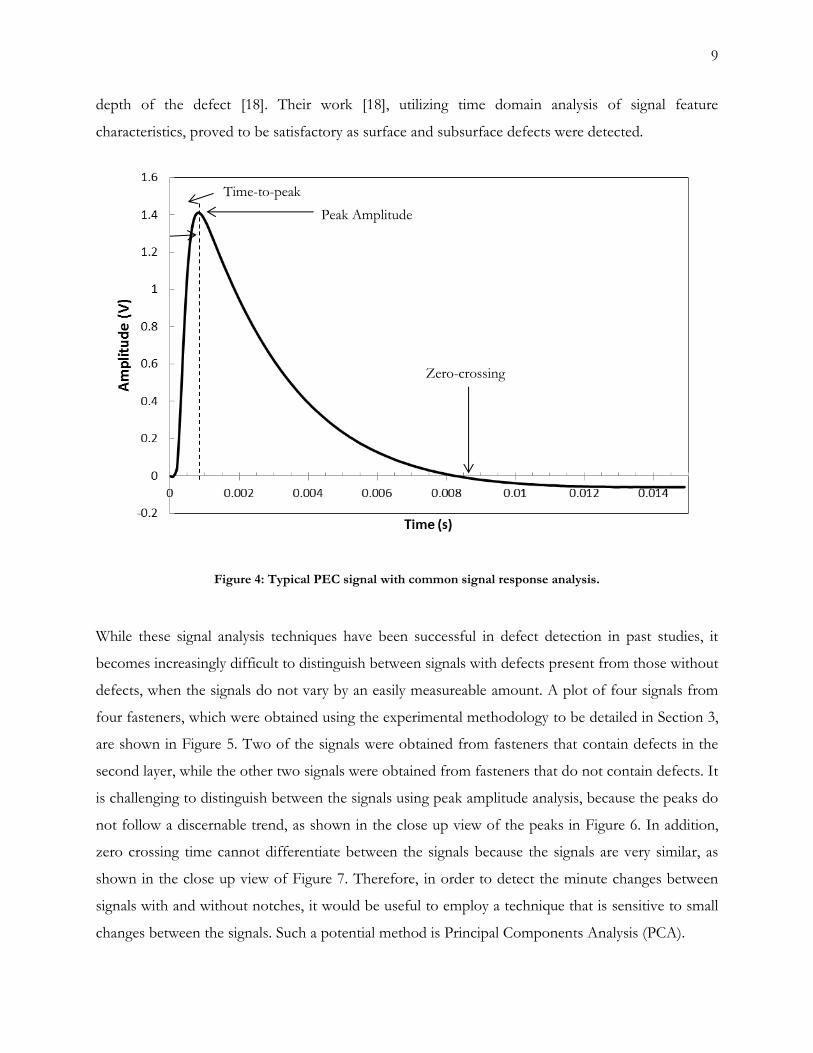
The response signals in PEC techniques provide information about the presence of potential

defects. Three commonly used methods of characterizing signals are shown below in Figure 4: time-

to-peak, peak amplitude and zero-crossing time [28]. Time-to-peak amplitude has provided defect

depth information in multi-layered structures [12]. He et al. [18] conducted experiments using

differential coils and Hall probes, showing that the peak amplitude of the response signal yields

information about the defect volume and that the zero crossing time yields information about the

Ferrite Core

Driving Coil

Ferrous Fastener

Pick-Up Coil

Conducting Plates

Crack

9

depth of the defect [18]. Their work [18], utilizing time domain analysis of signal feature

characteristics, proved to be satisfactory as surface and subsurface defects were detected.

Figure 4: Typical PEC signal with common signal response analysis.

While these signal analysis techniques have been successful in defect detection in past studies, it

becomes increasingly difficult to distinguish between signals with defects present from those without

defects, when the signals do not vary by an easily measureable amount. A plot of four signals from

four fasteners, which were obtained using the experimental methodology to be detailed in Section 3,

are shown in Figure 5. Two of the signals were obtained from fasteners that contain defects in the

second layer, while the other two signals were obtained from fasteners that do not contain defects. It

is challenging to distinguish between the signals using peak amplitude analysis, because the peaks do

not follow a discernable trend, as shown in the close up view of the peaks in Figure 6. In addition,

zero crossing time cannot differentiate between the signals because the signals are very similar, as

shown in the close up view of Figure 7. Therefore, in order to detect the minute changes between

signals with and without notches, it would be useful to employ a technique that is sensitive to small

changes between the signals. Such a potential method is Principal Components Analysis (PCA).

Peak Amplitude

Zero-crossing

time

Time-to-peak

10

Figure 5: Time domain response from four fasteners, with and without notches.

Figure 6: Zoomed view of peaks from Figure 5.

11

Figure 7: Zoomed view of zero-crossing from Figure 5.

1.3.4 PEC signals and Principal Components Analysis

Interpretation of the data gathered by PEC techniques can be used to characterize defects. However,

the time-domain signal characteristics of PEC are not amenable to the identification of small

differences in signals obtained in the presence and absence of cracks, as discussed above in Section

1.3.3. Advances have been made in the interpretation of the data by using modified PCA [16]. PCA

is a statistical technique that reorients highly correlated multivariate data so that the first few

dimensions account for as much of the available information as possible, making visualization of the

data more straightforward and subsequent data analysis more manageable [17]. PEC signals are

considered multivariate because the data contains more than one dependent variable [17]; i.e. the

signals are comprised of many sources of information such as the peak height, signal decay time and

zero-crossing points. Typical PEC analysis of aircraft components may produce multiple signals,

which contain between 100 and 1000 data points each. When data sets become unmanageable in

size, PCA can be used to compress the data into scores and vectors [17]. PCA scores can then be

investigated for correlation with a desired variable. In this thesis, the controlled dependent variable is

the presence of a defect. PCA has been applied in many different applications such as facial

recognition [29] and fault detection for semi-conductor manufacturing [30]. These multivariate

12

processes are not necessarily similar to PEC in theory, but are similar in the size of data set to be

analyzed and the correlated nature of the data.

Recent research using modified PCA techniques, [16] [27] [31] [32], concludes that PCA is an

effective method of analyzing results from a PEC probe. The traditional PCA uses an average signal

subtraction, whereas the modified version does not use this signal subtraction [16]. Recent work

using PCA has been performed by Horan et al. [16] [26] [27] and Underhill et al. [31] for crack

detection in CF-188 inner wing spars. A modified PCA method was used to identify signal variation

due to the presence of notches originating at fastener bore holes. The signals’ PCA scores, which are

based on the second and third eigenvectors of the PCA, provided the necessary discrimination to

separate signals when notches were present from signals obtained from no-defect sites [16].

FEM conducted elsewhere [32], utilized the probe design in this thesis work, which is shown in

Figure 8 and described in detail in Section 3.2. FEM investigated the effectiveness of PEC in

detecting deep lying cracks of different sizes and orientations in multi-layer aluminum structures,

utilizing PCA for signal analysis. The FEM simulated the response of a differential PEC probe to

top and bottom layer notches around a ferrous fastener. FEM demonstrated that PEC signals are

strongly influenced by the presence of an edge or slot, as shown in Figure 8, and by small probe

displacements, especially along the length of the crack. PCA was employed to reduce the signals to

scores and vectors, where the first and third scores yielded the clearest crack detection results [32].

13

Figure 8: Sample and probe geometry used in FE models [32].

1.3.5 PCA and Mahalanobis Distance

As stated previously in Section 1.3.4, discriminant analysis has been used to create separation

between PCA scores, obtained using the PEC technique, from fasteners with notches at their bore,

and fasteners without notches at their bore [27]. Scores from cracked (or notched) sites congregated

to one side of the cluster of scores from un-cracked sites. However, recent FEM [32] showed that,

in this thesis work, both crack orientation and size affects score position, i.e. scores from one crack

orientation will be rotated relative to scores from another crack orientation (in the multi-dimensional

score space) and discriminant analysis will not provide the necessary separation for detection of

cracks in multiple orientations. An alternative approach is to apply a quantitative measure of the

distance between groups, regardless of direction, to distinguish between cracks and non-cracks

(blanks). To accomplish this, a statistical technique called cluster analysis, specifically Mahalanobis

Distance (MD) analysis [17], is applied to the PCA scores. MD, which establishes the statistical

separation between sets of scores from similar objects, is used in conjunction with PCA to make the

distinction between signals with and without cracks more obvious. MD has been used in health

monitoring of electronic products [33], and also in combination with conventional eddy current

examination of nuclear fuel cladding for flaw indications [34], but has not presently been used to

interpret PCA scores for defect identification.

14

1.4 Objective

The aim of this thesis is to investigate the feasibility of pulsed eddy current technique to detect cyclic

fatigue cracking around ferrous fasteners in the second layer of lap joints. An 8-coil differential array

probe was used and the results analyzed using principal components analysis (PCA) and

Mahalanobis distance (MD) analysis. The CP-140 aircraft engineering office has determined that the

minimum detectable crack size in the lap-joint structure is 0.76 mm (0.03 in), in the transverse

direction [9].

1.5 Thesis Scope and Methodology

Section two presents the electromagnetic theory involved in the generation of eddy currents

followed by a description of the statistical theory pertaining to principal components analysis. Next,

the cluster analysis technique called Mahalanobis Distance is presented, as well as the Hotelling T2

threshold theory [35] for determining confidence intervals associated with crack detection.

Section three describes the experimental set-up. The first step is to describe the coil-based probe

design, and the sensing equipment set up. Next, the single fastener test piece and multiple fastener

test pieces are described in detail, including the material, crack lengths, orientations and locations.

Finally, the experimental procedures for each test piece case and the signal processing are explained

including the analysis method of signal gating.

Section four presents the results from the measurements conducted on the single fastener test piece,

and how the PCA scores are affected by off-centering the probe over the fastener, and by the

presence of a notch.

Section five presents the results of measurements taken on the three multiple fastener test pieces,

the NAVAIR sample, Test Piece #1 and CP-140-TT-1B. Effects on PCA scores due to off-

centering, presence of a notch, the height of the fastener head and lift-off, the effect due to the edge

of aluminum, and the effect due to fastener distance to the edge are presented. Next, the process

used for eigenvector selection is presented using logistic regression analysis. Finally, crack detection

results for the NAVAIR sample and test piece #1 are presented for both the absolute and

differential modes. Following this the results for the Aurora test piece (CP-140-TT-1B) are

presented in differential mode.

15

Section six discusses the performance of PEC technique combined with the PCA process for second

layer crack detection. A comparison with FEM is performed, and the similarities in results are

identified. Possible sources of uncertainty are also presented.

Section seven discusses the conclusions of this work, as well as recommendations for future work to

make this technique field-viable for second layer crack detection.

16

2 Theory

2.1 General

The aim of this Section is to first provide an overview of conventional and pulsed eddy current

inspection theories followed by a development of the physical principles for PEC inspection

techniques using electromagnetic theory. Maxwell’s Equations are presented to explain how

electromagnetic fields behave in conducting materials. Next, charge dissipation in a conductor will

be explained for pulsed eddy current techniques. The theory surrounding principal components

analysis is presented, followed by a derivation, as PCA is used to help reduce the signal data quantity

to a manageable amount. The output PCA scores are then used to calculate the Mahalanobis

Distance, which is compared to a decision threshold, based on reliability analysis, calculated using

the Hotelling T2 theory [35].

2.2 Maxwell’s Equations

In order to understand the principles behind eddy current inspection, the electromagnetic equations

describing this phenomenon must be examined. We begin with an outline of Maxwell’s four

Equations [10]:

(2.1)

(2.2)

(2.3)

(2.4)

where is the electric field, is the magnetic field, is the current density, is the charge density,

is the permittivity and is the permittivity and µo is the permeability, both of free space. Equation

2.1 is referred to as Gauss’s Law, equation 2.2 is referred to as Faraday’s Law, equation 2.3 indicates

17

that lines of flux are closed on themselves (no monopoles) and equation 2.4 is Ampere’s Law with

Maxwell’s correction.

Inside material, for linear and homogeneous media (uniform conductivity, permeability and

permittivity), the following relationships are valid [10]:

⁄

(2.5)

(2.6)

(2.7)

where is the magnetic field intensity and is related to the magnetic field by the permeability, μ. The

electric displacement, is related to the electric field by permittivity. Equation 2.7 is referred to as

Ohm’s Law, and is applicable in the conductors to be considered and states that the current density

is related to the electric field by the material’s conductivity (σ) [10]. Maxwell’s equations in matter

have the form [10]:

(2.8)

(2.9)

(2.10)

(2.11)

2.3 Electromagnetic Waves in Conductors

The flow of charge cannot be controlled within a conductor, and according to Ohm’s Law (equation

2.7), the current density is proportional to the electric field. Ampere’s law and Gauss’s Law are used

to derive the continuity equation, which by the Law of Conservation of Charge [10] (charge cannot

18

be created nor destroyed), states that the divergence of the current density is equal to the negative

rate of change of the charge density, and is expressed as [10]:

(2.12)

where is the free current density. Applying equations 2.7 and 2.8 to equation 2.12 yields [10]:

( )

(2.13)

For homogeneous linear media, a solution to equation 2.13 is [10]:

( ) ( )

(2.14)

Any free charge will dissipate in some characteristic time,

, meaning that any free charge on a

good conductor will flow out to the surface. For a perfect conductor, where conductivity is

effectively very large, . In good conducting materials (i.e. copper and aluminum), it is noted

that the characteristic time for free charges to dissipate is extremely fast, and is on the order of

[37], therefore, . This reduces equation 2.8 to .

2.4 Diffusion Equations

Next, the equations representing how electric and magnetic fields flow out of a conductor will be

derived. Applying the curl operator [10] to equation 2.9 yields:

( )

(2.15)

Using the following vector identity, where is an arbitrary vector [10]:

( ) ( )

(2.16)

One can apply equation 2.16 to equation 2.15 to yield:

( )

( )

(2.17)

19

Using the result from the previous section ( ), equation 2.11 can be substituted on the right

hand side of equation 2.17 to yield:

(

)

(2.18)

Rearranging, equation 2.18 becomes:

(2.19)

Equation 2.19 is Maxwell’s modified wave equation [10]. A similar solution can be obtained for the

magnetic field so that it is expressed independently of the electric field:

(2.20)

In good conductors, when the conductivity is very large, the following approximation can be used.

Copper has a conductivity of 5.8 x 107 siemens-m-1 [10], the multiplication of will be on the

order of 72.9, while the multiplication of , where is the radial frequency associated with the

changing fields, will be on the order of . The second term in equations 2.19 and

2.20 can be neglected because of the dominating first term, for frequencies less than approximately

108 Hz. A parabolic diffusion equation for the electric and magnetic fields remains [37]:

(2.21)

(2.22)

These two equations are similar to the equation for heat diffusion, and they express how the electric

and magnetic fields diffuse into the conductor.

20

2.5 Charge dissipation in a conductor

For an abruptly applied field (a pulsed field) Ohanian [37] suggests that in order to reach equilibrium

within the conductor, three steps must be achieved:

1. Expulsion of free charges,

2. Currents and dynamic electric and magnetic fields are expelled, and;

3. Surface currents and wave fields are damped.

Ohanian determined that a crude estimate of solutions to equation 2.22 would be [37]:

(2.23)

(2.24)

where l is the characteristic length. Combining these two equations with equation 2.22 yields [37]:

(2.25)

where τD is the characteristic diffusion time in seconds. The general solution to the diffusion

equation (equation 2.22) is of the form [13]:

(

⁄ ) (2.26)

The magnetic and electric fields will flow out of the volume of the conductor in some characteristic

diffusion time, which has a reasonable dependence on conductivity and permeability. Therefore, as

the conductivity increases, so will the diffusion time.

2.6 Skin Depth Theory

For the particular case of a surface coil above a thin conducting plane, Krause et al. [13] found that

equation 2.25 can be represented as:

(2.27)

21

where the square of the characteristic length from equation 2.26 has been substituted by T which is

the thickness of the plate, and D is a fit parameter connected to coil dimensions (diameter of the

ferrite core and also the pickup coil inner diameter).

A transient skin depth, denoted δ, can be inferred from equation 2.26 for a uniformly applied field

above a conducting half-space, and is represented as [13]:

√

(2.28)

Comparatively, the skin depth equation for conventional eddy current testing, in good conductors

(where μ>>ωε), is approximated as [10]:

√

(2.29)

2.7 Eddy Current Generation

The generation of eddy currents in electrically conductive materials is based on Faraday’s Law

(equation 2.9) where a changing magnetic field induces an electric field, or electromotive force (emf),

ε. Using the curl theorem [10], the emf can be expressed as:

∮ ∫

(2.30)

The magnetic field is related to the magnetic flux, , by the area integral ∫ [10].

Therefore, equation 2.30 can be expressed as:

(2.31)

The emf generated opposes the change in magnetic flux, denoted by the minus sign in equation 2.31,

also known as Lenz’s Law [10]. The changing magnetic flux induces eddy currents in the conductive

22

material, which are sensed via coils, and the net change in coil current or voltage is analyzed during

eddy current NDT.

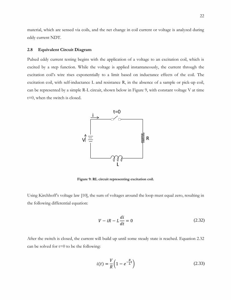
2.8 Equivalent Circuit Diagram

Pulsed eddy current testing begins with the application of a voltage to an excitation coil, which is

excited by a step function. While the voltage is applied instantaneously, the current through the

excitation coil’s wire rises exponentially to a limit based on inductance effects of the coil. The

excitation coil, with self-inductance L and resistance R, in the absence of a sample or pick-up coil,

can be represented by a simple R-L circuit, shown below in Figure 9, with constant voltage V at time

t=0, when the switch is closed.

Figure 9: RL circuit representing excitation coil.

Using Kirchhoff’s voltage law [10], the sum of voltages around the loop must equal zero, resulting in

the following differential equation:

(2.32)

After the switch is closed, the current will build up until some steady state is reached. Equation 2.32

can be solved for t=0 to be the following:

( )

(

) (2.33)

23

At t=0, the rise in current is almost instantaneous, and levels out at V/R, as shown in Figure 10.

This simple circuit representation shows the primary time dependence associated with the excitation

field involved in eddy current testing.

Figure 10: Current in driving coil representing equation 2.33.

To more closely model the actual experiment conducted in this thesis, a second coil (loop 2) may be

added to the circuit diagram, which is shown in Figure 11, and all the parameters are defined in

Table 1.

Table 1: Description of parameters for Figure 11.

Parameter Description

L1 Driving coil self-inductance

R1 Driving coil resistance

i1 Current through driving coil

M12 Mutual inductance

L2 Pick-up coil inductance

R2 Pick-up coil resistance

i2 Current in pick-up coil

Vo Input Voltage

24

Figure 11: Equivalent circuit diagram for driving coil and pick-up coil.

When the second circuit is introduced in proximity to the first, a mutual inductance coupling occurs

between them. Applying Kirchhoff’s Second Law to Figure 11 yields [38]:

( ) (2.34)

(2.35)

where all parameters are described in Table 1 and ( ) defines the step function. Applying the

Laplace transformation to equations 2.34 and 2.35, rearranging and solving those equations for the

current in loop 2 will yield [38]:

( ) (

)

( )( )

(2.36)

where the relaxation times are [38]:

Loop 1

Loop 2

25

( ) √( ) ( )

( )

(2.37)

The current response in the pick-up coil i2 is represented by the curve shown in Figure 12.

Figure 12: Current response in pick-up coil representing equation 2.36 (i2).

The system can be further characterized by adding a third circuit to represent the sample. The

mutual inductance relationships become inherently more complicated with the addition of the third

circuit, as shown in Figure 13, and in addition, boundary value solutions describing diffusion of

electric and magnetic fields into the sample, as expressed by equations 2.21 and 2.22, are required.

The mutual inductance equations are not solved in this thesis work.

26

Figure 13: Three-way mutual inductance relationships between driving coil, pick-up coil and sample.

2.9 Principal Components Analysis (PCA)

2.9.1 General

As described previously in Section 1.3.4, Principal Components Analysis (PCA) is a statistical

technique used to re-express multivariate data sets, thereby reducing their dimensionality, making it

inherently easier to identify patterns in the measured results, which maximize the explained

variation.

PCA can provide a means to determine the causes for variation within the signal such as: probe

misalignment over fastener, distance to edge of material, material thickness, varying fastener head

height, lift-off and presence of a defect. Notably, it is the presence of the defect that is most

important to this thesis work. Sophian et. al [39] have shown that PCA performed better than the

traditional methods of signal analysis for feature extraction such as peak height and arrival time.

2.9.2 PCA Method

The goal of PCA is to find a linear combination of the original data with the maximum variation

[17]. The modified PCA method uses a least-squares method of finding the best set of basis vectors

to represent the original signal, without average signal subtraction. Assume a data set is comprised of

multiple signal measurements containing the same number of data points, Y. Y can be represented

by a matrix with n rows (data points) and p columns (measurements), a column vector of which is Yi.

Ultimately, the aim of PCA is to find a column vector, v, that does the best job of representing a set

27

of p measurements with n data points, Y, in a least squares sense, where the column vector Yi can be

approximated by the column vector :

(2.38)

The goal is to choose a that minimizes the sum of squared residuals (denoted SSR) where:

∑∑( )

∑∑( )

∑∑

∑∑ ∑∑

(2.39)

The coefficient in equation 2.38 is referred to as the principal component score of a signal Y.

Next, it is assumed that v can be normalized by:

∑

(2.40)

The coefficient, , can be obtained by the scalar product of the transpose of Y and v to yield:

∑

(2.41)

where is the kth element of . Equation 2.41 can be expressed in matrix notation by:

(2.42)

Substituting equation 2.41 into the second term of equation 2.39 yields:

∑∑

∑ ∑∑

(2.43)

28

Applying the normalized condition of equation 2.40 to the last term in equation 2.43 reduces it to

∑

, therefore, equation 2.43 further reduces to:

∑∑

∑

(2.44)

In order to minimize the SSR, we must maximize the second term of equation 2.44. The second

term of equation 2.44, subject to the condition of equation 2.40, can be expressed as:

∑

(2.45)

This constrained optimization problem can be solved by forming the Lagrangian [17]:

( ) (2.46)

where λ is the Lagrange multiplier. Taking the derivative of equation 2.46 with respect to yields:

(2.47)

Setting equation 2.47 equal to zero and solving it yields the standard equation for eigenvectors and

eigenvalues [17]:

(2.48)

This shows that an eigenvector of will do the best possible job at representing the column

vectors in Y. It therefore shows that the eigenvector with the largest eigenvalue will describe more

of Y than any other vector. The vectors are uncorrelated, and a linear combination of only a few

eigenvectors will represent most of the variation in a larger data set.

Normally, the signal average is subtracted out of the matrix, before PCA is performed, as was done

by Sophian et. al [39]. The modified version of PCA does not use the average signal subtraction,

which makes it less sensitive to small changes in scale.

29

The benefit of PCA is that it only takes about four to five eigenvectors to represent 99.9% of the

original signal. In contrast, a Fourier series representation of the data would require a much larger

number of components to represent the data. Figure 14 below shows three curves, the first is an

unmodified pick-up coil signal or the original signal, the second is the first eigenvector

representation of the signal and the third is a reproduction of the original signal using the first four

eigenvectors. Note that 99.9% of the original signal is represented by the 1-4 eigenvector

reconstruction. The resulting scores from the PCA process describe the variation in the measured

PEC signals, including the presence of defects.

Figure 14: PEC original signal with first eigenvector reproduction, and eigenvectors 1-4 reproduction. The insert shows the four eigenvectors for each coil of the pair, used for the reproduction

2.9.3 PCA Scores

As mentioned above, the coefficients from the PCA process, , are termed the principal component

scores. The goal is to be able to use a few scores (1-5), instead of the 1000 data points per signal, to

determine whether or not a defect is present. Figure 15 (a) is a sample 3-D representation of the

second, third and fourth PCA scores, respectively, in the x, y and z axis, while (b) is a rotated view of

the same scores. The figures show scores from fasteners without notches (hollow circles) and scores

from notches of varying size and orientations (solid circles). It is difficult to discern from the view in

Figure 15 (a), which are the fasteners with notches present at their bore, as they tend to overlap.

30

Figure 15: PCA scores viewed in 3D, in the (a) un-rotated view and (b) rotated view for fasteners with (●) and without (○) notches at their bore.

Rotating the view of the PCA scores, which is shown in Figure 15 (b), the groups of scores tend to

cluster, showing separation between the groups of scores with notches from the groups of scores

without notches. Each cluster is correlated with notch size and orientation.

The figures presented above yield information about the presence of defects based on the amount

of separation between the groups. However, separation between clusters of scores does not always

occur, and groups can overlap regardless of the view in 3-D. This problem can be overcome by

using a cluster analysis, which will be described next in Section 2.10.

2.10 Cluster Analysis Method

2.10.1 Mahalanobis Distance Definition

A cluster analysis can be defined as organizing objects based on their similarities, where similar

objects are placed together, and dissimilar objects are placed apart [17]. One type of cluster analysis

is a distance measure called the Mahalanobis distance (MD). MD quantitatively describes the

proximity of a point, y, from the centroid of a group of points, while adjusting for covariance in the

data, and can be thought of as a measure of distance in standard deviations. MD can be calculated

by the following equation:

-0.75 -0.45 -0.15 0.15

S2

-0.10

-0.05

0

0.05

S3

-0.020

0.020.04

S4

-0.75-0.45

-0.150.15

S2

-0.10

-0.05

0

0.05

S3

-0.020

0.020.04

S4

Fasteners with

no-notch

(a) (b)

Fasteners with notch at bore

31

√( ̅) ( ̅) (2.49)

where ∑ is the covariance matrix of the data matrix X and ̅ is its centroid. In this case, the data

matrix consists of PCA scores obtained from signals without notches present. This covariance

matrix is then used to calculate MD for all available data (signals with notches and no-notch signals).

Therefore, in PCA space, MD is a relative or normalized measure of a notch’s distance from the

center of the cluster of blanks in standard deviations. MD is then compared to a critical value, or

decision threshold, in order to determine if the fastener has a notch or not. The requirement for a

decision threshold will be discussed in the next Section.

2.10.2 Decision Threshold

Separating PCA scores from fasteners with notches at their bore from those without requires a

threshold. Therefore, the MD2 for each fastener is compared to a critical value, the Hotelling T2 [35]

in order to assess the potential presence of a notch around a fastener. Values greater than T2 are

interpreted as cracks within the specified confidence interval. The following equation is used to

calculate the decision threshold:

( )( )

( ) ( ) (2.50)

where p is the number of PCA scores (S1, S2, etc), and n is the number of measurements used to

construct the covariance matrix, calculated by the number of blanks per test piece times the number

of measurements per fastener. Typically the F test, a statistical test which has an F distribution under

the null hypothesis [40], at either α = 99% or 95% confidence level, is used. The confidence level

gives the percentage of false positives that can be expected.

2.11 Probability of False Positive (False Calls)

A false positive, or false call (term used in this work is false call), is defined as a system response

interpreted as detecting a flaw when none is present at the inspection location [8]. It is difficult to

define what an acceptable false call rate would be for a specific technique, as the consequences of a

false call can be different depending on the type of inspection. For example, if the cost of a false

positive is high, then a very low false call rate is desired due to the amount of time and money

32

required to re-inspect the flaw site or remove the component from service. For this work, false calls

occur when a MD is calculated for a no-notch site that is greater than the specified threshold value.

The total amount of false calls is a sum of these events, divided by the total number of blanks in the

test piece.

33

3 Experimental Technique

3.1 General

This section begins by introducing the probe design used in this thesis. Next, the sensing equipment

used to conduct the experiments is described by use of a flow chart. Sample characteristics are then

described for the samples studied, which include: the single fastener test piece, the multiple fastener

test piece considered as the NAVAIR sample, the lab fabricated samples and the Aurora test piece.

The experimental technique utilized on these test pieces is then described. Finally, signal gating and

processing is explained.

3.2 Coil Probe Design

The probe configuration used in this thesis is based on designs examined in previous studies [2] [15]

[16], and incorporates the FEM discussed earlier in Section 1.1.1 [32] for optimization. The probe,

as shown in Figure 16, incorporates a central driving coil wound around a 6 mm diameter ferrite

core, chosen to match the head diameter of the fasteners. It has been determined that the magnetic

flux produced by the coil is magnified in the ferrite, and that it concentrates the magnetic field near

the center of the probe [23] [32]. This in turn concentrates the eddy currents near the center of the

probe and thereby generates a more sensitive response [2] in the pick-up coil configuration. The

orientation of the coil pairs, when placed on the aluminum, is indicated in Figure 16.

Figure 16: Probe face with central driving coil, ferrite core and eight pick-up coils.

The driving coil has 444 turns of 36 AWG wire. The driving coil and ferrite core are concentrically

located inside a probe body, which was printed on a 3-D printer. There are eight 1 mm high pick-up

Driving coil & ferrite core

Pick-up coils

270°

90°

0° 180°

34

coils of 400 turns of 44 AWG wire centered on 1 mm diameter ferrite cores, placed within 1.5 mm

of the outer diameter of the driving coil. The nearest-neighbor coil center-to-center distance is 5.6

mm. The pick-up coils are matched pairs placed 180° from one another on opposing sides of the

drive coil, approximately 14.2 mm apart (center-to-center distance) and may be connected in either

absolute or differential mode. In absolute mode, each coil is sampled individually, with eight

separate signals collected. In differential mode, the 180° coil pairs are sampled, but the difference in

their signals is collected. Therefore, in differential mode, only four signals are collected, one for each

coil pair. Eight coils were used so probe rotation is not required, facilitating notch detection in

multiple directions. Probe and coil information is located in Table 2. Coil-based sensing probes

detect the time rate of change of the magnetic field (refer to equation 2.31) produced by the eddy

currents in the aluminum.

Table 2: Driving coil and pick-up coil parameters.

Parameter Driving Coil with 6 mm ferrite core

Pick-up Coils

1 2 3 4 5 6 7 8

Resistance (Ω) 13.5 33.7 35.1 35.0 35.8 33.1 34.0 35.0 34.0

3.3 Sensing Equipment

The probe cable is connected via shielded twisted pair to a custom built amplifier board and the

amplified signal is digitized by a National Instruments (NI) 6361 data acquisition board at a group

rate of 100 kHz. A Labview program is used to control the pulse parameters. The pulse height and

width was 8.7 volts and 10 ms, respectively. Data from the pick-up coils was received through the

analog input on the NI card, and then transferred to the computer for storage. The experimental

process is depicted in the flow chart in Figure 17.

35

Figure 17: Flow chart depiction of sensing equipment operation cycle.

3.4 Single Fastener Test Piece

In order to understand the multiple fastener case, the single fastener case was studied because it

provides information concerning crack detection, without the complications of multiple fasteners,

crack sizes and orientations, and edge effects. Three 152 mm x 152 mm x 2.03 mm pieces of 2024-

T3 aluminum were stacked on top of each other. A hole was drilled in the middle of the stack, and a

ferrous fastener inserted to simulate an isolated fastener, as shown in Figure 18. There were three

experimental cases, which consisted of the middle plate either having a notch cut into the bore hole,

or no notch. The list of parameters for the experimental cases can be found in Table 3. It is noted

that the material in the middle plate is not always 2024-T3, however 7075-T6 is considered

electrically representative as shown in Table 3.

Figure 18: Side view of Single Fastener Test Piece with three plates and centrally located ferrous fastener.

Receives signal

Delivers pulse to driving coil

Pick-up signal sent to NI Card

Driving Coil

Pick-Up Coils

Induces eddy currents into AL wing skin

Computer NI Data

Acquisition Card

Triggers Pulse

Records signal

36

Table 3: Single fastener case experimental parameters.

Case # Material Notch Length (mm) Conductivity (%IACS)1

1 Al 2024-T3 No notch 30.0

2 Al 7075-T6 2 31.4

3 Al 7075-T6 8 31.4

3.5 Multiple Fastener Test Pieces

3.5.1 NAVAIR Sample Description

A sample (NAVAIR depot, Jacksonville Florida) has been acquired for testing purposes, and is

displayed in Figure 19 and Figure 20. The sample is based on the Lockheed P-3 Orion, which has

the same airframe as that of the CP-140 Aurora. It has overall dimensions of 54 cm × 28 cm with a

sheet thickness of 2.03 mm [32]. It consists of two separate sections of aluminum plates, which are

joined together by a row of ferrous fasteners in a lap joint where the two plates partly overlap, as

shown in the side view of Figure 20. Each fastener has a length of 15.0 mm, head diameter of 7.0

mm, shaft diameter of 4.54 mm, electrical conductivity of 3.57×106 S/m, and relative magnetic

permeability on the order of 70 [32].

1 http://www.ndt-ed.org/GeneralResources/MaterialProperties/ET/Conductivity_Al.pdf

Ferrous Fasteners

37

Figure 19: NAVAIR sample with notches, view from top.

Figure 20: NAVAIR sample with view of fastener.

The NAVAIR sample has electric discharge machined (EDM) notches located in 15 of the fastener

bore holes, and eight with no notches (8, 15, 16, 17, 18, 20, 22 and 23). Each notch is cut at a 45°

angle to the edge of the bore hole, giving the notch a 1:1 aspect ratio. The notch orientations are

based on the schematic shown in Figure 21. This sample contains fasteners with notches in the top

layer, bottom layer, and three that contain top and bottom layer notches. The notch lengths and

orientations are located in Table 4, where NN stands for no notch.

Figure 21: View from top. Notch orientation diagram.

A 135°

B 90°

E 270°

F 315°

C 45°

D 225°

0° 180°

Top Edge of Sample

38

Table 4: NAVAIR sample notch locations and lengths.

Fastener # Bottom-of-top

Layer Top-of-bottom

Layer Notch

Orientation Actual Notch Length (mm)

1 X A 3.30

2 X E 1.90

3 X D 1.78

4 X B 0.89

5 X C 5.46

6 X X F/F 3.30/0.89

7 X E 2.03

9 X D 1.52

10 X A 2.79

11 X B 0.89

12 X X C/D 5.46/3.30

13 X E 1.52

14 X F 5.08

19 X D 2.79

21 X X C/C 0.89/2.79

3.5.2 Test Piece #1 Description

Using the NAVAIR sample as a template, two test pieces were constructed in the lab. The test

pieces, fabricated of 2024-T3 aluminum, measure 61 cm × 13.2 cm with sheet thickness of 2.03 mm.

Twenty-nine holes of diameter 4.15 mm were drilled equidistant from each other (approximately

2.54 cm). Each fastener hole in the top layer was then countersunk 100° to a depth of 1 mm. The

fasteners tested in test piece #1 were ferrous fasteners of type HL-19-5-5. Each fastener was alloy

steel with a length of 8.0 mm, head diameter of 6.5 mm, and shaft diameter of 4.13 mm. The

technical information about these fasteners is located in Annex A.

For each fastener hole where a notch was to be cut, a set of Webber micro accurate gage blocks (in

millimeters) was used to accurately mark the notch length along the surface. Then, a jeweller’s saw

was used to cut notches into the bottom layer fastener holes at 45° angles, to the desired aspect ratio

of 1:1, as shown in Figure 21. The width of the blade was 0.3 mm for notch lengths above 0.9 mm,

and 0.17 mm for notch lengths below 0.9 mm. Afterward, notch lengths were measured to confirm

the actual length using a picture microscope (with Pixel Link software). A 3.12 mm (0.125 inch)

notch is shown in Figure 22, and the notch width was measured to be 0.38 mm. Notch orientations

reflect those of the NAVAIR sample, as shown in Figure 21. Figure 23 below shows test piece #1,

39

which has ten fasteners that have no notches in the bore (# 4, 5, 7, 10, 11, 12, 13, 20, 29), and 19

fasteners that have notches in the top of the bottom layer only. Additional information concerning

the parameters of test piece #1 such as notch orientation and actual notch length is shown in Table

5.

Figure 22: Microscopic photo of notch cut into fastener hole (11x magnification).

Figure 23: Picture of test piece #1.

40

Table 5: Test piece #1 notch parameters.

Fastener # Notch


2 D 1.97

3 A 1.17

6 B 1.94

8 F 1.46

9 C 1.43

14 E 3.20

15 B 3.26

16 B 1.97

17 E 1.92

18 E 0.82

19 A 1.46

21 B 2.03

22 F 1.24

23 E 0.94

24 D 1.36

25 A 1.51

26 A 1.80

27 F 2.81

28 F 0.83

3.5.3 Test Piece #2 Description

Test piece #2 was also fabricated in the lab, using the same technique as described above in Section

3.5.2. The test piece contains twenty-nine HL-19-5-5 fasteners, but does not contain any notches at

the fastener bore holes. This test piece was fabricated to assess effects such as height of fastener

head on PCA scores, lift off (probe above aluminum) and effect of fastener type without having the

scores affected by the presence of notches.

3.5.4 CP-140-TT-1B Test Piece

A wing skin section from a CP-140 Aurora was obtained from the Aerospace and

Telecommunications Engineering Support Squadron (ATESS). It has overall dimensions of 76.2 cm

× 20.5 cm × 3 cm with a top sheet thickness of 2.58 mm (considerably thicker than the NAVAIR

sample and Test piece #1) and a bottom sheet thickness of 2.29 mm. The sample has the same lap

joint construction as the NAVAIR sample mentioned in Section 3.5.1, and is shown in Figure 24.

The fasteners are of type HLT-51-6, with head diameter of approximately 7.5 mm and shaft

41

diameter of 4.8 mm, as per fastener specs in Annex B. The sample has EDM notches located in 21

of the fastener bore holes, and 12 with no notches (1, 2, 3, 4, 8, 12, 14, 22, 30-33). Notches can be

located in either top-of-bottom layer or bottom-of-top layer. Notch orientations are similar to those

outlined in Figure 21. However, for this sample, notch orientations and lengths are presented in

more detail in Table 6. For fasteners that contain multiple notches at their bore, a numbering system

is used (such as fasteners 16, 17, 18, 19, 21 and 28), indicated by an additional bracketed number.

For fasteners that contain notches at their bore with irregular orientations (such as fasteners 9 and

19), a lettering system is used, and schematics of these notches are shown in Figure 25.

Figure 24: Picture of section of CP-140-TT-1B test piece.

Figure 25: Schematics of notches located at fasteners 9 and 19 of CP-140-TT-1B Aurora Sample.

42

Table 6: CP-140-TT-1B notch parameters.

Fastener # Bottom-of-top

Layer Top-of-bottom

Layer Notch


5 X 315° 2.54

6 X 180° 3.30

7 X 60° 1.53

9a X 270° 0.20

9b X 315° from 9a 2.54

10 X 45° 3.81

11 X 105° 2.92

13 X 60° 1.72

15 X 0° 3.30

16 (1) X 180° 2.03

16 (2) X 90° 3.81

17 (1) X 270° Unknown

17 (2) X 180° 2.03

18 (1) X 315° 2.03

18 (2) X 45° 2.03

19 (1) X 270° 2.54

19 (2a) X 330° 2.03

19 (2b) X 30° from 19 (2a) 2.54

20 X 255° 2.54

21 (1) X 270° 2.54

21 (2) X 90° 2.54

23 X 75° 2.54

24 X 315° Unknown

25 X 240° 2.92

26 X 60° 3.81

27 X 300° 1.53

28 (1) X 300° 1.53

28 (2) X 60° 1.53

29 X 105° 2.03

3.6 Experimental Procedure

3.6.1 Probe Alignment

Alignment of the probe over the fastener is achieved with an acrylic alignment guide, shown in

Figure 26. The alignment tool has a thin clear sheet with a center hole the same size as fastener head,

which is used to align the probe over the fastener head. The alignment tool, probe and sample are

43

shown in Figure 27. For each measurement, alignment of the probe’s 0th position occurs along the

row of fasteners, subsequently, the other coil pairs will then be aligned over the potential crack

propagation directions. For each individual measurement, the alignment tool was removed and

replaced over the fastener. This process is achieved by eye, as to best represent the actual inspection

technique performed by an NDT technician. Centering errors can occur on the order of

approximately 1-2 mm utilizing this technique. During laboratory experiments, multiple

measurements are taken at each fastener. This ensures that variability due to probe placement is

properly represented in the data set.

Figure 26: Alignment tool, showing the direction of shimming (0° and 90°).

0°

90°

270°

180°

45° 135°

225° 315°

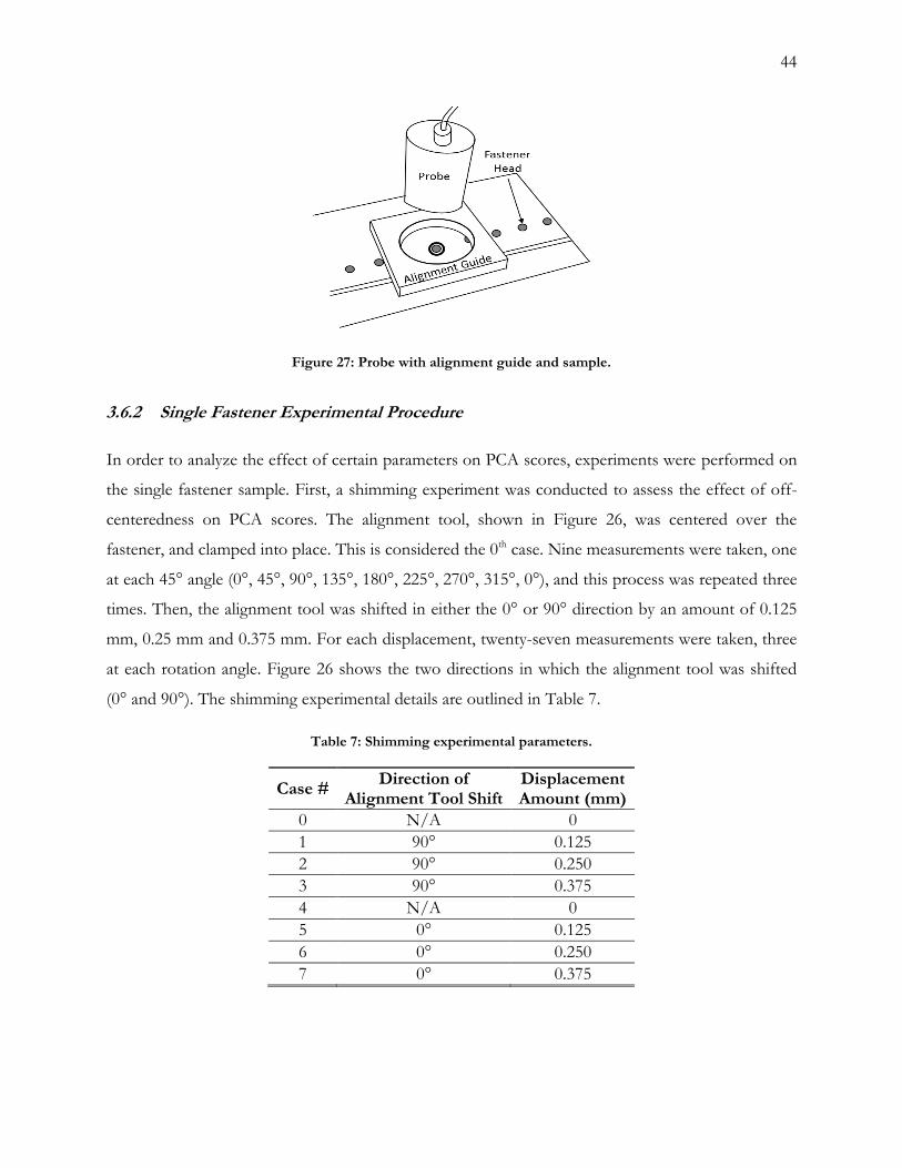
44

Figure 27: Probe with alignment guide and sample.

3.6.2 Single Fastener Experimental Procedure

In order to analyze the effect of certain parameters on PCA scores, experiments were performed on

the single fastener sample. First, a shimming experiment was conducted to assess the effect of off-

centeredness on PCA scores. The alignment tool, shown in Figure 26, was centered over the

fastener, and clamped into place. This is considered the 0th case. Nine measurements were taken, one

at each 45° angle (0°, 45°, 90°, 135°, 180°, 225°, 270°, 315°, 0°), and this process was repeated three

times. Then, the alignment tool was shifted in either the 0° or 90° direction by an amount of 0.125

mm, 0.25 mm and 0.375 mm. For each displacement, twenty-seven measurements were taken, three

at each rotation angle. Figure 26 shows the two directions in which the alignment tool was shifted

(0° and 90°). The shimming experimental details are outlined in Table 7.

Table 7: Shimming experimental parameters.

Case # Direction of

Alignment Tool Shift Displacement Amount (mm)

0 N/A 0

1 90° 0.125

2 90° 0.250

3 90° 0.375

4 N/A 0

5 0° 0.125

6 0° 0.250

7 0° 0.375

45

3.6.3 Multiple Fastener Test Piece Experimental Procedure

Alignment of the probe over the fastener is achieved using the procedure outlined in Section 3.6.1,

for each of the four multiple fastener test pieces. The number of measurements obtained per

fastener varied between test pieces, and is detailed in Table 8. As mentioned previously, multiple

measurements were taken to assess variability due to probe placement, but were also used to assess

repeatability of measurements.

Table 8: Number of measurements taken per test piece.

Number of Measurements/Fastener

Test piece Absolute Differential

NAVAIR 10 10

Test Piece #1 2 2

Test Piece #2 10 0

CP-140-TT-1B 0 4

3.7 Summary of Experiments

Table 9 below summarizes the tests conducted on each test piece. The results of these experiments

will be presented in Sections 4 and 5.

Table 9: Summary table of experiments conducted on each test piece, in sequence.

Test Sequence

Specimen Probe Off-

Centeredness Notch

Presence of Edge

Distance to Edge

Fastener Head

Height

Lift-Off

Effect of Temperature

1 Single

Fastener Test Piece

X X

2 Test Piece

#1 X X

3 Test Piece

#2 X X

4 NAVAIR Sample

X X X

5 CP-140-TT-1B

X X

46

3.8 Signal Processing

3.8.1 Signal Gating

Analyzing the whole signal is not appropriate for PEC responses, when PCA will be applied. Figure

28 shows a PEC signal from a fastener without a notch present. Previous experience indicates that

including the rapidly changing signal between 0 and 0.00058 seconds causes the PCA to concentrate

on representing the large variations in the signal that this induces. The virtually exponential decay of

the signal means that there is almost no signal to analyze after 0.0015 seconds [32]. Precise

determination of where the notch information is contained is difficult to achieve. The modeling

reveals that the highest concentration of eddy currents, greater than 90%, occurs near the flaw site

between 0.0004 and 0.001 seconds, as shown in Figure 29. For the purposes of this thesis, the signal

“gating” [26] occurs from 0.00058 to 0.0015 seconds, in order to encompass the portion of the

signal with the greatest amount of crack detection information.

Figure 28: Raw PEC data signal from a fastener without a notch, indicating the gate.

Signal Gate

47

Figure 29: Eddy current density curve from finite element modeling.2

3.8.2 Signal Analysis

The modified PCA process is applied to the windowed data described in Section 3.8.1 using a

Labview program. For differential analysis, the PCA scores are calculated for each of the four signals

separately. The coil pairs were analyzed individually because they are not identical, and, therefore,

the eigenvectors describing their response are expected to be slightly different. In absolute mode,

each of the eight coils produces a response signal. The 180° coil pair signals are selected,

concatenated, gated and PCA is applied to the gated data. In differential mode, four signals are

produced (one for each coil pair). Therefore concatenation of the coil pairs is not necessary. The

outcome of this process is a set of PCA scores for each fastener. Once the scores are obtained, the

centroid and covariance matrix for the signals from blanks was determined for each coil pair. The

Mahalanobis distance was then calculated for each fastener, by coil pair, using equation 2.49. The

distance calculations were done on a per coil pair basis because coil pairs are not completely

equivalent and so the response from each pair to a crack can be expected to be different. In

addition, because the probe had a set orientation, each coil pair can be expected to have different

sensitivity to a crack depending on both the crack’s relative orientation to the probe and its relative

orientation to the lap joint.

2 FEM Courtesy of Dr. Vijay Babbar, Department of Physics, Royal Military College of Canada, Kingston, Ontario

48

The Mahalanobis Distance for each fastener is then compared to the threshold value, calculated

using equation 2.50. Fasteners with a distance greater than the threshold are considered as having a

notch present, and those below are considered blank. The results from each coil pair for each

fastener were then logically ORed, i.e. a positive for one coil pair counted as a crack detected for

that fastener. The data processing sequence is outlined in Figure 30.

Figure 30: Data processing sequence for PEC signals.

Pick-up coil response

Signal Gated Eigenvector

Multiplication with signal

PCA Scores Procuded

Mahalanobis Distance

Calculated

Mahalanobis Distance

Compared against threshold value

49

4 Results and Analysis of Single Fastener Case

4.1 General

This section discusses the results obtained from the single fastener test piece, and the PCA score

correlation with different variables, such as off-centering, and the presence of a notch. It is desirable

to isolate the different effects on the PCA scores by varying one parameter while holding the others

fixed so that the most appropriate scores for notch/crack detection may be identified.

4.2 Off-Centering Effects

After collecting and recording the data in differential mode, for the cases outlined in Table 7, the

PCA scores were calculated for each coil pair. The FEM [32] indicated that misalignment of the

probe over the fastener head affects the PCA scores S1 and S2, the greater the displacement, the

larger the PCA score becomes. In order to assess the effect of misaligning the probe over the

fastener, the PCA scores were plotted against each other, in different combinations. Figure 31 is a

plot of the first and second PCA scores for the single fastener with no notch present for the

centered case, and for probe displacement cases of 0.125 mm, 0.250 mm and 0.375 mm. The

displacement direction is indicated in each figure, and the arrows indicate the direction of increasing

off-centeredness. Displacing the probe from the centered position causes PCA score S1 to become

larger, as indicated by the positive horizontal shift of the points in Figure 31. Displacement of the

probe over the fastener does not cause any effect on the second PCA score (S2), as there is no shift

in the amplitude of the vertical axis.

Figure 31: Plot of PCA scores S2 versus S1 for single fastener with no notch, showing off-centered results.

50

Figure 32 is a plot of the same test conducted as outlined in Table 7, but is a plot of the first and

third PCA scores (S1 and S3). It is shown that similar to the second PCA score, the third score (S3)

does not contain off-centering information, because there is no shift in the vertical axis direction as

the probe center is shifted relative to the center of the fastener head. In addition, the fourth and

fifth PCA scores are plotted in Figure 33, where the amplitude change in the horizontal and vertical

axes is very small. Therefore, there is a minor effect of off-centering on the fourth and fifth PCA

scores (1% and 3% of S1, respectively).


51


4.3 Notch Effects

Another correlation to be studied using PCA on PEC signals is the presence of a notch. Above in

Section 4.2, the off-centering correlation is with PCA scores S1, S4 and S5, with no correlation with

scores S2 and S3. These results stem from experiments conducted for three cases; the no-notch, 2

mm and 8 mm cases. The notches were through notches and located in the second layer, which was

under 2 mm thick aluminum (see Section 3.4 for more detail). In addition, the notches were aligned

with 0° (see Figure 26 for alignment reference). In Figure 34, the first and second PCA scores are

plotted for the centered probe over the fastener for the three cases, where the arrows indicate

direction of increasing notch length. In both the horizontal and vertical directions, the score values

increase either positively or negatively due to the presence of the notch. In Figure 35, the second

and third PCA scores are plotted for the same three cases. The effect on the second PCA score is

larger than the effect on the third PCA score, but there still seems to be an effect, although minor,

on S3 due to the presence of a crack. Figure 36 is a plot of the fourth and fifth PCA scores, which

shows an effect on the fourth but not the fifth score due to the presence of a crack. Therefore, the

first, second, third and fourth PCA scores show effects due to the presence of a crack in the second

layer for the single fastener case.

52

Figure 34: Plot of PCA scores S2 versus S1 for single fastener case of no notch (⟡), 2 mm (⧠) and 8 mm (∆) notch. Arrows indicate direction of increasing notch length.


53


Off centering and presence of a notch were the only two effects that were analysed for the single

fastener test piece. These results demonstrate correlation of PCA scores with off-centeredness and

presence/absence of a notch. In order to understand how other factors such as fastener head height,

presence of the edge and lift-off affect the PCA scores, the multi-fastener test pieces were

investigated next.

54

5 Results and Analysis of Multiple Fastener Case

5.1 General

This section describes the effect on the PCA scores due to off-centering, presence of a notch, height

of the fastener head and lift off, presence and distance of fastener from the edge. Second, the

process used for eigenvector selection is presented using logistic regression analysis. Third, crack

detection results for the NAVAIR sample and test piece #1 are presented for both the absolute and

differential modes. Fourth, the results for the Aurora test piece (CP-140-TT-1B) are presented for

only the differential mode.

5.2 Off-Centering Effects

The off-centering effects for the single fastener test piece were presented above in Section 4.2,

where PCA score S1 showed the biggest effect due to displacement of the probe. To confirm that

the same effects occurred on the multiple fastener test pieces, seven experiments were conducted

between two separate fasteners on the NAVAIR sample. These were fastener 1, which contained a

3.3 mm notch at 315° in the second layer, and fastener 22, no notch present. The seven experiments

are outlined in Table 10, and displacement directions are outlined in Figure 26 .

Table 10: NAVAIR sample experimental cases for off-centering and notch effects on PCA scores.

Case # Fastener Notch

Length (mm) Displacement Amount (mm)

Displacement Direction

1 22 0 0 Nil

2 22 0 0.125 90°

3 22 0 0.250 90°

4 22 0 0.125 180°

5 22 0 0.250 180°

6 1 3.3 @ 315° 0 Nil

7 1 3.3 @ 315° 0.375 90°

Figure 37 is a plot of the first and second PCA scores (S1 and S2), from the 0° coil pair, for the

experiments outlined in Table 10. It is observable on this graph in points 2-5, that displacing the

probe away from the centered position (point 1, no notch present) has a large effect on the first

PCA score S1, and only a very minor effect on S2. In addition, there seems to be a minor effect on

the third, and fifth scores (S3 and S5) shown in Figure 38 and Figure 40, and no effect on the fourth

score, shown in Figure 39. As stated previously, off-centering was correlated the most with S1 in the

55

single fastener case, with a weaker correlation with S4 and S5. For the multiple fastener case, off-

centering effects are correlated the most with S1, and a weaker correlation was observed for S2, S3

and S5. Since the biggest effect is shown on the first score, the results are consistent with the single

fastener case. The fact that more correlation with PCA scores was shown on the multiple fastener

test piece can be attributed to effects due to adjacent fasteners or the presence of the edge.

Figure 37: Plot of S2 versus S1. Numbers correspond to Table 10 cases. For probe displacement (disp), arrows indicate direction of increasing displacement.

56



57


5.3 Notch Effects

Again, considering the results of the single fastener case presented in Section 4.3, the presence of a

notch tended to correlate with the first and second scores, with minor correlation with the third and

fourth PCA scores. Considering point number 6 in Figure 37, which was measured for a 3.3 mm

notch with no displacement, correlation is observed with the first score S1, and a weaker correlation

with the second (S2). For the same point (6) in Figure 38, there is an observed correlation with PCA

score S3 due to the presence of a notch, while in Figure 39 and Figure 40, there is a weak correlation

with S4 and S5. Clearly there are similarities between the single fastener case and the multiple

fastener case, but the differences may be attributed to the presence of adjacent fasteners or the

presence of the edge.

5.4 Effect Due to Height of Fastener Head and Lift-Off

Additional variables affecting the transient response are the height of fastener head relative to the

aluminum surface, and the height of the probe above the aluminum surface, considered as lift-off.

Results from the investigation of effect of height of fastener head relative to the aluminum surface

58

are presented in the next section. Subsequently, effects due to lift-off are then presented in Section

5.4.2.

5.4.1 Fastener Head Height Effects

While this variable is not a large factor on actual aircraft, since fastener holes are countersunk with

high precision, it was a factor in lab settings, as it is challenging to countersink fastener heads with a

high degree of accuracy, while fabricating test pieces (Test piece #1 and #2). The height of the

fastener heads relative to the aluminum was measured on Test Piece #2 using a depth measuring

device. This information is available in Table 11, where a negative number means the fastener head

is below the aluminum surface, and a positive number means it is above. All fastener holes in this

test piece do not have notches.

Table 11: Test Piece #2 HL-19-5-5 fastener head height relative to aluminum surface, for no notch sites.

Fastener # Fastener Height (mm)

Fastener # Fastener Height (mm)

9 0.29 6, 7, 29 0.01

1 0.255 17 -0.01

2, 5 0.23 19 -0.04

8 0.22 20, 27 -0.05

12 0.21 23 -0.13

3 0.20 28 -0.14

10, 11 0.17 18 -0.15

4 0.15 21 -0.19

13, 14, 22 0.05 25 -0.2

16 0.03 24 -0.21

15 0.02 26 -0.23

The experiment consisted of ten measurements on each of the twenty-nine fasteners in Test Piece

#2. Figure 41 shows the plot of S1 versus fastener head height in millimeters, where it can be shown

that as the fastener head rises above the aluminum surface, there is a slight decline in the size of the

PCA score S1. Figure 42 shows the correlation of fastener head height relative to aluminum with

PCA score S2. As the fastener head rises above the aluminum surface, the S2 score decreases.

Figure 43 shows the plot of fastener head height relative to aluminum with the third PCA score. No

correlation is observed with fastener head height and S3. The lack of correlation with fastener head

59

height and S3 is an important observation; recall Section 4.3, the presence of a notch is indicated on

PCA score S3. Figure 44 and Figure 45 show similar relationships between fastener head height and

S4 and S5, respectively, where it is observed that there is no effect of changing fastener head height

on the amplitude of the fourth and fifth PCA scores.

Figure 41: Effect of fastener head height distance and lift-off distance on first PCA score (S1).

Figure 42: Effect of fastener head height distance and lift-off distance on second PCA score (S2).

60

Figure 43: Effect of fastener head height distance and lift-off distance on the third PCA score (S3).

Figure 44: Effect of fastener head height distance and lift-off distance on the fourth PCA score (S4).

61

Figure 45: Effect of fastener head height distance and lift-off distance on the fifth PCA score (S5).

Following these experiments and subsequent data analysis, a new top piece for each of test piece #1

and #2 were fabricated with a more precise countersink operation, due to the large effect of fastener

head height on PCA scores. This was completed to better simulate actual wing structures and reduce

the effect due to varying fastener head height on measured results.

5.4.2 Lift-off Effects

Another variable assessed was probe lift-off above the fastener in the aluminum. Test piece #2 was

used to conduct this experiment, where six measurements were taken on fasteners 24, 25 and 26,

and their starting head heights were -0.2, -0.21 and -0.23, respectively. Starting at zero lift-off, a shim

of thickness 0.10 mm was added under the probe so as to raise it above the aluminum. A total of

five shims were added under the probe, raising it a total of 0.5 mm above the aluminum. The six

points from the lift-off experimental results are plotted above in Figure 41. A linear trendline was fit

through the data that shows a positive linear effect on the first PCA score as the probe is raised

above the aluminum. Figure 42 above also shows the effect of lift-off on the second PCA score. A

linear trendline that was fit through the data shows a positive linear trend on the second score with

increasing lift-off. Figure 43 above shows the plot of the third PCA score with lift-off, where the

trendline through the S3 data has a slope value of zero, so there is no correlation of lift-off with the

third score as the probe is raised above the aluminum surface. Furthermore, Figure 44 above is a

plot of the fourth PCA score with lift-off and there is a slight negative slope to the trend-line

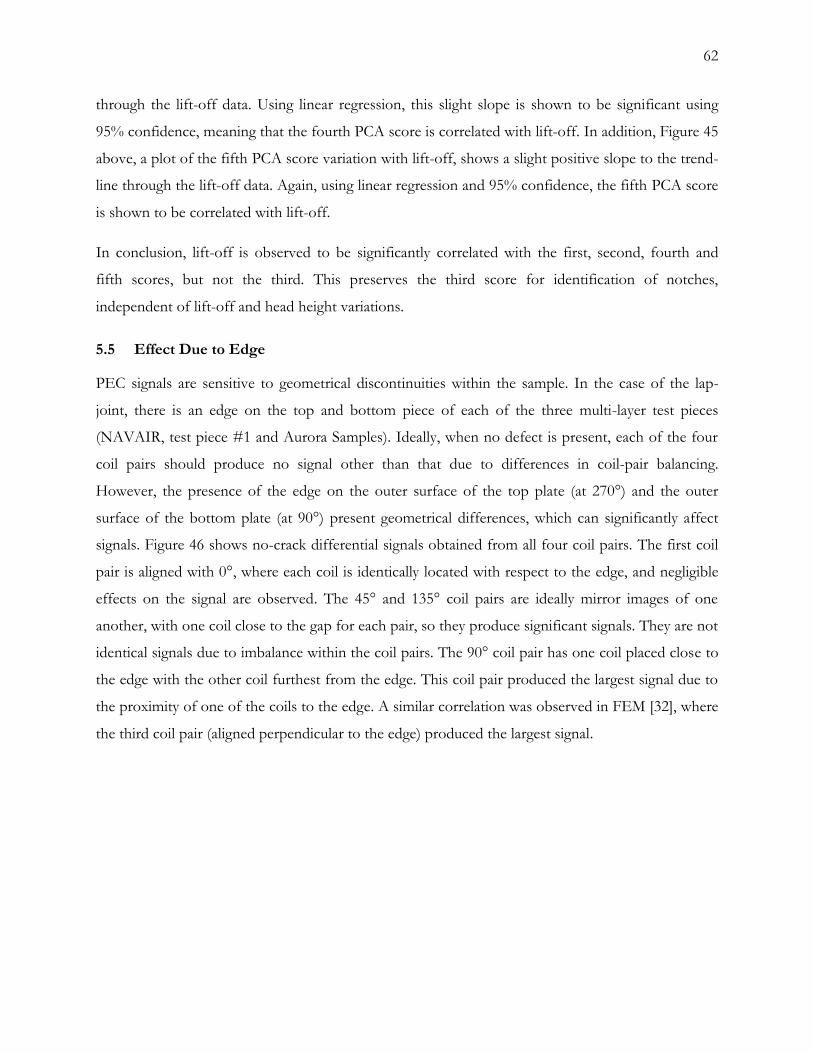
62

through the lift-off data. Using linear regression, this slight slope is shown to be significant using

95% confidence, meaning that the fourth PCA score is correlated with lift-off. In addition, Figure 45

above, a plot of the fifth PCA score variation with lift-off, shows a slight positive slope to the trend-

line through the lift-off data. Again, using linear regression and 95% confidence, the fifth PCA score

is shown to be correlated with lift-off.

In conclusion, lift-off is observed to be significantly correlated with the first, second, fourth and

fifth scores, but not the third. This preserves the third score for identification of notches,

independent of lift-off and head height variations.

5.5 Effect Due to Edge

PEC signals are sensitive to geometrical discontinuities within the sample. In the case of the lap-

joint, there is an edge on the top and bottom piece of each of the three multi-layer test pieces

(NAVAIR, test piece #1 and Aurora Samples). Ideally, when no defect is present, each of the four

coil pairs should produce no signal other than that due to differences in coil-pair balancing.

However, the presence of the edge on the outer surface of the top plate (at 270°) and the outer

surface of the bottom plate (at 90°) present geometrical differences, which can significantly affect

signals. Figure 46 shows no-crack differential signals obtained from all four coil pairs. The first coil

pair is aligned with 0°, where each coil is identically located with respect to the edge, and negligible

effects on the signal are observed. The 45° and 135° coil pairs are ideally mirror images of one

another, with one coil close to the gap for each pair, so they produce significant signals. They are not

identical signals due to imbalance within the coil pairs. The 90° coil pair has one coil placed close to

the edge with the other coil furthest from the edge. This coil pair produced the largest signal due to

the proximity of one of the coils to the edge. A similar correlation was observed in FEM [32], where

the third coil pair (aligned perpendicular to the edge) produced the largest signal.

63

Figure 46: Experimental no-crack differential signals from all four coil pairs.

5.6 Effect Due to Fastener Distance from Edge

Section 5.5 showed how the coil pair signals are affected by the presence of the edge. This result

suggests an investigation into the effect of fastener distance from the edge, should be performed.

Some variability in fastener distance to the edge of the aluminum is observed on actual aircraft

structures, possibly since these were manually located. The distance from the edge of the fastener to

the edge of aluminum was measured on no-notch fasteners (1, 2, 3, 4, 30, 31, 32, and 33) on the CP-

140-TT-1B Aurora sample, and these distances are presented in Table 12.

Table 12: Distance from edge of fastener to edge of aluminum.

Fastener # Distance to Edge (mm)

30 6.21

33 6.34

2 6.44

31 6.50

32 6.68

1 6.72

3 6.99

4 7.05

64

PCA scores obtained from measurements taken on the Aurora sample were examined for each coil

pair. For the 90° coil pair, which showed the biggest effect due to the edge as presented in Section

5.5, the first, second and third PCA scores showed negligible correlation with fastener distance to

edge. The fourth and fifth scores were plotted with distance from the fastener edge to the edge of

aluminum and are shown in Figure 47 and Figure 48, respectively. There is an observed correlation

with fastener distance to the edge of aluminum and PCA scores S4 and S5. Since the presence of a

notch is correlated most strongly with the third PCA score, and a weaker, but significant correlation

is observed on the fourth and fifth scores, the effect due to the edge is expected to have only a

minor effect on notch detection capability.

Figure 47: PCA score S4 plotted with fastener distance to edge in millimeters.

Figure 48: PCA score S5 plotted with fastener distance to edge in millimeters.

65

5.7 Effect of Temperature on Probe Performance

A separate group of tests was conducted on Test Piece #1 to assess the possible effect of

temperature on probe functionality. Six fasteners, that do not contain notches at their bore, were

tested in a temperature controlled chamber, where the probe and sample was conditioned to three

temperature settings (9°, 20° and 30° Celsius). There was no observed effect on the first three PCA

scores, and the results of these tests are presented in Annex C.

5.8 Results on NAVAIR Sample

5.8.1 Test Piece Summary

The NAVAIR sample contains EDM notches in the bore holes of 15 out of 23 fastener locations.

The top layer thickness is 2 mm. The fasteners are of type HL-19 and have a head diameter of 7

mm. The notches range in length from 0.89 to 5.46 mm and are located in both the top-of-bottom

layer and bottom-of-top layer.

5.8.2 Eigenvector Selection

The first five eigenvectors for the third coil pair, resulting from differential mode analysis on the

NAVAIR sample, are shown in Figure 49. The first vector represents an average of all the data that

went into the analysis, and the subsequent vectors account for the observed variation. As stated in

Section 2, only the first few eigenvectors are required to accurately reproduce the original signal as

represented by the residual sum of squares calculated between the original and reproduced data. In

this thesis work, five eigenvectors are used to reproduce the original signal for three reasons. First,

Figure 50 shows the results obtained from logistic regression [17] to the hit/miss data on second

layer cracks obtained when the scores of 1-3, 1-4 and 1-5 eigenvectors are used to calculate the

Mahalanobis distance. A 99% confidence level was used to calculate the Hotelling T2 value. From

this figure it can be seen that using four eigenvectors (a50 = 1.55 mm) rather than three (a50 = 2.35

mm) improved the detectability for smaller cracks, but offers little improvement at larger crack sizes.

On the other hand, using five eigenvectors (a50 = 0.90 mm), the whole curve shifts significantly to

the left. Therefore, using five eigenvectors rather than three or four, gives substantially better crack

detection.

Second, FEM [32] suggested that the highest concentration of eddy currents occurs between 0.0004

- 0.001 seconds (see Figure 29). The fourth and fifth eigenvectors, shown in Figure 49, reach peak

66

amplitude in the same timeframe where eddy currents are the strongest in the second layer. The

correlation of eigenvector peak amplitude with higher current density is consistent with the

observation of improved detectability, as shown in Figure 50.

Finally, the signal-to-noise ratio of the eigenvectors severely degrades past the fifth vector, making it

ineffective to reliably use more than five vectors for signal analysis.

Figure 49: First five eigenvectors of PCA on data from NAVAIR third coil pair (differential mode).

67

Figure 50: Results from logistic regression performed on hit miss data from NAVAIR sample using 1-3, 1-4 and 1-5 eigenvectors. Horizontal axis is on a log scale.

5.8.3 Absolute Mode Crack Detection Test Results

The experimental process described in Section 3.6.3 was performed on the NAVAIR sample using

the probe in absolute mode. After data collection, the PCA process was applied to the signals. The

first step is to gate the signal at the appropriate time where defect information is believed to be

located. With coils in absolute mode, the eight coil pairs output eight individual signals. The signals

corresponding to coil pairs 180° from one another are selected, concatenated and gated in the same

time interval. PCA is conducted on each coil pair separately and once completed the scores are

available to be examined.

The PCA scores from four fasteners with notches and four fasteners without notches are shown in

Figure 51. The solid filled circles, squares and triangles are scores from fasteners with notches at

their bore. The hollow circles are scores from fasteners with no notches at their bore. The group of

scores in black circles are scores from the smallest notch (0.89 mm). There is overlap between this

group and the group of blanks. This poses a problem for crack detection, as the notches can be

disguised as blanks in PCA space, as stated previously in Section 2.9.3.

68

Figure 51: 3-D view of NAVAIR data PCA scores S2, 3 & 4.

In order to better distinguish between notches and blanks, the Mahalanobis Distance is calculated

for each fastener. It is apparent from Figure 51 that PCA scores S2, S3 and S4 could be used to

calculate the MD, as they appear to provide good separation for some fasteners with notches.

However, five scores (S1-S5) are used to calculate the MD as some information is also located in S1

and S5 as discussed earlier in Section 5.8.2. Using scores S1-S5 increases crack detection and lowers

false call rates. The MD is then compared to the threshold, calculated using equation 2.50. The

threshold calculated for this experiment was 4.2 at 99% confidence and 3.5 for 95% confidence.

There are no units associated with the MD, as it is a relative measure of distance from the centroid

of the cluster of blanks, in terms of standard deviations. The MD was plotted for each fastener and

the plot is shown in Figure 52, along with the decision thresholds, while results of this test are

shown in Table 13. It is worth noting that the MD associated with fasteners 5 and 14 corresponds to

the biggest second layer notches, at 5.46 mm and 5.08 mm, respectively. As the notches decrease in

size, so does the MD as indicated by MD values for fasteners 4 and 11. This indicates that there is a

correlation of MD with notch size, which will be investigated further in Section 5.8.5.

-0.8

-0.6

-0.4

-0.2

0

0.2

S2

-0.04-0.02

00.02

0.04

S3

-0.01

0.01

0.03

S4

No-notch

0.89 mm notch

69

Table 13: NAVAIR Sample crack detection results in absolute mode.

Confidence (%) Crack Detection (%) False Call Rate (%)

99 75 4

95 85 9

Figure 52: NAVAIR Sample Mahalanobis Distance versus fastener # in absolute mode.

Considering the 99% confidence results, approximately 25% of the cracks were missed with a false

call rate of 4%. Cracks located at fasteners 3, 9, 10, and 13, which correspond to sizes 1.78 mm, 1.52

mm, 2.79 mm, and 1.52 mm, respectively, were missed. When considering the 95% confidence

interval results, 15% of the cracks were not detected with a false call rate of 9%. Cracks located at

fasteners 3, 9 and 13, which correspond to sizes 1.78 mm, 1.52 mm, and 1.52 mm, respectively, were

missed.

5.8.4 Differential Mode Crack Detection Test Results

The experimental process described in Section 3.6.3 was also performed on the NAVAIR sample

using the probe in differential mode. In differential mode there are four output channels

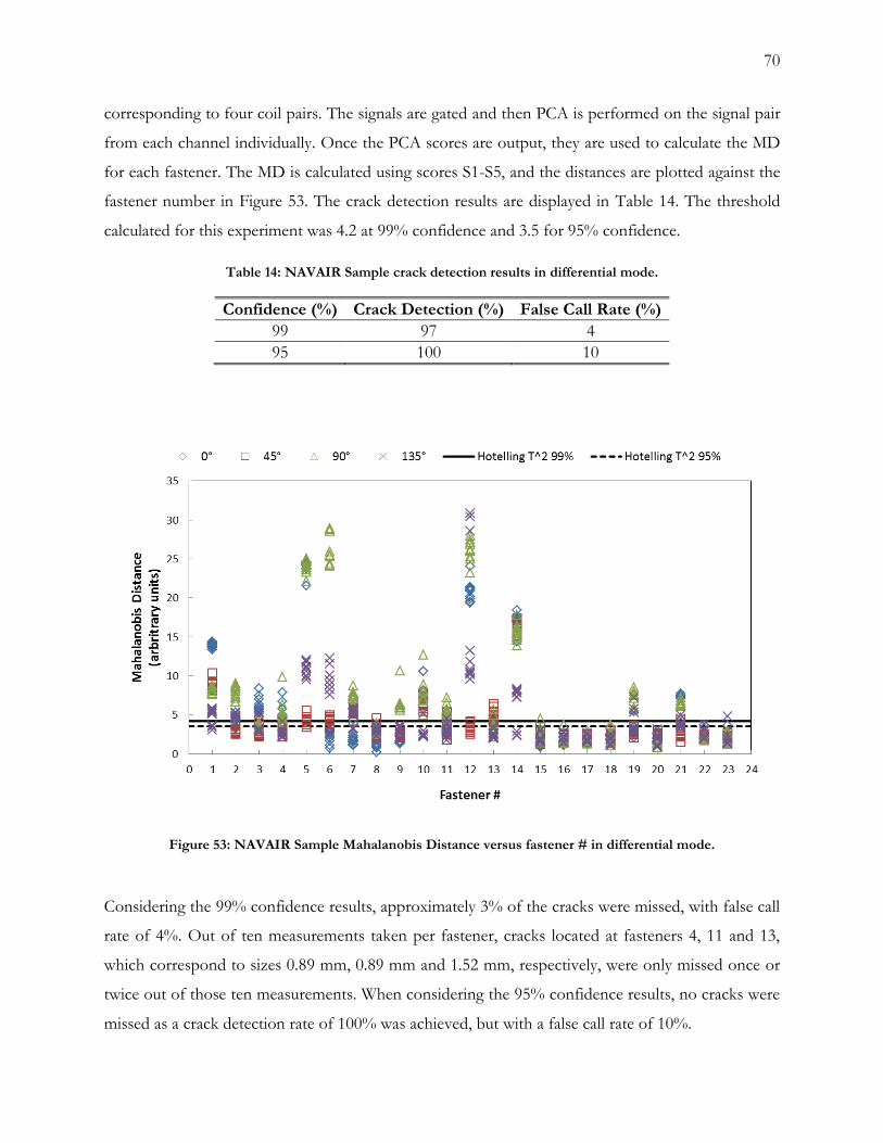
70

corresponding to four coil pairs. The signals are gated and then PCA is performed on the signal pair

from each channel individually. Once the PCA scores are output, they are used to calculate the MD

for each fastener. The MD is calculated using scores S1-S5, and the distances are plotted against the

fastener number in Figure 53. The crack detection results are displayed in Table 14. The threshold

calculated for this experiment was 4.2 at 99% confidence and 3.5 for 95% confidence.

Table 14: NAVAIR Sample crack detection results in differential mode.


99 97 4

95 100 10

Figure 53: NAVAIR Sample Mahalanobis Distance versus fastener # in differential mode.

Considering the 99% confidence results, approximately 3% of the cracks were missed, with false call

rate of 4%. Out of ten measurements taken per fastener, cracks located at fasteners 4, 11 and 13,

which correspond to sizes 0.89 mm, 0.89 mm and 1.52 mm, respectively, were only missed once or

twice out of those ten measurements. When considering the 95% confidence results, no cracks were

missed as a crack detection rate of 100% was achieved, but with a false call rate of 10%.

71

5.8.5 Mahalanobis Distance versus Crack Size

As stated in Section 5.8.3, the MD values appear to be correlated with notch size. Referring to

Figure 53, fasteners with the largest crack size, greater than 5.08 mm (fasteners 5, 12 and 14), tend to

produce the largest distance values. In addition, fasteners with the smallest crack size of 0.89 mm

(fasteners 4 and 11) tend to have smaller distance sizes. To investigate this, the largest Mahalanobis

Distance was plotted with crack size (mm) for each of the 100 measurements (ten measurements on

each of ten second layer cracks) and the results are displayed in Figure 54. A line of best fit was

inserted through the data, showing that the relationship between the distance and crack size is

approximately linear with the R2 value equal to 0.89. Both threshold values (4.2 at 99% confidence

and 3.5 for 95% confidence) are depicted on the graph. It is noted that all the cracks fall above the

95% threshold value. This important observation shows the potential for crack sizing using

Mahalanobis Distance.

Figure 54: Mahalanobis Distance versus crack size for NAVAIR Sample second layer cracks in differential mode.

72

5.9 Results on Test Piece #1


Test Piece #1 was fabricated in the lab using 2024-T3 aluminum sheets joined together by a row of

fasteners. The top sheet thickness was 2 mm and the fastener head diameter was 6.5 mm. The piece

contains twenty-nine fasteners of type HL-19. Ten of the fastener holes do not have notches at their

bore. The notches in the remaining 19 fastener holes are in the top-of-bottom layer, and range in

length from 0.83 – 3.26 mm, with minimum notch size slightly less than the minimum 0.89 mm in

the NAVAIR sample.

5.9.2 Eigenvector Selection

Test piece #1 data, using absolute mode analysis, was analyzed with the same number of

eigenvectors that were used to calculate crack detection results on the NAVAIR sample (vectors 1-

5). In order to ensure maximum crack detection results, alternate combinations of scores were

investigated. It was determined on this test piece, in absolute mode, that using eigenvectors three,

four and five to calculate the MD instead of eigenvectors 1-5 yielded better crack detection. Figure

55 shows the first five eigenvectors of absolute mode PCA data on Test Piece #1 from the third coil

pair. The third and fourth eigenvectors have the biggest contribution in the desired timeframe where

eddy current density is greatest (0.4 - 1.0 ms, see Section 3.8.1).

Figure 55: First five eigenvectors of PCA on data from Test Piece #1 third coil pair (concatenated signals) in absolute mode.

1st coil 2nd coil

73

This is in contrast to the NAVAIR sample shown in Figure 49, where the fourth and fifth vectors

peaked in the desired timeframe. Figure 56 shows the results obtained from logistic regression [17]

to the hit/miss data on second layer cracks obtained when scores 3-5 are used to calculate the MD.

In addition, in Figure 56, scores from 1-5 eigenvectors are used to calculate the MD. A 95%

confidence level was used to calculate the Hotelling T2 value for the hit/miss analysis. From this

figure it can be seen that using a combination of the third, fourth and fifth scores (a50 = 1.04 mm)

rather than five (a50 = 1.45 mm) improved the detectability of the majority of crack sizes by shifting

the whole curve to the left. This is counter-intuitive, as one would assume that more terms would

provide better results. However, if scores without information are added to the MD calculation, the

Hotelling T2 value increases faster than the increase in MD.

Figure 56: Results from logistic regression performed on hit miss data from Test Piece #1 using eigenvectors 3-5 and 1-5. Horizontal axis is on a log scale.

5.9.3 Absolute Mode Crack Detection Results

The experimental process described in Section 3.6.3 was performed on Test Piece #1 using the

probe in absolute mode. After signal gating and PCA, the scores S3-S5 were then used to calculate

the MD for each fastener, as stated in Section 5.9.2. The MD is plotted against fastener number and

is displayed in Figure 57, while the crack detection results are shown in Table 15. The threshold

74

calculated for this experiment was 4.6 at 99% confidence and 3.5 for 95% confidence. As discussed

in Section 5.8.4, the larger crack sizes, greater than 2.8 mm (fasteners 14 and 15), tend to produce

larger MD values. This will be investigated in the next section.

Table 15: Test piece #1 crack detection results in absolute mode.


99 53 0

95 82 0

Figure 57: Test Piece#1 Mahalanobis Distance versus fastener # in absolute mode.

Considering the 99% confidence results, approximately 47% of the cracks were missed. Out of the

two measurements taken per fastener, cracks located at fasteners 23 and 28, which were 0.94 mm

and 0.83 mm, respectively, were missed two out of two times. Three cracks located at fasteners 8, 9

and 22 corresponding to sizes 1.47 mm, 1.43 mm, and 1.24 mm, respectively, were also not detected.

In addition, cracks located at fasteners 2, 6 and 17, which were 1.97 mm, 1.94 mm and 1.92 mm,

respectively, were completely missed. When considering the 95% confidence results, cracks located

at fasteners 8, 22 and 28 were not detected. The larger number of misses is attributed to using the

75

probe in absolute mode. Differential mode, which will be investigated next, was more successful

than absolute mode, as on the NAVAIR sample (see Section 5.8.4).

5.9.4 Differential Mode Crack Detection Results

The experimental process described in Section 3.6.3 was performed on Test Piece #1 using the

probe in differential mode. After signal gating and PCA, the scores were used to calculate the MD

for each fastener using scores S1-S5. The MD is plotted against fastener number and is displayed in

Figure 58. The crack detection results are shown in Table 16. The threshold calculated for this

experiment was 6.2 at 99% confidence and 4.8 for 95% confidence.

Table 16: Test Piece #1 crack detection results in differential mode.


99 82 0

95 92 0

Figure 58: Test Piece#1 Mahalanobis Distance versus fastener # in differential mode.

Considering the 99% confidence results, approximately 18% of the cracks were missed with no false

calls. Out of two measurements taken per fastener, a crack located at fasteners 22, 1.24 mm in

76

length, was not detected. Cracks located at fasteners 28, 3, 8, 17, and 2 corresponding to sizes 0.83

mm, 1.17 mm, 1.46 mm, 1.92 mm, and 1.97 mm, respectively, were missed once out of two

measurements. When considering the 95% confidence results, a crack located at fastener 22 was

missed twice out of two measurements and a crack at fastener 28 was missed once out of two

measurements. No false calls were made in this case either.

5.9.5 Mahalanobis Distance versus Crack Size

As stated in Section 5.8.3 and Section 5.8.4, the MD values appear to be correlated with notch size.

Referring to Figure 58, fasteners with the largest crack size, greater than 2.8 mm (fasteners 14 and

15), tend to produce the largest distance values. In addition, fasteners with the smallest crack size of

0.83 mm (fasteners 18 and 28) tend to have smaller distance sizes. The largest Mahalanobis Distance

was plotted with crack size for each of the 190 measurements (ten each on 19 second layer cracks)

and the results are displayed in Figure 59. A line of best fit was inserted through the data, once again

showing that the relationship between the distance and crack size is approximately linear (R2 value

equals 0.6). Both threshold values (6.2 at 99% confidence and 4.8 for 95% confidence) are depicted

on the graph. It is noted that all the cracks greater than 1.23 mm fall above the 95% threshold value.

Figure 59: Mahalanobis Distance versus crack size for Test Piece #1 in differential mode.

77

5.10 Results on Test Piece CP-140-TT-1B


This test piece, which was provided by ATESS, Trenton, contains 33 fasteners, with notches in 21

of the fastener bore holes located in the bottom-of-top layer and top-of-bottom layer. The notches

range in length from 1.53 – 3.81 mm. The top layer thickness is 2.58 mm, the fastener head diameter

is 7 mm and the fasteners are of type HL-51 (not the same as the NAVAIR sample and Test Piece

#1).

5.10.2 Differential Mode Crack Detection Results

The experimental process described in Section 3.6.3 was performed on the Aurora Test Piece (CP-

140-TT-1B) using the probe in differential mode. Only differential mode is considered here because

previous samples indicated that differential analysis generated better results than absolute mode.

After signal gating and PCA, the scores were used to calculate the MD for each fastener using scores

S1-S5. The MD is plotted against fastener number and is displayed in Figure 60, while the crack

detection results are shown in Table 17. The threshold calculated for this experiment was 4.4 at 99%

confidence and 3.7 for 95% confidence.

Table 17: Test piece CP-140-TT-1B crack detection results in differential mode.


99 86 13

95 90 21

78

Figure 60: CP-140-TT-1B Mahalanobis Distance versus fastener # in differential mode.

Considering the 99% confidence results, approximately 14% of the cracks were missed. Out of four

measurements taken per fastener, three second layer cracks located at fasteners 5, 27 and 29

corresponding to lengths of 2.54 mm, 1.52 mm and 2.03 mm were not detected. When considering

the 95% confidence results, a notch located at fastener 27 (1.52 mm length) was missed twice out of

four measurements and a notch at fastener 29 (2.03 mm length) was missed twice out of four

measurements. The false call rate did increase from 13% to 21%, which is a high rate that is

dependent on the threshold used (Hotelling T2 value).

For these results, the threshold was calculated using n=48 (refer to equation 2.50), the number of

blank fasteners (12) times the number of measurements (4). This is the same calculation used for

previous threshold values. If we decrease the value for ‘n’ for these results to 12 (number of blanks

alone), the threshold values for 99% and 95% confidence are 7.9 and 5.8, respectively. Subsequently,

raising the threshold value lowers the crack detection rates to 64% and 80%, respectively, for 99%

and 95% confidence and the false call rates decrease to zero for both confidence intervals.

79

5.10.3 Mahalanobis Distance versus Crack Size Results

As stated in Section 5.8.3 and Section 5.8.4, the MD values are observed to be correlated with notch

size. As shown in Figure 60, fasteners with the largest first layer crack size, greater than 3.2 mm

(fasteners 6 and 26), tend to produce the largest MD values. In addition, fasteners with the smallest

first layer cracks, smaller than 1.3 mm (fasteners 7, 13 and 28), tend to produce smaller distance

values. Also shown in Figure 60, fasteners with the largest second layer crack size, greater than 3.7

mm (fasteners 10 and 16), tend to produce the largest distance values (for second layer only cracks).

In addition, the fastener with the smallest second layer crack, smaller than 1.6 mm (fastener 27), tend

to produce smaller distance values.

The largest Mahalanobis Distance was plotted with crack size (in millimetres) for four first layer and

four second layer notches and the results are displayed in Figure 61. A line of best fit was inserted

through the data, once again showing that the relationship between MD and crack size is

approximately linear (R2 values equal 0.57 and 0.75 for the first layer best fit line and second layer

best fit line, respectively). Both threshold values (5.1 at 99% confidence and 4.2 for 95% confidence)

are depicted on the graph. First, it is noted that all the first layer cracks fall above the 99% line, and

second layer cracks, greater than 2.5 mm, fall above the 95% threshold value. Second, the first layer

cracks tend to produce a greater distance value for the same crack size, i.e. a 3.8 mm crack in the

first layer produces a distance value on average of 27.1, while a 3.8 mm crack in the second layer

produces a distance value on average of 11.2. This means that there is a possibility of not only sizing

cracks in either the first or second layer, but potentially being able to determine in which layer the

crack resides. Difficulty may arise when a fastener contains both and top and bottom layer cracks at

its bore because it is difficult to discern which crack contributes to the value output of the

Mahalanobis Distance calculation.

80

Figure 61: Mahalanobis Distance versus crack size for test piece CP-140-TT-1B in differential mode.

5.11 Comparison of Test Piece Results (Differential Analysis)

Section 5.10.3 discussed how false call rates and crack detection results can vary by changing the

threshold value. In order to compare the results of each test piece, a comparison of no false calls,

5% and 10% false call rates and crack detection results are shown in Table 18. There is no

confidence interval associated with these results, as an arbitrary threshold value was sought to give

5% false call rates. An 87% crack detection rate was achieved on the NAVAIR sample with no false

calls, a 100% crack detection with no false calls on Test Piece #1 and an 80% crack detection with

no false calls was obtained for the CP-140-TT-1B Aurora sample.

A 100% crack detection accompanied by a 5% false call rate could be achieved for the NAVAIR

sample and Test Piece #1. However, only 82% crack detection on the CP-140-TT-1B Aurora test

piece could be achieved when the false call rate was lowered to 5%. In addition, all second layer

cracks were missed when the false call rate was lowered to 5%. Should a 10% false call rate be

tolerated, the Aurora sample crack detection rate only increases to 85%. If a 100% crack detection

rate was desired on the Aurora sample, it would be accompanied by a 65% false call rate. This

81

analysis shows the importance of threshold values, and how to distinguish acceptable false call rates.

A discussion on the implication of false calls is included in the following section.

Table 18: Crack detection results for no false calls, 5% and 10% false call rate.

False Call Rate (%)

Crack Detection Results (%)

NAVAIR Test Piece #1 CP-140-TT-1B

0 87 100 80

5 100 100 82

10 100 100 85

82

6 Discussion

6.1 PCA and Crack Orientation

One of the benefits of viewing PCA scores in three dimensions is that repetitive measurements tend

to cluster together, demonstrating the repeatability of the technique. A second benefit is that scores

obtained when a crack is present at the borehole cluster separately from scores obtained without a

crack. This allows calculation of the distance between clusters, and detection of cracks as outlined in

Section 5. Viewing the PCA scores before calculation of MD can yield additional crack information.

Figure 62 shows a three dimensional PCA space of principal component scores S2, S3 and S4

obtained from the NAVAIR sample in differential mode. Fasteners 8, 17, 20 and 22 are fasteners

without notches at their bore, and each graph contains two groups of scores from two separate

fasteners with notches at their bore, but the notch locations are 180° from each other. In Figure 62

(a), fastener 5 has a notch at orientation C (reference Figure 62 (c) for notch orientations), while

fastener 3 has a notch at D (180° from C), and the scores separate in the PCA space to either side of

the cluster of blanks. The same effect occurs in Figure 62 (b), where fastener 1 has a notch at

orientation A, and fastener 14 has a notch at orientation F, 180° from A. The scores from these two

fasteners lie on either side of the cluster of blanks. In addition, notch orientations A and C are both

on the side closest to the edge of aluminum (see Figure 62 (c), where the second layer aluminum

edge is located at 90°) and both sets of scores in the PCA space tend to congregate on the same side

relative to the cluster of scores from the no-notch fasteners. The same results occur for notch

orientations D and F. Figure 62 (d) shows fastener 4, which has a notch at orientation B, and

fastener 13, which has a notch at orientation E. These scores separate from one another, but are not

located on either side of the cluster of blanks, as in the other two graphs. This is partly due to edge

effects, where the notch at fastener 4 is pointing in the direction of the edge of aluminum in the

bottom layer.

83

Figure 62: Three dimensional depiction of PCA scores S2, S3 and S4 from NAVAIR differential data. Labels

refer to notch orientation as defined in the inserted figure.

6.2 Absolute versus Differential Analysis

Absolute and differential analysis methods were tested on two of the multi-layer test pieces

(NAVAIR and Test Piece #1). Differential mode was chosen to analyze the Aurora sample because

it yielded better crack detection results on the two previous test pieces. In addition, differential

analysis was more robust and consistent than absolute, as absolute analysis required a different

-1.5-1.0-0.500.5

S2

-0.4-0.200.20.40.6

S3

-0.10

-0.05

0

0.05

S4

532220178

-1.5-1.0-0.50 0.5

S2

-0.4-0.200.20.40.6

S3

-0.10

-0.05

0

0.05

S4

1142220178

-1.5-1.0-0.50 0.5

S2

-0.4-0.200.20.40.6

S3

-0.10

-0.05

0

0.05

S4

4132220178

A

B

E F

C

D

Bottom Edge of Sample

(a) (b)

-1.5 0.5

S2

C

D

No-Notch

-1.5 0.5

S2

A

F

No-Notch

(d)

B

E

No-Notch

S2

(c)

84

combination of scores for the MD calculation, whereas differential analysis utilized scores 1-5 for

each test piece.

6.3 Comparison to FEM

Considering the FEM [32] discussed earlier in Section 1.3.4, displacement effects were detected on

the first PCA score. Similar experiments conducted on the single fastener test piece and NAVAIR

sample showed that the effect of displacing the probe over the fastener was large on the first score,

but also had a very minor effect on the second, third and fifth scores. The FEM showed that the

first and third scores provided clear identification of notches, despite large effects due to

displacement of the probe [32]. Results presented in this work showed the presence of a crack was

most strongly correlated with the third score, with weaker correlation with remaining scores (1, 2, 4

and 5). The FEM results did not require more than three PCA eigenvectors to reproduce signals.

However, FEM did not investigate additional factors such as: lift-off, fastener head height and

distance of fastener from the edge, nor did it simulate coil imbalance effects. Due to the logistic

regression results, presented in Section 5.8.2, showing that five eigenvectors produced better crack

detection results than three (three were used in the FEM), this thesis work shows that PCA can

extract additional information contained in the measured PEC signals. The FEM simulations

demonstrated that PEC has the potential to successfully detect cracks, their depths and orientation

in a dual layered aluminum structure. In addition, there was good agreement between the modeling,

and the experimental results presented in Sections 4 and 5, as the FEM demonstrated the same

sensitivity to notch orientation.

6.4 PCA Score Correlations with Variables

The results presented in Section 5 showed how different variables are correlated with PCA scores. A

summary of these correlations is presented in Table 19, for the multiple fastener test piece results in

differential mode. Fastener head height was an important variable to account for in the laboratory

setting, but was effectively eliminated by re-countersinking the top pieces of Test Pieces #1 and 2. It

is important to note that the correlation with the presence of a notch is not separate from other

variables, such as off-centering, lift-off and distance to the edge. This is due to the large number of

variables affecting the transient coil response and is consistent with the requirement of using five

eigenvectors (and their representative scores) to calculate the MD for crack detection.

85

Table 19: Summary of PCA correlations with different variables.

PCA

Score

Off-Centering

(NAVAIR Sample)

Notch (NAVAIR

Sample)

Fastener Head

Height

(Test Piece #2)

Lift-Off

(Test Piece

#2)

Distance to

Edge

(CP-140-TT-

1B)

S1 Yes Yes Yes Yes No

S2 Yes (Weak) Yes Yes Yes No

S3 Yes (Weak) Yes No No No

S4 No Yes (Weak) No Yes (Weak) Yes

S5 Yes (Weak) Yes (Weak) No Yes (Weak) Yes

6.5 Minimum Detectable Flaw Size

6.5.1 General

The differential mode results from the NAVAIR sample, where the smallest notch size was

0.89 mm, showed that 100% of the notches (top and bottom layer) were detected, at 95%

confidence. On test piece #1, the smallest notch size was 0.82 mm (fastener 18), where the overall

notch detection result was 92% (one crack of size 0.83 mm was missed) for the differential analysis

at 95% confidence.

The CP-140 test piece results were not as favourable as the results on the NAVAIR sample and the

lab fabricated test piece. Ninety percent of the EDM notches were detected at 95% confidence,

where two second layer notches, 1.52 mm and 2.03 mm, were missed. One of the reasons why fewer

second layer cracks were detected in the Aurora test piece is that the first layer aluminum was of

thickness 2.58 mm, thicker by 0.55 mm than the NAVAIR sample and test piece #1. Detection

would be hampered by the requisite penetration depth as described in Equation 2.28, resulting in

poorer crack detection results. In addition, the fasteners were a different type in the Aurora sample

(HL-51) than the fasteners in the NAVAIR sample and test piece #1 (HL-19). A variation in

fastener type will correspond to different material and alloying, and subsequently diverse values of

permeability and conductivity (using conventional eddy current, it was determined that the different

86

fasteners do demonstrate a lower permeability). A change in fastener permeability will affect

magnetization of the fastener, and subsequently the magnitude of the induced eddy currents [25].

NAVAIR and Test Piece #1 are very comparable at 5% false call rate, as shown in Table 18 in

Section 5.11. Test Piece #1, with 100% detection at 0% false call rate compared with the NAVAIR

sample’s 87% detection at 0% false call rate, yielded slightly better results. This can be attributed to a

smaller diameter fastener, which relative to the ferrite core diameter, improves detection [2].

A goal is to determine the minimum flaw size that is detectable using PEC. For comparison, in

conventional techniques, where fastener removal is employed, the targeted minimum detectable flaw

size for second layer cracks in a multi-layer aluminum lap joint is 0.76 mm (0.030 inches). Using this

PEC technique, fastener removal is not required, eliminating the risk of collateral damage to the

surface and bore hole caused during fastener removal.

6.5.2 First Layer Notches

The smallest first layer notch (bottom-of-top layer) out of the three multi-layer samples (NAVAIR

sample, Test Piece #1 and Aurora sample) was 1.27 mm. If we consider that the minimum reliably

detectable flaw size using the conventional eddy current technique 140-306-E [6] for first and

second layer cracks is 2.54 mm, then results using the PEC probe in differential mode exceed this

detectability. All first layer notches (1.27 mm and larger) were detected, at 95% confidence.

Therefore, this PEC technique shows potential to improve the minimum detectable flaw size for

first layer cracks to 1.27 mm, without removing fasteners.

6.5.3 Second Layer Notch Detection

The smallest second layer notch out of all three multiple-layer test pieces was 0.82 mm. The

Canadian Armed Forces eddy current surface inspection technique [6] for first and second layer

defects in CP-140 Aurora lap joint fastener holes can reliably detect first and second layer notches

2.54 mm in length. However, it has limitations in detecting defects in the 0°, 90°, 180° and 270°

defect locations, and also requires probe rotation. Test results from the three multi-layer test pieces

show that this PEC technique has surpassed the minimum detectable flaw size of 2.54 mm

achievable using technique 140-306-E, and that the technique is approaching the BHEC minimum

detectable flaw size (defined in Section 1.1) of 0.76 mm, where fastener removal is required. This is

comparable to the results obtained here for the NAVAIR and Test Piece #1 samples, where

87

minimum flaw sizes of 0.89 mm and 0.83 mm, respectively, could be detected with 5% false call rate.

Further work is required to establish a minimum detectable flaw size (a90/95) for PEC technique.

6.6 False Call Rates

The probability of false calls was defined in Section 2.11, and false call rates were calculated for each

set of results on each test piece, depending on confidence level (either 99% or 95%). Considering

the 95% confidence interval results for the NAVAIR sample and Test Piece #1 differential data,

false call rates were 10% and 0%, respectively. On the Aurora test piece, the differential mode test

results yielded a 21% false call rate.

The costs associated with false calls are important for understanding the effectiveness of a

technique. Using a 95% confidence interval, a 5% false call rate could be expected; however, two of

the test pieces had false call rates above 5%. A larger sample set, including a significant number of

blanks, would help improve the statistics of this comparison. If a crack is detected, above the critical

crack size, the operator could flag the fastener location, remove the fastener, and perform a BHEC

inspection [7], which is capable of reliably detecting 0.76 mm flaws.

6.7 Sources of Uncertainty

6.7.1 Coil Balancing

Coil-based probes are used for conventional eddy current testing and are also being utilized for

research in pulsed eddy current techniques. Coil-based probes with two or more coils require careful

construction for coil pair matching, to ensure that each coil pair responds in a similar manner. Each

individual coil was sensitive to placement in the probe, i.e. the signal amplitude varied with distance

from probe face. Achieving exact coil balance for eight coils (four coil pairs) was difficult to achieve.

Coil imbalance explains why some coil pairs were more sensitive to the presence of cracks than

others.

88

7 Conclusions and Recommendations

7.1 Conclusions

The motivation for this thesis work was detection of second layer cracks in aluminum lap joints,

without ferrous fastener removal, thereby reducing inspection times and potential damage to aircraft.

A pulsed eddy current technique was developed, which is capable of detecting cyclic fatigue cracks

emanating from around fastener holes in variable directions, with fasteners present. The capability of

the technique was shown to approach that of conventional BHEC, and has the added benefit of not

requiring fastener removal.

A probe design, consisting of a driving coil wound on a ferrite core with symmetrically located pick-

up coils placed over the fastener, is utilized. The probe takes advantage of magnetization by the

driving coil of the ferrous fastener, which then acts as a pathway for flux, allowing for deeper

penetration of the eddy currents into the surrounding aluminum structure. The probe design has

eight pick-up coils, which were used to detect notches emanating in multiple directions from around

the fasteners.

A method to distinguish subtle differences between signals from fasteners with and without cracks

at their bore was employed due to the similarity between signals from the crack and no-crack case.

This statistical technique, called Principal Components Analysis, reduced signals to scores and

vectors that describe the maximum amount of variation between them. The relative distance, or

Mahalanobis Distance, of a cluster of PCA scores in the presence of a notch to the cluster of PCA

scores from blanks was calculated. The distance values were compared to a threshold value,

calculated using Hotelling T2 theory and based on 99% and 95% confidence intervals.

Experiments conducted on three multiple fastener test pieces of similar construction show that

notches ranging in size from 0.8-5.5 mm were detectable using the coil-based probe centered over

ferrous fasteners. The three samples consisted of 2024-T3 aluminum, but contained different

fastener types and sizes. Optimum results were obtained using analysis of differential signals from

opposing paired coils, and PCA scores 1-5 at 95% confidence interval. The NAVAIR sample

contained HL-19 fasteners with head diameter of 7 mm and first layer thickness of 2 mm. EDM

notches, ranging in size from 0.89 mm to 5.46 mm, were present in the first and second layers.

Crack detection of 100% was achieved, with 5% false calls. Test piece #1 was lab fabricated,

89

contained HL-19 fasteners with head diameter of 6.5 mm and had a first layer thickness of 2 mm.

Notches ranging in size from 0.82 mm to 3.26 mm were present in the second layer. Test piece #1

yielded 100% crack detection, with 5% false calls. The CP-140 Aurora piece contained HL-51

fasteners with head diameter of 7 mm, and first layer thickness of 2.58 mm. This test piece yielded

82% crack detection with 5% false calls.

Mahalanobis Distance was shown to be correlated with crack size. Smaller cracks tended to produce

smaller MD values, whereas larger cracks produced much larger MD values. In addition, first layer

cracks produced MD values larger than second layer cracks, for the same crack size. This result

identifies a potential means for sizing cracks and identifying in which layer they reside.

Out of all the test pieces, all first layer notches were detected, showing a major improvement over

the current method of first layer crack detection with fasteners installed [6], which can only reliably

detect flaws of length 2.54 mm and greater. PEC second layer notch detection surpasses the

minimum detectable flaw size provided using conventional EC technique 140-306-E [6], and

approaches the minimum detectable flaw size for BHEC. Should a flaw be detected, a BHEC

inspection [7] could be performed, after fastener removal, to confirm the presence of a crack.

These results provide strong evidence that pulsed eddy current has the capability for second layer

crack detection in multi-layer aluminum structures, such as lap joints, approaching the target crack

size of 0.76 mm (the minimum detectable flaw size using BHEC [9]). Principal components analysis

has been demonstrated as a viable method of reducing signals to fewer dimensions, making

subsequent discrimination between scores from fasteners with notches present and fasteners

without, easier. PCA also provides a mechanism for compensating for additional variables that may

affect PEC signal response (lift-off, fastener head height and variable distance from edge).

Introducing Mahalanobis Distance analysis of the PCA scores provided a reliable and consistent way

of further discriminating between the two groups of scores, and also shows promise for crack sizing.

7.2 Recommendations

The Mahalanobis Distance analysis is dependent on known samples; in other words, knowing which

fasteners do not contain notches at their bore. This is because the covariance matrix is made up of

PCA scores from blanks, which is then applied to the other fasteners to calculate their MD values.

In order to apply this method to an unknown set of measurements, it would be more expeditious to

search for “outliers” or PCA scores that do not belong with the PCA scores from blanks, based only

90

on their position in the PCA space (not requiring calibration). It is suggested that the fast algorithm

for the minimum covariance determinant estimator [41], which generates an initial estimate of the

covariance matrix and uses a selective iterative process to determine the minimum covariance

matrix, be used. This process would seek to identify outliers in the data (in our case, an outlier would

be a PCA score belonging to a fastener with a crack present). This work requires large data sets, and

the assumption that the majority of data points are from fasteners that do not contain cracks at their

bore, which is normally the case for typical aircraft structure inspections.

The test pieces used for this thesis work all contain notches, which were either electrically discharge

machined (EDM) or cut with a band saw blade. In order to determine if this process will reliably

detect cyclic fatigue cracking from around ferrous fasteners in the second layer, testing should be

conducted on actual fatigue cracks, grown in a lab setting, ideally on test pieces taken from service.

Occasionally, fasteners are replaced during maintenance procedures by different types. These

fasteners can be made of different ferrous materials, titanium or even aluminum. It is beneficial to

conduct measurements using different fastener materials in order to understand the PEC system

response, and subsequently the crack detection ability.

Results from this work showed clusters of PCA scores from one crack orientation separated from

clusters from other crack orientations, with respect to blanks. It is recommended that crack

propagation directions be analyzed using vector analysis, potentially in spherical coordinates, where

the MD value represents the distance from the origin (center of the blank cluster) and angles are

measured in polar and azimuthal coordinates [10].

Giant Magnetoresistive Sensors (GMRs) have been used in previous studies, specifically for

detecting SCC around ferrous fasteners in the inner wing spar of CF-188 aircraft [26]. GMRs detect

the magnetic field directly, and were successful in detecting SCC in the aforementioned work. Yang

et al. [42] designed a system using a multiline coil to generate the magnetic field, and GMRs to sense

the transient field. Using time and frequency domain features, they successfully detected small cracks

under fasteners at depths up to 10 mm. It would be relevant to construct a probe using the same

driving coil ferrite core combination, but with GMRs as the sensing element to determine if the

same level or improved crack detection is possible.

91

Surface and internal damage caused by fastener removal/re-installation can cause noise in the

acquired signals that may cause false calls to arise. An investigation into the sensitivity of this PEC

system to surface and fastener hole damage is suggested to ensure accurate and reliable results.

When an optimized probe design is achieved, whether by using coils or GMRs, a hit/miss or a-hat

versus a probability of detection (POD) study should be carried out to determine the a90/95, i.e. the

crack size above which 90% of the cracks are detected 95% of the time. This study requires a

minimum number of flawed and unflawed sites, as well as a proper crack size distribution around

the target size to be detected. In addition, the first layer thickness should be varied in order to assess

the ability of PEC to detect second layer cracks at a variety of first layer depths.

This technique could potentially be applied to other applications where second layer cracking occurs.

This does not have to be specific to wing skin applications, but could possibly extend to any area of

the aircraft where either backside access is prohibited, and the first layer is not too thick so as to

allow for good penetration and detection of transient eddy current induced fields.

92

References

[1] D. E. Bray and R. K. Stanley, Nondestructive Evaluation, A Tool for Design, Manufacturing

and Service, United States of America: McGraw Hill Inc, 1989.

[2] P. P. Whalen, "Transient Eddy Current Inspection in the Presence of Ferrous Fasteners in

Multi-Layered Aluminum Structures, Master Applied Science Thesis," RMC, Kingston, 2010.

[3] Materials Handbook, Non-Destructive Evaluation and Quality Control, Ninth ed., vol. 17,

Metals Park, Ohio: ASM International, 1098.

[4] A. Sophian, G. Y. Tian, D. Taylor and J. Rudlin, "Design of a pulsed eddy current sensor for

detection of defects in aircraft lap joints," Sensors and Actuators, vol. 101, pp. 92-98, 2002.

[5] N. E. Dowling, Mechanical Behaviour of Materials, 4th ed., New Jersey: Pearson Education

Inc., 2013.

[6] Canadian Forces Eddy Current Inspection, "Technique # 140-306-E, CP-140 Wing Planks Lap

Joint Fastener Holes," 2007.

[7] Canadian Forces Eddy Current Inspection, "General Bolt Hole Technique for Metallic

Structures," 2008.

[8] Depertment of Defense, Nondestructive Evaluation System Reliability Assessment, MIL

HDBK 1823A, Department of Defense, 2009.

[9] R. Short, CP140 minimum Inspectable Flaw Sizes for DTA Following Select NDI, 2012.

[10] J. D. Griffiths, Introduction to Electrodynamics, Upper Saddle River: Prentice-Hall, 1999.

[11] V. S. Cecco, G. Van Drunen and F. L. Sharp, Manual on Eddy Current Method, vol. 1, Chalk

River, ON: Chalk River Nuclear Laboratories, 1981.

[12] R. A. Smith and G. R. Hugo, "Deep corrosion and crack detection in aging aircraft using

93

transient eddy current NDE," in 5th Joint NASA/FAA/DoD Aging Aircraft Conference, 2001.

[13] T. W. Krause, C. Mandache and J. H. Lefebvre, "Diffusion of Pulsed Eddy Currents in Thin

Conducting Plates," vol. 975, 2008, pp. 368-375.

[14] I. Z. Abidin, C. Mandache, G. Y. Tian and M. Morozov, "Pulsed eddy current testing with

variable duty cycle on rivet joints," NDT&E International, vol. 42, no. 7, pp. 599-605, 2009.

[15] T. J. Cadeau, "Increased Field Depth Penetration with Pulsed Eddy Current," RMC, Kingston,

2008.

[16] P. Horan, P. Underhill and T. W. Krause, "Pulsed eddy current detection of cracks in F/A-18

inner wing spar without wing skin removal using modified principal components analysis,"

NDT&E International, vol. 55, pp. 21-27, 2013.

[17] J. Lattin, J. D. Carroll and P. E. Green, Analyzing Multivariate Data, Pacific Grove:

Brooks/Cole, 2003, pp. 4, 264-275.

[18] Y. He, F. Luo, M. Pan, F. Weng, X. Hu, J. Gao and B. Liu, "Pulsed eddy current technique for

defect detection in aircraft riveted structures," NDT&E International, vol. 43, pp. 176-181, 2009.

[19] V. B. Wwdensky, "Concerning the eddy currents generated by a spontaneous change of

magnetization," Annalen de Physik, vol. 64, pp. 609-620, 1921.

[20] J. D. Jackson, Classical Electrodynamics, California: John Wiley & Sons, INC, 1999.

[21] C. V. Dodd and W. E. Deeds, "Analytical solutions to eddy current coil probe problems,"

Journal of Applied Physics, vol. 39, no. 6, pp. 2829-2838, 1968.

[22] D. P. Desjardins, T. W. Krause, A. Tetervak and L. Clapham, "Concerning the derivation of

exact solutions to inductive circuit problems for eddy current testing," NDT&E International,

no. Submitted, 2014.

[23] D. R. Desjardins, G. Vallieres, P. P. Whalen and T. W. Krause, "Advances in Transient (Pulsed)

Eddy Current For Inspection of Multi-Layer Aluminum Structures in the Presence of Ferrous

94

Fasteners," Review of Progress in Quantitative Nondestructive Evaluation, pp. 400-407, 2012.

[24] M. N. Sadiku, Elements of Electromagnetics, Third ed., New York: Oxford University Press,

2001.

[25] V. K. Babbar, P. P. Whalen and T. W. Krause, "Pulsed Eddy Current Probe Development to

Detect Inner Layer Cracks near Ferrous Fasteners Using COMSOL Modeling Software," in

COMSOL Conference, Boston, 2012.

[26] P. F. Horan, Pulsed eddy current inspection of CF-188 inner wing spar, Master's Applied

Science Thesis, Kingston: RMC, 2013.

[27] P. F. Horan, P. R. Underhill and T. W. Krause, "Real Time Pulsed Eddy Current Detection of

Cracks in F/A-18 Inner Wing Spar Using Discriminant Separation of Modified Principal

Components Analysis Scores," IEEE Sensors, vol. 14, no. 1, pp. 171-177, 2014.

[28] S. Giguere, B. A. Lepine and J. M. Dubois, "Pulsed Eddy Current Technology: Characertizing

Material Loss with Gap and Lift-off Variations," Research in Non-destructive Evaluation, vol. 13, pp.

119-129, 2001.

[29] K. I. Kim, K. Jung and H. J. Kim, "Face recognition using kernel principal components

analysis," IEEE Signal Processing Letters, vol. 9, no. 2, pp. 40-42, 2002.

[30] J. Yu, "Fault detection using principal components-based gaussian mixture model for

semiconductor manufacturing processes," IEEE Transactions on Semiconductor Manufacturing, vol.

24, no. 3, pp. 432-444, 2011.

[31] P. R. Underhill, A. Tetervak and T. W. Krause, "PEC Detection of Cracks in Aluminum

Structures in the Presence of Ferrous Fasteners using Modified Principal Component Analysis,"

in Smart Materials and CINDE Conference, Montreal, Nov 2-4 2011.

[32] V. K. Babbar, P. R. Underhill, C. Stott and T. W. Krause, "Finite Element Modeling of Second

Layer Crack Detection in Aircraft Bolt Holes with Ferrous Fasteners Present," NDT&E

International, vol. 65, pp. 64-71, 2014.

95

[33] G. Niu, S. Sinch, S. W. Holland and M. Pechy, "Health monitoring of electronic products based

on Mahalanobis Distance and Weibull decision metrics," Microelectrics Reliability, vol. 51, pp. 279-

284, 2011.

[34] G. Cosarinsky, M. Ruch, G. Rugirello and G. Domizzi, "Eddy Current Testing Reliability

Improvement; Application to Nuclear Fuel Cladding Tubes," in VIII Con greso Regional de

ENDE, 2011.

[35] R. De Maesschalck, D. Jouan-Rimbaud and D. L. Massart, "Tutorial: The Mahalanobis

Distance," Chemometrics and Intelligent Laboratory Systems, pp. 1-18, 2000.

[36] "NDT Resource Center," 2001. [Online]. Available: http://www.ndt-

ed.org/GeneralResources/Formula/ECFormula/Cond-Resist/CondResist.htm. [Accessed 25

11 2012].

[37] H. C. Ohanian, "On the approach to electro- and magneto-static equilibrium," in American

Association of Physics Teachers, 1983, pp. 1020-1022.

[38] S. Goldman, Transformation Calculus and Electrical Transients, New York: Prentice Hall Inc.,

1949, pp. 90-92.

[39] A. Sophian, G. Y. Tian, D. Taylor and J. Rudlin, "A feature extraction technique based in

pricipal component analysis for pulsed eddy current NDT," NDT&E International, vol. 36, pp.

37-41, 2003.

[40] "e-Handbook of Statistical Methods," NIST/SEMATECH , [Online]. Available:

http://www.itl.nist.gov/div898/handbook/eda/section3/eda3665.htm. [Accessed 9 January

2014].

[41] P. J. Rousseeuw and K. V. Driessen, "A Fast Algorithm for the Minimum Covariance

Determinant Estimtor," Technometrics, vol. 41, no. 3, pp. 212-223, 1999.

[42] G. Yang, A. Tamburrino and L. Upda, "Pulsed Eddy Current Based Giant Magnetoresistive

System for the Inspection of Aircraft Structures," IEEE, vol. 46, no. 3, 2010.

96

97

Annex A

HL-19-5-5 Technical Information

98

Annex B

HL-51 Technical Information

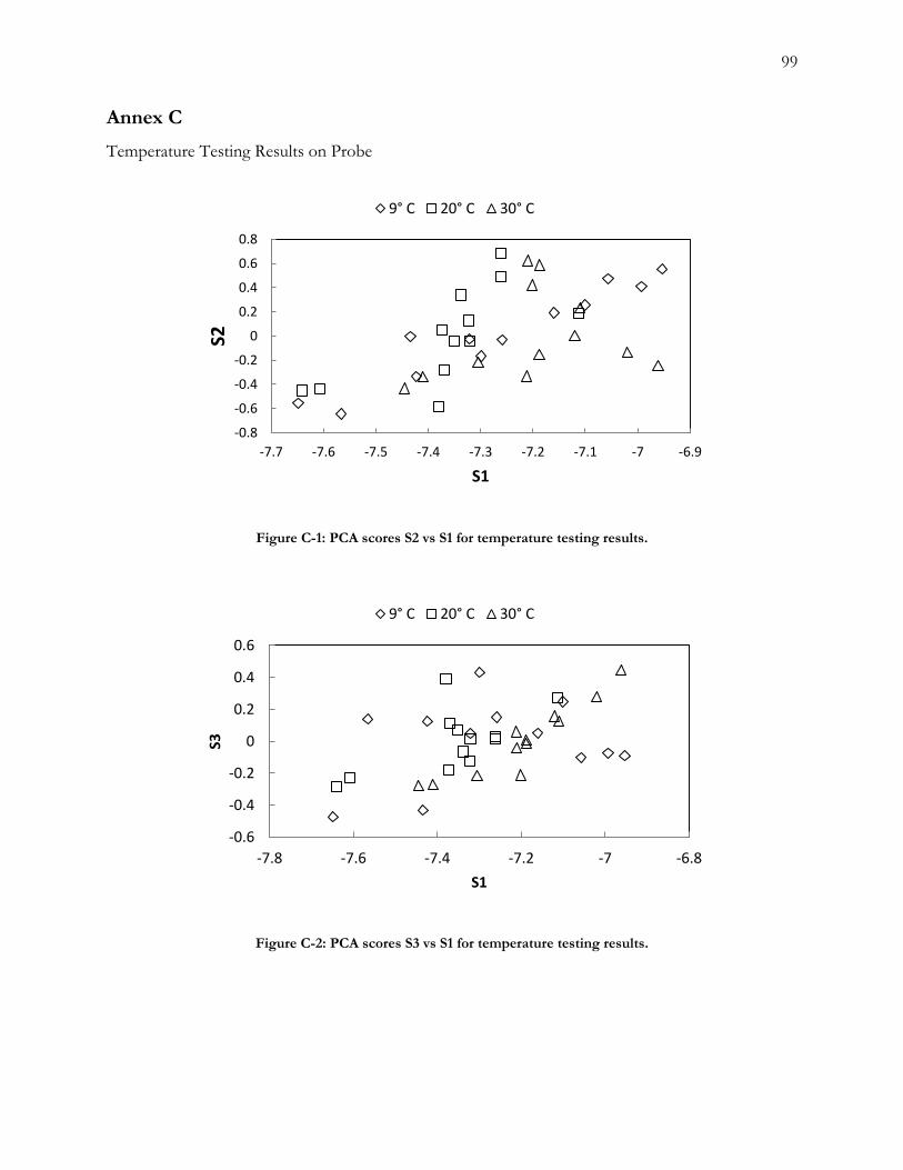
99

Annex C

Temperature Testing Results on Probe

Figure C-1: PCA scores S2 vs S1 for temperature testing results.


-0.8

-0.6

-0.4

-0.2

0

0.2

0.4

0.6

0.8

-7.7 -7.6 -7.5 -7.4 -7.3 -7.2 -7.1 -7 -6.9

S2

S1

9° C 20° C 30° C

-0.6

-0.4

-0.2

0

0.2

0.4

0.6

-7.8 -7.6 -7.4 -7.2 -7 -6.8

S3

S1

9° C 20° C 30° C

100


-0.6

-0.4

-0.2

0

0.2

0.4

0.6

-0.8 -0.6 -0.4 -0.2 0 0.2 0.4 0.6 0.8

S3

S2

9° C 20° C 30° C

101

Curriculum Vitae

102

Curriculum Vitae

Captain Colette Stott, neé Gardiner, was born in Glace Bay Nova Scotia on 24 September 1985. She

obtained a Bachelors of Mechanical Engineering Degree from the Department of Mechanical

Engineering at the Royal Military College of Canada in May 2008. Upon graduation, she attended

Aerospace Engineering Officer Basic Training in Borden Ontario, and was subsequently posted to

427 Special Operations Aviation Squadron in Petawawa Ontario. She served as the Maintenance

Support Officer, and the Deputy Squadron Aircraft Maintenance Engineering Officer, as well as the

Aircraft Fluids Safety Officer until 2012.

Upon completing her tour in Petawawa, Colette was posted to Kingston Ontario to complete a

Masters of Applied Science in Chemistry and Chemical Engineering at the Royal Military College of

Canada.

Papers published in referred, peer reviewed, scholarly journals:

V. K. Babbar, P. R. Underhill, C. Stott and T. W. Krause, "Finite Element Modeling of Second

Layer Crack Detection in Aircraft Bolt Holes with Ferrous Fasteners Present," NDT&E

International, vol. 65, pp. 64-71, 2014.

Submitted Papers:

C.A. Stott, P.R. Underhill, T.W. Krause, ‘Pulsed Eddy Current Detection of Cracks in Multilayer

Aluminum Lap Joints’, IEEE Sensors Journal, submitted June 2014.

Invited Talks and Papers Presented at Major Conferences and Symposia:

C.A. Stott, P.R. Underhill and T.W. Krause, ‘Pulsed Eddy Current Detection of Second Layer

Cracks in Aluminum Aircraft Lap Joints using Cluster Analysis’, Invited Talk to the Department of

Physics Colloquium, Royal Military College of Canada, Kingston, ON, 10 April, 2014.

C.A. Stott, P.R. Underhill and T.W. Krause, ‘Detection of second layer fatigue cracks around ferrous

fasteners in lap joints of a CP-140 Aurora’, NDT in Canada Conference, Toronto, ON, 16-18 June,

2014.

Documents

PULSED EDDY CURRENT INSPECTION OF …. Stott MASc Thesis... · Signed by the final examining committee: / Signé par les membres du comité examinateur de la soutenance de thèse