Embed Size (px)
Citation preview
Progress in the radiative modeling of ice
clouds and dust aerosols for MODIS-based
remote sensing
Ping Yang1,2 and George Kattawar2!
! ! ! ! 1. Department of Atmospheric Sciences!
! ! ! ! 2. Department of Physics &Astronomy!
Texas A&M University, College Station, TX 77843!
In collaboration with !
Andrew Dessler, Gerald North!
Bryan Baum, Andrew Heymsfield, Yongxiang Hu!
Steven Platnick, Michael King, Bo-Cai Gao, Zhibo Zhang!
Si-Chee Tsay, Christina N. Hsu, Istvan Laszlo and Ralph Kahn!
with contributions by
L. Bi, H.-M. Cho, S. Ding, Q. Feng, G. Hong, Y .Li, K. Meyer, Y. Xie, Y. You

The MODIS cloud property products provide an
unprecedented opportunity to
•! develop the climatologies of cloud microphysical
and optical properties from a global perspective
•! assess the performance of climate models
- Data: GSFC-MODIS and LaRC-MODIS Aqua
level 3 (1º!1º) daytime only cloud property products
- Range: July 2002 to June 2007, 60ºN to 60ºS
-CAM3: T42 (128 by 64), 26 vertical levels
- Use observed monthly mean sea surface
temperature and sea ice concentration (Hurrell et al.,
2008) to force the climate model

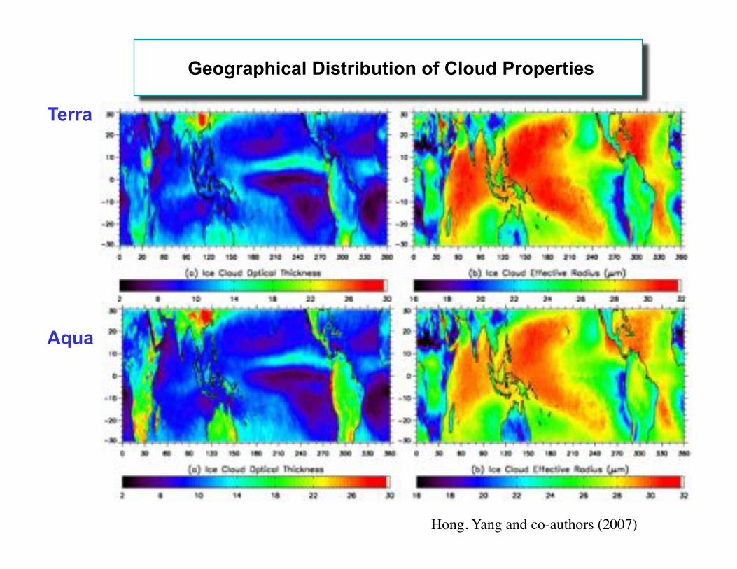
Terra Aqua
Hong, Yang and co-authors (2007)
Geographical Distribution of Cloud Fraction
Terra
Aqua
Geographical Distribution of Cloud Properties
Hong, Yang and co-authors (2007)
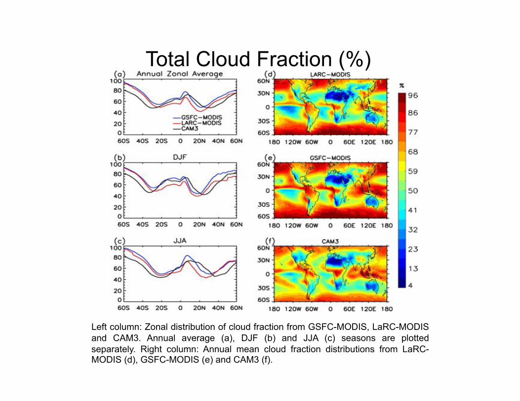
Total Cloud Fraction (%)
Left column: Zonal distribution of cloud fraction from GSFC-MODIS, LaRC-MODIS
and CAM3. Annual average (a), DJF (b) and JJA (c) seasons are plotted
separately. Right column: Annual mean cloud fraction distributions from LaRC-MODIS (d), GSFC-MODIS (e) and CAM3 (f).

Cloud Liquid Water Path ( ) 2
gm!
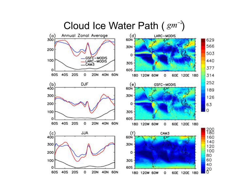
Cloud Ice Water Path ( ) 2
gm!
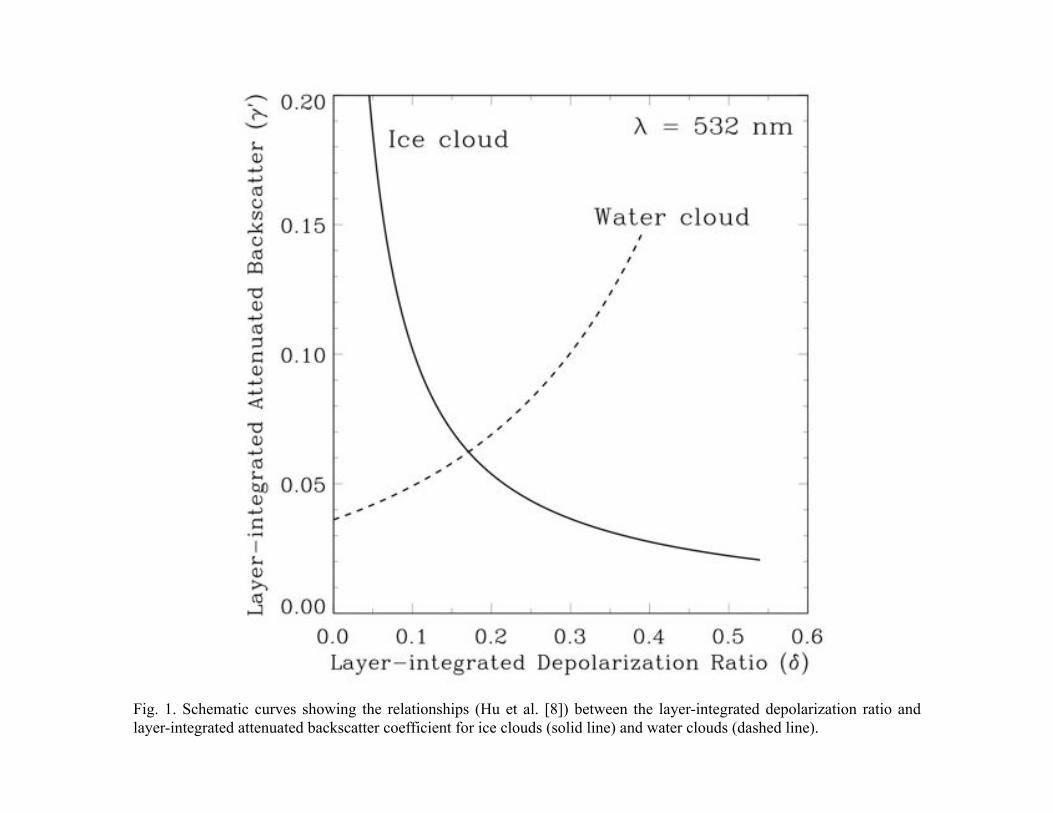
Fig. 1. Schematic curves showing the relationships (Hu et al. [8]) between the layer-integrated depolarization ratio and
layer-integrated attenuated backscatter coefficient for ice clouds (solid line) and water clouds (dashed line).

The
!
" # $ % relationships for the clouds flagged as in water-phase by the MODIS IR cloud-
phase determination algorithm .
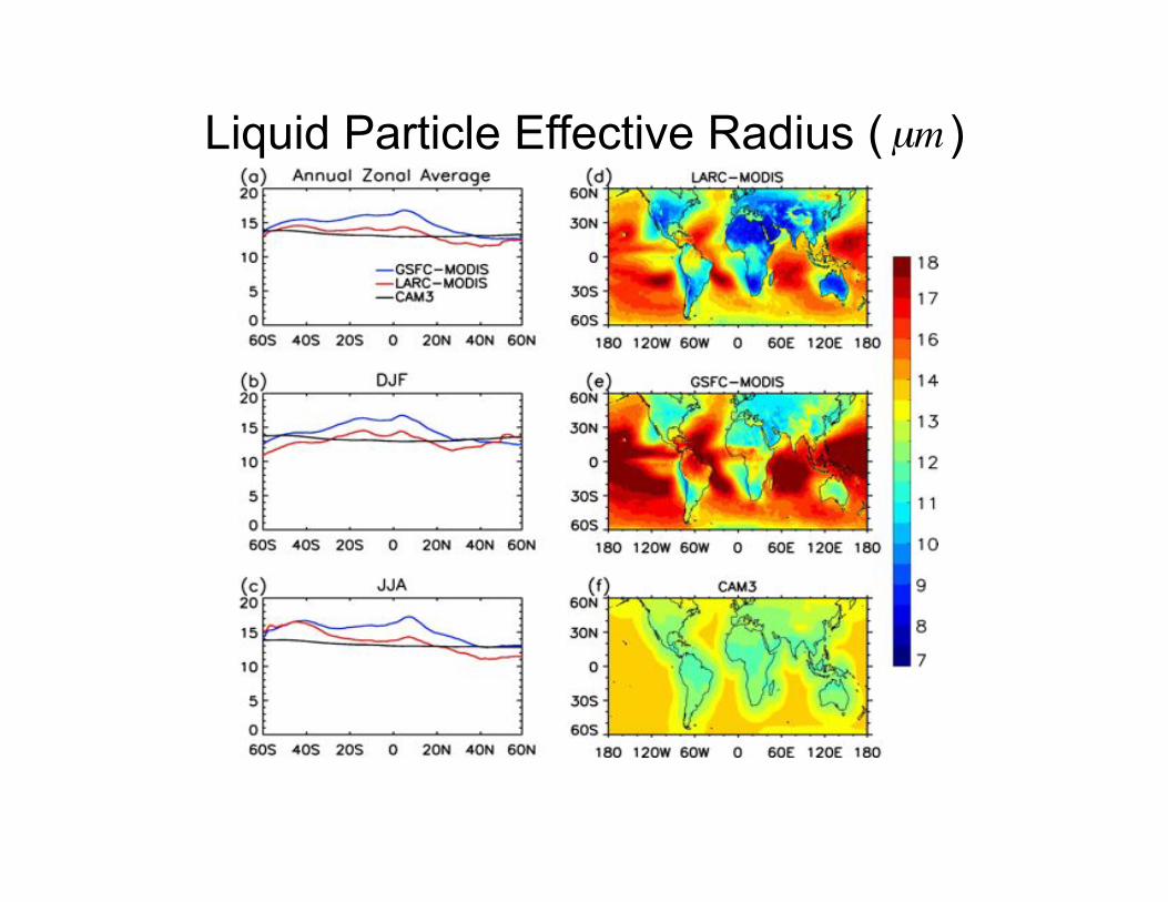
Liquid Particle Effective Radius ( )
!
µm
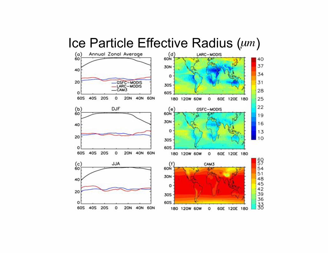
Ice Particle Effective Radius ( )
!
µm
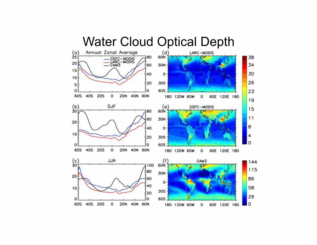
Water Cloud Optical Depth

Ice Cloud Optical Depth

Equatorial Wave Spectrum
Wheeler and Kiladis,1999


!"#$%&'"()$*+,-.(("/$01&2/&-$+3$/&4$566$&,"/&2"7$
8"94""'$:;°<$&'7$:;°=$+3$>"&/$?@@;$3/+-$AB0C=$DEF&$
7&9&G$6H"$9H1IJ$(1'"$I+//"K%+'7K$9+$%H&K"$K%""7$+3$:;$
-KL:$
M12H9$%&'"()$!+'219F7"L(&27&>$I/+KK$K"IN+'$+3$OOBP$;$
+3$566$&,"/&2"7$8"94""'$;°<$&'7$;°=G$Q'19K$&/"$
&/819/&/>G$
6H"$9H1IJ$(1'"$1'71I&9"K$&$%H&K"$K%""7$+3$R$$-KL:$
Light scattering and radiative transfer
simulations are fundamental to the
retrieval of cloud and aerosol
properties from MODIS
measurements
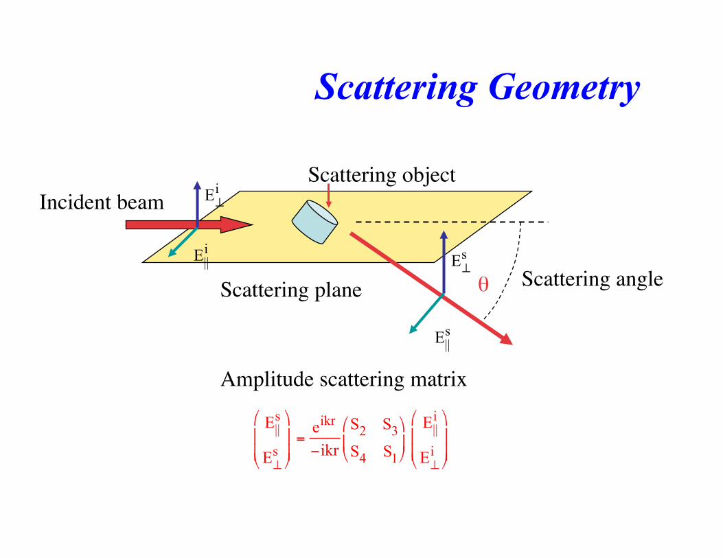
Scattering plane!
Scattering Geometry
Scattering angle!!!
E||
s
E!s
Scattering object!
Amplitude scattering matrix!
E||s
E!s
"
#
$$
%
&
''=
eikr
(ikr
S2 S3
S4 S1
"
#$
%
&'
E||i
E!i
"
#
$$
%
&
''
Incident beam! E!i
E||
i

Stokes vector-Phase matrix/Mueller
matrix formulation
The electric field can be resolved into components. E// and E" are complex oscillatory functions.
!
E = E// l + E" r!
The four component Stokes vector (Stokes, 1852) can now be defined, which are all real numbers.!
I= E// E//* + E" E"
*!
Q= E// E//* - E" E"
*!
U= E// E"*+ E" E//
* !
V= i(E// E"*- E" E//
*)!
Ellipticity= Ratio of semiminor to semimajor axis of polarization ellipse=b/a!
=tan[(sin-1(V/I))/2]!

Nissan car viewed in mid-wave infrared!
!!!!!This data was collected using an Amber MWIR InSb imaging array
256x256. The polarization optics consisted of a rotating quarter wave plate and a
linear polarizer. Images were taken at eight different positions of the quarter wave
plate (22.5 degree increments) over 180 degrees. The data was reduced to the full
Stokes vector using a Fourier transform data reduction technique. Courtesy of
Brume Blume, Nicoholls Co. !
I! Ellipticity!
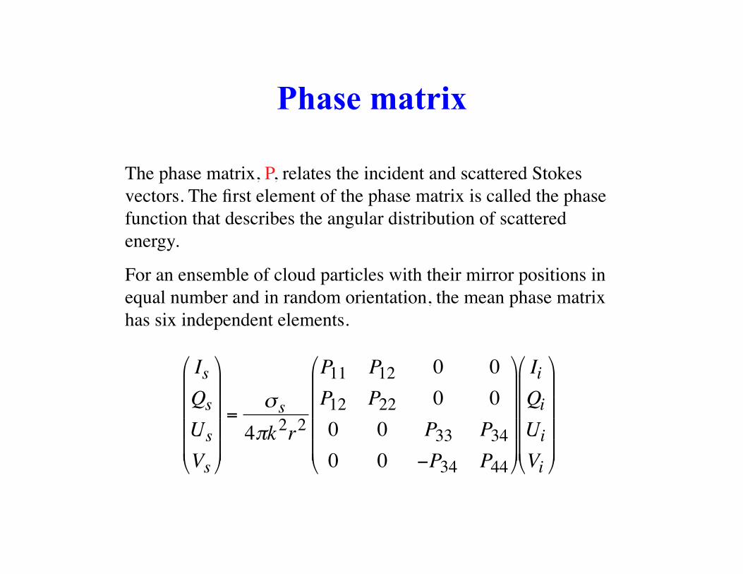
Phase matrix
The phase matrix, P, relates the incident and scattered Stokes
vectors. The first element of the phase matrix is called the phase
function that describes the angular distribution of scattered
energy.!
For an ensemble of cloud particles with their mirror positions in
equal number and in random orientation, the mean phase matrix
has six independent elements. !
!
Is
Qs
Us
Vs
"
#
$ $ $ $
%
&
' ' ' '
=( s
4)k2r2
P11 P12 0 0
P12 P22 0 0
0 0 P33 P34
0 0 *P34 P44
"
#
$ $ $ $
%
&
' ' ' '
Ii
Qi
Ui
Vi
"
#
$ $ $ $
%
&
' ' ' '

Yang, P. and K. N. Liou, 2006: Light Scattering and Absorption by Nonspherical Ice Crystals,
in Light Scattering Reviews: Single and Multiple Light Scattering, Ed. A. Kokhanovsky,
Springer-Praxis Publishing, Chichester, UK, 31-71. !
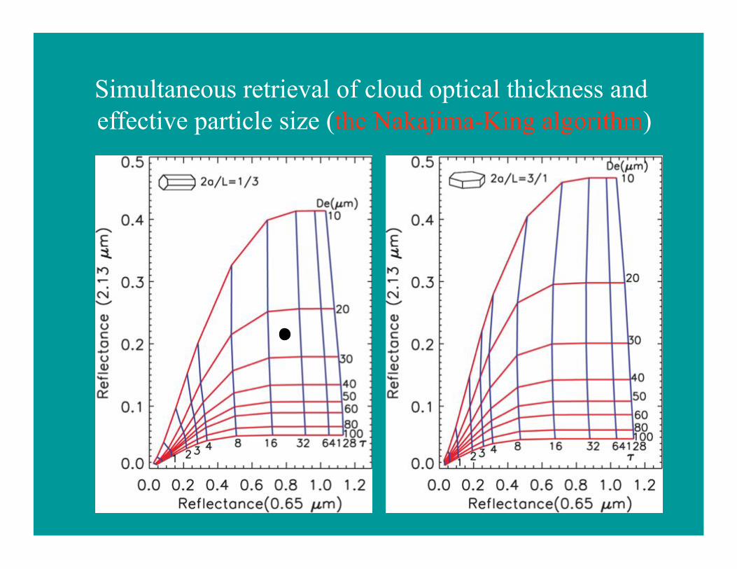
Simultaneous retrieval of cloud optical thickness and
effective particle size (the Nakajima-King algorithm)

Finite-difference time domain
(FDTD) simulation process ABC (Absorbing Boundary Condition)!
only scattered
fields
Plane parallel
Incident light is
applied on a
surface which
encloses the
particle

m
t
i
ri
=
=
!
!
!!
sin
sin
Snell’s Law
!! "=P
sdrikD ## 2)ˆexp(!
!"
#$%
&
+
+=
'
''
( cos10
0coscos
4
22Dk
Sd

Ice cloud models: MODIS Collection 004 vs 005

New habit: Droxtal
Courtesy of Andy Heymsfield
!!Predominant in the
uppermost portions of
cirrus clouds
!!20-Faced Polyhedron
12 isosceles trapezoid
6 rectangular
2 hexagonal
Ohtake (1970)

Field Campaign Location Instruments Number of PSDs
FIRE-1 (1986) Madison, WI 2D-C, 2D-P 246
FIRE-II (1991) Coffeyville, KS Replicator 22
ARM-IOP (2000) Lamont, OK 2D-C, 2D-P, CPI 390
TRMM KWAJEX (1999)
Kwajalein, Marshall Islands
2D-C, HVPS, CPI 418
CRYSTAL-FACE (2002)
Off coast of Nicaragua
2D-C, VIPS 41
Probe size ranges are: 2D-C, 40-1000 µm; 2D-P, 200-6400 µm; HVPS (High Volume
Precipitation Spectrometer), 200–6100 µm; CPI (Cloud Particle Imager), 20-2000 µm;
Replicator, 10-800 µm; VIPS (Video Ice Particle Sampler): 20-200 µm. "
Field Campaign Information
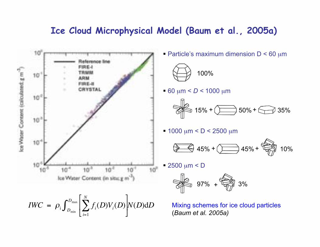
Ice Cloud Microphysical Model (Baum et al., 2005a)
Mixing schemes for ice cloud particles
(Baum et al. 2005a)
35%
10%
"! Particle’s maximum dimension D < 60 µm
100%
"! 60 µm < D < 1000 µm
15% 50%
"! 1000 µm < D < 2500 µm
45% 45%
"! 2500 µm < D
97% 3%
+ +
+ +
+
!
IWC = "i f i(D)Vi(D)i=1
N
#$
% &
'
( )
Dmin
Dmax* N(D)dD

Three-year Climatology of Ice Cloud Radiative Forcing
MYD08 level-3 daily 1º#1º $ !
MYD08 level-3 daily 1º#1º De!
daily 1º#1º cloud top pressure !
ISCCP!
Monthly ice cloud 1º#1º $ !
Monthly ice cloud 1º#1º De !
Monthly ice cloud top pressure !
Monthly ice cloud fraction !
AIRS level-3 monthly 1º#1º profile data ! LibRadtran!
(B."Mayer and A."Kylling, 2005)!
Our new parameterization!
Overcast-sky cloud forcing*!
Fscf=Fs-Fclear, Flcf=Fl-Fclear!
CLF= Fscf + Flcf!
Average-sky cloud forcing!
Fscf=A(Fs-Fclear), Flcf=A(Fl-Fclear)!CLF= Fscf + Flcf! (Hartmann et al. 2001)!
Monthly solar zenith angle !
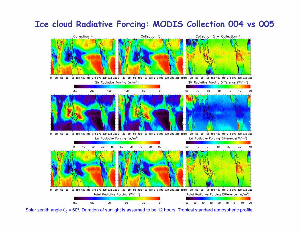
Solar zenith angle !0 = 60º, Duration of sunlight is assumed to be 12 hours, Tropical standard atmospheric profile
Ice cloud Radiative Forcing: MODIS Collection 004 vs 005

Improvements to Scattering models
•! New treatment of ray-spreading results in the removal of the term relating to delta-transmission energy at the forward scattering angle.
•! Improved the mapping algorithm: the single-scattering properties from the new algorithm smoothly transition to those from the conventional geometric optics method at large size parameters.
•! Semi-analytical method developed to improve the accuracy of the first-order scattering (diffraction and external reflection).
•! Semi-empirical method is developed to incorporate the edge effect on the extinction efficiency and the above/below-edge effects on the absorption efficiency.

Progress toward complex particle shapes
(Yang et al., 2008a)
(Tape, 1994;Xie et al., 2009) (Yang et al., 2008b)

Surface roughness
were observed for
single crystals and
polycrystalline ice
by using an
electronic
microscope.
Images adapted
from Cross, 1968!
The image of a rimed
column ice crystal
(adapted from Ono,
1969). The surface
roughness of this ice
crystal is evident.

As articulated by Mishchenko et al.
[1996] on the basis of the observations
reported in the literature, halos are not
often seen in the atmosphere and the
phase functions associated with ice
clouds might be featureless with no
pronounced halo peaks. One of the
mechanisms responsible for the
featureless phase function might be the
surface distortion or roughness of ice
crystals

Effect of particle surface roughness on retrievals: Ice cloud optical thickness and effective particle size
(Deeply rough)!

IHM model
Courtesy of
Dr. Jerome Riedi
Bulk scattering model
–!MODIS: Baum05 model (Baum, Yang and co-authors,
2005)
–!POLDER: IHM model (C.-Labonnote et al. 2000)
Differences between the MODIS and
POLDER ice cloud models
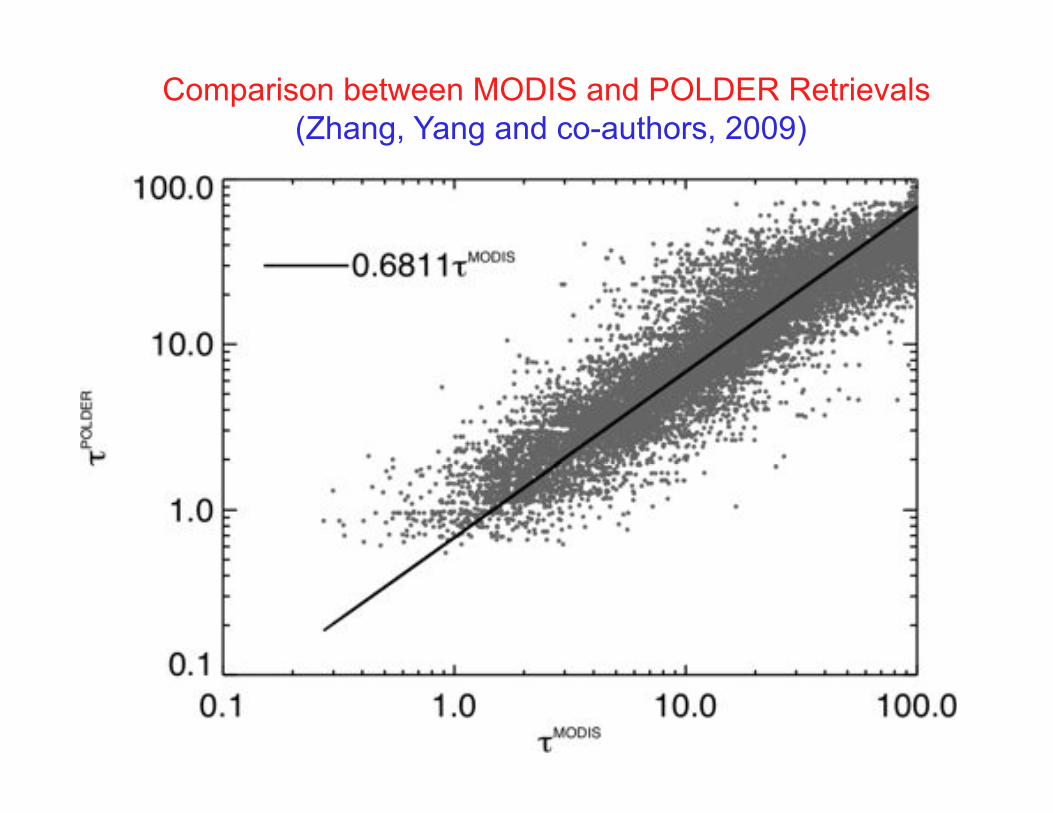
Comparison between MODIS and POLDER Retrievals
(Zhang, Yang and co-authors, 2009)
The false-color image
(Red: reflectance in
0.65-mm band; Green:
reflectance in 0.86-mm
band; Blue: Brightness
temperature of 11-mm
band after gray flopped)
of the Aqua MODIS
granule selected for
comparison. In the
image, ocean is dark,
land is green, low level
clouds appear yellowish
and high level clouds are
white or light blue. !

Asian Dust !
MODIS RGB (0.65µm, 0.55µm, 0.47µm) Image!
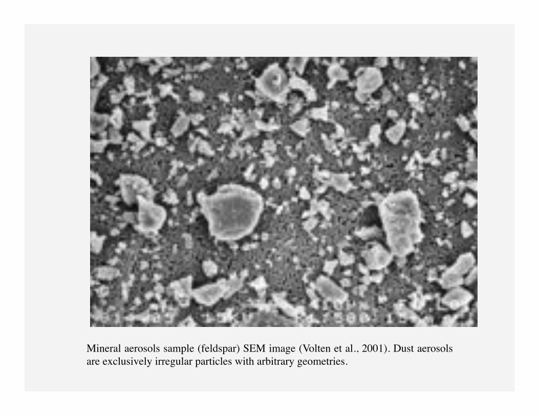
Mineral aerosols sample (feldspar) SEM image (Volten et al., 2001). Dust aerosols
are exclusively irregular particles with arbitrary geometries.!
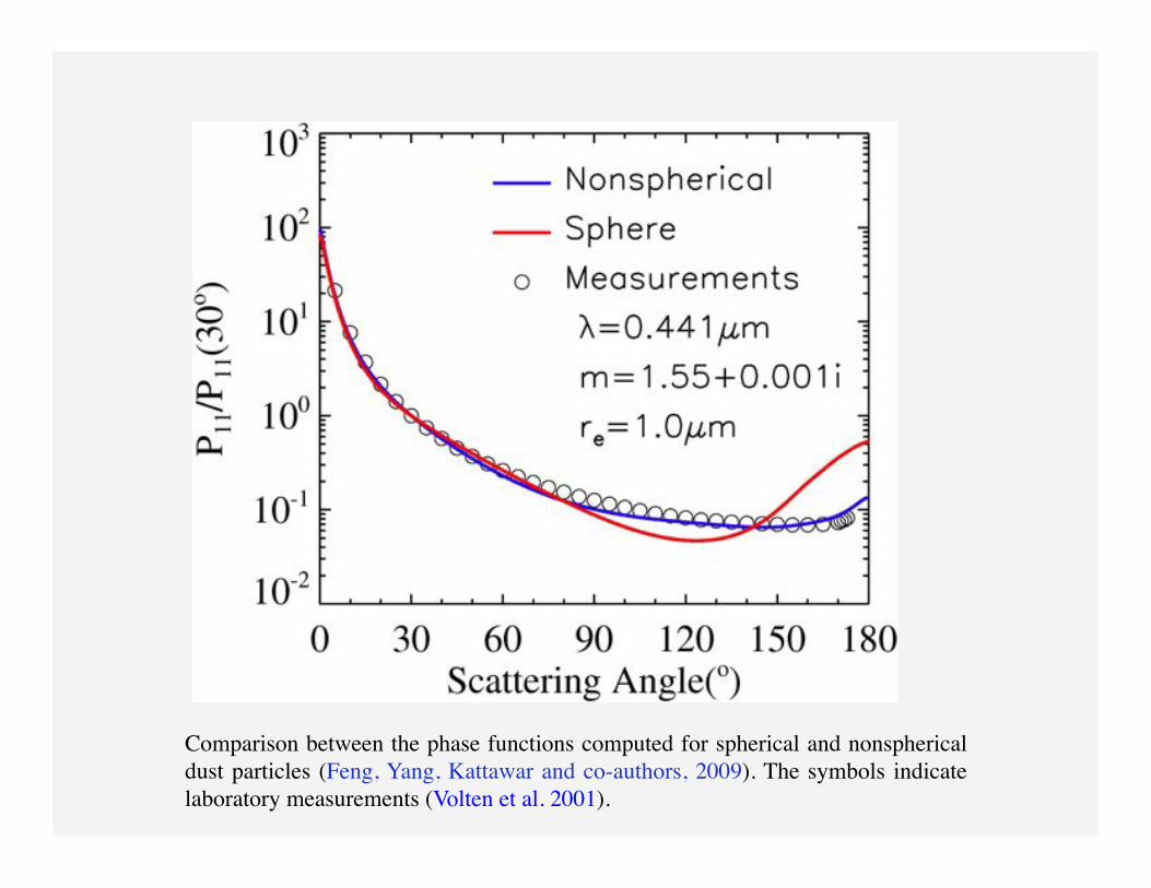
Comparison between the phase functions computed for spherical and nonspherical
dust particles (Feng, Yang, Kattawar and co-authors, 2009). The symbols indicate
laboratory measurements (Volten et al. 2001).!
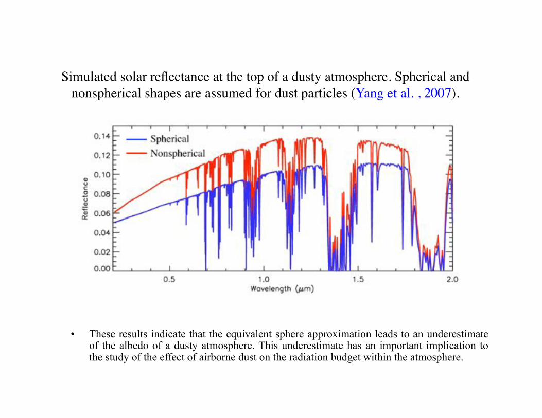
Simulated solar reflectance at the top of a dusty atmosphere. Spherical and
nonspherical shapes are assumed for dust particles (Yang et al. , 2007). !
•! These results indicate that the equivalent sphere approximation leads to an underestimate of the albedo of a dusty atmosphere. This underestimate has an important implication to the study of the effect of airborne dust on the radiation budget within the atmosphere.

MODIS RGB image on March 2, 2003, showing a dust plume over West Africa.
The area indicated by the small red box is used to retrieve dust AOD in the present
sensitivity study (Feng, Yang, Kattawar, Hsu, Tsay and Laszlo, 2009). !

Upper panels: the
retrieved dust AOD
based on the
nonspherical and
sphere models. !
Lower left panel:
retrieved dust AOD
based on the sphere
model versus those
based on the
nonspherical model. !
Lower right panel: the
relative differences of
the retrieved AOD (Feng, Yang, Kattawar,
Hsu, Tsay and Laszlo,
2009). !
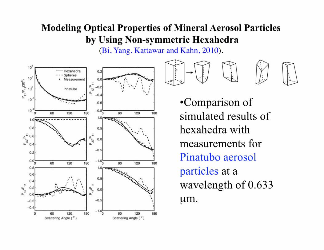
Modeling Optical Properties of Mineral Aerosol Particles
by Using Non-symmetric Hexahedra (Bi, Yang, Kattawar and Kahn, 2010). !
•!Comparison of
simulated results of
hexahedra with
measurements for
Pinatubo aerosol
particles at a
wavelength of 0.633
µm.
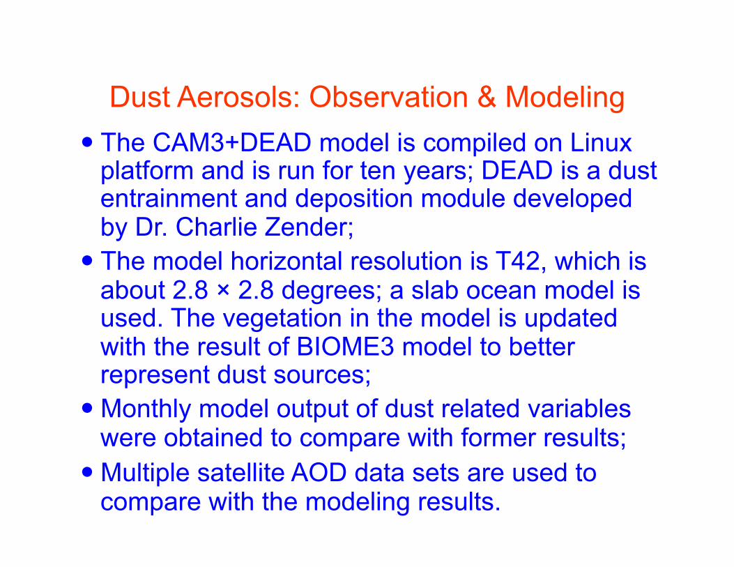
Dust Aerosols: Observation & Modeling !!The CAM3+DEAD model is compiled on Linux
platform and is run for ten years; DEAD is a dust entrainment and deposition module developed by Dr. Charlie Zender;
!!The model horizontal resolution is T42, which is about 2.8 ! 2.8 degrees; a slab ocean model is used. The vegetation in the model is updated with the result of BIOME3 model to better represent dust sources;
!!Monthly model output of dust related variables were obtained to compare with former results;
!!Multiple satellite AOD data sets are used to compare with the modeling results.
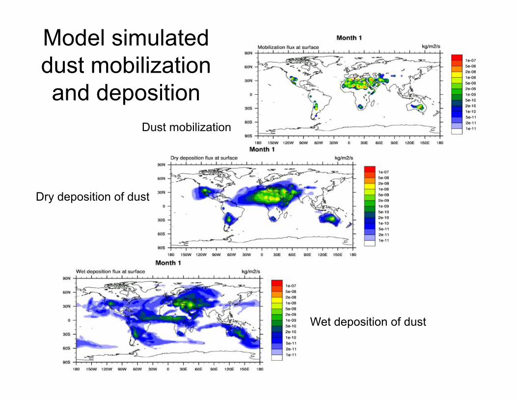
Model simulated
dust mobilization
and deposition
Dust mobilization
Dry deposition of dust
Wet deposition of dust

Modeled and Observed AOD - Spring

Modeled and Observed AOD - Fall
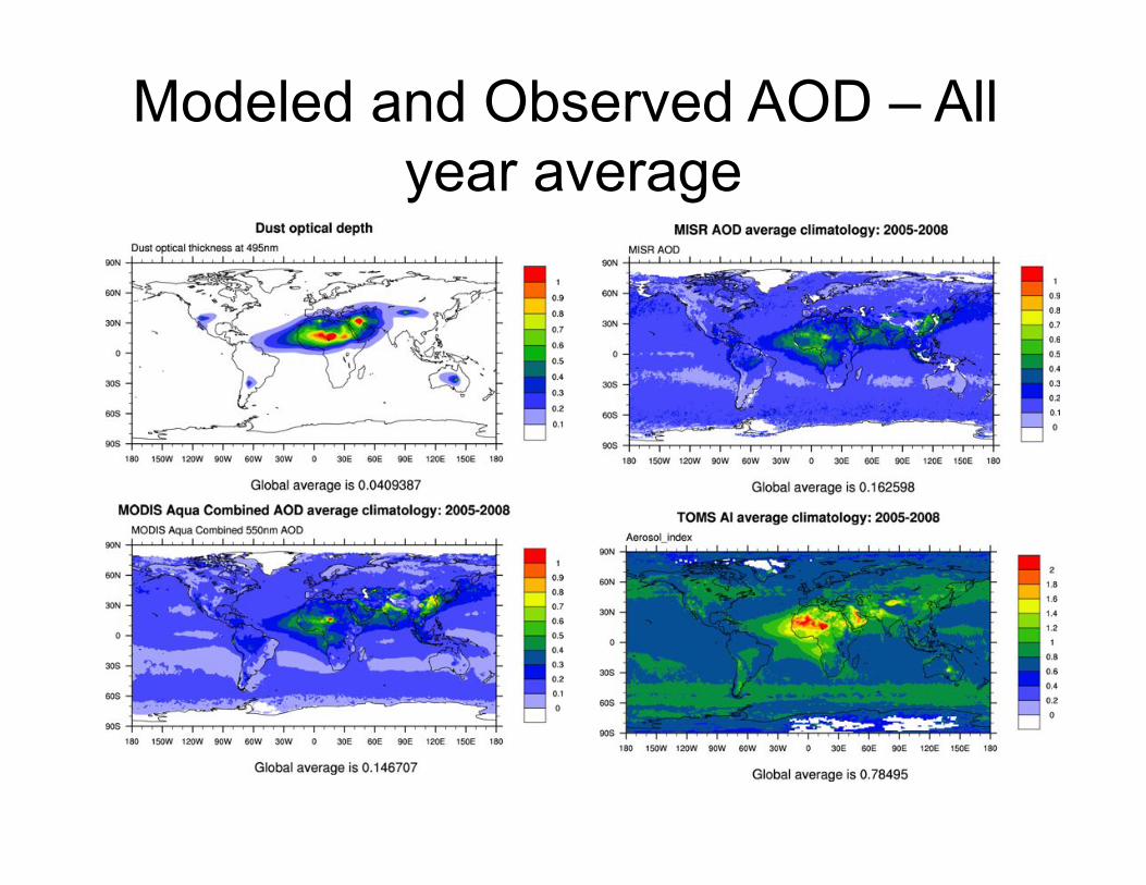
Modeled and Observed AOD – All
year average

Dust radiative forcing
Fig. Simulated dust radiative effect: difference in Short-wave and Long-
wave radiative flux at TOA and SFC in dust-on and dust-off cases

“Thin” Cirrus clouds •! “Thin” cirrus clouds are defined here as being those not
detected by the operational MODIS cloud mask, corresponding
to an optical depth value of approximately 0.3 or smaller, but
are detectable in terms of the cirrus reflectance product based
on the MODIS 1.375-!m channel;
•! Our preliminary results show that thin cirrus clouds were
present in more than 40% of the pixels flagged as “clear-sky”
by the operational MODIS cloud mask algorithm;
•! The present study shows positive and negative net forcings at
the top of the atmosphere (TOA) and at the surface,
respectively. The positive (negative) net forcing at TOA (the
surface) is due to the dominance of longwave (shortwave)
forcing. Both the TOA and surface forcings are in a range of
0-20 Wm-2, depending on the optical depths of thin cirrus
clouds.

Cross-section of color-coded raw backscatter signal from the LITE 532 nm channel over the western!
Pacific Ocean. White indicates dense clouds or the ocean surface return, dark blue indicates clean
atmosphere, reds and greens generally indicate aerosols. Laminar cirrus is seen at an altitude of 17
km. (Winker and Trepte, 1998).

Optical depths of tropical
thin cirrus clouds for the
pixels flagged as “clear-
sky” by MODIS for
boreal (a) spring, (b)
summer, (c) autumn, and
(d) winter (Lee, Yang and
co-authors, 2009)
Subvisible
cirrus clouds

(a)!Histograms of optical
depth of thin cirrus clouds
retrieved between
latitudes 30°S and 30°N
for each of boreal seasons.
(b)! Cumulative fractions of
optical depth of thin cirrus
clouds for each of boreal
seasons.
Lee, Yang and co-
authors (2009)
Subvisible cirrus clouds
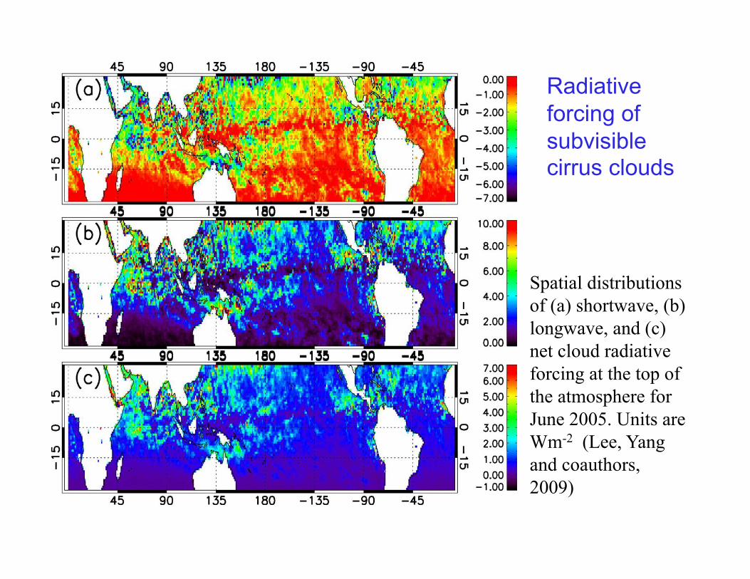
Spatial distributions
of (a) shortwave, (b)
longwave, and (c)
net cloud radiative
forcing at the top of
the atmosphere for
June 2005. Units are
Wm-2 (Lee, Yang
and coauthors,
2009)
Radiative
forcing of
subvisible cirrus clouds

Summary
•! Research with MODIS cloud products:
- comparisons of global properties with NCAR CAM3
- comparisons of MODIS with POLDER and CALIPSO
- collaboration with other groups working with MODIS data independently
•! Use of MODIS cloud products to investigate tropical equatorial waves
•! Improvements in deriving the single-scattering properties of aerosols and ice clouds:
- new habits: hollow bullet rosettes, aggregates of plates
- improved computational models
- ice models being used by many EOS sensor teams
- dust models include nonspherical particles
•! We studied the distribution and radiative forcing of tropical “thin” cirrus clouds.


![An improved limited area model for describing the dust ... · microchemical, and, hence, optical and radiative properties of clouds [Charlson et al., 1991]. Also, combined with certain](https://img.pdfslide.us/doc/110x75/602a82ecbf600e2389669fd1/an-improved-limited-area-model-for-describing-the-dust-microchemical-and-hence.jpg)