Embed Size (px)
Citation preview

Gas and dust in the Magellanicclouds
A Thesis
Submitted for the Award of the Degree of
Doctor of Philosophy in Physics
To
Mangalore University
by
Ananta Charan Pradhan
Under the Supervision of
Prof. Jayant Murthy
Indian Institute of AstrophysicsBangalore - 560 034
India
April 2011

Declaration of Authorship
I hereby declare that the matter contained in this thesis is the result of the inves-
tigations carried out by me at Indian Institute of Astrophysics, Bangalore, under
the supervision of Professor Jayant Murthy. This work has not been submitted for
the award of any degree, diploma, associateship, fellowship, etc. of any university
or institute.
Signed:
Date:
ii

Certificate
This is to certify that the thesis entitled ‘Gas and Dust in the Magellanic
clouds’ submitted to the Mangalore University by Mr. Ananta Charan Pradhan
for the award of the degree of Doctor of Philosophy in the faculty of Science, is
based on the results of the investigations carried out by him under my supervi-
sion and guidance, at Indian Institute of Astrophysics. This thesis has not been
submitted for the award of any degree, diploma, associateship, fellowship, etc. of
any university or institute.
Signed:
Date:
iii

Dedicated to my parents
=========================================
Sri. Pandab Pradhan and Smt. Kanak Pradhan=========================================

Acknowledgements
It has been a pleasure to work under Prof. Jayant Murthy. I am grateful to him for
giving me full freedom in research and for his guidance and attention throughout
my doctoral work inspite of his hectic schedules. I am indebted to him for his
patience in countless reviews and for his contribution of time and energy as my
guide in this project.
I would like to express my special thanks to Dr. Amit Pathak, Dr. Rekhesh Mohan
and Dr. N. V. Sujatha who stood with me in frustrating period of my research
career, encouraged me patiently and extended their helping hand whenever it was
needed. I thank to our group members, Rita, Shalima, Abhay, Veena, and others
for many useful discussions on the subject during our group meetings almost on
every Tuesday.
I am thankful to the Director of Indian Institute of Astrophysics, Prof. Siraj
Hassan for giving me the opportunity to work in this institute and providing
all the facilities required for my research work. I thank to the Dean Academic,
Prof. Harish Bhatt, the BGS chair, Prof. S. K. Saha, the BGS Secretary, Prof.
R. Ramesh and all the members of the Board of Graduate Studies for providing
the necessary facilities to work comfortably in IIA. I thank Prof. B. P. Das, Prof.
Dipankar Banerjee, Dr. Gajendra Pandey, Dr. Ravinder Banyal, Prof. Annapurni
Subramanium, Prof. G. C. Anupama, Dr. Sivarani Thirupathi, Prof. Rajat
Chaudhuri and Dr. Muthumariappan for their advice and fruitful discussions. I
thank Dr. Christina Birdie, Mr. B. S. Mohan, Mr. Prabhahar and the other staffs
of the library for assisting me in getting the required books and journals in time.
I thank Dr. Baba Varghese, Mr. Fayaz and Mr. Ashok for their help in computer
related problems.
It is my pleasure to thank my friends Tapan bhai, Bharat, Girjesh, Rumpa, Ramya,
Veeresh, Amit, Nataraj, Chanduri, Krishna, Vigeesh, Blesson, Nagaraj, Uday,
Malay da, Sam, Arya, Pradeep, Sajal, Jyotirmaya, Avijeet, Drisya, Indu, Ramya
P., Sinduja, Ratnakumar, Prasanth, Dinesh, Hema, Arun, Suresh, Vineeth, Anan-
tha, Smitha, Shashi, Vyas, Roopashree, Vaidehi, Narshi, Sagar, Subham and many
v

more of my juniors with whom I have shared a lot of funs and laughs apart from
the various scientific discussions throughout my stay in IIA.
I thank administrative officer Dr. Kumaresan, personnel officer Mr. Narasimha
Raju and the administrative staff who are cooperative making the administrative
related issues very smooth. I thank Mr. Mohan Kumar, M. G. Mohan, Rajen-
dran, John and Sandip who took good care making our stay in Bhaskara extremly
gratified.
Its my pleasure to thank my nearer and dearer friends Babuni, Nandi, Ramani,
Kamadev, Rudra bhai, Saumya bhai, Madhusmita didi, Kunmun didi, Subrat bhai
and Papu bhai who are with me in pros and cons of my life giving me a lot of
confidence and self belief. I would like to thank my friends from IISc, Sankarsan,
Pratap, Chakrapani, Sabya, Khatei bhai, Sudhansu bhai, Bapina bhai and Rama
bhai for providing joyful atmospheres by arranging weekend cricket matches, bad-
minton tournaments, picnics and champagne parties which were essential to cherish
the weekend.
I am extremely thankful to Prof. Balakrishna and Prof. Dharmaprakash of depart-
ment of physics for their suggestions during registration, conduction of colloquium
and other University formalities. I sincerely thank to the Mrs Anita and other ad-
ministrative staffs of the Mangalore University for helping me at all stages of
communications and official procedures.
Most especially, I express my gratitudes to my parents and many many many .. ..
thanks to my wife Madhulita Das (Rinky) for everything.

List of Publications
1. “Far Ultraviolet Diffuse emission from the Large Magellanic Cloud”, Ananta
C. Pradhan, Amit Pathak, & Jayant Murthy, 2010, ApJ Letters, 718, 141
– 144.
2. “Survey of O VI absorption in the Large Magellanic Cloud”, Amit Pathak,
Ananta C. Pradhan, Sujatha, N. V. & Jayant Murthy, 2010, MNRAS,
412, 1105 – 1122.
3. “Observations of Far Ultraviolet Diffuse Emission from the Small Magel-
lanic Cloud”, Ananta C. Pradhan, Jayant Murthy & Amit Pathak, 2011,
ApJ,743, 80.
4. “Properties of O VI emitting symbiotic stars in the Small Magellanic Cloud”,
Amit Pathak, Robin Shelton, Ananta C. Pradhan & Jayant Murthy, sub-
mitted in MNRAS.
5. “New light on star birthplace”, Ananta C. Pradhan, Amit Pathak, &
Jayant Murthy, Nature India, doi:10.1038/nindia.2010.96; Published on-
line.
6. “Far Ultraviolet Characteristics of the Interstellar Medium of the Magel-
lanic Clouds”, Amit Pathak, Ananta C. Pradhan & Jayant Murthy, Book
Chapter, Nova Science Publishers, Hauppauge, NY 11788-3619, USA.
vii

Presentations
1. Formation of Interstellar Dust.
Astrosat meeting, 2007, Christ University, Bangalore, India.
2. Data Analysis by Aladin and Simbad.
Astrosat meeting, 2007, Christ University, Bangalore, India.
3. Formation of Interstellar Dust.
Young Astronomer Meet, 2007, IIA, Bangalore, India.
4. Ultraviolet Absorption Line Analysis of a O type star: BD602522.
9th COSPAR Capacity building Workshop on Space Optical and UV Astron-
omy, 2008, Kuala Lumpur, Malaysia.
5. Extinction Mapping through Broad Band Photometry.
Young Astronomer Meet, 2009, IIT, Kharagpur, India.
6. Extinction Mapping through Broad Band Photometry.
Dust Workshop, Vainu Bappu Observatory, Kavalur, India, 2009.
7. Far Ultraviolet Diffuse emission from the Large Magellanic Cloud.
National Space Science Symposium, 2010, Saurashtra University, Rajkot,
India.
8. Far Ultraviolet Diffuse emission from the Large Magellanic Cloud.
Wittfest: Origins & Evolution of Dust, 2010, University of Toledo, USA.
9. Observations of Far Ultraviolet Diffuse emission from the Small Magellanic
Cloud.
Astronomical Society of India, 2011, Pt. Ravishankar Shukla University,
Raipur, India.
viii
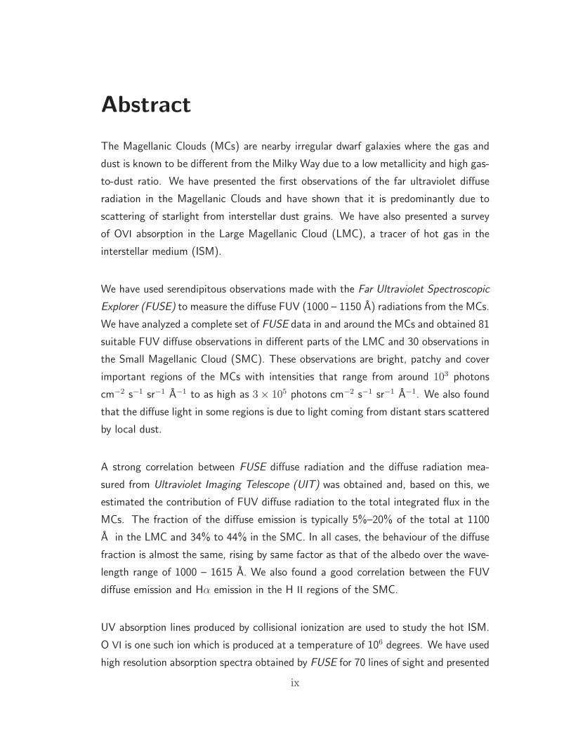
Abstract
The Magellanic Clouds (MCs) are nearby irregular dwarf galaxies where the gas and
dust is known to be different from the Milky Way due to a low metallicity and high gas-
to-dust ratio. We have presented the first observations of the far ultraviolet diffuse
radiation in the Magellanic Clouds and have shown that it is predominantly due to
scattering of starlight from interstellar dust grains. We have also presented a survey
of OVI absorption in the Large Magellanic Cloud (LMC), a tracer of hot gas in the
interstellar medium (ISM).
We have used serendipitous observations made with the Far Ultraviolet Spectroscopic
Explorer (FUSE) to measure the diffuse FUV (1000 – 1150 A) radiations from the MCs.
We have analyzed a complete set of FUSE data in and around the MCs and obtained 81
suitable FUV diffuse observations in different parts of the LMC and 30 observations in
the Small Magellanic Cloud (SMC). These observations are bright, patchy and cover
important regions of the MCs with intensities that range from around 103 photons
cm−2 s−1 sr−1 A−1 to as high as 3 × 10⁵ photons cm−2 s−1 sr−1 A−1. We also found
that the diffuse light in some regions is due to light coming from distant stars scattered
by local dust.
A strong correlation between FUSE diffuse radiation and the diffuse radiation mea-
sured from Ultraviolet Imaging Telescope (UIT) was obtained and, based on this, we
estimated the contribution of FUV diffuse radiation to the total integrated flux in the
MCs. The fraction of the diffuse emission is typically 5%–20% of the total at 1100
A in the LMC and 34% to 44% in the SMC. In all cases, the behaviour of the diffuse
fraction is almost the same, rising by same factor as that of the albedo over the wave-
length range of 1000 – 1615 A. We also found a good correlation between the FUV
diffuse emission and Hα emission in the H II regions of the SMC.
UV absorption lines produced by collisional ionization are used to study the hot ISM.
O VI is one such ion which is produced at a temperature of 106 degrees. We have used
high resolution absorption spectra obtained by FUSE for 70 lines of sight and presented
ix

a wide survey of O VI column density measurements for the LMC. The column density
varies from a minimum of log N(O VI) = 13.72 atoms cm−2 to a maximum value of
log N(O VI) = 14.57 atoms cm−2. We found a high abundance of O VI in both active
(superbubbles) and inactive regions of the LMC. The abundance and properties of
OVI absorption are similar in the LMC and the Milky Way (MW) despite the fact that
the LMC has lower metallicity than the MW. O VI absorption in the LMC does not
correlate with Hα (warm gas) or X-ray (hot gas) but correlates with X-ray emission in
the 30 Doradus region, a star forming region of the LMC and decreases with increase in
angular distance from the star cluster R136 suggesting that the strength of the stellar
wind from the central cluster decreases outwards.
Contents
Declaration of Authorship ii
Certificate iii
Acknowledgements v
List of Publications vii
Presentations viii
Abstract ix
List of Figures xv
List of Tables xvii
Abbreviations xix
1 Interstellar Medium 1
1.1 History of the ISM . . . . . . . . . . . . . . . . . . . . . . . . . . . 2
1.2 ISM Star Cycle . . . . . . . . . . . . . . . . . . . . . . . . . . . . . 2
1.3 Gas Components of the ISM . . . . . . . . . . . . . . . . . . . . . . 3
1.3.1 Molecular Gas . . . . . . . . . . . . . . . . . . . . . . . . . . 3
1.3.2 Atomic Gas . . . . . . . . . . . . . . . . . . . . . . . . . . . 4
1.3.3 Ionized Gas . . . . . . . . . . . . . . . . . . . . . . . . . . . 5
1.4 Dust . . . . . . . . . . . . . . . . . . . . . . . . . . . . . . . . . . . 7
1.4.1 Extinction . . . . . . . . . . . . . . . . . . . . . . . . . . . . 8
1.4.2 The Average Extinction Curve . . . . . . . . . . . . . . . . . 11
1.4.3 Size Distribution of Dust Grain . . . . . . . . . . . . . . . . 12
xi

Contents xii
1.4.4 The Dust to Gas Ratio . . . . . . . . . . . . . . . . . . . . . 13
1.4.5 Dust Absorption and Emission . . . . . . . . . . . . . . . . . 14
1.4.6 Temperature of Dust Grain . . . . . . . . . . . . . . . . . . 15
1.4.7 Polarization . . . . . . . . . . . . . . . . . . . . . . . . . . . 18
1.4.8 Dust Scattering . . . . . . . . . . . . . . . . . . . . . . . . . 19
1.5 Heating Mechanisms in the ISM . . . . . . . . . . . . . . . . . . . . 21
1.5.1 Photoionization . . . . . . . . . . . . . . . . . . . . . . . . . 22
1.5.2 Cosmic Rays . . . . . . . . . . . . . . . . . . . . . . . . . . 22
1.5.3 X-Rays . . . . . . . . . . . . . . . . . . . . . . . . . . . . . . 23
1.5.4 Heating by Photodissociation of Molecules . . . . . . . . . . 24
1.5.5 Chemical Heating . . . . . . . . . . . . . . . . . . . . . . . . 25
1.5.6 Photo-electric Heating . . . . . . . . . . . . . . . . . . . . . 25
1.5.7 Grain-Gas Heating . . . . . . . . . . . . . . . . . . . . . . . 26
1.5.8 Heating by Macroscopic Processes . . . . . . . . . . . . . . . 26
1.6 Cooling Mechanisms in the ISM . . . . . . . . . . . . . . . . . . . . 27
1.6.1 Molecular Cooling . . . . . . . . . . . . . . . . . . . . . . . 27
1.6.2 Cooling by Resonance and Metastable lines . . . . . . . . . 28
1.6.3 Cooling by Dust . . . . . . . . . . . . . . . . . . . . . . . . . 29
1.6.4 Fine Structure Line Cooling . . . . . . . . . . . . . . . . . . 29
1.6.5 Recombination . . . . . . . . . . . . . . . . . . . . . . . . . 29
1.6.6 Bremsstrahlung . . . . . . . . . . . . . . . . . . . . . . . . . 30
2 Diffuse Background Radiation in the Ultraviolet: Observationsand Data Reduction 31
2.1 Diffuse UV Background . . . . . . . . . . . . . . . . . . . . . . . . 31
2.2 Components of the Diffuse UV Radiation . . . . . . . . . . . . . . . 32
2.3 Cosmic UV Background . . . . . . . . . . . . . . . . . . . . . . . . 33
2.4 Far Ultraviolet Spectroscopic Explorer . . . . . . . . . . . . . . . . 36
2.4.1 FUSE Instrument . . . . . . . . . . . . . . . . . . . . . . . . 38
2.4.2 FUSE Apertures . . . . . . . . . . . . . . . . . . . . . . . . 38
2.4.3 Data Reduction Pipeline . . . . . . . . . . . . . . . . . . . . 39
2.4.4 FUSE Observations . . . . . . . . . . . . . . . . . . . . . . . 39
2.5 Ultraviolet Imaging Telescope (UIT) . . . . . . . . . . . . . . . . . . 44
2.5.1 UIT Instrument . . . . . . . . . . . . . . . . . . . . . . . . . 44
2.5.2 UIT Observations of the MCs . . . . . . . . . . . . . . . . . 44
2.5.3 Conversion of UIT flux to Photon units . . . . . . . . . . . . 44
2.6 Stellar Radiation Field Model . . . . . . . . . . . . . . . . . . . . . 45
2.7 Calculation of Errors in Diffuse Fraction . . . . . . . . . . . . . . . 46
3 Far Ultraviolet Diffuse Emission from the Large Magellanic Cloud 47
3.1 Introduction . . . . . . . . . . . . . . . . . . . . . . . . . . . . . . . 47
3.2 Ultraviolet Observations of the LMC . . . . . . . . . . . . . . . . . 50
3.3 FUV Diffuse Emissions in the LMC . . . . . . . . . . . . . . . . . . 52

Contents xiii
3.4 FUSE – UIT Correlation . . . . . . . . . . . . . . . . . . . . . . . . 53
3.4.1 Calculation of Diffuse Fraction . . . . . . . . . . . . . . . . . 54
3.5 Discussion . . . . . . . . . . . . . . . . . . . . . . . . . . . . . . . . 56
3.6 Conclusions . . . . . . . . . . . . . . . . . . . . . . . . . . . . . . . 57
4 Far Ultraviolet Diffuse Emission from the Small Magellanic Cloud 61
4.1 Introduction . . . . . . . . . . . . . . . . . . . . . . . . . . . . . . . 61
4.2 FUV Diffuse Emission from the SMC . . . . . . . . . . . . . . . . . 63
4.2.1 Diffuse Fraction . . . . . . . . . . . . . . . . . . . . . . . . . 66
4.3 Correlation with the Hα Emission . . . . . . . . . . . . . . . . . . . 69
4.4 Conclusion . . . . . . . . . . . . . . . . . . . . . . . . . . . . . . . . 70
5 Survey of OVI in the Large Magellanic Cloud 75
5.1 Introduction . . . . . . . . . . . . . . . . . . . . . . . . . . . . . . . 75
5.2 Observations and Data analysis . . . . . . . . . . . . . . . . . . . . 78
5.2.1 FUSE Data Analysis and Possible Contamination . . . . . . 78
5.2.2 Measurement of O VI Column Densities . . . . . . . . . . . 83
5.3 Distribution and Properties of O VI in the LMC . . . . . . . . . . . 84
5.3.1 Abundance and Linewidth of O VI . . . . . . . . . . . . . . 84
5.3.2 Comparison with the MW and the SMC . . . . . . . . . . . 86
5.3.3 Comparison with X-ray and Hα . . . . . . . . . . . . . . . . 88
5.4 O VI in superbubbles of the LMC . . . . . . . . . . . . . . . . . . . 90
5.5 Properties of O VI in 30 Doradus . . . . . . . . . . . . . . . . . . . 93
5.6 Summary & Conclusions . . . . . . . . . . . . . . . . . . . . . . . . 95
6 Summary & Conclusions 111
6.1 Summary . . . . . . . . . . . . . . . . . . . . . . . . . . . . . . . . 111
6.1.1 Future Plans . . . . . . . . . . . . . . . . . . . . . . . . . . 114
Bibliography 117


List of Figures
1.1 Extinction Curve . . . . . . . . . . . . . . . . . . . . . . . . . . . . 11
1.2 Dust Emission Spectrum . . . . . . . . . . . . . . . . . . . . . . . . 14
1.3 Dust map . . . . . . . . . . . . . . . . . . . . . . . . . . . . . . . . 15
2.1 Distribution diffuse UV over the sky . . . . . . . . . . . . . . . . . 34
2.2 Schematic of the FUSE Instrument . . . . . . . . . . . . . . . . . . 37
2.3 Image of 1A Detector Segment . . . . . . . . . . . . . . . . . . . . . 41
2.4 Profile of LiF LWRS aperture . . . . . . . . . . . . . . . . . . . . . 42
2.5 A Sample Diffuse Spectrum . . . . . . . . . . . . . . . . . . . . . . 43
3.1 A radio image of MCs . . . . . . . . . . . . . . . . . . . . . . . . . 48
3.2 LMC R-band image . . . . . . . . . . . . . . . . . . . . . . . . . . . 51
3.3 FUSE–FUSE Correlation . . . . . . . . . . . . . . . . . . . . . . . . 53
3.4 Correlation between the FUSE and the UIT . . . . . . . . . . . . . 54
3.5 Diffuse fraction against Wavelength . . . . . . . . . . . . . . . . . . 56
4.1 SMC 160 micron image . . . . . . . . . . . . . . . . . . . . . . . . . 62
4.2 SMC 160 micron image . . . . . . . . . . . . . . . . . . . . . . . . . 64
4.3 Correlation between the FUSE and the UIT . . . . . . . . . . . . . 65
4.4 Variation of diffuse fraction against wavelength for different UITregions of the SMC. . . . . . . . . . . . . . . . . . . . . . . . . . . . 67
4.5 Comparison of FUV diffuse fraction of the LMC and the SMC. . . . 68
4.6 Correlation of the FUV diffuse surface brightness with the Hα flux . 70
5.1 Sample FUSE spectra showing O VI absorption . . . . . . . . . . . 76
5.2 O VI distribution in LMC . . . . . . . . . . . . . . . . . . . . . . . 77
5.3 Complexity of fitting the stellar continuum. . . . . . . . . . . . . . 79
5.4 Model for H2 absorption . . . . . . . . . . . . . . . . . . . . . . . . 82
5.5 Hα image of the LMC . . . . . . . . . . . . . . . . . . . . . . . . . 89
5.6 O VI column density (log N(O VI)) vs. log relative Hα surfacebrightness . . . . . . . . . . . . . . . . . . . . . . . . . . . . . . . . 90
5.7 O VI column density log N(O VI) vs. log relative X-ray surfacebrightness . . . . . . . . . . . . . . . . . . . . . . . . . . . . . . . . 91
5.8 O VI column density (log N(O VI)) vs. distance from the the centreof the star cluster R136 of 30 Doradus . . . . . . . . . . . . . . . . 93
xv

List of Figures xvi
5.9 O VI column density (log N(O VI)) vs. log relative X-ray surfacebrightness for 30 Doradus region . . . . . . . . . . . . . . . . . . . . 94
5.10 Normalized O VI absorption profiles for the 70 lines of sight. . . . . 102

List of Tables
1.1 Components of the Interstellar Medium . . . . . . . . . . . . . . . . 3
2.1 Bands Used for Extraction of Diffuse Emission . . . . . . . . . . . . 43
3.1 Calculation of Far Ultraviolet Diffuse Fraction (DF) for the FUSE1B1 (1117 A) band. . . . . . . . . . . . . . . . . . . . . . . . . . . . 55
3.2 Details of the FUSE observations in the LMC. . . . . . . . . . . . . 58
4.1 Details of FUSE observations in the SMC. . . . . . . . . . . . . . . 72
5.1 Log of FUSE observations for the 70 targets in the LMC. . . . . . . 103
5.2 Equivalent widths and column densities with corresponding velocitylimits over which the integration is performed for O VI absorptionin the LMC. . . . . . . . . . . . . . . . . . . . . . . . . . . . . . . . 106
5.3 O VI column densities in the superbubbles (SB) of the LMC. . . . . 109
xvii


Abbreviations
ApJ Astrophysical Journal
ApJL Astrophysical Journal Letters
ApJS Astrophysical Journal Supplement Series
A&A Astronomy & Astrophysics
MNRAS Monthly Notices of the Royal Astronomical Society
AJ Astronomical Journal
PASJ Publications of the Astronomical Society of Japan
PASP Publications of the Astronomical Society of Pacific
BASI Bulletin of the Astronomical Society of India
BAIN Bulletin of the Astronomical Institutes of the Netherlands
A&SS Astrophysics and Space Science
ARA&A Annual Review of Astronomy & Astrophysics
A&AS Astronomy & Astrophysics Supplement Series
SSR Space Science Reviews
IAU International Astronomical Union
xix


Chapter 1
Interstellar Medium
Interstellar medium (ISM) is the region between the stars and is composed of 99%
gas (atoms, molecules, ions, and electrons) and 1% dust by mass. Of the 99% gas
about 89% is hydrogen, 9% is helium and 2% are metals (elements heavier than
hydrogen and helium). Apart from the gas and dust, cosmic rays and magnetic
fields are also components of the ISM. The ISM has very low density with an
average density of 1 atom per cubic centimeter (cc) although it fluctuates up to
a million atoms per cc in some regions, where as the best man made vacuum has
1012 atoms per cc. The total mass of gas and dust in the ISM is about 10% –
15% of the total mass of the visible matter in the Milky Way (MW). Information
about the ISM is obtained by the spectroscopic analysis of the lines produced by
the atoms, ions, and molecules present in it. Although it does not shine brightly
like stars, it does play an important role in regulating the physical and chemical
processes of the Galaxy. The constituents of the ISM and their interactions in our
Galaxy have been described in an excellent review by Ferriere (2001).
1

Chapter 1: Interstellar Medium 2
1.1 History of the ISM
In the late eighteenth century, Sir William Herschel noticed dark patches in be-
tween the arbitrarily distributed stars which he described as ‘holes in the heavens’.
The deep night sky photographic surveys of Edward Barnard showed many more
such dark regions with variety of shapes and sizes. Then it was realized that these
dark regions or holes are due to dark clouds of interstellar matter obscuring the
stars behind them. The first observational evidence of existence of the ISM came
from the discovery of Hartmann (1904) in which he found stationary absorption
lines of Ca II (3934 A) in the spectrum of the spectroscopic binary star δ Orionis.
To his surprise, he found that these lines were not undergoing periodically varying
Doppler shift like broad absorption lines of stars. This fact evinced that these lines
must have been produced by the interstellar matter but not by the stars. Further
more such stationary lines were detected in spectra of bright O and B type stars
revealing presence of several intervening clouds in the line of sight (Beals 1936;
Adams 1949). Later on Trumpler (1930) provided the evidence for the existence
of interstellar absorption and scattering by the pervasive ISM which led to the
confirmation of the presence of interstellar dust.
1.2 ISM Star Cycle
The structure of the ISM is determined by the interplay between massive stars
and the ISM. The stars are formed from the coldest and densest molecular gas
in the ISM, where the conditions are favorable for the formation of stars. The
matter inside the star undergoes a series of thermonuclear reactions, which enriches
heavy elements in it. These elements are returned to the ISM through cataclysmic
processes like powerful stellar winds, supernova explosions or through mass ejection
in the red giant phase of relatively less mass stars. By these methods, the expulsion
of matter from the star is accompanied by release of huge amount of energy. This
energy generates turbulent motions that stirs the ISM to maintain its hetergenous
structure and also causes the heating of the ISM. Under suitable condition of
temperature and pressure, the ISM forms molecular clouds that are prone to star
Chapter 1: Interstellar Medium 3
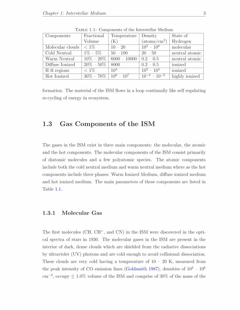
Table 1.1: Components of the Interstellar Medium
Components Fractional Temperature Density State ofVolume (K) (atoms/cm3) Hydrogen
Molecular clouds < 1% 10 – 20 102 – 106 molecularCold Neutral 1% – 5% 50 – 100 20 – 50 neutral atomicWarm Neutral 10% – 20% 6000 – 10000 0.2 – 0.5 neutral atomicDiffuse Ionized 20% – 50% 8000 0.2 – 0.5 ionizedH II regions < 1% 104 102 – 104 ionizedHot Ionized 30% – 70% 106 – 107 10−4 – 10−2 highly ionized
formation. The material of the ISM flows in a loop continually like self regulating
re-cycling of energy in ecosystem.
1.3 Gas Components of the ISM
The gases in the ISM exist in three main components: the molecular, the atomic
and the hot components. The molecular components of the ISM consist primarily
of diatomic molecules and a few polyatomic species. The atomic components
include both the cold neutral medium and warm neutral medium where as the hot
components include three phases: Warm Ionized Medium, diffuse ionized medium
and hot ionized medium. The main parameters of these components are listed in
Table 1.1.
1.3.1 Molecular Gas
The first molecules (CH, CH+, and CN) in the ISM were discovered in the opti-
cal spectra of stars in 1930. The molecular gases in the ISM are present in the
interior of dark, dense clouds which are shielded from the radiative dissociations
by ultraviolet (UV) photons and are cold enough to avoid collisional dissociation.
These clouds are very cold having a temperature of 10 – 20 K, measured from
the peak intensity of CO emission lines (Goldsmith 1987), densities of 102 – 106
cm−3, occupy ≤ 1.0% volume of the ISM and comprise of 30% of the mass of the

Chapter 1: Interstellar Medium 4
ISM. Most of them are gravitationally bound and are the sites of star formation.
The wealth of information on the spatial distribution, physics and chemistry of
molecules in the ISM were accumulated after the vast advancement of UV astron-
omy, particularly by the launch of Copernicus Satellite, International Ultraviolet
Explorer (IUE), Far Ultraviolet Spectroscopic Explorer (FUSE), and Hubble Space
Telescope (HST). The most abundant molecules like H2 (Carruthers 1970) and CO
(Smith & Stecher 1971) were identified from the UV spectrum. Although UV and
optical absorption lines are crucial in understanding the interstellar molecules, it
is not possible to probe the interior of the molecular clouds at these wavelengths
as the interstellar dust associated with the molecules obscure them. Infrared (IR)
and radio waves are used to collect valuable information about these complex en-
vironments. One can get the knowledge of temperature, density and identify the
other molecules present in molecular clouds through IR spectroscopy. H2 molecule
does not possess permanent electric dipole moment to be observed directly by
radiao telescopes. The rotational transition lines of CO at radio wavelengths, 2.6
and 1.33 mm are used to trace the H2 molecule (Scoville & Sanders 1987) as CO
luminosity to H2 ratio is roughly constant in the ISM.
1.3.2 Atomic Gas
The atomic component of the ISM exists in two phases with comparable thermal
pressure but with different temperature and density (Field et al. 1969); the cold
neutral medium (CNM) and the warm neutral medium (WNM). The neutral com-
ponent of the ISM mostly includes the neutral hydrogen atom (H I) which was first
detected from the 21 cm emission (Ewen & Purcell 1951). The study of the CNM
and WNM are mainly possible due to the detection of the 21 cm radio line (ν =
1420 MHz) arising from the hyperfine splitting of the ground state of hydrogen
when the spin of electron flips from parallel to anti-parallel state. This 21 cm
emission spectra is used to differentiate between the CNM and WNM. The narrow
peaks seen in 21 cm emission and absorption is produced in the CNM where as
the broader emission feature is due to the WNM. The 21 cm emission line is also

Chapter 1: Interstellar Medium 5
used to determine the column density of H I, N(H I) which is given by the formula,
N(HI) ≃ 1.8224 × 10¹⁸
∫
∆TB(ν)dν atoms/cm2/(Kkms−1), (1.1)
where ∆TB is the brightness temperature above the background continuum and
for smooth profile like Gaussian,
N(HI) ≃ 1.8224 × 10¹⁸∆TB∆ν atoms/cm2, (1.2)
where ∆ν is full width at half maximum (FWHM) in kms−1.
The cold hydrogen gas is distributed in sheets and filaments and the main tracers
are UV absorption lines (Lyman series lines) seen towards bright stars or quasars.
The temperature of the CNM is T ≥ 50 K (Wolfire et al. 1995). The CNM density
is 20 – 50 cm−3 and occupies 1% – 5% of the volume of the ISM. The interstellar
Lyα line (λ = 1216 A) that arises due to absorption of UV photons is widely used
in imaging studies of local as well as distant galaxies.
The WNM is located mainly in the interface region (photodissociation regions) of
H II region and molecular clouds and occupies 10% – 20% of the volume of the
ISM. The estimated temperature of the WNM, T ∼ 8000 K (Dickey et al. 1978;
Kulkarni & Heiles 1987) and density is 0.2 – 0.5 atoms/cm−3.
1.3.3 Ionized Gas
A large fraction of the ISM is filled with ionized gas and the ionization is due
to the far ultraviolet radiation of hot stars or by high energy charge particles.
The ionized gas is classified into three types: the H II regions, the diffuse ionized
medium (DIM) and the hot interstellar medium (HIM).
The hot blue O, B stars emit strong UV radiation that ionize the surrounding
hydrogen atoms creating a completely ionized region called H II region. The
central star within the H I cloud ionizes a sphere, called Stromgren sphere that

Chapter 1: Interstellar Medium 6
grows with time until an equilibrium between ionization and recombination is
reached. The typical temperature of a H II region is around 10,000 K (Anderson
et al. 2009) and few examples of H II region are Orion Nebula with a size of 500 pc
and the Tarantula nebula in the Large Magellanic Cloud (LMC) with a size of 200
pc. Various types of emissions that characterize the H II regions are continuum
emission (free-free radiation, free-bound radiation, and two photon radiation),
dust scattered radiation and the radiation from the radio recombination lines and
forbidden lines (Lequeux 2004). The notable line in this region is Hα (λ = 6563
A) emitted by atomic hydrogen. The H II region occupies ≤ 1% of the volume of
the ISM and its density is 102 – 104 atoms/cm3.
Diffused ionized gas exists outside the H II regions and is originated either from
leaks of ionized gas out of regions due to champagne effect or from ionization by
UV radiation of isolated hot stars. Hα photographic survey (Sivan 1974) and more
sensitive Hα spectroscopic scans (Roesler et al. 1978) showed that diffuse Hα exists
in all direction outside the H II region. High resolution map of this regions display
a complex structure made of patches, filaments and loops (Reynolds 1987). The
temperature of the diffuse gas is approximately 8000 K that is measured from the
width of the Hα and [S II] (λ = 6716 A) emission line (Reynolds 1985). It occupies
20% – 50% of the volume of the ISM and its density is 0.2 – 0.5 atoms/cm3.
The existence of hot gas in the ISM was discovered by Spitzer (1956). The ISM
contains huge amount of very hot gas, with temperature T ≥ 106 K that is traced
via UV and X-ray observations (Yao et al. 2009). It occupies very low density of
10−2 – 10−4 atoms/cm3 and a high volume of 30% – 70% of the ISM. The hot gas
is produced by supernova explosions or by powerful winds from young, hot stars
(McCray & Snow 1979; Spitzer 1990). The best tracers of hot gases are the O VI
doublet (at λ = 1032 & 1038 A) and N V doublet (at λ = 1239 & 1243 A) which
have measured ionization temperature of ∼ 106 K. The presence of such a hot gas
was borne out by X-ray and UV observations. Some X-ray observations are, the
study of O VII and O VIII by Chandra (Yao et al. 2009) and detection of 0.25 keV
soft X-ray backgrounds in Draco Nebula by ROSAT (Burrows & Mendenhall 1991).
Similar observations are made with UV satellites such as analysis of absorption
lines of hot gas by Copernicus (Jenkins & Meloy 1974), analysis of N V line by

Chapter 1: Interstellar Medium 7
IUE (Sembach & Savage 1992) and FUSE (Savage et al. 2003; Bowen et al. 2008).
All these observations demonstrate the existence of hot gas at higher temperature
of few million degrees.
One of the most important ion in the ISM is five times ionized oxygen atom (O VI),
produced at a temperatures of about 3 × 10⁵ K (Cox 2005). Such temperatures
are found at the interface of hot (T > 106 K) and warm (T ∼ 104 K) ionized
gas in the ISM. Thus, O VI absorption lines at 1031.9 A and 1037.6 A are crucial
diagnostics of the energetic processes of interface environments in the ISM of
galaxies. The gas at such temperatures is cooling radiatively and the cooling is
essentially independent of density, metallicity and the heating mechanism (Edgar
& Chevalier 1986; Heckman et al. 2002). O VI formation by photo-ionization is
unable to explain the observed abundances, given the energy of photons needed
to get such high ionization (114 eV). O VI is mostly produced by shock heating
and is collisionally ionized (Indebetouw & Shull 2004).
1.4 Dust
Interstellar dust plays an important role in the astrophysics of the ISM. Dust grains
are formed mainly in the cool atmospheres of red giant and super giant stars, and in
the cores of dense molecular cloud as well as during the cataclysmic events such as
novae and supernovae outbursts, where the temperature and pressure are suitable
for the condensation of carbonaceous and silicate compounds. They constitute
1% by mass of the ISM and their sizes range from a few nanometers to microns.
Despite of a small contribution to the ISM mass, their ubiquitous presence not
only affects the appearance of the star and galaxies but also plays a major role in
thermodynamics and chemistry of the ISM. Understanding the distribution and
properties of dust is essential in order to study the spectra of any of the celestial
objects. It causes the formation of stars from atomic gas and serves as the sites
of molecular hydrogen formation. Interstellar dust is formed due to condensation
of heavier elements, C, Si, N, O, Mg, S, Fe, Al which is confirmed from their
depletion from the gas phase of the ISM (Jenkins 1987; Van Steenberg & Shull

Chapter 1: Interstellar Medium 8
1988). The compounds of silicates, Graphites and some organic compounds are
also locked up in the bulk of the dust grains.
Presence of dust grains in the ISM is manifested through extinction, reddening and
polarization of starlight, reflection nebulae, X-ray halos around X-ray sources, light
echos around novae and supernovae, the thermal infrared emissions from Galaxy,
and the selective depletion of refractory elements from the gas phase of the ISM
(Mathis 1990).
Extinction occurs due to absorption and scattering of starlight by the dust grains.
The reddening is due to more scattering of blue light than red light by dust thus,
by making the star light of distant star to appear as red. It can be measured by
comparing the observed color of a star to its intrinsic color provided the spectral
type of the star is known. Similarly, polarization of star light is due to elongated
and partially aligned dust grains. Recent enhanced spectroscopic observations of
dust in UV, visible, and IR incorporated with various grain models, have increased
our knowledge about dust composition, size, shape, distribution as well as the
absorption, emission and scattering properties.
1.4.1 Extinction
Interstellar extinction is the combined effect of the absorption and scattering, and
is the best-studied property of dust grain as it covers a wide range of wavelengths
extending from near-IR to vacuum UV. The study of the wavelength dependence
of extinction is a diagnostic of the grain size distribution and composition. Obser-
vationally, extinction is measured by pair method; comparing two similar stars of
same spectral type and luminosity class where one is heavily affected by reddening
and other is absolutely free from reddening. Interstellar extinction in magnitude
at wavelength λ is given by,
Aλ = −2.5log(Fλ/F0λ ) = 2.5log(eτ ) = 1.086τ (1.3)

Chapter 1: Interstellar Medium 9
where F0λ is the flux at zero reddening, Fλ is the flux of the reddened star and τ is
optical depth. Since the compared pair of stars are never be at the same distance,
the extinction Aλ is normalized to optical V band to give normalized extinction,
Aλ−V and to compare the λ-dependence of extinction at different sight lines, Aλ−V
is again normalized by a factor, related to dust; the optical color excess E(B-V)
and this yields the most commonly found form for “extinction curves”,
E(λ − V )
E(B − V )=
Aλ − AV
E(B − V )(1.4)
The total extinction is measured by AV and the ratio of total to selective extinction
is termed as RV = E(∞,V )E(B−V )
= AV
E(B−V ), where it is assumed that the extinction at
infinite wavelength is zero. RV characterizes the slope of extinction curve in the
optical region (λ = 4400 – 5500 A). The typical value of RV for the MW is 3.1 but
it varies from 2.1 to 5.6. Cardelli et al. (1989) have derived a unified parameterized
formula for the extinction curve known as ‘CCM extinction law’ that depends only
on RV and the formula is given by
Aλ
AV
= a(x) +b(x)
RV
(1.5)
where a(x) and b(x) are coefficients that have unique value at a given wave number
x (λ−1) and RV is steep in the diffuse cloud and increases towards the denser clouds.
The regional variation in the optical properties of interstellar dust gives rise to
change in the shape of the extinction curve. Fitzpatrick & Massa (1988) charac-
terized this variation by a three component empirical model,
E(λ − V )
E(B − V )= c1 + c2λ
−1 + c3D(λ−1, γ, λ−10 ) + c4F (λ−1) (1.6)
where c1, c2, c3, and c4 are parameters depending on the line of sight. D(λ−1, γ,
λ−10 ) is Drude profile that represents 2175 A bump of the extinction curve and
D(λ−1, γ, λ−10 ) =
λ−2
(λ−2 − λ−20 )2 + γ2λ−2
(1.7)
where λ0 is the central wavelength (2175 A) of the bump and γ is the broadening
parameter i.e., the full width half maximum of the profile. The FUV rise of the

Chapter 1: Interstellar Medium 10
extinction curve is represented by a polynomial, F(λ−1) where
F (λ−1) = 0.539(λ−1 − 5.9)2 + 0.0564(λ−1 − 5.9)3 (1.8)
F(λ) = 0 for λ−1 < 5.9 µm and its coefficient c4 gives the strength of the FUV
rise.
Several theoretical dust models have come up considering a specific composition
and size distribution of the dust grain to explain various part of the extinction
curve. Assuming the dust grains as spheres of radius ‘a’ and column density Nd,
the extinction is given by,
Aλ = 1.086 Nd σe = 1.086 Nd π a2 Qe (1.9)
where σe is the extinction cross section and Qe is the extinction efficiency factor
which is again the sum of efficiency factors for scattering and absorption i.e., Qe
= Qs + Qa. Determination of Aλ in a model depends on the evaluation of Qa
and Qs which depend on a dimensionless size parameter ‘X’ and a composition
parameter ‘m’(refractive index of the grain material) where
X =2πa
λand m = n − ik (1.10)
For small spherical grains, X ≪ 1 (Bohren & Huffman 1983) and the efficiency
factors are given by,
Qa ≃ 4XIm
(
m2 − 1
m2 + 2
)
& Qs ≃8
3X4Re
(
m2 − 1
m2 + 2
)
(1.11)
In case of pure dielectric grains, ‘m’ is real, Qa = 0 and Qs ∝ λ−4. The dielec-
tric grain with size smaller than wavelength undergoes Rayleigh scattering. For
dust grains containing weakly absorbing material, Qa ∝ λ−1 and Qs ∝ λ−4 and
the wavelength dependence of extinction may be dominated by either scattering
or absorption. The extinction will be neutral for grains much larger than the
wavelengths.

Chapter 1: Interstellar Medium 11
1.4.2 The Average Extinction Curve
Figure 1.1: The average extinction curve in the spectral range 0.2-10 µm−1.
The average interstellar extinction curve from the near IR to UV is shown in
Figure 1.1 (Cardelli et al. 1989). It is linear in IR and visible with a ‘knee’ at
λ−1 ≃ 0.8 µm−1, a ‘toe’ at λ−1 ≃ 2.2 µm−1 and, a broad absorption feature at
about λ−1 ≃ 4.6 µm−1 (λ = 2175 A) followed by a steep rise in the far-UV at
λ−1 ≃ 10 µm−1. Several methods have been devised to explain different parts of
the extinction curve assuming different size distribution and various composition
of amorphous silicate and carbonaceous material The models of interstellar dust
(Mathis 1996; Li & Greenberg 1997) predict that the composition of dust is mainly
carbonaceous materials (Graphites and polycyclic aromatic hydrocarbons (PAHs))
and amorphous silicates and if we consider the shape and structure of the grain, it
includes bare grains, grains with mantles, fluffy and porous grains. The population
of the large grains are responsible for the IR and visual part of the extinction.
Whittet (2003) compared the wavelength variations of the theoretical cross sections
of graphite grains of sizes 0.25 µm with observed extinction curve and concluded
that the linear portion of the extinction is due to the graphite grains of size 0.25

Chapter 1: Interstellar Medium 12
µm having refractive index, m = 1.5 - 0.05i. The 2175 A feature is very stable
and its center remains almost at same position despite the change of line of sights
and this may be due to small aromatic carbonaceous (graphite) materials (Draine
1989), very likely a cosmic mixture of PAH molecules (Li & Draine 2001). The
smaller grains of silicate material (Li & Draine 2001) or PAHs (Desert et al. 1990)
may be responsible for the FUV rise of the extinction curve.
Interstellar extinction shows regional variation, particularly in the UV wavelength
range. The reliable measurements of extragalactic extinction exists only for the
Magellanic clouds (MCs) and a quantitative comparison of extinction curves be-
tween the MW and the MCs is given by Cardelli et al. (1989); Gordon et al. (2003).
The LMC extinction curve displays a weaker 2175 A bump and a stronger far-UV
rise than the Galactic curve (Nandy & Morgan 1978; Koornneef & Code 1981). In
the case of Small Magellanic Cloud (SMC), the extinction curves for most sight-
lines display a nearly linear steep rise with λ−1 and an extremely weak or absent
2175 A bump (Lequeux et al. 1982; Prevot et al. 1984), suggesting that the carriers
of dust in the MCs are different from the MW.
1.4.3 Size Distribution of Dust Grain
Various grain models assuming specific composition and size distribution are de-
vised to reproduce the extinction curve. The most used grain size distribution is
given by Mathis et al. (1977), the so-called MRN distribution:
dni = cinHa−3.5da, amin < a < amax (1.12)
where ci is a normalization constant, dni is the number of grains of species ‘i’ with
radii between ‘a’ and ‘a+da’, and nH is the density of hydrogen nuclei and Mathis
et al. (1977) estimated the value of amin = 0.005 µm and amax = 0.25 µm. The
extinction in terms of this size distribution is,
Aλ =∑
i
∫ amax
amin
1.086 Ni(ai) π a2i Qe(ai, λ) dai (1.13)

Chapter 1: Interstellar Medium 13
where Ni(ai) is the column density of grains of species ‘i’ with radius ai.
1.4.4 The Dust to Gas Ratio
The gas and dust are well mixed in the ISM and a good correlation exists between
them. Using Copernicus observations, Bohlin et al. (1978) found that the mean
ratio of total hydrogen column density to reddening is, N(H)/E(B – V) = 5.8 ×
1021 H cm−2mag−1. Hence the reddening per H in the MW dust in diffuse cloud
is E(B – V)/N(H) = 1.7× 10⁻²² cm2 mag/H. Similarly, the reddening per H atom
for the LMC is 4.5 × 10⁻²³ mag cm2/H (Koornneef 1982) and for the SMC is
2.2×10⁻²³ mag cm2/H (Martin et al. 1989). It is well known that the extinction
at wavelength λ is Aλ= 1.086 τ and the optical depth τ is given by
τλ =
∫
nd σe dl =
∫
(ρdust/mdust) σe dl =
∫
nH (ρdust/ρgas) (mgas/mdust) σe dl
(1.14)
where ρdust/ρgas = the dust to gas ratio, ndust is number of dust grains per unit
volume, mdust is the mass of a dust grain, and mgas the mean gas particle mass
per H nucleon ∼ 1.4mH . Extracting the mean values from the integral
τλ = 〈ρdust/ρgas〉〈mgas/mdust〉 Qe π a2 NH (1.15)
Av = 1.086 NH〈ρdust/ρgas〉3mgasQe
4ρgra(1.16)
where grain specific density is ρsd and mdust = 4/3πa3ρsd. With RV = AV /E(B-V),
AV ≈ N(H)/1.8×1021 mag cm−2 H as RV = 3.1 and mgas ∼ 1.4mH ,
〈ρdust/ρgas〉 =4ρsda
3 × 1.8 × 1021 × 1.86 × Qe × 3 × 1.4mH
(1.17)
If we assume visual extinction due to grains of 1000 A (2πa ≈ λ) with typical
value of grain specific density ρgr = 2.5 gm cm−3 and Qe ≈ 1, then dust to gas
ratio is,
〈ρdust/ρgas〉 ≈ 0.01 (1.18)

Chapter 1: Interstellar Medium 14
Figure 1.2: Dust emission spectrum of the diffuse ISM. The horizontal barsrepresent the filter width of the observations and the continuous line representsthe model spectrum considering the PAHs, VSGs and BGs (Desert et al. 1990).
1.4.5 Dust Absorption and Emission
The light coming from the distant star is either scattered from the line of sight or
absorbed by the dust grain. The absorbed photon increases the internal energy
of the dust grain and heat the grain upto a temperature of 20 – 80 K and then
re-emitted in IR. So, the most suitable wavelength to study the dust properties is
IR. Space based IR observatories such as the Infrared Astronomy Satellite (IRAS),
the Diffuse Infrared Background Experiment (DIRBE) instrument on the Cosmic-
microwave Background Explorer (COBE), the Infrared Space Observatory (ISO),
the Spitzer Space Telescope, the Herschel and the Planck have provided ample of
data from near IR to far IR (2 to 140 micron) of the diffuse emission from the dust
grain in the whole sky. Figure 1.2 (Desert et al. 1990) shows the IR emission from
dust grains of different size. Schlegel et al. (1998) have constructed an all sky map
of the Galactic dust based upon the observations made with IRAS and COBE
(Figure 1.3). The map can be used to derive extinction and dust temperature.

Chapter 1: Interstellar Medium 15
Figure 1.3: All sky map of the Galactic dust (Schlegel et al. 1998).
The dust grains show intense IR emission bands at 3.3, 6.2, 7.7, 8.6, and 11.3 µm
and are designated as unidentified infrared bands (UIBs). These emission features
are observed in spectra of bright reflection nebulae, planetary nebulae, and H II
regions. The carriers of these UIBs are very small grains (VSGs) or big molecules
such as PAHs (Tielens et al. 1984; Leger & Puget 1984; Draine & Li 2001). Big
grains (BGs) with sizes more than 0.01 µm are responsible for the extinction in
visible and IR, and the emission from them is observed at wavelengths longwards
of 60 µm.
1.4.6 Temperature of Dust Grain
Interstellar dust grains gets heated by absorbing UV and visible radiation from
the interstellar radiation field (ISRF) and cooled by re-emitting in IR. If ‘a’ is the
radius of a spherical grain, the power absorbed from the ISRF is
Eabs =
∫ ∞
0
Qa(ν)Jνdν (1.19)

Chapter 1: Interstellar Medium 16
where Jν is the mean intensity over all direction and Qa is the absorption efficiency
factor. The power emitted by grains is
Eem =
∫ ∞
0
Qem(ν)Bν(T )dν (1.20)
Where Bν(T) is the Planck’s function,
Bν(T ) =2h
c2
ν3
exp(hν/kT ) − 1(1.21)
If a dust grain is at thermal equilibrium at a temperature Td, then
∫ ∞
0
Qa(ν)Jνdν =
∫ ∞
0
Qem(ν)Bν(Td)dν (1.22)
From the Kirchhoff’s law, Qem ≃ Qa. To deduce the temperature of the dust from
the above equation, one has to determine Qa that depends on the frequency for a
given radius ‘a’ of the dust. According to the small particle approximation of Mie
theory, Qa is given by
Qa =8πa
λIm
(
m2 − 1
m2 + 2
)
= aQ0νβ (1.23)
The value of β is determined theoretically (Tielens & Allamandola 1987) which
is 2 for metals and crystalline dielectric substance, and 1 for an amorphous layer
lattice. Using Bν(Td) and Qa in equation (1.22),
∫ ∞
0
Qa(ν)Bν(Td)dν = aQ02h
c2
∫ ∞
0
νβ ν3
exp(hν/kT ) − 1dν (1.24)
= aQ02h
c2
(
kT
h
)4+β∫ ∞
0
x3+βdx
ex − 1(1.25)
A quick estimation gives, Qa ≃ 10−23 aν2 (‘a’ in cm and ν in Hz) which implies
Q0 = 10−23 and the approximate value of integral in equation (1.25) for β = 2 is
∫ ∞
0
x3+βdx
ex − 1=
∫ ∞
0
x5dx
ex − 1= 122.08 (1.26)
Chapter 1: Interstellar Medium 17
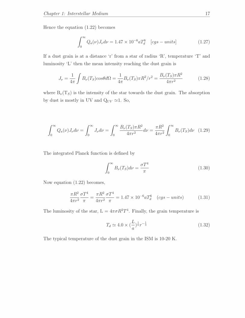
Hence the equation (1.22) becomes
∫ ∞
0
Qa(ν)Jνdν = 1.47 × 10⁻⁶aT 6d [cgs − units] (1.27)
If a dust grain is at a distance ‘r’ from a star of radius ‘R’, temperature ‘T’ and
luminosity ‘L’ then the mean intensity reaching the dust grain is
Jν =1
4π
∫
Bν(TS)cosθdΩ =1
4πBν(TS)πR2/r2 =
Bν(TS)πR2
4πr2(1.28)
where Bν(TS) is the intensity of the star towards the dust grain. The absorption
by dust is mostly in UV and QUV ≃1. So,
∫ ∞
0
Qa(ν)Jνdν =
∫ ∞
0
Jνdν =
∫ ∞
0
Bν(TS)πR2
4πr2dν =
πR2
4πr2
∫ ∞
0
Bν(TS)dν (1.29)
The integrated Planck function is defined by
∫ ∞
0
Bν(TS)dν =σT 4
π(1.30)
Now equation (1.22) becomes,
πR2
4πr2
σT 4
π=
πR2
4πr2
σT 4
π= 1.47 × 10⁻⁶aT 6
d (cgs − units) (1.31)
The luminosity of the star, L = 4πσR2T 4. Finally, the grain temperature is
Td ≃ 4.0 × (L
a)
16 r−
13 (1.32)
The typical temperature of the dust grain in the ISM is 10-20 K.

Chapter 1: Interstellar Medium 18
1.4.7 Polarization
Polarization of starlight arises when the light passes through the ISM containing
aligned elongated interstellar grains and depends on the degree of alignment with
the Galactic magnetic field. The light with electric vector parallel to the longer
axis of the aligned dust grain is more extinguished than the vector parallel to the
shorter axis and hence the polarization occurs. The wavelength dependence of
polarization (Pλ) is given by an empirical formula termed as ‘Serkowski’s Law’
(Serkowski et al. 1975):
Pλ = Pmax exp
−K
(
ln
(
λmax
λ
))2
(1.33)
where λmax (≈ 0.55 µm) is the wavelength of the maximum polarizarion Pλmax.
λmax value is typically in the range of 0.34 – 1µm with an average value of 0.55µm
(Sellgren et al. 1985) but varies for different lines of sight. The quantity, K de-
termines the width of the peak in the curve which was originally taken to be
1.15, but an improved fit (Wilking et al. 1982) gave the value of K = -0.10 +
1.86λmax. It is obvious from the Serkowski’s law that the polarization increases
with wavelength from near UV and reaches maximum in the optical and then falls
in the IR showing a little resemblance to the extinction law. In the IR wavelength
range this variation can be further approximated as Pλ ∝ λ−1.8 (Martin & Whit-
tet 1990a) with clear resemblance to extinction. Polarization is neither associated
with the bump (2175 A) nor FUV rise of extinction curve implying that small
grains are insufficient polarizers (may be spherical or less aligned)(Kim & Martin
1995). Polarization originates from the extinction of the light even though it shows
imperfect correlation with extinction. Strong polarization is seen in visible range
and its efficiency, Pmax/ Aλmax≤ 0.03 and this is the theoretical upper limit on
the polarization efficiency.
Apart from absorption, polarization is also observed inside molecular clouds in
emission at FIR. In emission, the polarization is largest in the direction of largest
absorption which is contrary to the optical polarization. Hildebrand et al. (1999)
have discussed the dependence of FIR polarization on optical depth and wave-
length in dense cloud cores and envelopes. Even though the grain alignments

Chapter 1: Interstellar Medium 19
are difficult in dense clouds as the dust grains are far from equilibrium with the
surrounding, the polarization is due to spinning of the grains due to anisotropic
starlight (Draine & Weingartner 1997).
1.4.8 Dust Scattering
Interstellar dust grains scatter electromagnetic radiation (both in ultraviolet and
visible) and the scattering efficiency depends on shapes, sizes, compositions and
distributions of the dust grains. Determination of intensity of the scattered radi-
ation requires knowledge of relative location of stars and grains. If the scattering
geometry is known, one can calculate the amount of radiation scattered in any
direction. However, the geometry is so complicated that optical parameters like
albedo and asymmetry parameter are used to delineate the scattering properties
of dust.
• Albedo (α) measures the fraction of the extincted light due to scattering,
α = Qc/Qe. Its value ranges from 0 (pure absorbers) to 1 (pure dielectric)
depending on the material of the dust and the observed wavelength.
• Asymmetry parameter (g) specifies the degree of scattering in a direction
and is defined as the mean value of the cosine of scattering angle weighted
with respect to scattering function.
g(θ) = 〈cosθ〉 =
∫ π
0S(θ)sinθcosθdθ
∫ π
0S(θ)sinθdθ
=2π
σsca
∫ π
0
S(θ)sinθcosθdθ (1.34)
Its value varies from -1 (completely backward scattering) to 1 (completely
forward scattering). Positive value of ‘g’ signifies scattering more towards
the forward direction and negative value means more toward the backward
direction where as g = 0 means scattering of light is isotropic.

Chapter 1: Interstellar Medium 20
• Scattering function S(θ) describes the angular distribution of scattered
light and it is related to scattering cross section (σsca) of dust grain by
σsca = 2π
∫ π
0
S(θ)sinθdθ (1.35)
An analytic and computationally convenient Henyey-Greenstein phase func-
tion (Henyey & Greenstein 1942) is used to measure the scattering radiation,
particularly in anisotropic multiple scattering approximations:
φ0(θ) =1
4π
1 − g2
(1 + g2 − 2gcosθ)3/2(1.36)
Scattering of light by dust grains is most efficient when the wavelength of light is
same as the size of the grains. Three main observational evidence of scattering of
light in the ISM are;
1. Diffuse Galactic light (DGL) – The scattering of ISRF by diffuse in-
terstellar dust grain constitutes diffuse Galactic light (DGL) which is strong
near the Galactic plane. The DGL is difficult to observe and analyze because
of its faintness and numerous sources of contamination. Its observation re-
quires careful correction for the contribution of faint stars, airglow and zo-
diacal light. The DGL is seen from the optical into the UV and its modeling
requires knowledge of the spectral dependence of the illuminating source over
the entire UV-optical wavelength range. The observed scattering properties
of interstellar dust are compared with the dust models to determine grain
properties such as albedo and scattering phase function.
2. Reflection nebulae – In reflection nebulae, light is scattered by a bright
star and is very conspicuous at optical and UV wavelengths when dust is
illuminated by the star. Study of scattering properties of dust in reflection
nebula is easier than the DGL as the spectral properties of the illuminating
star is better known than the ISRF. But reflection nebula suffers some dis-
advantages due to i) Unknown geometry of star and less known properties
of dust. ii) Patchiness of dust is a problem as determination of albedo and
scattering function is not easy for such distribution iii) The interpretation of

Chapter 1: Interstellar Medium 21
scattering angle is also a problem due to uncertain position of the star (star
may be in front, back or embedded).
3. Dust clouds – The dust clouds that are not close to a star are illuminated
by ISRF. The geometry of high Galactic dark clouds is better known than a
reflection nebula, for e.g., in optical wavelength band, the dark clouds bright-
ened by forward scattering grains where the illuminating source is behind
the cloud (FitzGerald et al. 1976). A lot of observations and modelings of
UV scattering by clouds at different latitude are done and few of them are;
observations of Cirrus cloud by Haikala et al. (1995), FUSE and Voyager
observations of Ophiuchus by Sujatha et al. (2005) and Coalsack by Sujatha
et al. (2007) and SPEAR/FIMS observations of the Taurus molecular cloud
by (Lee et al. 2006).
1.5 Heating Mechanisms in the ISM
There are several sources of energy for the interstellar gas viz., stars, X-rays,
cosmic-rays and transient events such as stellar wind, novae and super novae. The
ISM is heated by these energy sources which is then balanced by various cooling
processes giving rise to a thermal balance between them even though thermody-
namic equilibrium is rarely met in the ISM. In general, heating and cooling of the
ISM means the transfer of kinetic energy (KE) to and from atoms, molecules and
ions of interstellar gas. The heating process starts with photo-ionization where
an electron is removed from an interstellar species by an energetic photon. This
electron share its KE with other atoms, molecules and ions and heats the medium
by thermalization through elastic collision. Various heating mechanism of the ISM
are as follows:

Chapter 1: Interstellar Medium 22
1.5.1 Photoionization
Photoionization is the process of interaction of electromagnetic radiation with
atomic targets which results either removal or excitation of the electrons of the
atom. An energetic UV photon of frequency ν falls on an atom of ionization
potential ‘I’, yielding an electron ‘e’ with energy (hν-I) i.e.,
A + hν → A+ + e + (hν − I) (1.37)
This energy (hν-I) is carried by the electron which in turn heats up the gas by
colliding with atoms and ambient electrons of the ISM. In H II regions, photoion-
ization is a major heating process where ionization of H is dominant. Photons with
energy less than 13.6 eV also heats the gas by photoionization of heavy atoms, C,
Si, Fe and molecules.
1.5.2 Cosmic Rays
Cosmic rays (CRs) are quite efficient in heating the ISM. CRs can penetrate deep
into the molecular clouds and neutral ISM producing high temperatures. They
transfer energy to gas by ionization and excitation thus by producing free electrons
through Coulomb interactions. Low-energy CRs (E < 50 MeV) are more important
pertaining to heating mechanism because they are far more numerous than high-
energy CRs. The total ionization by CRs, ξCR, including secondary ionizations of
H and He is given by
nξCR = nξCR[1 + φH(E, xe) + φHe(E, xe)], (1.38)
Where the factors φH(E, xe) and φHe(E, xe) give the number of secondary ioniza-
tions of H and He produced per primary ionization (depends on electron energy)

Chapter 1: Interstellar Medium 23
and xe (ne/n) is the electron fraction (Wolfire et al. 1995). With a primary ion-
ization rate of 2×10⁻¹⁰ s−1, the total ionization rate of CRs is ξCR ≃ 3×10⁻¹⁰ s−1.
The heating rate is given by
nΓCR = nξCREh(E, xe), (1.39)
Eh(E,xe) is the average heat deposited per primary ionization. For low degrees of
ionization, Eh(E,xe) ≃ 7eV. Then the cosmic-ray heating rate is
nΓCR = 3 × 10⁻¹⁰n
[
ξCR
2 × 10⁻¹⁰
]
erg/cm3/s (1.40)
1.5.3 X-Rays
X-ray emission in ISM is produced mainly from the hot gas and is efficient in
heating warm, less dense atomic medium (Werner et al. 1970). X-rays remove
electrons from atoms and ions which can cause excitations or further ionizations
liberating other electrons like cosmic rays,
e + H(1s) → e + H(2p) → e + H(1s) + hν (1.41)
or
e + H(1s) → e + H+ + e (1.42)
The electrons liberated will go on ionizing the ISM until its energy is reduced to
less than 13.6 eV and there will be no excitation of H atoms when the energy is
less than 10.2 eV. The primary ionization rate of species ‘i’ due to soft X-ray is
given by
nξiXR = 4πn
∫
Jν
hνe−σνNHσi
νdν (1.43)
where the factor, e−σνNH is an absorbing layer of warm material of column density
N , Jν
hνis X-ray mean photon intensity, σν is X-ray photoionization cross-section

Chapter 1: Interstellar Medium 24
and σiν is that of the element ‘i’ (Wolfire et al. 1995). The heating rate is given by
nΓXR = 4πn∑
i
∫
Jν
hνe−σνNHσi
νEh(Ei, xe)dν cm−3s−1 erg/cm3/s (1.44)
where the summation extends over species which suffer primary ionization and
other symbols have usual meaning. Unlike cosmic rays, the X-ray ionization rate
and heating rate decreases with increasing depth of a cloud because of attenuation.
1.5.4 Heating by Photodissociation of Molecules
Photodissociation of H2 starts with absorption of FUV photon from ground elec-
tronic state to an excited electronic state followed by a radiative decay into the
vibrational continuum of the ground state in which nearly 10% of the molecule
dissociates. This radiative decay of the molecule gives rise to an emission of IR
photons or the molecule is de-excited through collisions if the density is high (n ≥
104), thereby heating the gas. The heating by this process is given by
nΓpd = 4 × 10⁻¹⁴n(H2)kpump erg/cm3/s (1.45)
The pump rate of molecular hydrogen is given by
kpump = 3.4 × 10⁻¹⁰β(τ)G0e(−2.6Av) s−1, (1.46)
where kpump is the pumping rate of UV photons that depends on β(τ), the reduc-
tion of the FUV pumping radiation due to self-shielding (optical depth τ ) by H2
and the exponential factor takes care of the dust absorption. G0 is the average
interstellar field (the Habing’s field). The heating efficiency of this process is given
by
ǫ(H2) ≃
(
Evib
hν
)
fH2 ≃ 0.17fH2 , (1.47)
where Evib is the vibrational energy converted into heat, hν is the energy of the
pumping FUV photon and fH2 is the fraction of the FUV photon pumping H2.

Chapter 1: Interstellar Medium 25
1.5.5 Chemical Heating
Molecular hydrogen (H2) is formed on the surface of dust grains when two H
atoms meet. This process is exothermic yielding an energy of 4.48 eV. A part of
this energy (4.2 eV) lifts the molecule to a rotational and vibrational excited state
and rest is converted into kinetic energy (0.2 eV) of the H2 molecule. This kinetic
energy as well as the energy released from de-excitation of the H2 by inelastic
collisions with other atoms and molecules heats the gas. The heating rate is given
by
ΓH2 = Rfn2xH(0.2 + 4.2η) eV/cm3, (1.48)
where Rf is the formation rate of H2 on grain surface, η is the fraction of the
excitation energy of H2 that is used for heating and xH is the fraction of gas
particle that are H atoms. Chemical heating is an efficient process in shocks and
dense photodissociation regions.
1.5.6 Photo-electric Heating
Small dust grains and large molecules such as PAH are efficient in photoelectric
heating which is an important mechanism in cold diffuse ISM. The UV radiation
emitted by hot stars can remove electrons from dust grains. A part of the photon
energy is used in removing the electron from dust grain and the remainder of the
photon’s energy heats the grain providing KE to the ejected electron that in turn
heats the gas. According to Mathis et al. (1977), size distribution of dust grains
n(a) ∝ a−3.5, and hence, the area distribution is, a2 × n(a) ∝ a−1.5 (a is the grain
radius). This shows that the smallest dust grains dominate photo-electric heating.
The photoelectric heating rate as derived by Bakes & Tielens (1994) is:
Γpe = 10−24ǫG0nH erg/cm3/s, (1.49)
where ǫ is fraction of the energy absorbed by grains that heats the gas,
ǫ =3 × 10⁻²
1 + 4.2 × 10⁻⁴G0T 0.5/ne
(1.50)

Chapter 1: Interstellar Medium 26
and G0 is the FUV flux normalized to Habing value (1.6× 10⁻³ erg/s/cm2) (Habing
1968).
1.5.7 Grain-Gas Heating
At relatively high densities, the collision of gas atoms and molecules with dust
grains leads to exchange of energy between them. The gas atoms colliding with
the dust grains can gain heat if the dust is warmer than the gas. This is an
important heating process in giant molecular clouds where the grains are heated
by the FIR radiations coming from outside. This radiation can penetrate deep
inside the cloud heating the gas that is at a lower temperature than the dust grain
(Falgarone & Puget 1985). The heating rate is given by
nΓg,d = nHndσd
(
8kT
πm
)1/2
2kα(Td − T ) erg/s/cm3, (1.51)
where nd is number density, σd =< πa2 > is geometrical cross section, Td is the
temperature of dust grain and T is the gas temperature (Td > T). α = T2−TTd−T
is
the accommodation coefficient, measures how well the gas atom accommodates to
the grain. T2 corresponds to an intermediate temperature between Td and T. In
ISM, σdnd = 1.5 × 10⁻²¹nH cm−1 and α = 0.35 (Burke & Hollenbach 1983). The
heating rate is given by
nΓgd ≃ 10−33n2HT 1/2(Td − T ) erg/s/cm3, (1.52)
1.5.8 Heating by Macroscopic Processes
Apart from the microscopic processes, there are several macroscopic processes such
as gravitational collapse of a cloud, Supernova explosions, stellar winds, expansion
of H II regions, Magneto-hydrodynamic waves created by supernova remnants play
major role in heating the gas although these processes are not delineated explicitly.
Gravitational collapse occurs during star formation as well as during the death of

Chapter 1: Interstellar Medium 27
a star. In this process, the material of a massive body is pulled inwards by its
own gravity generating a huge amount of energy which is dissipated as heat, thus
heating the gas of the ISM. Massive cataclysmic events like supernova explosion
and stellar winds pour a huge amount of mechanical energy into the ISM that goes
on heating the gas. Expansion of H II regions by champagne effect and collisionless
damping of interstellar magneto-hydrodynamic waves also heat up the gas upto
some extent.
1.6 Cooling Mechanisms in the ISM
Interstellar gases cool by emitting radiation. An atom, molecule or ion gets excited
gaining KE through collision with an energetic particle (electron, H, H+ etc.) and
gets excited. This excited specie undergoes radiative decay giving away its energy
as a photon which may escape the cloud thus by cooling the gas. Basically the
collisionally excited lines of metal play a critical role in the cooling mechanism.
The cooling process to be efficient there should be abundance of species to make the
collisions frequent and the gas should be optically thin, so that photons emitted
won’t be re-absorbed. This cooling process is efficient everywhere in the ISM
besides hot gas and regions deep within the molecular clouds. The cooling process
is given by
X + Y → X + Y ⋆ and Y ⋆ → Y + hν (1.53)
This hν amount of energy escapes out of the system and cools the gas. Various
cooling mechanism are described below.
1.6.1 Molecular Cooling
In molecular clouds, where temperature is less than few hundred Kelvin, the gas
is cooled by IR rotational lines. A molecule is excited by rotational or vibrational
transition and then returns to a lower energy state, emitting a photon which
can leave the region and cool the cloud. The molecules which contribute to the

Chapter 1: Interstellar Medium 28
cooling are CO, CH, OH and H2O by their electric dipole transition and H2 by its
quadrupole transition (Goldsmith & Langer 1978). The quadrupole transition of
H2 molecule occurs via ∆J=±2 transitions, the life time of which is very long (3
× 1010 sec). So, the population of this level, NJ increases, where
NJ ∝ (2J + 1)e(−EJ/kT ), (1.54)
Hence, radiation sheds out of this level slowly that is very unlikely to be re-
absorbed by H2. The cooling rate by H2 is given by
ΛH2 =∑
J≥2
n(H2, J)∆E(J → J − 2)A(J → J − 2) (1.55)
where the discrete value of energy EJ = BJ(J + 1), J=0,1,2... CO molecule
is an important coolant in denser clouds even though its abundance is low, ≈
10−5×N(H2). The cooling rate of CO which possesses a dipole moment transition
(∆J=±1) is given by
ΛCO =∑
J
n(CO, J)∆E(J → J − 1)A(J → J − 1) erg/s/cm3, (1.56)
1.6.2 Cooling by Resonance and Metastable lines
At higher temperature (T > 800 K), collisional excitation of n=2 level (metastable
level) of hydrogen will release a Lyα photon upon de-excitation which may escape
from the region cooling the cloud. Metastable transitions of C I, C II, O I, O II, Si
I, Si II, S I, S II, Fe I, and Fe II also contribute to the cooling (Wolfire et al. 1995). The
cooling by Lyα is given by
n2Λ(HI) = 7.3 × 10⁻¹⁹nen(HI)e−118400/T erg/s/cm3, (1.57)

Chapter 1: Interstellar Medium 29
1.6.3 Cooling by Dust
Interstellar dust grains are cooler than the gas in neutral diffuse medium and acts as
a coolant at high density (n ≥ 108 cm−3) shocks. The cooling rate per unit volume is
given by
Λgr = 1.2× 10⁻³¹n2
(
T
1000K
)1/2(100A
amin
)1/2
×[1− 0.8e(−75/T )](T −Tgr) erg/s/cm3,
(1.58)
where Tgr is the grain temperature, T is the gas temperature and amin is the minimum
radius of the grain.
1.6.4 Fine Structure Line Cooling
[C II] has a transition (2P1/2 → 2P3/2) at 158 µm with an energy corresponding to 92 K.
This is one of the important coolant of the gas clouds at low temperature. The cooling
rate per unit volume for C+ is
Λe,CII = 1.23 × 10⁻²⁷n2HdCe−92K/T (T/100)1/2 erg/s/cm3 (1.59)
The quantity dc is the depletion of carbon. C II can also be excited by collisions with
hydrogen atoms (Wolfire et al. 1995) and this gives
ΛH,CII = 7.9 × 10⁻²⁷n2HdCe−92K/T erg/s/cm3 (1.60)
where it is assumed that C and H nuclei are in C II and H I atoms.
1.6.5 Recombination
The radiative recombination of an electron with a proton or ionized species in an ionized
gas can cool the gas. The KE of the electron is removed from the thermal energy of the
gas, the energy loss of which is given by
Λreco = ne np k Te β(Te), (1.61)
Chapter 1: Interstellar Medium 30
where ne = electron density, np = proton density, Te = electron temperature, and β =
recombination coefficient.
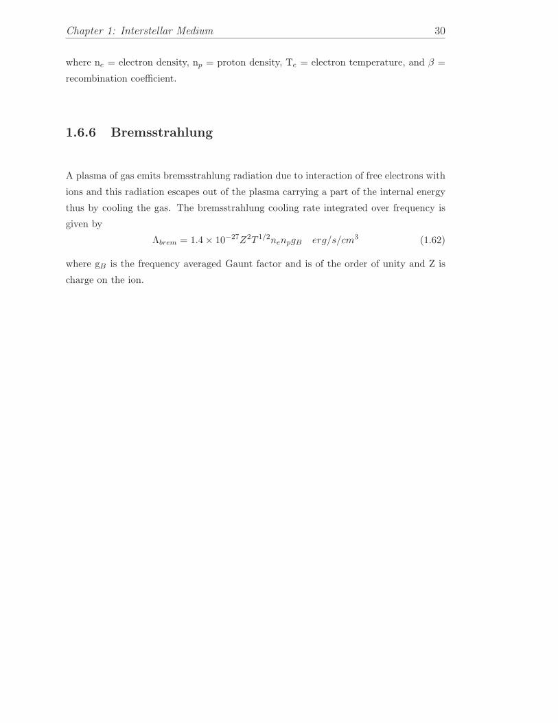
1.6.6 Bremsstrahlung
A plasma of gas emits bremsstrahlung radiation due to interaction of free electrons with
ions and this radiation escapes out of the plasma carrying a part of the internal energy
thus by cooling the gas. The bremsstrahlung cooling rate integrated over frequency is
given by
Λbrem = 1.4 × 10⁻²⁷Z2T 1/2nenpgB erg/s/cm3 (1.62)
where gB is the frequency averaged Gaunt factor and is of the order of unity and Z is
charge on the ion.

Chapter 2
Diffuse Background Radiation in
the Ultraviolet: Observations and
Data Reduction
2.1 Diffuse UV Background
Diffuse celestial backgrounds occur at all measurable wavelengths from radio wave to
gamma rays that carry a lot of information about the Universe. The origin of the
background emissions is related with wide variety of sources starting from the local ISM
to the farthest reach of the observable Universe. The diffuse background radiation at UV
occurs in the wavelength range of 900 – 3200 A. Over the past forty years, studies of the
diffuse UV backgrounds either by observations or model calculations suggest that the
possible sources of this could be Galactic and extragalactic. Although the extragalactic
sources have already been identified, the amount of extragalactic light coming to our
Galaxy is poorly constrained (Bowyer 1991).
The first observations of the diffuse UV radiation field were made by Hayakawa et al.
(1969) and Lillie & Witt (1969) from sounding rocket experiments who claimed that
diffuse UV light is due to star light scattered by dust. Subsequently, more observations
were made to measure the intensity of the diffuse UV background to investigate its
31

Chapter 2:Observation and Data Reduction 32
connection to the origin of Universe and Galactic evolution. There are excellent reviews
by Paresce & Jakobsen (1980); Bowyer (1991); Henry (1991); Murthy (2008) where
they have discussed the present status of observations and theories of the diffuse UV
background. Although several components contribute to the diffuse UV light, it is
dominated by radiation from hot stars scattered by interstellar dust grains, called Cosmic
UV background. A review by Leinert et al. (1998) on diffuse night sky brightness explains
all the components of diffuse radiation field over a wide range of wavelengths from far
UV to far IR in great detail.
2.2 Components of the Diffuse UV Radiation
• Dark Counts: Dark count is the instrumental background arising generally
through fast particles hitting the detector. It is inherent with the instrument
and difficult to remove. The typical count rate for low Earth orbit is of the order
of 5 counts cm−2 s−1. The count rate corresponding to this will depend on the
calibration and the field of view.
• Airglow: Airglow arises in the Earth’s atmosphere which is a strong function of
time of observation and height as it varies with changes in atmosphere and solar
activity (Meier 1991). It is produced by the collision of charged particles from
space, mainly from the Sun, with atoms and molecules in the upper atmosphere.
Airglow lines are the most deceptive sources that come into play while measuring
the diffuse UV radiation from satellites above the atmosphere. There are 20 major
airglow lines found above the earth’s atmosphere and the brightest among them
are the Lyman series lines(Lyα, Lyβ, Lyγ) seen upto the Lyman limit at 912
A where solar radiation is resonantly scattered by interplanetary hydrogen atoms
in the upper atmosphere at altitudes of greater than 1000 km. Other airglow lines
are less significant at night at 600 km or higher.
• Zodiacal light: Zodiacal light results from solar light scattered by interplanetary
dust grains. It mainly dominates in visible and IR, and less significant in the UV,
even its contribution to diffuse UV background drops to zero below 2000 A. It
is generally assumed that the colour of zodiacal light is similar to solar color
with moderate amount of reddening with respect to the Sun. Distribution of the
zodiacal light in the UV follows that in the visible.

Chapter 2:Observation and Data Reduction 33
• Unresolved stars: Unresolved stars influence the results of diffuse UV back-
ground as they come into the field of view of the instrument attempting to measure
the same. This problem may be solved by reducing the field of view of the instru-
ment and restricting the observations to high galactic latitudes where number of
hot stars are less and far apart. For fainter stars, theoretical stellar emission mod-
els and luminosity functions may be used with suitable stellar catalog to eradicate
the stellar contribution from the background measurements.
• Extragalactic light: In early 80s, it has been predicted that a measureble
amount of extragalactic diffuse background exists at all wavelengths with little
observational evidence. Expected sources of extragalactic background light in
UV are thought to be mainly from redshifted star light from unresolved galaxies,
integrated light from galaxies and QSOs, radiative decay of massive particles, col-
lisional excitation in dense IGM etc. and all these processes are delineated vividly
in reviews by Paresce & Jakobsen (1980); Paresce (1990). With the advent of UV
detectors with better sensitivity and resolution it has been proved that majority
of the UV background sources are within the Galaxy and a very small amount
being extragalactic, the possible upper limit of which is about 50 to 300 Photons
cm−2 s−1 sr−1 A−1 (Leinert et al. 1998).
2.3 Cosmic UV Background
Cosmic UV background is the component which originates beyond the solar system and
is mainly due to the scattering of star light by interstellar dust grains. Intensity of this
background depends on the distribution of hot stars, amount and distribution of dust,
optical depth, and the optical parameters of dust; albedo and phase function. Other
components of the cosmic background include atomic and molecular emission lines from
O VI (Shelton et al. 2007; Welsh et al. 2007; Dixon et al. 2001), C IV (Welsh et al.
2007), and molecular hydrogen (Martin et al. 1990b; Duley & Williams 1980). Based
upon observations made by FUSE (Murthy & Sahnow 2004) and Voyager (Murthy et
al. 1999), the diffuse radiation field over many different locations of the sky has been
mapped and it is argued that the diffuse FUV sky is patchy with regions of intense
emissions near bright stars (Figure 2.1).

Chapter 2:Observation and Data Reduction 34
Figure 2.1: Combination of the Voyager observations of Murthy et al. (1999)and the FUSE observations of Murthy & Sahnow (2004) into an Aitoff projectionof the diffuse FUV background with the Galactic center at the center of theimage and ±180 at the left and right edges, respectively. The area of each circleis proportional to the observed surface brightness with the large open circle atthe bottom right having a brightness of 2.9 × 10⁵ photons cm2 sr−1 s−1 A−1.
The background emission in UV and IR are important tracers of interstellar dust grains
as the scattering by dust in UV is complementary to that of the emission in IR. The
connection between the two wavelength bands can give good estimation of the dust
parameters. However, the value of the albedo and scattering phase function that deter-
mines the scattering properties of dust spans over a wide range of values when estimated
from the model calculations. Several works have attempted to study the relation of dif-
fuse UV with IR wavelength as well as the line of sight neutral hydrogen column density
for different celestial regions. Jakobsen et al. (1987); Perault et al. (1991); Haikala et
al. (1995); Sasseen & Deharveng (1996); Schiminovich et al. (2001) have showed that a
strong correlation exists between IR intensity at 100 µm as measured by IRAS and the
diffuse background intensity in the FUV wavelengths. Haikala et al. (1995) using the
FAUST data in FUV bands for a Galactic cirrus cloud, G251.2+73.3, near the north
Galactic pole have demonstrated that scattered UV light is correlated with the IRAS
100 µm surface brightness and the authors have also modelled the scatter light to esti-
mate the dust optical properties albedo (a=0.13±0.05 to 0.6±0.01) and scattering phase
function (g=0.0 to 0.9). Schiminovich et al. (2001) using NUVIEWS instrument mapped
the scattered UV light in four narrow UV bands which covers a one quarter of the sky

Chapter 2:Observation and Data Reduction 35
and found a good correlation of diffuse UV radiation with the IRAS 100 µm surface
brightness and a moderate albedo (a=0.45±0.05) and highly forward scattering phase
function parameter (g=0.77±0.1) over the same region. The existence of these proper-
ties thus provides strong observational support for the dust-scattered origin of most of
the FUV background.
A series of investigations were carried out to find the relation of UV background with
other Galactic parameters to provide an evidence to its origin. The most obvious param-
eter was the line of sight neutral hydrogen column density which showed a good correla-
tion between the two at high and intermediate Galactic latitudes (Paresce & Jakobsen
1980; Maucherat-Joubert et al. 1980b; Joubert et al. 1983; Jakobsen et al. 1984; Onaka
& Kodaira 1991; Hurwitz et al. 1991; Schiminovich et al. 2001) even though there is
no such strict relation between them. Existence of this correlation gives evidence of
Galactic component to the diffuse UV background due to scattering of starlight by high
latitude interstellar dust mixed with neutral hydrogen. Besides the positive correlation,
a positive offset of few hundred Photons cm−2 s−1 sr−1 A−1 is obtained which has been
thought to be due to contaminations or extragalactic component to the diffuse UV back-
ground (Hurwitz et al. 1991). The correlation of diffuse UV background with Galactic
latitude has also been tried (Weller 1983; Fix et al. 1989; Wright 1992; Sujatha et al.
2009, 2010; Murthy et al. 2010). Sujatha et al. (2009, 2010); Murthy et al. (2010) found
that the diffuse UV background follows a cosecant law with Galactic latitudes.
The satellites which are now producing exciting results on the diffuse UV radiation
field are Spectroscopy of Plasma Evolution from Astrophysical Radiation instruments
(SPEAR, also known as Far Ultraviolet Imaging Spectrograph or FIMS) and Galexy
Evolution Explorer (GALEX). The SPEAR/FIMS is a dual-channel FUV imaging spec-
trograph (S-band: 900-1150 A and L-band: 1350-1750 A) which covers 80% of the sky.
GALEX has observed 75% of the sky in two ultraviolet bands (FUV: 1350-1750A and
NUV: 1750-2850 A). A similar instrument to be launched by the Indian Space Research
Organization (ISRO) in end of 2012 is the Ultraviolet Imaging Telescope (UVIT) which
aims to observe the sky with a spatial resolution of 1.5 arcsecond in two UV channels
(FUV: 1200-1800 A and NUV: 1800-3000 A). Lee et al. (2006) measured diffuse FUV
continuum from the Taurus molecular cloud region with the SPEAR/FIMS imaging
spectrograph and observed an anticorrelation of this with molecular hydrogen fluores-
cent which indicates that molecular hudrogen is not a major contributor of diffuse UV
background. Similarly Seon et al. (2011) have presented far-ultraviolet (FUV: 1370-1720

Chapter 2:Observation and Data Reduction 36
A) continuum background over most of the sky, obtained with the SPEAR/FIMS in-
strument finding a good correlation of diffuse FUV continuum intensity with N(HI), 100
µm, and Hα intensities. Recently, some studies on diffuse UV observations (Sujatha et
al. 2009, 2010; Murthy et al. 2010) have done using data obtained with GALEX in both
FUV and NUV bands. Sujatha et al. (2009, 2010) have identified dust scattered diffuse
UV emissions for Draco and Sandage Nebulosity using Galex observations. Apart from
airglow and zodiacal emissions, they found an additional amount due to line emissions
from species such as CIV (1550 A) and Si II (1533 A) and H2 fluorescent. Similar stud-
ies have made by Murthy et al. (2010) where they have mapped diffuse UV background
which covers 75% of the sky except the Galactic plane and Magellanic Clouds. They
found that diffuse UV surface brightness correlates strongly with IR 100 µm emission
and follows cosecant law with Galactic latitude.
We used serendipitous observations made with the FUSE to report measurements of
the diffuse FUV (1000 - 1150 A) emission from the Magellanic Clouds (MCs). This
section comprises of the description on the FUSE and UIT along with the data reduction
technique to extract the diffuse FUV emission.
2.4 Far Ultraviolet Spectroscopic Explorer
The FUSE was launched in June, 1999 on a Delta II rocket into a nearly circular, low-
Earth orbit with an inclination of 25 to the equator and reached its termination in
October, 2007. The spacecraft and mission of FUSE have been described by Moos et
al. (2000) and Sahnow et al. (2000). The FUSE data is archived at the Multimission
Archive at the Space Telescope Science Institute (MAST). It was designed to observe sky
in the FUV spectral range from 905 to 1187 A upto a high resolving power of 20,000
(∆λ/λ). The primary purpose of FUSE was to explore the UV Universe with much
greater sensitivity and resolving power which was not achieved by any other instrument
then.
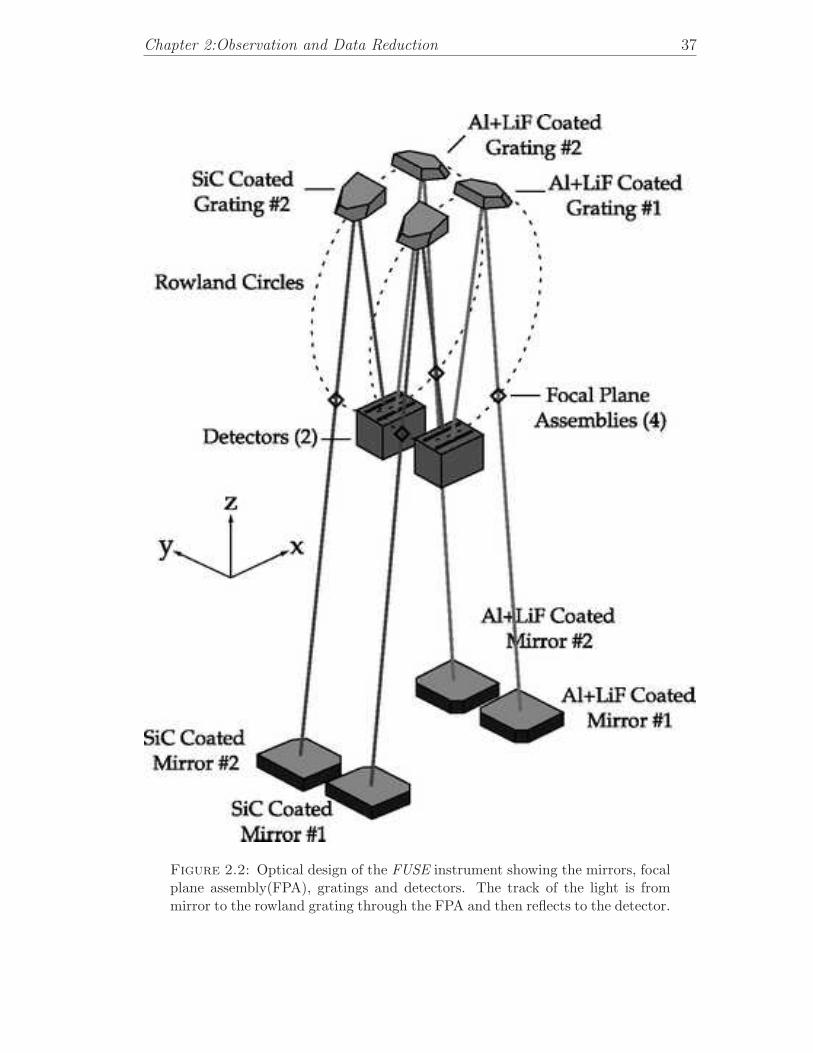
Chapter 2:Observation and Data Reduction 37
Figure 2.2: Optical design of the FUSE instrument showing the mirrors, focalplane assembly(FPA), gratings and detectors. The track of the light is frommirror to the rowland grating through the FPA and then reflects to the detector.
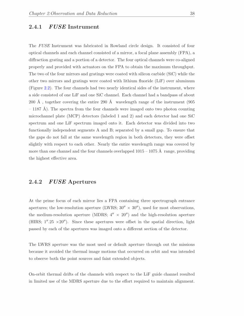
Chapter 2:Observation and Data Reduction 38
2.4.1 FUSE Instrument
The FUSE Instrument was fabricated in Rowland circle design. It consisted of four
optical channels and each channel consisted of a mirror, a focal plane assembly (FPA), a
diffraction grating and a portion of a detector. The four optical channels were co-aligned
properly and provided with actuators on the FPA to obtain the maximum throughput.
The two of the four mirrors and gratings were coated with silicon carbide (SiC) while the
other two mirrors and gratings were coated with lithium fluoride (LiF) over aluminum
(Figure 2.2). The four channels had two nearly identical sides of the instrument, where
a side consisted of one LiF and one SiC channel. Each channel had a bandpass of about
200 A , together covering the entire 290 A wavelength range of the instrument (905
– 1187 A). The spectra from the four channels were imaged onto two photon counting
microchannel plate (MCP) detectors (labeled 1 and 2) and each detector had one SiC
spectrum and one LiF spectrum imaged onto it. Each detector was divided into two
functionally independent segments A and B; separated by a small gap. To ensure that
the gaps do not fall at the same wavelength region in both detectors, they were offset
slightly with respect to each other. Nearly the entire wavelength range was covered by
more than one channel and the four channels overlapped 1015 – 1075 A range, providing
the highest effective area.
2.4.2 FUSE Apertures
At the prime focus of each mirror lies a FPA containing three spectrograph entrance
apertures; the low-resolution aperture (LWRS; 30′′ × 30′′), used for most observations,
the medium-resolution aperture (MDRS; 4′′ × 20′′) and the high-resolution aperture
(HIRS; 1′′.25 ×20′′). Since these apertures were offset in the spatial direction, light
passed by each of the apertures was imaged onto a different section of the detector.
The LWRS aperture was the most used or default aperture through out the missions
because it avoided the thermal image motions that occurred on orbit and was intended
to observe both the point sources and faint extended objects.
On-orbit thermal drifts of the channels with respect to the LiF guide channel resulted
in limited use of the MDRS aperture due to the effort required to maintain alignment.

Chapter 2:Observation and Data Reduction 39
It was intended to observe mostly the point sources.
The HIRS aperture was designed to maintain the highest resolution at the expense of
photometric accuracy. Its throughput was as high as 90% with minimum sky back-
ground. Because of the difficulties encountered with maintaining channel alignment
on-orbit, this aperture was used sparingly during the mission.
The science data obtained from a detector for an exposure yielded four data files for
each spectrum (LiF and SiC), labeled 1A, 1B, 2A, and 2B. All the three apertures of a
channel were open to the sky at a time producing three spectra, one from each of the
aperture.
2.4.3 Data Reduction Pipeline
The FUSE data is reduced by a data reduction software package, called CalFUSE. The
entire FUSE data set available at MAST has been reprocessed with CalFUSE v3.2,
the latest version of this software. The CalFUSE software takes care of the effect of
spacecraft motion, the instrumental effects, thermal drift correction, geometric distor-
tion correction, heliocentric velocity correction, dead time correction, wavelength cali-
bration, background subtraction, astigmatism correction, and screens the data for low
quality and unreliability. It is written in C programming language which consists of a
series of modules called by a shell script and each module corrects an effect during its
execution. The operation pipeline unified system (OPUS) is the data processing system
used in CalFUSE to combine spectra from each channel and exposures into a set of
observational level spectra. The data reduction and calibration process using CalFUSE
v3.2 is described by Dixon et al. (2007).
2.4.4 FUSE Observations
The primary purpose of the FUSE mission was to take high resolution spectra (λ/∆λ
≈ 20,000) of Galactic and extra-galactic sources. Although only the LWRS with its
relatively large field of view was useful for diffuse observations, there were many fields

Chapter 2:Observation and Data Reduction 40
in which the primary aperture was either the HIRS or the MDRS leaving the LWRS
aperture (separated from the other two apertures by 105′′ and 210′′, respectively) to
observe a nominally blank region of the sky. We downloaded the data from the MAST
archive at STScI and examined all for suitability for diffuse measurements. We rejected
all point source observations within the LWRS using the Object Class from the FUSE
archive. Then we were left with observations that were from two classes of targets: ob-
servations of point sources through either the MDRS or HIRS apertures; or calibrations
where the apertures were pointed at nominally blank areas of the sky in order to al-
low the spectrographs to thermalize before an instrumental realignment. We processed
all these observations using the latest version of the data pipeline software, CalFUSE
v3.2 (Dixon et al. 2007). Murthy & Sahnow (2004) have described the analysis of these
serendipitous background observations and we have followed their extraction of diffuse
surface brightnesses from the FUSE spectra.
The FUSE data consists of observations of both the day and the night part of the orbit.
Because of the faintness of the diffuse background, we have used only the night part
of the observations, thereby reducing the effect of all the airglow lines other than the
Lyman lines of atmospheric hydrogen. There are also additional lines like the weak O I
lines around 1040 A and N I lines at 1134 A but these lines don’t contribute significantly
to the continuum emission. Although the diffuse signal is visible in all the apertures,
we have used the data from LiF LWRS aperture because its throughput is much greater
than the others.
In each of the observations the diffuse signal in the LiF LWRS aperture clearly stands
out above the background. Still we found that the standard background subtraction
by CalFuse overestimates the instrumental background for the faint extended sources.
So, we have followed the procedure of Murthy & Sahnow (2004) to empirically estimate
the instrumental background, which is the counts between the regions on either side of
the aperture. We have set the limits to measure the diffuse flux and the instrumental
background from the detectors.
Figure 2.3 is an image of detector segment 1A of a FUSE observation. The LiF apertures
are imaged onto the top half and the SiC onto the bottom half of the image. Note that
the LiF 1A wavelength scale is increasing to right while the SiC 1A scale is increasing
to left. The enhancements due to the diffuse signal in the LiF LWRS aperture is clearly
seen. In the procedure of measuring the diffuse flux, we have treated FUSE as a broad

Chapter 2:Observation and Data Reduction 41
Figure 2.3: Image of the 1A detector segment of an observation. The LiFapertures are imaged onto the top half of the image and the SiC onto thebottom half with the terrestrial Lyβ line seen as the strongest line in each ofthe six apertures. Note that the defined bands (shown by the two large boxes)exclude the geocoronal Lyβ lines seen in the image (Murthy & Sahnow 2004).
band photometer and collapsed the spectra into two wavelength bands per detector,
excluding the terrestrial airglow lines (primarily Lyβ, 1026 A). The two boxes drawn
across the image show the wavelength limits of of the two bands (1A1: 988 – 1021 A and
1A2: 1035 – 1081 A) on either side of the Lyβ line. The bands have been collapsed into
corresponding effective wavelengths (1A1: λeff = 1003.93 A and 1A2: λeff = 1058 A)
to measure the integrated flux in each band.
The signal in the LiF LWRS aperture is plotted in the Figure (2.4) and we have then
fitted this profile with a Gaussian with uncertainties defined by the rms deviations
adjacent to the aperture and found 90% confidence limits on the level of the diffuse
background using the procedure of Lampton et al. (1976). The Gaussian was integrated
out to measure the diffuse emission in the band and the background was derived from
the strips off the spectrum and subtracted from the band flux. Similar procedure was
followed for all other detector segments and this resulted in seven wavelength bands with
effective wavelengths at 1004 A (1A1), 1058 A (1A2), 1117 A (1B1), 1157 A (1B2), 1159

Chapter 2:Observation and Data Reduction 42
Figure 2.4: Profile of LiF LWRS aperture used to measure the integrateddiffuse emission at band 1A2. The aperture limit is 510 – 620 and the back-ground limits are the rows 450 – 520 and 620 – 670. The fitted Gaussian is withconfidence limit of 90% which is shown by thick line (Murthy & Sahnow 2004).
A (2A1), 1112 A (2A2), 1056 A (2B1). The data from the 2B2 detector do not add any
value to the diffuse sky determination because of its much lower sensitivity. The bands
used for the extraction diffuse emission are listed in Table 2.1 and shown in Figure (2.5)
on top of a spectrum of the diffuse observation in N11, one of the brighter diffuse region
of the LMC. The integrated flux of each band is marked by a solid circle at its effective
wavelength.
Although we immediately rejected all observations which specifically observed a bright
star in the LWRS aperture, there were others where a star was coincidentally in the
aperture in the regions of high stellar density. These were identified and rejected through
their FWHM (Figure 2.4), which is less than 20 pixels for a point source but about 30
pixels for an aperture filling diffuse source.

Chapter 2:Observation and Data Reduction 43
Table 2.1: Bands Used for Extraction of Diffuse Emission
Number Bands Wavelength Range (A) Effective Wavelength (A)1 1A1 987.70 – 1020.77 1003.932 1A2 1034.84 – 1081.37 1058.113 1B1 1100.28 – 1133.69 1117.004 1B2 1133.70 – 1180.07 1156.885 2A1 1175.32 – 1141.97 1158.656 2A2 1128.57 – 1095.03 1111.807 2B1 1069.11 – 1035.41 1056.00
Figure 2.5: Spectrum of N11 (PGMW-3053) showing the seven wavelengthbands that have been integrated to obtain the FUV diffuse emission. The wave-length range is marked by horizontal bars at the bottom of the spectrum andthe integrated fluxes of each band by solid circle at their effective wavelengths.

Chapter 2:Observation and Data Reduction 44
2.5 Ultraviolet Imaging Telescope (UIT)
2.5.1 UIT Instrument
The Ultraviolet Imaging Telescope (UIT) flew onboard the Space Shuttle Columbia as
part of the Astro payload in December 1990 and again in March 1995. This payload
consisted of three co-mounted ultraviolet instruments: the UIT, the Hopkins Ultra-
violet Telescope (HUT), and the Wisconsin Ultraviolet Photo-Polarimeter Experiment
(WUPPE). The UIT is an f/9 Ritchey-Chretien telescope with 38cm aperture. It was
equipped for UV (1200 – 3300 A) images of astronomical objects with a field of view
of 40′ and resolution of about 3′′. It contained two detector systems: one in the far
UV (‘B’ filters) and one in the near UV (‘A’ filters). Images were recorded on 70 mm
photographic film. The details of the UIT instrumentation, pipeline, data reduction and
calibration are explained by Stecher et al. (1997). The UIT data from both the Astro
missions are available at MAST.
2.5.2 UIT Observations of the MCs
We have used the calibrated and geometrically corrected images of the UIT (2048 x 2048)
from the MAST that overlap with some of the FUSE observations and are analyzed by
Parker et al. (1998) for the LMC and by Cornett et al. (1997) for the SMC. All these
images are observed with FUV B-Camera filters: B1 (λeff = 1521 A and ∆λ = 354 A)
and B5 (λeff = 1615A and ∆λ = 225 A) of the UIT. But the FUSE LWRS aperture
size is 30′′ x 30′′ which is much larger than the 1′′.13 pixels of the UIT, therefore, we
have integrated the 37′ UIT images over 27 x 27 pixel box to measure the UIT diffuse
flux which is then compared with the diffuse fluxes of the FUSE bands.
2.5.3 Conversion of UIT flux to Photon units
In order to compare the FUSE observations with the UIT, the fluxes observed by both the
instruments should have the same physical units. The UIT fluxes have been converted

Chapter 2:Observation and Data Reduction 45
from erg cm−2 s−1 A−1 to photons cm−2 s−1 sr−1 A−1 (Fλ/hν). The effective wavelength
of the UIT B1 and B5 filters are 1521 A and 1615 Arespectively. For B1 filter: F erg
cm−2 s−1 A−1 = 1521×F/(6.62×3×10−9) photons cm−2 s−1 A−1. 1′′ equivalent solid
angle is Ω = (π/180×1/3600)×(π/180×1/3600). The UIT images are with 1′′.13 pixels
and the solid angle of 1′′.13 is Ω = (π/180×1.13/3600)× (π/180×1.13/3600) steredian.
For B1 filter: F erg cm−2 s−1 A−1 = 1521×F/(6.62×3×10−9/Ω) photons cm−2 s−1 sr−1
A−1 and same procedure is followed for B5 filter.
2.6 Stellar Radiation Field Model
We have used Stellar Radiation Field Model of Sujatha et al. (2004), that is one of the
tools in Tauvex web page (http://tauvex.iiap.res.in/htmls/tools/fluxcalc) to translate
flux of a star from the UIT band to the FUSE bands. This calculation is based on
Kurucz models (Kurucz 1992) and scaled down to visual magnitude which requires
three parameters (Visual magnitude, extinction and spectral type) as input to obtain
the spectrum of a star in a wavelength range of 900 – 10000 A. The theory involved in
this model is as follows:
If I0 is the intensity at the surface of a star, then the reduced intensity of the beam of
the star after traveling through a dust cloud of optical depth τ is,
I = I0e−τ (2.1)
but I = 4πd2f and I0 = 4πr2f0 (2.2)
So, 4πd2f = 4πr2f0e−τ (2.3)
where f = flux of a star at a distance ‘d’ and r = radius of the star.
f = (r/d)2f0e−τ (2.4)
If f0 = Kurucz flux at 5500 A= K, then
f = (r/d)2Ke−τ = ΓKe−τ (2.5)

Chapter 2:Observation and Data Reduction 46
where Γ = Scaling factor. From the flux magnitude relation, we know,
m1 − m2 = −2.5log(f1/f2) (2.6)
The most popular standard and reference for all broad band photometry is the star Vega
(spectral type A), whose apparent magnitude is zero. Substituting the flux density in a
given filter of Vega for f2 and putting m2 =mvega = 0, the zero magnitude flux (3.64e−9
erg cm−2sec−1A−1) and m1 = V, we get
f = 3.64e−9 × 10−V/2.5 (2.7)
Hence finally,
ΓK(5500A)e−τ = 3.64 × 10−9 × 10−V/2.5 (2.8)
where τ = AV /1.0863 = E(B V).RV /1.0863. The extinction and visual magnitude are
the unknown parameters which is to be supplied. Assuming these and using the Kurucz
model flux (K) of appropriate spectral type, the scale factor, Γ is estimated and then
the modeled spectrum of a star is obtained.
2.7 Calculation of Errors in Diffuse Fraction
FUV diffuse fraction = diffuse flux/(diffuse flux + stellar flux)
DF = Diffuse FUSE flux
DU = Diffuse UIT flux
R = slope of the FUSE- UIT correlation = FUSE/UIT
SF = Stellar flux
df = FUSE diffuse fraction
DF = R × DU
erDF = (erR/R + erDU/DU) × DF
where erR is the error in R calculated from the least square fitting of FUSE and UIT
correlation, erDU is error in DU = 10% obtained (Parker et al. 1998).
df = DF/(DF + SF)
dfmax = (DF + erDF)/[(DF - erDF) + (SF - erSF)]
dfmin = (DF - erDF)/[(DF + erDF) + (SF + erSF)]
Maximum error in df = dfmax - df
Minimum error in df = df - dfmin

Chapter 3
Far Ultraviolet Diffuse Emission
from the Large Magellanic Cloud
3.1 Introduction
The LMC and the SMC are two dwarf irregular galaxies visible in the southern hemi-
sphere known as Magellanic Clouds (MCs). The irregular structure of MCs may be due
to the tidal interaction between them and with the MW. The MCs were discovered by
Ferdinand Magellan on his voyage in 1519. Both the galaxies are orbiting the MW and
thus, are members of the local group of galaxies.
A long tail of gas extending from the MCs is called the Magellanic Stream. This is
only visible in radio wavelength and its origin is believed to be due to the gravitational
interaction between the MW and the MCs. There is a bridge of neutral hydrogen gas
connecting the SMC and the LMC, which is evidence of tidal interaction between both
the galaxies. Streamers of gas that is being stripped from the MCs and falling into the
MW is called the Leading Arm (Figure 3.1).
The LMC spans 8 across the sky with the center RA: 05h 23m 34.5s (80.89) and
Dec: -69 45′ 22′′ (-69.76) (gl = 280.46 and gb = -32.88). It was considered the
nearest galaxy to the MW (50 kpc; Feast 1999) until the discovery of the Sagittarius
47

Chapter 3: The LMC 48
Figure 3.1: CSIRO’s Parkes radio telescope image of the MCs.
Dwarf Elliptical Galaxy and Canis Major Dwarf Galaxy. It is a treasure house of variety
of astronomical objects with rich in gas and dust, and home to the supernova 1987A,
60 globular clusters, 400 planetary nebulae, 700 open clusters, 32 known supernova
remnants, and more than 30 billion stars. Two morphologically analogous and immense
star forming regions in the LMC are the 30 Doradus , and the N11 region, present in
diametrically opposite end of the prominent central Bar. 30 Doradus, the largest H II
region in the LMC is the largest star forming region in the local group of galaxies. The
energy for this nebula comes from a central star cluster R136 (comprising of O type
stars) which makes the nebula visible. N11 is the second largest H II region in the
LMC after 30 Doradus, and is home to several associations of massive stars; LH9, LH10,
LH13, and LH14 (Lucke & Hodge 1970). The LMC has a mass of 9 ×10⁹M⊙ (van der

Chapter 3: The LMC 49
Marel et al. 2002), and a star formation rate of 0.1 M⊙/yr (Whitney et al. 2008).
The LMC provides a very different view of the ISM than is possible either from obser-
vations of the MW or of other, more distant galaxies. At a distance of 50 kpc (Feast
1999), it is far enough that we can get an overview of processes in the entire galaxy but
close enough that we can distinguish between the different sources. It is also oriented
almost face-on (viewing angle of 35; van der Marel & Cioni 2001) which allows study
of the ISM emissions without any confusion along the line of sight. The LMC has lower
metallicity (Z ≈ 0.3 – 0.5 Z⊙; Westerlund 1997) consistent with the reduced dust to gas
ratio(EB−V
NH≃ 4.5 × 10⁻²³ mag cm2/H; 26% less than the MW). The ratio, AV
NHin-
creases from the outskirts of the LMC towards the 30 Doradus star-forming region which
could be either due to a systematic increase of the dust abundance or the presence of
an additional gas component not traced by H I. The extinction curve of the LMC with
a weaker bump at 2175 A and a steeper FUV rise is different from the MW (Clayton &
Martin 1985; Misselt et al. 1999; Gordon et al. 2003) although it is similar in the visible
and near-IR (Clayton & Martin 1985).
Since its discovery, LMC has been center of many surveys at different wavelengths. The
distribution of H I has been mapped at low resolution by Luks & Rohlfs (1992) and
at high resolution by Kim et al. (1998) showing that N(H I) in the LMC is chaotic
with hundreds of clumps, shells, filaments. The ionized-gas content has been imaged in
Hα photographs (Meaburn 1980; Kennicutt & Hodge 1986) and in the radio continuum
(Haynes et al. 1991; Dickel et al. 2005) and both shows a variety of interstellar shells,
ranging more than a few hundred parsecs across. The stellar contents of the LMC
have been widely studied by photometry of stars from the near-IR to the UV bands
(Parker et al. 1998; Ita et al. 2004; Zaritsky et al. 2004; Blum et al. 2006; Kato et al.
2007). Soft X-ray images of the LMC have been obtained by ROSAT (Snowden & Petre
1994), revealing a variety of discrete sources like supernova remnants and X-ray binaries.
CO surveys of molecular gas (Israel et al. 1986; Cohen et al. 1988; Fukui et al. 1999,
2008) depicts individual molecular structures in the LMC. Howk et al. (2002a) surveyed
the distribution and kinematics of highly ionized gas O VI towards 12 early type stars
and Lehner & Howk (2007) analyzed the absorption of O VI, C IV, Si IV and N V
ions towards four early type stars in the LMC which provide crucial details about the
environments that may be probed through the study of these ions.
The recent high angular resolution IR studies by Spitzer Surveying the Agents of Galaxy

Chapter 3: The LMC 50
Evolution (SAGE) legacy survey (Meixner et al. 2006; Bernard et al. 2008) and low
angular resolution surveys by IRAS and DIRBE (Sauvage et al. 1990; Sakon et al.
2006) have allowed the observer to resolve separation of the diffuse emission from the
point sources. This is an important pre-requisite for understanding the physics of dust
emission, since the emission depends strongly on the intensity of the ISRF and on the
relative distribution of dust and stars. The most comprehensive survey of dust and gas
in the LMC has come from Bernard et al. (2008) and Paradis et al. (2009) using a variety
of sources including new observations with the Spitzer Space Telescope (Meixner et al.
2006). Bernard et al. (2008) found that there was a modification of the dust population
in the LMC as compared with the MW, perhaps through the erosion of large grains in
the ISM.
Different regions in the LMC have significantly varying stellar population,dust and gas
distribution. The 30 Doradus, N11, N4, N70 regions are rich in OB associations and
young stars while the LMC bar region is mostly populated by old stars. The LMC
bar region is rich in gas and molecules incorporated with fresh dust out flowing from
AGB stars where as the 30 Doradus and the regions around it have a more evolved
and relatively bigger size dust population (Paradis et al. 2009). The results of Paradis
et al. (2009) show that each dust component could have different origin and evolution
in the ISM; they predicted that VSGs could have originated from shattering of BGs
where as PAHs could have been injected into the ISM during the mass loss from old
stars. The relative abundance of PAHs is more in bar and molecular cloud regions
where as the VSGs abundance is more over the 30 Doradus region. The distinct spatial
distribution of the PAHs and VSGs agrees the trend that PAHs abundance follows
the more quiescent environments while the VSGs abundance follows the star formation
activity. It is also evidenced that these two dust components could have different origin
or different processing in the ISM of the LMC (Paradis et al. 2009).
3.2 Ultraviolet Observations of the LMC
The LMC is an ideal location to study the connection between dust and diffuse UV light.
The first imaging observations of the LMC in the UV were by Page & Carruthers (1981)
using the S201 FUV camera during the Apollo 16 mission followed by Smith et al. (1987)
from a rocket experiment and Parker et al. (1998) from the UIT on board the Space
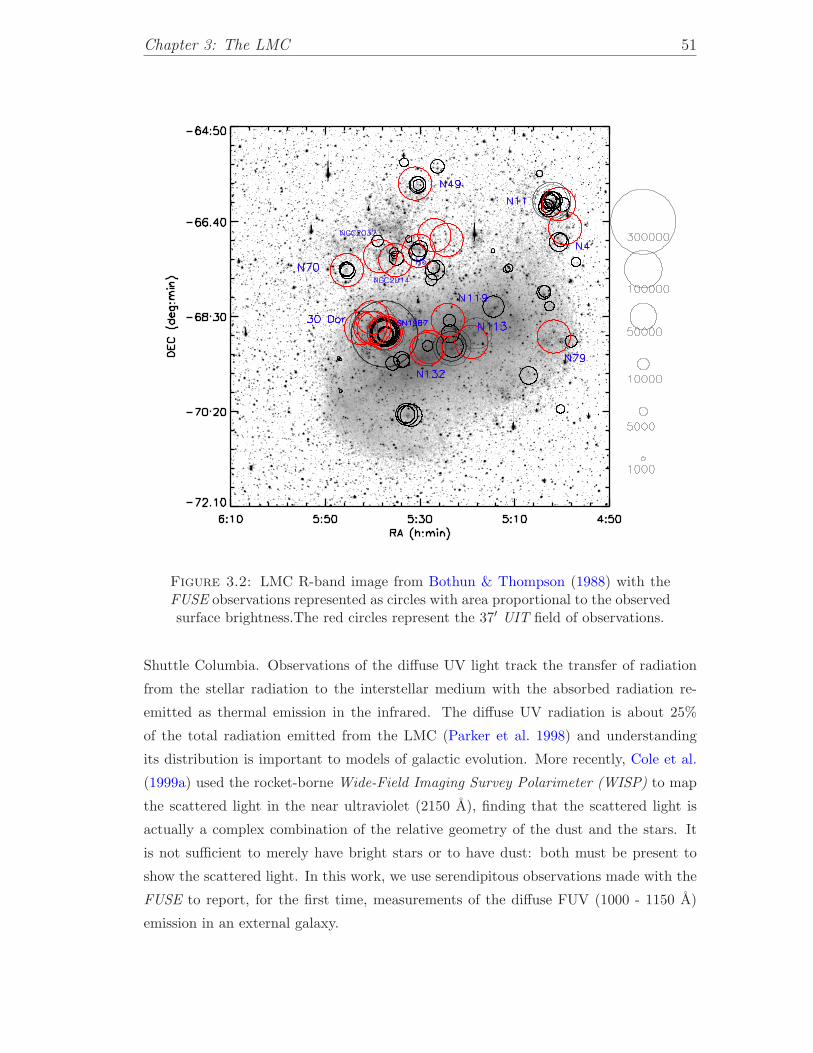
Chapter 3: The LMC 51
Figure 3.2: LMC R-band image from Bothun & Thompson (1988) with theFUSE observations represented as circles with area proportional to the observedsurface brightness.The red circles represent the 37′ UIT field of observations.
Shuttle Columbia. Observations of the diffuse UV light track the transfer of radiation
from the stellar radiation to the interstellar medium with the absorbed radiation re-
emitted as thermal emission in the infrared. The diffuse UV radiation is about 25%
of the total radiation emitted from the LMC (Parker et al. 1998) and understanding
its distribution is important to models of galactic evolution. More recently, Cole et al.
(1999a) used the rocket-borne Wide-Field Imaging Survey Polarimeter (WISP) to map
the scattered light in the near ultraviolet (2150 A), finding that the scattered light is
actually a complex combination of the relative geometry of the dust and the stars. It
is not sufficient to merely have bright stars or to have dust: both must be present to
show the scattered light. In this work, we use serendipitous observations made with the
FUSE to report, for the first time, measurements of the diffuse FUV (1000 - 1150 A)
emission in an external galaxy.

Chapter 3: The LMC 52
3.3 FUV Diffuse Emissions in the LMC
There were more than 600 FUSE observations within 5 of the LMC. We downloaded
them and first rejected all point source observations within the LWRS using the Object
Class from the FUSE archive. This gave a total of 172 observations. Then we were left
with 81 observations of the diffuse radiation in different parts of the LMC after checking
the FWHM of the LWRS aperture for the diffuse sources. The details of the diffuse
observations are given on Table 3.2. The intensities of FUV diffuse radiation range from
around 103 photons cm−2 s−1 sr−1 A−1 to as high as 3 × 10⁵ photons cm−2 s−1 sr−1
A−1 near 30 Doradus. Although we have listed all the diffuse values for completeness,
we note that the effective lower limit for the detection of diffuse radiation with FUSE
is about 2000 photons cm−2 s−1 sr−1 A−1 (Murthy & Sahnow 2004). The LMC is at
a high Galactic latitude where the contribution from the Galactic diffuse radiation will
be relatively small and we have estimated it to be on the order of 500 photons cm−2
s−1 sr−1 A−1, based on nearby Voyager observations by Murthy et al. (1999). We have
plotted the diffuse flux in one of the FUSE bands (1B1 at 1117 A) as circles with areas
proportional to the observed surface brightness in Figure 3.2. There is an excellent
correlation between the diffuse FUV flux observed in 1B1 and each of the other FUSE
bands with linear correlation coefficients of better than 0.9 in each case and a similar
plot would be obtained for any of the other bands. One of the correlation plots between
the FUSE bands is shown in Figure 3.3. The correlation co-efficient of the plot is 0.99
and the best fit line is with slope 0.62 and an offset of -32 photons cm−2 s−1 sr−1 A−1.
Cole et al. (1999a) found that their diffuse light (2150 A) was dominated by the N11
complex in the northwest LMC with a surface brightness of 104 photons cm−2 s−1 sr−1
A−1, which they identified as a giant reflection nebula. Although, certainly bright in our
FUSE observations, by far the brightest of our observed regions is around 30 Doradus
(the Tarantula Nebula), which was not observed by WISP. As mentioned above, the
FUSE targets have been selected for their proximity to bright stars and as a result,
almost all of our observed diffuse regions are also bright. The FUV diffuse emission in
the LMC is predominantly due to the scattering of the star light from the OB associations
and shows a large variation in a small angular scale, particularly in 30 Doradus and N11
regions (Figure 3.2). These regions are rich in hot OB stars of UV magnitudes less than
10 (Parker et al. 1998) and show significant variation in stellar density in a small angular
scale.

Chapter 3: The LMC 53
Figure 3.3: The correlation between 1A1 and 1B1 band of FUSE.
3.4 FUSE – UIT Correlation
We have extensively used the UIT data to estimate the fractional contribution of FUV
diffuse radiation in the LMC. Wide field far ultraviolet images of the regions of nebulosity
cataloged by Davies et al. (1976)(DEM) have been obtained by the UIT. Of the H II
regions in the catalog of DEM, the UIT covers 102 regions in the LMC and 74 regions
in the SMC. Out of them 16 fields from the LMC have been analyzed by Parker et al.
(1998) and we have used their images for the calculation of diffuse UV emission. Parker
et al. (1998) have measured the total integrated aperture flux as well as stellar flux
within each of the regions and they have also provided a catalog of FUV magnitudes
derived from point spread function photometry for 37,333 stars of these regions.
Of the 81 FUSE locations, 43 overlapped with 10 UIT field of observations in the LMC
for which we measured the UIT flux. The UIT fluxes were then converted from erg cm−2
s−1 A−1 to photons cm−2 s−1 sr−1 A−1. We found a strong correlation between UIT
flux and diffuse flux in 1B1 band (Figure 3.4). Three points in the 30 Doradus region

Chapter 3: The LMC 54
Figure 3.4: Correlation between the FUSE (1B1) and the UIT surface bright-ness is shown. The correlation coefficient is 0.78 but rises to 0.92 if four points(three of the 30 Doradus and one of the N11 points) are removed. The bestfit is the line with slope 0.28 and an offset of -6730 photons cm−2 s−1 sr−1
A−1. Similar plots are obtained for the other six FUSE bands. Errors in theobservations are small (relative to Y-axis scale) to be visible and are not shown.
have a relatively higher FUSE flux because the radiation field is dominated by O stars
in the nebula whereas one observation in N11 had a relatively higher UIT flux because
the stellar spectrum is much flatter than in other regions. Similar correlation plots of
UIT diffuse flux with other FUSE bands were obtained to determine the best fit slope
i.e., FUSE/UIT ratio.
3.4.1 Calculation of Diffuse Fraction
Rather than deal with absolute values, a useful comparison is to find the fractional
amount of diffuse radiation in the field defined as diffuse radiation over total radiation
(diffuse + stellar) in each of the UIT regions. We obtained the FUV magnitudes of all

Chapter 3: The LMC 55
Table 3.1: Calculation of Far Ultraviolet Diffuse Fraction (DF) for the FUSE1B1 (1117 A) band.
UIT Total flux DF(UIT) FUSEUIT
Total flux Stellar flux DFField UIT FUSE FUSE FUSE
30 Doradus 1.50e-10 0.50 0.26 1.91e-11 2.31e-10 0.077SN1987 3.00e-10 0.28 0.26 2.14e-11 5.63e-10 0.037N51 1.40e-10 0.55 0.26 1.97e-11 1.89e-10 0.094NGC-2014 1.50e-10 0.58 0.26 2.22e-11 1.12e-10 0.166N113 1.30e-10 0.43 0.26 1.43e-11 2.31e-10 0.058N119 1.90e-10 0.41 0.26 1.99e-11 1.73e-10 0.103N132 1.20e-10 0.61 0.26 1.87e-11 1.02e-10 0.155N4 1.00e-10 0.69 0.26 1.76e-11 8.64e-10 0.169N11 2.10e-10 0.43 0.26 2.31e-11 2.74e-10 0.078N70 6.30e-11 0.84 0.26 1.35e-11 2.17e-11 0.384
the stars contained in each of the UIT field from the catalog of Parker et al. (1998).
The magnitude was converted to flux using Hayes & Latham (1975) formula: m(λ) =
-2.5logF(λ) - 21.1. Then the flux of a star of given spectral type was translated from
UIT bands to FUSE bands using Stellar Radiation Field Model of Sujatha et al. (2004)
that is based on Kurucz models (Kurucz 1992) and the fluxes of all the stars in a given
field were summed to obtain the total stellar flux in FUSE bands. The total integrated
aperture flux and the fraction of the total flux in diffuse radiation in each field in the
UIT band is estimated by Parker et al. (1998). With the observed FUSE/UIT diffuse
ratio, we could then calculate the total amount of diffuse radiation at each of the FUSE
bands which is the FUSE/UIT times the total UIT diffuse flux of that region and thus,
the fraction of total light emitted as diffuse emission i.e., diffuse/(stellar + diffuse). We
have not considered extinction as it will affect both the stellar and diffuse flux equally
and so will cancel out. Table 3.1 shows the calculation of diffuse fraction for the UIT
fields at 1B1 band of the FUSE. These fractions range from 5% to 20% of the total at
1100 A, with a high of 45% in the superbubble N70, with an observed error of 12% –
17%. The comparable estimate for the MW is 10% (Parravano et al. 2003). The error
bars in the diffuse fraction were empirically calculated by taking the extremes of the
observed fluxes.

Chapter 3: The LMC 56
Figure 3.5: Variation of diffuse fraction against wavelength for different UITregions of the LMC. Also plotted are the albedo (dashed line) and cross-section(dot-dashed line divided by 7.6 × 10⁻²²) from model calculations by Weingart-ner & Draine (2001). The seven observed FUSE bands are shown at four wave-lengths (1004, 1057, 1114.5 and 1158 A), where the intensities at 1057, 1114.5and 1158 A are average of the 1A2 & 2B1 bands, 1B1 & 2A2 bands, and 1B2& 2A1 bands respectively. The error bars were empirically calculated by takingthe extremes of the observed fluxes which range from 12% – 17% of the data.
3.5 Discussion
Although some part of the variation of diffuse fraction in different regions of the LMC
may be due to the dust distribution, it is likely that much of the stellar radiation is
non-local, as noted by Cole et al. (1999a) i.e., the diffuse light may come from stars
far away from the observed area. In our Galaxy, this is seen as scattering of galactic
plane star light by high latitude dust clouds (Jura 1980); in the LMC, light from the
OB associations will be scattered by distant dust. The shape of the diffuse fraction is
essentially the same in all the 10 regions rising by a factor of about 5 from 1000 to 1500
A. The lower value of diffuse fraction at shorter wavelength implies that most of the
heating of the interstellar dust comes in the FUV which is well proved by Law et al.

Chapter 3: The LMC 57
(2011) for star forming galaxies using Spitzer data and dusty radiative transfer model.
The variation of diffuse fraction with wavelength is consistent with variation of albedo
(dashed line) and cross-section (dot-dashed line) of the grains in the FUV (Figure 3.5)
saying that less light is scattered in FUV.
Cole et al. (1999b) have attempted to model the distribution of diffuse light in the WISP
data by scattering the light of OB associations in the LMC from a dust distribution which
decays exponentially with radius and with a hyperbolic secant with distance from the
plane. They found that although their models did match the overall morphology of the
observations, it was difficult to constrain the parameters because of the uncertainty in
many of the physical properties of the ISM in the LMC, particularly in its clumping.
Nevertheless they did find that 30 Doradus dominated the diffuse emission in the eastern
LMC, a conclusion borne out by our FUSE observations in the FUV.
3.6 Conclusions
We have obtained the first FUV (1000 – 1150 A) spectra of the diffuse radiation in an
external galaxy using serendipitous FUSE observations of targets in the LMC. Most of
these observations are near OB associations and the diffuse emission is bright, ranging
from 5% to 20% of the total flux in the region. This fraction is much less than the
corresponding fraction emitted at 1500 A suggesting that the largest part of the heating
of the interstellar dust occurs in the FUV.

Chapter
3:T
heLM
C58
Table 3.2: Details of the FUSE observations in the LMC.
Target Name RA Dec LiF 1A1 LiF 1A2 LiF 1B1 LiF 1B2 LiF 2A1 LiF 2A2 LiF 2B1
SK-68.75 80.91 -68.15 (14.46 ± 8.52)E+03 (4.94 ± 1.41)E+03 (9.12 ± 3.79)E+03 (8.11 ± 2.98)E+03 (7.02 ± 2.31)E+03 (4.87 ± 1.20)E+03 (4.55 ± 1.95)E+03
SK-67.106 81.65 -67.55 (18.12 ± 1.73)E+03 (20.55 ± 1.05)E+03 (21.41 ± 1.71)E+03 (25.25 ± 1.76)E+03 (23.17 ± 1.50)E+03 (22.83 ± 1.51)E+03 (20.15 ± 1.72)E+03
SK-67.107 81.67 -67.55 (14.10 ± 1.47)E+03 (168.88 ± 8.97)E+02 (18.59 ± 1.57)E+03 (19.56 ± 1.85)E+03 (19.50 ± 1.35)E+03 (17.36 ± 1.06)E+03 (19.80 ± 1.48)E+03
PGMW-3053 74.30 -66.39 (76.34 ± 1.46)E+03 (995.20 ± 8.89)E+02 (104.27 ± 1.67)E+03 (127.56 ± 1.91)E+03 (129.17 ± 1.34)E+03 (115.69 ± 1.17)E+03 (88.34 ± 1.20)E+03
PGMW-3070 74.31 -66.39 (64.55 ± 1.42)E+03 (798.40 ± 8.64)E+02 (78.71 ± 1.66)E+03 (86.39 ± 2.00)E+03 (107.84 ± 1.72)E+03 (101.11 ± 1.57)E+03 (87.35 ± 1.56)E+03
PGMW-3168 74.36 -66.38 (19.53 ± 1.09)E+03 (247.82 ± 6.65)E+02 (26.67 ± 1.13)E+03 (28.34 ± 1.04)E+03 (35.18 ± 1.17)E+03 (33.51 ± 1.27)E+03 (26.56 ± 1.28)E+03
PGMW-3223 74.29 -66.35 (8.92 ± 2.49)E+03 (12.61 ± 1.51)E+03 (17.59 ± 2.61)E+03 (19.16 ± 3.60)E+03 (22.85 ± 1.62)E+03 (6.73 ± 1.14)E+03 (17.96 ± 2.21)E+03
PGMW-3264 74.45 -66.37 (10.00 ± 1.77)E+03 (12.39 ± 1.08)E+03 (15.69 ± 2.38)E+03 (13.34 ± 2.57)E+03 (19.55 ± 1.69)E+03 (17.68 ± 1.33)E+03 (17.17 ± 2.38)E+03
PGMW-3271 74.48 -66.38 (8.86 ± 1.63)E+03 (126.68 ± 9.93)E+02 (16.86 ± 1.69)E+03 (17.20 ± 1.51)E+03 (18.51 ± 2.22)E+03 (19.01 ± 2.15)E+03 (14.50 ± 1.60)E+03
SK-67D168 82.98 -67.51 (6.32 ± 3.84)E+03 (5.21 ± 2.33)E+03 (5.02 ± 3.05)E+03 (7.74 ± 4.48)E+03 (5.02 ± 1.80)E+03 (5.82 ± 1.53)E+03 (9.02 ± 1.97)E+03
SK-65D15 75.05 -65.81 (13.78 ± 7.13)E+03 (5.45 ± 4.33)E+03 (3.05 ± 1.85)E+03 (4.69 ± 1.72)E+03 (20.73 ± 1.22)E+03 (19.32 ± 1.41)E+03 (15.33 ± 1.59)E+03
SK-65D63 82.17 -65.59 (4.00 ± 2.43)E+03 (5.71 ± 1.47)E+03 (5.51 ± 3.35)E+03 (2.21 ± 1.34)E+03 (1.88 ± 1.14)E+03 (1.82 ± 1.11)E+03 (16.10 ± 9.78)E+03
N132D 81.25 -69.58 (9.68 ± 1.78)E+03 (11.80 ± 1.08)E+03 (7.81 ± 2.04)E+03 (16.26 ± 1.72)E+03 (18.48 ± 1.09)E+03 (15.65 ± 1.13)E+03 (11.41 ± 1.47)E+03
DEML71SW 76.56 -67.91 (3.74 ± 2.27)E+03 (6.39 ± 1.38)E+03 (3.17 ± 1.92)E+03 (4.00 ± 2.43)E+03 (3.21 ± 1.95)E+03 (3.06 ± 1.86)E+03 (6.32 ± 3.84)E+03
SK-66-40 74.56 -66.52 (8.40 ± 2.86)E+03 (12.73 ± 1.74)E+03 (16.39 ± 3.08)E+03 (16.90 ± 2.57)E+03 (16.13 ± 3.19)E+03 (14.26 ± 1.63)E+03 (10.60 ± 2.44)E+03
SK-66-40 74.56 -66.52 (13.72 ± 3.46)E+03 (13.25 ± 2.10)E+03 (7.61 ± 3.64)E+03 (8.30 ± 3.81)E+03 (18.75 ± 2.73)E+03 (10.53 ± 1.76)E+03 (11.29 ± 2.80)E+03
SK-66-40 74.56 -66.52 (10.42 ± 3.20)E+03 (13.38 ± 1.94)E+03 (17.52 ± 3.56)E+03 (22.74 ± 5.57)E+03 (21.06 ± 3.11)E+03 (29.38 ± 9.22)E+02 (9.35 ± 2.16)E+03
LH91486 74.38 -66.49 (22.49 ± 1.57)E+03 (283.49 ± 9.56)E+02 (34.33 ± 1.35)E+03 (35.21 ± 1.53)E+03 (35.17 ± 1.51)E+03 (320.63 ± 8.21)E+02 (28.48 ± 1.17)E+03
LH103073 74.3 -66.38 (60.34 ± 1.26)E+03 (820.77 ± 7.71)E+02 (101.72 ± 1.14)E+03 (97.21 ± 1.52)E+03 (92.71 ± 4.40)E+03 (80.79 ± 2.77)E+03 (64.62 ± 3.68)E+03
LH103204 74.18 -66.36 (10.71 ± 1.72 )E+03 (12.81 ± 1.05)E+03 (19.54 ± 1.70)E+03 (18.85 ± 1.83)E+03 (14.09 ± 1.61)E+03 (13.68 ± 1.38)E+03 (12.82 ± 1.96)E+03
BREY22 79.73 -69.61 (58.72 ± 4.49)E+03 (79.45 ± 2.73)E+03 (99.70 ± 5.44)E+03 (104.37 ± 6.25)E+03 (138.96 ± 5.32)E+03 (114.94 ± 5.14)E+03 (92.29 ± 4.08)E+03
BREY22 79.70 -69.61 (28.45 ± 5.35)E+03 (40.47 ± 2.94)E+03 (51.77 ± 5.81)E+03 (58.89 ± 6.43)E+03 (58.77 ± 6.49)E+03 (44.62 ± 5.57)E+03 (42.09 ± 3.99)E+03
BREY22 79.77 -69.60 (35.13 ± 1.59)E+03 (487.56 ± 9.67)E+02 (62.41 ± 1.78)E+03 (60.65 ± 2.15)E+03 (61.66 ± 1.67)E+03 (58.06 ± 1.57)E+03 (50.30 ± 1.29)E+03
BREY22 79.79 -69.60 (24.99 ± 2.46)E+03 (47.62 ± 1.49)E+03 (63.18 ± 2.70)E+03 (77.61 ± 2.35)E+03 (103.57 ± 1.93)E+03 (94.36 ± 1.88)E+03 (74.09 ± 1.95)E+03
BREY22 79.80 -69.60 (32.56 ± 8.77)E+03 (34.36 ± 5.33)E+03 (62.03 ± 9.18)E+03 (7.43 ± 1.23)E+04 (103.28 ± 7.50)E+03 (83.77 ± 9.68)E+03 (45.06 ± 6.62)E+03
SK-71D41 82.50 -71.07 (18.77 ± 3.03)E+03 (27.40 ± 1.84)E+03 (33.19 ± 2.72)E+03 (42.37 ± 2.90)E+03 (18.73 ± 2.57)E+03 (8.54 ± 1.29)E+03 (17.16 ± 2.55)E+03
SK-71D46 82.79 -71.04 (16.83 ± 2.78)E+03 (26.17 ± 1.69)E+03 (34.31 ± 2.52)E+03 (28.06 ± 3.01)E+03 (34.47 ± 2.19)E+03 (28.35 ± 1.57)E+03 (23.25 ± 2.18)E+03
LH114-7 85.74 -67.8 (7.25 ± 4.41)E+03 (5.88 ± 2.68)E+03 (12.86 ± 4.72)E+03 (10.97 ± 1.95)E+03 (8.50 ± 5.16)E+03 (5.85 ± 3.56)E+03 (6.64 ± 4.03)E+03
SK-67D250 85.76 -67.8 (8.97 ± 1.91)E+03 (10.12 ± 1.16)E+03 (15.34 ± 1.81)E+03 (15.52 ± 2.17)E+03 (16.25 ± 1.38)E+03 (15.30 ± 1.47)E+03 16.81 ± 1.60)E+03
SK-69D243 84.52 -69.08 (65.40 ± 2.17)E+03 (9.77 ± 1.32)E+03 (154.11 ± 2.45)E+03 (149.49 ± 2.92)E+03 (190.82 ± 1.67)E+03 (167.48 ± 2.35)E+03 (105.54 ± 1.60)E+03
SNR0450-709 72.62 -70.84 (3.58 ± 2.18)E+03 (3.39 ± 1.32)E+03 (4.89 ± 1.02)E+03 (6.93 ± 1.45)E+03 (1.72 ± 1.04)E+03 (8.10 ± 2.68)E+02 (11.07 ± 4.72)E+03
SNR0454-672 73.64 -67.21 (5.65 ± 1.26)E+03 (112.02 ± 7.70)E+02 (12.27 ± 1.19)E+03 (132.76 ± 9.51)E+02 (80.80 ± 9.16)E+02 (56.81 ± 7.92)E+02 (11.29 ± 1.34)E+03
SNR0454-665 73.70 -66.43 (11.90 ± 2.96)E+03 (25.40 ± 1.80)E+03 (13.92 ± 2.33)E+03 (15.17 ± 2.45)E+03 (9.34 ± 1.65)E+03 (9.09 ± 2.74)E+03 (14.17 ± 2.41)E+03
SNR0509-687 77.25 -68.73 (17.74 ± 1.06)E+03 (342.29 ± 6.45)E+02 (31.94 ± 1.46)E+03 (30.18 ± 1.53)E+03 (51.46 ± 1.43)E+03 (45.98 ± 1.16)E+03 (33.9 ± 1.26)E+03
SNR0523-679 80.77 -67.88 (5.33 ± 1.62)E+03 (81.80 ± 9.85)E+02 (10.46 ± 1.70)E+03 (13.00 ± 1.87)E+03 (8.93 ± 1.60)E+03 (95.59 ± 9.76)E+02 (9.62 ± 1.78)E+03
SNR0534-699 83.50 -69.92 (12.09 ± 7.35)E+03 (8.75 ± 4.46)E+03 (13.00 ± 2.50)E+03 (20.57 ± 6.80)E+03 (14.16 ± 2.23)E+03 (11.72 ± 1.98)E+03 (25.49 ± 9.03)E+03
SNR0547-697A 86.83 -69.69 (15.11 ± 9.18)E+02 (10.75 ± 5.58)E+02 (6.06 ± 3.68)E+02 (7.26 ± 4.41)E+02 (11.76 ± 7.15)E+02 (13.32 ± 8.10)E+02 (8.70 ± 5.29)E+03
SNR0547-697B 86.76 -69.72 (3.30 ± 2.00)E+03 (1.41 ± 1.22)E+03 (5.72 ± 3.47)E+02 (7.68 ± 4.67)E+02 (5.72 ± 3.47)E+02 (7.68 ± 4.67)E+02 16.44 ± 9.99)E+03
SNR0528-672 82.11 -67.25 (13.26 ± 4.79)E+02 (22.67 ± 2.91)E+02 (27.58 ± 5.54)E+02 (41.01 ± 5.23)E+02 (45.47 ± 4.53)E+02 (45.84 ± 4.80)E+02 (38.14 ± 5.65)E+02
SNR0455-687 73.93 -68.65 (7.58 ± 4.44)E+03 (5.66 ± 2.70)E+03 (6.31 ± 1.31)E+03 (6.52 ± 1.48)E+03 (21.39 ± 8.53)E+02 (15.44 ± 6.88)E+02 (11.18 ± 6.00)E+03
Continued on Next Page. . .

Chapter
3:T
heLM
C59
Table 3.2 – Continued
Target Name RA Dec LiF 1A1 LiF 1A2 LiF 1B1 LiF 1B2 LiF 2A1 LiF 2A2 LiF 2B1
SK-68D15 74.29 -68.34 (5.35 ± 2.35)E+03 (6.62 ± 1.43)E+03 (9.22 ± 1.29)E+03 (11.53 ± 1.92)E+03 (5.72 ± 1.53)E+03 (4.92 ± 1.10)E+03 (8.51 ± 2.47)E+03
SK-68D16 74.33 -68.36 (16.1 ± 9.13)E+03 (9.23 ± 5.55)E+03 (13.75 ± 2.63)E+03 (15.89 ± 3.27)E+03 (13.75 ± 2.89)E+03 (8.55 ± 2.55)E+03 (15.23 ± 9.26)E+03
SK-70D32 74.87 -70.18 (10.02 ± 2.39)E+03 (15.05 ± 1.45)E+03 (21.87 ± 1.92)E+03 (23.52 ± 2.00)E+03 (15.51 ± 1.71)E+03 (13.27 ± 1.51)E+03 14.95 ± 1.98)E+03
SK-67D205 83.86 -67.25 (8.15 ± 4.95)E+03 (8.38 ± 3.01)E+03 (9.22 ± 5.60)E+03 (7.74 ± 4.70)E+03 (45.49 ± 2.62)E+03 (49.03 ± 2.29)E+03 (36.57 ± 1.62)E+03
SNR0449-693 72.42 -69.36 (7.43 ± 3.94)E+03 (6.28 ± 2.39)E+03 (10.05 ± 1.43)E+03 (9.12 ± 1.46)E+03 (5.02 ± 1.10)E+03 (6.94 ± 1.21)E+03 (20.57 ± 6.18)E+03
SNR0521-657 80.43 -65.70 (10.95 ± 3.76)E+03 (13.45 ± 2.29)E+03 (13.29 ± 1.04)E+03 (15.12 ± 1.21)E+03 (14.10 ± 1.63)E+03 (14.35 ± 1.34)E+03 (14.69 ± 1.98)E+03
N49-KNOT 81.47 -66.09 (3.48 ± 2.12)E+03 (9.59 ± 1.28)E+03 (7.92 ± 1.17)E+03 (15.68 ± 2.84)E+03 (8.38 ± 2.60)E+03 (7.64 ± 1.81)E+03 (14.80 ± 7.84)E+03
N49-W 81.48 -66.08 (53.71 ± 7.88)E+02 (112.63 ± 4.79)E+02 (170.86 ± 9.18)E+02 (162.75 ± 9.18)E+02 (59.95 ± 9.73)E+02 (82.85 ± 8.11)E+02 (8.79 ± 1.00)E+03
LMCN70-POS2 85.70 -67.85 (11.3 ± 4.42)E+03 (17.01 ± 2.68)E+03 (15.90 ± 2.75)E+03 (18.81 ± 3.13)E+03 (21.49 ± 3.63)E+03 (19.43 ± 3.67)E+03 (29.01 ± 7.95)E+03
HD269217 78.24 -69.32 (40.98 ± 2.57)E+03 (55.38 ± 1.56)E+03 (68.37 ± 2.66)E+03 (72.50 ± 3.18)E+03 (42.52 ± 2.40)E+03 (36.74 ± 2.14)E+03 (31.83 ± 2.11)E+03
SN1987A 83.80 -69.29 (12.95 ± 1.82)E+03 (20.15 ± 1.11)E+03 (14.07 ± 1.32)E+03 (12.48 ± 1.42)E+03 (14.07 ± 1.32)E+03 (12.48 ± 1.42)E+03 (14.07 ± 1.32)E+03
SN1987A 83.80 -69.29 (15.31 ± 1.97)E+03 (22.39 ± 1.20)E+03 (19.03 ± 1.60)E+03 (22.62 ± 1.58)E+03 (9.80 ± 3.62)E+03 (11.89 ± 3.02)E+03 (14.23 ± 3.81)E+03
SN1987A 83.80 -69.29 (13.57 ± 1.13)E+03 (220.86 ± 6.87)E+02 (15.67 ± 1.19)E+03 (21.92 ± 1.50)E+03 (9.71 ± 2.87)E+03 (12.86 ± 3.21)E+03 (14.10 ± 4.03)E+03
SN1987A 83.80 -69.29 (14.09 ± 1.25)E+03 (223.01 ± 7.65)E+02 (18.73 ± 1.08)E+03 (21.08 ± 1.12)E+03 (14.31 ± 2.83)E+03 (16.13 ± 2.45)E+03 (17.29 ± 3.93)E+03
SK-67005 72.65 -67.64 (10.52 ± 5.97)E+03 (5.17 ± 3.62)E+03 (6.30 ± 1.98)E+03 (4.34 ± 1.69)E+03 (6.30 ± 1.98)E+03 (4.34 ± 1.69)E+03 (6.30 ± 1.98)E+03
SN1987A 83.89 -69.24 (29.74 ± 1.74)E+03 (38.74 ± 1.06)E+03 (39.17 ± 1.23)E+03 (44.76 ± 1.58)E+03 (46.51 ± 1.51)E+03 (43.27 ± 1.31)E+03 (34.36 ± 1.28)E+03
SN1987A 83.89 -69.24 (33.67 ± 1.11)E+03 (433.91 ± 6.78)E+02 (46.72 ± 1.27)E+03 (55.68 ± 1.74)E+03 (48.31 ± 1.50)E+03 (46.97 ± 1.23)E+03 (37.27 ± 1.31)E+03
SN1987A 83.89 -69.24 (39.91 ± 1.68)E+03 (53.48 ± 1.02)E+03 (57.08 ± 1.27)E+03 (67.14 ± 1.37)E+03 (61.12 ± 2.34)E+03 (57.83 ± 1.54)E+03 (45.31 ± 1.30)E+03
SN1987A-STAR3 83.78 -69.24 (45.61 ± 1.12)E+03 (622.53 ± 6.80)E+02 (531.92 ± 6.65)E+02 (652.21 ± 7.98)E+02 (57.62 ± 4.17)E+03 (57.70 ± 3.59E+03) (47.74 ± 1.77)E+03
SN1987A 83.87 -69.24 (456.43 ± 5.94)E+02 (708.79 ± 3.61)E+02 (949.00 ± 5.00)E+02 (1056.00 ± 5.91)E+02 (104.00 ± 1.12)E+03 (892.33 ± 8.35)E+02 (573.13 ± 8.10)E+02
SN1987A-STAR3 83.87 -69.21 (222.15 ± 6.96)E+02 (345.93 ± 4.23)E+02 (502.81 ± 7.98)E+02 (502.53 ± 7.29)E+02 (585.03 ± 6.97)E+02 (517.18 ± 4.93)E+02 (345.56 ± 7.23)E+02
SN1987A-STAR2 83.87 -69.21 (214.02 ± 8.33)E+02 (330.85 ± 5.06)E+02 (500.27 ± 9.84)E+02 (49.52 ± 1.16)E+03 (597.29 ± 6.08)E+02 (507.96 ± 6.48)E+02 (338.42 ± 6.46)E+02
0519-69.0 79.89 -69.04 (109.06 ± 8.71)E+02 (145.05 ± 5.29)E+02 (106.27 ± 9.70)E+02 (111.78 ± 9.95)E+02 (62.67 ± 6.66)E+02 (51.04 ± 5.74)E+02 (5.87 ± 1.06)E+03
0509-67.5 77.38 -67.52 (4.61 ± 1.15)E+03 (30.68 ± 7.00)E+02 (10.78 ± 6.55)E+02 (10.14 ± 6.16)E+02 (9.02 ± 4.95)E+02 (17.05 ± 6.80)E+02 (13.55 ± 7.85)E+03
0505-67.9 76.43 -67.88 (5.34 ± 1.45)E+03 (103.66 ± 8.82)E+02 (43.92 ± 8.48)E+02 (53.49 ± 7.54)E+02 (85.56 ± 6.25)E+02 (83.21 ± 4.93)E+02 (87.30 ± 7.17)E+02
0548-70.4 86.96 -70.41 (4.95 ± 3.00)E+03 (1.49 ± 1.82)E+03 (6.09 ± 3.70)E+02 (10.05 ± 6.11)E+02 (10.58 ± 6.43)E+02 (6.47 ± 3.34)E+02 (9.288 ± 4.70)E+03
N44C-NEBULA 80.69 -67.94 (179.90 ± 7.72)E+02 (229.21 ± 4.69)E+02 (27.30 ± 1.02)E+03 (27.76 ± 1.16)E+03 (28.85 ± 3.99)E+03 (25.61 ± 3.40)E+03 (23.99 ± 3.67)E+03
SK-71D45-BKGD 82.83 -71.04 (14.39 ± 1.19)E+03 (188.98 ± 7.28)E+02 (21.69 ± 1.29)E+03 (22.95 ± 1.38)E+03 (236.98 ± 9.82)E+02 (226.97 ± 9.25)E+02 (20.95 ± 1.11)E+03
SK-71D45-BKGD 82.83 -71.04 (15.33 ± 1.48)E+03 (199.23 ± 9.01)E+02 (20.32 ± 1.37)E+03 (24.53 ± 1.34)E+03 (24.10 ± 1.15)E+03 (226.91 ± 9.27)E+02 (19.44 ± 1.37)E+03
SK-67D166-BKGD 82.97 -67.60 (4.42 ± 1.45)E+03 (95.50 ± 8.84)E+02 (1.97 ± 1.20)E+03 (4.82 ± 2.61)E+03 (24.67 ± 6.69)E+02 (18.28 ± 8.13)E+02 (9.07 ± 1.59)E+03
SK-67D166-BKGD 82.86 -67.65 (10.49 ± 1.76)E+03 (12.65 ± 1.06)E+03 (14.34 ± 1.74)E+03 (15.12 ± 1.69)E+03 (9.87 ± 1.75)E+03 (8.49 ± 1.42)E+03 (14.95 ± 2.11)E+03
SK-67D14-BKGD 73.72 -67.25 (27.77 ± 1.16)E+03 (286.84 ± 7.06)E+02 (255.05 ± 7.73)E+02 (26.98 ± 1.07)E+03 (312.98 ± 8.76)E+02 (290.23 ± 683 (314.42 ± 4.97)E+02
BREY22-BKGD 79.85 -69.33 (12.84 ± 1.14)E+03 (176.75 ± 6.95)E+02 (22.59 ± 1.11)E+03 (24.74 ± 1.11)E+03 (231.83 ± 8.71)E+02 (174.92 ± 9.88)E+02 (205.21 ± 9.57)E+02
SK-67D104-BKGD 81.53 -67.47 (14.00 ± 1.46)E+03 (174.94 ± 8.88)E+02 (18.23 ± 1.62)E+03 (17.52 ± 1.71)E+03 (24.14 ± 1.47)E+03 (22.65 ± 1.16)E+03 (27.38 ± 1.41)E+03
AADOR-BKGD 82.82 -69.88 (11.32 ± 4.98)E+03 (7.39 ± 3.03)E+03 (11.02 ± 1.24)E+03 (103.01 ± 9.53)E+02 (6.99 ± 1.34)E+03 (63.95 ± 8.22)E+02 (8.88 ± 2.49)E+03
AADOR-BKGD 82.91 -69.85 (7.50 ± 1.13)E+03 (109.77 ± 6.91)E+02 (177.56 ± 9.90)E+02 (20.66 ± 1.05)E+03 (13.45 ± 1.05)E+03 (11.01 ± 1.03)E+03 (11.60 ± 1.55)E+03
BKGD 82.87 -67.65 (8.56 ± 2.62)E+03 (12.54 ± 1.59)E+03 (14.24 ± 2.21)E+03 (14.00 ± 2.40)E+03 (7.92 ± 2.85)E+03 (8.96 ± 2.14)E+03 (11.60 ± 2.09)E+03
N49 81.51 -66.09 (104.75 ± 9.24)E+02 (774.29 ± 5.62)E+02 (197.42 ± 5.97)E+02 (220.38 ± 9.18)E+02 (179.84 ± 9.50)E+02 (145.21 ± 7.54)E+02 (30.01 ± 1.03)E+03
SN1987A 83.87 -69.27 (1990.20 ± 9.04)E+02 (2610.30 ± 5.49)E+02 (3131.80 ± 9.46)E+02 (310.93 ± 1.11)E+03 (3170.10 ± 8.94)E+02 (2992.90 ± 9.25)E+02 (2331.50 ± 8.80)E+02
SN1987A 83.87 -69.27 (197.23 ± 1.13)E+03 (2601.90 ± 6.88)E+02 (309.07 ± 1.39)E+03 (310.44 ± 1.49)E+03 (309.97 ± 1.35)E+03 (295.56 ± 1.02)E+03 (2284.90 ± 8.78)E+02
SN1987A 83.87 -69.27 (197.36 ± 1.47)E+03 (2611.90 ± 8.94)E+02 (307.73 ± 1.27)E+03 (312.68 ± 1.86)E+03 (314.02 ± 1.01)E+03 (297.78 ± 1.00)E+03 (228.51 ± 1.21)E+03

Chapter 3: The LMC 60
Notes: Units of right ascension and declination are in degrees.
This table presents the diffuse surface brightness of 81 diffuse FUSE targets and
43 UIT diffuse observations. The diffuse surface brightness FUSE bands are in
units of 104 photons cm−2 s−1 sr−1 A−1 and the uncertainties are 1σ error bar.
The UIT surface brightness in units of 104 photons cm−2 s−1 sr−1 A−1 and the
error in the data is around 10% (Parker et al. 1998).

Chapter 4
Far Ultraviolet Diffuse Emission
from the Small Magellanic Cloud
4.1 Introduction
The SMC is a dwarf irregular galaxy located at a distance of about 60 Kpc
(Hilditch et al. 2005) from the MW and 20 Kpc from the LMC. It is present
in the southern constellation of Tucana spanning 5 of the sky. This galaxy is the
fourth closest galaxy to the MW with center at RA: 00h 52m 44.8s (13.19) and
Dec: -72 49′ 43′′ (-72.83) (gl = 302.80 and gb = -44.30). The important regions
in the SMC are the SMC bar, an active star forming region populated by young
stars, the SMC wing which connects part of the SMC to the Magellanic bridge and
is associated with modest star formation, and the SMC tail which extends from
the wing comprising of the gas and dust (Figure 4.1). The tail of the SMC is the
torn off the main body of the Galxy due to gravitational tides. The SMC has a
mass of 2.5 ×10⁹M⊙, and a star formation rate of 0.05 M⊙/yr (Wilke et al. 2003).
Henrietta Leavitt discovered the period-luminosity relation of Cepheid variables
in the SMC, which is since then used as the most reliable method for determining
large cosmic distances.
61

Chapter5:The SMC 62
Figure 4.1: 160 micron image of the SMC from Gordon et al. (2009) showingdifferent regions of the SMC.
The ISM of the SMC is relatively different from the MW and the LMC because of
its low metallicity (Z ≈ 0.005; Dufour 1984; Asplund et al. 2004), under-abundance
of dust (8 times smaller than the MW; Bouchet et al. 1985) and interstellar UV
radiation field 4–10 times higher than that in the solar neighborhood (Vangioni-
Flam et al. 1980). Hence, it provides a nice extragalactic astrophysical laboratory
like the LMC to probe the gas and dust and the star formation activity. The
SMC is oriented nearly face on with a foreground Galactic extinction of 0.02 mag
(Hutchings 1982) furnishing an unimpeded view of the small scale structure. The
ISM of the SMC is similar to that of high redshift galaxies because of its low
metallicity and therefore may be a stepping stone to our understanding of the
ISM in them (Witt & Gordon 2000).
Dust in the SMC is quite different from either the MW or the LMC as shown, for
instance, by the absence of 2175 A bump (Gordon et al. 2003). Models of the
dust in the SMC typically attribute the absence of the 2175 A bump to a lack
of carbonaceous dust (Weingartner & Draine 2001). Recently several IR studies
have been used to explore the dust properties in the SMC. Using high resolution
IRAS data Stanimirovic et al. (2000) concluded that the diffuse cool dust and gas
of the SMC is dominated by large grains with a low value of dust-to-gas ratio and
dust mass compare to the MW. Bot et al. (2004) modeled the SEDs of dust to

Chapter5:The SMC 63
find the contribution of emission from the dust components; PAHs, VSGs, and
BGs. The authors found a substantial 60 µm excess that could be caused by an
enhanced interstellar radiation field in the SMC or due a change in the grain size
distribution with respect to the Galaxy. Spitzer results report the properties of the
dust, gas, IR sources, and the abundance of PAHs which is a major component
of dust in the ISM of the SMC. Using the Spitzer survey, Leroy et al. (2007)
studied dust emission in the far-infrared finding an excess of emission which is
tracing H2 gas but no CO in the molecular clouds leading to conclusion that the
intense radiation field (UV photons) destroys the CO while H2 is survived by
shelf-shielding (Maloney & Black 1988) in the SMC. From the modelling of the
UV absorption and FIR emission data (Weingartner & Draine 2001; Li & Draine
2002; Clayton et al. 2003), it is found that there is a deficit of PAHs and VSGs,
and accumulating a dust composition with more silicate and fewer graphite grains
to reproduce the observations.
There have been a number of observations of the SMC in the near UV (Nandy &
Morgan 1978; Vangioni-Flam et al. 1980; Maucherat-Joubert et al. 1980a; Cornett
et al. 1994) who have mapped the surface brightness and integrated magnitudes
of the bright regions of the SMC. Here, we present the first observations of diffuse
FUV emission from the SMC. These were serendipitous observations made with
the FUSE and include several different environments in the SMC, from those near
hot stars in the bar region to those further out in the edges of the galaxy. The
diffuse emission tracks the interaction of the radiation field with the dust and is
an important input into models of distant galaxies (da Cunha et al. 2008). The
SMC offers an opportunity to test these models at high spatial resolution and to
distinguish the different components of the galaxy.
4.2 FUV Diffuse Emission from the SMC
There were a total of 220 observations in and around the SMC but most are
of stars through the LWRS aperture leaving 30 pointings from which we could
extract the diffuse background. The observational details of these pointings are
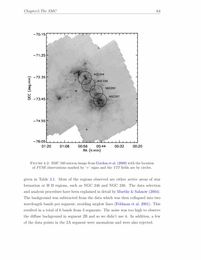
Chapter5:The SMC 64
Figure 4.2: SMC 160 micron image from Gordon et al. (2009) with the locationof FUSE observations marked by ‘+’ signs and the UIT fields are by circles.
given in Table 4.1. Most of the regions observed are either active areas of star
formation or H II regions, such as NGC 346 and NGC 330. The data selection
and analysis procedure have been explained in detail by Murthy & Sahnow (2004).
The background was subtracted from the data which was then collapsed into two
wavelength bands per segment, avoiding airglow lines (Feldman et al. 2001). This
resulted in a total of 6 bands from 3 segments. The noise was too high to observe
the diffuse background in segment 2B and so we didn’t use it. In addition, a few
of the data points in the 2A segment were anomalous and were also rejected.

Chapter5:The SMC 65
Figure 4.3: Correlation between the FUSE (1B1) and the UIT surface bright-ness is shown. The correlation coefficient is 0.88. The best fit line is withslope 0.72 and an offset of -10102.18 photons cm−2 s−1 sr−1 A−1. Errors in theobservations are small (relative to Y-axis scale) to be visible and are not shown.
Our target locations are marked with plus sign on an IR 160 micron (Gordon et
al. 2009) image of the SMC and the UIT fields are represented by circles (Figure
4.2). There is an excellent correlations exist between the FUSE bands with the
correlation coefficients better than 0.9 in each case. Our observed surface bright-
nesses (Table 4.1) extracted from the FUSE bands (1000 A– 1150 A) range from
a minimum of 1200 photons cm−2 s−1 sr−1 A−1 to as high as 2.5 × 10⁵ photons
cm−2 s−1 sr−1 A−1 in NGC 346, the youngest and largest H II region in the SMC.
We have estimated the level of Galactic background at these wavelengths from the
Voyager maps of Murthy et al. (1999) to be about 1000 photons cm−2 s−1 sr−1
A−1, below the FUSE detection limit.
We added observations from the UIT (Stecher et al. 1997) to extend our data into
the near UV. The UIT observed four 37′ diameter fields which encompassed most
of the bar of the SMC at 1615 A (Cornett et al. 1997) with an angular resolution

Chapter5:The SMC 66
of 3′′ (Figure 4.2). Nine of our FUSE targets fell within the area covered by the
UIT observations and we measured the diffuse UIT flux for them by rebinning the
1′′.13 UIT pixels over the 30′′x30′′ FUSE LWRS aperture. These fluxes are listed
in Table 4.1 and are highly correlated (r = 0.88) with the FUSE surface brightness
as shown in the Figure 4.3.
Most of the FUV diffuse targets are present on the Bar region of the SMC except
a bunch of bright FUV diffuse targets (nine targets) that are located in the north-
east of the SMC which is a supernovae remnant. Although this region is off the
SMC bar, we find this region very bright in UV. This is in close proximity to
the N66 which is the largest star forming region in the SMC with numerous O
type stars (Massey et al. 1989; Walborn et al. 2000) and also contains some of our
bright diffuse targets. It is likely that some part of the diffuse light comes from
the stars far away from the observed region where the dust grain is located. This
is evident from the calculations of Cole et al. (1999a) and Pradhan et al. (2010)
for the LMC where they found that much of the stellar radiation is non-local i.e.,
the diffuse light is actually the scattered light of distant stars by local dust. The
north-east region is bright in IR 160 micron as seen in figure 4.2 showing that
adequate amount of dusts are present which scatter the radiation from the OB
stars of N66.
4.2.1 Diffuse Fraction
The fraction of the total FUV light emitted as diffuse radiation in the SMC pro-
vides important information in context to the regional distribution of dust. UIT
observations cover the entire SMC bar (Figure 4.2) and Cornett et al. (1997) have
provided a catalog of all the UV stars in this region. We measured the total inte-
grated UV emission in the UIT images directly by summing the fluxes in pixels.
We used the catalog of Cornett et al. (1997) to calculate the total stellar emission
in each field at 1615 A. We extended the stellar emision into the FUSE bands
using the stellar radiation field model of Sujatha et al. (2004) that is based on
Kurucz models (Kurucz 1992) and calculated their emission in FUSE bands. We

Chapter5:The SMC 67
Figure 4.4: Variation of diffuse fraction against the wavelength for the UITregions as well as for the SMC bar as a whole. Dust albedo (dashed line) is fromthe model calculations of Weingartner & Draine (2001). The error bars wereempirically calculated by taking the extremes of the observed intensities andrange from 20% to 30% of the data. The model calculation of diffuse fraction
(dot-dashed line) is from Witt & Gordon (2000).
subtracted the total stellar emission from the integrated aperture emission to ob-
tain the total diffuse emission in each field which is the sum of contributions from
faint stars as well as dust scattered emissions. Cornett et al. (1997) predicted that
22% of the diffuse emission is contributed by the stars fainter than UV magnitude
14.5 at 1615 A. We measured the dust scattered diffuse light by subtracting the
faint star contribution. We extrapolated the diffuse emission into the FUSE bands
using the observed FUSE/UIT diffuse emission ratio, i.e., the slope of the best fit
line (Figure 4.3), obtained separately for each of the FUSE bands from their cor-
relation with UIT band. We used these to calculate the fraction of diffuse light
escaping the SMC, defined as the diffuse emission divided by the total emission
(diffuse + stellar), in each region and over the entire SMC bar (Figure 4.4) with
an estimated uncertainty of 20% – 30%. In all cases, the behaviour of the diffuse
fraction is almost the same, rising by 10% from 1000 A to 1150 A and a further

Chapter5:The SMC 68
Figure 4.5: Comparison of FUV diffuse fraction of the LMC and the SMC.The dashed line represents the albedo of the SMC and the dot-dashed linerepresents the albedo of the LMC and are obtained from the model calculations
of Weingartner & Draine (2001).
50% from 1150 Ato 1615 A, suggesting that the albedo of the dust increases by
about the same factor, in agreement with the theoretical predictions of Weingart-
ner & Draine (2001) for a mix of spherical carbonaceous and silicate grains over
the same wavelength range.
Integrating over the entire SMC bar, we find that 34% of the total radiation that
escapes the SMC bar at 1000 A is diffuse rising to 63% in the UIT bands at 1615
A. The scattered light in the SMC has been modelled by Witt & Gordon (2000)
using a multiple scattering code for a clumpy shell type dust geometry. The shell
geometry has stars extending to 0.3 of the system radius and dust extending from
0.3 to 1 of the syestem radius. They found that the ultraviolet scattered radiation
is in the range of 25% to 50% of the total integrated radiation coming from the
SMC bar. We have also plotted their modelled FUV scattered fraction along with
our observed fraction (Figure 4.4) which is agreeing the approximate observed

Chapter5:The SMC 69
value of diffuse fraction computed by us. Considering only H II regions of the
SMC, we found that around 20% of the total radiation at 1004A is diffuse rising
to 50% at 1615 A. Studies for the Orion nebula (Bohlin et al. 1982) and NGC
595 (Malumuth et al. 1996) find similar results with 66% of the total radiation
being diffuse at 1400 A in Orion and 55% at 1700 A in NGC 595. Pradhan et al.
(2010) found significantly smaller values for the diffuse fraction in the LMC (Figure
4.5) perhaps due to the difference in grain size and composition between the two
galaxies (Pei 1992; Weingartner & Draine 2001; Gordon et al. 2003). The albedo
of the SMC dust is about 50% higher (Weingartner & Draine 2001) compared to
the LMC dust (Figure 4.5) and this may explain the increased diffuse fraction in
the SMC.
The shape of the FUV diffuse fraction in both the LMC and the SMC are very much
similar in the wavelength range of 1000 Ato 1615 A but show regional variation
due to varying composition and distribution of dust as well as the variation 3of the
number density of young hot stars. We have examined the variation of the diffuse
fraction over different region in the SMC bar finding that it is larger in those areas
where there are fewer stars (NGC 267 and NGC 292) suggesting that much of the
diffuse radiation from those regions is actually due to distant stars. Similar results
were found in the LMC (Pradhan et al. 2010) which show that the diffuse fraction
is less in crowded regions such as 30 Doradus, SN 1987A and N11 (4% – 10%) and
more in sparse regions such as N70 (24% – 45%). Cole et al. (1999b) modeled the
escape fraction of NUV photons for the LMC where they show that much of the
stellar light is non-local i.e., the light from the distant OB associations is scattered
by local dust.
4.3 Correlation with the Hα Emission
The H II regions are accomplished copious Hα emitters with hot massive stars at
the center. The catalog of the H II regions in the SMC was given by Davies et al.
(1976) and the integrated Hα emission for them was calculated by Kennicutt &
Hodge (1986) defining circular aperture sizes. We have computed the integrated

Chapter5:The SMC 70
Figure 4.6: Plot of the FUV diffuse surface brightness and the Hα flux of theH II regions (Kennicutt & Hodge 1986). The best fit line is with slope 64.70and an offset of 1.30e-11 ergs cm−2 s−1 sr−1 A−1. The correlation coefficient is
0.81.
FUV diffuse emission at FUSE bands for 36 H II regions those were used by
Cornett et al. (1997). We found a good correlation with a correlation coefficient
of 0.81 between the integrated diffuse FUV emission and Hα emission from H II
regions of the SMC (Figure 4.6). This is as expected given that the Hα emission
is proportional to the brightness of the eciting stars as is FUV emission.
4.4 Conclusion
We have presented the first observations of FUV (1000 – 1150 A) diffuse radiation
from the SMC based on observations made with the FUSE. These targets are
present in various environments of the SMC. The diffuse radiation is primarily
due to light from hot stars scattered by the interstellar dust grains and ranges

Chapter5:The SMC 71
from around 103 photons cm−2 s−1 sr−1 A−1 to as high as 2.5 × 10⁵ photons cm−2
s−1 sr−1 A−1 in the SMC. The FUV diffuse fraction is 34% – 44% in the FUSE
bands (1000 – 1150 A) with a further increase upto 63% at 1615 A. Much less light
is scattered in the FUV than at long wavelengths showing that a large percent of
the light is absorbed by the dust. The FUV diffuse fraction emitted from the SMC
is much higher than the LMC which is attributed to the relatively higher value
of albedo of SMC dust compared to the LMC dust and less number of hot stars
in the SMC compared to the LMC. The FUV diffuse emission also corellates with
the Hα emission in the SMC.
We are now building a more detailed model to use the wealth of data now avail-
able in the MCs, particularly the data from Spitzer (Meixner et al. 2006). The
UV and IR data are complementary in that they probe different aspects of the
radiative transfer between stars and the dust with the part of the radiation not
scattered in the UV radiated in the IR and an understanding of the absorption
and subsequent re-emission of the starlight in a nearby galaxy such as the MCs
will provide templates for more distant galaxies where only the convolution of the
two is seen.

Chapter5:The SMC 72
Table 4.1: Details of FUSE observations in the SMC.
FUSE ID RA (LWRS) Dec(LWRS) LiF 1A1 LiF 1A2 LiF 1B1 LiF 1B2 UIT
G9310201 00 46 38.40 -73 08 24.0 1.33 ± 0.83 1.43 ± 0.36 1.56 ± 0.45 2.26 ± 0.53 16.02
G9310301 00 47 16.80 -73 08 24.0 0.97 ± 0.40 2.15 ± 0.22 2.56 ± 0.34 3.11 ± 0.38 32.96
G9310401 00 48 26.40 -73 19 12.0 2.78 ± 0.68 4.99 ± 0.29 6.62 ± 0.53 7.13 ± 0.65 24.69
G9310501 00 49 02.40 -73 14 24.0 3.28 ± 0.24 4.90 ± 0.13 5.78 ± 0.27 5.78 ± 0.24 18.90
G9310601 00 51 07.20 -73 21 36.0 9.07 ± 0.22 11.33 ± 0.11 11.09 ± 0.26 10.40 ± 0.28 13.57
F3230101 00 53 07.20 -74 39 00.0 3.87 ± 0.39 0.75 ± 0.63 0.48 ± 0.40 0.32 ± 0.29 4.19
F3230102 00 53 07.20 -74 39 00.0 0.15 ± 0.15 0.10 ± 0.09 0.28 ± 0.20 0.29 ± 0.23 7.84
F3230103 00 53 07.20 -74 39 00.0 0.87 ± 0.57 1.22 ± 0.40 0.94 ± 0.15 1.24 ± 0.15 11.25
F3230104 00 53 07.20 -74 39 00.0 0.12 ± 0.12 0.16 ± 0.11 0.27 ± 0.23 0.25 ± 0.14 7.61
F3230105 00 53 07.20 -74 39 00.0 0.15 ± 0.15 0.46 ± 0.32 0.40 ± 0.27 0.51 ± 0.27
F3230106 00 53 07.20 -74 39 00.0 0.25 ± 0.15 0.78 ± 0.06 0.64 ± 0.34 0.76 ± 0.23
D9110901 00 53 57.60 -70 37 48.0 0.22 ± 0.19 0.46 ± 0.41 0.22 ± 0.19 0.46 ± 0.41
G9310701 00 58 19.20 -72 17 24.0 10.07 ± 0.17 12.81 ± 0.10 13.69 ± 0.23 12.45 ± 0.22
P2030201 00 59 36.00 -72 07 48.0 17.03 ± 0.24 20.47 ± 0.17 25.15 ± 0.35 23.28 ± 0.36
C1580101 00 59 43.20 -72 09 36.0 3.50 ± 0.25 4.80 ± 0.13 5.72 ± 0.24 5.81 ± 0.30
S4057101 01 00 09.60 -72 08 24.0 8.96 ± 0.13 10.69 ± 0.07 9.63 ± 0.21 9.46 ± 0.18
G9310801 01 00 24.00 -71 33 36.0 5.78 ± 0.24 7.76 ± 0.16 9.35 ± 0.27 7.98 ± 0.34
G9310901 01 03 16.80 -72 09 36.0 15.90 ± 0.23 20.27 ± 0.12 22.02 ± 0.24 19.86 ± 0.22
G9311002 01 03 33.60 -72 02 24.0 20.30 ± 0.27 24.25 ± 0.14 25.15 ± 0.22 23.29 ± 0.28
C0830201 01 03 36.00 -71 58 48.0 14.64 ± 0.39 18.29 ± 0.17 16.64 ± 0.41 18.24 ± 0.41
G0350101 01 03 48.00 -71 58 12.0 5.31 ± 0.22 6.79 ± 0.12 7.67 ± 0.21 7.48 ± 0.25
E5110802 01 03 52.80 -72 54 00.0 2.69 ± 0.46 3.77 ± 0.20 4.41 ± 0.40 4.57 ± 0.44
F3210103 01 03 52.80 -72 07 48.0 17.09 ± 0.12 24.79 ± 0.07 34.14 ± 0.15 33.34 ± 0.14
F3210104 01 03 52.80 -72 07 48.0 22.18 ± 0.25 33.53 ± 0.11 46.05 ± 0.17 45.32 ± 0.21
E5110801 01 03 57.60 -72 54 36.0 0.70 ± 0.52 0.86 ± 0.45 0.92 ± 0.40 0.90 ± 0.50
A0750204 01 04 00.00 -72 01 48.0 24.65 ± 0.30 34.22 ± 0.16 30.03 ± 0.28 28.92 ± 0.27
C0830302 01 04 33.60 -71 59 24.0 2.97 ± 0.24 3.31 ± 0.17 2.92 ± 0.18 2.78 ± 0.19
G0350301 01 04 48.00 -72 01 12.0 8.17 ± 0.31 10.21 ± 0.17 9.93 ± 0.26 9.34 ± 0.40
D9044301 01 05 12.00 -72 23 24.0 0.95 ± 0.17 1.32 ± 0.08 0.55 ± 0.09 0.71 ± 0.12
D9044401 01 06 19.20 -72 05 24.0 1.85 ± 1.85 0.88 ± 0.27 1.64 ±1.20 0.78 ± 0.57
Notes. Units of right ascension are hours, minutes, and seconds; units of declina-
tion are in degrees, arc minutes and arc seconds. The diffuse surface brightness
in the FUSE and the UIT bands are in units of 104 photons cm−2 s−1 sr−1 A−1.

Chapter5:The SMC 73
The FUSE uncertainties are 1σ error bar and the error in the UIT data is around
10%.


Chapter 5
Survey of OVI in the Large
Magellanic Cloud
5.1 Introduction
The ISM of the MW and other galaxies is a complex mix of gas and dust. The
processes involved in maintaining the mass, energy, and ionization balance of the
ISM are not properly understood. The star and the ISM interact with each other
by which the stellar ecosystem is maintained. Stars are formed from the material in
the ISM and in turn stars also throw away a lots of mass to the ISM via cataclysmic
processes such as stellar winds and supernovae explosions that are accompanied
by release of a huge amount of energy which heats the ISM upto 106 degrees. This
superheated ISM is studied either by X-ray emissions or absorption lines of atoms
and ions produced via collisional ionization which fall in the ultraviolet wavelength
range of the electromagnetic spectrum. Five times ionized oxygen atom (O VI) is
one such ion produced in this environment and is a diagnostic of a temperatures of
about 3 × 10⁵ K (Cox 2005). Such temperatures are found at the interface of hot
(T > 106 K) and warm (T ∼ 104 K) ionized gas in the ISM. Thus, O VI absorption
lines at 1031.9 A and 1037.6 A are crucial diagnostics of the energetic processes
of interface environments in the ISM of galaxies. The gas at such temperatures
75
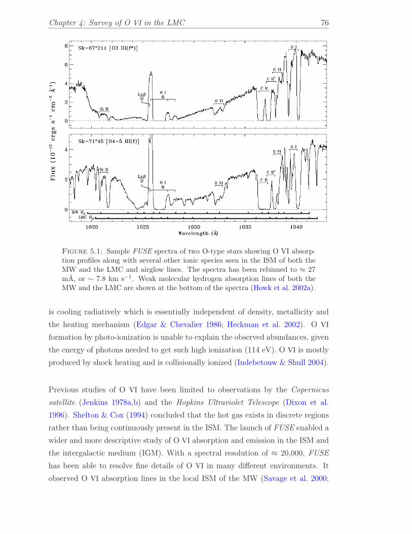
Chapter 4: Survey of O VI in the LMC 76
Figure 5.1: Sample FUSE spectra of two O-type stars showing O VI absorp-tion profiles along with several other ionic species seen in the ISM of both theMW and the LMC and airglow lines. The spectra has been rebinned to ≈ 27mA, or ∼ 7.8 km s−1. Weak molecular hydrogen absorption lines of both theMW and the LMC are shown at the bottom of the spectra (Howk et al. 2002a).
is cooling radiatively which is essentially independent of density, metallicity and
the heating mechanism (Edgar & Chevalier 1986; Heckman et al. 2002). O VI
formation by photo-ionization is unable to explain the observed abundances, given
the energy of photons needed to get such high ionization (114 eV). O VI is mostly
produced by shock heating and is collisionally ionized (Indebetouw & Shull 2004).
Previous studies of O VI have been limited to observations by the Copernicus
satellite (Jenkins 1978a,b) and the Hopkins Ultraviolet Telescope (Dixon et al.
1996). Shelton & Cox (1994) concluded that the hot gas exists in discrete regions
rather than being continuously present in the ISM. The launch of FUSE enabled a
wider and more descriptive study of O VI absorption and emission in the ISM and
the intergalactic medium (IGM). With a spectral resolution of ≈ 20,000, FUSE
has been able to resolve fine details of O VI in many different environments. It
observed O VI absorption lines in the local ISM of the MW (Savage et al. 2000;

Chapter 4: Survey of O VI in the LMC 77
Wakker et al. 2003; Oegerle et al. 2005; Savage & Lehner 2006; Welsh & Lallement
2008), disk of the MW (Bowen et al. 2008), halo of the MW (Savage et al. 2003),
the LMC (Howk et al. 2002a; Lehner & Howk 2007), the SMC (Hoopes et al. 2002),
starburst galaxies (Grimes et al. 2009), IGM (Danforth & Shull 2005; Danforth
et al. 2006), etc. Apart from absorption studies, FUSE has also recorded O VI
spectra in emission from observations of diffuse ISM in the MW (Shelton et al.
2001; Shelton 2002; Dixon et al. 2006; Dixon & Sankrit 2008) and superbubbles
in the LMC (Sankrit & Dixon 2007). These studies not only augmented our
knowledge about the formation and distribution of O VI in the MW and the MCs
but also helped in the understanding of the complexities of the ISM.
Figure 5.2: This is an R-band image of the LMC from Bothun & Thompson(1988) showing the 70 FUSE targets (‘+’ sign) towards which O VI absorptionhave been studied. Superbubbles are represented by circles with names aside.
Howk et al. (2002a) surveyed the distribution and kinematics of O VI towards
12 early type stars in the LMC, which was very selective and the targets were

Chapter 4: Survey of O VI in the LMC 78
restricted to Wolf-Rayet stars and O-type stars of spectral types O7 and earlier.
Figure 5.1 shows sample FUSE spectra of two O-type stars with target names SK-
67D211 and SK-71D45 respectively observed by Howk et al. (2002a). The O VI
doublet transitions at 1031.9 A and 1037.6 A are marked on the spectra along with
several other ionic absorption lines of both the MW and the LMC. The weaker
absorption of the O VI doublet at 1037.6 A is found to be inseparable from the C
II* and H2 absorption. The expected positions of the H2 lines for λ ≥ 1018 A and J
≤ 4 for both the LMC and the MW are marked under the spectrum. The (6-0)P(3)
and R(4) transitions of H2 at rest wavelengths of 1031.19 and 1032.35 respectively
can contaminate the O VI absorption at 1031.9 A. We report an extensive survey of
O VI absorption at 1032 A in the LMC. The observation log is given in Table 5.1.
The results presented in this survey become important as they not only provide
a detailed mapping of the interface gas traced by O VI but also throw light on
the small scale structure of the O VI distribution in various regions of the LMC.
Figure 5.2 shows the lines of sight and different regions of the LMC including the
superbubbles (marked by circles) that have been studied in this survey.
5.2 Observations and Data analysis
5.2.1 FUSE Data Analysis and Possible Contamination
The FUSE intrument is discussed in chapter 2 of this thesis. Depending on the
coating of the spectrograph, observations are possible through SiC and LiF chan-
nels that are further divided into eight different segments; the SiC 1A, SiC 2A, SiC
1B and SiC 2B segments covering the wavelength range 905A to 1105 A and LiF
1A, LiF 2A, LiF 1B and LiF 2B segments covering the wavelength range 1000A
to 1187 A. The data from SiC 2B segment have been known to suffer from a fixed
noise. The sensitivity of LiF 1A segment near 1032 A is almost double that of
other segments and therefore, we have used only the LiF 1A observations (Sahnow
et al. 2000). Most of the observations are from the LWRS with a few from the
MDRS aperture.

Chapter 4: Survey of O VI in the LMC 79
Figure 5.3: Examples of three sight lines showing the complexity of continuumfitting in the region near O VI absorption at 1031.92 A. The top to bottom
panels show the increasing complexity of fitting the stellar continuum.

Chapter 4: Survey of O VI in the LMC 80
The fully calibrated FUSE spectra were downloaded from the Multimission Archive
at STScI (MAST) processed by the latest FUSE data reduction pipeline (CAL-
FUSE version 3.2; Dixon et al. 2007). It made more than 600 pointings in and
around the LMC. Several of the observations were rejected initially due to either
non-existent or low signal-to-noise of O VI absorption profile in the spectra. 70
unique FUSE targets were selected based mainly on the simplicity of the con-
tinuum fitting in the vicinity of O VI (λ = 1031.9 A). Of the 70 targets, O VI
absorption for 1 of the sightline has been reported by Friedman et al. (2000), 11
have been covered by Howk et al. (2002a) survey, 3 by Danforth & Blair (2006a)
and 1 by Lehner & Howk (2007). Spectral types and other stellar information was
taken from Danforth et al. (2002) and Blair et al. (2009). We have downgraded all
the spectra reported here to 35 km s−1 to have a higher signal-to-noise. This has
been done for all the spectra irrespective of the quality to maintain uniformity in
the data analysis procedure.
Fitting of the stellar continuum in the neighbourhood of the O VI absorption
profile has been discussed in detail by Friedman et al. (2000) and Howk et al.
(2002a). Howk et al. (2002a) have limited their study to early type stars based
on the fact that these stars have completely developed O VI P Cygni profiles
that are easier to fit as the early type stars have a high mass loss rate and have
minimal wind variations. Lehner et al. (2001, 2003) have shown that for Galactic
sight lines, the stellar wind variability has negligible effect on O VI absorption
but may introduce substantial errors towards targets in the MCs. Lehner et al.
(2001) did find variation in the equivalent width and column density towards a
LMC star when estimated at two different times. This warrants for extra care
while fitting the continuum for MCs targets. As discussed above, for the LMC,
the estimation of stellar continuum in the vicinity of O VI absorption is not trivial.
Our background targets are mostly early O and B type stars with several Wolf-
Rayets. These have been selected based on the fact that the continuum near the
O VI absorption at 1031.9 A is simple to fit. A few of the lines of sight do show
a complex behaviour near O VI absorption (for e.g., Sk-67D05, Sk-67D168, Sk-
70D115, etc.). For such exceptional lines of sight, the complexity in the continuum
fitting is due to a local dip or a sudden rise near the O VI absorption and these
targets needed a comparatively higher order polynomial for the fitting. For a flavor
of the complexity involved, sample continuum fitting for three lines of sight, BI13,

Chapter 4: Survey of O VI in the LMC 81
Sk-70D115 and Sk-67D168 are shown in Figure 5.3. Following the fitting procedure
of Howk et al. (2002a) and Sembach & Savage (1992), the local stellar continuum
was estimated for all the targets and were fitted by a Legendre polynomial fit of
low order (≤ 5). Several continua were tested and the uncertainties involved for
the complete data set were used in the measurement of the O VI column densities.
The normalized spectra in the vicinity of O VI absorption are presented in Figure
5.10 (at the bottom of this chapter).
The O VI absorption may be contaminated by absorption from molecular hy-
drogen, however, it is minimal in the LMC velocity range. This is because the
molecular fraction of H2 in the LMC is only about 12% of the molecular fraction
in the Galactic disk (Tumlinson et al. 2002). The closest absorption line of H2 to
O VI absorption in the LMC lies at 1032.35 A (at vlsr ∼ +123 km s−1), which
is due to (6–0) R(4) transition. An estimation of possible contamination by H2
towards 12 lines of sight in the LMC has been done by Howk et al. (2002a) where
they find that H2 absorption does not affect the LMC O VI column densities sig-
nificantly. The H2 absorption feature are usually not a problem for measurements
of O VI absorption at velocities more than 20 km s−1 apart (Savage et al. 2003,
and reference therein). We estimate the contamination from H2 lines by fitting
the (6–0) P(3) H2 transition for the MW and (6–0) R(4) H2 transition for the
LMC (Figure 5.4). From this, we are able to estimate the contamination due to
(6–0) R(4) MW H2 line and (6–0) P(3) LMC H2 line. Noticeable contamination
is seen for the sightlines Sk-71D45 and Sk-67D250 which is well within the error
bar of the derived column densities. An example of a sightline is also shown in
Figure 5.4 in which the LMC O VI absorption is free from any contamination from
molecular hydrogen. Owing to the negligible contribution, we have not excluded
the contamination by H2 in the O VI measurements for the LMC.
Another possible contaminant is the (6–0) R(0) transition of the HD molecule
at 1031.91 A that overlaps with the MW O VI absorption. Several lines of HD
molecule is covered by FUSE and the complete list is given by Sembach (1999).
H2 column densities are significantly low in the LMC and contamination due to
molecular hydrogen lines is non-significant for O VI measurements in the LMC.

Chapter 4: Survey of O VI in the LMC 82
Figure 5.4: Model for H2 absorption overplotted on the normalized O VIabsorption profiles for 3 lines of sight. H2 absorption does not contaminatethe LMC O VI absorption for Sk-65D21, shows a maximum contamination for
Sk-71D45 and a moderate contamination for Sk-67D250.

Chapter 4: Survey of O VI in the LMC 83
Absorption due to HD is about 4 orders weaker compared to H2 transitions. There-
fore, we neglect any contribution from HD molecule to the column densities of O
VI in the LMC.
5.2.2 Measurement of O VI Column Densities
The measurement of equivalent widths and column densities of O VI absorption
for all the lines of sight were done following Savage & Sembach (1991); Sembach
& Savage (1992); Howk et al. (2002a). This apparent optical depth technique
(Savage & Sembach 1991) is now commonly used in the analysis of interstellar
absorption lines and is applicable to cases with non-saturated absorption profiles.
Briefly the technique uses an apparent optical depth in terms of velocity, i.e., an
instrumentally blurred version of the true optical depth, given as
τa(v) = ln[Io(v)/Iobs(v)], (5.1)
where Io is the estimated continuum intensity and Iobs is the intensity of the
absorption line as a function of velocity. If the resolution of the instrument is very
high compared to the FWHM of the absorption line, the apparent optical depth is
a very good representation of the true optical depth. The apparent column density
(Na(v) in atoms cm−2 (km s−1)−1) is calculated by the following relation
Na(v) =mecτa(v)
πe2fλ= 3.768 × 10¹⁴ τa(v)
fλ, (5.2)
where λ is the wavelength (A) and f is the oscillator strength of the atomic species
(for O VI, f value of 0.1325 has been adopted from Yan et al. 1998). Similar to
Howk et al. (2002a), we find that the 1032 A O VI profile is broad and is fully
resolved by FUSE. However, the weaker absorption of the O VI doublet at 1037.6
A is found to be inseparable from the C II* and H2 absorption.
The details of the apparent optical depth measurements are listed in Table 5.2.
The overlap of the O VI absorption of the MW and the LMC does not allow
a precise measurement of column densities for the LMC. For the lines of sight

Chapter 4: Survey of O VI in the LMC 84
(Sk-65D21, Sk-67D69, Sk-67D105, HV2543, Sk-66D100, HV5936, Sk-67D211, Sk-
69D220, Sk-66D172, Sk-68D137, D301-1005, and D301-NW8) where the LMC O
VI is distinct from the MW O VI, the limits of velocities over which integration
was performed were easy to obtain. Taking cue from these lines of sight, we
estimate the lower velocity limit for the lines of sight where the LMC O VI was
not separated from the MW O VI. The errors in the equivalent widths and column
densities are 1σ uncertainties derived using the uncertainty in the FUSE data and
the fitting procedures. The principal contributor to these errors is the ambiguity
in the continuum fitting of several of the spectra.
5.3 Distribution and Properties of O VI in the
LMC
5.3.1 Abundance and Linewidth of O VI
The LMC spectra were selected based on the quality of the spectra around O VI
spectral feature. The survey presented here has more-or-less complete coverage
of the well known regions of the LMC such as 30 Doradus, N11, LMC 4, etc.,
and thus, is very useful in studying the variation of O VI at small scales as well.
We find a significant amount of variation in the O VI column densities in a single
region and in different regions of the LMC.
Our data covers a wide range of targets; O type stars, B type stars, Wolf-Rayet
objects, supernova remnants (SNR), etc. The complete list of the background
targets is provided in Table 5.1. These observations give fine details of the small
scale structure of O VI column density in the LMC probing to a scale of ∼ 10
pc in some regions. We find the O VI absorption in the LMC to be very patchy
as is true for the MW. The O VI column density varies from the lowest value of
5.28 ×10¹³ atoms cm−2 near a H II region (DEM 7) to the highest value of 3.74
×1014 atoms cm−2 just north of the LMC bar. Howk et al. (2002a) report the
distribution of O VI in the LMC to be patchy as well with the log N(O VI) value
Chapter 4: Survey of O VI in the LMC 85
in the LMC varying from 13.9 to 14.6 atoms cm−2 and a mean of 14.37 atoms
cm−2. Their data did not provide any small scale variation in the column density
of O VI with the smallest scale probed is about 450–500 pc.
Given the coverage of our data, we have studied the variation in O VI absorption
in different regions of the LMC. We find that the 30 Doradus and SN 1987 A
regions dominate in terms of the abundance of O VI. The mean and median values
of log N(O VI) for targets in and around 30 Doradus and SNR 1987A are 14.30
and 14.27 atoms cm−2 respectively. 30 Doradus is the largest H II region of LMC
with a dense concentration of early type massive stars and has thus, attracted
extensive research in different wavelength bands (Walborn et al. 1992; Parker
1993; Malumuth & Heap 1994; Walborn & Blades 1997; Townsley et al. 2006;
Indebetouw et al. 2009). We discuss in detail about the O VI distribution and its
properties in 30 Doradus region in section 5.5. N11 region, which is associated
with several OB associations and has a superbubble at its center, shows a high
value of O VI column density. The mean of log N(O VI) in the N11 region is 14.21
atoms cm−2.
Another interesting region is the LMC 4 Supergiant shell that includes the Shapley
Constellation III, which is one of the largest region associated with star formation
(Dopita et al. 1985; Dolphin & Hunter 1998). The log N(O VI) value in LMC 4
supershell varies from a minimum of 13.86 atoms cm−2 to a maximum of 14.45
atoms cm−2 with a mean value of 14.20 atoms cm−2 and a median value of 14.25
atoms cm−2. Other regions of the LMC also show patchiness in the O VI distri-
bution. Statistically, the mean of the O VI column density in the LMC is 1.88
×1014 atoms cm−2 which is lower than 2.34 ×10¹⁴ atoms cm−2 given by Howk
et al. (2002a) for 12 lines of sight. The difference is most likely due to the wide
coverage of background targets in our data. The median value of the O VI column
density is 1.66 ×10¹⁴ atoms cm−2 which also is less than the value reported by
Howk et al. (2002a). Overall we find that there is an ubiquitous presence of O VI
throughout the LMC.
The kinematics of O VI in the LMC is difficult to study because of the ambiguity
in separating the LMC O VI absorption from the MW absorption. For some of

Chapter 4: Survey of O VI in the LMC 86
the FUSE targets, i.e., for Sk-65D21, Sk-67D69, Sk-67D105, HV2543, Sk-66D100,
HV5936, Sk-67D211, Sk-69D220, Sk-66D172, Sk-68D137, D301-1005, and D301-
NW8, O VI absorption at LMC velocities are distinct from the MW (Figure 5.10).
Linewidth for the LMC O VI profiles are obtained with relatively less error for
these lines of sight. The LMC O VI absorption profiles have all been fitted with a
single Gaussian. The corresponding FWHM for these lines of sight are 55, 85, 78,
90, 90, 113, 100, 85, 105, 94, 107, and 91 km s−1 respectively. The temperature
range estimated from these widths is T ∼ 1 × 10⁶ – 5 × 10⁶ K. O VI abundance
is maximum at a temperature of 3 × 10⁵ K, thus, higher FWHM of these profiles
is probably due to other broadening mechanisms such as more than one velocity
component and/or collision and turbulence. This also represents the kinematic
flow structure of O VI in the LMC.
The linewidth for the MW O VI profiles are narrower than the LMC profiles
(Savage et al. 2003; Oegerle et al. 2005; Savage & Lehner 2006). For the Galactic
halo, Savage et al. (2003) report a range for σ (linewidth) from 16 to 65 km s−1
(corresponding FWHM range is 38–153 km s−1). Oegerle et al. (2005), for the
local ISM, report average σ to be 16 km s−1 (FWHM = 38 km s−1) while Savage
& Lehner (2006) report σ values ranging from 15 km s−1 to 36 km s−1 (FWHM
ranging from 35 km s−1 to 85 km s−1). The linewidth of the SMC O VI absorption
profile are comparable to that of the LMC. The FWHM range for the SMC O
VI absorption is from 82 to 115 km s−1 with a mean of 94 km s−1 (Hoopes et al.
2002). We obtained a mean FWHM value of 91 km s−1 for the LMC selected lines
of sight. Howk et al. (2002a) have compared O VI absorption profiles of the LMC
with Fe II absorption and find that the Fe II profiles are much narrower suggesting
that the thermal broadening effect for O VI absorption is much more significant.
5.3.2 Comparison with the MW and the SMC
The MW and the SMC offer a different ISM environment compared to the LMC
especially due to the difference in the metallicity. The absorption profiles of the
MW O VI are different from the LMC O VI and sometimes these profiles are diffi-
cult to separate in an unambiguous manner, thus, a comparison of the kinematics

Chapter 4: Survey of O VI in the LMC 87
is not possible. Howk et al. (2002a) have compared the O VI absorption with Fe
II absorption at 1125.45 A. While, the Fe II profiles for the MW and the LMC are
clearly separated from each other, the O VI absorption suffers an overlap. This
is due to the difference in width of the two absorption. The overlap of the MW
O VI absorption profile with the LMC O VI absorption constrained Howk et al.
(2002a) to arrive at a definite conclusion about the existence of outflows from the
LMC. Following the discussion about the distribution of O VI in the LMC in the
previous section, we have presented an overview of O VI in the MW and the SMC.
O VI in the MW has been extensively studied since the launch of FUSE (Savage
et al. 2000; Howk et al. 2002b; Wakker et al. 2003; Savage et al. 2003; Oegerle et
al. 2005; Savage & Lehner 2006; Bowen et al. 2008). Savage et al. (2000) were the
first to study the O VI absorption in the disk and halo of the MW as seen towards
11 extragalactic objects (active galactic nuclei) using FUSE, confirming the large
scale presence of hot gas in the halo (Spitzer 1956). The authors find that log
N⊥(O VI) varies from 13.80 to 14.64 atoms cm−2 and the distribution of O VI is
quite patchy. To compare with the projected O VI column density on the plane
of the MW, we calculated the projection of O VI column on to the plane of the
LMC. Taking the inclination angle of the LMC to be 33, we find the mean value
of log N⊥(O VI) ≡ log N(O VI) cos θ = 14.16 atoms cm−2. Savage et al. (2000)
quote a mean value of 14.29 atoms cm−2 for their sample. The median value of
our sample is 14.14 atoms cm−2, while for the Savage et al. (2000) sample, it is
14.21 atoms cm−2.
Savage et al. (2003) report FUSE observations of O VI absorption towards 100
extragalactic lines of sight to study the properties and distribution of O VI in the
galactic halo. The average log N (O VI) for the complete sample is 14.36 atoms
cm−2 while log N (O VI) sin |b| value for the complete sample is 14.21 atoms
cm−2. The results reveal that there are substantial differences in the values of
log N(O VI) and log N(O VI) sin|b| in the northern Galactic hemisphere compared
to the southern Galactic hemisphere. The patchiness in the distribution of O VI
absorption is found to be similar over angular scales extending from ≤ 1 to 180.
An extensive survey of O VI in the MW disk has been reported by Bowen et al.
(2008) in which the authors have studied O VI column density towards 148 early

Chapter 4: Survey of O VI in the LMC 88
type stars. The correlation between O VI column density and effective distance to
a star establishes the fact that the O VI is interstellar in nature and points to the
universal presence of the interstellar phenomena that gives rise to O VI throughout
the Galaxy.
Hoopes et al. (2002) have surveyed O VI absorption towards 18 early type stars in
the SMC and report a widespread presence of O VI. The mean value of log N(O
VI) in the SMC is 14.53, which is higher than the LMC and the MW values. The
O VI column density in the SMC correlates with the distance from NGC 346, a
star forming region that shows the highest abundance of O VI in the SMC.
5.3.3 Comparison with X-ray and Hα
The LMC has been the focus of Hα and X-ray surveys to search for ionized struc-
tures in the ISM. Hα surveys have revealed the presence of H II regions, super-
nova remnants, and large scale structures including superbubbles and super-shells
(Davies et al. 1976), whereas, X-ray observations have studied bright X-ray sources
(Trumper et al. 1991), the hot gas in the ISM (Wang et al. 1989, 1991) and diffuse
X-ray emission (Bomans et al. 1994). Since O VI traces the ISM gas with tem-
peratures ∼ 105K, which is at the interface between hot gas (T ≥ 106K) traced
by X-rays and warm gas (T ∼ 104K) traced by Hα, correlation between O VI
abundance and X-ray and Hα emissions is expected.
The O VI observations cover specific regions of the LMC with varying environ-
mental conditions. To get an idea about the variation of O VI column densities
with different environments in the LMC, we have overlaid O VI column densities
as circles on Hα image (Gaustad et al. 2001, Figure 5.5). The diameter of the
circle is linearly proportional to log N(O VI). Interestingly, it is noted that O VI
abundance is high in regions with low Hα and X-ray emissions, i.e., regions that
are relatively inactive. However, regions like superbubbles are O VI rich, for e.g.,
30 Doradus C and N11. The gross picture suggests that O VI does not correlate
with either Hα or X-ray emissions. We have plotted log N(O VI) against log rela-
tive Hα and X-ray surface brightnesses to have a better insight. The X-ray surface

Chapter 4: Survey of O VI in the LMC 89
Figure 5.5: This is Hα image of the LMC from Gaustad et al. (2001) withcircles showing O VI absorption around the 70 targets. The diameter of thecircle is linearly proportional to the column density of O VI at LMC velocities.
brightness is obtained from ROSAT PSPC mosaic image of the LMC covering the
energy range 0.52.0 keV (Snowden & Petre 1994). Figure 5.6 and Figure 5.7 show
the correlation of log N(O VI) with Hα and X-ray surface brightnesses for the LMC
barring five lines of sight in the X-ray correlation plot. Four of the excluded lines
of sight (Sk-67D250, D301-1005, D301-NW8 and Sk-65D63) are not covered by
the X-ray observations and one (Sk-69D257) has extremely high X-ray emission
(about 2 orders of magnitude higher than other lines of sight). The Hα and X-ray
surface brightness are measured by rebinning the corresponding images to match
the FUSE LWRS and MDRS aperture size. The lack of correlation is evident in
both plots as it is found by Howk et al. (2002a). Since, Hα traces warm ISM and
star formation, there seems to be no direct relation between O VI formation and
these processes. A better correlation with X-ray is expected as the hot gas traced

Chapter 4: Survey of O VI in the LMC 90
0.0 0.5 1.0 1.5 2.0Log Relative H-alpha Surface Brightness
13.4
13.6
13.8
14.0
14.2
14.4
14.6
14.8L
og
N(O
VI)
Figure 5.6: log N(O VI)) vs. log relative Hα surface brightness for all the 70FUSE targets. Hα surface brightness is from Gaustad et al. (2001).
by X-ray is presumed to cool through temperatures where O VI formation takes
place. There is a high abundance of O VI in supernova remnants and superbubbles
of the LMC, whereas, bright X-ray emission is observed mostly from the supernova
remnants of the LMC. X-ray emission associated with supernova remnants in the
LMC is a factor of 2 to 3 times greater than the X-ray emission associated with
supergiant shells and the Bar in the LMC (Points et al. 2001).
5.4 O VI in superbubbles of the LMC
Superbubbles may be formed due to the strong stellar wind from young stars
and/or supernova explosions forming a local cavity in the surrounding ISM. These
are excellent examples of the interaction of young hot stars and the ISM. Super-
bubbles contain hot gas (∼ 106K) that is heated by shocks created by stellar

Chapter 4: Survey of O VI in the LMC 91
0.0 0.5 1.0 1.5 2.0 2.5Log Relative X-ray Surface Brightness
13.4
13.6
13.8
14.0
14.2
14.4
14.6
14.8
Lo
g N
(OV
I)
Figure 5.7: O VI column density (log N(O VI)) vs. log relative X-ray sur-face brightness for 65 targets. The X-ray surface brightness is taken from theROSAT PSPC mosaic image (energy range 0.5–2.0 keV) (Snowden & Petre1994). 4 targets (Sk-67D250, D301-1005, D301-NW8 and Sk-65D63) have notbeen covered by X-ray observations and one of the target Sk-69D257 has been
excluded because it has extremely high X-ray emission.
winds (Castor et al. 1975; Weaver et al. 1977; Chu & Mac Low 1990), which is
an ideal condition for the formation of O VI. The LMC hosts more than 20 su-
perbubbles and recently O VI has been detected in a superbubble N70 (Danforth
& Blair 2006a), where they have reported around 60% excess in abundance of O
VI in comparison to non-superbubble lines of sight in the proximity of N70. The
authors conclude that superbubbles act as local O VI reservoirs and have a differ-
ent absorption profile compared to the non-superbubble O VI absorption profiles.
They find that the O VI is formed by the thermal conduction between the inte-
rior hot X-ray producing gas and the cool photo-ionized shell of N70. Sankrit &
Dixon (2007) have detected O VI in emission in several superbubbles in the LMC
further emphasizing that superbubbles are important contributors to the overall
O VI budget.

Chapter 4: Survey of O VI in the LMC 92
We have 22 O VI observations covering 10 superbubbles as shown in Figure 5.1. Of
the 22 observations, 3 are in N70 (Sk-67D250, D301-1005 and D301-NW8) which
have already been reported by Danforth & Blair (2006a) and 4 are in N144, N204,
N206 and N154 respectively which have been discussed by Howk et al. (2002a). We
report 15 new observations of O VI absorption in the superbubbles 30 Doradus C,
N158, N11, N51, and N57. Significant variation in O VI abundance exists towards
these lines of sight. The minimum value of log N(O VI) is 14.04 atoms cm−2 in
superbubble N206 and the maximum value of log N(O VI) is 14.57 atoms cm−2
in superbubble N70. The properties of O VI in superbubbles reported here are
tabulated in Table 5.3. Comparing the abundance of O VI for the superbubble and
non-superbubble lines of sight, we find that the mean log N(O VI) for superbubble
lines of sight is 〈NSB〉 = 14.35 atoms cm−2 while for the non-superbubble lines of
sight this is 〈Nnon−SB〉 = 14.19 atoms cm−2. Thus, an excess O VI abundance of
about 40% in superbubbles of the LMC is found in comparison to non-superbubble
regions. Combining the Danforth & Blair (2006a) and Howk et al. (2002a) data
for superbubble and non-superbubble lines of sight (excluding Sk-67D05 sightline;
see Howk et al. (2002a) for details), the O VI excess in superbubbles is about
46%, which is comparable to our results. Thus, results reported here support
and confirm that superbubbles do show higher O VI abundance in comparison
to the general halo absorption seen in other LMC lines of sight. Some of the
non-superbubble lines of sight show an enhanced O VI column density owing to
local effects. Lehner & Howk (2007) compared superbubble and non-superbubble
lines of sight for the LMC and found that some quiescent environments showed an
enhanced O VI abundance, sometimes even larger than that of superbubbles.
Even in a single superbubble, there are significant variations in the O VI column
densities. We have four observations each for the superbubbles 30 Doradus C and
N11. In the case of 30 Doradus C, we find that the variation in N(O VI) is more
than a factor of 2 (from the minimum value of N(O VI) to the maximum value).
For N11, this variation is about a factor of 2.5. The variation in N(O VI) for N70
is not much (for the three lines of sight included here) and this corroborates with
the Danforth & Blair (2006a) data.

Chapter 4: Survey of O VI in the LMC 93
5.5 Properties of O VI in 30 Doradus
0.0 0.2 0.4 0.6 0.8 1.0Distance from center of R136 (degrees)
14.0
14.2
14.4
14.6
14.8L
og
N(O
VI)
Figure 5.8: Variation of O VI column density (log N(O VI)) with increasingdistance from the the centre of the star cluster R136 located in the 30 Doradusregion of the LMC. Note that the variation is plotted within an angular distance
of 1 degree from the the centre of R136.
The 30 Doradus region of the LMC is ideally suited to study the interaction
between a high rate of star formation and the surrounding ISM. This region is
dominated by the star forming cluster NGC 2070 that contains the very interesting
star cluster R136 at the center. The proximity to 30 Doradus has allowed extensive
research on the stellar content (Parker 1992; Parker & Garmany 1993a; Walborn
& Blades 1997) and initial mass function (Andersen et al. 2009, and the references
therein). 30 Doradus has also been investigated in detail in the infrared bands
to study the dust properties (Sturm et al. 2000; Vermeij et al. 2002; Meixner et
al. 2006). Indebetouw et al. (2009) studied the 30 Doradus in the mid-infrared
wavelength band to determine the physical conditions of the ionized gas and found
that the local effects of hot stars in 30 Doradus appear to dominate over any large-
scale trend with distance from the central cluster R136.

Chapter 4: Survey of O VI in the LMC 94
0.5 1.0 1.5 2.0 2.5Log Relative X-ray Surface Brightness
14.0
14.2
14.4
14.6
14.8L
og
N(O
VI)
Figure 5.9: O VI column density (log N(O VI)) vs. X-ray luminosity forthe 30 Doradus region of the LMC. The X-ray surface brightness is taken fromthe ROSAT PSPC mosaic image (energy range 0.5–2.0 keV) (Snowden & Petre1994). A linear correlation is present which is not seen when all the targets ofLMC are included (Figure 5.7) and for other individual regions in the LMC.The plot includes all lines of sight from Figure 5.8 except for 1 sightline (SK-69D257) as it shows an exceptionally high X-ray emission due to its proximity
to X-ray binary LMC-X1 (Points et al. 2001).
The O VI abundance in 30 Doradus is higher than in other regions of the LMC
with the highest value of log N(O VI) being 14.56 atoms cm−2 near the center of
the cluster R136. Figure 5.8 shows the change in the log N(O VI) values from
the center of R136 up to an angular distance of 1 degree. We find an overall
decrease in the O VI abundance away from the center of R136. An interpretation
of this plot could be that the processes involved in the formation of O VI are likely
to be associated with stellar radiation field but local effects cannot be neglected
on a large angular scale. It should be noted that we do not find any correlation
between O VI absorption and Hα emission for LMC and thus, no relation between
star formation is established on a larger scale.

Chapter 4: Survey of O VI in the LMC 95
As noticed earlier, log N(O VI) does not correlate with X-ray emission for the LMC
as a whole but surprisingly there is a good correlation for the 30 Doradus lines
of sight Figure 5.9. The correlation is between log N(O VI) and X-ray emission
from 30 Doradus considering all the lines of sight within 1 degree around R136
except for one sightline (SK-69D257) that has exceptionally high value of X-ray
surface brightness. One of the reasons for such high X-ray emission from SK-
69D257 is its proximity to a high mass X-ray binary LMC X-1 (Points et al.
2001). The correlation in 30 Doradus suggests that O VI observed in this region is
present in the ISM gas surrounding the X-ray emitting plasma, which may be due
to the compactness, high density and non-uniform structure of 30 Doradus. The
correlation confirms that the X-ray emitting gas cools through temperatures where
O VI is being formed and supports the general consensus about the formation of
O VI by collisional ionization in the interface regions between cooler photo-ionized
ISM gas and hot exterior ISM gas (Slavin & Frisch 2002; Indebetouw & Shull
2004).
5.6 Summary & Conclusions
We have presented O VI column density measurements for the LMC using FUSE
data for 70 lines of sight. This is the widest coverage of the LMC to date. The
results reported here reveal significant variation in O VI column densities over a
very small angular scale thus confirming the patchiness of O VI distribution in the
LMC. The most important inferences drawn from this work are following:
1. This survey probes 70 lines of sight with varying environmental conditions.
We find strong O VI absorption in the LMC that is not restricted to active
regions. High O VI abundance is present even in relatively inactive regions
of the LMC.
2. There are significant variations in the velocity profiles of O VI absorption.
The O VI absorption profile is broader than the MW absorption for many
lines of sight but it should be noted that unambiguous separation of the MW

Chapter 4: Survey of O VI in the LMC 96
and the LMC components is not possible for most of the lines of sight. This
proves to be a significant hurdle in interpreting exact kinematics for O VI in
the LMC (for e.g. outflows from the LMC, etc.).
3. The maximum column density measured for the LMC is log N(O VI) = 14.57
atoms cm−2 and minimum value is log N(O VI) = 13.72 atoms cm−2. The
mean value of O VI column density is <log N(O VI)> = 14.23 atoms cm−2,
which is slightly lower than the earlier reported value. The median value of
O VI column density in the LMC comes to be 14.22 atoms cm−2. The results
corroborates with the previous finding that the distribution of O VI in the
LMC is patchy.
4. Despite the fact that the LMC has lower metallicity than the MW, the
abundance of O VI and properties of O VI absorption are similar in both the
galaxies. The mean of log N⊥(O VI) value for the MW is 14.29 atoms cm−2
while the projected column density for the LMC, i.e., log N⊥(O VI) is 14.15
atoms cm−2. A more extensive study for the MW suggests this value to be
14.21 atoms cm−2. The SMC with even lower metallicity has higher O VI
abundance with mean log N(O VI) = 14.53 atoms cm−2.
5. O VI absorption in the LMC does not correlate with Hα (warm gas) or X-ray
(hot gas) emission but we find a good correlation between O VI absorption
and X-ray emission in the 30 Doradus region. It is also seen that the O
VI absorption is decreasing with increasing angular distance from the star
cluster R136 suggesting some correlation with stellar radiation field.
6. The observations reported cover 10 superbubbles of the LMC and for 5 su-
perbubbles (30 Doradus C, N158, N51, N11 and N57) O VI absorption is
reported for the first time. Superbubbles are O VI rich and have 40% excess
compared to non-superbubble lines of sight.

Chapter 4: Survey of O VI in the LMC 97
(a) Normalized OVI absorption profiles.

Chapter 4: Survey of O VI in the LMC 98
(b) Normalized OVI absorption profiles.

Chapter 4: Survey of O VI in the LMC 99
(c) Normalized OVI absorption profiles.

Chapter 4: Survey of O VI in the LMC 100
(d) Normalized OVI absorption profiles.

Chapter 4: Survey of O VI in the LMC 101
(e) Normalized OVI absorption profiles.

Chapter 4: Survey of O VI in the LMC 102
(f) Normalized OVI absorption profiles.
Figure 5.10: Normalized O VI absorption profiles for the 70 lines of sight.

Chapter 4: Survey of O VI in the LMC 103
Table 5.1: Log of FUSE observations for the 70 targets in the LMC.
FUSE ID Object name Aperture Right Ascension Declination Spec Type V mag. Ref
P1030703 Sk-67D05 LWRS 04 50 18.96 -67 39 37.9 O9.7Ib 11.34 1
A0490402 Sk-68D03 LWRS 04 52 15.56 -68 24 26.9 O9I 13.13 2
E5111901 BI13 LWRS 04 53 06.48 -68 03 23.1 O6.5V 13.75 3
D0980801 Sk-67D18 MDRS 04 55 14.90 -67 11 24.5 O6-7n-nm 11.95 1
P1174401 Sk-67D20 LWRS 04 55 31.50 -67 30 01.0 WN4b 13.86 4
B0100201 PGMW-3070 MDRS 04 56 43.25 -66 25 02.0 O6V 12.75 5
D0300302 LH103102 MDRS 04 56 45.40 -66 24 45.9 O7Vz 13.55 5
D0300101 LH91486 MDRS 04 56 55.58 -66 28 58.0 O6.5Vz 14.2 5
B0100701 PGMW-3223 MDRS 04 57 00.80 -66 24 25.3 O8.5IV 12.95 5
F9270604 HV2241 LWRS 04 57 15.83 -66 33 54.8 O7-III 13.5 5
P1174901 HD32402 LWRS 04 57 24.19 -68 23 57.2 WC 3
Z9050801 Sk-67D32 LWRS 04 59 52.30 -67 56 55.0 WN 14.48 3
P1030901 Sk-65D21 LWRS 05 01 22.33 -65 41 48.1 O9.7Iab 12.02 6
B0770201 HV2274 LWRS 05 02 40.96 -68 24 21.3 B0-B2III-I 14.2 5
P1174501 Sk-66D51 LWRS 05 03 10.20 -66 40 54.0 WN8h 12.71 4
D1380201 NGC1818-D1 LWRS 05 04 32.56 -66 24 51.0 B0-B2V-IV 14.93 5
P1172101 Sk-70D69 LWRS 05 05 18.73 -70 25 49.8 O5V 13.94 6
P1171703 Sk-67D69 LWRS 05 14 20.16 -67 08 03.5 O4III(f) 13.09 7
C1030101 MACHO78-6097 LWRS 05 18 04.70 -69 48 19.0 B0-B2V-IV 14.4 5
E5112902 BI130 LWRS 05 18 06.06 -69 14 34.5 O8.5V((f)) 12.53 3
Z9050201 Sk-69D94 LWRS 05 18 14.53 -69 15 01.0 B0-B2III-I 9.72 5
D9044701 SNR0519-697 LWRS 05 18 44.20 -69 39 12.4 SNR
D0880104 BREY22 MDRS 05 19 16.40 -69 39 19.5 WC/O9.5Ib 12.3 1
B0270101 HD269445 LWRS 05 22 59.87 -68 01 46.6 WN 11.45 1
P1173602 Sk-69D124 LWRS 05 25 18.37 -69 03 11.1 O9Ib 12.81 2
D1530104 Sk-67D105 LWRS 05 26 06.37 -67 10 57.6 Of 12.42 5
A1110101 Sk-67D106 MDRS 05 26 15.20 -67 29 58.3 B0-B2III-I 11.78 8
A1110201 Sk-67D107 MDRS 05 26 20.67 -67 29 55.4 B0-B2III-I 12.5 8
C1510101 HD36521 LWRS 05 26 30.32 -68 50 25.4 WC 12.42 9
P1031402 Sk-68D80 LWRS 05 26 30.43 -68 50 26.6 WC4+OB 12.40 10
P2030104 Sk-68D82 LWRS 05 26 45.31 -68 49 52.8 WN5?b+(B3I) 9.86 5
P1173701 BI170 LWRS 05 26 47.79 -69 06 11.7 O9.5Ib 13.09 11
C1550201 Sk-67D111 LWRS 05 26 47.95 -67 29 29.9 O6:Iafpe 12.57 11
F9270701 HV2543 LWRS 05 27 27.40 -67 11 55.4 O8+O9 12.92 5
P1172501 Sk-70D91 LWRS 05 27 33.74 -70 36 48.3 O6.5V 12.78 11
P1172303 Sk-66D100 LWRS 05 27 45.59 -66 55 15.0 O6II(f) 13.26 6
E9570301 HDE269599 LWRS 05 28 22.68 -69 08 32.2 Be 10.18 5
Continued on Next Page. . .

Chapter 4: Survey of O VI in the LMC 104
Table 5.1 – Continued
FUSE ID Object name Aperture Right Ascension Dec Spectral Type V mag. Ref
M1142001 Sk-65D63 LWRS 05 28 39.50 -65 39 01.1 O9.7I 12.56 12
C1030201 HV982 LWRS 05 29 52.50 -69 09 22.0 B0-B2V-IV 14.6 5
E5113602 Sk-70D97 LWRS 05 30 11.35 -70 51 42.2 O9III 13.33 5
P1175001 Sk-67D144 LWRS 05 30 12.22 -67 26 08.4 WC4+OB 13.6 13
P2170301 BI184 LWRS 05 30 30.60 -71 02 31.3 B0-B2V-IV 13.84 3
D1380301 NGC2004-B15 MDRS 05 30 36.58 -67 17 42.3 B0-B2V-IV 14.18 5
Z9050601 Sk-71D38 LWRS 05 30 38.77 -71 01 47.9 WC 13.1 5
P1031502 Sk-71D45 LWRS 05 31 15.55 -71 04 08.9 O4-5III(f) 11.51 1
A1330123 Sk-67D166 LWRS 05 31 44.31 -67 38 00.6 O4If+ 12.27 1
B0860901 Sk-67D168 MDRS 05 31 52.10 -67 34 20.8 O8Iaf 12.08 12
D9042002 SNR0532-675 LWRS 05 32 23.00 -67 31 02.0 SNR
P1173101 Sk-67D191 LWRS 05 33 34.12 -67 30 19.6 O8V 13.46 2
B0770302 HV5936 LWRS 05 33 39.00 -66 37 39.8 B0-B2V-IV 14.8 5
P1175101 Sk-69D191 LWRS 05 34 19.39 -69 45 10.0 WC4 13.35 13
F3210301 J053441-693139 LWRS 05 34 41.30 -69 31 39.0 O2-O3.5If* 13.7 14
P1171603 Sk-67D211 LWRS 05 35 13.92 -67 33 27.0 O2III(f)* 12.28 14
Z9051001 BREY64 LWRS 05 35 54.45 -68 59 07.4 WN9h 13.21 3
D9043101 SNR0536-692 LWRS 05 36 07.70 -69 11 52.6 SNR
Z9050701 Sk-69D220 LWRS 05 36 43.83 -69 29 47.4 WNorOiafpe 10.58 1
P1172201 Sk-66D172 LWRS 05 37 05.56 -66 21 35.7 O2III(f)*+OB 13.13 14
C0020601 BI253 LWRS 05 37 34.49 -69 01 09.8 Of 13.76 3
E5114201 Sk-68D137 LWRS 05 38 24.77 -68 52 32.8 O3IIIf 13.29 3
P1171803 MK42 LWRS 05 38 42.10 -69 05 54.7 O3If/WN6-A 10.96 15
P1031706 Sk-69D243 LWRS 05 38 42.57 -69 06 03.2 WN5+OB 9.5 16
F9140101 30DOR-S-R136 LWRS 05 38 51.70 -69 06 00.0 H II region
P1031802 Sk-69D246 LWRS 05 38 53.50 -69 02 00.7 WN 11.16 4
P1174601 HDE269927 LWRS 05 38 58.25 -69 29 19.1 WN 12.63 4
P2170101 Sk-69D257 LWRS 05 39 58.91 -69 44 03.2 O9II 12.53 5
D9042801 SNR0543-689 LWRS 05 43 07.20 -68 58 52.0 SNR
D0981401 D301-1005 MDRS 05 43 08.30 -67 50 52.4 O9.5V 14.11 3
D0981201 Sk-67D250 MDRS 05 43 15.48 -67 51 09.6 O7.5II(f) 12.68 17
D0981501 D301-NW8 MDRS 05 43 15.96 -67 49 51.0 D301-NW8 14.37 3
I8120701 Sk-70D115 LWRS 05 48 49.76 -70 03 57.5 O6.5Iaf 12.24 5
Notes. Units of right ascension are hours, minutes, and seconds; units of declination are in
degrees, arcminutes and arcseconds.
References – (1) Walborn (1977); (2) Conti et al. (1986); (3) Massey (2002); (4) Smith et al.
Chapter 4: Survey of O VI in the LMC 105
(1996); (5) Blair et al. (2009); (6) Walborn et al. (1995); (7) Garmany & Walborn (1987) (8)
Rousseau et al. (1978); (9) Moffat et al. (1990); (10) Smith et al. (1990); (11) Walborn et al.
(2002b) (12) Fitzpatrick & Massa (1988); (13) Torres-Dodgen & Massey (1988); (14) Walborn
et al. (2002a); (15) Walborn & Blades (1997); (16) Massey & Hunter (1998); (17) Massey et al.
(1995).

Chapter 4: Survey of O VI in the LMC 106
Table 5.2: Equivalent widths and column densities with corresponding velocity
limits over which the integration is performed for O VI absorption in the LMC.
Target name Equivalent width log N(O VI) Integration limits
(mA) (dex) (km s−1)
Sk-67D05 73±6 13.72+0.10−0.13 175, 330
Sk-68D03 112±8 14.02+0.11−0.15 180, 330
BI13 88±4 13.94+0.08−0.09 175, 315
Sk-67D18 132±7 14.16+0.09−0.13 165, 330
Sk-67D20 147±8 14.08+0.11−0.16 175, 335
PGMW-3070 132±23 14.10+0.13−0.18 180, 345
LH103102 132±23 14.16+0.03−0.04 180, 330
LH91486 266±29 14.47+0.09−0.11 175, 385
PGMW-3223 129±15 14.10+0.06−0.07 175, 315
HV2241 271±18 14.50+0.04−0.03 165, 365
HD32402 271±8 14.48+0.02−0.02 160, 320
Sk-67D32 129±7 14.11+0.03−0.04 165, 360
Sk-65D21 94±23 13.94+0.11−0.16 225, 340
HV2274 160±11 14.14+0.10−0.15 165, 345
Sk-66D51 185±10 14.26+0.07−0.09 170, 370
NGC1818-D1 280±13 14.52+0.05−0.05 150, 340
Sk-70D69 182±12 14.18+0.07−0.08 150, 295
Sk-67D69 232±28 14.40+0.05−0.06 170, 340
MACHO78-6097 151±25 14.15+0.05−0.05 165, 320
BI130 94±7 13.89+0.07−0.09 165, 320
Sk-69D94 150±3 14.22+0.03−0.03 160, 340
SNR0519-697 97±4 13.97+0.07−0.08 160, 300
BREY22 126±24 14.07+0.06−0.07 160, 330
HD269445 200±10 14.29+0.04−0.05 175, 365
Sk-69D124 331±8 14.57+0.04−0.05 190, 430
Sk-67D105 110±8 13.92+0.14−0.23 180, 320
Sk-67D106 180±7 14.30+0.10−0.13 175, 345
Sk-67D107 254±10 14.45+0.04−0.05 160, 360
Continued on Next Page. . .

Chapter 4: Survey of O VI in the LMC 107
Table 5.2 – Continued
Target name Equivalent width log N(O VI) Integration limits
(mA) (dex) (km s−1)
HD36521 126±9 14.07+0.09−0.12 175, 340
Sk-68D80 303±16 14.56+0.04−0.03 145, 335
Sk-68D82 141±10 14.17+0.04−0.04 165, 320
BI170 235±20 14.43+0.02−0.03 165, 365
Sk-67D111 214±19 14.34+0.05−0.05 175, 365
HV2543 156±42 14.23+0.04−0.03 160, 365
Sk-70D91 256±7 14.43+0.04−0.03 160, 365
Sk-66D100 214±21 14.34+0.03−0.03 160, 340
HDE269599 123±6 14.05+0.03−0.03 165, 320
Sk-65D63 184±8 14.21+0.04−0.04 180, 375
HV982 208±58 14.33+0.12−0.17 175, 360
Sk-70D97 226±4 14.39+0.03−0.04 175, 375
Sk-67D144 194±10 14.25+0.06−0.07 165, 335
BI184 118±10 14.04+0.08−0.10 165, 330
NGC2004-B15 92±7 13.86+0.05−0.07 175, 330
Sk-71D38 94±7 13.92+0.07−0.08 165, 315
Sk-71D45 194±9 14.26+0.06−0.06 160, 345
Sk-67D166 206±9 14.32+0.05−0.05 165, 390
Sk-67D168 186±12 14.26+0.05−0.05 165, 375
SNR0532-675 147±9 14.16+0.07−0.08 165, 345
Sk-67D191 229±16 14.42+0.02−0.02 165, 340
HV5936 174±8 14.18+0.07−0.08 175, 375
Sk-69D191 185±25 14.22+0.06−0.07 165, 340
J053441-693139 182±33 14.22+0.05−0.05 165, 330
Sk-67D211 144±8 14.11+0.10−0.13 160, 350
BREY64 139±8 14.20+0.16−0.23 180, 330
SNR0536-692 116±7 14.03+0.05−0.07 165, 320
Sk-69D220 128±9 14.09+0.08−0.11 160, 315
Sk-66D172 173±9 14.20+0.05−0.05 175, 360
BI253 259±46 14.46+0.04−0.05 160, 300
Continued on Next Page. . .
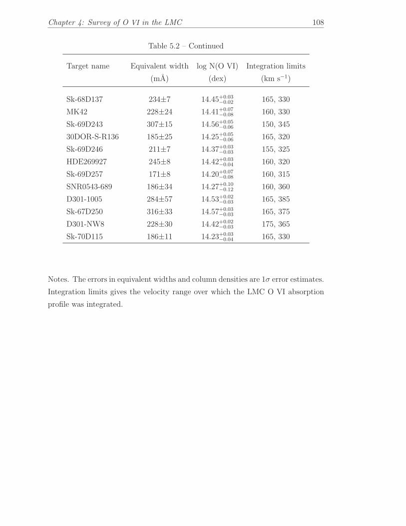
Chapter 4: Survey of O VI in the LMC 108
Table 5.2 – Continued
Target name Equivalent width log N(O VI) Integration limits
(mA) (dex) (km s−1)
Sk-68D137 234±7 14.45+0.03−0.02 165, 330
MK42 228±24 14.41+0.07−0.08 160, 330
Sk-69D243 307±15 14.56+0.05−0.06 150, 345
30DOR-S-R136 185±25 14.25+0.05−0.06 165, 320
Sk-69D246 211±7 14.37+0.03−0.03 155, 325
HDE269927 245±8 14.42+0.03−0.04 160, 320
Sk-69D257 171±8 14.20+0.07−0.08 160, 315
SNR0543-689 186±34 14.27+0.10−0.12 160, 360
D301-1005 284±57 14.53+0.02−0.03 165, 385
Sk-67D250 316±33 14.57+0.03−0.03 165, 375
D301-NW8 228±30 14.42+0.02−0.03 175, 365
Sk-70D115 186±11 14.23+0.03−0.04 165, 330
Notes. The errors in equivalent widths and column densities are 1σ error estimates.
Integration limits gives the velocity range over which the LMC O VI absorption
profile was integrated.

Chapter 4: Survey of O VI in the LMC 109
Table 5.3: O VI column densities in the superbubbles (SB) of the LMC.
Target name Superbubble Column density log N(O VI)(1014 atoms cm−2) (dex)
Sk-69D246 30Dor C 2.36+0.18−0.14 14.37+0.03
−0.03
MK42 30Dor C 2.60+0.46−0.45 14.41+0.07
−0.08
30DOR-S-R136 30Dor C 1.77+0.20−0.24 14.25+0.05
−0.06
Sk-69D243 30Dor C 3.63+0.40−0.45 14.56+0.05
−0.06
Sk-69D191 N154 1.65+0.26−0.23 14.22+0.06
−0.07
HDE269927 N158 2.62+0.16−0.21 14.42+0.03
−0.04
Sk-68D80 N144 3.61+0.30−0.26 14.56+0.04
−0.03
HD36521 N144 1.18+0.28−0.28 14.07+0.09
−0.11
BI184 N206 1.09+0.22−0.22 14.04+0.08
−0.10
Sk-71D45 N206 1.80+0.24−0.21 14.26+0.06
−0.06
Sk-70D91 N204 2.69+0.24−0.17 14.43+0.04
−0.03
PGMW-3223 N11 1.27+0.18−0.18 14.10+0.06
−0.07
LH103102 N11 1.46+0.10−0.13 14.16+0.03
−0.04
PGMW-3070 N11 1.27+0.43−0.43 14.10+0.13
−0.18
LH91486 N11 2.96+0.68−0.68 14.47+0.09
−0.11
Sk-67D111 N51 2.20+0.29−0.24 14.34+0.05
−0.05
Sk-67D107 N51 2.85+0.27−0.27 14.45+0.04
−0.05
Sk-67D106 N51 2.01+0.50−0.53 14.30+0.10
−0.13
Sk-67D166 N57 2.09+0.25−0.20 14.32+0.05
−0.05
Sk-67D250 N70 3.71+0.23−0.23 14.57+0.03
−0.03
D301-1005 N70 3.37+0.17−0.22 14.53+0.02
−0.03
D301-NW8 N70 2.60+0.09−0.13 14.42+0.02
−0.03
Total SB (this work) 2.31±0.12 14.35±0.18Total non-SB (this work) 1.68±0.12 14.19±0.23Total SB N701 3.04±0.45 14.48±0.06Total non-SB1 2.03±0.58 14.29±0.14Total SB2 3.07±0.62 14.48±0.09Total non-SB2 2.10±0.50 14.31±0.11
Notes. The superbubble lines of sight are shown in Figure 5.1.
(1) Danforth & Blair (2006a); (2) Combined data of Howk et al. (2002a) and
Danforth & Blair (2006a).


Chapter 6
Summary & Conclusions
6.1 Summary
The ISM is the space between stars consisting of atoms, molecules and ionized
gases at various temperatures and dust grains that contain a large fraction of the
elements heavier than hydrogen and helium. Although dust grains account for
only 1% of the mass of the ISM, these are observed in every line of sight obscuring
stars and galaxies. Therefore, the analysis of spectra of celestial objects requires
a proper understanding of the physical and chemical properties of the ISM and
in particular the interstellar dust. Most of the energy input into the dust comes
from energetic UV photons emitted by hot young stars (Law et al. 2011). A part
of the stellar UV radiation is scattered by interstellar dust, which is observed as
diffuse UV radiation and the rest is absorbed and re-emitted in the IR wavelength
band of the electromagnetic spectrum. We have given an overview of the dust
grain properties such as extinction, emission, absorption, scattering, polarization
and distribution, and the properties of gas components at different temperatures
with a brief description of their detection methods in chapter 1.
The Magellanic Clouds are interesting nearby extra-galactic objects to investigate
the connection between starlight and diffuse light as well as the properties of the
111

Chapter6: Summary 112
dust and gas in the ISM condition with low metallicity and under abundance of
dust. The ISM of the MCs can be treated as relatively primitive because of its low
metallicty and can be the stepping stone in our understanding of the ISM in high
red-shift galaxies. We have presented the first observations of the FUV diffuse
emission (1000 A– 1150 A) from the MCs that is dependent on both the amount
of starlight and the relative geometry of the dust and the stars.
Diffuse UV light is dominated by radiation from hot stars scattered by interstellar
dust grains. The intensity of this background radiation depends on the distribution
of hot stars, amount and distribution of dust grains, optical depth and the optical
parameters of dust. Chapter 2 provides a comprehensive literature survey on
FUV diffuse background radiation and discusses about the various components of
it. We have also described the data reduction method (Murthy & Sahnow 2004)
that is employed to extract the diffuse surface brightness from the FUSE spectra
and presented the first observations of FUV diffuse emission for the MCs. A brief
description of the FUSE instrument along with the data reduction techniques are
also given in Chapter 2.
81 bright FUV diffuse observations in the LMC are reported in Chapter 3. Most of
these observation are near OB associations. The intensities of these observations
range from around 103 photons cm−2 s−1 sr−1 A−1 to as high as 3 × 10⁵ photons
cm−2 s−1 sr−1 A−1 at FUSE bands with negligibly small contribution from the
Galactic diffuse radiation. A good correlation between the FUSE diffuse radiation
and the diffuse radiation measured from the UIT exists. Based on this correlation,
and using the stellar catalog of Parker et al. (1998), we have estimated the fraction
of diffuse radiation emanating from the LMC. These fractions vary in different
regions of the LMC. The fractions range from 5% to 20% of the total integrated
emission at 1100 A, with a high of 45% in the superbubble N70, and with an
observed error of 12% – 17%. The shape of the diffuse fraction is same in all the
10 UIT regions rising by a factor of about 5 from 1000 Ato 1500 A, suggesting
that most of the heating of the interstellar dust comes in the FUV in the LMC is
shown by Law et al. (2011) for starburst galaxies.
We report 30 diffuse observations in various environments of the SMC in Chapter

Chapter6: Summary 113
4. These observations cover different regions of the SMC with several near hot
stars of the bar region to regions further out in the edges of the galaxy. The
strength of these diffuse signals range from around 103 photons cm−2 s−1 sr−1
A−1 to as high as 2.5 × 10⁵ photons cm−2 s−1 sr−1 A−1. We estimated the FUV
diffuse fraction in the SMC and found significant variations in different regions.
The diffuse FUV fraction ranges between 34% – 44% in the FUSE bands (1000
– 1150 A) with a further increase upto 63% at 1615 A. In case of the SMC, the
behaviour of the diffuse fraction is almost the same as the LMC, rising by 10%
from 1000 A to 1150 A and a further 50% from 1150 Ato 1615 A, suggesting
that the albedo of the dust increases by about the same factor. The FUV diffuse
emission in the H II regions of the SMC correlates nicely with the Hα emissions.
The behaviour and distribution of FUV diffuse emission and emission fraction are
quite similar in both the LMC and the SMC. It is also seen that much of the stellar
radiation in the MCs is non-local i.e., the diffuse (scattered) light in a particular
region is the light coming from distant stars being scattered by local dust. The
diffuse fraction in the SMC is higher than the LMC which is attributed to the
relatively higher value of albedo of SMC dust compared to the LMC dust.
Interstellar dust manifests itself by interaction with ambient radiation field of ISM
and plays an important role in over all energy balance of ISM either by heating
or cooling the ISM. Five times ionized oxygen (O VI) is a tracer of hot gas at
a temperature of around 3× 10⁵ K. High resolution absorption spectra taken by
FUSE for 70 lines of sight is reported in Chapter 5. These observations have been
used as a wide survey of O VI column density measurements for the LMC. The
measurement details are given in Howk et al. (2002a); Savage & Sembach (1991);
Sembach & Savage (1992). The O VI column density varies from a minimum of log
N(O VI) = 13.72 atoms cm−2 to a maximum value of log N(O VI) = 14.57 atoms
cm−2. A high abundance of O VI both in active (super bubble region) and inactive
regions of the LMC is found. The abundance and properties of O VI absorption
are similar in the LMC and the MW despite the fact that the LMC has lower
metallicity than the MW. O VI absorption in the LMC does not correlate with
Hα (warm gas) or X-ray (hot gas) observations but shows correlation with X-ray
brightnesses in the 30 Doradus region, the most active star formation region in the

Chapter6: Summary 114
LMC and the O VI column density decreases with an increase in angular distance
from the star cluster R136 suggesting that the strength of the stellar wind from
the central cluster decreases outwards.
6.1.1 Future Plans
Using the FUSE spectra, we have been able to report for the first time FUV
diffuse emission measurements for two nearby galaxies, the LMC and the SMC.
The importance of the FUV diffuse emission measurement lies in the fact that
they provide a good idea about the distribution of dust and its interaction with
FUV starlight in these galaxies. An important result obtained by these studies
is that the scattered FUV diffuse radiation in a particular region is not only due
to local stars but also from distant stars. We found that the scattering correlates
well with the albedo values of the dust in the MCs, thus proving that the diffuse
FUV emission is starlight scattered off dust.
Based on these measurements, we plan to do a detailed theoretical modelling.
The theoretical models will be of utmost use in providing the optical properties of
the dust in the MCs i.e., the albedo and the phase function for the dust grains.
We would also like to extend our estimation of FUV diffuse measurements to
other wavelength bands such as optical and IR. We would especially be using data
obtianed by the SPITZER and Herschel space telescope for the MW, the MCs.
We plan to have a spectral energy distribution plot of the diffuse emission ranging
from the UV to IR wavelength bands.
I have also studied OVI (O+5) absorption in the LMC and OVI emission for
symbiotic stars in the SMC which tells us about the properties of hot gas in the
interstellar medium and its dependence on environmental conditions. Studies of
the hot gaseous content of the Milky Way and the Magellanic Clouds are important
for understanding the energy input into the ISM from the stars. One way to study
the hot gas content is through the analysis of ultraviolet absorption and emission
lines such as lithium like oxygen ion (OVI). So both absorption and emission from
atoms in the extreme and FUV wavelengths is key to our understanding of the

Chapter6: Summary 115
origin, distribution and physical processes of the hot ISM as well as kinematics
of gases. We have also assessed a much broader sample of observations from
FUSE archive to look into the distribution of OVI absorption in the LMC and
obtained a small scale distribution to look more closely the global distribution
of OVI absorption in the LMC. We found a patchiness of OVI distribution even
in small spatial scale. Now I am looking into an expanded morphology analysis,
incorporating not only the optical data, but Spitzer (IR) and Rosat (X-ray) aspects
in the same sight lines of both the LMC and the SMC and pursue the kinematics
analysis of OVI. Intervening O VI absorbers are believed to trace shock-heated gas
in the ISM and may thus play a key role in our understanding about the baryonic
mass existing in the local group. We plan to use FUSE data for doing a survey of
O VI absorption measurements for the nearby intergalactic medium. For higher
red shift studies, we would be using data from the SDSS.
All the above mentioned studies will help in providing a better understanding
of the ISM of the MW. The MCs are galaxies that are similar in metallicity to
galaxies at very high redshift (early type galaxies). An understanding of the ISM
and the components of interstellar dust in these galaxies will act as clues to the
understanding of the evolution of galaxies with low metallicity environments.


Bibliography
Adams, W. S., 1949, ApJ, 109, 354
Andersen, M. et al. 2009, ApJ, 707, 1347
Anderson, L. D. et al. 2009, ApJS, 181, 255
Asplund, M., Grevesse, N., Sauval, A. J., Allende, P. C., & Kiselman, D. 2004,
A&A, 417, 751
Bakes, E. L. O., & Tielens, A. G. G. M. 1994, ApJ, 427, 822
Beals, C. S. 1936, MNRAS, 96, 661
Bernard, J. -P. et al. 2008, AJ, 136, 919
Blair, W. P. et al. 2009, PASP, 121, 634
Blum, R. D. et al. 2006, AJ, 132, 2034
Bohlin, R. C., Savage, B. D., & Drake, J. F. 1978, ApJ, 224, 132
Bohlin, R. C., Hill, J. K., Stecher, T. P., & Witt, A. N. 1982, ApJ, 255, 87
Bohren, C.F., & Huffman, D. R., 1983, Absorption and Scattering of Light by
Small Particles (New York: Wiley)
Bolatto, A. D. et al. 2007, ApJ, 655, 212
Bomans, D. J., Dennerl, K., & Kurster, M. 1994, A&A, 283, L21
Bonanos, A. Z. et al. 2010, AJ, 140, 416
117

Bibliography 118
Bot, C., Boulanger, F., Lagache, G., Cambresy, L., & Egret, D. 2004, A&A, 423,
567
Bothun, G. D., & Thompson, I. B. 1988, AJ, 96, 877
Bouchet, P., Lequeux, J., Maurice, E., Prevot, L., & Prevot-Burnichon, M. L.
1985, A&A, 149, 330
Bowen, D. V. et al. 2008, ApJS, 176, 59
Bowyer, S. 1991, ARA&A, 29, 59
Burke, J. R., & Hollenbach, D. J. 1983, ApJ, 265, 223
Burrows, D. N., & Mendenhall, J. A. 1991, Nature, 351, 629
Cardelli, J. A., Clayton, G. C., & Mathis, J. S. 1989, ApJ, 345, 245.
Carruthers, G. 1970, ApJL, 161, L81.
Castor, J., McCray, R., & Weaver, R. 1975, ApJL, 200, L107
Chu, Y. -H., & Mac Low, M. -M. 1990, ApJ, 365, 510
Clayton, G. C., & Martin, P. G. 1985, ApJ, 288, 558
Clayton, G. C., Wolff, M. J., Sofia, U. J., Gordon, K. D., & Misselt, K. A. 2003,
ApJ, 588, 871
Cohen, R. S., Dame, T. M., Garay, G., Montani, J., Rubio, M., & Thaddeus, P.
1988, ApJL, 331, L95
Cole, A. A., Nordsieck, K. H., Gibson, S. J., & Harris, W. M. 1999a, AJ, 118,
2280
Cole, A. A., Wood, K., & Nordsieck, K. H. 1999b, AJ, 118, 2292
Conti, P. S., Garmany, C. D., & Massey, P. 1986, AJ, 92, 48
Cornett et al. 1994, ApJL, 425, L117
Cornett et al. 1997, AJ, 113, 1011
Cornett, R. H., Hollis, J., & Stecher, T. P. 1997a, AIPC, 408, 55

Bibliography 119
Cox, D. P. 2005, ARA&A, 43, 337
da Cunha, E., Charlot, S, & Elbaz, D. 2008, MNRAS, 388, 1596
Danforth, C. W., Howk, J. C., Fullerton, A. W., Blair, W. P., & Sembach, K. R.
2002, ApJS, 139, 81
Danforth, C. W., & Shull, J. M. 2005, ApJ, 624, 555
Danforth, C. W., Shull, J. M., Rosenberg, J. L., & Stocke, J. T. 2006, ApJ, 640,
716
Danforth, C. W., & Blair, W. P. 2006a, ApJ, 646, 205
Davidsen, A. F. 1993, Science, 259, 327
Davies, R. D., Elliott, K. H., & Meaburn, J. 1976, MNRAS, 81, 89
Desert, F. -X., Boulanger, F., & Puget, J. L. 1990, A&A, 237, 215
Dickey, J. M., Terzian, Y., & Salpeter, E. E. 1978, ApJS, 36, 77
Dickel, J. R., Mcintire, V. J., Gruendl, R. A., & Milne, D. K. 2005, AJ, 129, 790
Dixon, W. V. D., Hurwitz, M, & Ferguson, H. C. 1996, ApJL, 469, L77
Dixon, W. V., Sallmen, S., Hurwitz, M., & Lieu, R. 2001, ApJL, 552, L69
Dixon, W. V. D., Sankrit, R., & Otte, B. 2006, ApJ, 647, 328
Dixon, W. V. et al. 2007, PASP, 119, 527
Dixon, W. V. D, & Sankrit, R. 2008, ApJ, 686, 1162
Dobashi, K., Bernard, J. P., Hughes, A., Paradis, D., Reach, W. T., & Kawamura,
A. 2008, A&A, 484, 205
Dobashi, K., et al. 2009, AJ, 137, 5099
Dolphin, A. E., & Hunter, D. A. 1998, AJ, 116, 1275
Dopita, M. A., Mathewson, D. S., & Ford, V. L. 1985, ApJ, 297, 599
Draine, B. T., 1989, IAU Symposium, Interstellar Dust, edited by Allamandola,
L. J. and Tielens, A. G. G. M. (Dordecht: Kluwer), 135, 313

Bibliography 120
Draine, B. T., & Weingartner, J. C. 1997, ApJ, 480 633
Draine, B. T., & Li, A. 2001, ApJ, 551, 807
Draine, B. T. 2003, ApJ, 598, 1017
Draine, B. T., & Li, A. 2007, ApJ, 657, 810
Dufour, R. J. 1984, IAU Symposium, Structure and Evolution of the Magellanic
Clouds, edited by S. van den Bergh & K. S. de Boer (Dordrecht: Reidel), 108,
353
Duley, W. W., & Williams, D. A. 1980, ApJ, 242, L179
Edgar, R. J., & Chevalier, R. A. 1986, ApJ, 310, L27
Ewen, H. I., & Purcell, E. M. 1951, Nature, 168, 356
Falgarone, E., & Puget, J, -L. 1985, A&A, 142, 157
Feast, M. 1999, In New Views of the Magellanic Clouds, ed. Y. -H. Chu, N.
Suntzeff, J. Hesser, & D. Bohlender, IAU Symposium, 190, 542
Feldman, P. D., Sahnow, D. J., Kruk, J. W., Murphy, E. M., & Moos, H. W. 2001,
Journal of Geophysical Research, 106, 8119
Ferriere, K. M. 2001, Rev. Mod. Phys., 73, 1031
Field, G. B., Goldsmith, D. W., & Habing, H. J. 1969, ApJL, 155, 149L
FitzGerald, M. P., Stephens, T. C., & Witt, A. N. 1976 ApJ, 208, 709
Fitzpatrick, E. L., & Massa, D. 1988, ApJ, 328, 734
Fix, J. D., Craven, J. D., & Frank, L. A. 1989, ApJ, 345, 203
Friedman, S. D. et al. 2000, ApJL, 538, L39
Fukui, Y. et al. 2008, ApJS, 178, 56
Fukui, Y. et al. 1999, PASJ, 51, 745
Garmany C. D., & Walborn N. R. 1987, PASP, 99, 240

Bibliography 121
Gaustad, J. E., McCullough, P. R., Rosing, W., & Van Buren, D. 2001, PASP,
113, 1326
Grimes, J. P. et al. 2009, ApJS, 181, 272
Goldsmith, P. F., & Langer, W. D. 1978, ApJ, 222, 881
Goldsmith, P. F. 1987, In Interstellar Processes, edited by Hollenbach, D. J., &
Tronson, H. A.,Jr (Reidel, Dordrecht), 51
Gordon, K. D., Clayton, G. C., Misselt, K. A., Landolt, A. U., & Wolff, M. J.
2003, ApJ, 594, 279
Gordon, K. D. et al. 2009, ApJL, 690, L76
Habing, H. J. 1968, BAIN, 19, 421
Haikala, L. K. et al. 1995, ApJ, 443, L33
Hartmann, J. 1904, ApJ, 19, 268
Hayakawa, S., Yamashita, K., & Yoshioka, S. 1969, A&SS, 5, 493
Hayes, D. S., & Latham, D. W. 1975, ApJ, 197, 593
Haynes, R. F. et al. 1991, A&A, 252, 475
Heckman, T. M., Norman, C. A., Strickland, D. K., & Sembach, K. R. 2002, ApJ,
577, 691
Henry, R. C. 1991, ARA&A, 29, 89
Henyey, L. G., & Greenstein, J. L. 1941, ApJ, 93, 70
Hilditch, R. W., Howarth, I. D., & Harries, T. J. 2005, MNRAS, 357, 304
Hildebrand, R. H., Dotson, J. L., Dowell, C. D., Schleuning, D. A. & Vaillancourt,
J. E. 1999, ApJ, 516, 834
Hoopes, C. G., Sembach, K. R., Howk, J. C., Savage, B. D., & Fullerton, A. W.
2002, ApJ, 569, 233
Howk, J. C., Sembach, K. R., Savage, B. D., Massa, D., Friedman, S. D., &
Fullerton A. W. 2002a, ApJ, 569, 214
Bibliography 122
Howk, J. C, Savage, B. D., Sembach, K. R., & Hoopes, C. G. 2002b, ApJ, 572,
264
Hurwitz, M., Bowyer, S. & Martin, C. 1991, ApJ, 372, 167
Hutchings, J.B. 1982, ApJ, 255, 70
Indebetouw, R., & Shull J. M. 2004, ApJ, 605, 205
Indebetouw, R. et al. 2009, ApJ, 694, 84
Israel, F. P., de Graauw, Th., Van de Stadt, H., & de Vries, C. P. 1986, ApJ, 303,
186
Ita, Y. et al. 2004, MNRAS, 347, 720
Jakobsen, P., Bowyer, S., Kimble, R., Jelinsky, P., Grewing, M.,Kramer, G., &
Wulf-Mathies, 1984, A&A, 139, 481
Jakobsen, P., de Vries, J. S., & Paresce, F. 1987, A&A, 183, 335
Jenkins, E. B., & Meloy, D. A. 1974, ApJL, 193, L121
Jenkins, E. B. 1978a, ApJ, 219, 845
Jenkins, E. B. 1978b, ApJ, 220, 107
Jenkins, E. B. 1987, In Interstellar Processes, edited by Hollenbach, D. J., &
Tronson, H. A.,Jr (Reidel, Dordrecht), (Reidel, Dordrecht), p. 533
Joubert, M., Masnou, J. L., Lequeux, J., Deharve, J. M., & Cruvellier, P. 1983,
A&A, 128, 114
Jura, M. 1980, ApJ, 241, 965
Kato, D. et al. 2007, PASJ, 59, 615
Kennicutt, R. C. Jr., & Hodge, P. W. 1986, ApJ, 306, 130
Kim, S. -H, & Martin, P. G. 1995, ApJ, 444, 293
Kim, S., Staveley-Smith, L., Dopita, M. A., Freeman, K. C., Sault, R. J., Kesteven,
M. J., & McConnell, D. 1998, ApJ, 503, 674

Bibliography 123
Kim, S., Staveley-Smith, L., Dopita, M. A., Sault, R. J., Freeman, K. C., Lee, Y.,
& Chu, Y. -H. 2003, ApJS, 148, 473
Koornneef, J., & Code, A. D. 1981, ApJ, 247, 860
Koornneef, J. 1982, ApJ, 107, 247
Kulkarni, S. R., & Heiles, C. 1987, in Interstellar Processes, edited by Hollenbach,
D. J., & Tronson, H. A.,Jr (Reidel, Dordrecht), 87
Kurucz, R. L. 1992, The Stellar Populations of Galaxies, ed. B. Barbuy, & A.
Renzini (Dordrecht: Kluwer), IAU Symposium, 149, 225
Law, K. H., Gordon, K. D., & Misselt, K. A. 2011, ApJ, 738, 124
Lampton, M., Margon, B., & Bowyer, S. 1976, ApJ, 208, 177
Lee, D. -H. et al. 2006, ApJL, 644, L181
Leger, A., & Puget, J. L. 1984, A&A, 137, L5
Lehner, N., Fullerton, A. W., Sembach, K. R., Massa, D. L., & Jenkins, E. B.
2001, ApJ, 556, L103
Lehner, N., Fullerton, A. W., Massa, D., Sembach, K. R., & Zsargo, J. 2003, ApJ,
589, 526
Lehner, N., & Howk, J. C. 2007, MNRAS, 377, 687
Leinert, C. et al. 1998, A&AS, 127, 1
Lequeux, J., Maurice, E., Prevot-Burnichon, M. -L., Prevot, L., & Rocca-
Volmerange, B. 1982, A&A, 113, L15
Lequeux, J., 2004, The Interstellar medium, (Springer) 91-108
Leroy, A., Bolatto, A., Stanimirovic, S., Mizuno, N., Israel, F., & Bot, C. 2007,
ApJ, 658, 1027
Li, A., & Greenberg, J. M. 1997, A&A, 323, 566
Li, A., & Draine, B. T. 2001, ApJ, 550, 213L
Li, A., & Draine, B. T. 2002, ApJ, 576, 762

Bibliography 124
Lillie, C. F., & Witt, A. N. 1969, ApJL, 3, 201L
Lucke, P. B., & Hodge, P. W. 1970, AJ, 75,171
Luks, Th., & Rohlfs, K. 1992, A&A, 263, 41
Maloney, P. & Black, J. H. 1988, ApJ, 325, 389
Malumuth, E. M., & Heap, S. R. 1994, AJ, 107, 1054
Malumuth, E. M., Waller, W. H., & Parker, J. Wm. 1996, AJ, 111, 1128
Martin, N., Maurice., E., & Lequeux, J. 1988, A&A, 215, 219
Martin, C., Hurwitz, M., & Bowyer, S. 1990b, ApJ, 354, 220
Martin, P. G., & Whittet, C. C. B. 1990a, ApJ, 357, 113
Maucherat-Joubert, M., Lequeux, J., & Rocca-Volmerange, B. 1980a, A&A, 86,
299
Maucherat-Joubert, M., Deharveng, J. M., & Cruvellier, P. 1980b, A&A, 88, 323
Massey, P., Parker, J. W., & Garmany, C. D. 1989, AJ, 98, 1305
Massey, P., Lang, C. C., Degioia-Eastwood, K., & Garmany, C. D. 1995, ApJ, 438,
188
Massey, P., & Hunter, D. A. 1998, ApJ, 493, 180
Massey, P. 2002, ApJS, 141, 81
Mathis, J. S., Rumpl, W., & Nordsieck, K. H. 1977, ApJ, 217, 425
Mathis, J. S. 1990, ARA&A, 28, 37
Mathis, J. S. 1996, ApJ, 472, 643
McCray, R., & Snow, T. P., Jr. 1979, ARA&A, 17, 213
Meaburn, J. 1980, MNRAS, 192, 365
Meier, R. R. 1991, SSR, 58, 1
Meixner, M. et al. 2006, AJ, 132, 2268
Bibliography 125
Misselt, K. A., Clayton, G. C., & Gordon, K. D. 1999, ApJ, 515, 128
Mizuno, N., Rubio, M., Mizuno, A., Yamaguchi, R., Onishi, T., & Fukui, Y. 2001,
PASJ, 53, 45
Moffat, A. F. J., Niemela, V. S., & Marraco, H. G. 1990, ApJ, 348, 232
Moos, H. W. et al. 2000, ApJ, 538, 1
Murthy, Jayant, Hall, D., Earl, M., Henry, R. C., & Holberg, J. B. 1999, ApJ, 522,
904
Murthy, Jayant, & Sahnow, D. J. 2004, ApJ, 615, 315
Murthy, Jayant 2008, A&SS, 320, 21
Murthy, J., Henry, R. C., & Sujatha, N. V. 2010, ApJ,692, 1333
Nandy, K., & Morgan, D. H. 1978, Nature, 276, 478
Oegerle, W. R., Jenkins, E. B., Shelton, R., Bowen, D. V., & Chayer, P. 2005,
ApJ, 622, 377
Onaka, T., & Kodaira, K. 1991, ApJ, 379, 532
Page, T., & Carruthers, G. R. 1981, ApJ, 320, 609
Paradis, D. et al. 2009, ApJ, 138, 196
Paresce, F., & Jakobsen, P. 1980, Nature, 288, 119
Paresce, F., McKee, C.F., & Bowyer, S. 1980a, ApJ, 240, 387
Paresce, F. 1990, in IAU Symp. 139, The Galactic and Extragalactic Background
Radiation, ed. S. Bowyer & C. Leinert (Dordrecht: Kluwer), 307
Parker, J. W. 1992, PASP, 104, 1107
Parker, J. W. 1993, SSR, 66, 55
Parker, J. W., & Garmany, C. D. 1993a, AJ, 106, 1471
Parker, J. Wm. et al. 1998, AJ, 116, 180
Parravano, A., Hollenbach, D. J., & McKee, C. F. 2003, ApJ, 584, 797

Bibliography 126
Pei, Y. C. 1992, ApJ, 395, 130
Perault, M., Lequeux, J., Hanus, M., & Joubert, M. 1991, A&A, 246, 243
Points, S. D., Chu, Y.-H., Snowden, S. L., & Smith R. C. 2001, ApJS, 136, 99
Pradhan, A. C., Pathak, A., & Murthy, Jayant 2010, ApJL, 718, L141
Prevot, M. L., Lequeux, J., Maurice, E., Prevot, L., & Rocca-Volmerange, B. 1984,
A&A, 132, 389
Reynolds, R. J. 1985, ApJ, 294, 256
Reynolds, R. J. 1987, ApJ, 323, 118
Rousseau, J., Martin N., Prevot, L., Rebeirot, E., Robin, A., & Brunet, J. P. 1978,
A&AS, 31, 243
Roesler, F. L., Reynolds, R., Scherb, J. F., & Ogden, P. M. 1978, In High Resolu-
tion Spectroscopy, Proceedings of the Fourth Colloquium on Astrophysics of the
Trieste Observatory, edited by M. Hack (Osservatorio Astronomico di Trieste,
Trieste), p. 600
Rubio, M., Garay, G., Montani, J., & Thaddeus, P. 1991, ApJ, 368, 173
Sahnow, D. J. et al. 2000, ApJ, 538, 7
Sakon, I. et al. 2006, ApJ, 651, 174
Sankrit, R., & Dixon, W. V. D. 2007, PASP, 119, 284
Sasseen, T. P., Deharveng, J.-M. 1996, ApJ, 469, 691
Sauvage, M., Vigroux, L., & Thuan, T. X. 1990, A&A, 237, 296
Savage, B. D., & Sembach, K. R. 1991, ApJ, 379, 245
Savage, B. D. et al. 2000, ApJ, 538, L27
Savage, B. D. et al. 2003, ApJS, 146, 125
Savage, B. D., & Lehner, N. 2006, ApJS, 162, 134

Bibliography 127
Schiminovich, D., Friedman, P. G., Martin, C., & Morrissey, P. F. 2001, ApJL,
563, L161
Schlegel, D. J., Finkbeiner, D. P., & Davis, M. 1998, ApJ, 500, 525
Schwering, P. B. W., & Israel, F. P. 1989, A&AS, 79, 79
Scoville, N. Z., & Sanders, D. B. 1987, In Interstellar Processes, edited by D. J.
Hollenbach and H. A. Thronson, Jr. (Reidel, Dordrecht), 21
Sellgren, K., Allamandola, L. J., Bregman, J. D., Werner, M. W., & Wooden, D.
H. 1985. ApJ, 299, 416
Sembach, K. R., & Savage, B. D. 1992, ApJS, 83, 147
Sembach, K. R., 1999, in Gibson, B. K., Putman, M. E. eds., ASP Conf. Ser. 166,
Stromlo Workshop on High Velocity Clouds (San Francisco:ASP), 243
Seon, Kwang-Il, Edelstein, J., Korpela, E., Witt, A., Min, Kyoung-Wook, Han,
W., Shinn, J., Kim, Il-Joong, Park, Jae-W. 2011, ApJS, 196, 15S
Serkowski, K., Mathewson, D. S., & Ford, V. L. 1975, ApJ, 196, 261
Shelton, R., & Cox, D. P. 1994, ApJ, 434, 599
Shelton, R. L. et al. 2001, ApJ, 560, 730
Shelton, R. L. 2002, ApJS, 569, 758
Shelton, R. L., Sallmen, S. M., & Jenkins, E. B. 2007, ApJ, 659, 365 (2007)
Simon, J. D. et al. 2007, ApJ, 669, 327
Sivan, J. P. 1974, A&AS, 16, 163
Slavin, J. D., & Frisch, P. C. 2002, ApJ, 565, 364
Smith, A. M., & Stecher, T. P. 1971, ApJL, 164, L43
Smith, A. M., Cornett, R. H., & Hill, R. S. 1987, ApJ, 320, 609
Smith, L. F., Shara, M. M., & Moffat, A. F. J. 1990, ApJ, 358, 229
Smith, L. F., Shara, M. M., & Moffat, A. F. J. 1996, MNRAS, 281, 163

Bibliography 128
Snowden, S. L., & Petre, R. 1994, ApJL, 436, L123
Spitzer, L. 1956, ApJ, 124, 20
Spitzer, L., Jr. 1990, ARA&A, 28, 71
Stanimirovic, S. et al. 2000, MNRAS, 315, 791
Stecher, T. P. et al. 1997, PASP, 109, 584
Sturm, E. et al. 2000, A&A, 358, 481
Sujatha, N. V., Shalima, P., Murthy, J., & Henry, R. C. 2004, BASI, 32, 151
Sujatha, N. V., Chakraborty, P., Murthy, J., & Henry, R. C. 2005, ApJ, 633, 257
Sujatha, N. V., Shalima, P., Murthy, J., & Henry, R. C. 2007, ApJ, 665, 363
Sujatha, N. V.,Murthy, J., Karnataki, A., Henry, R. C., & Bianchi, L. 2009,
ApJ,692, 1333
Sujatha, N. V., Murthy, J., Suresh, R., Henry, R. C., & Bianchi, L. 2010, ApJ,723,
1549
Tielens, A. G. G. M., Allamandola, L. J., Barker, J. R., & Cohen, M. 1987, In
Polycyclic Aromatic Hydrocarbons and Astrophysics, edited by A. Leger, L.
d’Hendecourt, & N. Boccara (Dordrecht: Reidel), 273
Tielens, A. G. G. M, & Allamandola, L., J. 1987, In Interstellar Processes, edited
by D. J. Hollenbach and H. A. Thronson, Jr. (Reidel, Dordrecht), 397
Torres-Dodgen, A. V., & Massey, P. 1988, AJ, 96, 1076
Townsley, L. K., Broos, P. S., Feigelson, E. D., Garmire, G. P., & Getman, K. V.
2006, AJ, 131, 2164
Trumper, J. et al. 1991, Nature, 349, 579
Trumpler, R. J. 1930, Lick Obs. Bull., 420, 154
Tumlinson, J. et al. 2002, ApJ, 566, 857
van der Marel, R. P., & Cioni, M. -R. L. 2001, AJ, 122, 1807

Bibliography 129
van der Marel, R. P., Alves, D. R., Hardy, E. S., & Nicholas, B. 2002, AJ, 124,
2639
Vangioni-Flam, E., Lequeux, J., Maucherat-Joubert, M., & Rocca-Volmerange, B.
1980, A&A, 90, 73
Van Steenberg, M. E., & Shull J. M. 1988, ApJ, 330, 942
Vermeij, R., Peeters, E., Tielens, A. G. G. M., & van der Hulst, J. M. 2002, A&A,
382, 1042
Wakker, B. P. et al. 2003, ApJS, 146, 1
Walborn, N. R. 1977, ApJ, 215, 53
Walborn, N. R., Ebbets, D. C., Parker, J. Wm., Nichols-Bohlin, J., & White, R.
L. 1992, ApJL, 393, L13
Walborn, N. R., Lennon, D. J., Haser, S. M., Kudritzki, R. -P., & Voels, S. A.
1995, PASP, 107, 104
Walborn, N. R., & Blades, J. C. 1997, ApJS, 112, 457
Walborn, N. R., Lennon, D. J., Heap, S. R., et al. 2000, PASP, 112, 1243
Walborn, N. R. et al. 2002a, AJ, 123, 2754
Walborn, N. R. et al. 2002b, ApJS, 141, 443
Wang, Q., Hamilton, T., & Helfand, D. J. 1989, Nature, 341, 309
Wang, Q., Hamilton, T., Helfand, D. J., & Wu, X. 1991, ApJ, 374, 475
Weaver, R., McCray, R., Castor, J., Shapiro, P., & Moore, R. 1977, ApJ, 218, 377
Weingartner, J. C., & Draine, B. T. 2001, ApJ, 548, 296
Weller, C. 1983, ApJ, 268, 899
Welsh, B. Y. et al. 2007, A&A, 472, 509
Welsh, B. Y., & Lallement, R. 2008, A&A, 490, 707
Werner, M. W., Silk, J., & Rees, M, J. 1970, ApJ, 161, 965

Bibliography 130
Westerlund, B. E. 1997, The Magellanic Clouds (New York: Cambrige Univ.
Press), 122, 1807
Whitney, B., et al. 2008, AJ, 136, 18
Whittet, D. C. B. 2003, IOP series in Astronomy and Astrophysics, Dust in Galac-
tic Environment, 390
Wilke, K., Stickel, M., Haas, M., Herbstmeier, U., Klaas, U. & Lemke, D. 2003,
A&A, 401, 873
Wilking, B. A., Lebofsky, M. J., & Rieke, G. H. 1982, AJ, 87, 695
Witt, A. N., & Gordon, K. D. 2000, ApJ, 528, 799
Wolfire, M. G., Hollenbach, D., McKee, C. F., Tielens, A. G. G. M., Bakes, E. L.
O. 1995, ApJ, 443, 152
Wright, E. L. 1992, ApJ, 391, 34
Yan, Z. -C., Tambasco, M., & Drake, G. W. F. 1998, Phys. Rev. A, 57, 1652
Yao, Y., Wang, Q. D., Hagihara, T., Mitsuda, K., McCammon, D., & Yamasaki,
N. Y. 2009, ApJ, 690, 143
Zaritsky, D., Harris, J., Thompson, I. B., & Grebel, E. K. 2004, AJ, 128, 1606