Comput MechDOI 10.1007/s00466-010-0538-5

ORIGINAL PAPER

Multiscale modeling of nano/micro systems by a multiscalecontinuum field theory

Xiaowei Zeng · Xianqiao Wang · James D. Lee ·Yajie Lei

Received: 8 March 2010 / Accepted: 29 August 2010© The Author(s) 2010. This article is published with open access at Springerlink.com

Abstract This paper presents a multiscale continuum fieldtheory and its application in modeling and simulation ofnano/micro systems. The theoretical construction of thecontinuum field theory will be briefly introduced. In the simu-lation model, a single crystal can be discretized into finite ele-ment mesh as in a continuous medium. However, each nodeis a representative unit cell, which contains a specified num-ber of discrete and distinctive atoms. Governing differentialequations for each atom in all nodes are obtained. Materialbehaviors of a given system subject to the combination ofmechanical loadings and temperature field can be obtainedthrough numerical simulations. In this work, the nanoscalesize effect in single crystal bcc iron is studied, the phenom-enon of wave propagation is simulated and wave speed isobtained. Also, dynamic crack propagation in a multiscalemodel is simulated to demonstrate the advantage and appli-cability of this multiscale continuum field theory.

Keywords Atomistic simulation ·Continuum field theory · Finite elements ·Numerical simulation · Mechanical behavior ·Multiscale simulation

1 Introduction

According to Stan and Yip [1], from the computational pointof view, the grand challenge of material simulations is to

X. Zeng (B)Department of Civil and Environmental Engineering,University of California at Berkeley, Berkeley, CA 94720, USAe-mail: xwzeng@berkeley.edu

X. Wang · J. D. Lee · Y. LeiDepartment of Mechanical and Aerospace Engineering,The George Washington University, Washington, DC 20052, USA

understand, predict, and control one mole of substance(6.02 × 1023 atoms or molecules), for one second, by theyear 2015. Moreover, at atomistic level, the time scale isfemtosecond, it will require 1015 time steps to reach onesecond. Both atomistic simulations and classical continuumtheories have their limitations, i.e., atomistic simulations canbe accurate, but are inefficient and impractical for large sys-tems and long timescales even with latest computing power;similarly continuum theories are efficient for large systems,however, they are inaccurate for miniaturized devices withatomistic features, major challenges exist for simulatingmicro/nano-scale systems over a realistic range of time,length, and temperature. The development of accurate andefficient computational design tools that can bridge variouslengths and time scales are central for further advances inmicro/nano-scale systems.

A number of multiscale simulation methods have beendeveloped in the past decade. The quasi-continuum (QC)method, proposed by Tadmor et al. [2], is remarkably suc-cessful in many applications. The QC method is based onstandard finite elements and constitutive equations derivedfrom atomistic interactions and it seamlessly couples theatomistic and continuum realms. There are two versions ofquasi-continuum methods: a local version of QC methodapplicable at mesoscale and a nonlocal version of QC methodthat is designated for atomistic scale simulation. The localversion of QC method is basically a straightforward applica-tion of the Cauchy–Born rule in linear finite element method,and the use of Cauchy–Born rule to extrapolate materialconstitutive relations may be dated back in 1980s such asEricksen [3]. A main challenge of the QC method is howto couple the macroscale local QC method with the micro-scale non-local QC method. The QC potential energy leadsto some non-physical effects in the transition region. Specif-ically, taking derivatives of the energy functional to obtain

123

Comput Mech

forces on atoms and FE nodes leads to so-called ghost forcesin the transition region. The origin of these ghost forceslies precisely in the assumption of locality in the contin-uum region and the local/non-local mismatch in the transitionregion.

By recognizing that FEM based continuum coarse grainmodels may have difficulties to achieve smooth transitionfrom atomistic description to continuum description whentemperature effects are important, Rudd and Broughton[4,5] proposed a discrete coarse grain model—the so-calledcoarse-grained molecular dynamics (CGMD), in which thedegrees of freedom reduction is developed as a more natu-ral extension of the underlying discrete molecular dynamics.The CGMD approach is based on a statistical coarse-grainingprescription. Their coarse-grain formulation employs a finiteelement representation, and the dimension reduction is donein the partition function by integrating out the excess atomicdegrees of freedom. The CGMD approach produces equa-tions of motion for the nodal fields are not derived from thecontinuum model but from the underlying atomistic model.The nodal fields represent the average properties of the cor-responding atoms, and equations of motion are constructedto describe the mean behavior of underlying atoms that havebeen integrated out. One important underlying principle ofCGMD is that it assumes that the system is under thermody-namic equilibrium, and the classical equilibrium ensemblecondition is imposed to obey the constraint that the posi-tion and momenta of atoms are consistent with the meandisplacement and momentum fields. Although both CDMDand QC are developed to couple FE and atomistic models, theQC method is mainly applicable to zero-temperature calcula-tions, whereas the CGMD is designed for finite-temperaturedynamics. The QC model has shown its success in manyapplications, but the CGMD approach has yet to show itswider applicability and versatility.

The first concurrent multiscale simulation method wasprobably the method of Macroscopic Atomistic Ab initioDynamics (MAAD) proposed and developed by Abraham,Broughton, Bernstein, and Kaxiras [6–8], and they success-fully used MAAD method to simulate crack propagation inSilicon. This multiscale methodology dynamically couplesdifferent length scales which ranges from the atomic scaleregion at the crack tip, treated with a quantum-mechanicaltight-binding (TB) approximation method to model bondbreaking; through the microscale region near the crack tip,treated via the classical molecular dynamics (MD) method;and finally to the mesoscale/macroscale region away from thecrack tip, treated via the finite element (FE) method in thecontext of continuum elasticity. There are two more hand-shaking regions (FE/MD, MD/TB) exist in the interfaces.After the total Hamiltonian of the system being computed,equations of motion can be derived. A general problem asso-ciated with MAAD method is the spurious reflection of elas-

tic waves (phonons) at the domain boundaries because MDregion will generate phonons which are not represented inthe continuum region and hence might be reflected at theFE/MD interface.

Li and E [9] proposed a multiscale methodology that canhandle both dynamics and finite temperature effects, whichis based on the framework of the heterogeneous multiscalemethod (HMM) developed by E and Engquist [10]. Thereare two major components in HMM: (2) the selection of amacroscale or mean field variables and their governing equa-tions, and (2) the estimation or extrapolation of the values ofthe macroscale variables from homogenization or statisticalaveraging of microscale variables. In general the governingequations of the macroscale field variables should be cho-sen to maximize the efficiency in resolving the macroscalebehavior of the system and minimize the complexity of cou-pling with the microscale model.

The bridging-scale method was proposed by Liu and co-workers [11–15], in which FE approximation co-exists withatomistic description. By employing the harmonic approx-imation, Liu and his colleagues have derived a multiscaleboundary condition analytically or semi-analytically so thatthey have exact matching impedance at the multiscale inter-face, which will eliminate the spurious phonon reflections.Moreover, the multiscale boundary conditions are derivedbased on Langevin equation, so they can also take into con-sideration of thermal fluctuations. Xiao and Belytschko [16]have developed a bridging domain approach in which thecompatibility between FE and MD are enforced based onconstraints. In BSM method, the macroscale boundary con-dition at the fine/coarse grain interface is matched with thatof the atomistic region through the lattice impedance tech-niques. The BSM method is exact when MD region is usinglinear atomic potentials and the constitutive relations in themacroscale are also linear. The multiscale boundary condi-tions can be employed within concurrent coupling methods torepresent atomistic behavior in the continuum domain. Thisstrategy can produce a smooth FE/MD coupling, withoutinvolving an artificial handshaking region at the atomistic/continuum interface and a dense FE mesh scaled down thechemical bond lengths. Further development in the field ofmolecules dynamics and multiscale continuum theory can befound in references [17–20].

A main difficulty in the concurrent multiscale simula-tion is the spurious reflection of elastic waves due to thechange of physical modeling as well as spatial resolution.To and Li [21] and Li et al. [22] have proposed a so-calledperfectly-matched multiscale simulation(PMMS) to matchthe fine scale computation with the coarse scale computation.This is achieved by creating a MD-PML(perfectly-matchedlayer) region that can absorb any waves leaving the pure MDregion so they will not introduce any artificial reflections. Liand his co-workers have applied the proposed PMMS method

123

Comput Mech

+

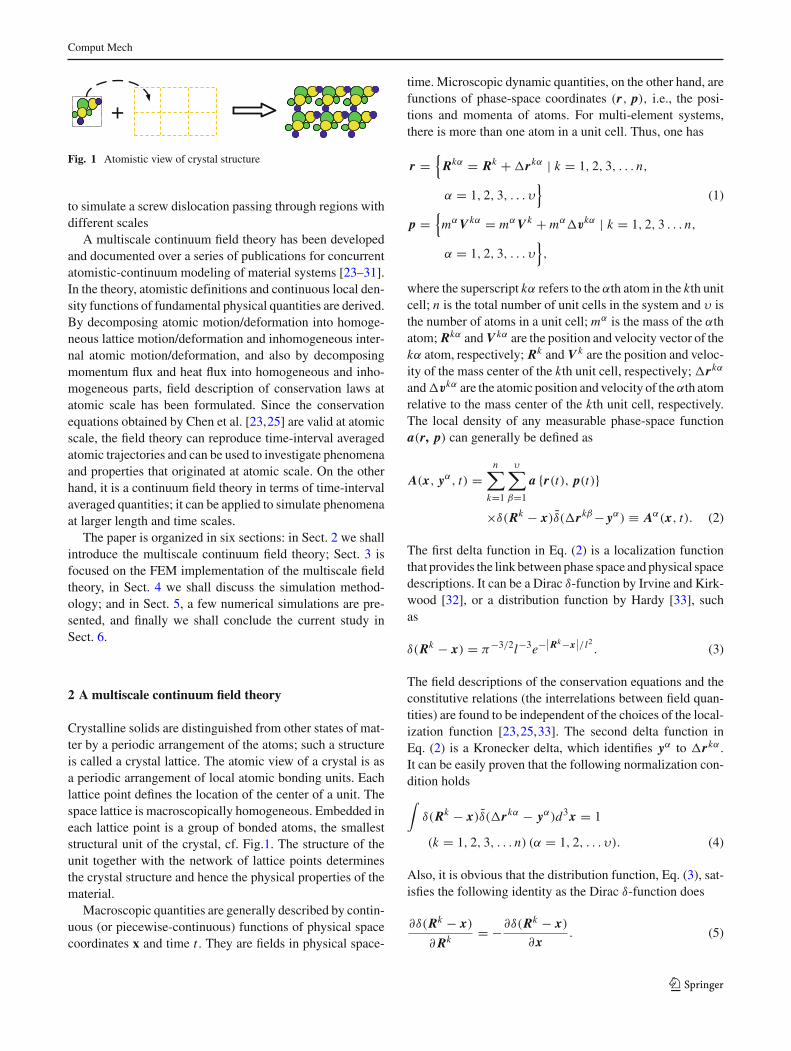
Fig. 1 Atomistic view of crystal structure

to simulate a screw dislocation passing through regions withdifferent scales

A multiscale continuum field theory has been developedand documented over a series of publications for concurrentatomistic-continuum modeling of material systems [23–31].In the theory, atomistic definitions and continuous local den-sity functions of fundamental physical quantities are derived.By decomposing atomic motion/deformation into homoge-neous lattice motion/deformation and inhomogeneous inter-nal atomic motion/deformation, and also by decomposingmomentum flux and heat flux into homogeneous and inho-mogeneous parts, field description of conservation laws atatomic scale has been formulated. Since the conservationequations obtained by Chen et al. [23,25] are valid at atomicscale, the field theory can reproduce time-interval averagedatomic trajectories and can be used to investigate phenomenaand properties that originated at atomic scale. On the otherhand, it is a continuum field theory in terms of time-intervalaveraged quantities; it can be applied to simulate phenomenaat larger length and time scales.

The paper is organized in six sections: in Sect. 2 we shallintroduce the multiscale continuum field theory; Sect. 3 isfocused on the FEM implementation of the multiscale fieldtheory, in Sect. 4 we shall discuss the simulation method-ology; and in Sect. 5, a few numerical simulations are pre-sented, and finally we shall conclude the current study inSect. 6.

2 A multiscale continuum field theory

Crystalline solids are distinguished from other states of mat-ter by a periodic arrangement of the atoms; such a structureis called a crystal lattice. The atomic view of a crystal is asa periodic arrangement of local atomic bonding units. Eachlattice point defines the location of the center of a unit. Thespace lattice is macroscopically homogeneous. Embedded ineach lattice point is a group of bonded atoms, the smalleststructural unit of the crystal, cf. Fig.1. The structure of theunit together with the network of lattice points determinesthe crystal structure and hence the physical properties of thematerial.

Macroscopic quantities are generally described by contin-uous (or piecewise-continuous) functions of physical spacecoordinates x and time t. They are fields in physical space-

time. Microscopic dynamic quantities, on the other hand, arefunctions of phase-space coordinates (r, p), i.e., the posi-tions and momenta of atoms. For multi-element systems,there is more than one atom in a unit cell. Thus, one has

r ={

Rkα = Rk + �rkα | k = 1, 2, 3, . . . n,

α = 1, 2, 3, . . . υ}

(1)

p ={

mαV kα = mαV k + mα�vkα | k = 1, 2, 3 . . . n,

α = 1, 2, 3, . . . υ},

where the superscript kα refers to the αth atom in the kth unitcell; n is the total number of unit cells in the system and υ isthe number of atoms in a unit cell; mα is the mass of the αthatom; Rkα and V kα are the position and velocity vector of thekα atom, respectively; Rk and V k are the position and veloc-ity of the mass center of the kth unit cell, respectively; �rkα

and �vkα are the atomic position and velocity of the αth atomrelative to the mass center of the kth unit cell, respectively.The local density of any measurable phase-space functiona(r, p) can generally be defined as

A(x, yα, t) =n∑

k=1

υ∑β=1

a {r(t), p(t)}

×δ(Rk − x)δ(�rkβ − yα) ≡ Aα(x, t). (2)

The first delta function in Eq. (2) is a localization functionthat provides the link between phase space and physical spacedescriptions. It can be a Dirac δ-function by Irvine and Kirk-wood [32], or a distribution function by Hardy [33], suchas

δ(Rk − x) = π−3/2l−3e−∣∣Rk−x∣∣/ l2

. (3)

The field descriptions of the conservation equations and theconstitutive relations (the interrelations between field quan-tities) are found to be independent of the choices of the local-ization function [23,25,33]. The second delta function inEq. (2) is a Kronecker delta, which identifies yα to �rkα.

It can be easily proven that the following normalization con-dition holds∫

δ(Rk − x)δ(�rkα − yα)d3x = 1

(k = 1, 2, 3, . . . n) (α = 1, 2, . . . υ). (4)

Also, it is obvious that the distribution function, Eq. (3), sat-isfies the following identity as the Dirac δ-function does

∂δ(Rk − x)

∂ Rk= −∂δ(Rk − x)

∂x. (5)

123

Comput Mech

Physical properties, such as thermodynamic properties andtransport properties, refer only to average behavior. In thepast, this was achieved through the theory of statisticalmechanics. Averages were constructed by including manysimilar systems with different initial conditions. By this pro-cedure, starting the system in any initial configuration wouldyield the same average quantities: this explains the reproduc-ibility of experiments. Therefore, in statistical mechanics, amacroscopic field quantity is defined as the ensemble averageof an instantaneous dynamical function. Most current MDapplications involve systems which are either in equilibriumor in some time-independent stationary state; where individ-ual results are subjected to fluctuation; it is the well-definedaverages over sufficiently long time intervals that are of inter-est. To smooth out the results and to obtain results close toexperiments, measurements of physical quantities are neces-sary to be collected and averaged over finite time duration.Therefore, in deriving the field description of atomic quan-tities and balance equations, it is the time-interval averagedquantities that are involved. The time-interval averaged (attime t in the interval [t, t + �t]) local density function isdefined as

Aα(x, t) = ⟨

Aα(x, t)⟩ ≡ 1

�t

�t∫

0

Aα(x, t + τ)dτ

= 1

�t

�t∫

0

n∑k=1

a{r(t + τ), p(t + τ)}

×δ(Rk − x)δ(�rkα − yα)dτ. (6)

With the help of Eq. (5), the time evolution of the local den-sity function can be obtained as

∂ Aα

∂t

∣∣∣x, yα

=n∑

k=1

dadt

δ(Rk − x)δ(�rkα − yα)

−∇x ·[

n∑k=1

V k ⊗ aδ(Rk − x)δ(�rkα − yα)

]

−∇ yα ·[

n∑k=1

�vkα ⊗ aδ(Rk − x)δ(�rkα − yα)

].

(7)

When Aα is a conserved property, it results in a local con-servation law that governs the time evolution of Aα. Themathematical representation of conservation equations formass, linear momentum and energy at atomic scale has beenanalytically obtained in terms of averaged field quantities

[23,25,30], which are

dρα

dt+ ρα∇x · v + ρα∇yα · �vα = 0 (8)

ρα d

dt(v + �vα) = ∇x · tα + ∇yα · τα + ϕα (9)

ρα deα

dt+ ∇x · (−qα) + ∇yα · (− j

α)

= tα : ∇x(v + �vα) + τα : ∇yα (v + �vα) + hα (10)

where the time-interval averaged mass density ρα, linearmomentum ρα(v + �vα), homogeneous atomic stressestα(kin) + tα(pot) and inhomogeneous atomic stresses τα

(kin) +τα

(pot), body force density ϕα, internal energy density ρα eα,

the homogeneous part qα and inhomogeneous part jα

of heatflux, and heat source hα are defined as

ρα(x, t) ≡⟨

n∑k=1

mαδ(Rk − x)δ(�rkα − yα)

⟩, (11)

ρα(v + �vα) ≡⟨

n∑k=1

mα(V k + �vkα)δ(Rk − x)

× δ(�rkα − yα)

⟩, (12)

tα(kin) ≡ −⟨

n∑k=1

mα Vk ⊗ V

kαδ(Rk − x)

× δ(�rkα − yα)

⟩, (13)

τα(kin) ≡ −

⟨n∑

k=1

mα�vkα ⊗ Vkα

δ(Rk − x)

× δ(�rkα − yα)

⟩, (14)

tα(pot) ≡ −1

2

⟨n∑

k,l=1

υ∑ξ,η=1

(Rk − Rl)

⊗Fkξ B(k, ξ, l, η, x, yα)

⟩, (15)

τα(pot) ≡ −1

2

⟨n∑

k,l=1

υ∑ξ,η=1

(�rkξ − �rlη)

⊗Fkξ B(k, ξ, l, η, x, yα)

⟩, (16)

ϕα ≡⟨

n∑k=1

ϕkαδ(Rk − x) × δ(�rkα − yα)

⟩, (17)

123

Comput Mech

ρα eα ≡⟨ Nl∑

k=1

Na∑ξ=1

[1

2mξ (V

kξ)2 + U kξ

]δ(Rk − x)

× δ(�rkξ − yα)

⟩, (18)

qαkin ≡ −

⟨ Nl∑k=1

Na∑ξ=1

Vk(

1

2mξ (V

kξ)2 + U kξ

)

× δ(Rk − x)δ(�rkξ − yα)

⟩, (19)

qαpot ≡ −

⟨1

2

Nl∑k,l=1

Na∑ξ,η=1

(Rk − Rl)Vkξ

·Fkξ B(k, ξ, l, η, x, yα)

⟩, (20)

jα

kin ≡ −⟨ Nl∑

k=1

Na∑ξ=1

�vkξ

(1

2mξ (V

kξ)2 + U kξ

)

× δ(Rk − x)δ(�rkξ − yα)

⟩, (21)

jα

pot ≡ −⟨

1

2

Nl∑k,l=1

Na∑ξ,η=1

(�rkξ−�rlη)Vkξ

·Fkξ B(k, ξ, l, η, x, yα)

⟩, (22)

hα ≡⟨ Nl∑

k=1

Na∑ξ=1

Vkξ · ϕkξ δ(Rk − x)

× δ(�rkξ − yα)

⟩, (23)

where Fkξ is the interatomic force acting on the kξ atom;ϕkα is the body force acting the kα atom; U kξ is the potentialenergy of the kξ atom;

Vkα ≡ V kα − v − �vα, V

k ≡ V k − v,

�vkα ≡ �vkα − �vα, (24)

B(k, ξ, l, η, x, yα) ≡1∫

0

dλδ(

Rkλ + Rl(1 − λ) − x)

× δ(�rkξ λ + �r

lη(1 − λ) − yα

).

(25)

where v is the time interval averaged velocity of the centroidof a unit cell and �vα is the time interval averaged velocityof the αth atom relative to the centroid of the unit cell.

It is worthwhile to note that, with the atomistic definitionsof interatomic force and the potential parts of the atomicstresses, one has

∇x · tα(pot) + ∇yα · τα(pot) = f

α, (26)

where fα

is the interatomic force density acting on the αthatom in the unit cell located at x .

3 Finite element formulation

In the finite element formulation, we work with time-intervalaveraged quantities. From now on, for simplicity, we adoptthe following abbreviations:

uα ≡ d(v + �vα)

dt, tα(kin) ≡ tα, τα

(kin) ≡ τα,

fα ≡ f α/V, ϕα ≡ ϕα/V, (27)

where uα is the displacement vector of the αth atom; V isthe volume of unit cell. The governing equation, Eq. (9), cannow be rewritten as

mα uα = {∇x · tα + ∇ yα · τα}

V + f α + ϕα. (28)

For single-element atomic system, Cheung and Yip [34] andHaile [35] gave the definitions for kinetic stresses ti j andtemperature T . In consistent with their definitions, for multi-element atomic system, we have

tαi j = −〈mαvi (v j + �vαj )〉/V, (29)

ταi j = −〈mα�vα

i (v j + �vαj )〉/V, (30)

3kB T α = 〈mα(vi + �vαi )(vi + �vα

i )〉. (31)

At high temperature and within harmonic approximation, allmodes have the same energy [43]. Following this thinking,we take the assumption, made by Xiong et al. [27], whichrelates the energies of acoustic modes and optic modes andwe further assume that the temperature within a unit cell isuniform. This implies T α = T (x, t) and ∇yα · τα = 0. Nowthe governing equation, Eq. (28), can be rewritten as

mα uα = V ∇ · tα + f α + ϕα, (32)

with tαi j = −γ αkB T δi j/V, ταi j = −(1 − γ α)kB T δi j/V and

γ α ≡ mα/∑ν

α=1 mα. In this work, we are only concernedwith ‘one-way coupling’ with temperature and electromag-netic fields, i.e., the temperature and electromagnetic fieldsare given as functions of space and time. Then the rele-vant governing equations are just the balance law for linearmomentum:

mα uα = −γ αkB∇T + f α + ϕα. (33)

In case of temperature being constant, including T = 0, wecan drop the first term in the right hand side of Eq. (33), and

123

Comput Mech

the governing equation for any αth atom in the kth unit cellcan be rewritten as

mα u(k, α) = f (k, α) + ϕ(k, α), (34)

where f (k, α) is all the interatomic force acting on the αthatom in the kth unit cell; ϕ(k, α) is all the body force dueto external field acting on the αth atom in the kth unit cell.The effect of non zero temperature should be reflected inthe boundary conditions. However, in this work we considerzero-temperature. Therefore, for a system with pair potential,one may rewrite Eq. (34) as

mα u(k, α) =n∑

l=1

υ∑β=1

f (k, α; l, β) + ϕ(k, α), (35)

where f (k, α; l, β) is the interatomic force acting on the αthatom of the kth unit cell due to the interaction with the βthatom of the lth unit cell, with the understanding (k, α) �=(l, β). The inner product of Eq. (35) with virtual displace-ment δu(k, α) leads to

mα u(k, α) · δu(k, α)

=n∑

l=1

υ∑β=1

f (k, α; l, β) · δu(k, α) + ϕ(k, α) · δu(k, α).

(36)

Sum over all α and k, we obtain the following variationalequation, the so-called weak form, as

n∑k=1

υ∑α=1

mα u(k, α) · δu(k, α)

=n∑

k=1

υ∑α=1

⎧⎨⎩

n∑l=1

υ∑β=1

f (k, α; l, β) + ϕ(k, α)

⎫⎬⎭ · δu(k, α).

(37)

Notice that Eq. (37) can also be expressed as

n∑k=1

υ∑α=1

mα u(k, α) · δu(k, α)

=n∑

k=1

υ∑α=1

n∑l=1

υ∑β=1

f (l, β; k, α) · δu(l, β)

+n∑

k=1

υ∑α=1

ϕ(k, α) · δu(k, α). (38)

It is noticed that

f (k, α; l, β) = − f (l, β; k, α), (39)

Therefore Eq. (38) can be rewritten as

n∑k=1

υ∑α=1

mα u(k, α) · δu(k, α)

= 1

2

n∑k=1

υ∑α=1

n∑l=1

υ∑β=1

f (k, α; l, β) · [δu(k, α) − δu(l, β)]

+n∑

k=1

υ∑α=1

ϕ(k, α) · δu(k, α). (40)

Suppose the whole specimen is divided into Ne finite ele-ments (8-node solid elements) with Np finite elements nodes,and we approximate Eq. (40) as [30]

Np∑Ip=1

υ∑α=1

V (Ip)

V

⎧⎨⎩mα u(Ip, α) · δu(Ip, α)−ϕ(Ip, α) · δu(Ip, α)

−1

2

n∑l=1

υ∑β=1

f (Ip, α; l, β) · [δu(Ip, α) − δu(l, β)]⎫⎬⎭ = 0,

(41)

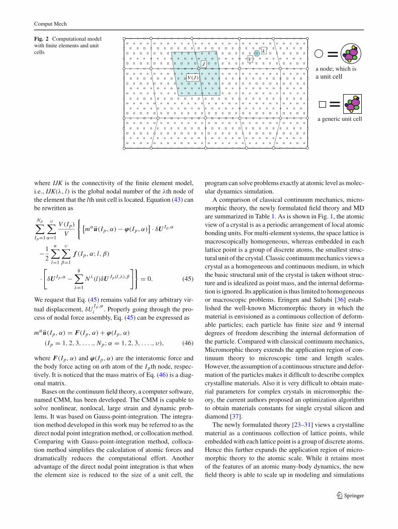
where V (Ip) is the volume associated with the Ipth nodeand V is the volume of a unit cell; f (Ip, α; l, β) is the forceacting on the αth atom of the Ipth finite element node dueto the interaction with the βth atom of the lth unit cell. Forthe purpose of illustration, a 2D schematic picture shows thecomputational model with finite elements in Fig. 2, in whichthe large shaded area (volume) V (J ) around the J th nodemeans the area (volume) associated with the J th node andthe small shaded area (volume) V around the kth unit cellmeans the area (volume) associated with the kth unit cell.

Through the shape functions, one may have

δu(l, β) =8∑

λ=1

Nλ(l)δUβ(l, λ), (42)

where Nλ(l) is the λth shape function evaluated at the centerof the lth unit cell; δUβ(l, λ) is the virtual displacement ofthe βth atom of λth node of the element where the lth unitcell is located.

Now one may rewrite Eq. (41) as

Np∑Ip=1

υ∑α=1

V (Ip)

V

{mα u(Ip, α) · δu(Ip, α) − ϕ(Ip, α)

·δu(Ip, α) − 1

2

n∑l=1

υ∑β=1

f (Ip, α; l, β)

·[δu(Ip, α) −

8∑λ=1

Nλ(l)δUβ(l, λ)

]}= 0. (43)

Let

Jp(l, λ) ≡ IJK(λ, l), (44)

123

Comput Mech

Fig. 2 Computational modelwith finite elements and unitcells

a node; which is a unit cell

a generic unit cell

k

V

( )V J

J

where IJK is the connectivity of the finite element model,i.e., IJK(λ, l) is the global nodal number of the λth node ofthe element that the lth unit cell is located. Equation (43) canbe rewritten as

Np∑Ip=1

υ∑α=1

V (Ip)

V

{ [mα u(Ip, α) − ϕ(Ip, α)

] · δU Ip,α

−1

2

n∑l=1

υ∑β=1

f (Ip, α; l, β)

·[δU Ip,α −

8∑λ=1

Nλ(l)δU Jp(l,λ),β

]}= 0. (45)

We request that Eq. (45) remains valid for any arbitrary vir-

tual displacement, δUIp,α

i . Properly going through the pro-cess of nodal force assembly, Eq. (45) can be expressed as

mα u(Ip, α) = F(Ip, α) + ϕ(Ip, α)

(Ip = 1, 2, 3, . . . ., Np;α = 1, 2, 3, . . . ., υ), (46)

where F(Ip, α) and ϕ(Ip, α) are the interatomic force andthe body force acting on αth atom of the Ipth node, respec-tively. It is noticed that the mass matrix of Eq. (46) is a diag-onal matrix.

Bases on the continuum field theory, a computer software,named CMM, has been developed. The CMM is capable tosolve nonlinear, nonlocal, large strain and dynamic prob-lems. It was based on Gauss-point-integration. The integra-tion method developed in this work may be referred to as thedirect nodal point integration method, or collocation method.Comparing with Gauss-point-integration method, colloca-tion method simplifies the calculation of atomic forces anddramatically reduces the computational effort. Anotheradvantage of the direct nodal point integration is that whenthe element size is reduced to the size of a unit cell, the

program can solve problems exactly at atomic level as molec-ular dynamics simulation.

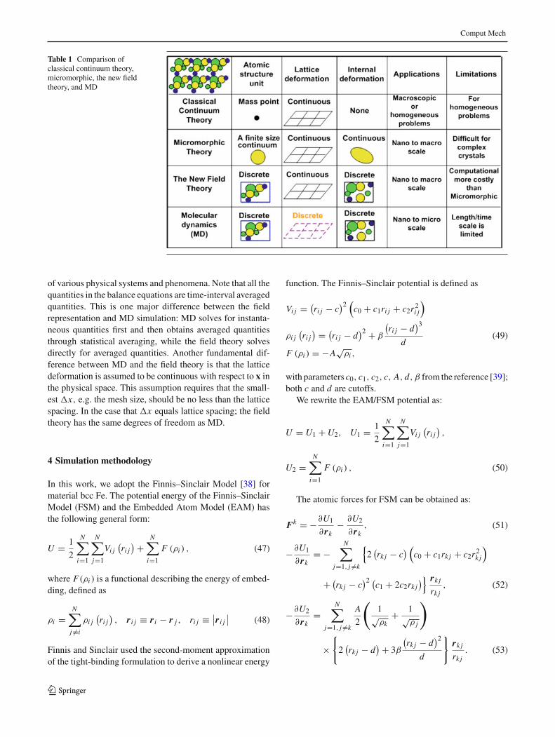
A comparison of classical continuum mechanics, micro-morphic theory, the newly formulated field theory and MDare summarized in Table 1. As is shown in Fig. 1, the atomicview of a crystal is as a periodic arrangement of local atomicbonding units. For multi-element systems, the space lattice ismacroscopically homogeneous, whereas embedded in eachlattice point is a group of discrete atoms, the smallest struc-tural unit of the crystal. Classic continuum mechanics views acrystal as a homogeneous and continuous medium, in whichthe basic structural unit of the crystal is taken without struc-ture and is idealized as point mass, and the internal deforma-tion is ignored. Its application is thus limited to homogeneousor macroscopic problems. Eringen and Suhubi [36] estab-lished the well-known Micromorphic theory in which thematerial is envisioned as a continuous collection of deform-able particles; each particle has finite size and 9 internaldegrees of freedom describing the internal deformation ofthe particle. Compared with classical continuum mechanics,Micromorphic theory extends the application region of con-tinuum theory to microscopic time and length scales.However, the assumption of a continuous structure and defor-mation of the particles makes it difficult to describe complexcrystalline materials. Also it is very difficult to obtain mate-rial parameters for complex crystals in micromorphic the-ory, the current authors proposed an optimization algorithmto obtain materials constants for single crystal silicon anddiamond [37].

The newly formulated theory [23–31] views a crystallinematerial as a continuous collection of lattice points, whileembedded with each lattice point is a group of discrete atoms.Hence this further expands the application region of micro-morphic theory to the atomic scale. While it retains mostof the features of an atomic many-body dynamics, the newfield theory is able to scale up in modeling and simulations

123

Comput Mech

Table 1 Comparison ofclassical continuum theory,micromorphic, the new fieldtheory, and MD

of various physical systems and phenomena. Note that all thequantities in the balance equations are time-interval averagedquantities. This is one major difference between the fieldrepresentation and MD simulation: MD solves for instanta-neous quantities first and then obtains averaged quantitiesthrough statistical averaging, while the field theory solvesdirectly for averaged quantities. Another fundamental dif-ference between MD and the field theory is that the latticedeformation is assumed to be continuous with respect to x inthe physical space. This assumption requires that the small-est �x, e.g. the mesh size, should be no less than the latticespacing. In the case that �x equals lattice spacing; the fieldtheory has the same degrees of freedom as MD.

4 Simulation methodology

In this work, we adopt the Finnis–Sinclair Model [38] formaterial bcc Fe. The potential energy of the Finnis–SinclairModel (FSM) and the Embedded Atom Model (EAM) hasthe following general form:

U = 1

2

N∑i=1

N∑j=1

Vi j(ri j

) +N∑

i=1

F (ρi ) , (47)

where F(ρi ) is a functional describing the energy of embed-ding, defined as

ρi =N∑

j �=i

ρi j(ri j

), r i j ≡ r i − r j , ri j ≡ ∣∣r i j

∣∣ (48)

Finnis and Sinclair used the second-moment approximationof the tight-binding formulation to derive a nonlinear energy

function. The Finnis–Sinclair potential is defined as

Vi j = (ri j − c

)2(

c0 + c1ri j + c2r2i j

)

ρi j(ri j

) = (ri j − d

)2 + β

(ri j − d

)3

d(49)

F (ρi ) = −A√

ρi ,

with parameters c0, c1, c2, c, A, d, β from the reference [39];both c and d are cutoffs.

We rewrite the EAM/FSM potential as:

U = U1 + U2, U1 = 1

2

N∑i=1

N∑j=1

Vi j(ri j

),

U2 =N∑

i=1

F (ρi ) , (50)

The atomic forces for FSM can be obtained as:

Fk = −∂U1

∂ rk− ∂U2

∂ rk, (51)

−∂U1

∂ rk= −

N∑j=1, j �=k

{2(rk j − c

) (c0 + c1rk j + c2r2

k j

)

+ (rk j − c

)2 (c1 + 2c2rk j

)} rk j

rk j, (52)

−∂U2

∂ rk=

N∑j=1, j �=k

A

2

(1√ρk

+ 1√ρ j

)

×{

2(rk j − d

) + 3β

(rk j − d

)2

d

}rk j

rk j. (53)

123

Comput Mech

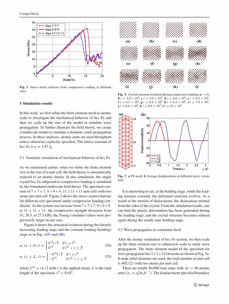
Fig. 3 Stress–strain relations from compressive loading at differentsizes

5 Simulation results

In this work, we first refine the finite element mesh to atomicscale to investigate the mechanical behavior of bcc Fe andthen we scale up the size of the model to simulate wavepropagation. To further illustrate the field theory, we createa multiscale model to simulate a dynamic crack propagationprocess. In these analyses, atomic units are used throughoutunless otherwise explicitly specified. The lattice constant ofbcc Fe is a = 2.87 Å .

5.1 Atomistic simulation of mechanical behavior of bcc Fe

As we mentioned earlier, when we refine the finite elementsize to the size of a unit cell, the field theory is automaticallyreduced to an atomic theory. In this simulation, the singlecrystal bcc Fe subjected to compressive loading is simulatedby the formulated multiscale field theory. The specimen con-sists of 7×7×7, 9×9×9, 11×11×11 unit cells with twoatoms per unit cell. Figure 3 shows the stress–strain relationsfor different size specimens under compressive loading con-ditions. As the system size increase from 7×7×7, 9×9×9,

to 11 × 11 × 11, the compressive strength decreases from31, 29.5, to 27.5 GPa, the Young’s modules values were pro-gressively larger in our case.

Figure 4 shows the structural evolution during the linearlyincreasing loading stage and the constant loading (holding)stage as in Eqs. (45) and (46).

uz (x, y, 0, t) ={

U 0t/T if t ≤ t0

U 0 if t0 < t ≤ T(54)

uz (x, y, L , t) ={−U 0t/T if t ≤ t0

−U 0 if t0 < t ≤ T(55)

where U 0 = εL/2 with ε is the applied strain, L is the totallength of the specimen, t0 = 0.6T .

Fig. 4 Crystal structure evolution during compressive loading: a t = 0,b t = 2.0 × 105, c t = 4.0 × 105, d t = 6.0 × 105, e t = 6.2 × 105,f t = 6.3 × 105, g t = 6.4 × 105, h t = 6.5 × 105, i t = 7.0 × 105,j t = 8.0 × 105, k t = 9.0 × 105, l t = 10 × 105

Fig. 5 a FE mesh. b Average displacements at different layers versustime

It is interesting to see, at the holding stage, while the load-ing remains constant, the deformed structure evolves. As aresult of the motion of dislocations, the dislocation emittedfrom the sides of the crystal. From the simulation results, onecan find the plastic deformation has been generated duringthe loading stage, and the crystal structure becomes orderedagain during the steady state holding stage.

5.2 Wave propagation at continuum level

After the atomic simulation of bcc Fe system, we then scaleup the finite element size to submicron scale to study wavepropagation. The finite element model of the specimen forwave propagation has 2×2×12 elements as shown in Fig. 5a.8-node solid elements are used; the total number of unit cellis 405,121 with two atoms per unit cell.

There are totally 80,000 time steps with �t = 40 atomicunits (τo ≡ a2

omeh−1). The displacement specified boundary

123

Comput Mech

conditions are applied at the two ends of the specimen as

uz (x, y, 0, t) ={

U 0 sin ωt if t ≤ t0

0 if t0 < t ≤ T, (56)

uz (x, y, L , t) = 0, (57)

where U 0 = εL with ε = 0.02;ω = π/to with t0 = T/4;the total length of the specimen is L ≈ 69.2 nm; the totalsimulation time is T = 3,200,000 τo ≈ 77.5 ps. The phe-nomenon of wave propagation has been observed in the simu-lation. Figure 5b shows the displacements at different layersof the specimen, the top surface of the specimen is fixed,the half-sine wave is generated at the bottom surface and wecaptured the wave at the central layer of the specimen. Basedon the simulation results, the wave speed of the travelingwave in the bcc iron is estimated to be 4770 m/s, which isin reasonable agreement with the experimental value aroundvL = √

C11/ρ = 5326 m/s [40]. The predicted wave speedis lower than the experimental value. The possible reason isthat maybe the potential we are using is not good enough.

5.3 Multiscale modeling and simulation of dynamic crackpropagation

The traditional continuum-based theories of fracture mechan-ics provide the basic computational and modeling tools forstudying the fracture processes. These theories provide a vari-ety of energy and stress criteria for computing the conditionsfor further growth of a static crack on the verge of extension.Despite their valuable contributions, a modeling of a fractureprocess based exclusively on these theories is not, however,capable of accounting for all of the experimentally observedcharacteristics of the crack dynamics or the crack-surfacetopography. These microscopic properties of materials areoften determined by events on the atomic scale. So, for thedetailed understanding of fracture and crack propagation, werequire an understanding in the atomic scale. But atomisticstudies of fracture are computationally rather demanding.Again, in the region away from the crack-tip we do not needthe atomic scale discretization. This leads to the use of a mul-tiscale modeling approach that couples the crack propagationacross several length scales within one unified and seamlessmodel, which would be able to provide deeper insights intothe peculiarities of the crack dynamics.

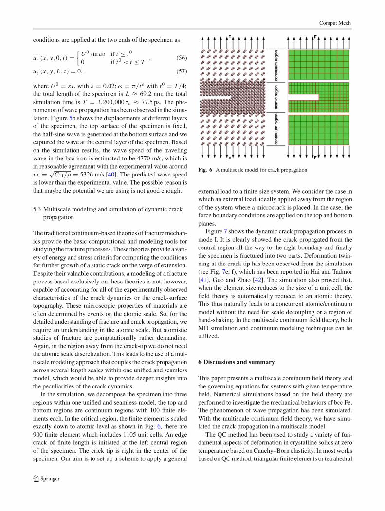
In the simulation, we decompose the specimen into threeregions within one unified and seamless model, the top andbottom regions are continuum regions with 100 finite ele-ments each. In the critical region, the finite element is scaledexactly down to atomic level as shown in Fig. 6, there are900 finite element which includes 1105 unit cells. An edgecrack of finite length is initiated at the left central regionof the specimen. The crick tip is right in the center of thespecimen. Our aim is to set up a scheme to apply a general

Fig. 6 A multiscale model for crack propagation

external load to a finite-size system. We consider the case inwhich an external load, ideally applied away from the regionof the system where a microcrack is placed. In the case, theforce boundary conditions are applied on the top and bottomplanes.

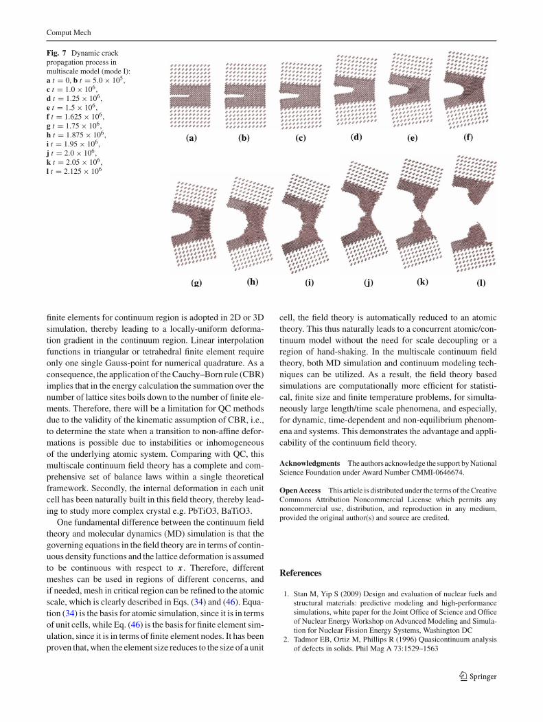
Figure 7 shows the dynamic crack propagation process inmode I. It is clearly showed the crack propagated from thecentral region all the way to the right boundary and finallythe specimen is fractured into two parts. Deformation twin-ning at the crack tip has been observed from the simulation(see Fig. 7e, f), which has been reported in Hai and Tadmor[41], Guo and Zhao [42]. The simulation also proved that,when the element size reduces to the size of a unit cell, thefield theory is automatically reduced to an atomic theory.This thus naturally leads to a concurrent atomic/continuummodel without the need for scale decoupling or a region ofhand-shaking. In the multiscale continuum field theory, bothMD simulation and continuum modeling techniques can beutilized.

6 Discussions and summary

This paper presents a multiscale continuum field theory andthe governing equations for systems with given temperaturefield. Numerical simulations based on the field theory areperformed to investigate the mechanical behaviors of bcc Fe.The phenomenon of wave propagation has been simulated.With the multiscale continuum field theory, we have simu-lated the crack propagation in a multiscale model.

The QC method has been used to study a variety of fun-damental aspects of deformation in crystalline solids at zerotemperature based on Cauchy–Born elasticity. In most worksbased on QC method, triangular finite elements or tetrahedral

123

Comput Mech

Fig. 7 Dynamic crackpropagation process inmultiscale model (mode I):a t = 0, b t = 5.0 × 105,c t = 1.0 × 106,d t = 1.25 × 106,e t = 1.5 × 106,f t = 1.625 × 106,g t = 1.75 × 106,h t = 1.875 × 106,i t = 1.95 × 106,j t = 2.0 × 106,k t = 2.05 × 106,l t = 2.125 × 106

finite elements for continuum region is adopted in 2D or 3Dsimulation, thereby leading to a locally-uniform deforma-tion gradient in the continuum region. Linear interpolationfunctions in triangular or tetrahedral finite element requireonly one single Gauss-point for numerical quadrature. As aconsequence, the application of the Cauchy–Born rule (CBR)implies that in the energy calculation the summation over thenumber of lattice sites boils down to the number of finite ele-ments. Therefore, there will be a limitation for QC methodsdue to the validity of the kinematic assumption of CBR, i.e.,to determine the state when a transition to non-affine defor-mations is possible due to instabilities or inhomogeneousof the underlying atomic system. Comparing with QC, thismultiscale continuum field theory has a complete and com-prehensive set of balance laws within a single theoreticalframework. Secondly, the internal deformation in each unitcell has been naturally built in this field theory, thereby lead-ing to study more complex crystal e.g. PbTiO3, BaTiO3.

One fundamental difference between the continuum fieldtheory and molecular dynamics (MD) simulation is that thegoverning equations in the field theory are in terms of contin-uous density functions and the lattice deformation is assumedto be continuous with respect to x. Therefore, differentmeshes can be used in regions of different concerns, andif needed, mesh in critical region can be refined to the atomicscale, which is clearly described in Eqs. (34) and (46). Equa-tion (34) is the basis for atomic simulation, since it is in termsof unit cells, while Eq. (46) is the basis for finite element sim-ulation, since it is in terms of finite element nodes. It has beenproven that, when the element size reduces to the size of a unit

cell, the field theory is automatically reduced to an atomictheory. This thus naturally leads to a concurrent atomic/con-tinuum model without the need for scale decoupling or aregion of hand-shaking. In the multiscale continuum fieldtheory, both MD simulation and continuum modeling tech-niques can be utilized. As a result, the field theory basedsimulations are computationally more efficient for statisti-cal, finite size and finite temperature problems, for simulta-neously large length/time scale phenomena, and especially,for dynamic, time-dependent and non-equilibrium phenom-ena and systems. This demonstrates the advantage and appli-cability of the continuum field theory.

Acknowledgments The authors acknowledge the support by NationalScience Foundation under Award Number CMMI-0646674.

Open Access This article is distributed under the terms of the CreativeCommons Attribution Noncommercial License which permits anynoncommercial use, distribution, and reproduction in any medium,provided the original author(s) and source are credited.

References

1. Stan M, Yip S (2009) Design and evaluation of nuclear fuels andstructural materials: predictive modeling and high-performancesimulations, white paper for the Joint Office of Science and Officeof Nuclear Energy Workshop on Advanced Modeling and Simula-tion for Nuclear Fission Energy Systems, Washington DC

2. Tadmor EB, Ortiz M, Phillips R (1996) Quasicontinuum analysisof defects in solids. Phil Mag A 73:1529–1563

123

Comput Mech

3. Ericksen JL (1984) The Cauchy and born hypothesis for crystals.In: Gurtin M (ed) Phase transformations and material instabilitiesin solids. Academic Press, New York, pp 61–77

4. Rudd RE, Broughton JQ (1998) Coarse-grained molecular dynam-ics and atomic limit of finite elements. Phys Rev B 58:5893–5896

5. Rudd RE, Broughton JQ (2000) Concurrent coupling of lengthscales in solid state systems. Phys Stat Sol 217:251–291

6. Abraham F, Broughton J, Bernstein N, Kaxiras E (1998) Spanningthe length scales in dynamic simulation. Comput Phys 12:538–546

7. Broughton J, Bernstein N, Kaxiras E, Abraham F (1999) Concur-rent coupling of length scales: methodology and application. PhysRev B 60:2391–2403

8. Rudd RE, Broughton JQ (1999) Atomistic simulation of MEMSresonators trough the coupling of length scales. J Model SimulMicrosyst 1(1):29–38

9. Li XT, E W (2005) Multiscale modeling of dynamics of solids atfinite temperature. J Mech Phys Solids 53:1650–1685

10. E W, Engquist B (2003) The heterogeneous multi-scale methods.Comm Math Sci 1(1):87–132

11. Wagner GJ, Karpov EG, Liu WK (2004) Molecular dynamicsboundary conditions for regular crystal lattices. Comput MethodsAppl Mech Eng 193(17–20):1579–1601

12. Qian D, Wagner GJ, Liu WK (2004) A multiscale projectionmethod for the analysis of carbon nanotubes. Comput MethodsAppl Mech Eng 193:1603–1632

13. Wagner GJ, Liu WK (2003) Coupling of atomic and continuumsimulations using a bridging scale decomposition. J Comput Phys190:249–274

14. Karpov EG, Yu H, Park H, Liu WK, Wang J, Qian D (2006) Mul-tiscale boundary conditions in crystalline solids: theory and appli-cation to nanoindentation. Int J Solids Struct 43(21):6359–6379

15. Park HS, Karpov EG, Liu WK, Klein PA (2005) The bridgingscale for three-dimensional atomistic/continuum coupling. PhilMag 85(1):79–113

16. Xiao SP, Belytschko T (2004) A bridging domain method for cou-pling continua with molecular dynamics. Comput Methods ApplMech Eng 193:1645–1669

17. Vernerey FJ, Liu WK, Moran B (2007) Multi-scale micromorphictheory for hierarchical materials. J Mech Phys Solid 55(12):2603–2651

18. Vernerey FJ, Liu WK, Moran B, Olson GB (2008) A micromorphicmodel for the multiple scale failure of heterogeneous materials.J Mech Phys Solids 56(4):1320–1347

19. McVeigh C, Liu WK (2008) Linking microstructure and propertiesthrough a predictive multiresolution continuum. Comput MethodsAppl Mech Eng 197:3268–3290

20. McVeigh C, Liu WK (2009) Multiresolution modeling of ductilereinforced brittle composites. J Mech Phys Solids 57:244–267

21. To AC, Li S (2005) Perfectly matched multiscale simulations. PhysRev B 72:035414

22. Li S, Liu X, Agrawal A, To AC (2006) Perfectly matched multi-scale simulations for discrete systems: extension to multiple dimen-sions. Phys Rev B 74:045418

23. Chen Y, Lee JD (2005) Atomistic formulation of a multiscale the-ory for nano/micro physics. Phil Mag 85:4095–4126

24. Chen Y (2006) Local stress and heat flux in atomistic systemsinvolving three-body forces. J Chem Phys 124:054113

25. Chen Y, Lee JD (2006) Conservation laws at nano/micro scales.J Mech Mater Struct 1:681–704

26. Chen Y, Lee JD, Xiong L (2006) Stresses and strains at nano/microscales. J Mech Mater Struct 1:705–723

27. Xiong L, Chen Y, Lee JD (2007) Atomistic simulation of mechan-ical properties of diamond and silicon by a field theory. ModelSimul Mater Sci Eng 15:535–551

28. Lei Y, Lee JD, Zeng X (2008) Response of a rocksalt crystal toelectromagnetic wave modeled by a multiscale field theory. Inter-act Multiscale Mech 1(4):467–476

29. Chen Y (2009) Reformulation of microscopic balance equationsfor multiscale materials modeling. J Chem Phys 130(13):134706

30. Lee JD, Wang XQ, Chen Y (2009) Multiscale material modelingand its application to a dynamic crack propagation problem. TheorAppl Fracture Mech 51:33–40

31. Lee JD, Wang XQ, Chen Y (2009) Multiscale computational fornano/micro material. J Eng Mech 135:192–202

32. Irvine JH, Kirkwood JG (1950) The statistical theory of trans-port processes. IV. The equations of hydrodynamics. J Chem Phys18:817

33. Hardy RJ (1982) Formulas for determining local properties inmolecular-dynamics simulations: shock waves. J Chem Phys76(1):622–628

34. Cheung KS, Yip S (1991) Atomic-level stress in an inhomoge-neous system. J Appl Phys 70(10):5688–5690

35. Haile JM (1992) Molecular dynamics simulation. Wiley, New York36. Eringen AC, Suhubi ES (1964) Nonlinear theory of simple micro-

elastic solids-I. Int J Eng Sci 2:189–20337. Zeng XW, Chen YP, Lee JD (2006) Determining material con-

stants in nonlocal micromorphic theory through phonon dispersionrelations. Int J Eng Sci 44:1334–1345

38. Finnis MW, Sinclair JE (1984) A simple empirical N-body poten-tial for transition metals. Phil Mag A 50(1):45–55

39. Finnis MW, Sinclair JE (1986) Erratum: a simple empiricalN-body potential for transition metals. Phil Mag A 53(1):161

40. Klotz S, Braden M (2000) Phonon dispersion of bcc iron to 10 GPa.Phys Rev Lett 85:3209–3212

41. Hai S, Tadmor EB (2003) Deformation twinning at aluminumcrack tips. Acta Materialia 51:117–131

42. Guo Y-F, Zhao D-L (2007) Atomistic simulation of structure evo-lution at crack tip in bcc-iron. Mater Sci Eng A 448:281–286

43. Dove M (1993) Introduction to lattice dynamics. Cambridge Uni-versity Press, Cambridge

123