Journal of Population and Social Security (Population) Vol.1 No.1

Population Projections for Japan 2001-2050

With Long-Range Population Projections: 2051-2100

Shigesato Takahashi*, Akira Ishikawa*, Hisakazu Kato*, Miho Iwasawa*, Ryuichi Komatsu*,

Ryuichi Kaneko*, Masako Ikenoue*, Fusami, Mita*, Akiko Tsuji**, and Rie Moriizumi*

I. Introduction This report is a summary of twelfth round of the national population projections by the National

Institute of Population and Social Security Research. These projections have been published periodically since the days of the former Institute of Population Problems. While the lst round of projections was based on the population levels from the 1995 National Census (the 1997 projections1), the projections contained in this report have been newly computed based on the results from the 2000 National Census, along with the vital statistics in the same year.2

This round of projections were made focusing on the annual population of Japan (the total population including non-Japanese residents) by age and sex for the 50-year period from 2001 through 2050. There are also additional long-range projections covering the period from 2051 to 2100.

The projection method used is the cohort-component method. In order to make population projections using this method, 5 components of data are required; (1) base population, (2) future fertility rate, (3) future survival rate, (4) future international migration numbers (rates), and (5) future sex ratio at birth. For this round projection, three variants have been assumed for the future trend of fertility rates. These are medium (in the long term the total fertility rate will shift to 1.39), high (shift to a total fertility of 1.63), and low (shift to a total fertility of 1.10) variant projections. For the other components, only one variant has been specified. Therefore, the population projection results in three variants , corresponding to the different assumptions for the medium, high and low-variants in fertility. In this report we focus on the medium variant estimate and introduce the main results of the new projection, while also outlining the concepts behind the selection of the various assumptions and the various assumed values for the new projections.

1 National Institute of Population and Social Security Research "Population Projections for Japan 1996 ~ 2050 : With long-range Population Projections: 2051-2100 (the 1997 projections)" January 1997 2 These projections were made according to the methods and assumptions discussed at the 4 sessions of the Social Security Council Committee on Population held between August and December 2001, and were reported at the 5th session in January 2002. For more detailed information regarding these meetings, refer to the Minutes and Materials for each meeting of the Social Security Council Committee on Population (available for viewing on the Ministry of Health Labor and Welfare Internet web site at http://www.mhlw.go.jp). The data reported by the Committee on Population is also posted on the National Institute of Population and Social Security Research web site (http://www.ipss.go.jp). The reference materials on the projection results reported to the Council include, the National Institute of Population and Social Security Research " Population Projection for Japan" (Summary) (January 2002 ). *National Institute of Populatijon and Social Security Research. **Waseda University

－1－

Journal of Population and Social Security (Population) Vol.1 No.1 II. Summary of Population Projections for Japan 1. Overall Population Trends – The Era of Declining Population

According to the National Census in 2000, the base year for this round of projections, the total population in Japan was 126,930,000. Results based on the medium variant projection indicate that the total population will continue to increase gradually, reaching a peak of 127,740,000 in 2006, followed by a long period of population decline. The population is expected to return to today's levels by 2013, and continue decreasing to about 100,600,000 by 2050 (see Figure II-1).

Under the high variant projection, the peak total population of 128,150,000 will be reached in 2009, a little later than the medium variant projection. This is also expected to be followed by a downward turn, with the population dropping to 108,250,000 by 2050.

The low variant projection indicates that the population will peak in 2004 at 127,480,000, and then subsequently decrease to 92,030,000 by 2050.

0

20

40

60

80

100

120

140

1950 1960 1970 1980 1990 2000 2010 2020 2030 2040 2050Year

Actual Projected

Note: Dotted-lines are previous projections

Medium variant

Low variant

High variant

（Million）

Figure II-1　　Actual and projected population in Japan, 1950-2050 These projections show that Japan is facing the beginning of an era of population decline, marking the end of the long upward trend in population. The fact that the fertility rate in Japan since the mid-70s has been well below the level needed to maintain a stable population (population replacement level, total fertility rate must be approximately 2.08) and the fact that low-fertility rates have been continuing for the past quarter-century make the population declines which will start early this century almost inevitable.

2. Child Population Trends – A Society with Few Children

The number of births has declined from 2.09 million in 1973 to 1.19 million in 2000. As a result, the population of children (age 0-14) has dropped from 27 million at the start of the 1980s to 18.51 million at the time of the 2000 National Census.

The medium variant projection indicates that the population of children will decrease to 17 million by 2003 (see Figure II-2). The decline will continue along with the low fertility rate, and the population of this age group is expected to fall below 16 million by 2016. The population of children in the final year of the projection, 2050, is expected to be 10.84 million.

－2－

Journal of Population and Social Security (Population) Vol.1 No.1

The child population trends under the different assumptions of fertility rates show that the long-standing low fertility rates result in a decline in the number of children, even for the high variant projection. Under the high variant projection the child population will be about 14 million by 2050. Under the low variant projection, with an extremely low assumed fertility rate, a drastic drop in the

child population is expected, whereby the current child population of 18 million will fall below 15 million by 2014, and eventually to 7.5 million by the middle of this century.

0

10

20

30

40

50

60

70

80

90

1950 1960 1970 1980 1990 2000 2010 2020 2030 2040 2050

Year

Actual Projected

(Million)

Child population(aged under 15 years old)

Elderly population(aged 65 and over)

Oldest population(aged 75 and over)

Working-age population (15-64)

Figure II-2　　Actual and projected population by major age group,1950-2050: Medium Variant

The proportion of the child age group in the total population declines gradually, with less noticeable changes in the absolute numbers due to the concurrent decline of the total population over the same period. Under the medium variant projection the proportion will continue to decrease from the 14.6% in 2000, to below 14% in 2005, and to 12.9% by 2050. In comparison, under the low variant assumption the drop in the proportion of children is more rapid, falling below 14% in 2004, then below 10% in 2024, and 8.1% by 2050.

3. Working-age Population Trends – The Aging of the Working Population

The working-age population (age 15-64 years) consistently increased throughout the post-war years, reaching 87,170,000 in the 1995 National Census. Subsequently, there has been a decline, with a total of 86,380,000 working-age residents recorded in the 2000 National Census.

According to the medium variant projection, this age group reached its peak population in 1995and entered a decreasing phase. It is predicted that the total will fall below 70 million in 2030, continuing downward to 53.89 million in 2050 (see Figure II-2).

Let us consider the trends resulting from the differences in the estimated future fertility rates. For the high variant projection, the depopulation of the working-age group is rather slow, and the population is expected to fall below 70 million in 2033. The decrease continues down to 58.38 million in 2050. The working-age population based on the low variant projection is expected to fall below 70 million in 2028, below 50 million in 2049, and shrink to 48.68 million in 2050.

These figures show that there are differences in the degree and speed of the decrease in the working-age population, depending on the future fertility rate. However, under the current

－3－

Journal of Population and Social Security (Population) Vol.1 No.1 assumption of a continuing low fertility rate in the future, it is inevitable that the working-age population will tend to decline. These kinds of changes in the working-age population are likely to lead to decreases in the total labor force and the number of young workers and aging of the labor force. 4. Trends in the Elderly Population – An Advanced Age Society

While, under the medium variant projection, the child population will continue to decline as will the working-age population, the elderly population (age 65 and over) will rapidly increase from the current level of 22 million to over 30 million in 2013 and to 34.17 million in 2018. In other words, the elderly population will continue to grow rapidly until the baby-boom generation (born between 1947 and 1949) is in the over-65 age bracket. Subsequently, the increase in the elderly population becomes slower as the generation from the reduced post-war fertility era enters this age group. The peak elderly population is expected to be reached in 2043 as the second baby-boom generation joins this age group. This is to be followed by a gradual decrease, arriving at an elderly population of 35.86 million in 2050. For the high and low variant projections, the results for the elderly population are identical to those from the medium projection, since the assumptions about future survival rates and international migration rates are the same.

The percentage of the total population that is elderly will increase from 17.4% in 2000 to about 25% in 2014, meaning that one out of every four people in Japan will be age 65 or older. This percentage will continue to rise, reaching 27.0% in 2017 (see Figure II-3). The elderly population will shift to a level of about 34 million people between 2018 and 2034, but the percentage of the total population will continue to increase due to the low fertility rate, exceeding 30% in 2033 and continuing upward to 35.7% in 2050. In other words, 1 out of every 2.8 people in Japan will be in the elderly age group.

0

10

20

30

40

50

60

70

1950 1960 1970 1980 1990 2000 2010 2020 2030 2040 2050Year

（％）

Actual Projected

Child population(aged under 15 years old)

Elderly population(aged 65 and over)

Oldest population(aged 75 and over)

Working-age population (15-64)

Figure II-3　　Percentage destribution of the population in majorage group, 1950-2050: Medium Variant

－4－

Journal of Population and Social Security (Population) Vol.1 No.1

The difference in the aging trend due to the different assumed future fertility rates as predicted under the high and low variant projections is fairly small until 2018. The difference is 1.5% in 2025 between the 29.5% under the low variant scenario and the 28% under the high variant scenario (see Figure II-4). This difference reveals the impact that future fertility rates have on the aging of society. This difference between the two scenarios continues to increase over time, with the high variant scenario leading to a projection of 33.1% in 2050, while the low variant scenario projects 39.0%, a difference of 5.9 points. This demonstrates how a low fertility rate continuing over a long period of time will

advance the relative aging of society.

0

5

10

15

20

25

30

35

40

1950 1960 1970 1980 1990 2000 2010 2020 2030 2040 2050Year

（％）

Mideum variant

High variant

Low variant

Previous(medium variant)

Actual Projected

Figure II-4　　Percentage destribution of the population of the agedpopulation, 1950-2050

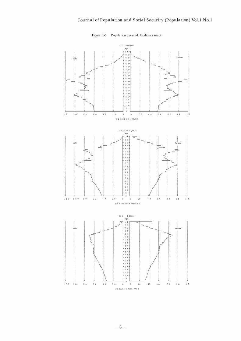
5. Changes in the Population Pyramid

The population pyramid for Japan continues to reflect the overall aging of the society, although it contains a jagged portion in the upper age groups that reflects the rapid variations in the fertility rate in the past (see Figure II-5). These include the sharp increase in the number of births between 1947 and 1949 (first baby boom) and the sudden drop in births between 1950 and 1957 (the "baby bust").

The population pyramid in 2000 has the first baby boom generation reaching their early 50s, and the second baby boom generation in their late 20s. By 2025 the first baby boomers will be in their late 70s, and the second baby boom generation will be reaching their early 50s. This makes it clear that the population aging up to 2025 will be primarily from the aging of the first baby boom generation. In comparison, the higher levels of elderly population in 2050 will be caused by a combination of the aging of the second baby boom generation and the contraction of the population in each generation due to the effects of the depressed fertility rate.

Hence, the population pyramid in Japan has shifted from its pre-war Mt. Fuji shape to its current temple bell shape and will continue to grow more top-heavy, becoming an urn shape in the future.

－5－

Journal of Population and Social Security (Population) Vol.1 No.1

0 020 2040 4060 6080 80100 100120 120

0

5

10

15

20

25

30

35

40

45

50

55

60

65

70

75

80

85

90

95

100

歳

男 女

(1) 2000 year

population (10,000)

age

FemaleMale

Figure II-5　　Population pyramid: Medium variant

0 020 2040 4060 6080 80100 100120 120

0

5

10

15

20

25

30

35

40

45

50

55

60

65

70

75

80

85

90

95

100

歳

男 女

(2) 2025 year

population (10,000)

Femele

age

Male

0 020 2040 4060 6080 80100 100120 120

0

5

10

15

20

25

30

35

40

45

50

55

60

65

70

75

80

85

90

95

100

歳

男 女

(3) 2050 year

population (10,000)

Female

age

Male

－6－

Journal of Population and Social Security (Population) Vol.1 No.1 6. Population Dependency Ratio Trends

The population dependency ratio is used as an index to express the level of support from the working-age group, through comparison of the relative size of the child and elderly populations versus the working-age population. According to the medium variant projection, the elderly population dependency ratio (calculated by dividing the elderly population by the working-age population) is

expected to rise from the current level of 26% (3.9 working-age people for each elderly person) to the 50% range in 2030 (2 workers for each senior citizen), continuing up to 67% (1.5 to 1) in 2050 (see Figure II-6). On the other hand, the child population dependency ratio (calculated by dividing the child population by the working-age population) is expected to shift from the current 21% (4.7 working-age people for each child) to a level between 19% and 21% in the future.

Although the low variant scenario leads to a decrease in the population of children due to the low fertility rate, no large drop is expected in the child dependency ratio. This is because the working-age population

that includes the parents of these children also declines.

0

10

20

30

40

50

60

70

80

90

1950 1960 1970 1980 1990 2000 2010 2020 2030 2040 2050

Year

(%)

Actual Projected

Overalldependency ratio

Old-age dependencyratio

Child depecdency ratio

Figure II-6　　Trends in age dependency: Medium Variant

The sum of the child dependency ratio and the elderly dependency ratio is called the population dependency ratio, which is an indicator of the total degree of burden on the working-age population. The overall population dependency ratio increases along with the increase in the elderly dependency ratio. As the working-age population contracts, the population dependency ratio is expected to rise from the current 47% to 67% in 2022, and to 87% in 2050. 7. Trends in Birth and Death Numbers and Rates

For the medium variant scenario, the crude death rate (mortality per thousand of population)

continues to rise from 7.7‰ (per mil) in 2001, to 12.1‰ in 2020, reaching 16.2‰ in 2050 (see Figure II-7). The reason for the continuing increase in crude death rate in spite of the continuing increases in the life expectancy is the expected rapid aging of Japan's population means a rapid increase in the proportion of the elderly population, which has a high rate of mortality.

－7－

Journal of Population and Social Security (Population) Vol.1 No.1

The crude fertility rate (births per thousand) is expected to decline from 9.4‰ in 2001 to 8.0‰ in 2013. The crude fertility rate will continue to decline in subsequent years to 7.0‰ in 2035 and 6.7‰ in 2050.

-10

-5

0

5

10

15

20

25

30

1950 1960 1970 1980 1990 2000 2010 2020 2030 2040 2050Year

Crude death rate

　Crude birth rate

Crude rate of natural increase

(‰)

Actual Projected

Figure II-7　　Crude birth rate, crude death rate, and crude rate ofnatural increase: Medium Variant

The crude rate of natural increase, which is the difference between the crude fertility rate and the crude death rate, is expected to remain positive for a while and was at 1.7% in 2001. In 2006, however, it is expected to become negative, eventually dropping to –9.5% in 2050.

According to this medium variant projection, it is expected that the number of annual births continue to decrease from the 1.19 million in 2001, falling below 1.1 million in 2008 and dropping below the million mark in 2014 to 670,000 in 2050 (see Figure II-8).

-1,000

-500

0

500

1,000

1,500

2,000

2,500

1950 1960 1970 1980 1990 2000 2010 2020 2030 2040 2050Year

Deaths

Live births

(1,000)

Natural increase

Actual Projected

Figure II-8　　Live births, deaths, and natural increase:Medium Variant

It is, on the other hand, expected that the number of deaths steadily increase from 980,000 in 2001 to 1.51 million in 2021, with peaking at 1.7 million in 2038. The subsequent annual numbers of deaths are expected to decrease slightly, reaching 1.62 million in 2050.

－8－

Journal of Population and Social Security (Population) Vol.1 No.1 III. Projection Methodology and Assumptions

The future population size and age-sex distribution can be determined if the future number of deaths by age and sex, future births including sex ratio, and international migrations are all known. Therefore, the future population of Japan is projected by assuming values for the future mortality, fertility with sex ratio at birth, and international migration. The projection methodology and assumptions are described below. 1. Projection Method

The usual cohort component method has been used as the projection method. This method uses the population by age and sex in the base year as the starting point, to which the assumed survival rates by age and sex, international migration (rate) by age and sex, female fertility rates by age, and ratio of sexes at birth are applied to determine a future population. Figure III-1-1 shows the basic calculation procedure for the cohort component method.

Let's consider the case of the

calculation for the population in the next year (t + 1) based on the known population by age and sex in year t. First, the population aged one-year or more in year t + 1 can be found by applying the corresponding survival and international migration rates to each age and sex classification in the population in year t. The number of new births of each sex is obtained by multiplying the number of women by their age-specific fertility rates, and applying the sex ratio at birth. The survival and international migration rates are then applied to determine the population by sex under age one in year t+1. The sum of these values is the projected population in year t+1.

Basically, the population that has reached each age of x years in the base year is multiplied by the assumed survival rate until age x + 1. This is then adjusted by the number (rate) of international migration of people for that age group. In this way the population as of October 1 the following year at age x + 1 is determined (by sex and age for each whole year between 1 and 99, as well as for the "100 and over" group). For the population of those under 1 year of age, first the average population of reproductive-age women (15 - 49) in the

Population by age/sex in year ｔ： N(x,t)

Population by age/sex in year t+1：

The numbers ofbirths by sex:B(x,t )

Ages 1 to 100+Age ０

Sex ratio at birth:SRB(t )

Age/sex-specificinternational migration

numbers (rates):NM(x,t )

Age/sex-specificsurvival rates：

S(x,t )=Lx +1/Lx

Female age-specificfertility rates:f (x,t )

t

t +1

Year

Figure III-1-1 Procedures for projecting population

－9－

Journal of Population and Social Security (Population) Vol.1 No.1 base year and subsequent year is determined. The average population in each age group is multiplied by the age-specific fertility rate to obtain the number of births for that year. The numbers of male and female births are determined using the sex ratio at birth. Finally, by multiplying by the corresponding survival rates, and making the adjustments for international migration the population under age 1 year as of October 1 the following year is determined.

The future annual population projections by age and sex are made by repeating this procedure. Therefore, the data required for the cohort component method used for this projection are (1) base population by age and sex, (2) assumed age-specific fertility rates, (3) assumed age- and sex-specific survival rates, (4) assumed age- and sex-specific international migration numbers (rates), and (5) assumed sex ratio at birth. 2. Base Population

The base population that forms the starting point for the projection is the total population as of October 1, 2000 (including non-Japanese residents) classified by age and sex. This population is based on the age and sex-specific population data obtained from the 2000 National Census, with adjustments to include the "age unknown" population on the census. Therefore, there are slight differences between the numbers for the base population in each age group used for this projection and the official statistics reported by the National Census. This point should be kept in mind when making use of the projection values. 3. Fertility Rate Assumptions

When projecting a future population by means of the cohort component method, the number of live births for each future year is essential. Only the number of live births in each year is taken as the total number of infants borne by women of reproductive age (from 15 - 49 years) in that year. The number of births by females in each age group is calculated by multiplying the female population in each age group by the corresponding age-specific fertility rate. This section will explain the method for estimating the age-specific fertility rates for females.3 However, fertility rate estimations are based on several assumptions about future trends in marriage and childbearing. For these assumptions to be accurate, we must understand the fertility trends in recent years in Japan. Therefore, let us begin with an overview of the recent fertility trends, and then consider the future prospects. (1) Recent fertility trends

The Total Fertility Rate (TFR)4 in Japan has declined each year since 1973, with a temporary increase between 1982 and 1984. In 1989 the TFR was 1.57, even lower than in 1966, which was an

3 The fertility rates used for the population projections are indices for the entire population, including non-Japanese residents (total population fertility rate). However, when setting the assumptions, since the official numbers from the past are only for Japanese citizens, it is made for Japanese fertility rates. The total population fertility rate calculation is discussed in section 5. 4 Sum of female age-specific fertility rates observed in a certain calendar year. These fertility rates are equivalent to the average number of live births that are expected if the females remain fertile according to the given age-specific fertility rates of the year.

－10－

Journal of Population and Social Security (Population) Vol.1 No.1

inauspicious "Hinoeuma" year, and had previously had the lowest TFR since Japan began recording vital statistics. Since then, TFR has continued to sink, with some fluctuations, reaching 1.36 in 2000 (see Figure III-3-1).

In Japan there has been a sharp decline in the rate of marriage among the age groups in the main childbearing years. Since extra-marital childbearing is infrequent here 5 , this drop in marriage rate can be considered the direct cause of the decline in fertility rates. Consider the group that has a large influence on TFR changes, women

in their late 20s. In 1970, 80.3% of women in this group were married, but by 2000 this had dropped to 43.5%. The proportion of the widowed and the divorced can contribute to changes in the proportion married in general; in fact, the proportion of never married women soared from 18.1% in 1970 to 54.0% in 2000, while the percentage of the divorced or the widowed changed only from 1.5% to 2.5% over the same period, so it can be claimed that the sharp increase in the proportion never married is the cause of the drop in the proportion married (Refer to Figure III-3-2 regarding trends in the proportion never married). A primary factor in the increase in the proportion never married since the late 1970s is the large increase in the never-married population in their 20's, indicating a tendency to delay marriage, in other words, an increase in the mean age at first marriage. In the 1980s, however, since the proportion never married continued to show increases even among those in their 30's and older, it became more likely that there is a continuing trend of never marrying throughout life, that is, an inThis agrees with the observed trends in marriage in rand never marrying tendencies.

0.0

0.5

1.0

1.5

2.0

2.5

3.0

3.5

4.0

1950 1955 1960 1965 1970 1975 1980 1985 1990 1995 2000Year

Tota

l fer

tility

rate

Figure III-3-1　The total fertility rate, 1950-2000

Source: Vital Statistics of Japan

Figure III-3-2　　Population never married of women by

Let us now consider the decrease in the number with the drop in the proportion married due to thdecrease in the fertility rate. Figure III-3-3 sho

－11－

5 In 2000 only 1.6% of all births were extra-marital.

crease in the proportion never married at age 50. ecent years, i.e., the increase of delayed marriage

0

10

20

30

40

50

60

70

80

90

100

1950 1955 1960 1965 1970 1975 1980 1985 1990 1995 2000

Year

Prop

ortio

n ne

ver m

arrie

d （％

）

age 15-19

age 20-24

age 25-29

age 30-34

age 35-39

age 40-44

age 45-49

age group, 1950-2000

Souece : Census of Japan

of children produced by a married couple along ese marriage behavior trends as a cause of the ws the annual changes in the number of first

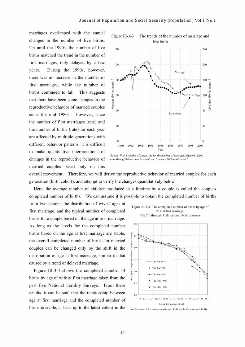
Journal of Population and Social Security (Population) Vol.1 No.1 marriages overlapped with the annual changes in the number of live births. Up until the 1990s, the number of live births matched the trend in the number of first marriages, only delayed by a few years. During the 1990s, however, there was an increase in the number of first marriages, while the number of births continued to fall. This suggests that there have been some changes in the reproductive behavior of married couples since the mid 1980s. However, since the number of first marriages (rate) and the number of births (rate) for each year are affected by multiple generations with different behavior patterns, it is difficult to make quantitative interpretations of changes in the reproductive behavior of married couples based only on this overall movement. Therefore, we will derive the reproductive behavior of married couples for each generation (birth cohort), and attempt to verify the changes quantitatively below.

Source: Vital Statistics of Japan. As for the number of marriage, adjusted valuesconsidering "delayed notifications" and "January 2000 notification."

Figure III-3-3　　The trends of the number of marriage andlive birth

0

20

40

60

80

100

120

1960 1965 1970 1975 1980 1985 1990 1995 2000Year

Mar

riage

（10

thou

sand

s）

0

40

80

120

160

200

240

Live

birt

h（10

thou

sand

s）

Marriage

Live births

Here, the average number of children produced in a lifetime by a couple is called the couple's completed number of births. We can assume it is possible to obtain the completed number of births from two factors; the distribution of wives’ ages at first marriage, and the typical number of completed births for a couple based on the age at first marriage. As long as the levels for the completed number births based on the age at first marriage are stable, the overall completed number of births for married couples can be changed only by the shift in the distribution of age at first marriage, similar to that caused by a trend of delayed marriage.

0.0

0.5

1.0

1.5

2.0

2.5

3.0

～19 20～21 22～23 24～25 26～27 28～29 30～31 32～33 34～35 36～

Age at first marriage of wife

The

coup

le's

com

plet

ed n

umbe

r of b

irths

on

aver

age

The 7th(1977)

The 8th(1982)

The 9th(1987)

The 10th(1992)

The 11th(1997)

Figure III-3-4　The completed number of births by age ofwife at first marriage:

The 7th through 11th national fertility survey

Note: For wives of first marriage couples aged 40-49 (for the 7th, wives aged 40-44).

Figure III-3-4 shows the completed number of births by age of wife at first marriage taken from the past five National Fertility Surveys. From these results, it can be said that the relationship between age at first marriage and the completed number of births is stable, at least up to the latest cohort in the

－12－

Journal of Population and Social Security (Population) Vol.1 No.1 graph (age 40 in 1997, namely the cohort born in the mid 1950's). If we can assume that this stable relationship is maintained in subsequent cohorts, then the completed number of births for the younger generations should vary only according to changes in the distribution of the age at first marriage, as has been the case in the past.

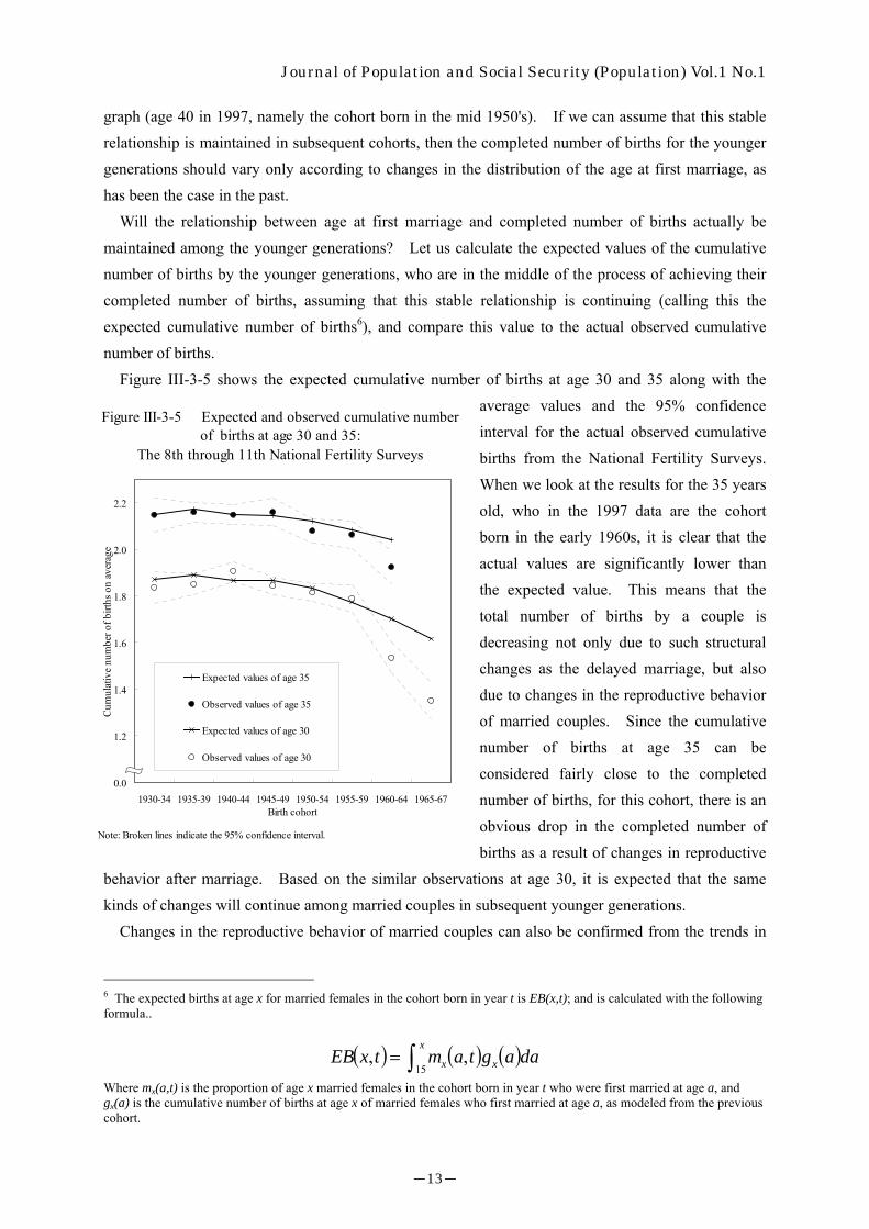
Will the relationship between age at first marriage and completed number of births actually be maintained among the younger generations? Let us calculate the expected values of the cumulative number of births by the younger generations, who are in the middle of the process of achieving their completed number of births, assuming that this stable relationship is continuing (calling this the expected cumulative number of births6), and compare this value to the actual observed cumulative number of births.

Figure III-3-5 shows the expected cumulative number of births at age 30 and 35 along with the average values and the 95% confidence interval for the actual observed cumulative births from the National Fertility Surveys. When we look at the results for the 35 years old, who in the 1997 data are the cohort born in the early 1960s, it is clear that the actual values are significantly lower than the expected value. This means that the total number of births by a couple is decreasing not only due to such structural changes as the delayed marriage, but also due to changes in the reproductive behavior of married couples. Since the cumulative number of births at age 35 can be considered fairly close to the completed number of births, for this cohort, there is an obvious drop in the completed number of births as a result of changes in reproductive

behavior after marriage. Based on the similar observations at age 30, it is expected that the same kinds of changes will continue among married couples in subsequent younger generations.

0.0

1.2

1.4

1.6

1.8

2.0

2.2

1930-34 1935-39 1940-44 1945-49 1950-54 1955-59 1960-64 1965-67Birth cohort

Cum

ulat

ive

num

ber o

f birt

hs o

n av

erag

e

Expected values of age 35

Observed values of age 35

Expected values of age 30

Observed values of age 30

Figure III-3-5　　Expected and observed cumulative numberof births at age 30 and 35:

The 8th through 11th National Fertility Surveys

Note: Broken lines indicate the 95% confidence interval.

Changes in the reproductive behavior of married couples can also be confirmed from the trends in

6 The expected births at age x for married females in the cohort born in year t is EB(x,t); and is calculated with the following formula..

( ) ( ) ( )daagtamtxEB x

x

x ,,15∫=

Where mx(a,t) is the proportion of age x married females in the cohort born in year t who were first married at age a, and gx(a) is the cumulative number of births at age x of married females who first married at age a, as modeled from the previous cohort.

－13－

Journal of Population and Social Security (Population) Vol.1 No.1 cumulative births in each year of marriage. Table III-3-1 shows the cumulative number of births in the seventh year of marriage as well as the distribution of births. In order to exclude the effects of delayed marriage, the sample for this table was limited to couples in which the wife's age at first marriage was between 23 and 27 years. For the 1940's cohorts, the percentage of couples without any children after 7 years is roughly 4%, rising to 8.4% for the cohort born in 1960~1964. As a result, the cumulative number of births also dropped from 1.96 to 1.80.

None 1 2 3 4 or over

1935-39 950 24.5 1.86 3.9 20.2 63.2 11.7 1.11940-44 2,031 24.5 1.96 3.8 13.9 64.8 16.9 0.51945-49 3,346 24.4 1.93 4.4 14.8 65.0 15.2 0.61950-54 2,910 24.5 1.95 4.5 14.5 63.1 17.2 0.71955-59 1,755 24.5 1.88 7.4 14.5 61.1 16.6 0.41960-64 833 24.5 1.80 8.4 19.3 57.0 14.8 0.5

NWive's cohortDistribution(%)Cumulative number of

births in the seventhyear of marriage

Mean age offirst marriage

Table III-3-1 Cumulative number of births in the seventh year of marriage:The 8th through 11th National Fertility Surveys

Note : For the first marriage couples in which the wife's age at marriage was between 23 and 27 years and the maritalduration was 7 years or over.

Based on the investigation above, estimates of the future fertility rates cannot only assume delayed marriage and a trend to not marry, but must also take into account that there will be changes in the reproductive behavior of couples after marriage. The method for determining these future developments is discussed in III-3-(3). Before that, let us first consider how to obtain the future age-specific fertility rates if such assumptions are made. (2) Age-specific fertility rate estimation method

Future age-specific fertility rates in each calendar year can be found by rearranging fertility rates for the corresponding female cohorts. Since the age-specific fertility rate at age x for a female in any given year is the age-specific fertility rate at age x for the female cohort born x years ago, the age-specific fertility rates covering all females of reproductive age (15 ~ 49) in that year can be obtained as a set of fertility rates for each age of the 35 cohorts born between 15 and 49 years ago. For this projection the age-specific fertility rates are estimated for each cohort, and then recombined to make the

－14

0.00

0.05

0.10

0.15

0.20

15 20 25 30 35 40 45 50

Age

Ferti

lity

rate

Actual

Predicted

Total

1st child

2nd child

3rd child

4th child or later

Figure III-3-6 　Cohort age-specific fertility rates(actual and predicted values): Women born in 1955

－

Journal of Population and Social Security (Population) Vol.1 No.1 age-specific fertility rates for each year (cohort fertility rate method). The reason for first estimating the cohort fertility rate is that the age patterns of fertility are generally more stable for the cohorts.

The age-specific fertility rates for a cohort are estimated using a suitable mathematical model with several parameters to represent the features of marriage and reproductive behaviors. Specifically, the fertility rates are estimated using a generalized log-gamma distribution model, with parameters such as the proportion never married at age 50 for the cohort, completed number of births, mean age at first marriage, and the mean age at birth for each birth order7. In this way we obtain a projection system that allows a representation of the basic patterns of change in the cohort fertility rate, including the most recent characteristics of reproductive behavior in Japan like delayed marriage, delayed childbearing, the anticipated future increase in the proportion of women who are never married at age 50, and the drop in the female completed number of births that reflects the drop in the number of children that couples have.

Figure III-3-6～8 presents a comparison between the age-specific fertility rates for three

7 In this model, the fertility rate (fn) for each birth order (n) is f

following expression is formed:

( ) (nnn xCxf γ⋅=

Where

( ) ( )

Γ=

−

nnn

nnnnn exp

b,b,u;x

n

λλλλ

λγ

λ

22

11

2

Γ and exp are a gamma function and an exponential function,each birth order (n). This formula is an extended version of thone type of generalized logarithm gamma distribution formula.The birth order consists of four groups, the 1st through the 3rd itself places limits on the reproducibility of actual age-specific actual results of fertility rates in Japan, we have made some mo

As a result, the （ ）fertility rate function by age of cohf x( )

( ) (∑=

⋅=

4

1nnnn b,u;xCxf γ

For more details, see the following reference: Ryuichi Kaneko, Rates(in Japanese with English summary)", Jinko Mondai KenkApril 1993, pp.17-38.

－15－

0.00

0.05

0.10

0.15

0.20

15 20 25 30 35 40 45 50Age

Ferti

lity

rate

Total

1st child

2nd child

3rd child

4th child or later

Actual

Predicted

Figure III-3-7 　Cohort age-specific fertility rates(actual and predicted values): Women born in 1965

irst given as a function of age (x). That is to say, the

)nnn ,b,u; λ

−−

−

n

nn

nn

n

n buxexp

bux

λλ2

11

respectively. ， ， , and Cn un bn λn are parameters of e expression known as the Coale-McNeill Model, which is

child, and the 4th child or later. However, the method fertility rates by age. Therefore, using error analysis with difications by extracting a standard error pattern（εn x( )）. ort can be calculated from the following expression:

)

−+

n

nnnn b

ux, ελ

" A Projection System for Future Age-Specific Fertility yu（Journal of Population Problems）, No.1, Volume 49,

Journal of Population and Social Security (Population) Vol.1 No.1 cohorts simulated with this model and the actual values.8

The fertility rates are simulated according to birth orders (from 1st child to 4th child or later), and the sum is used to obtain the age-specific fertility rates. By using actual values available as of 2000, actual fertility rates for women up to age 45, age 35, and age 25, respectively, can be obtained for (a) the cohort born in 1955, (b) the cohort born in 1965, and (c) the cohort born in 1975.

For group (a), it is likely that fertility will have almost been completed, so the period remaining for the projection is rather short. Group (b), on the other hand, is now in the midst of their reproductive phase. Since the overall fitness of the model is considered to be quite good, and considering the general stability of age patterns of fertility, it is likely that future fertility rates (for subjects 36 years old or older) will not divert much from the predicted values of the model.

For the (c) cohort, it is impossible to determine whether the model across the entire age range is good or bad from the fitness between the model and actual results so far. In fact, in cases (a) and (b), it is possible to identify model values (parameter values) using a formal statistics technique (maximum likelihood estimation method), and obtain relatively stable results. Applying the same method to the (c) group yields unstable results, and it is difficult to even specify a unique result. Obviously, this tendency is even more noticeable for younger cohorts who have experienced a shorter period of fertility. In order to estimate future fertility rates for these young cohorts, it is necessary to apply some external assumptions in order to compensate for the instability. In addition, for cohorts whose members are not even yet 15 years of age, it is impossible to determine future fertility rates using statistical methods because there are no actual fertility rate values. Consequently, for these younger (and still unborn) cohorts, assumptions have been made about the overall future fertility process. The method of specifying these assumptions is discussed in section III-3-(3).

0.00

0.05

0.10

0.15

0.20

15 20 25 30 35 40 45 50

Age

Ferti

lity

rate

Total

1st child

2nd child

3rd child

4th child or later

Actual

Predicted

Figure III-3-8 　Cohort age-specific fertility rates(actual and predicted values): Women born in 1975

If age-specific fertility rates for a series of cohorts are estimated by the aforementioned methods, age-specific fertility rates for each calendar year can be obtained by rearranging them according to age. For example, the fertility rate for ages 15 to 49 in year 2000 can be obtained by combining the fertility rate for the cohort of 15-year olds born in 1985, the fertility rate for the cohort of 16-year olds born in

8 The actual values of fertility rates used in the model estimation differ slightly from those released in the official vital statistics. For this model the total number of births between January and December was divided by the population on July 1, while the official statistics used the population on October 1 as the denominator. As a result of the annual adjustment of the age-specific fertility rate, coincidental variation and the inconsistencies in the denominators for the cohorts born in the Hinoeuma year (1996) were adjusted. Between 1966 and 1999 the populations used for the denominators were determined using backward projections based on the 2000 National Census data.

－16－

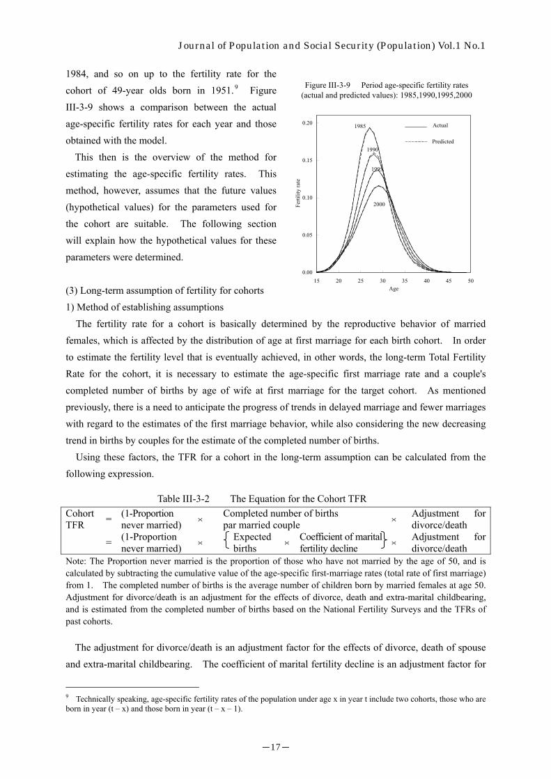
Journal of Population and Social Security (Population) Vol.1 No.1 1984, and so on up to the fertility rate for the cohort of 49-year olds born in 1951.9 Figure III-3-9 shows a comparison between the actual age-specific fertility rates for each year and those obtained with the model.

This then is the overview of the method for estimating the age-specific fertility rates. This method, however, assumes that the future values (hypothetical values) for the parameters used for the cohort are suitable. The following section will explain how the hypothetical values for these parameters were determined. (3) Long-term assumption of fertility for cohorts 1) Method of establishing assumptions

The fertility rate for a cohort is basically determined by the reproductive behavior of married females, which is affected by the distribution of age at first marriage for each birth cohort. In order to estimate the fertility level that is eventually achieved, in other words, the long-term Total Fertility Rate for the cohort, it is necessary to estimate the age-specific first marriage rate and a couple's completed number of births by age of wife at first marriage for the target cohort. As mentioned previously, there is a need to anticipate the progress of trends in delayed marriage and fewer marriages with regard to the estimates of the first marriage behavior, while also considering the new decreasing trend in births by couples for the estimate of the completed number of births.

Using these factors, the TFR for a cohort in the long-term assumption can be calculated from the following expression.

Table III-3-2 The Equation for the Cohort TFR

Cohort TFR = (1-Proportion

never married) × Completed number of births par married couple × Adjustment for

divorce/death

= (1-Proportion never married) × Expected

births ×Coefficient of marital fertility decline × Adjustment for

divorce/death

0.00

0.05

0.10

0.15

0.20

15 20 25 30 35 40 45 50Age

Ferti

lity

rate

1985

1990

1995

2000

Actual

Predicted

Figure III-3-9　　Period age-specific fertility rates(actual and predicted values): 1985,1990,1995,2000

Note: The Proportion never married is the proportion of those who have not married by the age of 50, and is calculated by subtracting the cumulative value of the age-specific first-marriage rates (total rate of first marriage) from 1. The completed number of births is the average number of children born by married females at age 50. Adjustment for divorce/death is an adjustment for the effects of divorce, death and extra-marital childbearing, and is estimated from the completed number of births based on the National Fertility Surveys and the TFRs of past cohorts.

The adjustment for divorce/death is an adjustment factor for the effects of divorce, death of spouse and extra-marital childbearing. The coefficient of marital fertility decline is an adjustment factor for

9 Technically speaking, age-specific fertility rates of the population under age x in year t include two cohorts, those who are born in year (t – x) and those born in year (t – x – 1).

－17－

Journal of Population and Social Security (Population) Vol.1 No.1 the decrease in the completed number of births that is accompanying the previously discussed changes in reproductive behavior of married couples. This yields the following expression.

( ) ( )( ) ( ) ( )( )( ) ( ) ( )( ) ( )twtktCEBtPS

twtCEBtPStCTFR

⋅⋅⋅−=

⋅⋅−=

α

β

50

50

1

1

For the cohort born in year t, CTFR(t) is the Cohort Total Fertility Rate, PS50(t) is the proportion never

married, CEBβ(t) is the completed number of births, and w(t) is the coefficient of divorce/death. CEBα(t) is the expected births based on the distribution of age at first marriage and the couple's completed number of births by age of wife at first marriage for the cohort, which is compensated using k(t) ,the coefficient of marital fertility decline. 2) Target cohort

The cohort of females used for setting the estimates is comprised of those who were 15 years of age as of 2000, that is, born in 1985. The reason this cohort was selected as the target cohort is that the marriage and reproductive behavior of this cohort will be completed at age 50, which will be 2035, allowing for estimations of fertility rates over a long term. At the same time, the cohort of 15-year-old females should exhibit behaviors that do not deviate too greatly from the extensions of recent changes in marriage and reproductive behaviors. However, the changes in marriage and reproductive behaviors that become noticeable among women in their 30s are also underway among those in their 20's, so there is a high probability that this kind of change will continue in the cohorts born after 1985. Accordingly, we assumed that the forces of change did not completely halt in 1985 when the target cohort was born, and cohort fertility rates have been projected to converge on the cohort born in 2000. This year 2000 cohort is called the ultimate cohort. The cohorts born in 2001 and later are generations that were not born as of 2000. It would be difficult to predict the changes in marriage and birth behavior for these females based on the current changes in marriage behavior. Therefore, for these projections, for cohorts born in 2001 and later, the fertility rates will be fixed to the 2000 levels. 3) Estimating the proportion never married and the mean age at first marriage for the target cohort.

Before estimating the first marriage rates of the target cohort (cohort born in 1985), the age-specific first marriage rates for each birth cohort of females born in and after 1935 were calculated.10

Next, based on the first marriage rates for these cohorts, the mean age at first marriage and the proportion never married was estimated for each cohort. When making the projections, it is naturally possible that there will be a first marriage at a later age for members of cohorts that have not yet

10 Since there is a delay in official registration of marriages in the number of first marriages obtained from vital statistics, we account for this delay in registration when calculating the age-specific first-marriage rates. The concentration of official registrations in January 2000 is considered a transient effect, and the first-marriage rate for 1999 and 2000 was modified by adjustment of the number of first marriages in December 1999 and January 2000.

－18－

Journal of Population and Social Security (Population) Vol.1 No.1

completed their marriage behavior, for example the cohort born in 1965, at age 35 in 2000. For these birth cohorts the first-marriage rate distribution for those age 35 years or older was estimated using a generalized log-gamma distribution model. The relationship between the mean age at first marriage and the proportion never married, for each cohort born from 1935 to 1965, is shown in Figure III-3-10

The points indicated by × in the figure are the mean age at first marriage and proportion never married for those born between 1935 and 1951. These show a stable pattern of nearly universal marriage at a young age, with a mean age at first

marriage of about 24 and proportion never married of about 5%. The ● marks indicate the points for the cohorts born between 1952 and 1964. These cohorts show a gradual rise in both the mean age at first marriage and the proportion never married. The values for the cohorts born between 1965 and

1970, indicated by the ◯ marks, show the same increasing tendency, but there is a change in the relationship between the two, with the proportion never married increasing at a more rapid rate. The future results for mean age at first marriage and the proportion never married for the cohort born in 1985 are expected to be along the extension of the line of the trends of changes displayed by the cohorts born between 1965 and 1970.

4%

5%

6%

7%

8%

9%

10%

11%

12%

13%

14%

24.0 24.5 25.0 25.5 26.0 26.5 27.0 27.5 28.0

Mean Age at first marriage

Pro

port

ion n

ever

mar

ried

Cohorts born in 1935～51

Cohorts born in 1952～64

Cohorts born in 1965～70

Figure III-3-10　　Mean age at first marriage and proportionnever married for cohorts born in 1935 or later

Assuming that the age-specific fertility rates for the target cohort (born in 1985) are an extension of past changes, it is then necessary to concretely specify either the mean age at first marriage or the proportion of permanently single. Here, the proportion never married is obtained from projections based on national vital statistics. That is, the rate of change in the never-married rate for each 5 year age grouping both nationally and by prefecture over the past 5 years (1995 to 2000) is extended to project the future proportion never-married at age 50 (cohort rate of change method). The proportion of 0

10

20

30

40

50

60

70

80

90

100

15～19 20～24 25～29 30～34 35～39 40～44 45～49 50

age

Pro

port

ion n

ever

mar

ried

（％

）

1901～1905 1906～1910

1911～1915 1916～1920

1921～1925 1926～1930

1931～1935 1936～1940

1941～1945 1946～1950

1951～1955 1956～1960

1961～1965 1966～1970

1971～1975 1976～1980

1981～1985

Figure III-3-11　　Estimation of proportion never married offemale by age group and birth cohort

－19－

Journal of Population and Social Security (Population) Vol.1 No.1 permanently single is taken as the average of the rates for the 45 ~ 49 year old group and the 50 ~ 54 year old group (see Figure III-3-11).

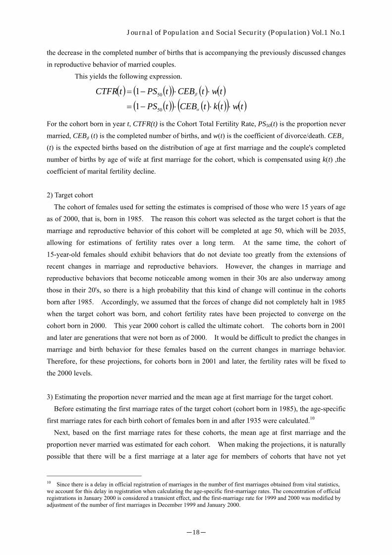
Since there are large uncertainties in the factors related to the trends for the mean age at first marriage and proportion of permanently single, three variants for the assumptions have been made, a medium, high, and low variant. First, the national value of 16.8% for the 1985 cohort11 is adopted as the proportion never married at age 50 for the medium variant. The mean age at first marriage is obtained as 27.8 from the relationship between the proportion never married at age 50 and the mean age at first marriage for cohorts born since 1965. For the low variant projection, it is assumed that there will be the greatest progress in delayed marriage and increases in the proportion never married. Among socioeconomic groups in modern Japan, the group with the highest mean age at first marriage is the female population of Tokyo. Assuming that the target cohort adopts the same marriage behavior as this group, this yields a proportion never married of 22.6%. For the mean age at first marriage, using the relationship between the proportion never married and the mean age at first marriage in the same way as for the medium variant, the value for the low variant is 28.7 years. For the high variant projection, the estimates are made based on the assumption that the changes in marriage behavior in the future will not progress to any great degree. For this case, the average of the 10 lowest values is used, yielding a proportion never married of 13.3%, leading to a mean age at first marriage of 27.3 years (Figure II-3-12). 4) Calculation of expected completed bi

Using the mean age at first marriageexpected completed births for married c

11 The proportion never married for the cohort bproportion never married at age 50 for the 1976~

PSPS ii 85198150

198550 ⋅≅ −

1) Yamagata, Fukushima, Ibaragi, Tochigi, Gunma, Fukui, Yamanashi, Gifu, Mie, Shiga

4%

6%

8%

10%

12%

14%

16%

18%

20%

22%

24%

24.0 24.5 25.0 25.5 26.0 26.5 27.0 27.5 28.0 28.5 29.0 29.5Mean age at first marriage

Prop

ortio

n ne

ver m

arrie

d at

age

50

28.7

Assumption for low variant:Proportion never married at age 50among females in Tokyo（22.6％）

27.8

Assumption for medium variant:National value for proportionnever married at age 50（16.8％）

27.3

Assumption for high variant:Proportion never married atage 50 among females in the10 lowest areas（13.3％）

Figure III-3-12　　Mean age at first marriage and proportionnever married for a cohort born in 1985

rths for the target cohort assumed for each of the medium, high and low variants, the ouples was calculated for the target cohort as described below.

orn in 1985 was estimated using the following expression with the 1980 cohort and the 1981~1985 cohort.

( )( ).rexp 519831985−⋅ ,

⋅=−

−

80197650

85198150

51

PSPSlnr i

i

－20－

Journal of Population and Social Security (Population) Vol.1 No.1 First, the average completed births according to age at first marriage obtained from the data from the National Fertility Surveys is used to generate a model by birth order, and a lifetime birth probability by age at first marriage and birth order is determined. Then, this probability and the previously projected distribution of ages at first marriage are used to determine the total completed number of births by married females in the target cohort.12 With this method the expected births for the

distribution of ages at first marriage for the target cohort, CEBα(1985), is found to be 1.89 for the medium variant, 1.93 for the high variant, and 1.81 for the low variant. 5) Setting the coefficient of effect of divorce/death and the coefficient of marital fertility for the target cohort

After setting the fertility rates for the

target cohort using the previously-discussed cohort total fertility rate formula, the remaining factors are the coefficient of effect of divorce/death and the coefficient of marital fertility. For the coefficient of effect of divorce/death, w(1985), since the past values obtained from the Basic Fertility Surveys and vital statistics are stable across cohorts, the average value of 0.971 is used.

The coefficient of marital fertility k(1985) is estimated as follows. First, a generalized log-gamma distribution model is used with various specified levels for k(1985) to estimate the age-specific cohort

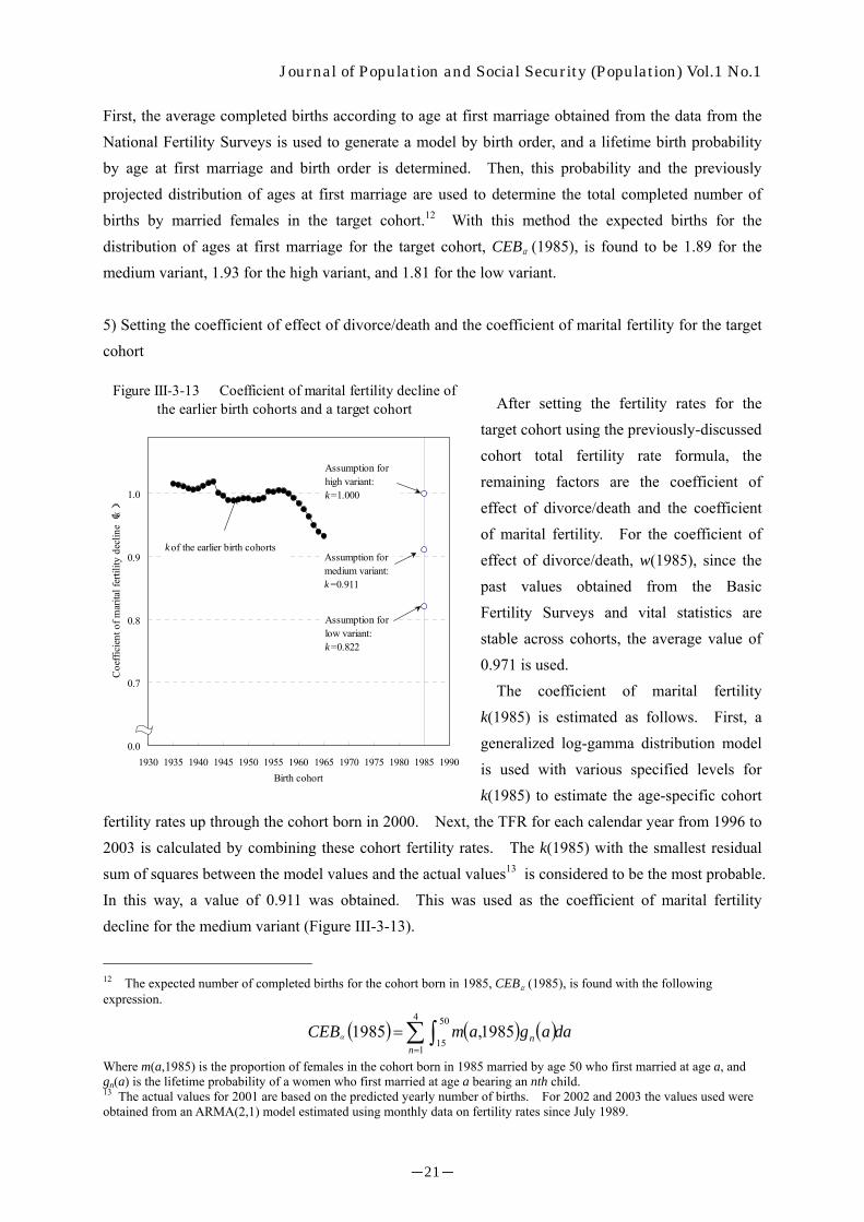
fertility rates up through the cohort born in 2000. Next, the TFR for each calendar year from 1996 to 2003 is calculated by combining these cohort fertility rates. The k(1985) with the smallest residual sum of squares between the model values and the actual values13 is considered to be the most probable. In this way, a value of 0.911 was obtained. This was used as the coefficient of marital fertility decline for the medium variant (Figure III-3-13).

0.0

0.7

0.8

0.9

1.0

1930 1935 1940 1945 1950 1955 1960 1965 1970 1975 1980 1985 1990Birth cohort

Coe

ffici

ent o

f mar

ital f

ertil

ity d

eclin

e（

k）

Assumption forhigh variant:k =1.000

Assumption formedium variant:k =0.911

Assumption forlow variant:k =0.822

k of the earlier birth cohorts

Figure III-3-13　　Coefficient of marital fertility decline ofthe earlier birth cohorts and a target cohort

12 The expected number of completed births for the cohort born in 1985, CEBα(1985), is found with the following expression.

( ) ( ) ( )∑∫=

=4

1

50

151985,1985

nn daagamCEBα

Where m(a,1985) is the proportion of females in the cohort born in 1985 married by age 50 who first married at age a, and gn(a) is the lifetime probability of a women who first married at age a bearing an nth child. 13 The actual values for 2001 are based on the predicted yearly number of births. For 2002 and 2003 the values used were obtained from an ARMA(2,1) model estimated using monthly data on fertility rates since July 1989.

－21－

Journal of Population and Social Security (Population) Vol.1 No.1

The coefficient of marital fertility decline for the high variant is obtained by assuming that k for the cohort born in 1985 will return to a level of 1.00. In comparison, for the low variant, in consideration of the rapid decline in marital fertility since the 1965 cohort, it is assumed that k will be equal to the level for the medium variant minus the difference between the high variant and the medium variant, that is reaching a level of 0.822. Since the estimated completed number of births obtained from the distribution of age at first marriage is 1.89 for the medium variant, 1.93 for the high variant, and 1.81 for the low variant (III-3-(3)-4)), each of these values is multiplied by the corresponding value of k to obtain the completed number of births by a married couple of 1.72 under the medium variant, 1.93 under the high variant, and 1.49 under the low variant. 6) Estimates of the target cohort fertility rates

From the proportion never married, mean age at first marriage, expected number of births by a couple, and adjustment for divorce/death estimated for the target cohort, using the previously derived expression to calculate the total fertility rate for the target cohort leads to a value of 1.39 for the medium variant, 1.62 for the high variant, and 1.12 for the low variant. Tables III-3-3 and III-3-4 summarize the assumed values for each of the factors for the target cohort and the total fertility rates.

Expectedbirths

Coefficient ofmarital fertility

decline

Medium 16.8 27.8 1.72 1.89 0.911 0.971 1.39

High 13.3 27.3 1.93 1.93 1.000 0.971 1.62

Low 22.6 28.7 1.49 1.81 0.822 0.971 1.12

Assumptions CohortTFR

Completednumber of births

par marriedcouple

Adjustment fordivorce/death

Proportionnever

married（％）

Mean age atfirst marriage

Table III-3-3 Assumed values for nuptiality and fertility as well as total fertilityrates for female cohort born in 1985

None 1 2 3 4 or more

Medium 1.39 31.2 18.5 33.9 12.9 3.5 High 1.62 21.1 20.1 38.6 15.5 4.7 Low 1.12 42.0 17.5 29.1 9.3 2.1

Distrubution of live births（％）CohortTFRAssumptions

Table III-3-4 Assumed total fertility rates and distribution of live births for female cohort born in 1985

After setting the cohort TFR for the target cohort, the target cohort TFR was decomposed into

cohort TFRs by birth order according to the distribution of live births estimated beforehand. Under

－22－

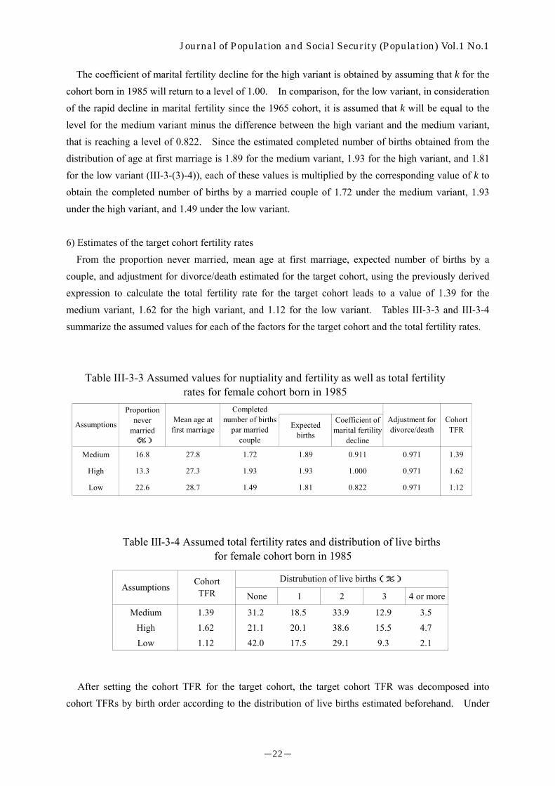
Journal of Population and Social Security (Population) Vol.1 No.1 the restrictions of being able to reproduce the mean and deviation of age at childbirth for the given year, the parameters for a generalized log-gamma model were determined so that there was no contradiction with the trends in parameters of first marriage rate and in that of preceding cohorts. If the parameters can be determined, the generalized log-gamma model can be used to predict the future values of the age-specific fertility rates by order of birth. Figure III-3-14 shows the cumulative fertility rates for each cohort predicted under the medium variant assumptions. The various indicators related to the cohort fertility rates and first marriagdistribution model are listed in Table III-3-5.

1950 1955 1960

5.0 5.0 7.4

24.4 24.9 25.6

1.98 1.97 1.84

10.0 12.3 16.4

12.4 11.7 13.6

52.1 47.4 44.1

21.0 23.4 21.1

4.5 5.1 4.8

27.6 28.1 28.7

1st 25.7 26.3 27.0

2nd 28.3 28.7 29.3

3rd 30.8 31.2 31.6

4th and more 33.1 33.6 34.1

Cohort indices

Mean age at first marriage

Cohort TFR

Proportion never married

None

1

2

Mea

n ag

e at

chi

ldbi

rth All

Dis

tribu

tion

4 or more

3

Note : Figures are based on the values predicted b

Table III-3-5 Vrious indicatorand first

(4) Assumed Annual Fertility Rate

If the age-specific cohort fertility rates are phigh, medium and low variants, it is possible to

e rates estimated using the generalized log-gamma

0.0

0.2

0.4

0.6

0.8

1.0

1.2

1.4

1.6

1.8

2.0

2.2

15 20 25 30 35 40 45 50Age

Cum

ulat

ive

age

spec

ific

ferti

lity

rate

19501955196019651970197519801985

Birthcohort

Note : Markers represent actual values.

Figure III-3-14　　Actual and predicted values forcumulative age specific fertility rates: Medium variant

1965 1970 1975 1980 1985 1990 1995 2000

9.2 12.5 15.8 16.6 16.8 16.9 17.0 17.0

26.6 27.1 27.6 27.8 27.8 27.9 27.9 27.9

1.65 1.50 1.42 1.40 1.39 1.39 1.39 1.39

21.9 27.7 29.9 31.0 31.2 31.2 31.3 31.3

15.6 15.8 18.1 18.4 18.5 18.6 18.6 18.7

41.9 38.9 35.3 34.2 33.9 33.8 33.7 33.7

16.4 13.8 13.0 12.9 12.9 12.9 12.9 12.9

4.2 3.8 3.6 3.5 3.5 3.5 3.5 3.5

29.5 30.1 30.7 30.9 31.0 31.0 31.0 31.1

27.8 28.4 29.0 29.2 29.2 29.3 29.3 29.3

30.3 31.1 31.7 32.0 32.1 32.2 32.3 32.3

32.3 33.1 33.7 33.9 33.9 33.9 33.9 33.9

34.7 35.1 35.3 35.4 35.4 35.4 35.4 35.4

Birth cohort

y the generalized log-gamma distribution model.

s related to the cohort fertility ratesmarriage rates

rojected based on the three sets of assumptions for the calculate the total fertility rate for a future period by

－23－

Journal of Population and Social Security (Population) Vol.1 No.1 making combinations of these cohort fertility rates. The year to year transitions are shown in Figure III-3-15. According to the projections based on the medium variant assumptions there will be a decrease from 1.36 in 2000 to 1.31 in 2007, followed by an increase to 1.39 in 2049. Under the high variant assumptions the TFR will immediately begin to rise from the 2000 level of 1.36, reaching 1.63 in 2049. The projections based on the low variant assumptions indicate that there will continue to be a drop from the 2000 level of 1.36 down to 1.10 in 2049.

0.0

0.5

1.0

1.5

2.0

2.5

3.0

3.5

4.0

1950 1960 1970 1980 1990 2000 2010 2020 2030 2040 2050Year

Tota

l fer

tility

rate

Actual Assumed

Medium variant

High variant

Low variant

Figure III-3-15　Actual and assumed total fertility rates,1950-2050

4. Survival Rate Assumptions (Future Life Table) (1) Methods of Estimating Survival Rates

In order to project a population for the following year using the cohort component method it is necessary to know the survival rates; meaning that future life tables must be generated from assumed future mortality rates. There are three main types of methods for assuming future mortality rates; the empirical method, the mathematical method, and the relational model method.

The empirical method makes use of the age-specific death rates that have been experienced in existing populations. An example of this is a "model life table" generated by classifying actual life tables with relatively high accuracy into similar groups, to estimate and also to project the life expectancy in developing countries where population statistics, including mortality data, are unreliable. The model life table method is still used to estimate the life tables in countries and regions that do not yet have adequately prepared population statistics.

In case of the population with the highest life expectancy at birth in the world, as is true in modern Japan, the problem with the empirical method is that populations as reference for the empirical values are limited. One way to get around this problem is the "best life table", which is a single life table composed by combining the lowest age-specific death rates achieved among several populations. Because these "best life tables" use age-specific death rates that are low but have already actually achieved in the real world, the future life tables are at levels that are likely to be achieved and are entirely realistic. To apply these best life tables to construct future life tables for Japan, it is necessary to come up with some innovation, e.g., combining the lowest age-specific death rates by the administrative areas of Japan, or combining the lowest age-specific death rates from the life tables of various countries throughout the world. For example, the "best life table" constructed using the life

－24－

Journal of Population and Social Security (Population) Vol.1 No.1 table classified by the administrative areas of Japan in 1995 shows the life expectancies of 79.27 years for males and 86.19 years for females. However, for any life table constructed by this method, the timing has to be specified when the life table that contains specific mortality rates will be achieved by the population of interest in the future.

For the mathematical method, the future mortality rates are estimated by fitting and extrapolating mathematical functions to the past mortality trends. Several variations exist according to what is used as the data for fitting functions. Simply fitting a mathematical function to the changes in life expectancy, however, does not allow us to generate the survival rates needed for population projection by the cohort component method. As explained below, other examples of estimating future mortality include extrapolation of age-specific mortality rates, extrapolation of age-specific mortality rates by cause of death, and extrapolation of standardized cause-specific mortality rates. The age-specific mortality rates were extrapolated in the 1981 round of population projections for Japan. The age-specific mortality rate extrapolation requires fitting multiple trend lines corresponding to the number of age categories. In contrast, extrapolating age-specific mortality rates by cause of death is more detailed than extrapolating the age-specific all-cause mortality rate. In this detailed way, trend lines are fitted to the age-specific mortality rates for each cause of death. This has the advantage of considering different tends in each cause of death. However, implementation is not straightforward. Even when the age and cause of death are broadly categorized, the extrapolation exercise can be very tedious. For example, two sexes, 18 age groups (5 year ranges), and 13 to 15 causes of death demand about 500 curve fittings. Thus, extrapolation of the standardized mortality rates by cause of death, a simplified version of extrapolation of the age-specific mortality rates by cause of death, was implemented for the population projections in 1986 and 1992. The procedure was to estimate future parameters of age-standardized mortality rates for each cause of death, then to uniformly apply these parameters to obtain age-specific mortality rates by cause of death. However, for the 1997 projection, the age was divided into four groups (0-14 years, 15-39 years, 40-64 years, 65 and over), and the projections were made with more detail reflecting the future parameter estimates standardized for the different age groups.

There are several concerns for projections by cause of death. Not only is fitting likely to be tedious, but there are also problems with the stability and regularity for the causes with a small number of deaths, making it difficult to fit a function. Moreover, problems arise in the continuity of cause of death trends due to revisions in the classifications of cause of death statistics14, requiring some adjustments. Since 1995, as a recent example, the 10th revision of International Statistical Classification of Diseases and Related Health Problems (ICD-10) has been implemented in Japan and modified the way that causes of death are classified. The Ministry of Health and Welfare (now Ministry of Health, Labour, and Welfare) created a conversion table between the reclassification of the 1994 mortality statistics into 130 items of ICD-10 and that into 117 items of ICD-9 (the 9th

14 It started in 1893 as the Bertillon Classification. For more details, see "Vital Statistics", Ministry of Health, Labour and Welfare.

－25－

Journal of Population and Social Security (Population) Vol.1 No.1 Revision).15 Evaluation is necessary, however, for the validity across all ages and whether it can be hold true to the past data. Besides the issues of gaps in the official classification, there can be changes in the cause of death recorded on death certificates as a result of changing ideas in society as certain causes of death were avoided or preferred for recording on death certificates due to social circumstances and/or stigma as well as the attitudes among the doctors.16 Also, the advancements and the innovations of medical technologies allow clearer identification of the cause of death, which in the past may have been attributed to somewhat ambiguous and less specific causes of death, such as senility or heart failure. Furthermore, projections based on the cause-specific mortality separately have possibilities of underestimation compared with projections based on all causes mortality.17

The relational model method can be considered a combination of the empirical method and the mathematical method, applicable to generating future life tables. A relational model describes the relationship between several empirical life tables using a small number of parameters. The future projections are made by mathematically extrapolating these parameters.

Brass developed a two-parameter model that described the relationship between multiple life tables,18 although the fit was not well for the very young and the older ages. Subsequently, there were attempts to improve the fit of model in the older age groups.19 The major disadvantage of the Brass model, with two parameters, was that it could not express different levels of mortality changes in different ages, which explains the abovementioned lower fits for the both extremes of age. On the other hand, other models with many parameters had to estimate correspondingly more parameters to cover the entire age range. Thus, it may bring along more sources of errors, even if the fitting is not tedious.

Lee and Carter have developed a model that restricts the number of parameters to one while improving the fit of the mortality changes across the age.20 By now a variety of applications have been studied. The Lee-Carter model is expressed as follows for age x at time t.++

txetkxbxatxm ,),ln( ++=

Here, ln(mx,t) is the log of the age-specific mortality rate, ax is the standard age-specific mortality schedule based on the average, kt is the mortality level index, bx expresses the age-specific change in

15 Statistics and Information Department, Ministry of Health and Welfare [Dai 10 Kai Shuseisiintoukeibunrui (ICD-10) to Dai 9 Kai Shuseisiintoukeibunrui (ICD-9) no Hikaku]. 16 For example, see Suyama Y. and H. Tsukamoto （1995） [Shi'in no Hensen ni Kansuru Shakaigakuteki Haikei] "Kousei no Shihyou" (Journal of Health and Welfare Statistics) Vol. 42 No. 7, pp 9-15. 17 Wilmoth, J.R. (1995), “Are mortality projections always more pessimistic when disaggregated by cause of death?” Mathematical Population Studies, 5, pp.293-319. 18 Brass, W. (1971), “On the scale of mortality,” Biological Aspects of Demography, ed., W. Brass, London: Taylor and Francis. 19 For example, Zaba, B. (1979), “The four-parameter logit life table system,” Population Studies, 33, pp. 79-100. Ewbank, D.C., J. C. Gomez De Leon, and M. A. Stoto (1983), “A reducible four-parameter system of model life tables,” Population Studies, 37, pp.105-127. Himes, C.L., S.H. Preston, and G.A. Condran (1994), “A relational model of mortality at older ages in low mortality countries,” Population Studies, 48, pp. 269-291 etc. 20 Lee, R.D. and L.R. Carter (1992), “Modeling and forecasting U.S. mortality,” Journal of the American Statistical Association, 87, pp.659-671.

－26－

Journal of Population and Social Security (Population) Vol.1 No.1 the mortality for change in kt 21, and ex,t indicates the residual. The advantage of this model is that it is possible to express a different rate of change for each age group simply by a single parameter kt. Lee and Carter calculated the parameters using mortality rates in the United States for age groups of 0 years, 1-4 years, 5-9 years, … , 80-84 years and 85 years and older. Then, using the time-series

analysis they determined the future values of the mortality index kt from 1990 through 2065. Although ARIMA (1,1,0) model was marginally superior, (0,1,0) model was adopted for the sake of

parsimony. After obtaining the future values for kt, the death rates were then computed. Since the oldest age group was 85 years and older, the final death rates for the 75-79 years and the 80-84 year age groups were used to determine the death rates up to age groups 105-109 years by the Coale and Guo method.22 (2) Future Life Table Estimation

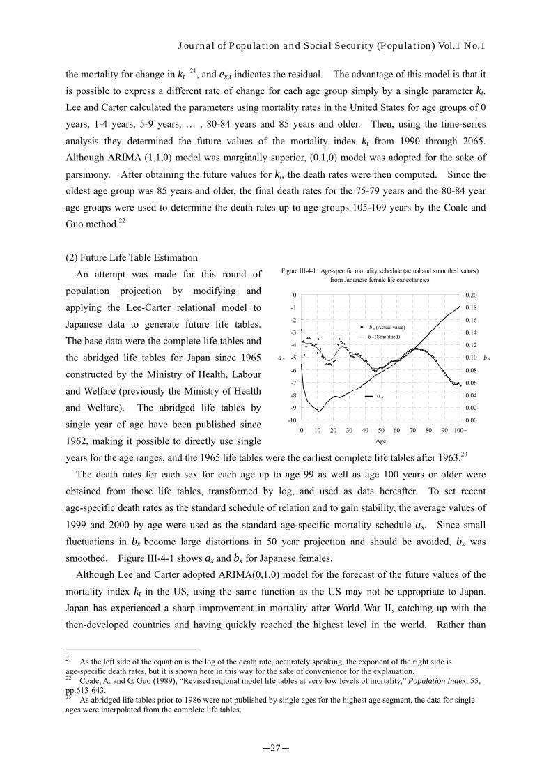
An attempt was made for this round of population projection by modifying and applying the Lee-Carter relational model to Japanese data to generate future life tables. The base data were the complete life tables and the abridged life tables for Japan since 1965 constructed by the Ministry of Health, Labour and Welfare (previously the Ministry of Health and Welfare). The abridged life tables by single year of age have been published since 1962, making it possible to directly use single years for the age ranges, and the 1965 life tables were the earliest complete life tables after 1963.23

Figure III-4-1　Age-specific mortality schedule (actual and smoothed values)from Japanese female life expectancies

-10

-9

-8

-7

-6

-5

-4

-3

-2

-1

0

0 10 20 30 40 50 60 70 80 90 100+Age

a x

0.00

0.02

0.04

0.06

0.08

0.10

0.12

0.14

0.16

0.18

0.20

b x

　a x

◆ b x (Actual value)

― b x (Smoothed)

The death rates for each sex for each age up to age 99 as well as age 100 years or older were obtained from those life tables, transformed by log, and used as data hereafter. To set recent age-specific death rates as the standard schedule of relation and to gain stability, the average values of

1999 and 2000 by age were used as the standard age-specific mortality schedule ax. Since small fluctuations in bx become large distortions in 50 year projection and should be avoided, bx was smoothed. Figure III-4-1 shows ax and bx for Japanese females.

Although Lee and Carter adopted ARIMA(0,1,0) model for the forecast of the future values of the

mortality index kt in the US, using the same function as the US may not be appropriate to Japan. Japan has experienced a sharp improvement in mortality after World War II, catching up with the then-developed countries and having quickly reached the highest level in the world. Rather than

21 As the left side of the equation is the log of the death rate, accurately speaking, the exponent of the right side is age-specific death rates, but it is shown here in this way for the sake of convenience for the explanation. 22 Coale, A. and G. Guo (1989), “Revised regional model life tables at very low levels of mortality,” Population Index, 55, pp.613-643. 23 As abridged life tables prior to 1986 were not published by single ages for the highest age segment, the data for single ages were interpolated from the complete life tables.

－27－

Journal of Population and Social Security (Population) Vol.1 No.1 assuming that Japanese mortality will continue to improve more rapidly than in the other developed countries, it would be more natural to assume that Japan’s trend will converge to gradual improvement as experienced elsewhere, as is the case in Sweden where low mortality has continued to improve with a modest change for the past 50 years.24 In fact, a close examination

of the change in the level of kt of Japanese data indicates that the rate of improvement over the last 30 years has been slowing down (Figure III-4-2). Accordingly, functions are fitted to reflect this trend in the future estimates. One of the functions considered was a logarithmic function whose change gradually becomes smaller but continues without an asymptote.25 Researchers who believe that life expectancy will continue to increase have been more vocal in the recent years, but a latest survey in Japan among population experts showed that Japanese experts tended to believe the increase in the life expectancy of Japanese would slow down and the life expectancy would be more or less around the level assumed in the previous projection.26 Because no evidence is scientifically definitive to reject either of these two positions, two functions reflecting those positions were fitted, and the averages were used as the expected values. In addition, 1995 data were excluded to avoid the effects of the Hanshin Earthquake. Further, since the number of deaths in February 2001 reported by

the time of the population projection was exceptionally low, the number of deaths was estimated separately for 2001, and the final function fitting was performed with this additional information. (Figure III-4-3)

Linear fitting (1971-1980)

Linear fitting (1981-1990)

Linear fitting (1991-2000)

-10

-5

0

5

10

15

1965 1970 1975 1980 1985 1990 1995 2000Year

k t

◆ k t (actual value)

Note: Slopes for the linear lines fitted to different periods were becoming flatter,from -0.4184 for 1971-80, -0.2876 for 1981-90, and -0.2295 for 1991-00.

Figure III-4-2　Trend of mortality level k t (Japanese female)

-10

-5

0

5

10

15

1960 1970 1980 1990 2000 2010 2020 2030 2040 2050Year

k t

◆ k t (Actual value)― k t (Model value)

Figure III-4-3　Estimated future value by fitting functions

Based on the parameters determined by the above procedure, the death rates by age and sex were calculated from 2001 to 2050, and the future life tables were constructed.

24 See Wilmoth, J.R. (1998), “Is the pace of Japanese mortality decline converging toward international trends?” Population and Development Review, 24, pp.592-600

25 The exponential function

++=

3

421 exp

αααα tkt and the logarithmic function were

fitted. Here, t is time and αn and βn are constants.

( 321 ln βββ ++= tkt )

26 According to the survey on the future prospects of a low fertility society among population experts, presented at the 3rd Population Committee of the Social Security Council, 317 valid responses indicate that the life expectancy of males born in 2050 would be 79.3 years and 86.1 for females. These are slightly lower, by 0.1 year for the males and 0.4 year for females, than the assumptions for the previous population projection (1997).

－28－

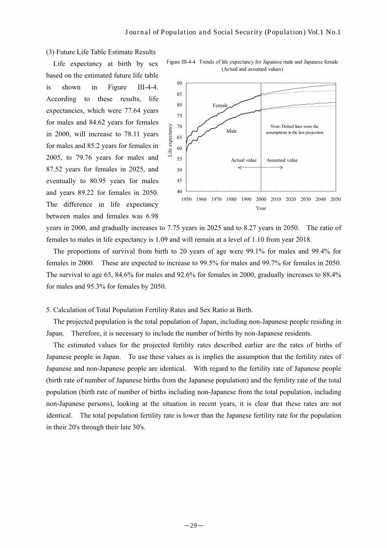
Journal of Population and Social Security (Population) Vol.1 No.1 (3) Future Life Table Estimate Results

Life expectancy at birth by sex based on the estimated future life table is shown in Figure III-4-4. According to these results, life expectancies, which were 77.64 years for males and 84.62 years for females in 2000, will increase to 78.11 years for males and 85.2 years for females in 2005, to 79.76 years for males and 87.52 years for females in 2025, and eventually to 80.95 years for males and years 89.22 for females in 2050. The difference in life expectancy between males and females was 6.98 years in 2000, and gradually increases to 7.75 years in 2025 and to 8.27 years in 2050. The ratio of females to males in life expectancy is 1.09 and will remain at a level of 1.10 from year 2018.

40

45

50

55

60

65

70

75

80

85

90

1950 1960 1970 1980 1990 2000 2010 2020 2030 2040 2050

Year

Life

exp

ecta

ncy

Male

Female

Actual value Assumed value

Note: Dotted lines were theassumptions in the last projection

Figure III-4-4　Trends of life expectancy for Japanese male and Japanese female(Actual and assumed values)

The proportions of survival from birth to 20 years of age were 99.1% for males and 99.4% for females in 2000. These are expected to increase to 99.5% for males and 99.7% for females in 2050. The survival to age 65, 84.6% for males and 92.6% for females in 2000, gradually increases to 88.4% for males and 95.3% for females by 2050. 5. Calculation of Total Population Fertility Rates and Sex Ratio at Birth.

The projected population is the total population of Japan, including non-Japanese people residing in Japan. Therefore, it is necessary to include the number of births by non-Japanese residents.

The estimated values for the projected fertility rates described earlier are the rates of births of Japanese people in Japan. To use these values as is implies the assumption that the fertility rates of Japanese and non-Japanese people are identical. With regard to the fertility rate of Japanese people (birth rate of number of Japanese births from the Japanese population) and the fertility rate of the total population (birth rate of number of births including non-Japanese from the total population, including non-Japanese persons), looking at the situation in recent years, it is clear that these rates are not identical. The total population fertility rate is lower than the Japanese fertility rate for the population in their 20's through their late 30's.

－29－

Journal of Population and Social Security (Population) Vol.1 No.1

Specifically, the ratio of the total population fertility and the Japanese population fertility for each age was determined, and the average of the values from 1990 to 2000 was defined as an adjustment factor for the calculation of the fertility rate of the total population. Then, this adjustment factor was multiplied by the estimated Japanese fertility rate to obtain a fertility rate for the total population. (Table III-5-1).

It is also necessary to estimate a sex ratio at birth (＝number of male births/number of female births × 100) in order to divide the future number of newborns into male and female. Based on observations of past sex ratio at birth, the fluctuations between years is negligible. Therefore, for this projection, it was assumed that the mean value (105.5) of the sex ratio at birth from 1996 to 2000 would also remain constant from 2001 onward (Figure III-5-1).

104

105

106

107

1985 1986 1987 1988 1989 1990 1991 1992 1993 1994 1995 1996 1997 1998 1999 2000

Year

Sex

ratio

at b

irth

(Fem

ale=

100)

Figure III-5-1　　Sex ratio at birth

6. International Migration Estimates

International migration has varied significantly ininternationalization and economic change. Furthermore, itas the economic and social situations in other countries. Tnet immigration to Japan, has not been stable over time However, if we separate the international migrations by Japthere is consistent net emigration by Japanese people, remyear since 1995. In comparison, there is generally a net im

－30－

Totalpopulation1) Only Japanese2)

15 0.00020 0.00020 1.0360316 0.00087 0.00085 1.0236917 0.00250 0.00247 1.0139818 0.00530 0.00526 1.0072519 0.01141 0.01137 1.0029820 0.01887 0.01888 1.0000121 0.02814 0.02820 0.9974222 0.03817 0.03833 0.9953723 0.05152 0.05186 0.9935724 0.06930 0.06987 0.9919425 0.08818 0.08902 0.9905526 0.10758 0.10872 0.9895227 0.12253 0.12392 0.9888228 0.13115 0.13268 0.9884229 0.13243 0.13399 0.9883930 0.12400 0.12543 0.9887531 0.11009 0.11126 0.9894532 0.09363 0.09453 0.9903933 0.07673 0.07738 0.9915134 0.06092 0.06137 0.99284

35 0.04628 0.04655 0.9943236 0.03429 0.03443 0.9958937 0.02382 0.02387 0.9974638 0.01624 0.01626 0.9990639 0.01081 0.01080 1.0004240 0.00673 0.00671 1.0015241 0.00399 0.00398 1.0025242 0.00220 0.00219 1.0031743 0.00116 0.00116 1.0039544 0.00056 0.00056 1.0069445 0.00024 0.00024 1.0110746 0.00009 0.00009 1.0174047 0.00004 0.00004 1.0277548 0.00001 0.00001 1.0434949 0.00001 0.00001 1.06432

2) Japanese fertility rate＝Live births of Japanese／Japanese population3) Adjustment＝Total population fertility rate／Japanese fertility rate 　Average of the values of 1990-2000（Greville's method of smoothing）

Age Adjustment3)

Average of age-specificfertility rate 1990-2000

1) Total population fertility rate＝Live births included non-Japanese ／Total population

Table III-5-1　　Adjustment for the totalpopulation fertility rate

Japan along with the progress of is affected by government policy as well he tendency in recent years, based on the and does not reveal any specific trend.

anese people and by non-Japanese people, aining relatively stable at about 40,000 a

migration to Japan among non-Japanese

Journal of Population and Social Security (Population) Vol.1 No.1 people, and although this varies a great deal, in recent years there is an apparent increasing trend.

The estimates for international migration for previous population projections used constant values for net immigration rates by age and sex. However, there are differences in the international migration trends shown by Japanese and non-Japanese people. In addition, population migration, particularly the number of immigrants, does not depend on the population size or composition. Therefore, the conventional method of using sex/age-specific immigration rates cannot be used to explain the current changes.

Here, we make separate assumptions regarding future international migration of Japanese and non-Japanese people. In other words, there will be 2 estimates; one for the net immigration of Japanese people, and another for the net immigration of non-Japanese people.

The international migration of Japanese people is relatively stable. Based on the net emigration (from Japan), the estimate is made as follows. First, the average of the values for the gross migration rates (net immigration rate) by age and sex between 1995 and 2000 are determined. Then, to eliminate the effect of coincidental changes, the adjusted rate is assumed to be constant from 2001 onward. (Figure III-6-1). Since the base value (population) for the number of migrations is the population of Japanese people, it is necessary to separately project the Japanese population. The proportion of the calculated future sex/age-specific

population that is Japanese (age-specific population: 2000 National Census; births: 2000 Vital Statistics) is used to determine the population of Japanese people.

(1)Male

-0.006

-0.005

-0.004

-0.003

-0.002

-0.001

0.000

0.001

0.002

0 10 20 30 40 50 60 70 80 90

1995-2000 AverageAssumption

(2)Female

-0.006

-0.005

-0.004

-0.003

-0.002

-0.001

0.000

0.001

0.002

0 10 20 30 40 50 60 70 80 90

1995-2000 AverageAssumption

Figure III-6-1　　Assumption of net (entries minus exits)international migration rate for Japanese population

Next, for the international migrations of non-Japanese people, there is generally a net immigration into Japan. Since there is an increasing trend in recent years, regression lines were fitted for each sex

－31－

Journal of Population and Social Security (Population) Vol.1 No.1

－32－

for the data since 1970. However, around 1990 there were drastic changes, so the data from the years between 1988 and 1995 was omitted because of the large discontinuity with the overall trend. By performing extrapolation with a logistics curve, the future sex-specific net immigration of non-Japanese people was determined. (Figure III-6-2). The proportion of each age of immigrants is taken to be constant, as the average of the values between 1995 and 2000. (Figure III-6-3).

Figure III-6-2　　Assumption of the amount of net (entries minus

exits) international migrants for non-Japanese population

1990 1995 2000 2005 2010 2015 2020 2025Year

-10

0

10

20

30

40

50

60

1970 1975 1980 1985

Exce

ss n

umbe

r of t

he e

ntry

Male

Female

(thousand)

-0.02

0.00

0.02

0.04

0.06

0.08

0.10

0 10 20 30 40 50 60 70 80 90Age

Exce

ss ra

te

Male

Female

Figure III-6-3　　Assumption of the age pattern of netinternational migration for non-Japanese population

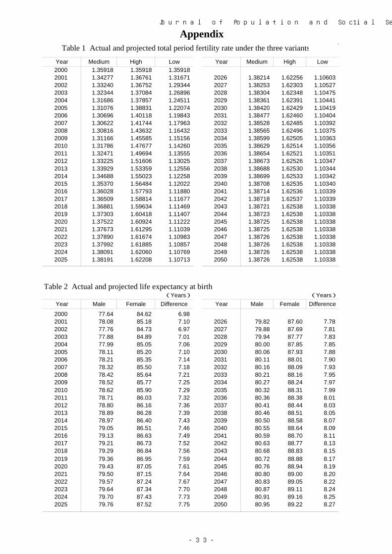
Journal of Population and Social Security (Population) Vol.1 No.1

Year Medium High Low Year Medium High Low2000 1.35918 1.35918 1.359182001 1.34277 1.36761 1.31671 2026 1.38214 1.62256 1.106032002 1.33240 1.36752 1.29344 2027 1.38253 1.62303 1.105272003 1.32344 1.37084 1.26896 2028 1.38304 1.62348 1.104752004 1.31686 1.37857 1.24511 2029 1.38361 1.62391 1.104412005 1.31076 1.38831 1.22074 2030 1.38420 1.62429 1.104192006 1.30696 1.40118 1.19843 2031 1.38477 1.62460 1.104042007 1.30622 1.41744 1.17963 2032 1.38528 1.62485 1.103922008 1.30816 1.43632 1.16432 2033 1.38565 1.62496 1.103752009 1.31166 1.45585 1.15156 2034 1.38599 1.62505 1.103632010 1.31786 1.47677 1.14260 2035 1.38629 1.62514 1.103562011 1.32471 1.49694 1.13555 2036 1.38654 1.62521 1.103512012 1.33225 1.51606 1.13025 2037 1.38673 1.62526 1.103472013 1.33929 1.53359 1.12556 2038 1.38688 1.62530 1.103442014 1.34688 1.55023 1.12258 2039 1.38699 1.62533 1.103422015 1.35370 1.56484 1.12022 2040 1.38708 1.62535 1.103402016 1.36028 1.57793 1.11880 2041 1.38714 1.62536 1.103392017 1.36509 1.58814 1.11677 2042 1.38718 1.62537 1.103392018 1.36881 1.59634 1.11469 2043 1.38721 1.62538 1.103382019 1.37303 1.60418 1.11407 2044 1.38723 1.62538 1.103382020 1.37522 1.60924 1.11222 2045 1.38725 1.62538 1.103382021 1.37673 1.61295 1.11039 2046 1.38725 1.62538 1.103382022 1.37890 1.61674 1.10983 2047 1.38726 1.62538 1.103382023 1.37992 1.61885 1.10857 2048 1.38726 1.62538 1.103382024 1.38091 1.62060 1.10769 2049 1.38726 1.62538 1.103382025 1.38191 1.62208 1.10713 2050 1.38726 1.62538 1.10338

（Years） （Years）Year Male Female Difference Year Male Female Difference2000 77.64 84.62 6.982001 78.08 85.18 7.10 2026 79.82 87.60 7.782002 77.76 84.73 6.97 2027 79.88 87.69 7.812003 77.88 84.89 7.01 2028 79.94 87.77 7.832004 77.99 85.05 7.06 2029 80.00 87.85 7.852005 78.11 85.20 7.10 2030 80.06 87.93 7.882006 78.21 85.35 7.14 2031 80.11 88.01 7.902007 78.32 85.50 7.18 2032 80.16 88.09 7.932008 78.42 85.64 7.21 2033 80.21 88.16 7.952009 78.52 85.77 7.25 2034 80.27 88.24 7.972010 78.62 85.90 7.29 2035 80.32 88.31 7.992011 78.71 86.03 7.32 2036 80.36 88.38 8.012012 78.80 86.16 7.36 2037 80.41 88.44 8.032013 78.89 86.28 7.39 2038 80.46 88.51 8.052014 78.97 86.40 7.43 2039 80.50 88.58 8.072015 79.05 86.51 7.46 2040 80.55 88.64 8.092016 79.13 86.63 7.49 2041 80.59 88.70 8.112017 79.21 86.73 7.52 2042 80.63 88.77 8.132018 79.29 86.84 7.56 2043 80.68 88.83 8.152019 79.36 86.95 7.59 2044 80.72 88.88 8.172020 79.43 87.05 7.61 2045 80.76 88.94 8.192021 79.50 87.15 7.64 2046 80.80 89.00 8.202022 79.57 87.24 7.67 2047 80.83 89.05 8.222023 79.64 87.34 7.70 2048 80.87 89.11 8.242024 79.70 87.43 7.73 2049 80.91 89.16 8.252025 79.76 87.52 7.75 2050 80.95 89.22 8.27

Table 1 Actual and projected total period fertility rate under the three variants

Appendix

Table 2 Actual and projected life expectancy at birth

-33-

Journal of Population and Social Security (Population) Vol.1 No.1

Table 3 　Projected future population and proportion by age group, 2000-2050: Medium variant

Total 0-14 15-64 65+ 0-14- 15-64- 65+

2000 126,926 18,505 86,380 22,041 14.6 68.1 17.42001 127,183 18,307 86,033 22,843 14.4 67.6 18.02002 127,377 18,123 85,673 23,581 14.2 67.3 18.52003 127,524 17,964 85,341 24,219 14.1 66.9 19.02004 127,635 17,842 85,071 24,722 14.0 66.7 19.4

2005 127,708 17,727 84,590 25,392 13.9 66.2 19.92006 127,741 17,623 83,946 26,172 13.8 65.7 20.52007 127,733 17,501 83,272 26,959 13.7 65.2 21.12008 127,686 17,385 82,643 27,658 13.6 64.7 21.72009 127,599 17,235 81,994 28,370 13.5 64.3 22.2

2010 127,473 17,074 81,665 28,735 13.4 64.1 22.52011 127,309 16,919 81,422 28,968 13.3 64.0 22.82012 127,107 16,746 80,418 29,942 13.2 63.3 23.62013 126,865 16,558 79,326 30,981 13.1 62.5 24.42014 126,585 16,385 78,207 31,992 12.9 61.8 25.3

2015 126,266 16,197 77,296 32,772 12.8 61.2 26.02016 125,909 15,980 76,556 33,372 12.7 60.8 26.52017 125,513 15,759 75,921 33,832 12.6 60.5 27.02018 125,080 15,536 75,374 34,170 12.4 60.3 27.32019 124,611 15,314 74,918 34,379 12.3 60.1 27.6

2020 124,107 15,095 74,453 34,559 12.2 60.0 27.82021 123,570 14,881 74,026 34,663 12.0 59.9 28.12022 123,002 14,673 73,658 34,671 11.9 59.9 28.22023 122,406 14,471 73,242 34,694 11.8 59.8 28.32024 121,784 14,275 72,775 34,734 11.7 59.8 28.5

2025 121,136 14,085 72,325 34,726 11.6 59.7 28.72026 120,466 13,901 71,877 34,688 11.5 59.7 28.82027 119,773 13,724 71,397 34,652 11.5 59.6 28.92028 119,061 13,553 70,858 34,650 11.4 59.5 29.12029 118,329 13,389 70,275 34,665 11.3 59.4 29.3

2030 117,580 13,233 69,576 34,770 11.3 59.2 29.62031 116,813 13,085 69,174 34,554 11.2 59.2 29.62032 116,032 12,944 68,398 34,689 11.2 58.9 29.92033 115,235 12,812 67,608 34,815 11.1 58.7 30.22034 114,425 12,686 66,771 34,968 11.1 58.4 30.6

2035 113,602 12,567 65,891 35,145 11.1 58.0 30.92036 112,768 12,453 64,953 35,362 11.0 57.6 31.42037 111,923 12,341 63,962 35,619 11.0 57.1 31.82038 111,068 12,233 62,928 35,908 11.0 56.7 32.32039 110,207 12,125 61,919 36,163 11.0 56.2 32.8

2040 109,338 12,017 60,990 36,332 11.0 55.8 33.22041 108,465 11,908 60,126 36,432 11.0 55.4 33.62042 107,589 11,798 59,329 36,462 11.0 55.1 33.92043 106,712 11,686 58,555 36,471 11.0 54.9 34.22044 105,835 11,572 57,824 36,439 10.9 54.6 34.4

2045 104,960 11,455 57,108 36,396 10.9 54.4 34.72046 104,087 11,336 56,449 36,302 10.9 54.2 34.92047 103,213 11,215 55,800 36,198 10.9 54.1 35.12048 102,339 11,092 55,146 36,102 10.8 53.9 35.32049 101,466 10,967 54,498 36,001 10.8 53.7 35.5

2050 100,593 10,842 53,889 35,863 10.8 53.6 35.7

YearPopulation（thousand） Proportion（%）

-34-

Journal of Population and Social Security (Population) Vol.1 No.1

Table 4 　Projected future population and proportion by age group, 2000-2050: High variant

Total 0-14 15-64 65+ 0-14- 15-64- 65+

2000 126,926 18,505 86,380 22,041 14.6 68.1 17.42001 127,198 18,322 86,033 22,843 14.4 67.6 18.02002 127,419 18,165 85,673 23,581 14.3 67.2 18.52003 127,603 18,043 85,341 24,219 14.1 66.9 19.02004 127,762 17,969 85,071 24,722 14.1 66.6 19.4

2005 127,894 17,913 84,590 25,392 14.0 66.1 19.92006 128,000 17,882 83,946 26,172 14.0 65.6 20.42007 128,078 17,846 83,272 26,959 13.9 65.0 21.02008 128,128 17,828 82,643 27,658 13.9 64.5 21.62009 128,151 17,787 81,994 28,370 13.9 64.0 22.1

2010 128,145 17,746 81,665 28,735 13.8 63.7 22.42011 128,110 17,720 81,422 28,968 13.8 63.6 22.62012 128,043 17,683 80,418 29,942 13.8 62.8 23.42013 127,943 17,636 79,326 30,981 13.8 62.0 24.22014 127,809 17,609 78,207 31,992 13.8 61.2 25.0

2015 127,640 17,571 77,296 32,772 13.8 60.6 25.72016 127,435 17,491 76,571 33,372 13.7 60.1 26.22017 127,193 17,398 75,963 33,832 13.7 59.7 26.62018 126,914 17,293 75,452 34,170 13.6 59.5 26.92019 126,600 17,178 75,043 34,379 13.6 59.3 27.2

2020 126,250 17,053 74,638 34,559 13.5 59.1 27.42021 125,867 16,921 74,284 34,663 13.4 59.0 27.52022 125,453 16,781 74,001 34,671 13.4 59.0 27.62023 125,010 16,634 73,682 34,694 13.3 58.9 27.82024 124,539 16,481 73,325 34,734 13.2 58.9 27.9

2025 124,044 16,325 72,993 34,726 13.2 58.8 28.02026 123,526 16,166 72,673 34,688 13.1 58.8 28.12027 122,987 16,006 72,328 34,652 13.0 58.8 28.22028 122,428 15,849 71,929 34,650 12.9 58.8 28.32029 121,853 15,696 71,491 34,665 12.9 58.7 28.4

2030 121,262 15,550 70,941 34,770 12.8 58.5 28.72031 120,657 15,412 70,691 34,554 12.8 58.6 28.62032 120,039 15,284 70,067 34,689 12.7 58.4 28.92033 119,411 15,167 69,429 34,815 12.7 58.1 29.22034 118,774 15,061 68,746 34,968 12.7 57.9 29.4

2035 118,129 14,966 68,018 35,145 12.7 57.6 29.82036 117,477 14,882 67,233 35,362 12.7 57.2 30.12037 116,819 14,806 66,394 35,619 12.7 56.8 30.52038 116,156 14,738 65,511 35,908 12.7 56.4 30.92039 115,491 14,676 64,652 36,163 12.7 56.0 31.3

2040 114,824 14,619 63,874 36,332 12.7 55.6 31.62041 114,157 14,565 63,160 36,432 12.8 55.3 31.92042 113,490 14,512 62,515 36,462 12.8 55.1 32.12043 112,825 14,460 61,894 36,471 12.8 54.9 32.32044 112,163 14,407 61,317 36,439 12.8 54.7 32.5

2045 111,506 14,351 60,758 36,396 12.9 54.5 32.62046 110,852 14,291 60,258 36,302 12.9 54.4 32.72047 110,198 14,228 59,773 36,198 12.9 54.2 32.82048 109,546 14,159 59,285 36,102 12.9 54.1 33.02049 108,895 14,086 58,809 36,001 12.9 54.0 33.1

2050 108,246 14,008 58,375 35,863 12.9 53.9 33.1

YearPopulation（thousand） Proportion（%）

-35-

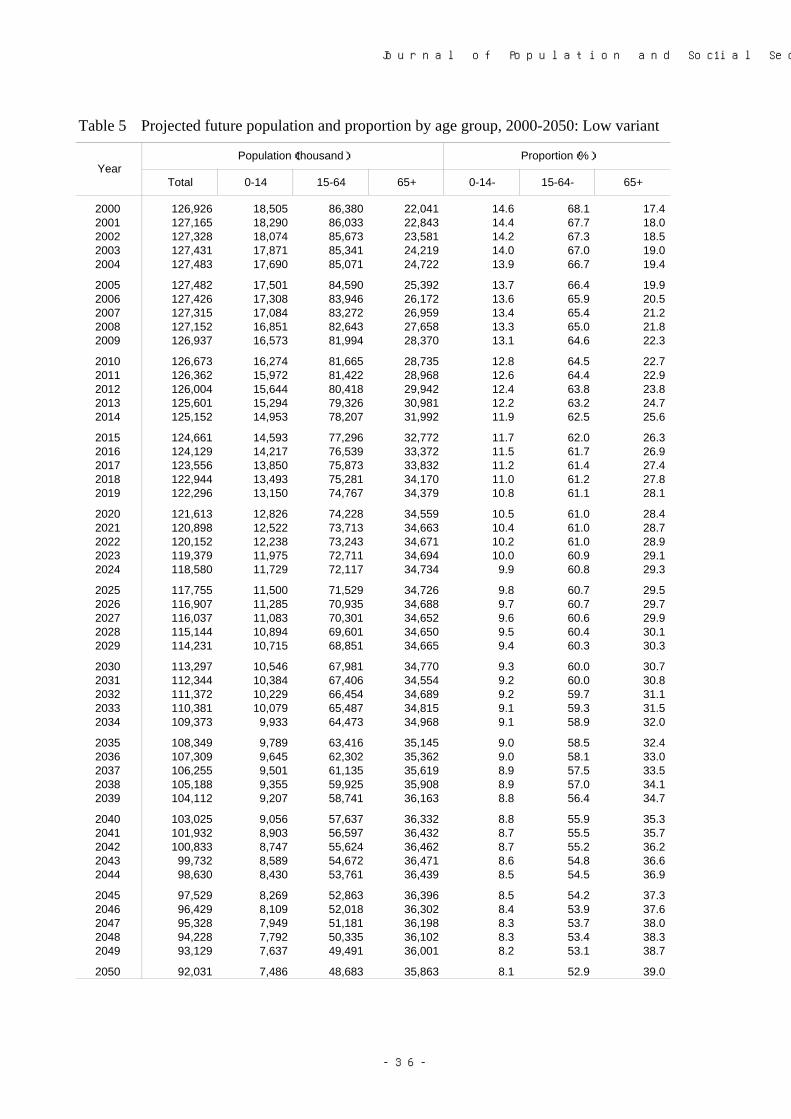
Journal of Population and Social Security (Population) Vol.1 No.1

Table 5 　Projected future population and proportion by age group, 2000-2050: Low variant

Total 0-14 15-64 65+ 0-14- 15-64- 65+

2000 126,926 18,505 86,380 22,041 14.6 68.1 17.42001 127,165 18,290 86,033 22,843 14.4 67.7 18.02002 127,328 18,074 85,673 23,581 14.2 67.3 18.52003 127,431 17,871 85,341 24,219 14.0 67.0 19.02004 127,483 17,690 85,071 24,722 13.9 66.7 19.4

2005 127,482 17,501 84,590 25,392 13.7 66.4 19.92006 127,426 17,308 83,946 26,172 13.6 65.9 20.52007 127,315 17,084 83,272 26,959 13.4 65.4 21.22008 127,152 16,851 82,643 27,658 13.3 65.0 21.82009 126,937 16,573 81,994 28,370 13.1 64.6 22.3

2010 126,673 16,274 81,665 28,735 12.8 64.5 22.72011 126,362 15,972 81,422 28,968 12.6 64.4 22.92012 126,004 15,644 80,418 29,942 12.4 63.8 23.82013 125,601 15,294 79,326 30,981 12.2 63.2 24.72014 125,152 14,953 78,207 31,992 11.9 62.5 25.6

2015 124,661 14,593 77,296 32,772 11.7 62.0 26.32016 124,129 14,217 76,539 33,372 11.5 61.7 26.92017 123,556 13,850 75,873 33,832 11.2 61.4 27.42018 122,944 13,493 75,281 34,170 11.0 61.2 27.82019 122,296 13,150 74,767 34,379 10.8 61.1 28.1

2020 121,613 12,826 74,228 34,559 10.5 61.0 28.42021 120,898 12,522 73,713 34,663 10.4 61.0 28.72022 120,152 12,238 73,243 34,671 10.2 61.0 28.92023 119,379 11,975 72,711 34,694 10.0 60.9 29.12024 118,580 11,729 72,117 34,734 9.9 60.8 29.3

2025 117,755 11,500 71,529 34,726 9.8 60.7 29.52026 116,907 11,285 70,935 34,688 9.7 60.7 29.72027 116,037 11,083 70,301 34,652 9.6 60.6 29.92028 115,144 10,894 69,601 34,650 9.5 60.4 30.12029 114,231 10,715 68,851 34,665 9.4 60.3 30.3

2030 113,297 10,546 67,981 34,770 9.3 60.0 30.72031 112,344 10,384 67,406 34,554 9.2 60.0 30.82032 111,372 10,229 66,454 34,689 9.2 59.7 31.12033 110,381 10,079 65,487 34,815 9.1 59.3 31.52034 109,373 9,933 64,473 34,968 9.1 58.9 32.0

2035 108,349 9,789 63,416 35,145 9.0 58.5 32.42036 107,309 9,645 62,302 35,362 9.0 58.1 33.02037 106,255 9,501 61,135 35,619 8.9 57.5 33.52038 105,188 9,355 59,925 35,908 8.9 57.0 34.12039 104,112 9,207 58,741 36,163 8.8 56.4 34.7

2040 103,025 9,056 57,637 36,332 8.8 55.9 35.32041 101,932 8,903 56,597 36,432 8.7 55.5 35.72042 100,833 8,747 55,624 36,462 8.7 55.2 36.22043 99,732 8,589 54,672 36,471 8.6 54.8 36.62044 98,630 8,430 53,761 36,439 8.5 54.5 36.9

2045 97,529 8,269 52,863 36,396 8.5 54.2 37.32046 96,429 8,109 52,018 36,302 8.4 53.9 37.62047 95,328 7,949 51,181 36,198 8.3 53.7 38.02048 94,228 7,792 50,335 36,102 8.3 53.4 38.32049 93,129 7,637 49,491 36,001 8.2 53.1 38.7

2050 92,031 7,486 48,683 35,863 8.1 52.9 39.0

YearPopulation（thousand） Proportion（%）

-36-

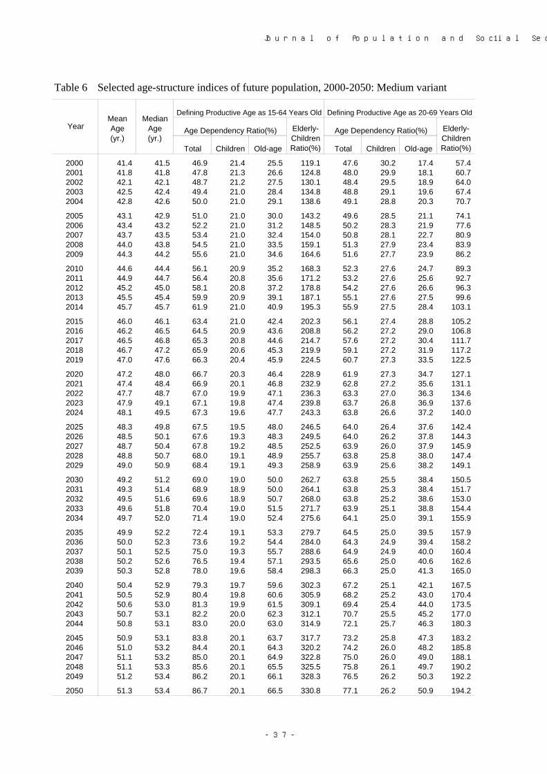
Journal of Population and Social Security (Population) Vol.1 No.1

Table 6 　Selected age-structure indices of future population, 2000-2050: Medium variant

Total Children Old-age Total Children Old-age

2000 41.4 41.5 46.9 21.4 25.5 119.1 47.6 30.2 17.4 57.42001 41.8 41.8 47.8 21.3 26.6 124.8 48.0 29.9 18.1 60.72002 42.1 42.1 48.7 21.2 27.5 130.1 48.4 29.5 18.9 64.02003 42.5 42.4 49.4 21.0 28.4 134.8 48.8 29.1 19.6 67.42004 42.8 42.6 50.0 21.0 29.1 138.6 49.1 28.8 20.3 70.7

2005 43.1 42.9 51.0 21.0 30.0 143.2 49.6 28.5 21.1 74.12006 43.4 43.2 52.2 21.0 31.2 148.5 50.2 28.3 21.9 77.62007 43.7 43.5 53.4 21.0 32.4 154.0 50.8 28.1 22.7 80.92008 44.0 43.8 54.5 21.0 33.5 159.1 51.3 27.9 23.4 83.92009 44.3 44.2 55.6 21.0 34.6 164.6 51.6 27.7 23.9 86.2

2010 44.6 44.4 56.1 20.9 35.2 168.3 52.3 27.6 24.7 89.32011 44.9 44.7 56.4 20.8 35.6 171.2 53.2 27.6 25.6 92.72012 45.2 45.0 58.1 20.8 37.2 178.8 54.2 27.6 26.6 96.32013 45.5 45.4 59.9 20.9 39.1 187.1 55.1 27.6 27.5 99.62014 45.7 45.7 61.9 21.0 40.9 195.3 55.9 27.5 28.4 103.1

2015 46.0 46.1 63.4 21.0 42.4 202.3 56.1 27.4 28.8 105.22016 46.2 46.5 64.5 20.9 43.6 208.8 56.2 27.2 29.0 106.82017 46.5 46.8 65.3 20.8 44.6 214.7 57.6 27.2 30.4 111.72018 46.7 47.2 65.9 20.6 45.3 219.9 59.1 27.2 31.9 117.22019 47.0 47.6 66.3 20.4 45.9 224.5 60.7 27.3 33.5 122.5

2020 47.2 48.0 66.7 20.3 46.4 228.9 61.9 27.3 34.7 127.12021 47.4 48.4 66.9 20.1 46.8 232.9 62.8 27.2 35.6 131.12022 47.7 48.7 67.0 19.9 47.1 236.3 63.3 27.0 36.3 134.62023 47.9 49.1 67.1 19.8 47.4 239.8 63.7 26.8 36.9 137.62024 48.1 49.5 67.3 19.6 47.7 243.3 63.8 26.6 37.2 140.0

2025 48.3 49.8 67.5 19.5 48.0 246.5 64.0 26.4 37.6 142.42026 48.5 50.1 67.6 19.3 48.3 249.5 64.0 26.2 37.8 144.32027 48.7 50.4 67.8 19.2 48.5 252.5 63.9 26.0 37.9 145.92028 48.8 50.7 68.0 19.1 48.9 255.7 63.8 25.8 38.0 147.42029 49.0 50.9 68.4 19.1 49.3 258.9 63.9 25.6 38.2 149.1

2030 49.2 51.2 69.0 19.0 50.0 262.7 63.8 25.5 38.4 150.52031 49.3 51.4 68.9 18.9 50.0 264.1 63.8 25.3 38.4 151.72032 49.5 51.6 69.6 18.9 50.7 268.0 63.8 25.2 38.6 153.02033 49.6 51.8 70.4 19.0 51.5 271.7 63.9 25.1 38.8 154.42034 49.7 52.0 71.4 19.0 52.4 275.6 64.1 25.0 39.1 155.9

2035 49.9 52.2 72.4 19.1 53.3 279.7 64.5 25.0 39.5 157.92036 50.0 52.3 73.6 19.2 54.4 284.0 64.3 24.9 39.4 158.22037 50.1 52.5 75.0 19.3 55.7 288.6 64.9 24.9 40.0 160.42038 50.2 52.6 76.5 19.4 57.1 293.5 65.6 25.0 40.6 162.62039 50.3 52.8 78.0 19.6 58.4 298.3 66.3 25.0 41.3 165.0

2040 50.4 52.9 79.3 19.7 59.6 302.3 67.2 25.1 42.1 167.52041 50.5 52.9 80.4 19.8 60.6 305.9 68.2 25.2 43.0 170.42042 50.6 53.0 81.3 19.9 61.5 309.1 69.4 25.4 44.0 173.52043 50.7 53.1 82.2 20.0 62.3 312.1 70.7 25.5 45.2 177.02044 50.8 53.1 83.0 20.0 63.0 314.9 72.1 25.7 46.3 180.3

2045 50.9 53.1 83.8 20.1 63.7 317.7 73.2 25.8 47.3 183.22046 51.0 53.2 84.4 20.1 64.3 320.2 74.2 26.0 48.2 185.82047 51.1 53.2 85.0 20.1 64.9 322.8 75.0 26.0 49.0 188.12048 51.1 53.3 85.6 20.1 65.5 325.5 75.8 26.1 49.7 190.22049 51.2 53.4 86.2 20.1 66.1 328.3 76.5 26.2 50.3 192.2

2050 51.3 53.4 86.7 20.1 66.5 330.8 77.1 26.2 50.9 194.2

Defining Productive Age as 20-69 Years Old

Age Dependency Ratio(%) Elderly-ChildrenRatio(%)

YearMeanAge(yr.)

MedianAge(yr.)

Defining Productive Age as 15-64 Years Old

Age Dependency Ratio(%) Elderly-ChildrenRatio(%)

-37-

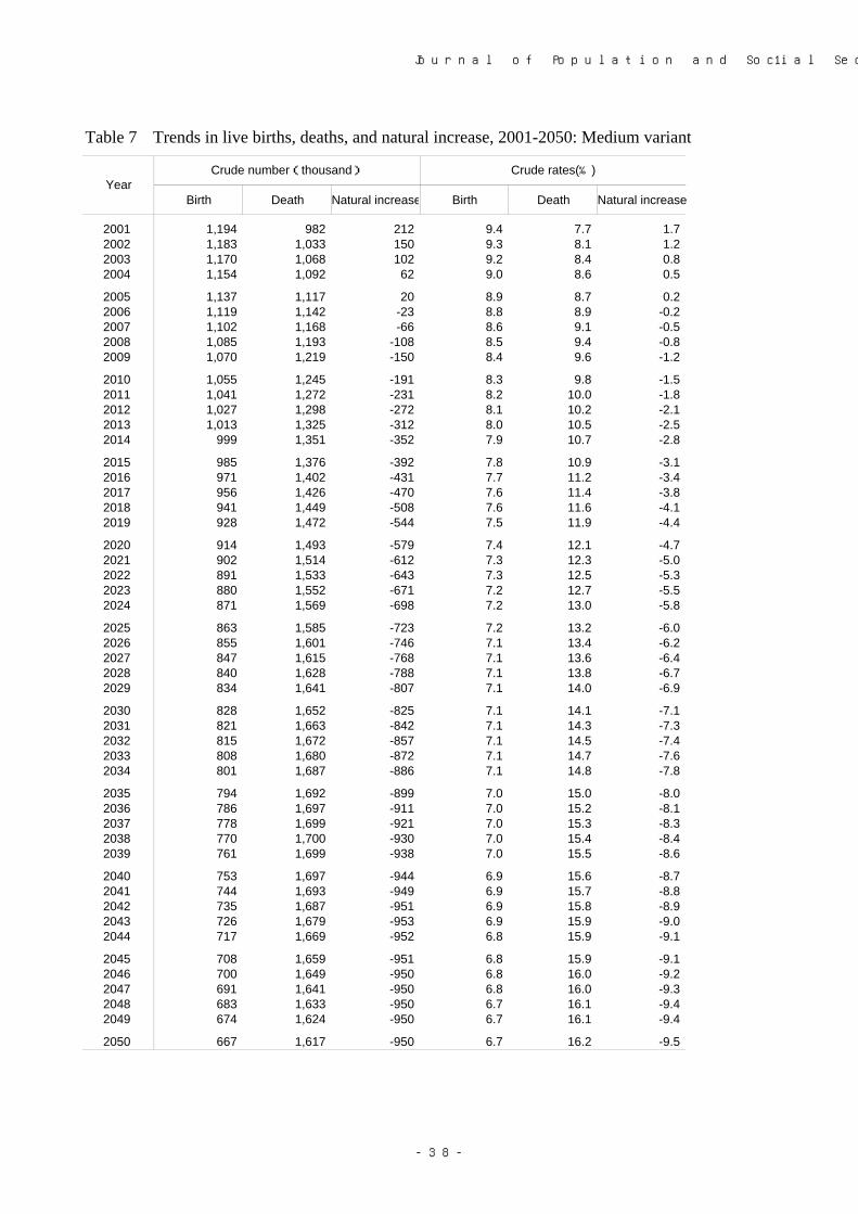
Journal of Population and Social Security (Population) Vol.1 No.1

Table 7 　Trends in live births, deaths, and natural increase, 2001-2050: Medium variant

Birth Death Natural increase Birth Death Natural increase

2001 1,194 982 212 9.4 7.7 1.72002 1,183 1,033 150 9.3 8.1 1.22003 1,170 1,068 102 9.2 8.4 0.82004 1,154 1,092 62 9.0 8.6 0.5

2005 1,137 1,117 20 8.9 8.7 0.22006 1,119 1,142 -23 8.8 8.9 -0.22007 1,102 1,168 -66 8.6 9.1 -0.52008 1,085 1,193 -108 8.5 9.4 -0.82009 1,070 1,219 -150 8.4 9.6 -1.2

2010 1,055 1,245 -191 8.3 9.8 -1.52011 1,041 1,272 -231 8.2 10.0 -1.82012 1,027 1,298 -272 8.1 10.2 -2.12013 1,013 1,325 -312 8.0 10.5 -2.52014 999 1,351 -352 7.9 10.7 -2.8

2015 985 1,376 -392 7.8 10.9 -3.12016 971 1,402 -431 7.7 11.2 -3.42017 956 1,426 -470 7.6 11.4 -3.82018 941 1,449 -508 7.6 11.6 -4.12019 928 1,472 -544 7.5 11.9 -4.4

2020 914 1,493 -579 7.4 12.1 -4.72021 902 1,514 -612 7.3 12.3 -5.02022 891 1,533 -643 7.3 12.5 -5.32023 880 1,552 -671 7.2 12.7 -5.52024 871 1,569 -698 7.2 13.0 -5.8

2025 863 1,585 -723 7.2 13.2 -6.02026 855 1,601 -746 7.1 13.4 -6.22027 847 1,615 -768 7.1 13.6 -6.42028 840 1,628 -788 7.1 13.8 -6.72029 834 1,641 -807 7.1 14.0 -6.9

2030 828 1,652 -825 7.1 14.1 -7.12031 821 1,663 -842 7.1 14.3 -7.32032 815 1,672 -857 7.1 14.5 -7.42033 808 1,680 -872 7.1 14.7 -7.62034 801 1,687 -886 7.1 14.8 -7.8

2035 794 1,692 -899 7.0 15.0 -8.02036 786 1,697 -911 7.0 15.2 -8.12037 778 1,699 -921 7.0 15.3 -8.32038 770 1,700 -930 7.0 15.4 -8.42039 761 1,699 -938 7.0 15.5 -8.6

2040 753 1,697 -944 6.9 15.6 -8.72041 744 1,693 -949 6.9 15.7 -8.82042 735 1,687 -951 6.9 15.8 -8.92043 726 1,679 -953 6.9 15.9 -9.02044 717 1,669 -952 6.8 15.9 -9.1

2045 708 1,659 -951 6.8 15.9 -9.12046 700 1,649 -950 6.8 16.0 -9.22047 691 1,641 -950 6.8 16.0 -9.32048 683 1,633 -950 6.7 16.1 -9.42049 674 1,624 -950 6.7 16.1 -9.4

2050 667 1,617 -950 6.7 16.2 -9.5

YearCrude number（thousand） Crude rates(‰)

-38-

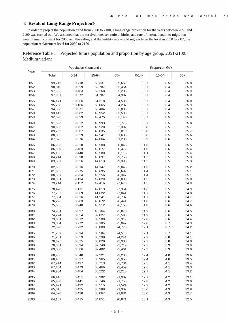
Journal of Population and Social Security (Population) Vol.1 No.1

≪Result of Long-Range Projection≫

Total 0-14 15-64 65+ 0-14- 15-64- 65+

2051 99,719 10,718 53,331 35,669 10.7 53.5 35.82052 98,840 10,599 52,787 35,454 10.7 53.4 35.92053 97,956 10,483 52,268 35,205 10.7 53.4 35.92054 97,067 10,372 51,787 34,907 10.7 53.4 36.0

2055 96,171 10,266 51,318 34,586 10.7 53.4 36.02056 95,268 10,166 50,865 34,237 10.7 53.4 35.92057 94,358 10,071 50,404 33,883 10.7 53.4 35.92058 93,442 9,982 49,952 33,508 10.7 53.5 35.92059 92,520 9,899 49,475 33,146 10.7 53.5 35.8

2060 91,593 9,822 48,993 32,778 10.7 53.5 35.82061 90,663 9,752 48,520 32,392 10.8 53.5 35.72062 89,732 9,687 48,035 32,010 10.8 53.5 35.72063 88,802 9,629 47,541 31,633 10.8 53.5 35.62064 87,875 9,576 47,064 31,235 10.9 53.6 35.5

2065 86,953 9,528 46,580 30,845 11.0 53.6 35.52066 86,039 9,483 46,077 30,479 11.0 53.6 35.42067 85,136 9,440 45,580 30,116 11.1 53.5 35.42068 84,244 9,398 45,091 29,755 11.2 53.5 35.32069 83,367 9,356 44,613 29,398 11.2 53.5 35.3

2070 82,506 9,316 44,147 29,043 11.3 53.5 35.22071 81,662 9,275 43,695 28,692 11.4 53.5 35.12072 80,837 9,234 43,256 28,347 11.4 53.5 35.12073 80,031 9,194 42,829 28,008 11.5 53.5 35.02074 79,244 9,152 42,416 27,676 11.5 53.5 34.9

2075 78,478 9,111 42,013 27,354 11.6 53.5 34.92076 77,732 9,069 41,622 27,041 11.7 53.5 34.82077 77,004 9,026 41,241 26,737 11.7 53.6 34.72078 76,296 8,983 40,872 26,441 11.8 53.6 34.72079 75,605 8,940 40,512 26,153 11.8 53.6 34.6

2080 74,931 8,897 40,164 25,870 11.9 53.6 34.52081 74,274 8,854 39,827 25,593 11.9 53.6 34.52082 73,631 8,812 39,500 25,319 12.0 53.6 34.42083 73,004 8,772 39,185 25,047 12.0 53.7 34.32084 72,390 8,732 38,880 24,778 12.1 53.7 34.2

2085 71,789 8,694 38,584 24,510 12.1 53.7 34.12086 71,201 8,659 38,298 24,244 12.2 53.8 34.12087 70,625 8,625 38,020 23,980 12.2 53.8 34.02088 70,061 8,594 37,748 23,719 12.3 53.9 33.92089 69,508 8,566 37,482 23,461 12.3 53.9 33.8

2090 68,966 8,540 37,221 23,205 12.4 54.0 33.62091 68,435 8,517 36,965 22,953 12.4 54.0 33.52092 67,914 8,497 36,713 22,704 12.5 54.1 33.42093 67,404 8,479 36,466 22,459 12.6 54.1 33.32094 66,904 8,464 36,222 22,218 12.7 54.1 33.2

2095 66,416 8,451 35,982 21,982 12.7 54.2 33.12096 65,938 8,441 35,746 21,750 12.8 54.2 33.02097 65,471 8,432 35,515 21,524 12.9 54.2 32.92098 65,015 8,425 35,288 21,302 13.0 54.3 32.82099 64,570 8,420 35,067 21,084 13.0 54.3 32.7

2100 64,137 8,415 34,851 20,871 13.1 54.3 32.5

　　In order to project the population trend from 2000 to 2100, a long-range projection for the years between 2051 and2100 was carried out. We assumed that the survival rate, sex ratio at births, and rate of international net-migrationwould remain constant for 2050 and thereafter, and the fertility rate would regress from the level in 2050 to 2.07, thepopulation replacement level for 2050 to 2150

YearPopulation（thousand） Proportion（%）

Reference Table 1 　Projected future population and proportion by age group, 2051-2100:Medium variant

-39-

Journal of Population and Social Security (Population) Vol.1 No.1

Total 0-14 15-64 65+ 0-14- 15-64- 65+

2051 107,593 13,926 57,997 35,669 12.9 53.9 33.22052 106,935 13,843 57,638 35,454 12.9 53.9 33.22053 106,271 13,757 57,309 35,205 12.9 53.9 33.12054 105,600 13,671 57,022 34,907 12.9 54.0 33.1

2055 104,922 13,585 56,751 34,586 12.9 54.1 33.02056 104,236 13,499 56,500 34,237 13.0 54.2 32.82057 103,542 13,414 56,245 33,883 13.0 54.3 32.72058 102,841 13,331 56,002 33,508 13.0 54.5 32.62059 102,133 13,252 55,736 33,146 13.0 54.6 32.5

2060 101,421 13,176 55,467 32,778 13.0 54.7 32.32061 100,705 13,105 55,208 32,392 13.0 54.8 32.22062 99,989 13,040 54,939 32,010 13.0 54.9 32.02063 99,273 12,980 54,661 31,633 13.1 55.1 31.92064 98,561 12,926 54,400 31,235 13.1 55.2 31.7

2065 97,854 12,878 54,132 30,845 13.2 55.3 31.52066 97,158 12,834 53,830 30,493 13.2 55.4 31.42067 96,471 12,795 53,523 30,154 13.3 55.5 31.32068 95,798 12,759 53,213 29,825 13.3 55.5 31.12069 95,139 12,727 52,903 29,510 13.4 55.6 31.0

2070 94,498 12,697 52,592 29,209 13.4 55.7 30.92071 93,874 12,670 52,282 28,922 13.5 55.7 30.82072 93,269 12,644 51,973 28,652 13.6 55.7 30.72073 92,684 12,620 51,665 28,398 13.6 55.7 30.62074 92,118 12,597 51,359 28,162 13.7 55.8 30.6

2075 91,572 12,574 51,055 27,943 13.7 55.8 30.52076 91,045 12,551 50,754 27,741 13.8 55.7 30.52077 90,537 12,527 50,457 27,552 13.8 55.7 30.42078 90,046 12,503 50,167 27,376 13.9 55.7 30.42079 89,571 12,477 49,884 27,209 13.9 55.7 30.4

2080 89,111 12,450 49,610 27,050 14.0 55.7 30.42081 88,664 12,423 49,346 26,896 14.0 55.7 30.32082 88,231 12,394 49,093 26,744 14.0 55.6 30.32083 87,809 12,364 48,852 26,594 14.1 55.6 30.32084 87,398 12,333 48,622 26,442 14.1 55.6 30.3

2085 86,996 12,302 48,404 26,290 14.1 55.6 30.22086 86,603 12,271 48,197 26,135 14.2 55.7 30.22087 86,219 12,240 47,999 25,980 14.2 55.7 30.12088 85,841 12,210 47,809 25,822 14.2 55.7 30.12089 85,471 12,181 47,627 25,663 14.3 55.7 30.0

2090 85,106 12,154 47,450 25,502 14.3 55.8 30.02091 84,748 12,128 47,279 25,341 14.3 55.8 29.92092 84,394 12,105 47,111 25,179 14.3 55.8 29.82093 84,047 12,083 46,947 25,016 14.4 55.9 29.82094 83,704 12,064 46,784 24,855 14.4 55.9 29.7

2095 83,366 12,048 46,623 24,695 14.5 55.9 29.62096 83,034 12,034 46,463 24,537 14.5 56.0 29.52097 82,708 12,023 46,304 24,381 14.5 56.0 29.52098 82,387 12,014 46,145 24,228 14.6 56.0 29.42099 82,072 12,008 45,986 24,078 14.6 56.0 29.3

2100 81,764 12,004 45,829 23,931 14.7 56.1 29.3

YearPopulation（thousand） Proportion（%）

Reference Table 2 　Projected future population and proportion by age group, 2051-2100:High variant

-40-

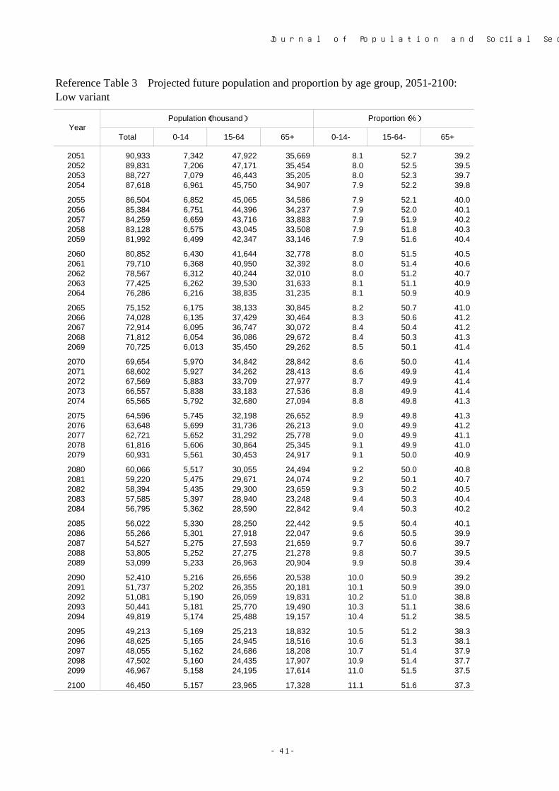
Journal of Population and Social Security (Population) Vol.1 No.1

Total 0-14 15-64 65+ 0-14- 15-64- 65+

2051 90,933 7,342 47,922 35,669 8.1 52.7 39.22052 89,831 7,206 47,171 35,454 8.0 52.5 39.52053 88,727 7,079 46,443 35,205 8.0 52.3 39.72054 87,618 6,961 45,750 34,907 7.9 52.2 39.8

2055 86,504 6,852 45,065 34,586 7.9 52.1 40.02056 85,384 6,751 44,396 34,237 7.9 52.0 40.12057 84,259 6,659 43,716 33,883 7.9 51.9 40.22058 83,128 6,575 43,045 33,508 7.9 51.8 40.32059 81,992 6,499 42,347 33,146 7.9 51.6 40.4

2060 80,852 6,430 41,644 32,778 8.0 51.5 40.52061 79,710 6,368 40,950 32,392 8.0 51.4 40.62062 78,567 6,312 40,244 32,010 8.0 51.2 40.72063 77,425 6,262 39,530 31,633 8.1 51.1 40.92064 76,286 6,216 38,835 31,235 8.1 50.9 40.9

2065 75,152 6,175 38,133 30,845 8.2 50.7 41.02066 74,028 6,135 37,429 30,464 8.3 50.6 41.22067 72,914 6,095 36,747 30,072 8.4 50.4 41.22068 71,812 6,054 36,086 29,672 8.4 50.3 41.32069 70,725 6,013 35,450 29,262 8.5 50.1 41.4

2070 69,654 5,970 34,842 28,842 8.6 50.0 41.42071 68,602 5,927 34,262 28,413 8.6 49.9 41.42072 67,569 5,883 33,709 27,977 8.7 49.9 41.42073 66,557 5,838 33,183 27,536 8.8 49.9 41.42074 65,565 5,792 32,680 27,094 8.8 49.8 41.3

2075 64,596 5,745 32,198 26,652 8.9 49.8 41.32076 63,648 5,699 31,736 26,213 9.0 49.9 41.22077 62,721 5,652 31,292 25,778 9.0 49.9 41.12078 61,816 5,606 30,864 25,345 9.1 49.9 41.02079 60,931 5,561 30,453 24,917 9.1 50.0 40.9

2080 60,066 5,517 30,055 24,494 9.2 50.0 40.82081 59,220 5,475 29,671 24,074 9.2 50.1 40.72082 58,394 5,435 29,300 23,659 9.3 50.2 40.52083 57,585 5,397 28,940 23,248 9.4 50.3 40.42084 56,795 5,362 28,590 22,842 9.4 50.3 40.2

2085 56,022 5,330 28,250 22,442 9.5 50.4 40.12086 55,266 5,301 27,918 22,047 9.6 50.5 39.92087 54,527 5,275 27,593 21,659 9.7 50.6 39.72088 53,805 5,252 27,275 21,278 9.8 50.7 39.52089 53,099 5,233 26,963 20,904 9.9 50.8 39.4

2090 52,410 5,216 26,656 20,538 10.0 50.9 39.22091 51,737 5,202 26,355 20,181 10.1 50.9 39.02092 51,081 5,190 26,059 19,831 10.2 51.0 38.82093 50,441 5,181 25,770 19,490 10.3 51.1 38.62094 49,819 5,174 25,488 19,157 10.4 51.2 38.5

2095 49,213 5,169 25,213 18,832 10.5 51.2 38.32096 48,625 5,165 24,945 18,516 10.6 51.3 38.12097 48,055 5,162 24,686 18,208 10.7 51.4 37.92098 47,502 5,160 24,435 17,907 10.9 51.4 37.72099 46,967 5,158 24,195 17,614 11.0 51.5 37.5

2100 46,450 5,157 23,965 17,328 11.1 51.6 37.3

YearPopulation（thousand） Proportion（%）

Reference Table 3 　Projected future population and proportion by age group, 2051-2100:Low variant

-41-

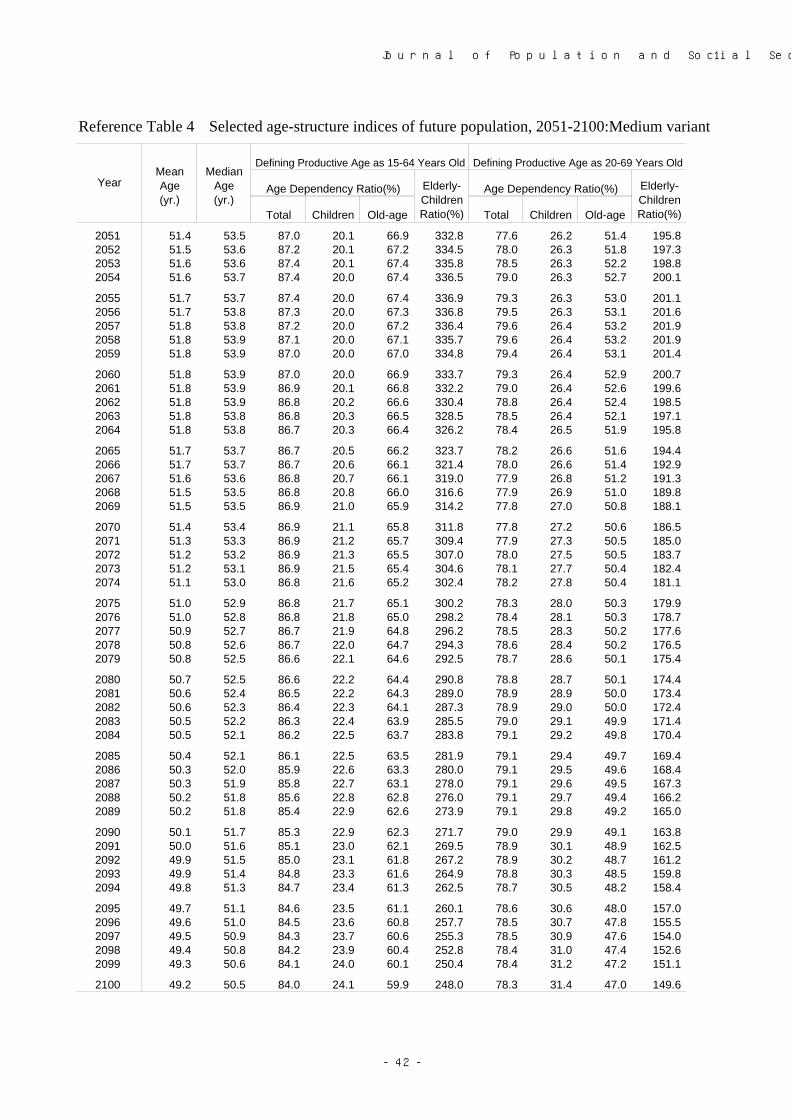
Journal of Population and Social Security (Population) Vol.1 No.1

Reference Table 4 　Selected age-structure indices of future population, 2051-2100:Medium variant

Total Children Old-age Total Children Old-age

2051 51.4 53.5 87.0 20.1 66.9 332.8 77.6 26.2 51.4 195.82052 51.5 53.6 87.2 20.1 67.2 334.5 78.0 26.3 51.8 197.32053 51.6 53.6 87.4 20.1 67.4 335.8 78.5 26.3 52.2 198.82054 51.6 53.7 87.4 20.0 67.4 336.5 79.0 26.3 52.7 200.1

2055 51.7 53.7 87.4 20.0 67.4 336.9 79.3 26.3 53.0 201.12056 51.7 53.8 87.3 20.0 67.3 336.8 79.5 26.3 53.1 201.62057 51.8 53.8 87.2 20.0 67.2 336.4 79.6 26.4 53.2 201.92058 51.8 53.9 87.1 20.0 67.1 335.7 79.6 26.4 53.2 201.92059 51.8 53.9 87.0 20.0 67.0 334.8 79.4 26.4 53.1 201.4

2060 51.8 53.9 87.0 20.0 66.9 333.7 79.3 26.4 52.9 200.72061 51.8 53.9 86.9 20.1 66.8 332.2 79.0 26.4 52.6 199.62062 51.8 53.9 86.8 20.2 66.6 330.4 78.8 26.4 52.4 198.52063 51.8 53.8 86.8 20.3 66.5 328.5 78.5 26.4 52.1 197.12064 51.8 53.8 86.7 20.3 66.4 326.2 78.4 26.5 51.9 195.8

2065 51.7 53.7 86.7 20.5 66.2 323.7 78.2 26.6 51.6 194.42066 51.7 53.7 86.7 20.6 66.1 321.4 78.0 26.6 51.4 192.92067 51.6 53.6 86.8 20.7 66.1 319.0 77.9 26.8 51.2 191.32068 51.5 53.5 86.8 20.8 66.0 316.6 77.9 26.9 51.0 189.82069 51.5 53.5 86.9 21.0 65.9 314.2 77.8 27.0 50.8 188.1

2070 51.4 53.4 86.9 21.1 65.8 311.8 77.8 27.2 50.6 186.52071 51.3 53.3 86.9 21.2 65.7 309.4 77.9 27.3 50.5 185.02072 51.2 53.2 86.9 21.3 65.5 307.0 78.0 27.5 50.5 183.72073 51.2 53.1 86.9 21.5 65.4 304.6 78.1 27.7 50.4 182.42074 51.1 53.0 86.8 21.6 65.2 302.4 78.2 27.8 50.4 181.1

2075 51.0 52.9 86.8 21.7 65.1 300.2 78.3 28.0 50.3 179.92076 51.0 52.8 86.8 21.8 65.0 298.2 78.4 28.1 50.3 178.72077 50.9 52.7 86.7 21.9 64.8 296.2 78.5 28.3 50.2 177.62078 50.8 52.6 86.7 22.0 64.7 294.3 78.6 28.4 50.2 176.52079 50.8 52.5 86.6 22.1 64.6 292.5 78.7 28.6 50.1 175.4

2080 50.7 52.5 86.6 22.2 64.4 290.8 78.8 28.7 50.1 174.42081 50.6 52.4 86.5 22.2 64.3 289.0 78.9 28.9 50.0 173.42082 50.6 52.3 86.4 22.3 64.1 287.3 78.9 29.0 50.0 172.42083 50.5 52.2 86.3 22.4 63.9 285.5 79.0 29.1 49.9 171.42084 50.5 52.1 86.2 22.5 63.7 283.8 79.1 29.2 49.8 170.4

2085 50.4 52.1 86.1 22.5 63.5 281.9 79.1 29.4 49.7 169.42086 50.3 52.0 85.9 22.6 63.3 280.0 79.1 29.5 49.6 168.42087 50.3 51.9 85.8 22.7 63.1 278.0 79.1 29.6 49.5 167.32088 50.2 51.8 85.6 22.8 62.8 276.0 79.1 29.7 49.4 166.22089 50.2 51.8 85.4 22.9 62.6 273.9 79.1 29.8 49.2 165.0

2090 50.1 51.7 85.3 22.9 62.3 271.7 79.0 29.9 49.1 163.82091 50.0 51.6 85.1 23.0 62.1 269.5 78.9 30.1 48.9 162.52092 49.9 51.5 85.0 23.1 61.8 267.2 78.9 30.2 48.7 161.22093 49.9 51.4 84.8 23.3 61.6 264.9 78.8 30.3 48.5 159.82094 49.8 51.3 84.7 23.4 61.3 262.5 78.7 30.5 48.2 158.4

2095 49.7 51.1 84.6 23.5 61.1 260.1 78.6 30.6 48.0 157.02096 49.6 51.0 84.5 23.6 60.8 257.7 78.5 30.7 47.8 155.52097 49.5 50.9 84.3 23.7 60.6 255.3 78.5 30.9 47.6 154.02098 49.4 50.8 84.2 23.9 60.4 252.8 78.4 31.0 47.4 152.62099 49.3 50.6 84.1 24.0 60.1 250.4 78.4 31.2 47.2 151.1

2100 49.2 50.5 84.0 24.1 59.9 248.0 78.3 31.4 47.0 149.6

Defining Productive Age as 20-69 Years Old

Age Dependency Ratio(%) Elderly-ChildrenRatio(%)

YearMeanAge(yr.)

MedianAge(yr.)

Defining Productive Age as 15-64 Years Old

Age Dependency Ratio(%) Elderly-ChildrenRatio(%)

-42-

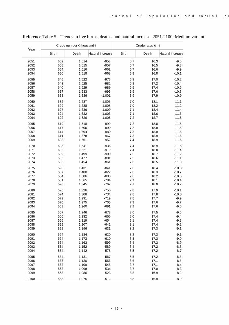
Journal of Population and Social Security (Population) Vol.1 No.1

Reference Table 5 　Trends in live births, deaths, and natural increase, 2051-2100: Medium variant

Birth Death Natural increase Birth Death Natural increase

2051 662 1,614 -953 6.7 16.3 -9.62052 658 1,615 -957 6.7 16.5 -9.82053 654 1,616 -962 6.7 16.6 -9.92054 650 1,618 -968 6.8 16.8 -10.1

2055 646 1,622 -975 6.8 17.0 -10.22056 643 1,625 -982 6.8 17.2 -10.42057 640 1,629 -989 6.9 17.4 -10.62058 637 1,633 -995 6.9 17.6 -10.82059 635 1,636 -1,001 6.9 17.9 -10.9

2060 632 1,637 -1,005 7.0 18.1 -11.12061 629 1,638 -1,008 7.0 18.2 -11.22062 627 1,636 -1,009 7.1 18.4 -11.42063 624 1,632 -1,008 7.1 18.6 -11.52064 622 1,626 -1,005 7.2 18.7 -11.6

2065 619 1,618 -999 7.2 18.8 -11.62066 617 1,606 -990 7.2 18.9 -11.62067 614 1,594 -980 7.3 18.9 -11.62068 611 1,578 -967 7.3 18.9 -11.62069 608 1,561 -952 7.4 18.9 -11.5

2070 605 1,541 -936 7.4 18.9 -11.52071 602 1,521 -919 7.4 18.8 -11.42072 599 1,499 -900 7.5 18.7 -11.22073 596 1,477 -881 7.5 18.6 -11.12074 593 1,454 -861 7.6 18.5 -11.0

2075 590 1,431 -841 7.6 18.4 -10.82076 587 1,408 -822 7.6 18.3 -10.72077 584 1,386 -803 7.6 18.2 -10.52078 581 1,365 -784 7.7 18.1 -10.42079 578 1,345 -767 7.7 18.0 -10.2

2080 576 1,326 -750 7.8 17.9 -10.12081 574 1,308 -734 7.8 17.8 -10.02082 572 1,291 -719 7.8 17.7 -9.92083 570 1,275 -705 7.9 17.6 -9.72084 569 1,260 -691 7.9 17.6 -9.6

2085 567 1,246 -678 8.0 17.5 -9.52086 566 1,232 -666 8.0 17.4 -9.42087 566 1,219 -654 8.1 17.4 -9.32088 565 1,207 -642 8.1 17.4 -9.22089 565 1,196 -631 8.2 17.3 -9.1

2090 564 1,184 -620 8.2 17.3 -9.12091 564 1,173 -610 8.3 17.3 -9.02092 564 1,163 -599 8.4 17.3 -8.92093 564 1,152 -589 8.4 17.2 -8.82094 564 1,142 -578 8.5 17.2 -8.7

2095 564 1,131 -567 8.5 17.2 -8.62096 563 1,120 -556 8.6 17.1 -8.52097 563 1,109 -545 8.7 17.1 -8.42098 563 1,098 -534 8.7 17.0 -8.32099 563 1,086 -523 8.8 16.9 -8.2

2100 563 1,075 -512 8.8 16.9 -8.0

YearCrude number（thousand） Crude rates（‰）

-43-