Population model learned on different stimulus … · Here we introduce a general strategy to equip an arbitrary model of stimulus encoding by single neurons with a network of couplings

Population model learned on different stimulus ensembles predicts network responsesin the retina

Ulisse Ferrari,1, ∗ Stephane Deny,2 Matthew Chalk,1 Gasper Tkacik,3 Olivier Marre,1, 4 and Thierry Mora5, 4

1Sorbonne Universite, INSERM, CNRS, Institut de la Vision, 17 rue Moreau, 75012 Paris, France.2Neural Dynamics and Computation Lab, Stanford University, California

3Institute of Science and Technology, Klosterneuburg, Austria4Equal contribution

5Laboratoire de physique statistique, CNRS, Sorbonne Universite,Universite Paris-Diderot and Ecole normale superieure (PSL), 24, rue Lhomond, 75005 Paris, France

A major challenge in sensory neuroscience is to understand how complex stimuli are collectivelyencoded by neural circuits. In particular, the role of correlations between output neurons is stillunclear. Here we introduce a general strategy to equip an arbitrary model of stimulus encodingby single neurons with a network of couplings between output neurons. We develop a methodfor inferring both the parameters of the encoding model and the couplings between neurons fromsimultaneously recorded retinal ganglion cells. The inference method fits the couplings to accuratelyaccount for noise correlations, without affecting the performance in predicting the mean response.We demonstrate that the inferred couplings are independent of the stimulus used for learning, andcan be used to predict the correlated activity in response to more complex stimuli. The model offersa powerful and precise tool for assessing the impact of noise correlations on the encoding of sensoryinformation.

I. INTRODUCTION

An important goal in sensory neuroscience is to buildmodels that predict how sensory neurons respond to com-plex stimuli—a necessary step towards understanding thecomputations carried out by neural circuits. The collec-tive activity of sensory neurons has been modeled usingdisordered Ising models to account for correlations be-tween cells [1–3]. However this approach cannot predictthe activity of the network in response to a particularstimulus, as it ignores stimulus information. In thesemodels, the correlations captured by the Ising couplingsarise from shared cell dependencies to the stimulus as wellas from shared variability across cells (called noise cor-relations). Ising models have been generalized to includestimulus information through “fields” that modulate thespiking activity and fluctuate as the stimulus changesover time [4, 5], as well as effective couplings betweencells to reflect noise correlations. However, there existsno systematic way to predict how those fields depend onthe stimulus.

In the retina, models have been proposed to predictthe response of single retinal ganglion cells to a given vi-sual stimulation. A common but limited approach is thethe Linear-Non-linear-Poisson (LNP) model [6, 7]. Thismodel is only accurate in restricted cases, e.g. when thestimulus is a full field flicker [8], or has a low spatial res-olution, and is not able to predict the responses of gan-glion cells to stimuli more complex or with fine spatialstructure [9, 10]. Recent studies have used deep con-volutional neural networks to predict the responses ofganglion cells to complex visual scenes [11–13]. These

∗Correspondence should be sent to [email protected].

models have predicted well the responses of single cellsto stimuli with complex spatio-temporal structure [13],and improved significantly the performance in predict-ing the responses to natural scenes [12]. However, thesemodels ignore noise correlations, and it is unclear if theycan predict the joint activity of a population of ganglioncells. Ganglion cells are not deterministic, and show in-trinsic variability in the response, even when presentedwith identical repetitions of the same stimulus. Someof this variability is correlated between different cells, aswas shown for neighboring cells of the same type [14–17].A possible explanation for this correlated noise is thatganglion cells of the same type are connected to eachother through gap junctions, at least in the rodent retina[18]. These direct connections between ganglion cells arenot taken into account by convolutional models, whichtreat each cell independently.

Here we build a model that combines a feed-forwardmulti-layer network to process the stimulus [13], and aninteraction network of couplings between output neuronsto account for noise correlations. We develop a strategyto learn this model on physiological data and to fit thecouplings to reproduce solely noise correlations. We val-idate the approach by showing that couplings learned onone stimulus ensemble can successfully predict the corre-lated activity of the population in response to a very dif-ferent stimulus. Thus, inferred couplings are independentof the stimulus used to learn them, and can be used topredict the correlated activity in response to more com-plex stimuli. This strategy is not restricted to the specificstimulus-processing model considered here in the contextof retinal ganglion cells, and can be applied to generalizeany model predicting the mean spiking activity of singlecells.

not peer-reviewed) is the author/funder. All rights reserved. No reuse allowed without permission. The copyright holder for this preprint (which was. http://dx.doi.org/10.1101/243816doi: bioRxiv preprint first posted online Jan. 5, 2018;

http://dx.doi.org/10.1101/243816

2

II. NOISE CORRELATIONS IN CELLS OF THESAME TYPE

We re-analyzed [13] a dataset of ex-vivo recording ofthe activity of retina ganglion cells (RGCs) in Long-Evans adult rats using a multi-electrode array (seeFig. 1A top for an example response). The stimulus wasa movie of two parallel bars, whose trajectories followedthe statistics of two independent overdamped stochasticoscillators. Additionally a random binary checkerboardand a sequence of specifically devoted stimuli were pro-jected for one hour to allow for receptive field estimationand RGC type identification. Raw voltage traces werestored and spike-sorted off-line through a custom spikesorting algorithm [19].

We applied a standard clustering analysis based on thecell response to various stimuli to isolate a population ofOFF ganglion cells of the same type. Their receptivefields tiled the visual field to form a mosaic (Fig. 1B).

The ganglion cell spike times were binned at ∼ 17ms(locked to the stimulus frame rate) to estimate the em-pirical spike counts, ni(t) ∈ [0, 1, 2, . . . ] for cell i dur-ing time-bin t (see Fig. 1A bottom). The stimulus al-ternates between non-repeated sequences of random bartrajectories, and a repeated sequence of randomly mov-ing bars, displayed 54 times. Non-repeated sequenceswere divided into training (two thirds of the total) andtesting (one third) sets. Repeated sequences were equallydivided into training and testing sets by splitting the re-peated trajectory in two different halves. We estimatethe Peri-Stimulus Time Histogram (PSTH), i.e. averagefiring rate over time in response to the repeated stimu-lus sequence, as λi(t) ≡ 〈ni(t)〉repeat for cell i, (Fig. 1A

bottom) and its average, λi ≡ (1/T )∑Tt=1 λi(t).

We measured the correlated variability between pairs

of cells (example in Fig. 1C) computed from the repeateddataset between two cells. The total pairwise covarianceis the sum of stimulus (c(S)) and noise (c(N)) covariances.The first can be computed as the cross-covariance of thePSTH (black line), which estimates the correlation be-tween cells induced by the stimulus:

c(S)ij (t− t′) ≡ 1

T

T∑t=1

(λi(t)− λi)(λj(t′)− λj) (1)

The difference between the total cross-covariance and thestimulus covariance is the noise covariance:

c(N)ij (t− t′) ≡ 1

T

T∑t=1

〈(ni(t)− λi(t))(nj(t′)− λj(t′))〉repeat

(2)Noise covariances are significantly different from zeroonly at zero lag (t = t′), meaning that they happen at ashort time scale, which suggests they may be due to gap-junctions [14, 20]. Only cells that were physically closehad large noise correlations (Fig. 1D), and their valuesstrongly decreased with distance.

III. INDEPENDENT CELL MODEL

We aim at developing a population model of the RGCresponse to visual stimuli. First we develop a feed-forward model to predict how each cell responds indi-vidually to the stimulus. Second, we will add recurrentinteractions to the model to account for noise correla-tions. We build LN2E , a model composed of a cascadeof two layers of Linear-Non-linear units. This model aims

at predicting the cell firing rate λi(t) as a function λi[St]of the stimulus S. Spikes are then generated as drawsfrom the Effective (E) model described in [21]:

PLN2E

(ni(t)

∣∣St ) = exp{hi[St]ni(t)− γ ni(t)2 − δ ni(t)3 − log ni(t)!− logZt

}(3)

hi[St] such that 〈ni(t)〉PLN2E= λi[St] . (4)

where Zt = Z[St, γ, δ] is the partition function. γ andδ are parameters of a simple model that allows effi-cient modeling of the sub-Poisson variability, and accu-

rately reproduce the spike count variance [21]. hi[St] isa uniquely defined function of γ and δ that constraints

the average of n(t) to equal λi[St], much like in classicalphysics a chemical potential can be tuned to impose themean number of particle in the system.

A. LN2E model

Within the LN2E model [13, 21], the stimulus S(x, t),representing the time behavior of each pixel, is first con-volved with a Gaussian and biphasic factorized kernelKBP(x, t) and then passed through Rectified QuadraticUnits with the two possible polarities:

Θ[St] = Θ(x, t) ≡[

Θ(x, t)ON , Θ(x, t)OFF]

(5)

=[

NLON(KBP ? S

), NLOFF

(KBP ? S

) ](6)

where ? means spatial and temporal convolution andNLON and NLOFF correspond to rectified square


http://dx.doi.org/10.1101/243816

3

A B C D

0 1 2 3 40

60

-100 0 100

0

0.02

0.04

0.06

0.08DataRate

0 0.2 0.4 0.6 0.80

0.01

0.02

0.03

0.04

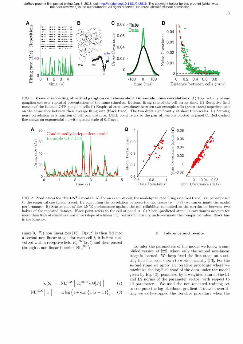
FIG. 1: Ex-vivo recording of retinal ganglion cell shows short time-scale noise correlations. A) Top: activity of oneganglion cell over repeated presentations of the same stimulus. Bottom: firing rate of the cell across time. B) Receptive fieldmosaic of the isolated OFF ganglion cells C) Empirical cross-covariance between two example cells (green trace) superimposedon the covariance between their average firing rate (black trace). The two differ significantly at short time-scales. D) Zero-lagnoise correlation as a function of cell pair distance. Black point refers to the pair of neurons plotted in panel C. Red dashedline shows an exponential fit with spatial scale of 0.11mm.

A B C

0 1 2 3 4 50

20

40

60

80

0.6 0.8 10.6

0.7

0.8

0.9

1

0 0.04 0.08

-0.02

0

0.02

0.04

0.06

0.08

FIG. 2: Prediction for the LN2E model. A) For an example cell, the model-predicted firing rate (red trace) is super-imposedto the empirical one (green trace). By computing the correlation between the two traces (ρ = 0.87) we can estimate the modelperformance. B) Scatter-plot of the LN2E performance against the cell reliability, computed as the correlation between twohalves of the repeated dataset. Black point refers to the cell of panel A. C) Model-predicted stimulus covariances account formore than 84% of stimulus covariance (slope of a linear fit), but systematically under-estimate their empirical value. Black lineis the identity.

(max(0, · 2)) non linearities [13]. Θ(x, t) is then fed intoa second non-linear stage: for each cell i, it is first con-volved with a receptive field KRGC

i (x, t) and then passed

through a non-linear function NLRGCi :

λi[St] = NLRGCi

[KRGCi ?Θ[St]

](7)

NLRGCi

[x]

= ai log(

1 + exp{bi(x+ ci)

}). (8)

B. Inference and results

To infer the parameters of the model we follow a sim-plified version of [22], where only the second non-linearstage is learned. We keep fixed the first stage on a set-ting that has been shown to work efficiently [13]. For thesecond stage we apply an iterative procedure where wemaximize the log-likelihood of the data under the modelgiven by Eq. (3), penalized by a weighted sum of the L1and L2 norms of the parameter vector, with respect toall parameters. We used the non-repeated training setto compute the log-likelihood gradient. To avoid overfit-ting we early-stopped the iterative procedure when the


http://dx.doi.org/10.1101/243816

4

log-likelihood computed on the non-repeated testing setstopped to increase. L1 and L2 penalties were optimizedby maximizing the performance on the repeated datasetthat later we will use for training the population model.

In Fig. 2A we compare the time course of the em-pirical firing rate, λi(t), with the prediction of the in-ferred LN2E model for an example cell. By comput-ing the Pearson correlation among these two temporaltraces (ρ = 0.87), we can estimate the performance ofthe model for each cell. In Fig. 2B we compare this per-formance with the reliability of the retinal spike activity,estimated as the correlation between two disjoint subsetsof responses to the repeated stimulus and found that theywere comparable. In Fig. 2C we show how the model pre-

dicts the empirical stimulus covariances. Even if a smallunder-estimation is present, the model accounts for morethan the 84% of the empirical value (slope of a linear fit).

IV. POPULATION MODEL

We then build a population model that accounts fornoise correlation, starting from the LN2E . From themodel in the form Eq. (3) we build a two layers Linear-Non-linear Population Effective model, LN2PE , byadding a pairwise interaction term:

PLN2PE

(n(t)

∣∣S,J )= exp

{∑i

(hi[St]ni(t)− γ ni(t)2 − δ ni(t)3− log ni(t)!

)+∑i≤j

Jijni(t)nj(t)− logZt

}(9)

hi[St] such that 〈ni(t)〉PLN2PE

= λi[St] . (10)

where Zt ≡ Z[St, γ, δ,J

]is the normalization constant.

The terms Jii are assumed to be independent of i, andare a correction to γ due to the impact of the population.The model is thus designed such that the conditionalprobability distribution of any spike count ni(t) reducesto an Effective model (Eq. (3)), when the activity of allthe others neurons is fixed.

A. Inference of the interaction network

One possibility to infer the LN2PE model could havebeen to estimate the couplings by maximizing likelihoodon the non-repeated dataset, similar to [4]. However,the issue with this approach is that it does not distin-guish between signal and noise correlation. As a result, ifthe feed-forward model does not reproduce perfectly thesignal correlation, the interaction parameters will try tocompensate this error. We observed this effect by infer-ring a Generalized Linear Model (GLM) [7], see App. A.

Straightforward likelihood maximization cannot guaran-tee that coupling terms only reflect noise correlations;rather, they reflect an uncontrolled combination or mix-ture of signal and noise correlations, which have verydifferent biological interpretations. An extreme versionof this phenomenon can be found in [4], Fig. 15, wherethe response of one neuron to a natural scene is predictedfrom the responses of other neurons, without any use ofthe stimulus. In our case we want to have couplings re-flecting solely noise correlations. We therefore developedan alternative inference method.

In order to obtain the parameters values J that ac-count solely for noise correlations, we need a model thatreproduces perfectly the time course of the firing rate.To construct such a model we use repetitions of the samestimulation, to estimate the empirical rate and imposeit with Lagrange multipliers. To this aim we recast theLN2PE model in a Time Dependent Population Effective(TDPE) model [4]:

PTDPE

(n(t)

∣∣J,h ) ∼ exp

∑i

(hi(t)ni(t)− γ ni(t)2 − δ ni(t)3 − log ni(t)!

)+∑i≤j

Jijni(t)nj(t)

(11)

where we have substituted the stimulus dependent input-

rate hi[St] with Lagrange multipliers hi(t) enforcing theempirical mean spike count, 〈ni(t)〉 = λi(t), for each cell

in each time-bin of the repeated stimulation. TDPE isnot a real stimulus model, as it can not predict the spik-ing activity in response to stimuli different from the one


http://dx.doi.org/10.1101/243816

5

A B C

0 0.5 1

0

0.2

0.4

0.6

0.8

1

0 0.02 0.04-0.01

0

0.01

0.02

0.03

0.04

0.05

0 0.2 0.4 0.6 0.8

0

0.5

1

1.5

FIG. 3: Time-dependent inference provides good estimates of the interaction network. A) Comparison betweenthe inferred interaction from first (later used as training) and second (later used as testing) halves of the repeated dataset.Black line is the identity. B) Comparison of the predicted noise correlations when the interaction matrix J learned using thetraining set is applied to the testing set. Black line is the identity. C) The behavior with distance of the inferred interactionsscales similarly to that of noise correlations (see Fig. 1D), although it goes to zero at shorter distances. Red dashed line is anexponential fit with spatial constant 0.08mm.

used for training. However the learned J will accountsolely for noise correlations as stimulus correlations arereproduced by construction.

We will proceed as follows: At first we will learn Jand h of the model (11) on repeated sequences of thestimulus. As the model (11) belongs to the exponentialfamily, the inference can be easily performed by maxi-mizing the log-likelihood (see for example [23]). We adda small L2 penalty (with coefficient η L2 ∼ 2 · 10−6)over the biases h simply to avoid divergences to −∞when 〈ni(t)〉repeat = 0. In order to avoid spurious non-zero values, we also add a L1 penalty (with coefficentη L1 = 0.04). Fig. 3 shows the results of the TDPE in-ference. In order to evaluate the robustness of the in-ference with respect to a change of dataset, in Fig. 3Awe plot the interactions inferred from the training setagainst those inferred from another training set of thesame size. The comparison shows that inferred networksare robust against a change of stimulus.

We will use the values found for the parameters Jijwhen inferring the model (11) in the first step, and keepthese parameters fixed during the second step of the in-ference, where we will learn the rest of the parameters ofthe population model (Eq. (9)).

To check the validity of this approach, in Fig. 3B wefirst compare empirical noise correlations obtained withthe test dataset with those predicted by the model. Toobtain this prediction, we freeze the J value obtainedfrom the inference on the training set and we re-infer thehi(t) to match the firing rates of the testing set. Theinferred parameters J were able to predict well the noisecorrelation on a part of the recording that had not beenused to learn them. In panel C we show the behavior ofthe interaction parameters as a function of the distancebetween the corresponding cell couple. J decreases with

distance slightly faster than noise correlation, see Fig. 1.The good quality of the inference allows us now to

apply the inferred interaction network on top of the singlecell model.

B. Complete model inference

Now that we have inferred the network J we can buildthe LN2PE model, presented in Eq. (9). The last stepto perform is to adjust the parameters that specify thefields as a function the stimulus h[St]

Because of the interaction term, each cell receives arandom input

∑j Jijnj(t) from the rest of the network.

This random contribution is responsible for the noise cor-relation. However it generates also a mean contribution

∆hi[St] that may affect the cell firing rate and if not re-moved, will impact the firing rate prediction. Because ofnetwork effects, this mean contribution differs from its

mean value: ∆hi[St] 6=∑i 6=j Jij λj(t). In order to esti-

mate it, we compute the Thouless, Anderson and Palmer(TAP) free energy formalism of the model (9) [24] and use

it to derive an approximation for ∆hi[St]. We followedstrictly [25] and [26] and apply a second order Plefka ex-pansion [27] (see App.B for more details). The resultis:

∆hi[St] ≈∑j 6=i

Jij λj [St] + Jii

(V ′(λi[St]

)+ 2λi[St]

)+

1

2V ′(λi[St]

)∑j 6=i

J2ijV(λj [St]

)+

1

2J2iiW

′(λi[St])

(12)

where the first two terms are the mean-field contributions


http://dx.doi.org/10.1101/243816

6

of network and self couplings, whereas the lasts two aretheir Onsager [28] reaction terms. Together with theirderivatives, in (12) we have introduced

V (λ) ≡ P(2)λ − P (1)

λ P(1)λ (13)

W (λ) ≡ P(4)λ − P (2)

λ P(2)λ −

(P

(3)λ − P (2)

λ P(1)λ

)2V (λ)

(14)

where P(s)λ ≡ 〈ns〉E are the moments of n computed

within an Effective model with the same structure asEq. (3), but with parameter hi tuned to enforce the meanspike count, 〈n〉E = λ. Note that the correction (12) isa stimulus dependent quantity because it depends onlyon inputs λ[St] and not on the spike counts n(t). Con-sequently it can be reabsorbed within the form (9) bysubstituting:

hPEi [St] = hEi [St]−∆hi[St] (15)

hEi [St] such that 〈ni(t)〉PLN2E

= λi[St] , (16)

where 〈ni(t)〉PLN2E

is computed with the conditionally

independent model LN2E , not the population model asin (9). Computing this correction requires only somematrix multiplications and can thus be evaluated easilyfor a new stimulus.

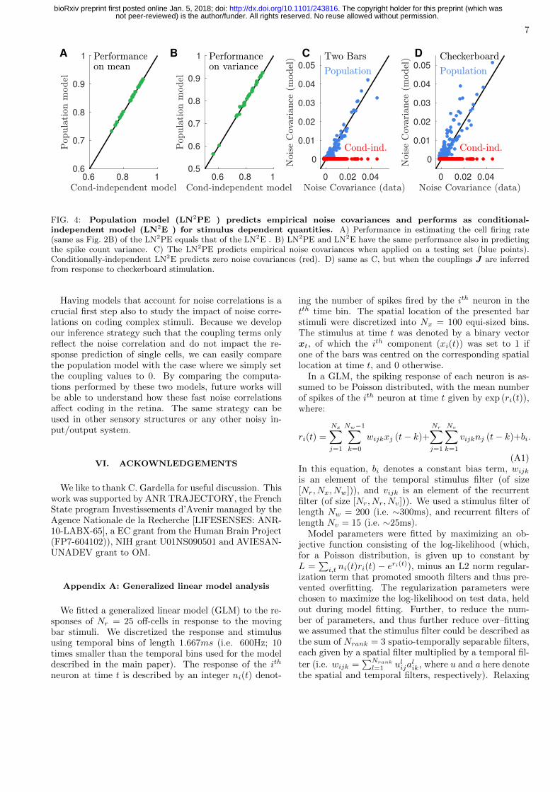
In Fig. 4A and B, we check that the inferring the pop-ulation model still preserves the quality of the predic-tion of single cell activity obtained with the independentmodel. We compare the performance of the two modelsin reproducing the firing rate of the recorded cells (samequantity as Fig. 2B). Firing rate is a stimulus dependentquantity and accordingly the two models have similarperformance. The fact that LN2PE has not smaller per-formance than LN2E ensures the quality of the estima-tion of the corrections ∆h[St] with the TAP approach.Whereas the fact that it is neither larger ensures that thecouplings do not help the model in predicting stimulus-dependent, average quantities but can account only fornoise fluctuations. Panel B shows that thanks to the selfinteraction term, LN2E and LN2PE have similar perfor-mance also for spike count variance.

Fig. 4C shows how the LN2PE model outperforms theLN2E in predicting the population activity. The coupledLN2PE model accounts well for noise covariances on atesting set (blue points). Because it is an independentcell model, the LN2E predicts vanishing noise covariance(red points).

C. Generalizing to other types of stimuli

A major challenge with fitting complex encoding mod-els to neural responses is that they rarely generalize well.Here we ask if the interaction network can be inferredfrom a qualitatively different stimulus and then appliedto our two-bars stimulation. To test for this, we inferthe couplings as in the section IV A, but on the response

to repeated checkerboard stimuli. We then use this newset of couplings to equip the conditionally-independentLN2E we have previously inferred on the moving barstimulus and obtain a new LN2PE model. In panel D weshow that this LN2PE model predicts noise covarianceswhen applied to the two-bars testing set. This shows thatour inference method allows to generalize from one stim-ulus type to the other, because the couplings betweencells seem invariant to the stimulus here.

V. DISCUSSION

We have shown a method to infer a model from popula-tion recordings, which takes into account both the impactof the stimulus, through a feed-forward network, and thecorrelated noise between cells, thanks to a coupling net-work. Note that the interactions between cells are heredescribed as “instantaneous”. The activity of one cell attime t will affect other cells at time bin t, not t+ 1. Thisis due to the fact that the noise correlations between cellsare very fast. We chose a time bin of the magnitude ofthe time constant of these correlations.

Previous approaches [4, 7] have aimed at reproducingnoise correlations, but the stimulus could only influencethe response through a linear filter. When reduced to asingle cell, these models were similar to the classical LNmodel. Conversely, non-linear models derived from con-volutional networks [12, 13] did not try to model noisecorrelations. Here we take the best of both approaches,and developed a method to infer both the parameters de-scribing the influence of the stimulus, and the couplingvalues. Our method is general and could be applied toother structures than the retina. Furthermore, it can bestraightforwardly extended to models where the influenceof the stimulus on single cell activity is described by dif-ferent non-linear models, e.g. a deep network with morelayers [12].

We have developed an inference strategy that allowsthe coupling term to reflect solely shared noise acrossneurons, without the interference of stimulus effects dueto artifacts of the learning procedure. Such effects canarise when the inference procedure tries to use the ac-tivity of other cells as a surrogate of the stimulus itselfto improve the predictability of a given cell, compensat-ing for non-linearities in the stimulus dependence thatare unaccounted by the model. Consequently, couplingsshow a weak dependence on the actual stimulus ensembleused to learn them. This allowed us to to show that theirvalue can be inferred even from a qualitatively differentstimulus. Note that checkerboard and two-bars stimu-lations drive very different responses of the retina. It isthus a remarkable result that noise correlations in theresponse to a complex video of moving objects can bepredicted by couplings inferred from responses to stim-uli. This result can thus be seen as a first step towardthe construction of a full model that accounts for largeand heterogeneous stimulus ensembles.


http://dx.doi.org/10.1101/243816

7

A B C D

0.6 0.8 10.6

0.7

0.8

0.9

1

0.6 0.8 10.5

0.6

0.7

0.8

0.9

1

0 0.02 0.04

0

0.01

0.02

0.03

0.04

0.05

0 0.02 0.04

0

0.01

0.02

0.03

0.04

0.05

FIG. 4: Population model (LN2PE ) predicts empirical noise covariances and performs as conditional-independent model (LN2E ) for stimulus dependent quantities. A) Performance in estimating the cell firing rate(same as Fig. 2B) of the LN2PE equals that of the LN2E . B) LN2PE and LN2E have the same performance also in predictingthe spike count variance. C) The LN2PE predicts empirical noise covariances when applied on a testing set (blue points).Conditionally-independent LN2E predicts zero noise covariances (red). D) same as C, but when the couplings J are inferredfrom response to checkerboard stimulation.

Having models that account for noise correlations is acrucial first step also to study the impact of noise corre-lations on coding complex stimuli. Because we developour inference strategy such that the coupling terms onlyreflect the noise correlation and do not impact the re-sponse prediction of single cells, we can easily comparethe population model with the case where we simply setthe coupling values to 0. By comparing the computa-tions performed by these two models, future works willbe able to understand how these fast noise correlationsaffect coding in the retina. The same strategy can beused in other sensory structures or any other noisy in-put/output system.

VI. ACKOWNLEDGEMENTS

We like to thank C. Gardella for useful discussion. Thiswork was supported by ANR TRAJECTORY, the FrenchState program Investissements d’Avenir managed by theAgence Nationale de la Recherche [LIFESENSES: ANR-10-LABX-65], a EC grant from the Human Brain Project(FP7-604102)), NIH grant U01NS090501 and AVIESAN-UNADEV grant to OM.

Appendix A: Generalized linear model analysis

We fitted a generalized linear model (GLM) to the re-sponses of Nr = 25 off-cells in response to the movingbar stimuli. We discretized the response and stimulususing temporal bins of length 1.667ms (i.e. 600Hz; 10times smaller than the temporal bins used for the modeldescribed in the main paper). The response of the ith

neuron at time t is described by an integer ni(t) denot-

ing the number of spikes fired by the ith neuron in thetth time bin. The spatial location of the presented barstimuli were discretized into Nx = 100 equi-sized bins.The stimulus at time t was denoted by a binary vectorxt, of which the ith component (xi(t)) was set to 1 ifone of the bars was centred on the corresponding spatiallocation at time t, and 0 otherwise.

In a GLM, the spiking response of each neuron is as-sumed to be Poisson distributed, with the mean numberof spikes of the ith neuron at time t given by exp (ri(t)),where:

ri(t) =

Nx∑j=1

Nw−1∑k=0

wijkxj (t− k)+

Nr∑j=1

Nv∑k=1

vijknj (t− k)+bi.

(A1)In this equation, bi denotes a constant bias term, wijkis an element of the temporal stimulus filter (of size[Nr, Nx, Nw])), and vijk is an element of the recurrentfilter (of size [Nr, Nr, Nv])). We used a stimulus filter oflength Nw = 200 (i.e. ∼300ms), and recurrent filters oflength Nv = 15 (i.e. ∼25ms).

Model parameters were fitted by maximizing an ob-jective function consisting of the log-likelihood (which,for a Poisson distribution, is given up to constant byL =

∑i,t ni(t)ri(t) − eri(t)), minus an L2 norm regular-

ization term that promoted smooth filters and thus pre-vented overfitting. The regularization parameters werechosen to maximize the log-likelihood on test data, heldout during model fitting. Further, to reduce the num-ber of parameters, and thus further reduce over–fittingwe assumed that the stimulus filter could be described asthe sum of Nrank = 3 spatio-temporally separable filters,each given by a spatial filter multiplied by a temporal fil-

ter (i.e. wijk =∑Nrank

l=1 ulijalik, where u and a here denote

the spatial and temporal filters, respectively). Relaxing


http://dx.doi.org/10.1101/243816

8

this assumption (by increasing Nrank) did not improvethe quality of the model fit.

We fitted two versions of the GLM model to therecorded neural responses: first, a ‘coupled model’ withfiring rate described by equation A1; second, an uncou-pled model, in which the recurrent filters, v, were set tozero. Figure 5 plots the firing rate of a single recordedOFF-cell (also plotted in Fig. 2A of the main text), along-side the predictions by the coupled and uncoupled GLMmodels. The coupled model gave a different prediction forthe cell’s firing rate, compared to the uncoupled model.Further, plotting the Pearson correlation between empir-ical firing rate and the predictions by both model variantsfor each cell (Figure 5b), shows that the coupled modelgives an improved prediction of the recorded PSTH fornearly all recorded OFF-cells, compared to the uncou-pled model. Thus, in addition to fitting the interactionsbetween different neurons (i.e. the noise correlations), the

coupled GLM model used the recurrent filters, v, to im-prove the prediction of how each neuron responded to thestimulus (i.e. the stimulus correlation).

Appendix B: Construction of the mean-field theoryand Thouless-Anderson-Palmer correction

We are interested in computing the TAP correctionto the fields hi(t) due to the addition of the couplingterm J to the conditionally-independent LN2E model (3).Because we are not interested in the TAP expression forcouplings nor in that for covariances, we can constructthe mean-field theory for a single time-bin. Otherwise,because the couplings are constant in time we shouldhad considered the whole model. To apply the Plefkaexpansion we introduce:

F [α,h, J ] ≡ − log∑n

exp

N∑i=1

(hini − γ n2 − δ n3 − log n!

)+ α

∑i<j

Jijninj

(B1)

and its Legendre transform:

G[α,λ, J ] =

(∑i

hiλi + F [α,h, J ]

∣∣∣∣∣h=h

(B2)

where h = h[α,λ] is defined implicitly from:

∂(∑

i hiλi + F [α,h, J ])

∂hi

∣∣∣∣∣∣h=h

= λi − 〈ni〉(α)∣∣∣h=h

= 0

(B3)where 〈. . . 〉(α) is the average with respect to the distri-bution related to the free energy (B1). Our goal is toexpand G(α,λ, j) around α = 0 up to the second order.At first we evaluate the derivatives:

G′[α,λ, J ] = −∑i<j

Jij〈ninj〉(α) (B4)

G′′[α,λ, J ] = −∑i<j

∑k≤l

JijJkl〈ninjnknl〉(α)c

+∑i<j

Jij∑g

∂hg∂α〈ninj(ng − λg)〉(α) (B5)

∂hg∂α

=

⟨∑k≤l Jklnknl(ng − λg)

⟩(α)〈n2g〉

(α)c

(B6)

where to obtain the last equality we applied the implicitfunction theorem to Eq. (B3). To compute the term of

the Plefka expansion we need to evaluate G[α,λ, J ] and

its derivatives at α = 0. To this aim we note that hi[α =

0,λ] = hi[λi], as for α = 0 the system units become

independent and consequently hi depends only on λi. Forα = 0, in fact, the distribution over {ni}Ni=1 factorizesover a set of single variable distributions. this allowsus to compute model expectations at α = 0. For futureconvenience, we define the moments of such distributions:

P (s) ≡ 〈ns〉(α=0) (B7)

so that the terms in the expansion become:

G[0,λ, J ] =∑i

hiλi + F [α = 0, h] (B8)

G′[0,λ, J ] = −∑i<j

Jijλiλj −∑i

JiiP(2)i (B9)

G′′[0,λ, J ] = −∑i<j

J2ij

(P

(2)i − λ2i

)(P

(2)j − λ2j

)−∑i

J2iiWi (B10)

where W has been defined in Eq. (14). We can nowobtain an approximation for G[λ, J ] = G[α = 1,λ, Jdefined in Eq. (B2) as:

G[λ, J ] ≈ G[0,λ, J ] + α G′[0,λ, J ] (B11)

+1

2α2 G′′[0,λ, J ] +O(α3) (B12)


http://dx.doi.org/10.1101/243816

9

0 1 2 3 4 50

20

40

60

80

0.4 0.5 0.6 0.7 0.8 0.9 10.6

0.7

0.8

0.9

1

time (s) uncoupled model

coup

led

mod

el 1

0.9

0.8

0.7

0.60.4 0.6 0.8 1.0

60

40

20

0

firin

g ra

te (H

z)

0 1 2 3 4 5

A BExample OFF-cell Coupled GLM Uncoupled GLM

FIG. 5: Effect of adding recurrent filters in a generalised-linear-model (GLM) fit to the recorded neural responses. (A) Examplefiring rate of a single cell (green), alongside the predictions of the coupled (blue) and uncoupled (red) GLM fits. (B) Correlationcoefficient between the firing rate predicted by the coupled (y-axis) and uncoupled (x-axis) GLM models and the data, for eachcell. The cell shown in panel A is shown in black.

The mean-field equation for the fields h can be easilyobtained by a reverse Legendre transform:

hi =∂G[λ, J ]

∂λi(B13)

= hi[λi] +∂G′[0,λ, J ]

∂λi+

1

2

∂G′′[0,λ, J ]

∂λi(B14)

which provides the expression (12) for the TAP correc-tion.

[1] Schneidman E, Bialek W, Berry MJ (2003) Synergy, re-dundancy, and independence in population codes. Jour-nal of Neuroscience 23:11539–11553.

[2] Schneidman E, Berry M, Segev R, Bialek W (2006) Weakpairwise correlations imply strongly correlated networkstates in a population . Nature 440:1007.

[3] Tkacik G, et al. (2014) Searching for collective behaviourin a network of real neurons . PloS Comput. Biol.10(1):e1003408.

[4] Granot-Atedgi E, Tkacik G, Segev R, Schneidman E(2013) Stimulus-dependent maximum entropy models ofneural population codes. PLOS Computational Biology9:1–14.

[5] Tkacik G, Granot-Atedgi E, Segev R, Schneidman E(2013) Retinal metric: A stimulus distance measure de-rived from population neural responses. Phys. Rev. Lett.110:058104.

[6] Chichilnisky E (2001) A simple white noise analysis ofneuronal light responses. Network: Computation in Neu-ral Systems 12:199–213.

[7] Pillow J, et al. (2008) Spatio-temporal correlations andvisual signalling in a complete neuronal population. Na-ture 454:995–999.

[8] Berry II MJ, Meister M (1998) Refractoriness and neuralprecision pp 110–116.

[9] Gollisch T, Meister M (2010) Eye smarter than scientistsbelieved: Neural computations in circuits of the retina.Neuron 65:150–64.

[10] Heitman A, et al. (2016) Testing pseudo-linear models ofresponses to natural scenes in primate retina. bioRxiv.

[11] Vintch B, Movshon JA, Simoncelli EP (2015) A convolu-

tional subunit model for neuronal responses in macaquev1. Journal of Neuroscience 35:14829–14841.

[12] McIntosh L, Maheswaranathan N, Nayebi A, Ganguli S,Baccus S (2016) Deep learning models of the retinal re-sponse to natural scenes pp 1361–1369.

[13] Deny S, et al. (2017) Multiplexed computations in retinalganglion cells of a single type. Nature communications8:1964.

[14] Brivanlou I, Warland D, Meister M (1998) Mechanisms ofConcerted Firing among Retinal Ganglion Cells. Neuron20:527–539.

[15] Shlens J, Rieke F, Chichilnisky E (2008) Synchronizedfiring in the retina. Current opinion in neurobiology18:396–402.

[16] Greschner M, et al. (2011) Correlated firing among majorganglion cell types in primate retina. The Journal ofPhysiology 589:75–86.

[17] Ala-Laurila P, Greschner M, Chichilnisky E, Rieke F(2011) Cone photoreceptor contributions to noise andcorrelations in the retinal output. Nature neuroscience14:1309–1316.

[18] Volgyi B, Chheda S, Bloomfield S (2009) Tracer couplingpatterns of the ganglion cell subtypes in the mouse retina.J. Comp. Neurol. 512:664–687.

[19] Yger P, et al. (2016) Fast and accurate spike sortingin vitro and in vivo for up to thousands of electrodes.bioRxiv.

[20] Trenholm S, et al. (2014) Nonlinear dendritic integrationof electrical and chemical synaptic inputs drives fine-scalecorrelations. Nature neuroscience 17:1759–1766.

[21] Ferrari U, Deny S, Marre O, Mora T (2018) A sim-


http://dx.doi.org/10.1101/243816

10

ple model for low variability in neural spike trains.bioRxiv/2018/243543.

[22] McFarland JM, Cui Y, Butts DA (2013) Inferring nonlin-ear neuronal computation based on physiologically plau-sible inputs. PLoS Comput Biol 9:e1003143.

[23] Ferrari U (2016) Learning maximum entropy modelsfrom finite-size data sets: A fast data-driven algorithmallows sampling from the posterior distribution. Phys.Rev. E 94:023301.

[24] Thouless D, Anderson P, Palmer R (1977) Solvable modelof a spin glass. Phil. Mag. 35:593.

[25] Kappen H, Rodriguez F (1997) Efficient learning in boltz-mann machines using linear response theory.. NeuralComput. 10:1137–1156.

[26] Tanaka T (1998) Mean-field theory of Boltzmann ma-chine learning. Phys. Rev. E 58:2302.

[27] Plefka T (1982) Convergence condition of the tap equa-tion for the infinite-ranged ising spin glass model. Journalof Physics A: Mathematical and general 15:1971.

[28] Onsager L (1936) Electric moments of molecules in liq-uids. Journal of the American Chemical Society 58:1486–1493.


http://dx.doi.org/10.1101/243816

Documents

Population model learned on different stimulus … · Here we introduce a general strategy to equip an arbitrary model of stimulus encoding by single neurons with a network of couplings