A Model of the Consumption Response to Fiscal

Stimulus Payments*

Greg Kaplan

University of Pennsylvania and IFSgkaplan@sas.upenn.edu

Giovanni L. Violante

New York University, CEPR, and NBERglv2@nyu.edu

this draft: August 2011

Abstract

A wide body of empirical evidence, based on randomized experiments, finds that 20-40 percent of fiscal

stimulus payments (e.g. tax rebates) are spent on nondurable household consumption in the quarter

that they are received. We develop a structural economic model to interpret this evidence. Our model

integrates the classical Baumol-Tobin model of money demand into the workhorse incomplete-markets

life-cycle economy. In this framework, households can hold two assets: a low-return liquid asset (e.g.,

cash, checking account) and a high-return illiquid asset (e.g., housing, retirement account) that carries

a transaction cost. The optimal life-cycle pattern of wealth accumulation implies that many households

are “wealthy hand-to-mouth”: they hold little or no liquid wealth despite owning sizeable quantities

of illiquid assets. They therefore display large propensities to consume out of additional income. We

document the existence of such households in data from the Survey of Consumer Finances. A version

of the model parameterized to the 2001 tax rebate episode is able to generate consumption responses

to fiscal stimulus payments that are in line with the data.

Keywords: Consumption, Fiscal Stimulus Payments, Hand-to-Mouth, Liquidity.

JEL Classification: D31, D91, E21, H31

*We thank Kurt Mitman for outstanding research assistance, and Jonathan Heathcote for his insightfulcomments at the early stage of this research.

1 Introduction

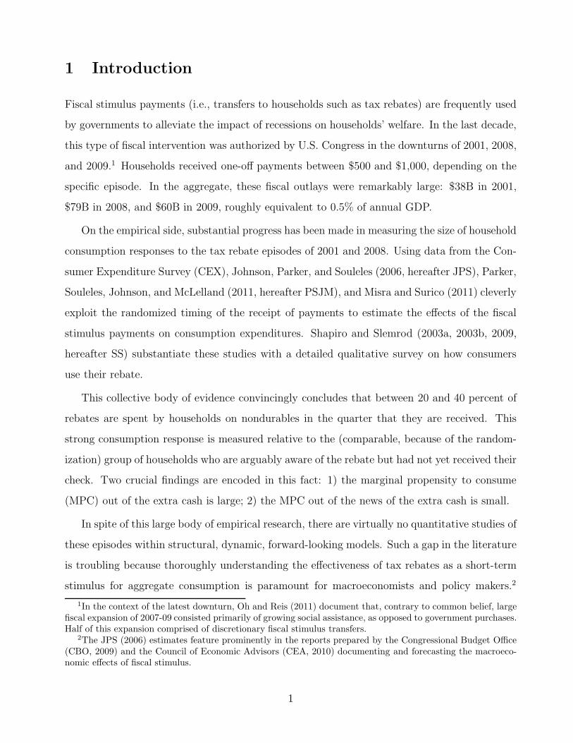
Fiscal stimulus payments (i.e., transfers to households such as tax rebates) are frequently used

by governments to alleviate the impact of recessions on households’ welfare. In the last decade,

this type of fiscal intervention was authorized by U.S. Congress in the downturns of 2001, 2008,

and 2009.1 Households received one-off payments between $500 and $1,000, depending on the

specific episode. In the aggregate, these fiscal outlays were remarkably large: $38B in 2001,

$79B in 2008, and $60B in 2009, roughly equivalent to 0.5% of annual GDP.

On the empirical side, substantial progress has been made in measuring the size of household

consumption responses to the tax rebate episodes of 2001 and 2008. Using data from the Con-

sumer Expenditure Survey (CEX), Johnson, Parker, and Souleles (2006, hereafter JPS), Parker,

Souleles, Johnson, and McLelland (2011, hereafter PSJM), and Misra and Surico (2011) cleverly

exploit the randomized timing of the receipt of payments to estimate the effects of the fiscal

stimulus payments on consumption expenditures. Shapiro and Slemrod (2003a, 2003b, 2009,

hereafter SS) substantiate these studies with a detailed qualitative survey on how consumers

use their rebate.

This collective body of evidence convincingly concludes that between 20 and 40 percent of

rebates are spent by households on nondurables in the quarter that they are received. This

strong consumption response is measured relative to the (comparable, because of the random-

ization) group of households who are arguably aware of the rebate but had not yet received their

check. Two crucial findings are encoded in this fact: 1) the marginal propensity to consume

(MPC) out of the extra cash is large; 2) the MPC out of the news of the extra cash is small.

In spite of this large body of empirical research, there are virtually no quantitative studies of

these episodes within structural, dynamic, forward-looking models. Such a gap in the literature

is troubling because thoroughly understanding the effectiveness of tax rebates as a short-term

stimulus for aggregate consumption is paramount for macroeconomists and policy makers.2

1In the context of the latest downturn, Oh and Reis (2011) document that, contrary to common belief, largefiscal expansion of 2007-09 consisted primarily of growing social assistance, as opposed to government purchases.Half of this expansion comprised of discretionary fiscal stimulus transfers.

2The JPS (2006) estimates feature prominently in the reports prepared by the Congressional Budget Office(CBO, 2009) and the Council of Economic Advisors (CEA, 2010) documenting and forecasting the macroeco-nomic effects of fiscal stimulus.

1

Knowing the determinants of how consumers respond to stimulus payments helps in choosing

among the policy options and in understanding whether the same fiscal instrument can be

expected to be more or less effective under different macroeconomic conditions.3

To develop a structural model that has some hope of matching the micro evidence is a chal-

lenging task: ‘off-the-shelf’ consumption theory —the rational expectations, life-cycle, buffer-

stock model (Deaton, 1991; Carroll, 1992, 1997; Rios-Rull, 1995; Huggett, 1996)— predicts that

the MPC out of anticipated transitory income fluctuations, such as the tax rebates, should be

negligible in the aggregate. In that model, the only agents whose consumption would react

significantly to the receipt of a rebate check are those who are constrained. However, under

plausible parameterizations where the model’s distribution of net worth is in line with the data,

the fraction of constrained households is too small (usually below 10%) to generate a big enough

response in the aggregate.

In this paper we overcome this challenge by proposing a quantitative framework that can

speak to the data on both liquid and illiquid wealth, rather than net worth alone. To do this, we

integrate the classical Baumol-Tobin model of money demand into the workhorse incomplete-

markets life-cycle economy. In our model, households can hold two assets: a liquid asset (e.g.,

cash, or bank account) and an illiquid asset (e.g., housing, or retirement wealth). Illiquid

assets earn a higher return but can be accessed only by paying a transaction cost. The model is

parameterized to replicate a number of macroeconomic, life-cycle, and cross-sectional targets.

Besides the usual small fraction of agents with zero net worth, our model features a signifi-

cant number of what we call “wealthy hand-to-mouth” households. These are households who

hold sizeable amounts of illiquid wealth, yet optimally choose to consume all of their disposable

income during a pay-period. Examining asset portfolio and income data from the 2001 Survey

and Consumer Finances (SCF) through the lens of our two-asset model reveals that between

1/4 and 1/3 of US households fit this profile.4 Although in our model these households act as

if they are ‘constrained’, such households would not appear constrained from the viewpoint of

3JPS (2006) conclude their empirical analysis of the 2001 tax rebates with: “without knowing the full struc-tural model underlying these results, we cannot conclude that future tax rebates will necessarily have the sameeffect.” (page 1607). SS (2003a) conclude theirs with “key parameters such as the propensity to consume arecontingent on aggregate conditions in ways that are difficult to anticipate.” (page 394)

4Our finding is consistent with recent survey evidence in Lusardi, Schneider and Tufano (2011).

2

the one-asset model since they own substantial net worth.5

It is because of these wealthy hand-to-mouth households that the model can generate much

higher average consumption responses to fiscal stimulus payments compared to the standard

one-asset model: such households do not respond to the news of the rebate, and have a high

MPC when they receive the payment. When we replicate, by simulation, the randomized exper-

iment associated with the tax rebate of 2001 within our structural model, we find consumption

responses of comparable magnitude to those estimated in the micro data, i.e., around 25%.

Two key features of the macroeconomic environment of 2001 act as important amplification

mechanisms in the model: the Bush tax reform, and the 2001 recession. By raising future per-

manent income relative to current income, both components exacerbate liquidity constraints

at the time of the rebate.

The presence of wealthy hand-to-mouth households represents a strong amplification mech-

anism relative to the one-asset model economy, where average consumption responses to the

fiscal stimulus payments are only 3%. Clearly, even the one-asset model could, under extreme

parameterizations where many agents hold close to zero net worth and are often constrained,

predict large consumption responses. This explains the sizeable MPC out of lump-sum tax cuts

reported in some of Heathcote’s (2005) experiments.6

Existing macroeconomic applications of the Baumol-Tobin model are essentially limited to

financial issues and monetary policy.7 We argue that this is also a natural environment in

5Recently, Hall (2011) has also adopted the view that the degree of illiquidity in household wealth is usefulto understand aggregate fluctuations and the effects of macroeconomic policy.

6A recent paper by the CBO (Huntley and Michelangeli, 2011) reports finding high MPC out of tax rebatesin the one-asset model precisely because its calibration implies a disproportionate fraction of households withzero net worth. In a similar spirit to our approach, Huntley and Michelangeli (2011) extend the model to allowhouseholds to hold taxable and tax-deferred assets. However, the amplification in MPC they obtain comparedto the benchmark one-asset model is barely significant (between 2 and 4 pct points).

7Building on Miller and Orr (1966), Frenkel and Jovanovic (1980, 1981) study the optimal precautionarydemand for money, and the optimal international reserves in a stochastic framework. Jovanovic (1982) analyzesthe welfare cost of inflation; Romer (1986) and Chatterjee and Corbae (1992) studied a deterministic, OLGversion of the Baumol-Tobin model that, as we explain below, bear some resemblance to our model duringthe retirement phase. More recently, within equilibrium complete markets models, Alvarez, Atkeson and Kehoe(2002) and Kahn and Thomas (2009) study how transaction costs lead to endogenous asset market segmentationand real effects of monetary injections. Within incomplete-markets economies, Aiyagari and Gertler (1991) focuson the equity premium and the low frequency of trading equities; Imrohoroglu and Prescott (1991) introducea fixed per-period participation cost of bond holdings to support equilibria where money has value; Erosa andVentura (2002) and Bai (2005) revisit, quantitatively, the question of welfare effects of inflation; Ragot (2011)studies the joint distribution of money and financial assets.

3

which to analyze fiscal policy. Our paper shows that combining the Baumol-Tobin model with

an incomplete-markets life-cycle economy gives rise, endogenously, to a significant presence of

hand-to mouth households. As a result, deviations from Ricardian neutrality, in the short-run,

can be large. Thus, properly designed government transfers and tax cuts can have substantial

immediate impact on the macroeconomy.

Since Campbell and Mankiw (1989), it has been argued that some aspects of the data

are best viewed as generated not by a single forward-looking type of consumer, but rather by

the coexistence of two types of consumers: one forward-looking and consuming its permanent

income (the saver); the other following the “rule of thumb” of consuming its current income (

(the spender; see also Mankiw (2000)). Our model can be seen as a microfoundation for this

view since it endogenously generates ‘wealthy hand-to-mouth’ households alongside standard

buffer-stock consumers.8 A natural question is: why would households optimally choose to

consume all of their earnings every period, instead of withdrawing from their illiquid wealth

and smoothing shocks? The answer is that households are better off taking this welfare loss

than smoothing consumption because the latter option entails either (i) paying the transaction

cost more often to withdraw cash when needed to smooth shocks, or (ii) holding large balances

of cash and foregoing the high return on the illiquid asset. This explanation is reminiscent

of calculations by Cochrane (1989), and more recently by Browning and Crossley (2001), who

show that the utility loss from setting consumption equal to income, instead of fully optimizing,

is very small.

An important implication of Cochrane’s remark is that small tax rebates may not be a

powerful validating source of data for choosing between competing structural models of con-

sumption behavior. Chetty (2011) makes a similar argument in the context of labor supply

choices. We take this point very seriously and show that a number of additional implications

of the model are consistent with the data: (i) the heterogeneity in consumption responses

8The model by Campbell and Hercowitz (2009) also features ‘wealthy constrained’ agents endogenously, butthrough a very different mechanism. It assumes that, periodically, households discover they will have a specialconsumption need T periods ahead (e.g., education of their kids). This induces them to consume low amountsuntil they have saved enough for the special consumption need. During this phase, they may have large MPCout of unanticipated transitory income. However, in their model the response to the news would also be strong,and hence rebate coefficients estimated in the micro data as the difference between households who receive thecheck and those who receive the news (e.g., JPS, 2006) would be of negligible magnitude.

4

(Misra and Surico, 2011); (ii) the correlation between consumption response and holdings of

liquid wealth (Broda and Parker, 2011); (iii) the size-asymmetry of the responses (Hsieh, 2003);

(iv) their dependence on the aggregate state of the economy (JPS, 2009); (v) the increase in

consumption inequality over the life-cycle (Heathcote et al., 2010).

Our approach to explaining the consumption response to fiscal stimulus payments incorpo-

rates ‘frictions’ in asset markets but abstracts from ‘behavioral’ biases. A number of frameworks

(e.g., myopia, hyperbolic discounting, self-control, mental accounting) provide foundations for

the existence of impatient consumers and can hence generate large MPCs, especially out of

windfalls.9 However, without the addition of some form of transaction cost, they cannot gen-

erate small consumption responses to news about future payments. To match the evidence on

anticipated income shocks, models based on information processing costs have been proposed

(e.g., Reis, 2006; Luo, 2008). We cannot exclude a priori that some specific formulation of

models along these lines might be almost isomorphic to our setup.

The rest of the paper proceeds as follows. In Section 2, we describe the 2001 tax rebates and

present the associated empirical evidence on consumption responses. In Section 3, we outline

our model, and present a series of examples from a simplified version to convey intuition about

how the model works. In Section 4, we describe our parameterization. Section 5 contains the

quantitative analysis of the 2001 rebates and explores several additional implications of the

model. In Section 6, we perform a number of robustness checks. Section 7 concludes.

2 Measuring the consumption response to tax rebates

Direct cash transfers from governments to households are a commonly used policy tool for

stimulating consumption in the face of an economic downturn. In the 2007-09 recession, for

example, the government resorted twice to this type of intervention.10 In this paper, we focus

our attention on the tax rebate episode of 2001 for two reasons. First, the 2001 tax rebates

9Applications to consumption behavior include, among others, Laibson (1998), Angeletos et al. (2001), andThaler (1990).

10The Economic Stimulus Act of 2008 provided most households with payments of $300-$600 per adult, and$300 per child, for a total outlay of $79 billion. The average payment per household was close to $1,000. TheAmerican Recovery and Reinvestment Act of 2009 contained a refundable tax credit of up to $400 per adult,for a total outlay of $60 billion.

5

are the most extensively studied, and the ones for which we have the richest set of empirical

evidence on household consumption responses. Second, we are able to obtain data from the

Survey of Consumer Finances (SCF) about households’ balance sheets in 2001. As we discuss

in Section 4, this is a crucial input into our analysis, and such data does not yet exist for the

period surrounding the latest recession.

The 2001 tax reform The tax rebate of 2001 was part of a broader tax reform, the

Economic Growth and Tax Relief Reconciliation Act (EGTRRA), enacted in May 2001 by

Congress. The reform decreased federal personal income tax rates at all income brackets,

including a reduction in the tax rate on the first $12,000 of earnings for a married couple filing

jointly ($6,000 for singles) from 15% to 10%. The majority of these changes were phased in

gradually over the five years 2002-2006. According to the bill passed in Congress, the entire

Act would “sunset” in 2011. Instead the bill was ultimately renewed in December 2010 for a

further two years.

The tax rebate The reduction from 15% to 10% for the lowest bracket was deemed

effective in January 2001 and meant that a tax refund would be received by households only in

April 2002. In order to make this item of the reform highly visible during calendar year 2001,

the Administration decided to pay an advance refund (informally called a tax rebate). The

Treasury calculated that 92 million taxpayers received a rebate check, with 72 million receiving

the maximum amount, ($600, or 5% of $12,000, for married couples). Overall, the payments

amounted to $38B, i.e., just below 0.4% of 2001 GDP. The vast majority of the checks were

mailed between the end of July and the end of September 2001, in a sequence based on the last

two digits of social security number (SSN). This sequence featured in the news in June. At the

same time, the Treasury mailed every taxpayer a letter informing them which week they would

receive their check.

From the point of view of economic theory, the tax rebate of 2001 has three salient charac-

teristics: (i) it is essentially a lump-sum, since almost every household received $300 per adult;

(ii) it is anticipated, at least for that part of the population which received the check later

and that, presumably, had enough time to learn about the rebate either from the news, from

the Treasury letter, or from friends/family who had already received it; and (iii) the timing of

6

receipt of the rebate has the feature of a randomized experiment because the last two digits of

SSN are uncorrelated with any individual characteristics. Whether the rebate was perceived

as permanent or transitory is less clear: first, it depends on what beliefs households held with

respect to the sunset; second, the rebate was more generous than its long-run counterpart in

the tax reform: according to Kiefer et al. (2002), the tax reform reduced the effective marginal

tax rate below $12,000 by 3.3 percent, or $390. As a result, there was a sizeable transitory

component in the rebate (approximately 1/3).

Empirical evidence JPS (2006) use questions added to the Consumer Expenditure Survey

(CEX) that ask about the timing and the amount of the rebate check. Among the various

specifications estimated by JPS (2006), we will focus on the most natural one:

∆cit =∑

s

β0smonths + β ′

1Xi,t−1 + β2Rit + εit (1)

where ∆cit is the change in nondurable expenditures of household i in quarter t, months is a

time dummy, Xi,t−1 is a vector of demographics, and Rit is the dollar value of the rebate received

by household i in quarter t. The coefficient β2, which we label the ‘rebate coefficient’, is the

object of interest. Identification comes from randomization in the timing of the receipt of rebate

checks across households. However, since the size of the rebate is potentially endogenous, JPS

(2006) estimate equation (1) by 2SLS using an indicator for whether the rebate was received

as instrument. Table 1 reproduces estimates from JPS (2006). Their key finding is that β2 is

estimated between 0.20 and 0.40, depending on the exact definition of nondurables.

Since their original influential estimates, others have refined this empirical analysis. Hamil-

ton (2008) argues that the CEX is notoriously noisy, and one should trim the sample to exclude

outliers. When the top 10 and bottom 10 records are deleted from the sample (of roughly 13,000

observations), the rebate coefficient on nondurables drops to 0.24. Misra and Surico (2011) use

quantile regression techniques to explicitly account for heterogeneity in the consumption re-

sponse across households. Their point estimate is, again, around 0.24 and, more importantly,

the rebate coefficient is much more precisely estimated.11 We conclude that estimates of the

11More precise estimates of the order of 20%-25% are obtained by PSJM (2011) in the context of the 2008episode. While this additional evidence reinforces the finding that consumption responses to fiscal stimuluspayments are significant, since the economic environment and the program design were different between 2001and 2008, one should be cautious in drawing conclusions.

7

Table 1: Estimates of the 2001 Rebate Coefficient (β̂2)

Strictly Nondurable Nondurable

JPS 2006, 2SLS (N = 13, 066) 0.202 (0.112) 0.375 (0.136)H 2008, 2SLS (N = 12, 710) 0.242 (0.106)MS 2011, IVQR (N = 13, 066) 0.244 (0.057)

Notes: Strictly nondurables includes food (at home and away), utilities, household operations, public trans-

portation and gas, personal care, alcohol and tobacco, and miscellaneous goods. Nondurables also includes

apparel good and services, reading materials, and out-of-pocket health care expenditures. JPS 2006: Johnson,

Parker and Souleles (2006); H 2008: Hamilton (2008); MS 2011: Misra and Surico (2011). 2SLS: Two-Stage

Least Squares; IVQR: Instrumental Variable Quantile Regression.

rebate coefficient range between 0.20 and 0.40, with the most recent estimates putting more

weight towards the lower bound.

It is crucial to understand exactly the meaning of the rebate coefficient β2. Because house-

holds who do not receive the check at date t (the control group) may know they will receive

it in the future, β2 should be interpreted as the marginal propensity to consume (MPC) out

of the rebate, net of the consumption response for households in the control group which, in

general, is not zero. As a result β2 is not a MPC out of the rebate, a point on which the ex-

isting literature is somewhat fuzzy. This qualification has two consequences. First, to be able

to generate a large value for β2, a model must feature a large MPC out of transitory shocks

- but this is a necessary condition, not a sufficient one. The model must also feature a low

MPC out of the news of the shock. In the absence of this second requirement, β̂2 would become

small since it would be the difference between two equally large numbers. As argued in the

Introduction, this observation is useful in distinguishing among competing theories. Second,

since β̂2 is not a MPC, it cannot be used to draw inference on the impact of the policy on

aggregate consumption. We return to this point in Section 5.3.

3 A life-cycle model with liquid and illiquid assets

We now describe our framework. The model integrates the Baumol-Tobin inventory-management

model of money demand into an incomplete-markets life-cycle economy. In this section we

outline the model in steady-state. We use a series of examples to highlight the economic mech-

8

anisms at work. Then, in Section 4, we introduce two additional features needed to model the

rebate experiment: tax reform and recession.

3.1 Model description

Demographics The stationary economy is populated by a continuum of households, indexed

by i. Age is indexed by j = 1, 2, . . . , J . Households retire at age Jw and retirement lasts for Jr

periods.

Preferences Households have time-separable, expected utility given by

E0

J∑

j=1

βj−1c1−γij − 1

1− γ, γ ≥ 1 (2)

where cij is consumption of nondurables for household i at age j.

Idiosyncratic earnings In any period during the working years, household labor earnings

(in logs) are given by

log yij = χj + αi + ψij + zij , (3)

where χj is a deterministic age profile common across all households; αi is a household-specific

fixed effect; ψi is the slope of a household-specific deterministic linear age-earnings profile; and

zij is a stochastic idiosyncratic component that follows a first-order Markov process Γzj (zj+1, zj).

Financial assets There are two assets: a liquid asset mij (‘cash’), and an illiquid asset

aij . The illiquid asset pays a gross return Ra = 1/qa, while positive balances of the liquid

asset pay a gross return Rm = 1/qm. We assume that Ra > Rm and note that, since these

are real returns, they could be below one. When the household wants to make deposits into,

or withdrawals from, the illiquid account, she must pay a transaction cost κ.12 This creates a

meaningful trade-off between holding the two assets. Households start their working lives with

an exogenously given quantity of each asset.

Illiquid assets are restricted to be non-negative, aij ≥ 0, but we allow borrowing in the liquid

asset to reflect the availability of credit up to a limit, m. The interest rate on borrowing is

12It is straightforward to allow for a utility cost or a time cost (proportional to labor income) rather than amonetary cost of adjustment. We have experimented with both types of costs and obtained similar results inboth cases. We return to this point in Section 6.

9

denoted by 1/q̄m and we define the function qm (mi,j+1) to encompass both the case mi,j+1 ≥ 0

and mi,j+1 < 0.

Government Government expenditures G are not valued by households. Retirees receive

social security benefits p (χJw , αi, ψi, ziJw) where the arguments proxy for average gross lifetime

earnings. The government levies proportional taxes on consumption expenditures (τ c) and on

asset income (τa, τm), a payroll tax τ ss (yij) with an earnings cap, and a progressive tax on

labor income τ y (yij). The combined income tax liability function is:

T (yij, aij, mij) = [τ y (yij) + τ ss (yij)] yij + τa(1− qa)aij + τm(1− qm)mij · 1mij>0 (4)

where the indicator function means that there is no deduction for interest paid on unsecured

borrowing. For retirees, the same tax function applies with p (χJw , αi, ψi, ziJw) in place of yij.

Finally, we let the government issue one-period debt B at price qg.

Household problem We use a recursive formulation of the problem. Let sj = (mj , aj , α, ψ, zj)

be the vector of individual states at age j. The value function of a household at age j is

Vj (sj) = max{

V 0j (sj) , V

1j (sj)

}

, where V 0j (sj) and V

1j (sj) are the value functions conditional

on not adjusting and adjusting (i.e., depositing into or withdrawing from) the illiquid account,

respectively. This decision takes place at the beginning of the period, after receiving the current

endowment shock, but before consuming.13

Consider a working household with j ≤ Jw. If the household chooses not to adjust its

13The timing of the earnings shock and adjustment decisions implies that our model does not feature a cash-in-advance (CIA) constraint. In models with a CIA constraint, during a period of given length the householdis unable to use a certain fraction (typically all) of his current income to finance purchases during that sameperiod. In our model, after the earnings shock, the household can always choose to pay the transaction cost,withdraw from the illiquid account, and use all its income to finance consumption. Put differently, the periodlength for which some of the income of the agent is tied in the illiquid asset and unavailable for consumptionexpenditure is entirely under the agent’s control. Our model would feature a CIA constraint only if, within theperiod, the transaction cost was infinite. See Jovanovic (1982) for an exhaustive discussion of the differencebetween models with transaction costs and models with CIA constraints.

10

illiquid assets because V 0j (sj) ≥ V 1

j (sj), it solves the dynamic problem:

V 0j (sj) = max

cj ,mj+1

u (cj) + βEj [Vj+1 (sj+1)] (5)

subject to :

qmj (mj+1)mj+1 + (1 + τ c) cj = yj − T (yj,aj , mj) +mj

qaaj+1 = aj

mj+1 ≥ m

yj = exp (χj + α + ψj + zj)

If the household chooses to adjust its holding of illiquid assets because V 0j (sj) < V 1

j (sj),

then it solves:

V 1j (sj) = max

cj ,mj+1,aj+1

u (cj) + βEj [Vj+1 (sj+1)] (6)

subject to :

qmj (mj+1)mj+1 + qaaj+1 + (1 + τ c) cj = yj − T (yj,aj , mj) +mj + aj − κ

aj+1 ≥ 0

mj+1 ≥ m

yj = exp (χj + α + ψj + zj)

The problem for the retired household of age j > Jw is similar, with benefits p (χJw , αi, ψi, ziJw)

in place of earnings yj.

Equilibrium The returns on the two assets are exogenous. Given qa and qm (m), house-

holds optimize. Given G, p (YJw), qg and T (·), we let B adjust so that the intertemporal

government budget constraint

G+∑J

j=Jw+1

∫

p (YJw) dµj +

(

1

qg− 1

)

B = τ c∑J

j=1

∫

cjdµj +∑J

j=1

∫

T (yj,aj , mj) dµj

is balanced, where µj is the distribution of households of age j over sj .

11

50 100 150 2000

1

2

3

4

5

6

Liquid assetsIlliquid assets

(a) Lifecycle asset accumulation

20 40 60 80 100 120 140 160 180 200 2200.05

0.1

0.15

0.2

0.25

0.3

IncomeConsumption (1 asset, high R)Consumption (1 asset, low R)Consumption (2 assets)

(b) Lifecycle income and consumption path

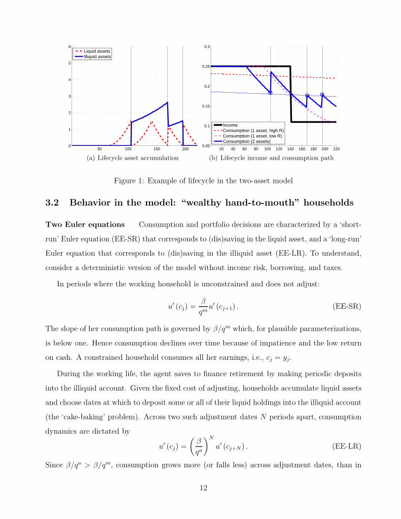
Figure 1: Example of lifecycle in the two-asset model

3.2 Behavior in the model: “wealthy hand-to-mouth” households

Two Euler equations Consumption and portfolio decisions are characterized by a ‘short-

run’ Euler equation (EE-SR) that corresponds to (dis)saving in the liquid asset, and a ‘long-run’

Euler equation that corresponds to (dis)saving in the illiquid asset (EE-LR). To understand,

consider a deterministic version of the model without income risk, borrowing, and taxes.

In periods where the working household is unconstrained and does not adjust:

u′ (cj) =β

qmu′ (cj+1) . (EE-SR)

The slope of her consumption path is governed by β/qm which, for plausible parameterizations,

is below one. Hence consumption declines over time because of impatience and the low return

on cash. A constrained household consumes all her earnings, i.e., cj = yj.

During the working life, the agent saves to finance retirement by making periodic deposits

into the illiquid account. Given the fixed cost of adjusting, households accumulate liquid assets

and choose dates at which to deposit some or all of their liquid holdings into the illiquid account

(the ‘cake-baking’ problem). Across two such adjustment dates N periods apart, consumption

dynamics are dictated by

u′ (cj) =

(

β

qa

)N

u′ (cj+N) . (EE-LR)

Since β/qa > β/qm, consumption grows more (or falls less) across adjustment dates, than in

12

between adjustments.

During retirement, the household faces a ‘cake-eating’ problem, where optimal decisions

closely resemble those in Romer (1986). Consumption in excess of pension income is financed by

making periodic withdrawals from the illiquid account. Between each withdrawal, the household

runs down its liquid holdings and consumption falls according to (EE-SR). The withdrawals

are timed to coincide with the period where cash is exhausted. Across withdrawals, equation

(EE-LR) holds.14

Figure 1 shows consumption and wealth dynamics in an example where an agent with

logarithmic utility starts her working life with zero wealth, receives a constant endowment

while working and a lower endowment when retired.15 Panel (a) shows that the agent in this

example chooses to adjust his illiquid account at only three points in time: one deposit while

working, and two withdrawals in retirement. In between, the value of the illiquid account grows

at rate 1/qa. Panel (b) shows her associated income and consumption paths. In the same panel,

we have also plotted the paths for consumption arising in the two versions of the corresponding

one-asset model: one with the ‘short-run’ interest rate 1/qm, and one with the ‘long-run’ rate

1/qa. The sawed pattern for consumption that arises in the two-asset model is a combination

of the short-run and long-run behavior: between adjustment dates the consumption path is

parallel to the path in the one-asset model with the low return; while across consumption

dates, the slope is parallel to consumption in the one-asset model with the high return. Finally

note that, under this parameterization, the young agent is constrained for the initial phase of

her working life, when her net worth is zero.

Endogenous ‘hand-to-mouth’ behavior Figure 2 illustrates how the model can fea-

ture households with positive net worth who consume their income every period: the “wealthy

hand-to-mouth” agents. The parameterization is the same as in Figure 1, except for a higher

return on the illiquid asset Ra. This higher return leads to stronger overall wealth accumula-

tion. Importantly, rather than increasing the number of deposits during the working life, the

household changes the timing of its single deposit. The single deposit into the illiquid account

14In this example, our problem during retirement with no discounting, log utility, and the transaction costexpressed in utility terms would coincide with Romer (1986) and withdrawal dates would be equidistant, subjectto the ‘integer problem’ intrinsic in the discrete-time formulation.

15To make this example as stark as possible, we impose a very large transaction cost.

13

50 100 150 2000

1

2

3

4

5

6

Liquid assetsIlliquid assets

(a) Lifecycle asset accumulation

20 40 60 80 100 120 140 160 180 200 2200.05

0.1

0.15

0.2

0.25

0.3

IncomeConsumption

(b) Lifecycle income and consumption path

Figure 2: Example of lifecycle of a ‘wealthy hand-to-mouth’ agent in the two-asset model

is now made earlier in life in order to take advantage of the high return for a longer period

(compare the left panels across Figures 1 and 2). Thus, instead of being constrained at the

beginning of the life cycle, the household optimally chooses to hold zero liquid assets in the

middle of the working life, after its deposit, while the illiquid asset holdings are positive and are

growing in value. Intuitively, since her net worth is large, this household would like to consume

more than her earnings flow, but the transaction cost dissuades her from doing it. This is a

household that, upon receiving the rebate, will consume a large part of it and, upon the news

of the rebate, cannot increase her expenditures without making a costly withdrawal from her

illiquid account.16

Why would households choose to consume all of their earnings every period and deviate

from the optimal consumption path imposed by the short-run Euler equation EE-SR, even for

long periods of time? The answer is that households are better off taking this welfare loss

than smoothing consumption because the latter option entails either (i) paying the transaction

cost more often to withdraw cash when needed to smooth shocks; or (ii) accumulating more

liquid wealth for precautionary reasons hence foregoing the high return on the illiquid asset

(and, therefore, the associated higher level of consumption). This observation is reminiscent of

16As discussed in the Introduction, the model by Campbell and Hercowitz (2009) also features ‘wealthyconstrained’ agents. However, their mechanism is different and, even though it is consistent with high MPC outof transitory shocks, would not be capable of generating large MPC out of anticipated income changes or largerebate coefficients.

14

Cochrane’s (1989) insight that, in a representative agent model with reasonable risk aversion,

the utility loss from setting consumption equal to income is very small.17

4 Calibration

We now present a calibration of the model without credit (m = 0) and without heterogenous

earnings slopes (ψi = 0) . In Section 6 we analyze these extensions of the model.

Demographics and preferences Decisions in the model take place at a quarterly fre-

quency. Households begin their active economic life at age 22 (j = 1) and retire at age 60

(Jw = 152). The retirement phase lasts for 20 years (Jr = 80). We assume a unitary intertem-

poral elasticity of substitution (γ = 1) and we calibrate the discount factor β to replicate median

illiquid wealth in the SCF (see below).18

Earnings heterogeneity We estimate the parameters of the earnings process (common

life-cycle profile, initial variance of earnings, and variance of earnings shocks) through a mini-

mum distance algorithm that targets the empirical covariance structure of household earnings

constructed from the Panel Study of Income Dynamics (PSID). Specifically, from the PSID we

select a sample of households with heads 22-59 years old in 1969-1996, following the same crite-

ria as in Heathcote, Perri, and Violante (2010). We construct the empirical mean age-earnings

profile and covariance functions in levels and first differences, exploiting the longitudinal di-

mension of the data. We simulate the process in (3) at a quarterly frequency, also allowing for

an i.i.d. shock, and aggregate quarterly earnings into annual earnings. From the implied annual

earnings we construct the model counterpart of the empirical moments and minimize the dis-

tance between the two set of moments. We interpret the transitory component as measurement

17See also Browning and Crossley (2001) for a similar calculation in the context of the life-cycle model ofconsumption.

18In the literature on quantitative macroeconomic models with heterogeneous households and incompletemarkets there are two approaches to calibrating the discount factor. The first is to match median wealth (e.g.,Carroll, 1992, 1997). The second is to match aggregate wealth (e.g., Aiyagari, 1994; Rios-Rull, 1995; Kruselland Smith, 1998). There is a trade off in this choice. Matching median wealth allows one to reproduce moreclosely the wealth distribution, with the exception of the upper tail. Matching mean wealth allows one to fullyincorporate equilibrium effects on prices, at the cost of overstating wealth holdings and, therefore, understatingthe MPC for a large fraction of households (due to the concavity of the consumption function, see Carroll andKimball, 1996). Since, for the question at hand, matching the liquid and illiquid wealth holdings of households,as well as their MPC, the bottom half of the distribution is far more important than price effects, here wechoose the former approach.

15

error in earnings and hence, in simulations, we abstract from it.

Households’ portfolio data Our data source is the 2001 wave of the SCF, a triennial cross-

sectional survey of the assets and debts of US households. For comparability with the CEX

sample in JPS (2006), we exclude the top 5% of households by net worth. Average labor income

for the bottom 95% is $52,696, a number close to the one reported by JPS (2006, Table 1).19

Our definition of liquid assets comprises: money market, checking, savings and call accounts

plus directly held mutual funds, stocks, bonds, and T-Bills net of revolving debt on credit card

balances.20 All other wealth, with the exception of equity held in private businesses, is included

in our measure of illiquid assets. It comprises housing net of mortgages and home equity loans,

vehicles net of installment loans, retirement accounts (e.g., IRA, 401K), life insurance policies,

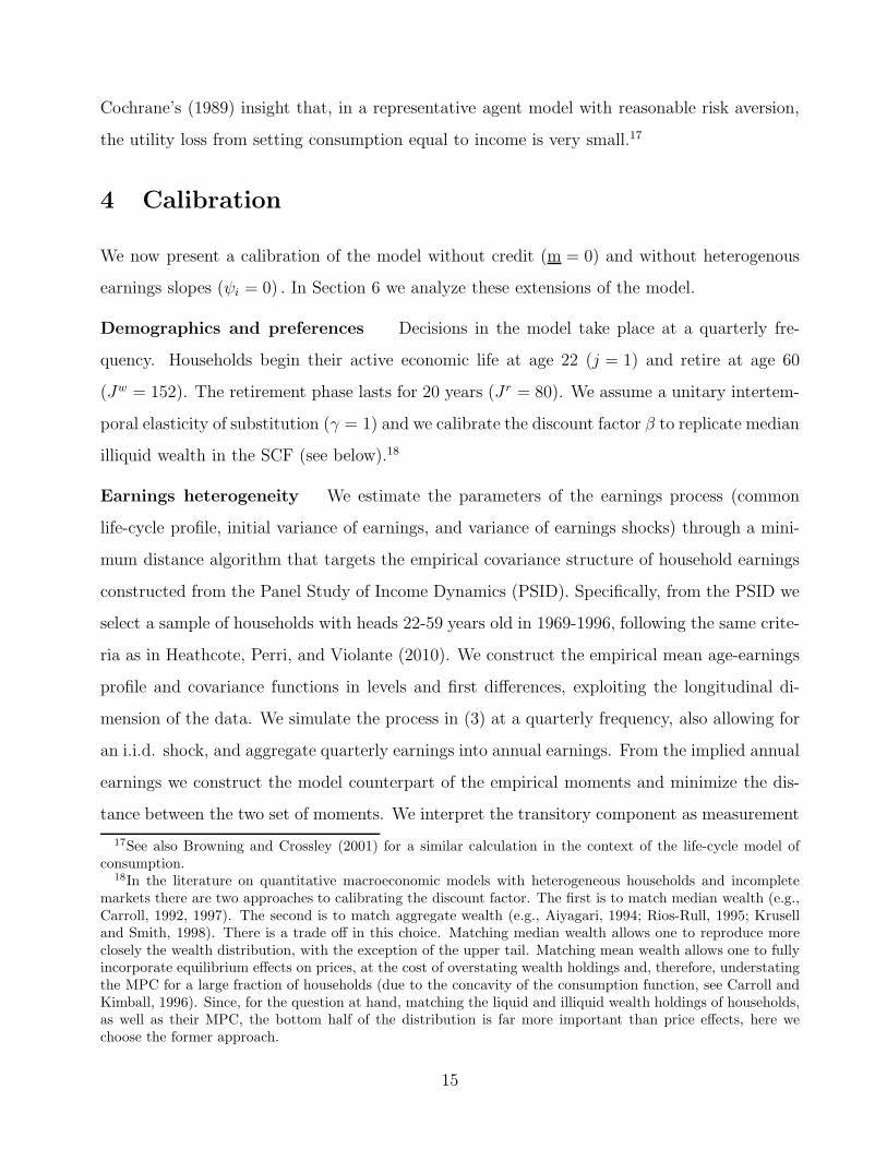
CDs, and saving bonds. Table 2 reports some descriptive statistics.

The data provide overwhelming evidence that the majority of household wealth is held in

(what we call) illiquid assets. For example, the median and mean of the liquid asset distribution

are $2,700, and $30,531, compared with $70,000, and $133,932 for the illiquid asset distribution.

Figure 3(a) shows the evolution of illiquid and liquid wealth over the lifecycle. It is clear

that the bulk of the life-cycle saving over the working life takes place in illiquid wealth, whereas

liquid wealth is fairly constant.

Measuring hand-to-mouth households in the SCF An implication of these low hold-

ings of liquid wealth is that a number of households are likely to be hand-to-mouth, i.e., they

hold liquid assets only because earnings are paid as cash and because of a mismatch in the

timing of consumption and earnings within a pay period, not because they save across peri-

ods. To measure the fraction of these hand-to-mouth households, one must take a stand on

the frequency of pay dates. If households are surveyed at the midpoint of a pay-period, and if

19In our definition of household labor income, we included unemployment and disability insurance, TANF,and child benefits.

20The SCF asks the following questions about credit card balances: (i) “How often do you pay on yourcredit card balance in full?” Possible answers are: (a) Always or almost always; (b) Sometimes; or (c) Almostnever. (ii) “After the last payment, roughly what was the balance still owed on these accounts?” From thefirst question, we identify households with revolving debt as those who respond (b) Sometimes or (c) AlmostNever. We then use the answer to the second question, for these households only, to compute statistics aboutcredit card debt. This strategy (common in the literature, e.g., see Telyukova, 2011) avoids including, as debt,purchases made through credit cards in between regular payments.

16

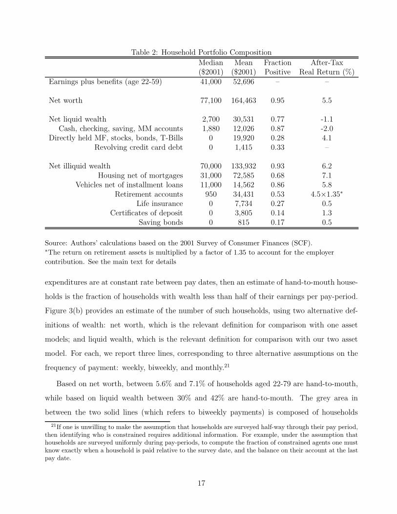
Table 2: Household Portfolio Composition

Median Mean Fraction After-Tax($2001) ($2001) Positive Real Return (%)

Earnings plus benefits (age 22-59) 41,000 52,696 – –

Net worth 77,100 164,463 0.95 5.5

Net liquid wealth 2,700 30,531 0.77 -1.1Cash, checking, saving, MM accounts 1,880 12,026 0.87 -2.0

Directly held MF, stocks, bonds, T-Bills 0 19,920 0.28 4.1Revolving credit card debt 0 1,415 0.33 –

Net illiquid wealth 70,000 133,932 0.93 6.2Housing net of mortgages 31,000 72,585 0.68 7.1

Vehicles net of installment loans 11,000 14,562 0.86 5.8Retirement accounts 950 34,431 0.53 4.5×1.35∗

Life insurance 0 7,734 0.27 0.5Certificates of deposit 0 3,805 0.14 1.3

Saving bonds 0 815 0.17 0.5

Source: Authors’ calculations based on the 2001 Survey of Consumer Finances (SCF).∗The return on retirement assets is multiplied by a factor of 1.35 to account for the employer

contribution. See the main text for details

expenditures are at constant rate between pay dates, then an estimate of hand-to-mouth house-

holds is the fraction of households with wealth less than half of their earnings per pay-period.

Figure 3(b) provides an estimate of the number of such households, using two alternative def-

initions of wealth: net worth, which is the relevant definition for comparison with one asset

models; and liquid wealth, which is the relevant definition for comparison with our two asset

model. For each, we report three lines, corresponding to three alternative assumptions on the

frequency of payment: weekly, biweekly, and monthly.21

Based on net worth, between 5.6% and 7.1% of households aged 22-79 are hand-to-mouth,

while based on liquid wealth between 30% and 42% are hand-to-mouth. The grey area in

between the two solid lines (which refers to biweekly payments) is composed of households

21If one is unwilling to make the assumption that households are surveyed half-way through their pay period,then identifying who is constrained requires additional information. For example, under the assumption thathouseholds are surveyed uniformly during pay-periods, to compute the fraction of constrained agents one mustknow exactly when a household is paid relative to the survey date, and the balance on their account at the lastpay date.

17

30 40 50 60 70 800

50

100

150

200

250

300

350

Age

Dol

lars

(00

0’s)

Median Illiquid WealthMedian Liquid Wealth

(a) Median liquid and illiquid wealth (SCF)

30 40 50 60 70 800

0.1

0.2

0.3

0.4

0.5

0.6

Age

Fra

ctio

n of

Hou

seho

lds

Constrained in terms of net worthConstrained in terms of liquid wealth

(b) Hand-to-mouth households (SCF): – monthlypay; - biweekly pay; -. weekly pay

Figure 3: Liquid and illiquid wealth over the life-cycle in the data (2001 SCF)

who have positive illiquid wealth but do not carry positive balances of liquid assets between

pay periods. These are the empirical counterpart of the ‘wealthy hand-to-mouth’ agents in

our model. Note that this last group of households, which represents a sizeable fraction of the

population (between 24% and 35%), is only visible through the lenses of the two-asset model.

From the point of view of the standard one asset model, these are households with positive net

worth, hence unconstrained.

These findings are consistent with recent survey evidence in Lusardi, Schneider, and Tufano

(2011) showing that almost one third of US households would “certainly be unable to cope

with a financial emergency that required them to come up with $2,000 in the next month.”

The authors also report that, among those giving that answer, a high proportion of individuals

are at middle class levels of income. Similarly, Broda and Parker (2011) document, from the

AC Nielsen Homescan database, that almost 40% of households report that they do not have

“at least two months of income available in cash, bank accounts, or easily accessible funds ”.

Asset returns To measure returns on the various asset classes, we focus on the period 1960-

2009. All of the following returns are expressed in annual nominal terms. We set the nominal

return on checking accounts to zero and the return on savings accounts, T-Bills and savings

bonds to the interest rate on 3-month T-Bills, which was 5.3% over this period (FRB database).

For equities, we use Center for Research in Security Prices (CRSP) value-weighted returns,

18

assuming dividends are reinvested, and obtain an annualized nominal return of 11.1%.22 The

SCF reports the equity share for directly held mutual funds, stocks and bonds and for retirement

accounts, which allows us to apply separate returns on the equity and bond components of each

saving instrument. An important incentive to save in retirement accounts is the employer’s

matching rate. Over 70% of households in our sample with positive balance on their retirement

account have employer-run retirement plans. The literature on this topic finds that, typically,

employers match 50% of employees’ contributions up to 6% of earnings, but the vast majority

of employees do not contribute above this threshold (e.g., Papke and Poterba, 1995). As a

result, we raise the return on retirement accounts by a factor of 1.35.23

For housing, we follow Favilukis, Ludvigson, and Van Niewerburgh (2010). We measure

housing wealth for the household sector from the Flow of Funds, and housing consumption

from the National Income and Products Accounts. The return for year t is constructed as

housing wealth in the fourth quarter of year t plus housing consumption over the year minus

expenses in maintenance and repair divided by housing wealth in the fourth quarter of year

t− 1.24 We subtract population growth in order to correct for the growth in housing quantity.

We also subtract the average property tax, 1% (Tax Foundation, 2011). As a result, we obtain

an average annual nominal return of 13.2%.25

Given the absence of data on the service flow from vehicles (autos, trucks and motorcycles),

we adopt a user cost approach to calculate the return on vehicles. The sum of the interest rate

on T-Bills plus the rate of economic and physical depreciation (available from the BEA) yields

an annual nominal return of 11.6%. For saving bonds and life insurance (assuming actuarially

fair contracts for the latter) we use the return on T-Bills, and for CDs we obtain a nominal

return of 6.3% (FRB database).

22After inflation (4.1% over this period), the real return is 7%. Favilukis, Ludvigson, and Van Niewerburgh(2010, Table 5), whose calculations we follow, report returns between 7.9% (1953-2008) and 6.6% (1972-2008).

23Since we do not model explicitly the tax-deferred treatment of retirement accounts, we somewhat underes-timate the effective return on this saving vehicle. See Huntley and Michelangeli (2011).

24Our estimate of expenses in improvement and repair is based on a comprehensive study on housing compiledby the Joint Center for Housing Studies (2011). Figure 2 reports that these expenses amount to roughly 40%of total residential investment expenditures.

25After inflation, the real return is 9.1%. Favilukis et al. (2010, Table 5) report returns between 9.8% (1953-2008) and 9.9% (1972-2008). They also report a housing return of 9.1% (1972-2008) computed based on therepeat-sale Freddie Mac Conventional Mortgage House Price index for purchases only (Freddie Mac) and onthe rental price index for shelter (BLS).

19

We apply these nominal returns to each household portfolio in the SCF and compute average

returns in the population. The implied average nominal return on illiquid wealth is 12.1% and

on liquid wealth is 3.8%. Finally, we set the annual inflation rate to 4.0 percent (the average

over this period is 4.1). After inflation and taxes (see below), the after-tax real returns on

liquid and illiquid wealth are 6.2% and -1.1%, respectively. The final after-tax real returns on

liquid and illiquid wealth by category are reported in Table 2.

Initial asset positions We use observed wealth portfolios of SCF households aged 20 to

24 to calibrate the age j = 0 initial conditions for assets in the model. We divide this group

into fifteen sub-groups based on their earnings and calculate 1) the fraction with zero holdings,

and 2) the median liquid wealth, illiquid wealth, and net worth in each sub-group, conditional

on positive holdings. When we simulate life-cycles in the model, we create the same sub-groups

based on the initial earnings draw. Within each sub-group, we initialize a fraction of agents

with zero assets, and the rest with the corresponding median holdings of liquid and illiquid

wealth.

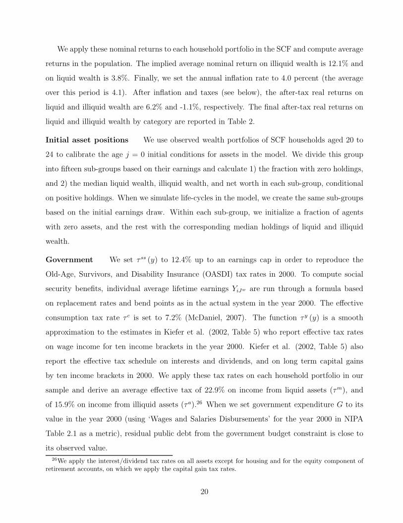
Government We set τ ss (y) to 12.4% up to an earnings cap in order to reproduce the

Old-Age, Survivors, and Disability Insurance (OASDI) tax rates in 2000. To compute social

security benefits, individual average lifetime earnings YiJw are run through a formula based

on replacement rates and bend points as in the actual system in the year 2000. The effective

consumption tax rate τ c is set to 7.2% (McDaniel, 2007). The function τ y (y) is a smooth

approximation to the estimates in Kiefer et al. (2002, Table 5) who report effective tax rates

on wage income for ten income brackets in the year 2000. Kiefer et al. (2002, Table 5) also

report the effective tax schedule on interests and dividends, and on long term capital gains

by ten income brackets in 2000. We apply these tax rates on each household portfolio in our

sample and derive an average effective tax of 22.9% on income from liquid assets (τm), and

of 15.9% on income from illiquid assets (τa).26 When we set government expenditure G to its

value in the year 2000 (using ‘Wages and Salaries Disbursements’ for the year 2000 in NIPA

Table 2.1 as a metric), residual public debt from the government budget constraint is close to

its observed value.

26We apply the interest/dividend tax rates on all assets except for housing and for the equity component ofretirement accounts, on which we apply the capital gain tax rates.

20

4.1 Modelling the 2001 tax rebate, tax reform, and recession

Tax rebate We assume that the economy is in steady state in 2001:Q1. The rebate checks

are then randomly sent out to half the eligible population in 2001:Q2, and to the other half

in 2001:Q3. We set the rebate size to $500 based on JPS (2006) who report that the average

rebate check was $480 per household.

There are different views that one could plausibly take about the timing of when the rebate

enters households’ information sets. At one extreme, households become fully aware of the

rebate when the bill is discussed in Congress and enacted. This scenario implies the news

arriving in 2001:Q1. Under this timing, the check is fully anticipated by both groups. At

the other extreme, one could assume that households became aware of the rebate only after

receiving their own check: under this assumption, both groups of households treat the rebate

as a surprise. In our baseline, we take an intermediate position, i.e., all households learn about

the rebate when the first set of Treasury checks are received, in 2001:Q2. Under this timing,

the check was fully anticipated only by the second group who received the check in 2001:Q3.

We explore the two alternative timing assumptions in Section 6. We assume throughout that

the news/check reaches households before the consumption/saving and adjustment decisions

for that quarter.

Tax reform The 2001 rebate was part of a broader tax reform which, beyond decreasing the

lowest rate, also reduced all other marginal rates by roughly 3% or more. We construct the

sequence of effective tax schedules based on Kiefer et al. (2002).27 Most of these changes were

planned to be phased in gradually over the five years 2002:Q1-2006:Q1 and to ‘sunset’ in 2011.

It turned out that instead of sunsetting, the tax cuts were further extended. We consider two

scenarios regarding the ‘sunset’ clause: (i) households believe that the tax system will revert to

its pre-reform state at the end of ten years; and (ii) households act as if the change in the tax

system is permanent after the reform is fully phased in. A tax reform is defined as a sequence

of tax schedules {Tt}t∗∗

t=t∗ which is announced, jointly with the rebate, in 2001:Q2. Date t∗, the

first quarter of the change in the tax code, is 2002:Q1. Date t∗∗, the last quarter of the change

27Kiefer et al. (2002, Table 5) report the pre and post reform income tax rates, and describe the timing ofthe reduction in the various brackets (page 90).

21

in the tax code, is 2006:Q1 in absence of sunset, and 2011:Q1 when the tax reform sunsets as

originally legislated.

Recession To model the downturn of 2001, we assume that in 2001:Q2 households become

aware that they are entering a recession. At this time they learn that their labor income will

fall linearly for the next three quarters, generating a cumulative drop of 1.5%, and will then

fully recover over the following eight quarters.28

Transition In 2001:Q2 the economy begins undergoing transitional dynamics. We start by

assuming that the government finances the rebate program by increasing debt for ten years, and

then repays the rebate outlays and the accumulated interest on the new debt by introducing a

permanent proportional tax on earnings. In our benchmark calibration, the required additional

tax rate is around 0.05%.29

5 Quantitative analysis of the 2001 tax rebate

We start by studying a baseline economy where the tax rebate occurs in isolation. Next, we

incorporate the tax reform and recession. We analyze the model economy for values of the

transaction cost κ ranging from zero to $3,000. The case κ = 0 corresponds to the standard

one-asset model. At κ = 0, we set β to reproduce median net worth, and we set the interest

rate to the average return on net worth in the SCF data (see Table 2).30 For each value of

κ > 0, we re-calibrate β to match median holdings of illiquid wealth.31

Baseline results To fix ideas, it is useful to start from the one-asset economy with κ = 0.

When we compute the rebate coefficient exactly as in JPS (2006) –i.e., we run regression (1)

on simulated panel data– the estimated rebate coefficient is only 1.8%. The vast majority of

28The NBER dates the 2001 recession as starting in March 2001 and ending in November 2001. The magnitudeof the downturn and the duration of its recovery are calibrated from the ‘Wages and Salaries Disbursments’series in NIPA Table 2.1.

29We experimented by shortening the phase during which the government uses debt up to one year and foundnearly identical results. There are two reasons. First, the financing scheme affects equally the treatment andthe control group. Second, the behavior of constrained households is unaffected by future rises in taxes.

30This latter choice has no bearing on the findings since the discount factor is always calibrated to generatethe same amount of net worth. When we set the interest rate to the calibrated value of Rm or Ra, we foundvirtually identical results.

31The annualized values of β range between 0.950 and 0.956. Hence, our results are not driven by implausiblylow discount factors which make households highly impatient.

22

households in this model hold enough net worth to save the bulk of the rebate, upon its receipt.

Moreover, the response to the news and to the check itself are virtually identical for this group,

as predicted by standard consumption theory. The action comes entirely from the constrained

agents, most of which are very young (below age 35): those in the treatment group have a

high MPC, while those in the control group do not respond at all. In our calibration, only 3

% of households have zero net worth and are hand-to-mouth, which explains the small rebate

coefficient.32

We now move to the two-asset model with κ > 0. Figure 4(a) shows that the fraction of

households adjusting (i.e., accessing the illiquid account to withdraw or deposit) falls with the

size of the transaction cost κ. As illustrated in the simulations of Section 3, retirees adjust

more often than working-age households because they finance their consumption largely by

withdrawing from the illiquid account. Holdings of liquid wealth increase with the transaction

cost (Figure 4(b)), because when κ is larger households deposit into/withdraw from the illiquid

account less often and carry larger balances of liquid assets. However, even for large transaction

costs, median liquid wealth remains small, around $1,500.33

A corollary of the skewed liquid wealth distribution in Figure 4(b) is that a substantial

fraction of agents do not carry any balances of liquid assets across periods (i.e., do not use cash

to save). In the model, there are two types of such agents. Some agents have zero liquid assets

at the end of the period because they just made a deposit or they will make a withdrawal next

period. Others have zero liquid assets at the end of the period because they are hand-to-mouth

and consume their earnings every period. Figure 4(c) plots the fraction of households in the

latter group, the hand-to-mouth consumers, and divides them into those who also have zero

illiquid wealth and those with positive illiquid wealth. The size of both groups is increasing in κ.

32As reported in Figure 3(b), in the 2001 SCF data this fraction is around 6%. Hence, even though the modelat κ = 0 slightly underestimates this fraction, there is essentially no scope for the one asset model to generatesignificant rebate coefficients, while remaining consistent with SCF data on the distribution of net worth.

33One may be surprised that optimal holdings of liquid wealth are so small, given the presence of plausiblycalibrated earnings risk. However, with highly persistent shocks, there is little incentive to hold liquid wealthfor precautionary reasons, a well known result in the literature. This is for two reasons. First, the opportunitycost of holding cash is very high, since Ra is large. Second, households can always withdraw (at a cost) fromthe illiquid account in the event of a large negative shock. This view of earnings risk is consistent with theobserved distribution of liquid wealth holdings: had we allowed for a large transitory earnings component, house-holds would hold counterfactually high quantities of liquid assets, and, accordingly, would have low marginalpropensities to consume out of the rebate.

23

0 500 1000 1500 2000 2500 30000

20

40

60

80

100

Fixed Cost ($)

Fra

ctio

n A

djus

ting(

%)

WorkersRetirees

(a) Fraction of households adjusting

0 500 1000 1500 2000 2500 30000

2000

4000

6000

8000

10000

12000

Fixed Cost ($)

Liqu

id W

ealth

+ 0

.25

* M

onth

ly E

arni

ngs

($)

25th pctileMedian75th pctile

(b) Distribution of liquid wealth

0 500 1000 1500 2000 2500 30000

10

20

30

40

50

Fixed Cost ($)

Hand−to−mouth, no illiquid wealthHand−to−mouth, positive illiquid wealth

(c) Fraction of hand-to-mouth households

0 500 1000 1500 2000 2500 300010

15

20

25

30

35

40

Qua

rter

s

Fixed Cost ($)

(d) Mean length of hand-to-mouth spells

Figure 4: Features of two-asset model, by transaction cost

As shown in Figure 4(d), the average length of spells in which hand-to-mouth households hold

zero liquid assets and consume their income is also growing with the level of the transaction

cost. Intuitively, a large value for κ makes it less likely that the household will withdraw from

the illiquid account to smooth large negative earnings shocks.

In what follows, we often focus on the range $500-$1,000 for the transaction cost: in this

range, (i) the fraction of households that adjust each quarter is 15%-20% (4%-8% among workers

and 35%-45% among retirees); (ii) median holdings of liquid wealth are just below their data

counterpart in Table 2; and (iii) the fraction of hand-to mouth consumers is in line with the

empirical estimates of Figure 3.

24

0 500 1000 1500 2000 2500 3000−5

0

5

10

15

20

25R

ebat

e C

oeffi

cien

t (%

)

Fixed Cost ($)

(a) Rebate coefficient

0 500 1000 1500 2000 2500 3000

0

10

20

30

40

50

Fixed Cost ($)

Mar

gina

l Pro

pens

ity to

Con

sum

e (%

)

Hand−to−mouth agentsNon hand−to−mouth agents

(b) Average marginal propensity to consume

Figure 5: Rebate coefficient and marginal propensity to consume, by transaction cost

Figure 5(a) displays the rebate coefficient in the model for different levels of the transaction

cost. The rebate coefficient grows steadily from 1.8% when κ = 0 (the one-asset model) to

21% when κ = $3, 000. For transaction costs in the range $500-$1,000, the rebate coefficient

is around 15%, or 8 times higher than its one-asset model counterpart. Figure 5(b) shows the

marginal propensities to consume (MPC) out of the fiscal stimulus payment for two groups

of households: those who are hand-to-mouth and those who are not. Note how, for the latter

group, the average MPC is close to zero, while for the former group it is around 45%. Therefore,

most of the households in the model behave exactly as predicted by the PIH and have zero MPC.

The high rebate coefficients are driven by constrained households, and the two-asset model

generates a larger fraction of hand-to-mouth consumers, some of which hold sizeable quantities

of illiquid assets. Such households have significant MPC out of the rebate check (when they

are in the treatment group) and do not respond to the news of the check (when they are in

the control group). As a back of the envelope calculation, the 15% rebate coefficient arises as a

weighted average of zero MPC for 2/3 of the population and 45% MPC for the remaining 1/3

in the treatment group. In the control group, both hand-to-mouth and unconstrained agents

have zero MPC.

For low transaction costs, marginal propensities to consume out of moderate income changes

(and hence rebate coefficients) can be negative. When transaction costs are low enough, upon

25

0 500 1000 1500 2000 2500 3000−5

0

5

10

15

20

25

30

35R

ebat

e C

oeffi

cien

t (%

)

Fixed Cost ($)

No tax reformTax reform without sunsetTax reform with sunset

(a) Rebate coefficient with tax reform

0 500 1000 1500 2000 2500 3000−5

0

5

10

15

20

25

30

35

Reb

ate

Coe

ffici

ent (

%)

Fixed Cost ($)

No tax reform, No recessisionTax reform, No recessionTax reform, With recession

(b) Rebate coefficient with recession

Figure 6: Effect of tax reform and recession on rebate coefficient, by transaction cost

receiving the rebate agents may choose to anticipate the adjustment decision and save the

rebate, together with their current holdings of cash, into the illiquid account. As a result,

they save more than the rebate amount (which explains the negative MPC in Figure 5(b)) and

consume less than the control group (which explains the negative rebate coefficient in Figure

5(a)).

Tax reform and recession Figure 6(a) shows that the consumption responses to the tax

rebate are substantially higher when the full tax reform is modeled. On average, the rebate

coefficient increases by 7-8 percentage points. The reason is that the substantial reduction

in future tax liabilities leads to a rise in the desired level of lifetime consumption. Since a

substantial fraction of households (poor and wealthy) are constrained in terms of liquid wealth,

the rebate enables such households to start consuming out of this additional future income

earlier than they would otherwise be able to.34 As is clear from the figure, our finding is robust

to whether the sunset clause is implemented or not.

A similar logic applies when we add the recession to the tax rebate experiment. Figure 6(b)

shows that allowing for the fact that the economy was undergoing a recession at the time of

the rebates adds roughly 3 percentage points to the rebate coefficient. Overall, in the range

34When adding the tax reform, the economy with κ = 0 also yields a higher rebate coefficient (see Figure6(a)), because the effect we describe does apply there as well. However, quantitatively, the additional kick ofthe tax reform is insignificant in the one-asset model because the number of constrained households is so small.

26

0.1

.2.3

.4F

ract

ion

of H

ouse

hold

s

0 .2 .4 .6 .8 1Rebate Coefficient

(a) Distribution of rebate coefficients in thepopulation

020

000

4000

060

000

8000

0M

edia

n E

arni

ngs

0 20 40 60 80 100Percentile of Rebate Coefficient Distribution

(b) Median earnings by percentile of rebate co-efficient distribution

Figure 7: Heterogeneity in rebate coefficients in the model (κ = $750)

$500-$1,000 for κ, the model generates a rebate coefficient between 22% and 29%, in line with

the estimates of Table 1.

5.1 Further implications on consumption responses

Cochrane’s (1989) observation that there may be only small welfare differences between alter-

native consumption behavior when reacting to small transitory income shocks means that it is

especially useful to investigate additional implications of our model, a point also raised by Card

et al. (2007), and Chetty (2011). Our model has a number of implications about households’

consumption responses that can be compared to the data. We explore: 1) the heterogeneity in

consumption responses across households; 2) their correlation with households’ liquid wealth; 3)

their size-asymmetry; and 4) their state-dependence. When, in order to present more detailed

features of our model, it is necessary to select a specific value for κ, we choose κ = $750. In the

presence of the tax reform and recession, this value corresponds to a rebate coefficient of 27%.

Heterogeneity Misra and Surico (2011) apply quantile regression techniques to the same

data set as JPS (2006) to study cross-sectional heterogeneity in rebate coefficients. They

conclude that there is a large amount of heterogeneity in consumption responses. There are two

main findings. First, the distribution of consumption responses is bimodal, with around 40% of

households saving all of the rebate, and another sizeable group of households spending a high

27

fraction of the rebate.35 Second, high income households are disproportionately concentrated

in the two tails of the distribution of consumption responses.36 Figure 7 shows that our model

can broadly reproduce these findings.

Figure 7(a) plots a histogram of rebate coefficients for the working age population, in which

the bimodal nature is stark. The bimodality arises because of the coexistence of a substantial

fraction of (wealthy) hand-to-mouth consumers together with unconstrained agents who fully

save the rebate as predicted by standard theory. Figure 7(b) plots median earnings in each

quantile of the cross-sectional distribution of the consumption responses. The reason why

there are high earnings households at both ends of the distribution is that some of them are

unconstrained and some are wealthy hand-to-mouth. The former are income-rich but their

expected earnings growth is low, the latter are income-rich but their expected earnings profile

is steep, which makes the liquidity constraint more likely to bind. Moreover, because the rebate

is a lump sum, among constrained agents the income-richest have the highest MPC.

Correlation with liquid wealth JPS (2006) estimate rebate coefficients for sub-groups

of households with different amounts of liquid assets. They find that households in the bottom

half of the distribution have substantially larger consumption responses. These effects are

imprecisely estimated, though, for two reasons. First, the sample becomes very small when

divided into sub-groups. Second, the asset data in the CEX must be viewed with extreme

caution, due to the large amount of item non-response. For example, JPS (2006) have data

on liquid wealth for less than half of the sample, and hence it is likely that respondents are a

highly selected sub-sample. Misra and Surico (2011) also conclude that liquid assets are not

strongly correlated with the size of the consumption response: they identify high liquid wealth

35A complementary source of evidence comes from SS (2003a, 2003b) who added an ad-hoc module to theMichigan Survey of Consumers to assess the impact of the rebate. This survey asked households what theywould do with their rebate check. 22 percent of respondents said they would mostly spend it, while the restsaid they would mostly save it or repay debt. From these studies, we can infer that the average estimate fromJPS is likely to be the outcome of very high MPC among a relatively small group of households and verysmall (or zero) MPC among the majority of the population. PSJM (2011) validate this survey-based finding bydocumenting that CEX households who report that they mostly consumed the 2008 rebate had consumptionresponses almost twice as large as those households who report that they mostly saved it.

36This second finding is not inconsistent with (and could potentially explain) the result reported by JPS(2006) that, when splitting the population into three income groups, differences in rebate coefficient acrossgroups are not statistically significant. Similarly, SS (2003a, 2003b) find no evidence of higher spending ratesamong low income households.

28

0 500 1000 1500 2000 2500 3000−5

0

5

10

15

20

25

Reb

ate

Coe

ffici

ent (

%)

Fixed Cost ($)

$500 rebate$1000 rebate $2000 rebate$5000 rebate

Figure 8: Rebate coefficients by size of the stimulus payment

households at both ends of the distribution of rebate coefficients.

These results are not inconsistent with our model. In the model, there are some high liquid

wealth households who are not constrained and consume little out of the rebate, and others

(with high income and high expected income growth) who are constrained and have a large

MPC out of the rebate. This feature of the model explains why, empirically, the relationship

between rebate coefficients and the level of liquid wealth is statistically weak.

The model’s sharpest prediction is that households with low liquid wealth to earnings ratios

have larger consumption responses. Broda and Parker (2011) exploit the AC Nielsen Homescan

database, a sample fifty times larger than the CEX, to study the consumption response to the

fiscal stimulus payment of 2008. They ask households “In case of an expected decline in income

or increase in expenses, do you have at least two months of income available in cash, bank

accounts, or easily accessible funds?” Hence their liquid wealth variable is relative to earnings.

They split households in two groups and find very strong (and statistically significant) evidence

that households with a low ratio of liquid assets to income spend at least twice as much as the

average household, precisely as predicted by our model.37

Size asymmetry Hsieh (2003) shows that the same CEX consumers who ‘overreact’ to the

37Souleles (1999) studies the consumption response to anticipated tax refunds (whose median size is around$560 (Table 1). When the sample is split between low and high liquid wealth-earnings ratio households, theformer group is found to have statistically significant larger responses to the refund (Table 4).

29

2001 tax rebates, respond very weakly to payments received from the Alaskan Permanent Fund.

These payments are, on average, much larger than the rebate we examined (around $2,000 per

household). Browning and Collado (2001) document similar evidence from Spanish survey data:

workers who receive anticipated double-payment bonuses (hence, again, large amounts) in the

months of June and December do not alter their consumption growth significantly in those

months. One interpretation of these results is that, although households spend large fractions

of small anticipated shocks, they predominantly save large anticipated shocks.

Figure 8 shows how the propensity to consume the rebate declines when the size of the

rebate is increased above $500, as a function of κ. In the baseline environment with a $750

transaction cost, the rebate coefficient drops by almost a factor of three (from 16% to 6%) as

the size of the stimulus payment increases from $500 to $2,000. A large enough rebate loosens

the liquidity constraint, and even constrained households will find it optimal to save a portion

of their payment.38 Moreover, for rebates that are sufficiently high relative to the transaction

cost, many working households will choose to pay the transaction cost and make a deposit

upon receipt of the rebate. But, since adjusting households are not constrained, they will save

a significant fraction of the rebate, as in the one-asset model.

This latter effect may be strong enough to cause the consumption response to fall also in

absolute terms as the rebate size increases, for given transaction cost. Figure 8 shows that, when

the transaction cost is $750, the average consumption expenditure is larger for a $1,000 rebate

than for a $2,000 rebate. This example underscores the relevance for policy of understanding

the structural mechanism that lies behind the empirical evidence.39

State dependence As is clear from Figure 6(b), our model implies that recessions exacer-

bate the consumption response to tax rebates. Since most episodes of fiscal stimulus payments

occur in recessions, it is difficult, empirically, to isolate the role of aggregate economic condi-

tions on the size of the consumption response. A unique piece of evidence is offered by JPS

38This occurs if the size of the rebate is larger than the amount by which consumption would increase if thehousehold were not currently constrained.

39Figure 8(a) shows how estimated rebate coefficient may become negative for large ranges of the transactioncost, as for the case of a $5,000. As explained earlier, this occurs when the stimulus payment is large relativeto the transaction cost. In this case a substantial fraction of working households choose to make a deposit intothe illiquid account upon receipt of the payment, and hence reduce their consumption in that period relative tothat of the control group.

30

30 40 50 60 70 800

0.1

0.2

0.3

0.4

0.5

Age

IncomeConsumptionWealth/10

(a) Mean earnings, consumption andwealth in one asset model

30 40 50 60 70 800

0.1

0.2

0.3

0.4

0.5

Age

IncomeLiquid Wealth/10ConsumptionIlliquid Wealth/10

(b) Mean earnings, consumption andwealth in two asset model

25 30 35 40 45 50 55 600

0.1

0.2

0.3

0.4

0.5

0.6

0.7

0.8

Age

Variance Log IncomeVariance Log Consumption

(c) Variance log earnings and log con-sumption in one asset model

25 30 35 40 45 50 55 600

0.1

0.2

0.3

0.4

0.5

0.6

0.7

0.8

Age

Variance Log IncomeVariance Log Consumption

(d) Variance log earnings and logconsumption in two asset model

Figure 9: Lifecycle profiles (means and variances) in the one-asset and two-asset models

(2009) who examine the impact of the child tax credit of 2003, a period of sustained growth.

Compared to the spending response to the 2001 rebates, their point estimates of the con-

temporaneous response of consumption are about half of those estimated for 2001 in similar

specifications (although not statistically significant). This leads them to conjecture “a more

potent response to such payments in recessions, when liquidity constraints are more likely to

bind, than during times of more typical economic growth.” Our model suggests a mechanism

why this force may be at work and quantifies its significance.40

40The state dependence can be quite complex. For example, a sufficiently sharp recession may induce house-holds to pay the transaction cost and withdraw from the illiquid account. In such a scenario, rebate coefficientsare likely to be very low. In other words, the size of the recession matters too. We return to this point in theConclusions.

31

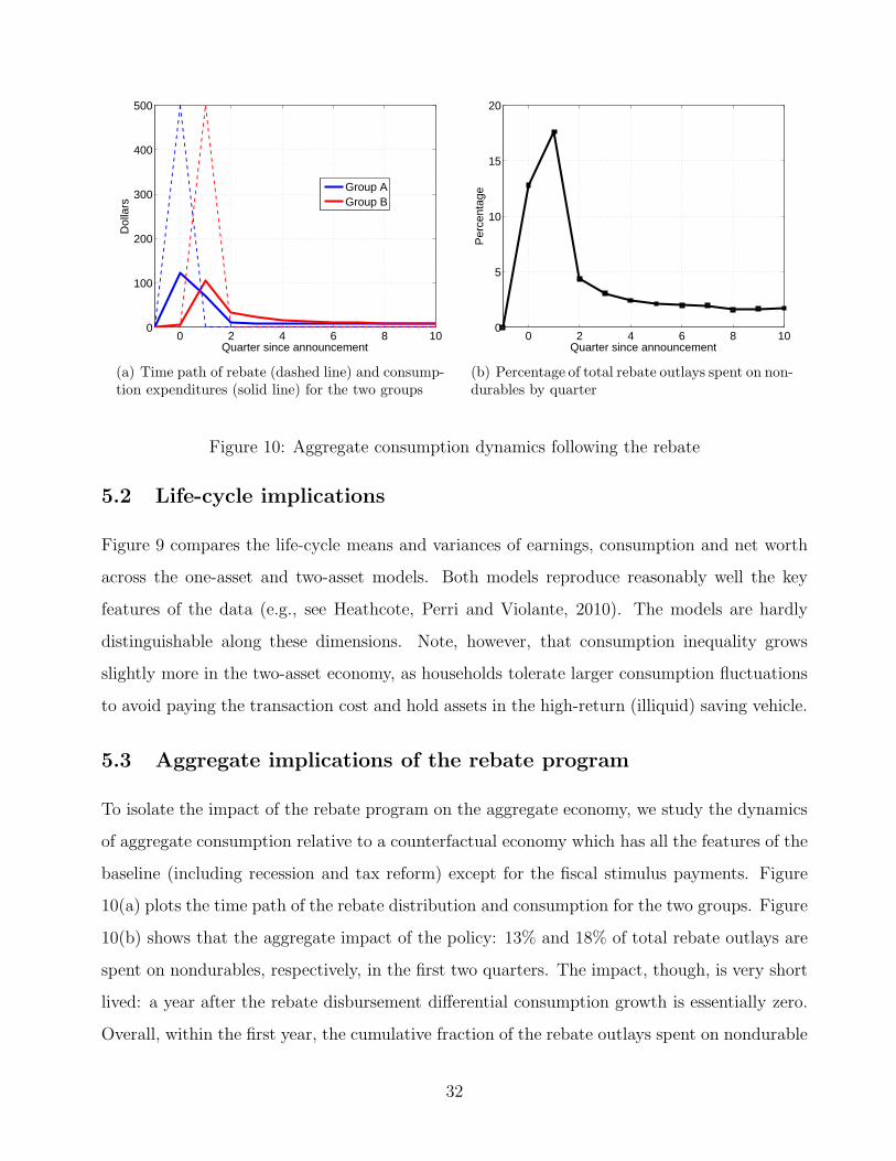
0 2 4 6 8 100

100

200

300

400

500

Quarter since announcement

Dol

lars

Group AGroup B

(a) Time path of rebate (dashed line) and consump-tion expenditures (solid line) for the two groups

0 2 4 6 8 100

5

10

15

20

Quarter since announcement

Per

cent

age

(b) Percentage of total rebate outlays spent on non-durables by quarter

Figure 10: Aggregate consumption dynamics following the rebate

5.2 Life-cycle implications

Figure 9 compares the life-cycle means and variances of earnings, consumption and net worth

across the one-asset and two-asset models. Both models reproduce reasonably well the key

features of the data (e.g., see Heathcote, Perri and Violante, 2010). The models are hardly

distinguishable along these dimensions. Note, however, that consumption inequality grows

slightly more in the two-asset economy, as households tolerate larger consumption fluctuations

to avoid paying the transaction cost and hold assets in the high-return (illiquid) saving vehicle.

5.3 Aggregate implications of the rebate program

To isolate the impact of the rebate program on the aggregate economy, we study the dynamics

of aggregate consumption relative to a counterfactual economy which has all the features of the

baseline (including recession and tax reform) except for the fiscal stimulus payments. Figure

10(a) plots the time path of the rebate distribution and consumption for the two groups. Figure

10(b) shows that the aggregate impact of the policy: 13% and 18% of total rebate outlays are

spent on nondurables, respectively, in the first two quarters. The impact, though, is very short

lived: a year after the rebate disbursement differential consumption growth is essentially zero.

Overall, within the first year, the cumulative fraction of the rebate outlays spent on nondurable

32

consumption is around 40%.

Since, in our model, we know the counterfactual path of aggregate consumption in the

absence of the rebate (but in the presence of the tax reform and recession), it is possible to

express the impact of the rebate as a percentage increase in aggregate consumption. We find

it to be 0.62% and 0.85% in the first two quarters, respectively. The cumulative increase in

aggregate consumption over the first year is 1.8%.

These calculations highlight two benefits of having a structural model that is consistent

with the micro evidence. First, because the tax reform and the recession affect consumption

even in the absence of the rebate, it is incorrect to measure consumption growth relative to a

baseline of consumption in the period before the rebate announcement. Rather, the full path

of counterfactual consumption should be taken into account. Second, to calculate the total

portion of the rebate that is spent, it is incorrect to multiply the rebate coefficient by the total

size of the rebate (as a fraction of aggregate consumption), as done for example by the CBO

(2009). The reason is that, as explained, the rebate coefficient β2 is not the MPC out of the

rebate, but the difference between the MPC for those who receive the check and that of the

rest of the population.

6 Robustness

In this Section, we discuss the robustness of our findings with respect to the timing of arrival of

the news, the specific process for individual earnings, the specific form of the transaction cost,

and the availability of consumer credit.

Arrival of news In Figure 11(a), we report the consumption response to the tax rebate

under alternative assumptions about when the news of the rebate enters households’ information

sets. When the rebate is a surprise for everyone, the rebate coefficient increases by around 5

percentage points on average. When it is anticipated by every household (the news arrives one

quarter ahead for the first group and two quarters ahead for the second group), the estimated

rebate coefficient drops by a similar amount. However, it still remains of a sizeable magnitude,

between 17% and 25% in the $500-$1,000 range for κ. The reason is that liquidity constrained

households are those driving the results and, for such households, learning that they will receive

33

0 500 1000 1500 2000 2500 30000

5

10

15

20

25

30

35

40

Reb

ate

Coe

ffici

ent (

%)

Fixed Cost ($)

Surprise for early recipients onlySurprise for nooneSurprise for all

(a) Rebate coefficients under alternative assump-tions on timing of the arrival of news

0 500 1000 1500 2000 2500 30000

5

10

15

20

25

30

35

40

Reb

ate

Coe

ffici

ent (

%)

Fixed Cost ($)

Permanent shocks modelHeterogeneous profiles model

(b) Rebate coefficients under alternative modelsfor earnings heterogeneity

Figure 11: Robustness analysis with respect to arrival of news and earnings heterogeneity

some income in the near future has little or no impact on their current consumption.41

Earnings heterogeneity In our baseline calibration we took the view that the increase

in earnings dispersion over the life-cycle is the result of the accumulation of highly persis-

tent idiosyncratic shocks. An alternative view, also quite common in the literature (Guvenen,

2009), is that it is the result of heterogeneity in deterministic idiosyncratic earnings profiles.

We re-estimated the parameters of our log household earnings process omitting the unit root

component zit and reinstating the household-specific slope ψi by matching the same set of

cross-sectional moments described in Section 4. The discount factor β is always set to match

median illiquid wealth, as in the baseline. Figure 11(b) compares the rebate coefficients in the

baseline model (without tax reform and recession). The implications of these two models are

very similar, but the heterogenous earnings profile model seems capable of generating slightly

larger rebate coefficients for a wide range of κ.

Transaction cost In the benchmark model, the fixed cost κ is the same across households.

Here we explored two alternative forms of transaction cost: proportional to individual earnings

(i.e., entering the budget constraint as −κyij), and in terms of utility (i.e., entering period

41When the rebate is anticipated by all households, even though the measured rebate coefficient is smaller, theaggregate cumulative effect on consumption is very similar to the baseline specification. This result reinforcesthe view that one should be cautious in using the value of the estimated rebate coefficient to draw inference onaggregate implications for consumption, as we argued in Section 5.3.

34

0 5 10 15 20 250

5

10

15

20

25

30

35

40

Cost (% of quarterly value)

Reb

ate

Coe

ffici

ent (

%)

Cost proportional to consumption

Cost proportional to earnings

(a) Rebate coefficients under alternative models for thetransaction cost

0 500 1000 1500 2000 2500 30000

5

10

15

20

25

30

35

40

45

Reb

ate

Coe

ffici

ent (

%)

Fixed Cost ($)

Low Rate: wedge = 0.05High Rate: wedge = 0.30

(b) Rebate coefficients under alternative borrow-ing rates. The reported wedge is relative to thereturn on the liquid asset

Figure 12: Robustness analysis with respect to credit and the form of the transaction cost

utility as log(cij) − κ. Given the log specification, the latter specification corresponds to a

cost proportional to individual consumption. The key difference with the baseline is that the

cost is not lump sum, but is larger for high income (or consumption) households. Figure

12(a) reports the rebate coefficients for these two models. Transaction costs of around 6% of

quarterly earnings or consumption yield values for the rebate coefficient around 25%, as in the

benchmark. For the median household whose annual earnings are $41,000 (see Table 2), this

cost corresponds to roughly $600.

Consumer credit A natural conjecture is that the rebate coefficient would be significantly

reduced by the existence of credit, if households that are paid the rebate later find it worthwhile

to borrow in anticipation of the fiscal stimulus payment. Figure 12(b) shows that in the model

this conjecture turns out to be correct only for an intermediate range on borrowing rates.42 For

high enough rates (e.g., “expensive” borrowing through credit cards), borrowing is too costly

and since households are not too impatient they are better off waiting for the check next quarter

than pre-empting consumption at the cost of large interest payments. For low enough rates

(e.g., “cheap” borrowing through home equity loans), there is an arbitrage opportunity in the

42In all the experiments of Figure 12(b), we have set the individual borrowing limit equal to their currentquarterly earnings, but the results are robust to changes in this parameter.

35

model: most households find it optimal to borrow up to the limit and save into the high-return

illiquid account.43 As a result, households tend to bunch at two kinks: zero and m. Since even

more households in this version of the model are at a kink, rebate coefficients are larger than

in the baseline (compare the top line of Figure 12(b) with the top line of Figure 6(a)). This

parameterization is instructive because it clearly illustrates that the addition of credit to the

model does not necessarily dampen rebate coefficients. Finally, as explained, for intermediate

interest rates the conjecture goes through and rebate coefficients drop substantially – even

though the amplification relative to the one asset model remains strong. Recall that in these

experiments we allow every household to access credit and they can do so at zero transaction

cost. Under costly access to credit, the results would be closer to our benchmark model.

7 Concluding remarks

The objective of this paper was to demonstrate how, by integrating the Baumol-Tobin model

with the standard incomplete-markets life-cycle framework, one can provide a theoretical foun-

dation, and a quantitative validation, for the observation that the MPC out of anticipated

temporary income changes is large – an empirical finding that is substantiated by robust quasi-

experimental evidence. Going forward, we plan to expand our analysis in several directions.

In using public funds to stimulate consumption, policy makers face a broad array of options,

of which across-the-board tax rebates are only one specific example. A key benefit of having

a fully structural model is that one can investigate the counterfactual welfare and aggregate

effects of alternative policies. Among the policies that we plan to study are more targeted tax

rebates and temporary reductions in consumption taxes, as was recently implemented in the

UK (see Blundell (2009)).

The model can be used to address the 2008 episode of fiscal stimulus payments. Under the

Economic Stimulus Act of 2008, households received on average nearly $1,000. PJSM (2011)

and Broda and Parker (2011) estimate rebate coefficients for nondurable expenditures between

half and 2/3 of the size of the 2001 estimates. The 2008 episode differs from the 2001 episode

43According to Greenspan and Kennedy (2008), 2/3 of the net proceeds of home equity loans are used forhome improvements and purchase of durables.

36

in three ways. First, its magnitude is roughly twice as large. Second, it is not part of any

broader tax reform. Third, eligibility phases out quickly starting at $75,000 of gross individual

income. Qualitatively, the lack of a tax reform and the larger rebate size suggest that the

model would generate a somewhat lower response in 2008, while the phasing out would induce

a higher response as more of the hand-to-mouth households are among the low-income ones

(although, as discussed in Section 5.1, we expect this effect to be weak). Moreover, the 2008

recession was much deeper than its 2001 counterpart: as explained in Section 5.1, it is a priori

unclear whether a deeper recession is associated with a higher or lower consumption response.

Overall, only a full quantitative analysis that contains all of these ingredients can shed light on

what accounted for the smaller impact on consumption of the 2008 stimulus program.

In calibrating our model, we have included the consumption flow of large durables (notably,

housing and cars) as part of the return. Modeling durables explicitly (with a consumption

flow proportional to the stock in the period utility function) would not affect the response of

nondurable consumption to the rebate, as long as utility is separable in the two consumption

goods. However, such an extension could be useful to study the aggregate implications of the

policy for consumption and output in more detail. Unsurprisingly, as documented by JPS

(2006) and PSJM (2011), when durable goods are included among expenditures, the response

of household consumption to the rebate almost doubles.44

Given the high-frequency OLG structure, solving a stochastic version of our model in general

equilibrium (i.e., with asset returns determined endogenously and aggregate shocks) is not

numerically feasible (see Krueger and Kubler, 2004). To make progress in these directions, one

could develop an infinite-horizon version of our economy (possibly with households transiting

randomly between work and retirement phases). To close the model, one would interpret the

illiquid asset a as productive capital with a return equal to its marginal product, whereas the

return on the liquid asset m could be pinned down by monetary policy (as in Ragot, 2011).

In this set up, one could also endow agents with rational beliefs over the probability that the

government will make fiscal stimulus payments during a recession, as in Heathcote (2005).

44See Guerrieri and Lorenzoni (2011) for a recent example of an incomplete-markets model with durable andnondurable consumption. As they emphasize, a crucial parameter affecting households’ response to an incomeshock is the degree of liquidity of durable goods.

37

References

Aiyagari, S. (1994): “Uninsured Idiosyncratic Risk and Aggregate Saving,” The Quarterly Journal

of Economics, 109(3), 659–684.

Aiyagari, S., and M. Gertler (1991): “Asset returns with transactions costs and uninsured

individual risk,” Journal of Monetary Economics, 27(3), 311–331.

Alvarez, F., A. Atkeson, and P. Kehoe (2002): “Money, interest rates, and exchange rates with

endogenously segmented markets,” Journal of Political Economy, 110(1), 73–112.

Angeletos, G., D. Laibson, A. Repetto, J. Tobacman, and S. Weinberg (2001): “The hyper-

bolic consumption model: Calibration, simulation, and empirical evaluation,” Journal of Economic

Perspectives, 15(3), 47–68.

Bai, J. (2005): “Stationary Monetary Equilibrium in a Baumol-Tobin Exchange Economy: Theory

and Computation,” Mimeo.

Blundell, R. (2009): “Assessing the temporary VAT cut policy in the UK,” Fiscal Studies, 30(1),

31–38.

Broda, C., and J. Parker (2008): “Estimates of the Impact of the 2008 Economic Stimulus

Payments on Consumption Demand,” Mimeo.

Browning, M., and M. Collado (2001): “The response of expenditures to anticipated income

changes: panel data estimates,” American Economic Review, 91(3), 681–692.

Browning, M., and T. Crossley (2001): “The life-cycle model of consumption and saving,”

Journal of Economic Perspectives, 15(3), 3–22.

Campbell, J., and Z. Hercowitz (2009): “Liquidity Constraints of the Middle Class,” Chicago

Fed Working Paper 2009-20.

Campbell, J., and N. Mankiw (1989): “Consumption, income, and interest rates: reinterpreting

the time series evidence,” NBER Macroeconomics Annual, 4, 185–216.

Card, D., R. Chetty, and A. Weber (2007): “Cash-On-Hand and Competing Models of In-

tertemporal Behavior: New Evidence from the Labor Market*,” Quarterly Journal of Economics,

122(4), 1511–1560.

Carroll, C. D. (1992): “The Buffer-Stock Theory of Saving: Some Macroeconomic Evidence,”

Brookings Papers on Economic Activity, 1992, 61–156.

(1997): “Buffer-Stock Saving and the Life Cycle/Permanent Income Hypothesis,” Quarterly

Journal of Economics, 112(1), 1–55.

Carroll, C. D., and M. S. Kimball (1996): “On the Concavity of the Consumption Function,”

Econometrica, 64(4), 981–992.

Chatterjee, S., and D. Corbae (1992): “Endogenous market participation and the general equi-

librium value of money,” Journal of Political Economy, 100(3), 615–646.

38

Chetty, R. (2011): “Bounds on Elasticities with Optimization Frictions: A Synthesis of Micro and

Macro Evidence on Labor Supply,” NBER Working Paper, 15616.

Cochrane, J. (1989): “The sensitivity of tests of the intertemporal allocation of consumption to

near-rational alternatives,” The American Economic Review, 79(3), 319–337.

Congressional Budget Office (2009): “Did the 2008 Tax Rebates Stimulate Short-Term

Growth?,” Economic and Budget Issue Brief.

Council of Economic Advisors (2010): “The Economic Impact of the American Recovery and

Reinvestment Act (Third Quarterly Report),” Executive Office of the President.

Deaton, A. (1991): “Saving and Liquidity Constraints,” Econometrica, 59(5), 1221–1248.

Erosa, A., and G. Ventura (2002): “On inflation as a regressive consumption tax,” Journal of

Monetary Economics, 49(4), 761–795.

Favilukis, J., S. Ludvigson, and S. Van Nieuwerburgh (2011): “The Macroeconomic Effects

of Housing Wealth, Housing Finance, and Limited Risk-Sharing in General Equilibrium,” mimeo.

Foundation, T. (2011): “Property Taxes on Owner Occupied Housing 2004-2009 by State,”

http://www.taxfoundation.org/research/show/1913.html.

Frenkel, J., and B. Jovanovic (1980): “On transactions and precautionary demand for money,”

The Quarterly Journal of Economics, 95(1), 25–43.

(1981): “Optimal international reserves: a stochastic framework,” The Economic Journal,

91(362), 507–514.

Greenspan, A., and J. Kennedy (2008): “Sources and uses of equity extracted from homes,”

Oxford Review of Economic Policy, 24(1), 120.

Guerrieri, V., and G. Lorenzoni (2010): “Credit Crises, Precautionary Savings and the Liquidity

Trap,” Chicago-Booth Working Paper.

Guvenen, F. (2009): “An empirical investigation of labor income processes,” Review of Economic

Dynamics, 12(1), 58–79.

Hall, R. (2011): “The long slump,” Discussion paper, National Bureau of Economic Research.

Hamilton, D. (2008): “A Reexamination of Johnson, Parker, and Souleles 2001 Tax Rebate Esti-

mate,” mimeo.

Heathcote, J. (2005): “Fiscal policy with heterogeneous agents and incomplete markets,” Review

of Economic Studies, 72(1), 161–188.

Heathcote, J., F. Perri, and G. Violante (2010): “Unequal We Stand: An Empirical Analysis

of Economic Inequality in the United States 1967-2006,” Review of Economic Dynamics, 13(1),

15–51.

Heathcote, J., K. Storesletten, and G. Violante (2009): “Quantitative Macroeconomics with

Heterogeneous Households,” Annual Reviews in Economics, 1.

39

Hsieh, C. (2003): “Do Consumers React to Anticipated Income Changes? Evidence from the Alaska

Permanent Fund,” American Economic Review, 93(1), 397–405.

Huggett, M. (1996): “Wealth Distribution in Life-cycle Economies,” Journal of Monetary Eco-

nomics, 38(3), 469–494.

Huntley, J., and V. Michelangeli (2011): “Can Tax Rebates Stimulate Spending in a Life-Cycle

Model?,” mimeo, CBO.

Imrohoroglu, A., and E. Prescott (1991): “Seigniorage as a Tax: A Quantitative Evaluation,”

Journal of Money Credit and Banking, 23(3), 462–475.

Johnson, D., J. Parker, and N. Souleles (2006): “Household expenditure and the income tax

rebates of 2001,” The American Economic Review, 96(5), 1589–1610.

(2009): “The Response of Consumer Spending to Rebates During an Expansion: Evidence

from the 2003 Child Tax Credit,” mimeo.

Joint Center For Housing Studies (2011): “A New Decade of Growth for Remodeling: Improving

America’s Housing,” mimeo.

Jovanovic, B. (1982): “Inflation and welfare in the steady state,” The Journal of Political Economy,

90(3), 561.

Kaplan, G., and G. Violante (2010): “How Much Consumption Insurance Beyond Self-

Insurance?,” American Economic Journals: Macroeconomics, 2(4), 53–87.

Khan, A., and J. Thomas (2010): “Inflation and Interest Rates with Endogenous Market Segmen-

tation,” Mimeo.

Kiefer, D., R. Carroll, J. Holtzblatt, A. Lerman, J. McCubbin, D. Richardson, and

J. Tempalski (2002): “The Economic Growth and Tax Relief Reconciliation Act of 2001: Overview

and Assessment of Effects on Taxpayers,” National Tax Journal, 55(1), 89–118.

Krueger, D., and F. Kubler (2004): “Computing equilibrium in OLG models with stochastic

production,” Journal of Economic Dynamics and Control, 28(7), 1411–1436.

Krusell, P., and A. Smith, Jr (1998): “Income and wealth heterogeneity in the macroeconomy,”

Journal of Political Economy, 106(5), 867–896.

Laibson, D. (1998): “Life-cycle consumption and hyperbolic discount functions,” European Economic

Review, 42(3-5), 861–871.

Luo, Y. (2008): “Consumption dynamics under information processing constraints,” Review of Eco-

nomic Dynamics, 11(2), 366–385.

Lusardi, A., D. Schneider, and P. Tufano (2011): “Financially Fragile Households: Evidence

and Implications,” Brookings Papers on Economic Activity, Forthcoming.

Mankiw, N. (2000): “The savers-spenders theory of fiscal policy,” American Economic Review, 90(2),

120–125.

40

McDaniel, C. (2007): “Average Tax Rates on Consumption, Investment, Labor and Capital in the

OECD: 1950–2003,” Mimeo, Arizona State University.

Miller, M., and D. Orr (1966): “A Model of the Demand for Money by Firms,” The Quarterly

Journal of Economics, 80(3), 413.

Misra, K., and P. Surico (2011): “Heterogeneous Responses and Aggregate Impact of the 2001

Income Tax Rebates,” CEPR DP, 8306.

Oh, H., and R. Reis (2011): “Targeted Transfers and the Fiscal Response to the Great Recession,”

NBER Working Paper, 16775.

Papke, L., and J. Poterba (1995): “Survey evidence on employer match rates and employee saving

behavior in 401 (k) plans,” Economics Letters, 49(3), 313–317.

Parker, J., N. Souleles, D. Johnson, and R. McClelland (2011): “Consumer Spending and

the Economic Stimulus Payments of 2008,” NBER Working Paper, 16684.

Ragot, X. (2011): “The case for a financial approach to money demand,” mimeo.

Reis, R. (2006): “Inattentive consumers,” Journal of Monetary Economics, 53(8), 1761–1800.

Rı́os-Rull, J. (1995): “Models with Heterogeneous Agents,” in Frontiers of Business Cycles Re-

search, ed. by T. F. Cooley, pp. 98–125. Princeton University Press.

Romer, D. (1986): “A simple general equilibrium version of the Baumol-Tobin model,” The Quarterly

Journal of Economics, 101(4), 663–685.

Shapiro, M., and J. Slemrod (2003a): “Consumer response to tax rebates,” American Economic

Review, 93(1), 381–396.

(2003b): “Did the 2001 Tax Rebate Stimulate Spending? Evidence from Taxpayer Surveys,”

Tax Policy and the Economy, 17, 83–109.

(2009): “Did the 2008 tax rebates stimulate spending?,” American Economic Review, 99(2),

374–379.

Souleles, N. (1999): “The response of household consumption to income tax refunds,” The American

Economic Review, 89(4), 947–958.

Telyukova, I. (2011): “Household Need for Liquidity and the Credit Card Debt Puzzle,” mimeo.

Thaler, R. (1990): “Anomalies: Saving, fungibility, and mental accounts,” The Journal of Economic

Perspectives, 4(1), 193–205.

41