Elise Koeniguer

Pol SAR App - Urban

Application of polarimetry to urban areas

Contact: elise.koeniguer@onera.fr ONERA Chemin de la Hunière et des Joncherettes BP 80100 FR-91123 PALAISEAU CEDEX

Outline

• Introduction: Urban applications

• Polarimetry: specificity of the urban context

• Applications

– Classification

– 3D

– subsidence

INTRODUCTION

Application of polarimetry to urban areas

Urban applications

• The world's population is rapidly increasing, especially in urban regions to which many rural inhabitants are migrating

• Results in the need for a efficient method of monitoring cities both in developing and developed countries

• Present monitoring techniques are inefficient and unable to maintain up-to date information

• Demand for settlement detection, urban classification and population estimation.

source: Population Division, UN: World Population Prospects

Motivation (1/2)

• Urban environments represent one of the most dynamic regions on earth. Due to these rapid changes, up-to-date spatial information is requisite for the effective management and mitigation of the effects of built-up dynamics.

• Alternative methods as air photo interpretation, national census and related statistics: time consuming, and expensive methods.

• Recent improvement in ground resolution in satellite remote sensing

• Radar benefits: irrespective of the light and weather conditions of the area being imaged.

Showcases on Urban in POLSAR App

Product Authors (Institution)

Detection of built-up areas Elise Koeniguer, Nicolas Trouvé (Onera)

Urban classification Y. Yamaguchi (Niigata University)

3D rendering by POLINSAR Elise Koeniguer, Nicolas Trouvé (Onera)

3D by tomography Yue Huang, Laurent Ferro-Famil (IETR Rennes)

Subsidence: ground deformation estimation Victor D. Navarro-Sanchez, Juan M. Lopez-Sanchez (University of Alicante)

Differential SAR interferometry Dani Monells, Rubén Iglesias, Xavier Fàbregas, Jordi Mallorquí, Albert Aguasca, Carlos López-Martínez (University of Catalunya)

APPLICATIONS

POLARIMETRY IN URBAN Application of polarimetry to urban areas

Main mechanisms

Lack of azimuthal symmetry

Orientation angle

Understanding the HV polarization over urban

main classical decompositions

The main mechanisms

layover roof shadow ground Ground

a b

c d

a

e

a a+c+d b d e a

θ

• Mixture of single mechanisms First case: h/tan θ > L

h

L

The main mechanisms

• Mixture of single mechanisms First case: h/tan θ < L

layover roof shadow ground Ground

a b

c d

a

e

a a+c+d a+c d e a

θ

The lack of azimuthal symmetry

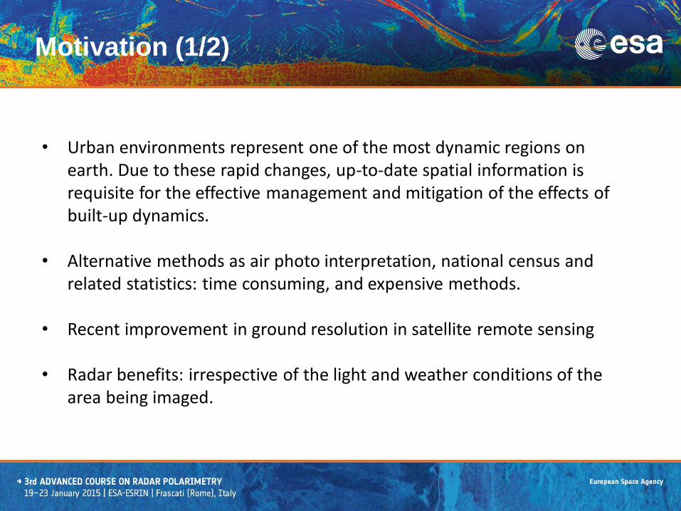
Example over Pi-SAR data

The orientation angle Induced either by: - tilted roof - dihedral effects non aligned with the azimuth

Azimuth line

Tilted roof Vertical wall

Vertical wall

φ

φ

α

Polarization orientation angle shifts computed from the polarimetric SAR data

Fully polarimetric image of a built-up housing area

Street pattern. Areas surrounded by the same colored lines possess similar alignment

Orientation angle of PiSAR L-band

(Sendaï)

Examples of POA over San Francisco images

-40

-30

-20

-10

0

10

20

30

40

X-band TerraSAR-X L-band ALOS-PALSAR

Noise level linked to the frequency bandwidth X-band: very noisy over vegetation and ocean L-band: very flat over ocean, noisy over vegetation

Use of the different polarimetric decompositions

• Coherent decompositions • Pauli

• Krogager

• Cameron

• Touzi criterion

• Incoherent decomposition • Based on eigenspace: Huynen, Barnes and Holm, Cloude Pottier, Holm

• « physical decomposition »: Freeman Durden, Yamaguchi, Van Zyl, Neumann

• Multiplicative decomposition: Lu and Chipman

APPLICATIONS

Application of polarimetry to urban areas

Classification

3D rendering

Subsidence

CLASSIFICATION

Application of polarimetry to urban areas

Based on polarimetric parameters Built-up detection using POLINSAR

Algorithms using POA and break of symetry

• Use of previous remarks

Results: classification

Yamaguchi versus Freeman Durden

• Yamaguchi better reduces the volume component

• But still fails to identify the 45° tilted block (SOMA district)

Yamaguchi and derived decompositions

• 3-component decomposition – Incoherent decomposition

– Surface, double, volume

T=Tsurf+Tdouble+Tvolume

• 4-component decomposition – 3-component + helix

– Volume scattering is modified

T=Tsurf+Tdouble+T’volume+Thelix

• 4-component decomposition with deorientation, 4-component applied to skew-oriented buildings

22

Intensity

Seems to be an interesting parameters to discriminate deterministic targets!

Use of interferometric coherence

Correlation After sub pixellic coregistration

Results: built-up detection

San Francisco

TerraSAR-X

0 0.2 0.4 0.6 0.8 10.2

0.3

0.4

0.5

0.6

0.7

0.8

0.9

1

PFA

PD

1MC optimal coherence

2MC optimal coherence

dual pol optimal coherence

coherence HV

coherence HH+VV

coherence HH-VV

0 0.2 0.4 0.6 0.8 10

0.2

0.4

0.6

0.8

1

PFA

PD

<|HV|2>

<|HH-VV|2>

<|HH+VV|2>

HV coherence

HH-VV coherence

HH+VV coherence

3D

Application of polarimetry to urban areas

POLINSAR POLTOMSAR

Comparison single pass – multi pass at X-band

25

Information avalaible only on buildings

Hue : interferometric phase Intensity : span: Saturation : coherence level

Interferometric phase at X-band over Toulouse: singla pass

Interferometric phase at X-band over San Francisco : repeat pass

Height estimation based on coherence shapes

A

B

-1 -0.5 0 0.5 1-1

-0.5

0

0.5

1

0.2

0.4

0.6

0.8

1

30

210

60

240

90

270

120

300

150

330

180 0

Re

Im

-1 -0.5 0 0.5 1-1

-0.5

0

0.5

1

0.2

0.4

0.6

0.8

1

30

210

60

240

90

270

120

300

150

330

180 0

Re

Im

-1 -0.5 0 0.5 1-1

-0.5

0

0.5

1

0.2

0.4

0.6

0.8

1

30

210

60

240

90

270

120

300

150

330

180 0

Re

Im

Towards statistical models to predict coherence shapes

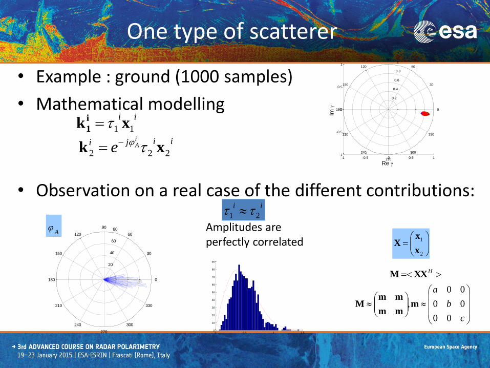
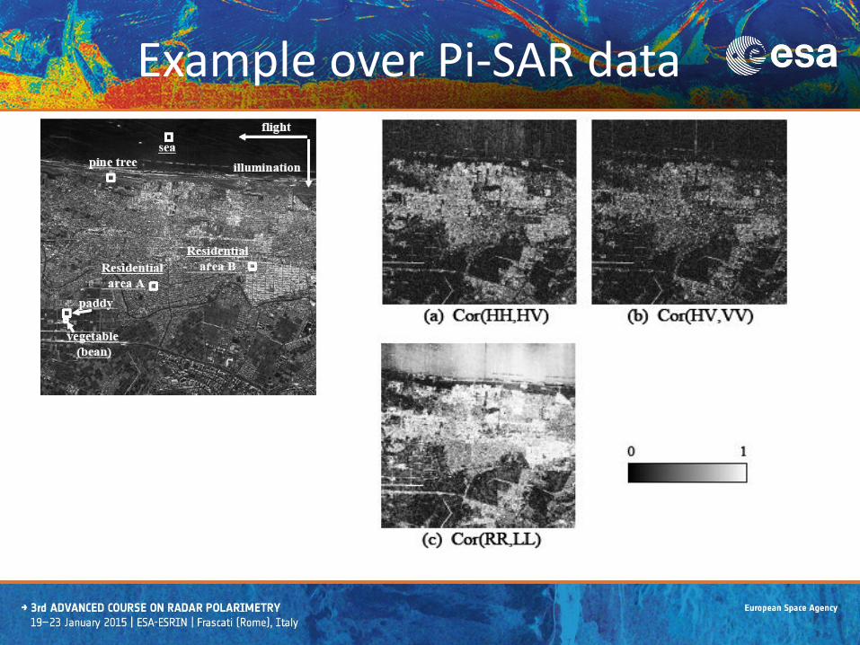
One type of scatterer

• Example : ground (1000 samples)

• Mathematical modelling

• Observation on a real case of the different contributions:

ii

11 xki

1 iiji

iAe 222 xk

-1 -0.5 0 0.5 1

-1

-0.5

0

0.5

1

0.2

0.4

0.6

0.8

1

30

210

60

240

90

270

120

300

150

330

180 0

Re

Im

20

40

60

80

30

210

60

240

90

270

120

300

150

330

180 0

A

ii

21

Amplitudes are perfectly correlated

0 0.5 1 1.50

10

20

30

40

50

60

70

80

90

2

1

x

xX

HXXM

c

b

a

00

00

00

,mmm

mmM

• With no correlation between polarimetric vectors (1)

• With two equal polarimetric vectors (maximum interferometric correlation) (2)

• With a covariance matrix for and non zero extradiagonal elements (3)

Statistical hypothesis Associated coherence Shape

-1 -0.5 0 0.5 1-1

-0.5

0

0.5

1

0.2

0.4

0.6

0.8

1

30

210

60

240

90

270

120

300

150

330

180 0

Re

Im

Correlation between polarimetric pair

-1 -0.5 0 0.5 1-1

-0.5

0

0.5

1

0.2

0.4

0.6

0.8

1

30

210

60

240

90

270

120

300

150

330

180 0

Re

Im

-1 -0.5 0 0.5 1-1

-0.5

0

0.5

1

0.2

0.4

0.6

0.8

1

30

210

60

240

90

270

120

300

150

330

180 0

Re

Im

ii

21 xx

021 Hji

xx

021 Hji

xx

2

1

x

xX

(1) (2)

(3)

021 Hji

xx

021 Hji

xxii

21 xx

Modelling of a 2 bright point cell

• Mathematical modelling

• Mixture of two different polarimetric statistics on points A and B:

i

B

i

Ai

B

i

A

1

111 ,

xxk

i

1

i

B

i

A

j

ji

B

i

A iB

iA

e

e

2

2222

0

0,

xxki

11 cS22 cDS

A

A

A

2

1

x

xX

H

AAA XXM H

BBB XXM

B

B

B

2

1

x

xX

iB

i

A 11 ,xxS1

iB

i

A 22 ,xxS2

Point A Point B

Estimation of coherence on real data

• Ground segments and building segments

-1 -0.5 0 0.5 1-1

-0.5

0

0.5

1

0.2

0.4

0.6

0.8

1

30

210

60

240

90

270

120

300

150

330

180 0

Re

Im

-1 -0.5 0 0.5 1-1

-0.5

0

0.5

1

0.2

0.4

0.6

0.8

1

30

210

60

240

90

270

120

300

150

330

180 0

estimation classique

Re

Im

-1 -0.5 0 0.5 1-1

-0.5

0

0.5

1

0.2

0.4

0.6

0.8

1

30

210

60

240

90

270

120

300

150

330

180 0

Re

Im

-1 -0.5 0 0.5 1-1

-0.5

0

0.5

1

0.2

0.4

0.6

0.8

1

30

210

60

240

90

270

120

300

150

330

180 0

Re

Im

Building segments with polarimetric diversity

Bare soil segments

Building segments without internal polarimetric diversity

Height estimation

Segmentation et estimation 3D

données Google 3D INSA/Université

Root mean squared error

Results: 3D rendering

Polarization use

Ground truth height – estimated height (m)

RMSE (m)

HH+VV 2,57 3,89

HH-VV 2,76 4,60

HV 2,23 3,79

Dual pol 1,20 3,76

Full pol 1,20 2,87

Tomography

• MB Insar Approach : heights, layover sources

• Polarimetry + InSAR :

Example of tomograms

• E-SAR L-band Pauli color-coded urban scene

Pseudotomographic slices of the optimal MUSIC scattering mechanisms

Refined characterization of building height and scattering mechanisms

Results: tomography

3-D reconstruction: LiDAR (left) and FP-NSF estimator (right).

SUBSIDENCE

Application of polarimetry to urban areas

subsidence

• Why subsidence in urban areas ? may be caused by factors including

• groundwater extraction

• load of constructions

• natural consolidation of alluvium soil

• geotectonic subsidence

Monitoring of land subsidence

is required for – groundwater extraction regulation,

– effective flood control and seawater intrusion,

– conservation of environment

– construction of infrastructure, and spatial development planning in general.

Bologne

Ast

riu

m G

EO-I

nfo

rma

tio

n S

ervi

ces

Contribution of POLSAR to PSI

• Persistent Scatteter Interferometry yields ground deformation values, along time, for a set of pixels selected (PSC: persistent scatterer candidates) from the images

• Key point: A good density and spatial distribution of the PSC is required for:

– InSAR processing (e.g. phase unwrapping)

– Model adjustment (arcs and integration)

– Atmospheric phase screen (APS) consistent estimation/removal

• Selection of PSC: pixels whose phase is stable (not noisy) in time

– Problem: we cannot trust directly in the measured phases

– Selection criteria:

• Low amplitude dispersion (SLC images)

• High average interferometric coherence (multi-looked interferograms)

Example in Murcia (Spain), with 45 TerraSAR-X images HHVV

Coherence: 60%

Amplitude: 170%

Increase in number of

pixels over single-pol:

Contribution of POLSAR to PSI

1st contribution of polarimetry to PSI: increase the number of PSC by optimising the quality criteria

Results: ground deformation

Number of Reliable Pixels Selected (Coherence Stability)a

Method Number of pixels

hh 6431 (3.3%)

hv 5026 (2.6%)

vv 5014 (2.6%)

Best 11931 (6.1%)

SOM 13894 (7.1%)

ESM 17281 (8.9%)

(a) HH (b) Best (c) SOM (d) ESM optimization methods.

CONCLUSIONS Application of polarimetry to urban areas

Conclusions

Classification

• X-band: very recent development. In this context, polarimetry only seems to become less effective for discriminating built-up areas. Essential contribution of polarimetry in the detection of built-up areas is the optimization of the PolInSAR coherence. It is used to discriminate targets based on their speed of temporal decorrelation.

• As regards the contribution of HV versus dual mode pol HH / VV, the situation is less clear, essentially due to the poor SNR in the HV channel of TerraSAR-X data.

• Still at X-band, the correlation coefficient in the circular polarization basis contains useful information on objects. It can be used for classification, derivation of surface slope, polarization orientation angle, among others. Not applicable to single/dual polarimetric data sets.

Conclusions

• Polarimetry improves the precision obtained on the height estimates of a factor of two. The mean squared error has been reduced also.

• Full polarimetry improves the RMSE versus dual polarimetry

• Among all single polarizations, the HV gives the best results

• Errors and estimation difficulties are mainly: • Bad choice of the population of pixels belonging to the roof. • Sources of polarimetric decorrelation of interferometric noise.

3D rendering (POLINSAR – Tomography)

Conclusions

Subsidence

• The polarimetric optimization methods demonstrate its capability to enhance the quality of DInSAR and PSI results:

• higher density of pixels compared with the single polarization case. • quality of the interferometric phase is also improved, leading to more precise

deformation maps

• First experiments with full-pol data show a more significant improvement than dual-pol, increasing the density of selected pixels up to twice with respect to dual-pol optimised data, and more than four times with respect to single-pol.

• Including the HV channel in the processing adds a great deal of information, given the important cross-polar response coming from tilted dihedrals in urban areas (oriented buildings).