Embed Size (px)
DESCRIPTION
Tutorial on Basics of SAR Polarimetry Based on POLARIMETRIC RADAR IMAGINGFrom Basics to ApplicationsBy - JONG-SEN LEE • ERIC POTTIER
Citation preview
Basic SAR Polarimetry 2013
1 Divyesh M. Varade ([email protected]) GI|CE|IITK
Basic SAR Polarimetry Fundamentals
Summary:
This report is developed for the partial fulfillment of the training program conducted during the
summer semester in the Center for Studies in Resource Engineering at the Indian Institute of
Technology Bombay. This report is meant to serve as a tutorial guide. In this tutorial the basics
concepts associated to Synthetic Aperture Radar are briefly discussed along with illustrations.
Title Basic SAR Polarimetry Domain Area Microwave Remote Sensing
Supervision Dr. Avik Bhattacharya
Report Version 1.1
Submission 18-Jul-13 Author Doktorand. MSc-Ing. Divyesh M. Varade
Editorial Board NERD, IITK Geoiformatics Dept. of Civil Engg. Indian Institute of Technology Kanpur C-303, Hall-7. 9651854411
Basic concepts of Synthetic Aperture Radar-SAR Polarimetry for beginners. Initial unedited first version.

Basic SAR Polarimetry 2013
2 Divyesh M. Varade ([email protected]) GI|CE|IITK
ACKNOWLEDGEMENT
I would like to hereby express my gratitude to all the people involved during this training program.
First of all, I would like to express my sincere thanks to Prof. G Venkataraman for supporting this
program and providing the financial support during this program. I would like also like to thank Dr.
Avik Bhattacharya for introducing me to the world of SAR Polarimetry. Without his guidance this
training program would not have been this successful. I truly appreciate his mode of conduct for the
instructions and his thoughtfulness to the simple minded. I would also take this opportunity to
thank my supervisor Prof. Onkar Dixit for believing in me and enthusiastically encouraging me to
take this training program.
Last but not least, I want to thank all my other superiors, peers, my colleagues and friends for
holding through with me. I am grateful for the numerous discussions I have had with them, that
have assisted in the thorough understanding of concepts involved on course this program.
Basic SAR Polarimetry 2013
3 Divyesh M. Varade ([email protected]) GI|CE|IITK
TABLE OF CONTENTS
1. Electromagnetism and Polarization ...................................................................................................... 5
1.1. Electromagnetism ................................................................................................................................................ 5
1.2. Wave Propagation ................................................................................................................................................ 6
1.3. Polarization ............................................................................................................................................................. 6
1.3.1. Linear (plane) polarization .................................................................................................................... 7
1.3.2. Circular polarization ................................................................................................................................. 8
1.3.3. Elliptical Polarization ................................................................................................................................ 8
1.4. Polarization Ellipse .............................................................................................................................................. 9
1.5. Deschamp’s Parameters (γ,δ) ....................................................................................................................... 11
1.5.1. Relation between (γ, δ) and (φ, τ) .......................................................................................................... 11
2. Jones Vector Formulation ....................................................................................................................... 13
2.1. Basic Formulation .............................................................................................................................................. 13
2.2. Generalization of Jones Vector ...................................................................................................................... 14
3. Stokes Parameters and Poincáre Sphere .......................................................................................... 16
3.1. Stokes Parameters ............................................................................................................................................. 16
3.1.1. Roll invariance of Stokes Parameters .............................................................................................. 17
3.2. Poincáre Sphere .................................................................................................................................................. 18
3.3. Representation of Poincáre Sphere with Complex polarization ratio .......................................... 20
4. Partially Polarized EM wave .................................................................................................................. 23
4.1. Coherency Matrix [J] ......................................................................................................................................... 24
4.2. Stokes vectors for partially polarized EM wave .................................................................................... 26
4.3. Degree of Polarization (DoP)......................................................................................................................... 26
4.4. Entropy (H), Anisotropy (Aw) and relation between DOP and H .................................................. 27
4.4.1. Entropy (H) & Anisotropy (Aw) ......................................................................................................... 27
4.4.2. Relation between DOP and H ............................................................................................................... 28
5. Change of Polarimetric Basis ................................................................................................................. 30
5.1. Special Unitary decomposition of E vector .............................................................................................. 30
5.1.1. Pauli Matrices ............................................................................................................................................. 30
5.2. Orthogonal polarization states and polarization basis ....................................................................... 31
5.3. Change of Polarimetric Basis ......................................................................................................................... 31
5.3.1. Cartesian to Elliptical Orthonormal basis ...................................................................................... 32
5.3.2. Cartesian to Circular basis .................................................................................................................... 32
6. Complex Polarization Ratio ................................................................................................................... 34
6.1.1. Complex Polarization Ratio in an arbitrary basis ............................................................................ 34
6.1.2. Complex polarization ratio in the linear basis {H V} ...................................................................... 35
6.1.3. Complex polarization ratio in the circular basis {L, R} .................................................................. 35
6.1.4. Complex polarization ratio in the linear basis {45° 135°} ............................................................ 35

Basic SAR Polarimetry 2013
4 Divyesh M. Varade ([email protected]) GI|CE|IITK
7. Radar Target Cross Section .................................................................................................................... 36
7.1. The Radar Equation (from Skolnik, 1981) ............................................................................................... 36
7.2. Radar Target Cross-Section [RCS] ............................................................................................................... 38
7.3. Distributed Targets ........................................................................................................................................... 39
8. Scattering Polarimetry ............................................................................................................................ 40
8.1. Radar Target Interaction ................................................................................................................................. 40
8.2. Scattering Matrix ................................................................................................................................................ 42
8.3. Reciprocity Theorem ........................................................................................................................................ 43
8.4. Scattering Theory ............................................................................................................................................... 43
8.5. Scattering Coordinate Frameworks (Lee and Pottier, 2009). .......................................................... 44
8.5.1. Coherent Jones Scattering Matrix [S] ............................................................................................... 45
8.5.2. Sinclair Matrix ............................................................................................................................................ 46
8.6. Scattering Target Vectors (Lee and Pottier, 2009)............................................................................... 47
8.6.1. Bistatic Case ................................................................................................................................................ 47
8.6.2. Monostatic Case......................................................................................................................................... 48
8.7. Coherency [T] and Covariance [C] Matrices (Lee and Pottier, 2009) ........................................... 49
8.7.1. Bistatic Case ................................................................................................................................................ 50
8.7.2. Monostatic Case......................................................................................................................................... 51
8.8. Mueller [M] and Kennaugh [K] matrices (Lee and Pottier, 2009) ................................................. 51
8.8.1. Bistatic Case ................................................................................................................................................ 52
8.8.2. Monostatic Case......................................................................................................................................... 54
9. Single look complex image an overview ............................................................................................ 56
9.1. Phase Correlation between real and imaginary components. ......................................................... 57
9.1.1. Forest Area .................................................................................................................................................. 58
9.1.2. Grassland...................................................................................................................................................... 58
9.1.3. Lake Area ..................................................................................................................................................... 59
9.1.4. Gilching Urban Area................................................................................................................................. 60
9.1.5. Wessling Urban Area ............................................................................................................................... 61
9.2. Statistical Comparison with Normal Distribution ................................................................................ 62
9.3. SLC Image Phase analysis ............................................................................................................................... 64
9.4. Basis Change ......................................................................................................................................................... 67
Appendix ................................................................................................................................................................ 71
A. Proof for Coherency Matrix being Hermitian ............................................................................................. 71
B. Positive Semi-definite Matrix ............................................................................................................................. 71
References ............................................................................................................................................................. 72
Basic SAR Polarimetry 2013
5 Divyesh M. Varade ([email protected]) GI|CE|IITK
1. Electromagnetism and Polarization
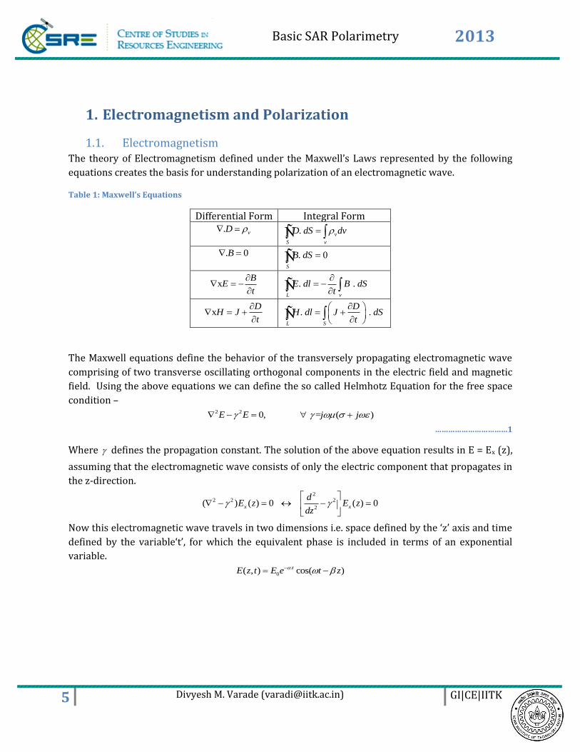
1.1. Electromagnetism The theory of Electromagnetism defined under the Maxwell’s Laws represented by the following
equations creates the basis for understanding polarization of an electromagnetic wave.
Table 1: Maxwell’s Equations
Differential Form Integral Form . vD . v
S v
D dS dv Ñ
. 0B . 0S
B dS Ñ
xB
Et
. .
L v
E dl B dSt
Ñ
xD
H Jt
. .
L S
DH dl J dS
t
Ñ
The Maxwell equations define the behavior of the transversely propagating electromagnetic wave
comprising of two transverse oscillating orthogonal components in the electric field and magnetic
field. Using the above equations we can define the so called Helmhotz Equation for the free space
condition – 2 2 0, = ( )E E j j
……………………………1
Where defines the propagation constant. The solution of the above equation results in E = Ex (z),
assuming that the electromagnetic wave consists of only the electric component that propagates in
the z-direction. 2
2 2 2
2( ) ( ) 0 ( ) 0x x
dE z E z
dz
Now this electromagnetic wave travels in two dimensions i.e. space defined by the ‘z’ axis and time
defined by the variable‘t’, for which the equivalent phase is included in terms of an exponential
variable.
0( , ) cos( )zE z t E e t z
Basic SAR Polarimetry 2013
6 Divyesh M. Varade ([email protected]) GI|CE|IITK
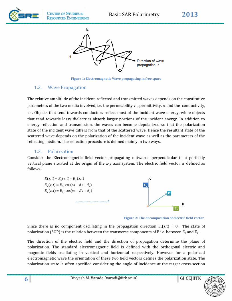
Figure 1: Electromagnetic Wave propagating in free space
1.2. Wave Propagation
The relative amplitude of the incident, reflected and transmitted waves depends on the constitutive
parameters of the two media involved, i.e. the permeabilityε, permittivity,μand the conductivity,
σ. Objects that tend towards conductors reflect most of the incident wave energy, while objects
that tend towards lossy dielectrics absorb larger portions of the incident energy. In addition to
energy reflection and transmission, the waves can become depolarized so that the polarization
state of the incident wave differs from that of the scattered wave. Hence the resultant state of the
scattered wave depends on the polarization of the incident wave as well as the parameters of the
reflecting medium. The reflection procedure is defined mainly in two ways.
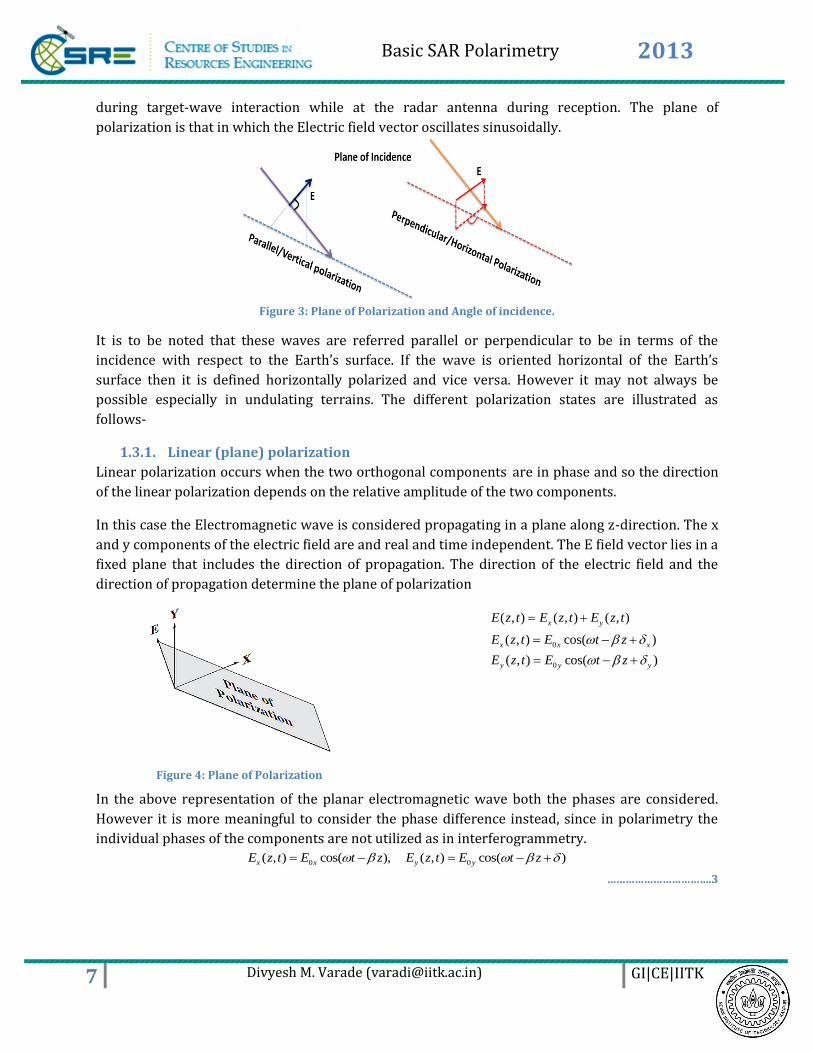
1.3. Polarization Consider the Electromagnetic field vector propagating outwards perpendicular to a perfectly
vertical plane situated at the origin of the x-y axis system. The electric field vector is defined as
follows-
0
0
( , ) ( , ) ( , )
( , ) cos( )
( , ) cos( )
x y
x x x
y y y
E z t E z t E z t
E z t E t z
E z t E t z
………………………………2
Figure 2: The decomposition of electric field vector
Since there is no component oscillating in the propagation direction Ez(z,t) = 0. The state of
polarization (SOP) is the relation between the transverse components of E i.e. between Ex and Ey.
The direction of the electric field and the direction of propagation determine the plane of
polarization. The standard electromagnetic field is defined with the orthogonal electric and
magnetic fields oscillating in vertical and horizontal respectively. However for a polarized
electromagnetic wave the orientation of these two field vectors defines the polarization state. The
polarization state is often specified considering the angle of incidence at the target cross-section
Basic SAR Polarimetry 2013
7 Divyesh M. Varade ([email protected]) GI|CE|IITK
during target-wave interaction while at the radar antenna during reception. The plane of
polarization is that in which the Electric field vector oscillates sinusoidally.
Figure 3: Plane of Polarization and Angle of incidence.
It is to be noted that these waves are referred parallel or perpendicular to be in terms of the
incidence with respect to the Earth’s surface. If the wave is oriented horizontal of the Earth’s
surface then it is defined horizontally polarized and vice versa. However it may not always be
possible especially in undulating terrains. The different polarization states are illustrated as
follows-
1.3.1. Linear (plane) polarization
Linear polarization occurs when the two orthogonal components are in phase and so the direction
of the linear polarization depends on the relative amplitude of the two components.
In this case the Electromagnetic wave is considered propagating in a plane along z-direction. The x
and y components of the electric field are and real and time independent. The E field vector lies in a
fixed plane that includes the direction of propagation. The direction of the electric field and the
direction of propagation determine the plane of polarization
Figure 4: Plane of Polarization
0
0
( , ) ( , ) ( , )
( , ) cos( )
( , ) cos( )
x y
x x x
y y y
E z t E z t E z t
E z t E t z
E z t E t z
In the above representation of the planar electromagnetic wave both the phases are considered.
However it is more meaningful to consider the phase difference instead, since in polarimetry the
individual phases of the components are not utilized as in interferogrammetry.
0 0( , ) cos( ), ( , ) cos( )x x y yE z t E t z E z t E t z
…………………………….3
Basic SAR Polarimetry 2013
8 Divyesh M. Varade ([email protected]) GI|CE|IITK
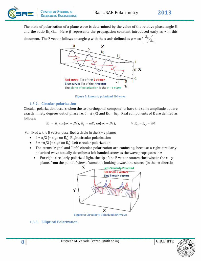
The state of polarization of a plane wave is determined by the value of the relative phase angle δ,
and the ratio E0y/E0x. Here β represents the propagation constant introduced early as γ in this
document. The E vector follows an angle φ with the x-axis defined as 1 0
0
tan y
x
E
E
Figure 5: Linearly polarized EM wave.
1.3.2. Circular polarization
Circular polarization occurs when the two orthogonal components have the same amplitude but are
exactly ninety degrees out of phase i.e. δ = ±π/2 and E0x = E0y. Real components of E are defined as
follows:
0 00 0 , , 0x yx yE E cos t z E E E E Esin t z m
For fixed z, the E vector describes a circle in the x − y plane:
δ = π/2 (− sign on Ey): Right circular polarization
δ = −π/2 (+ sign on Ey): Left circular polarization
The terms “right” and “left” circular polarization are confusing, because a right-circularly-
polarized wave actually describes a left-handed screw as the wave propagates in z
For right-circularly-polarized light, the tip of the E vector rotates clockwise in the x − y
plane, from the point of view of someone looking toward the source (in the −z directio
Figure 6: Circularly Polarized EM Wave.
1.3.3. Elliptical Polarization
Basic SAR Polarimetry 2013
9 Divyesh M. Varade ([email protected]) GI|CE|IITK
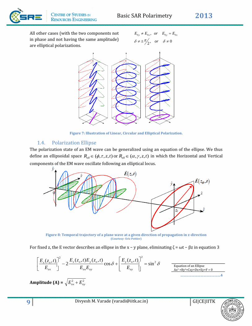
All other cases (with the two components not
in phase and not having the same amplitude)
are elliptical polarizations.
0 0 0 0,
, 02
y x y xE E or E E
or
Figure 7: Illustration of Linear, Circular and Elliptical Polarization.
1.4. Polarization Ellipse The polarization state of an EM wave can be generalized using an equation of the ellipse. We thus
define an ellipsoidal space ),,,(or ),,,( tzRtzR ellell in which the Horizontal and Vertical
components of the EM wave oscillate following an elliptical locus.
Figure 8: Temporal trajectory of a plane wave at a given direction of propagation in z-direction
(Courtesy- Eric Pottier)
For fixed z, the E vector describes an ellipse in the x − y plane, eliminating ζ = ωt − βz in equation 3
2
22
sin),(
cos),(),(
2),(
oy
oy
oyox
oyox
ox
ox
E
tzE
EE
tzEtzE
E
tzE
……………………………………4
Amplitude (A) = 22
oyox EE
Equation of an Ellipse Ax2 +By2+Cxy+Dx+Ey+F = 0
Basic SAR Polarimetry 2013
10 Divyesh M. Varade ([email protected]) GI|CE|IITK
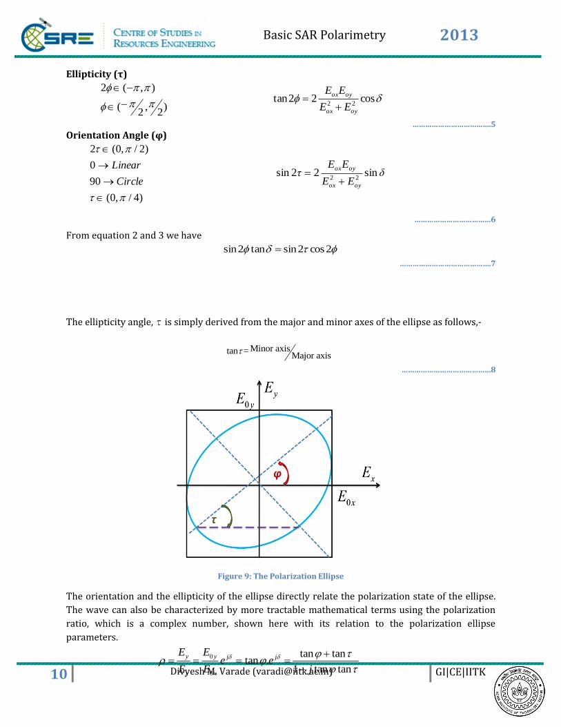
Ellipticity (τ)
)2
,2
(
),(2
cos22tan
22
oyox
oyox
EE
EE
……………………………….5
Orientation Angle (φ)
)4/,0(
90
0
)2/,0(2
Circle
Linear δ
EE
EEτ
oyox
oyoxsin22sin
22
………………………………6
From equation 2 and 3 we have
2cos2sintan2sin
…………………………………….7
The ellipticity angle,τis simply derived from the major and minor axes of the ellipse as follows,-
Minor axistan = Major axis
……………………………………8
Figure 9: The Polarization Ellipse
The orientation and the ellipticity of the ellipse directly relate the polarization state of the ellipse.
The wave can also be characterized by more tractable mathematical terms using the polarization
ratio, which is a complex number, shown here with its relation to the polarization ellipse
parameters.
0
0
tan tantan .
1 tan tan
y y j j
x x
E Ee e
E E j
Basic SAR Polarimetry 2013
11 Divyesh M. Varade ([email protected]) GI|CE|IITK
…………………………….9
For a circularly polarized wave, the EM wave is a sum of equal amplitude left-hand circular
polarized and right-hand circular polarized components. The polarization ratio is then defined as
1 1 1
1 1 1
l
r
E j p qq p j
E j p q
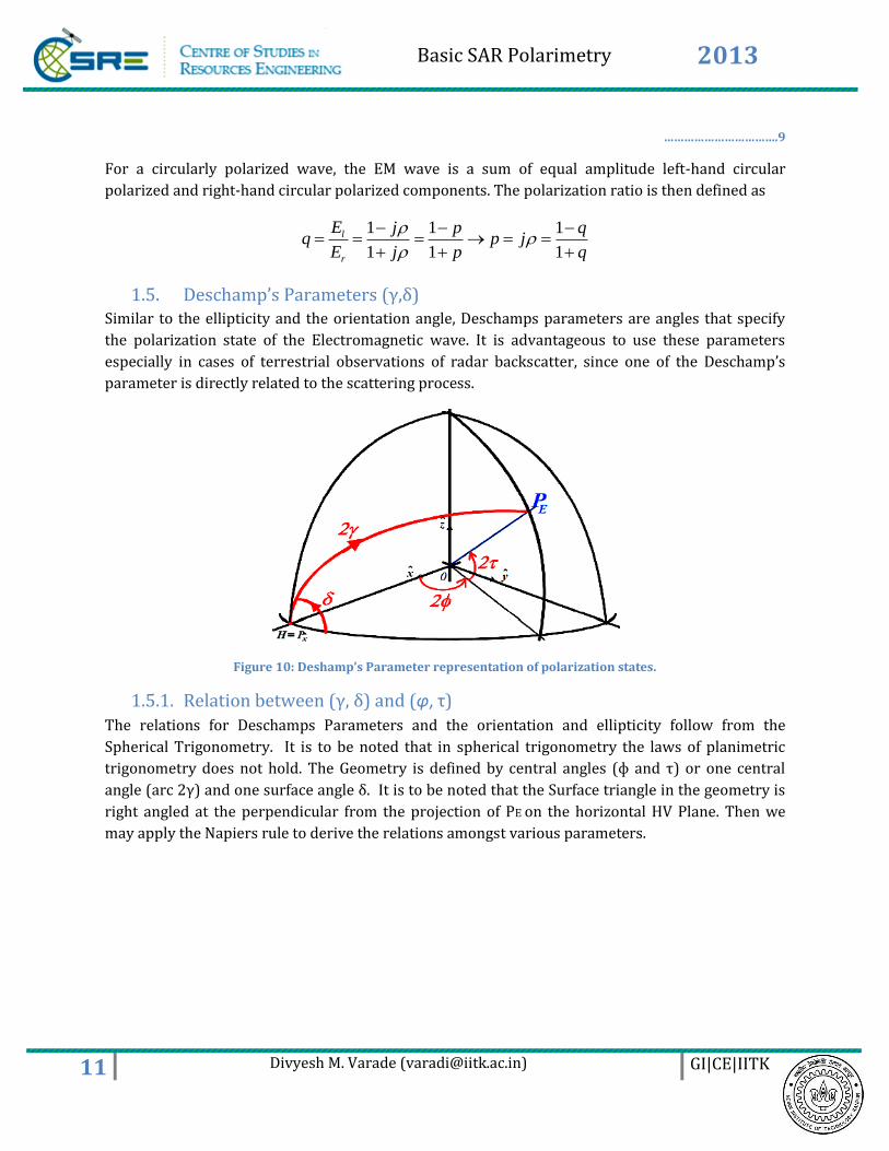
1.5. Deschamp’s Parameters (γ,δ) Similar to the ellipticity and the orientation angle, Deschamps parameters are angles that specify
the polarization state of the Electromagnetic wave. It is advantageous to use these parameters
especially in cases of terrestrial observations of radar backscatter, since one of the Deschamp’s
parameter is directly related to the scattering process.
Figure 10: Deshamp’s Parameter representation of polarization states.
1.5.1. Relation between (γ, δ) and (φ, τ)
The relations for Deschamps Parameters and the orientation and ellipticity follow from the
Spherical Trigonometry. It is to be noted that in spherical trigonometry the laws of planimetric
trigonometry does not hold. The Geometry is defined by central angles (ф and τ) or one central
angle (arc 2γ) and one surface angle δ. It is to be noted that the Surface triangle in the geometry is
right angled at the perpendicular from the projection of PE on the horizontal HV Plane. Then we
may apply the Napiers rule to derive the relations amongst various parameters.
Basic SAR Polarimetry 2013
12 Divyesh M. Varade ([email protected]) GI|CE|IITK
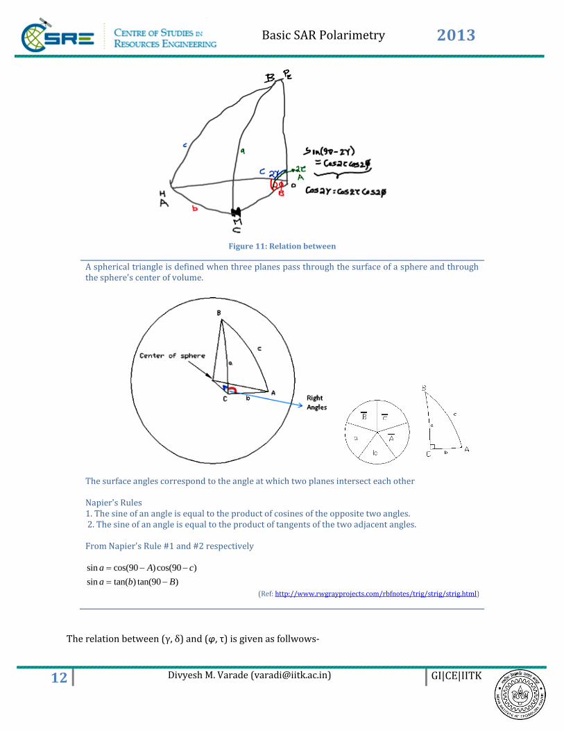
Figure 11: Relation between
A spherical triangle is defined when three planes pass through the surface of a sphere and through the sphere's center of volume.
The surface angles correspond to the angle at which two planes intersect each other Napier's Rules 1. The sine of an angle is equal to the product of cosines of the opposite two angles. 2. The sine of an angle is equal to the product of tangents of the two adjacent angles. From Napier's Rule #1 and #2 respectively sin cos(90 )cos(90 )
sin tan( ) tan(90 )
a A c
a b B
(Ref: http://www.rwgrayprojects.com/rbfnotes/trig/strig/strig.html)
The relation between (γ, δ) and (φ, τ) is given as follwows-
Basic SAR Polarimetry 2013
13 Divyesh M. Varade ([email protected]) GI|CE|IITK
cos 2 cos 2 cos 2
tan tan 2 cos 2ec
…………………………………..10
2. Jones Vector Formulation
2.1. Basic Formulation The Jones vector is introduced as a matrix representation of the polarization state of the electric
field. The Jones vector that represents a polarization state can be decomposed into any orthogonal
polarization basis. Jones Vector describes the planimetric representation of an electromagnetic
field to describe its polarization states as a point on the Poincáre sphere (section 3.2) using a
minimal two parameters.
For an EM wave we have two fields as from equation 3, which can be postulated in a matrix form:
yj
oy
xj
ox
yoy
xox
eE
eEE(z,t)=
)kzt(|E
)kzt(||EE(z,t)=
cos|
cos
………………………11
Equation (1) can also be formulated as follows:
)kzt(
oy
kz)t(
ox
oy
ox
eE(y,t)=E
eE(x,t)=E
)kzt(E(y,t)=E
kz)t(E(x,t)=E
cos
cos
eE(y,t)=E
E(x,t)=Ee
eE(y,t)=E
eE(x,t)=E
eE(y,t)=E
eE(x,t)=E
oy
ox
)(
oy
ox
)kzt(
oy
kz)t(
ox
cos
sin
ox x
j j
oy y
E(x,t)= E E =e e
E(y,t)= E e E = e
eeeeEEE= j
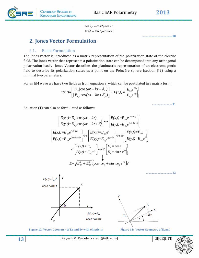
yxoyox .sin.cos.22
……………………………..12
Figure 12: Vector Geometry of Ex and Ey with ellipticity Figure 13: Vector Geometry of Ex and
Basic SAR Polarimetry 2013
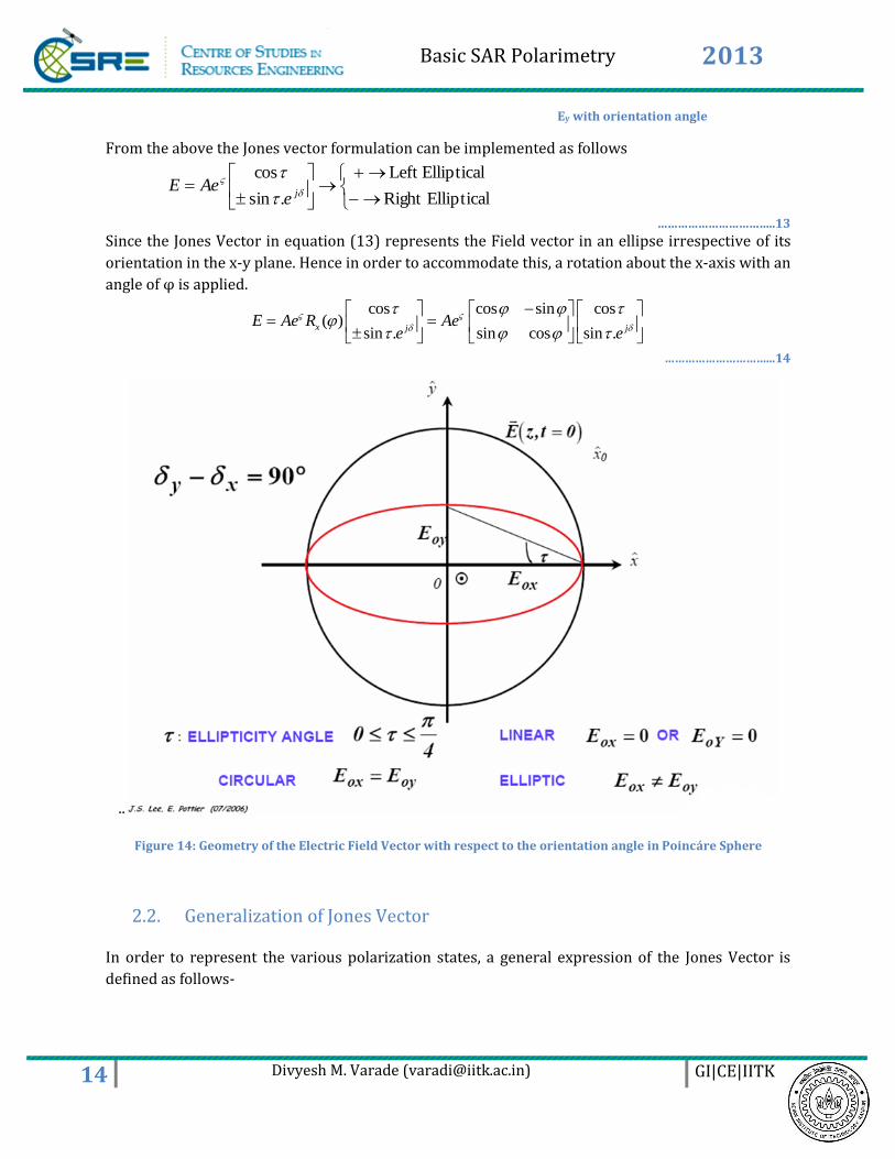
14 Divyesh M. Varade ([email protected]) GI|CE|IITK
Ey with orientation angle
From the above the Jones vector formulation can be implemented as follows
EllipticalRight
EllipticalLeft
.sin
cos
je
AeE
……………………………..13
Since the Jones Vector in equation (13) represents the Field vector in an ellipse irrespective of its
orientation in the x-y plane. Hence in order to accommodate this, a rotation about the x-axis with an
angle of φ is applied.
cos cos sin cos( )
sin . sin cos sin .x j j
E Ae R Aee e
…………………………...14
..
Figure 14: Geometry of the Electric Field Vector with respect to the orientation angle in Poincáre Sphere
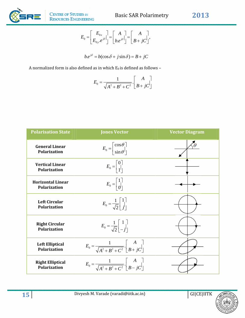
2.2. Generalization of Jones Vector
In order to represent the various polarization states, a general expression of the Jones Vector is
defined as follows-
Basic SAR Polarimetry 2013
15 Divyesh M. Varade ([email protected]) GI|CE|IITK
0
0
0
, . .
. (cos sin )
x
j jy
j
E A AE
E e b e B jC
b e b j B jC
A normalized form is also defined as in which E0 is defined as follows –
02 2 2
1.
AE
B jCA B C
Polarisation State Jones Vector Vector Diagram
General Linear Polarization 0
cos
sinE
Vertical Linear Polarization 0
0
1E
Horizontal Linear Polarization 0
1
0E
Left Circular Polarization 0
11
2E
j
Right Circular Polarization 0
11
2E
j
Left Elliptical Polarization 0
2 2 2
1.
AE
B jCA B C
Right Elliptical Polarization 0
2 2 2
1.
AE
B jCA B C
Basic SAR Polarimetry 2013
16 Divyesh M. Varade ([email protected]) GI|CE|IITK
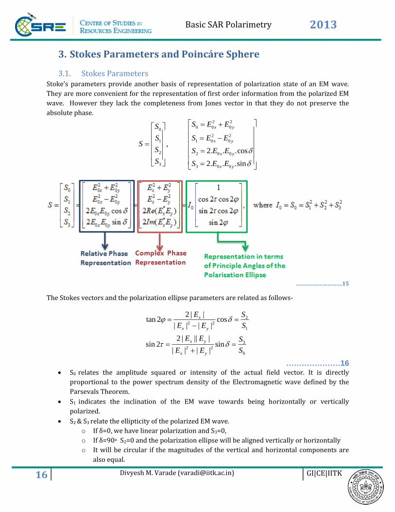
3. Stokes Parameters and Poincáre Sphere
3.1. Stokes Parameters Stoke’s parameters provide another basis of representation of polarization state of an EM wave.
They are more convenient for the representation of first order information from the polarized EM
wave. However they lack the completeness from Jones vector in that they do not preserve the
absolute phase. 2 2
0 0 00
2 2
1 0 01
2 2 0 0
33 0 0
, 2. . .cos
2. . .sin
x y
x y
x y
x y
S E ES
S E ESS
S S E E
S S E E
………………………….15
The Stokes vectors and the polarization ellipse parameters are related as follows-
2
2 2
1
3
2 2
0
2 | |tan 2 cos
| | | |
2 | || |sin 2 sin
| | | |
x
x y
x y
x y
E S
E E S
E E S
E E S
…………………16 S0 relates the amplitude squared or intensity of the actual field vector. It is directly
proportional to the power spectrum density of the Electromagnetic wave defined by the
Parsevals Theorem.
S1 indicates the inclination of the EM wave towards being horizontally or vertically
polarized.
S2 & S3 relate the ellipticity of the polarized EM wave.
o If δ=0, we have linear polarization and S3=0,
o If δ=90o S2=0 and the polarization ellipse will be aligned vertically or horizontally
o It will be circular if the magnitudes of the vertical and horizontal components are
also equal.
Basic SAR Polarimetry 2013
17 Divyesh M. Varade ([email protected]) GI|CE|IITK
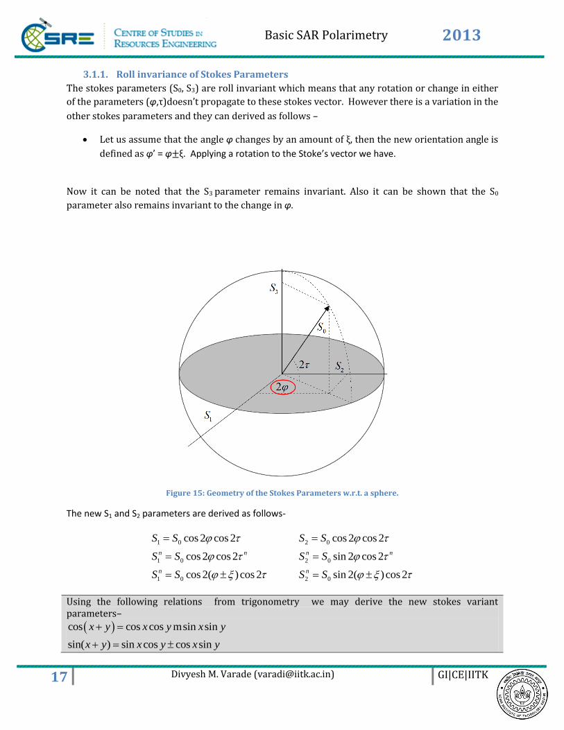
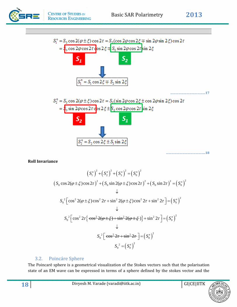
3.1.1. Roll invariance of Stokes Parameters
The stokes parameters (S0, S3) are roll invariant which means that any rotation or change in either
of the parameters (φ,τ)doesn’t propagate to these stokes vector. However there is a variation in the
other stokes parameters and they can derived as follows –
Let us assume that the angle φ changes by an amount of ξ, then the new orientation angle is
defined as φ’ = φ±ξ. Applying a rotation to the Stoke’s vector we have.
Now it can be noted that the S3 parameter remains invariant. Also it can be shown that the S0
parameter also remains invariant to the change in φ.
Figure 15: Geometry of the Stokes Parameters w.r.t. a sphere.
The new S1 and S2 parameters are derived as follows-
1 0
1 0
1 0
cos 2 cos 2
cos 2 cos 2
cos 2( )cos 2
n n
n
S S
S S
S S
2 0
2 0
2 0
cos 2 cos 2
sin 2 cos 2
sin 2( )cos 2
n n
n
S S
S S
S S
Using the following relations from trigonometry we may derive the new stokes variant parameters–
cos cos cos sin sin
sin( ) sin cos cos sin
x y x y x y
x y x y x y
m
Basic SAR Polarimetry 2013
18 Divyesh M. Varade ([email protected]) GI|CE|IITK
…………………………………17
……………………………………..18
Roll Invariance
2 2 2 2
1 2 3 0
22 2 2
0 0 0 0
2 2 2 2 2 2
0
cos 2( )cos 2 sin 2( )cos 2 sin 2
cos 2( )cos 2 sin 2( )cos 2 sin 2
n n n n
n
S S S S
S S S S
S
2
0
2 2 2 2
0
cos 2 cos 2( ) sin 2(
nS
S
2
2
0
2 2 2
0
) sin 2
cos 2 sin 2
nS
S
2
0
22
0 0
n
n
S
S S
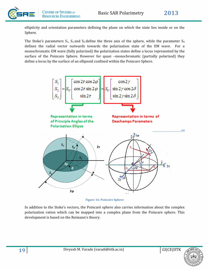
3.2. Poincáre Sphere The Poincarē sphere is a geometrical visualization of the Stokes vectors such that the polarisation
state of an EM wave can be expressed in terms of a sphere defined by the stokes vector and the
Basic SAR Polarimetry 2013
19 Divyesh M. Varade ([email protected]) GI|CE|IITK
ellipticity and orientation parameters defining the plane on which the state lies inside or on the
Sphere.
The Stoke’s parameters S1, S2 and S3 define the three axis of the sphere, while the parameter S0
defines the radial vector outwards towards the polarization state of the EM wave. For a
monochromatic EM wave (fully polarized) the polarization states define a locus represented by the
surface of the Poincare Sphere. However for quasi –monochromatic (partially polarized) they
define a locus by the surface of an ellipsoid confined within the Poincare Sphere.
………………………………19
Figure 16: Poincáre Sphere
In addition to the Stoke’s vectors, the Poincarē sphere also carries information about the complex
polarization ration which can be mapped into a complex plane from the Poincare sphere. This
development is based on the Reimann’s theory.
Basic SAR Polarimetry 2013
20 Divyesh M. Varade ([email protected]) GI|CE|IITK
Table 2: Polarization Parameters for Some Polarization States (Mott, 1986)
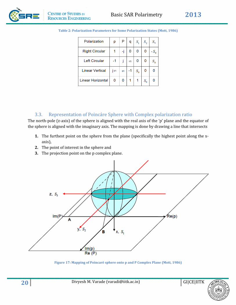
3.3. Representation of Poincáre Sphere with Complex polarization ratio The north-pole (z-axis) of the sphere is aligned with the real axis of the ‘p’ plane and the equator of
the sphere is aligned with the imaginary axis. The mapping is done by drawing a line that intersects
1. The furthest point on the sphere from the plane (specifically the highest point along the x-
axis),
2. The point of interest in the sphere and
3. The projection point on the p complex plane.
Figure 17: Mapping of Poincarē sphere onto p and P Complex Plane (Mott, 1986)
Basic SAR Polarimetry 2013
21 Divyesh M. Varade ([email protected]) GI|CE|IITK
In Figure 17, point A, which is also the north pole of the sphere, describes p=-1 and P= j, which is a
projection from the point (0, 0, S0) of the sphere (with Cartesian coordinates (S1, S2, S3)). Point B
describes p=j and P=1, which is projected from the point (0, 0 S0) from the sphere. This construction
agrees with Table 2. Any other point on the sphere referring to any polarization states can be
mapped in a similar manner (Mott, 1986).
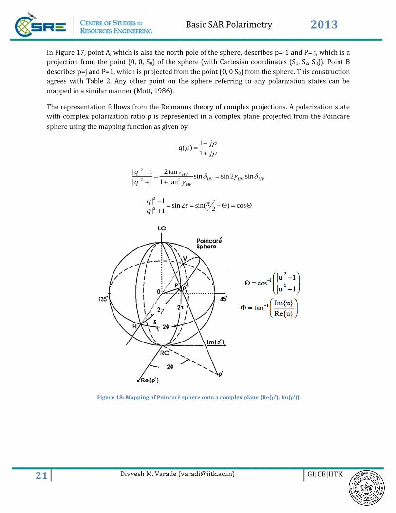
The representation follows from the Reimanns theory of complex projections. A polarization state
with complex polarization ratio ρ is represented in a complex plane projected from the Poincáre
sphere using the mapping function as given by-
1( )
1
jq
j
2
2 2
2tan| | 1sin sin 2 sin
| | 1 1 tan
HVHV HV HV
HV
q
q
2
2
| | 1sin 2 sin( ) cos
2| | 1
q
q
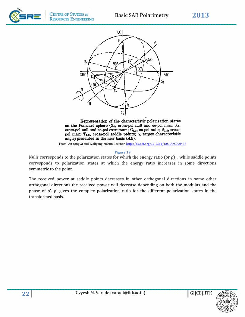
Figure 18: Mapping of Poincarē sphere onto a complex plane {Re(ρ’), Im(ρ’)}
Basic SAR Polarimetry 2013
22 Divyesh M. Varade ([email protected]) GI|CE|IITK
From -An-Qing Xi and Wolfgang-Martin Boerner, http://dx.doi.org/10.1364/JOSAA.9.000437
Figure 19
Nulls corresponds to the polarization states for which the energy ratio (or ρ) , while saddle points
corresponds to polarization states at which the energy ratio increases in some directions
symmetric to the point.
The received power at saddle points decreases in other orthogonal directions in some other
orthogonal directions the received power will decrease depending on both the modulus and the
phase of ρ'. ρ' gives the complex polarization ratio for the different polarization states in the
transformed basis.
Basic SAR Polarimetry 2013
23 Divyesh M. Varade ([email protected]) GI|CE|IITK
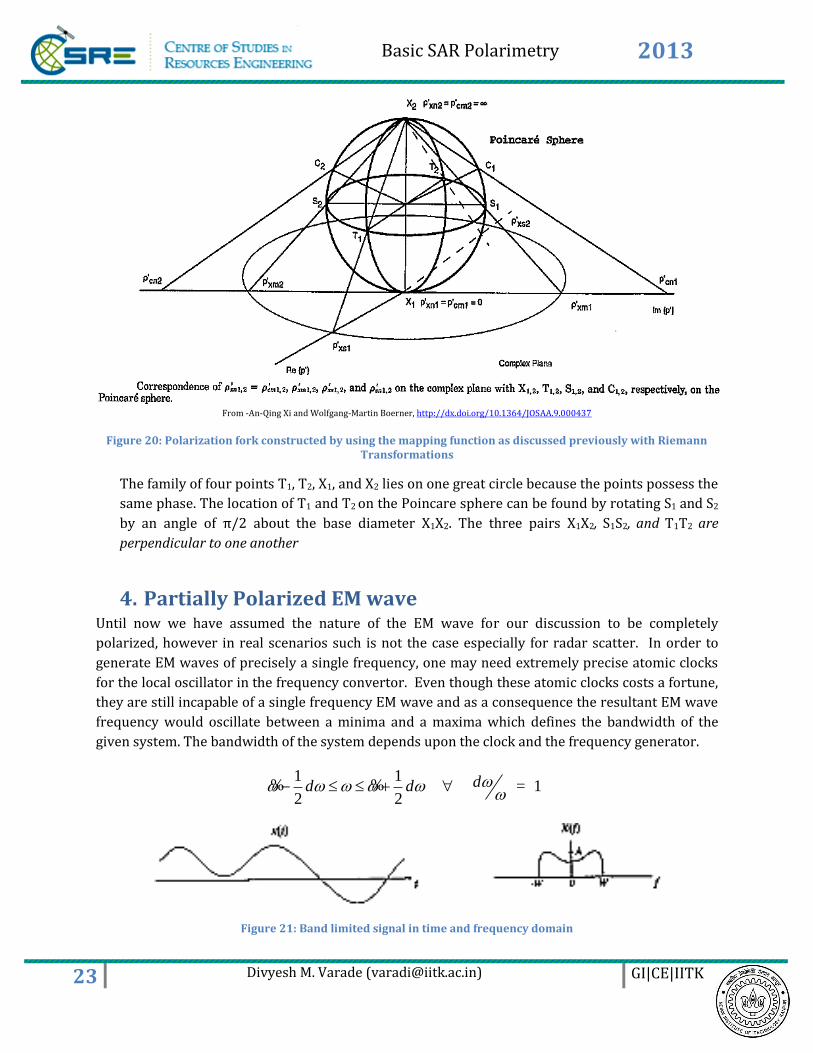
From -An-Qing Xi and Wolfgang-Martin Boerner, http://dx.doi.org/10.1364/JOSAA.9.000437
Figure 20: Polarization fork constructed by using the mapping function as discussed previously with Riemann Transformations
The family of four points T1, T2, X1, and X2 lies on one great circle because the points possess the
same phase. The location of T1 and T2 on the Poincare sphere can be found by rotating S1 and S2
by an angle of π/2 about the base diameter X1X2. The three pairs X1X2, S1S2, and T1T2 are
perpendicular to one another
4. Partially Polarized EM wave Until now we have assumed the nature of the EM wave for our discussion to be completely
polarized, however in real scenarios such is not the case especially for radar scatter. In order to
generate EM waves of precisely a single frequency, one may need extremely precise atomic clocks
for the local oscillator in the frequency convertor. Even though these atomic clocks costs a fortune,
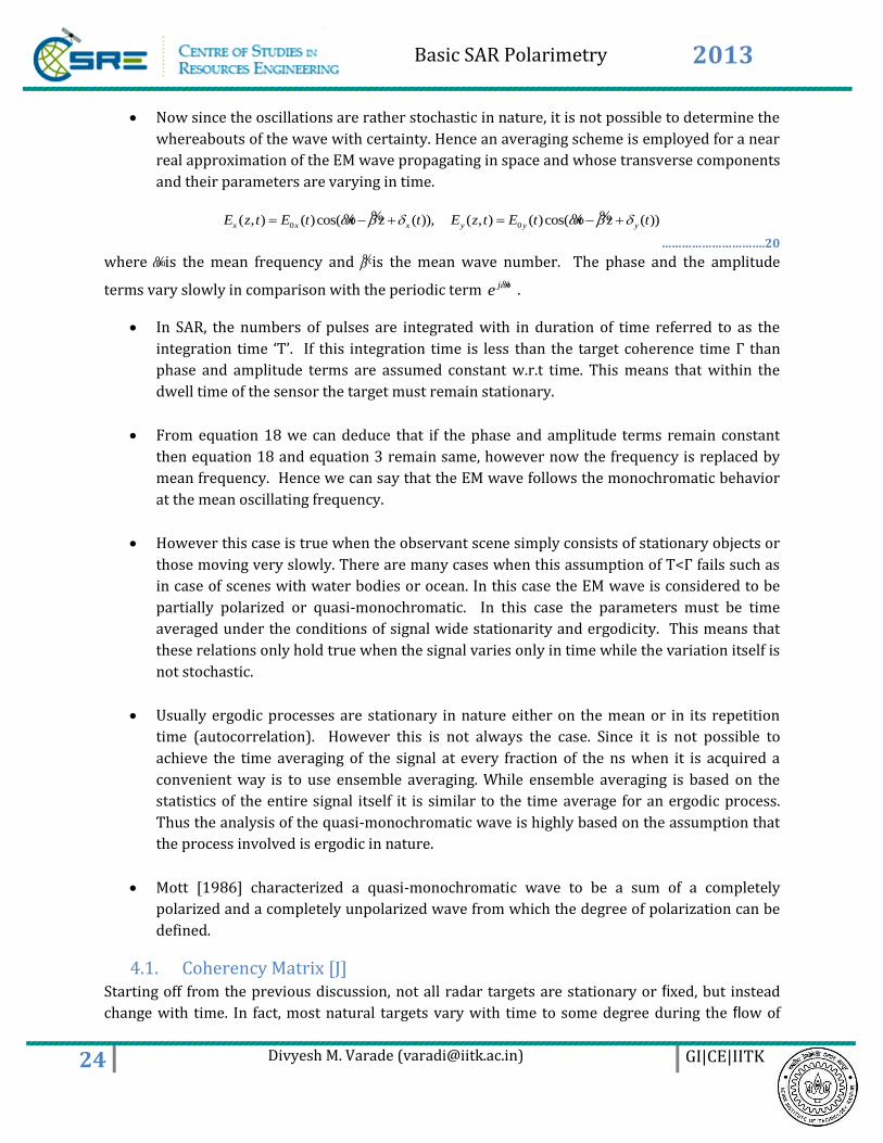
they are still incapable of a single frequency EM wave and as a consequence the resultant EM wave
frequency would oscillate between a minima and a maxima which defines the bandwidth of the
given system. The bandwidth of the system depends upon the clock and the frequency generator.
1 1 1
2 2dd d
% % =
Figure 21: Band limited signal in time and frequency domain
Basic SAR Polarimetry 2013
24 Divyesh M. Varade ([email protected]) GI|CE|IITK
Now since the oscillations are rather stochastic in nature, it is not possible to determine the
whereabouts of the wave with certainty. Hence an averaging scheme is employed for a near
real approximation of the EM wave propagating in space and whose transverse components
and their parameters are varying in time.
0 0( , ) ( )cos( ( )), ( , ) ( )cos( ( ))x x x y y yE z t E t t z t E z t E t t z t % %% %
………………………….20
where %is the mean frequency and %is the mean wave number. The phase and the amplitude
terms vary slowly in comparison with the periodic term j te % .
In SAR, the numbers of pulses are integrated with in duration of time referred to as the
integration time ‘T’. If this integration time is less than the target coherence time Г than
phase and amplitude terms are assumed constant w.r.t time. This means that within the
dwell time of the sensor the target must remain stationary.
From equation 18 we can deduce that if the phase and amplitude terms remain constant
then equation 18 and equation 3 remain same, however now the frequency is replaced by
mean frequency. Hence we can say that the EM wave follows the monochromatic behavior
at the mean oscillating frequency.
However this case is true when the observant scene simply consists of stationary objects or
those moving very slowly. There are many cases when this assumption of T<Г fails such as
in case of scenes with water bodies or ocean. In this case the EM wave is considered to be
partially polarized or quasi-monochromatic. In this case the parameters must be time
averaged under the conditions of signal wide stationarity and ergodicity. This means that
these relations only hold true when the signal varies only in time while the variation itself is
not stochastic.
Usually ergodic processes are stationary in nature either on the mean or in its repetition
time (autocorrelation). However this is not always the case. Since it is not possible to
achieve the time averaging of the signal at every fraction of the ns when it is acquired a
convenient way is to use ensemble averaging. While ensemble averaging is based on the
statistics of the entire signal itself it is similar to the time average for an ergodic process.
Thus the analysis of the quasi-monochromatic wave is highly based on the assumption that
the process involved is ergodic in nature.
Mott [1986] characterized a quasi-monochromatic wave to be a sum of a completely
polarized and a completely unpolarized wave from which the degree of polarization can be
defined.
4.1. Coherency Matrix [J] Starting off from the previous discussion, not all radar targets are stationary or fixed, but instead
change with time. In fact, most natural targets vary with time to some degree during the flow of
Basic SAR Polarimetry 2013
25 Divyesh M. Varade ([email protected]) GI|CE|IITK
wind and stresses generated by temperature or pressure gradients. This generalizes the concept of
‘distributed targets’. Aside from the natural movements of the target, the radar itself may be moving
with respect to the target and illuminating in time the different parts of an extended volume or
surface (Lee and Pottier, 2009).
Now because the wave no longer has the coherent, monochromatic, completely polarized shape of
an elliptically polarized wave; and the state of such a wave is given by the so-called wave
covariance matrix.
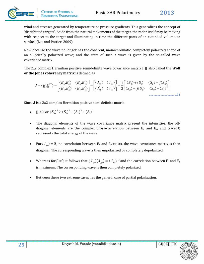
The 2_2 complex Hermitian positive semidefinite wave covariance matrix [ J] also called the Wolf
or the Jones coherency matrix is defined as
* *
0 1 2 3*
** *
2 3 0 1
. . 1.
. . 2
xx xyx x x yT
xy yyy x y y
J J S S S j SE E E EJ E E
J J S j S S SE E E E
………………………………21
Since J is a 2x2 complex Hermitian positive semi definite matrix-
|J|≥0, or 2 2 2 2
0 1 2 3S S S S
The diagonal elements of the wave covariance matrix present the intensities, the off-
diagonal elements are the complex cross-correlation between Ex and Ey, and trace(J)
represents the total energy of the wave.
For 0xyJ , no correlation between Ex and Ey exists, the wave covariance matrix is then
diagonal. The corresponding wave is then unpolarized or completely depolarized.
Whereas for|J|=0, it follows that 2| |xy yy xyJ J J and the correlation between Ex and Ey
is maximum. The corresponding wave is then completely polarized.
Between these two extreme cases lies the general case of partial polarization.
Basic SAR Polarimetry 2013
26 Divyesh M. Varade ([email protected]) GI|CE|IITK
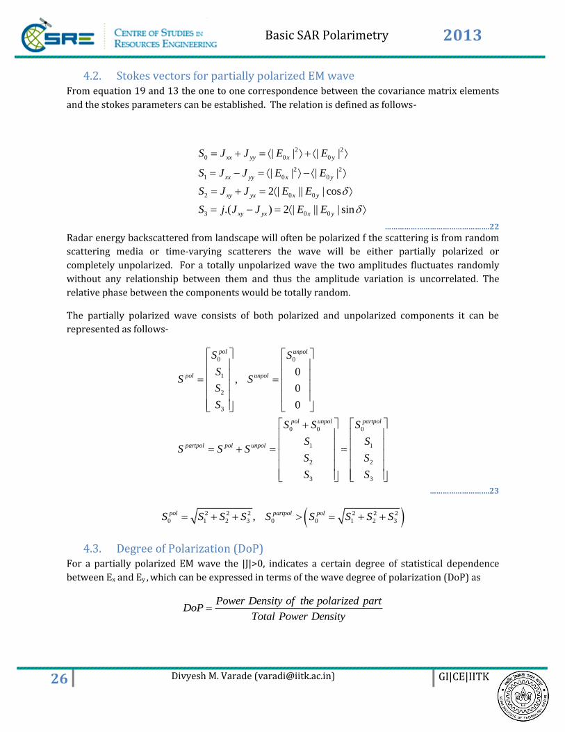
4.2. Stokes vectors for partially polarized EM wave From equation 19 and 13 the one to one correspondence between the covariance matrix elements
and the stokes parameters can be established. The relation is defined as follows-
2 2
0 0 0
2 2
1 0 0
2 0 0
3 0 0
| | | |
| | | |
2 | || | cos
.( ) 2 | || | sin
xx yy x y
xx yy x y
xy yx x y
xy yx x y
S J J E E
S J J E E
S J J E E
S j J J E E
………………………………………….22
Radar energy backscattered from landscape will often be polarized f the scattering is from random
scattering media or time-varying scatterers the wave will be either partially polarized or
completely unpolarized. For a totally unpolarized wave the two amplitudes fluctuates randomly
without any relationship between them and thus the amplitude variation is uncorrelated. The
relative phase between the components would be totally random.
The partially polarized wave consists of both polarized and unpolarized components it can be
represented as follows-
0 0
1
2
3
0 0 0
1 1
2 2
3 3
0,
0
0
pol unpol
pol unpol
pol unpol partpol
partpol pol unpol
S S
SS S
S
S
S S S
S SS S S
S S
S S
……………………….23
2 2 2 2 2 2
0 1 2 3 0 0 1 2 3, pol partpol polS S S S S S S S S
4.3. Degree of Polarization (DoP) For a partially polarized EM wave the |J|>0, indicates a certain degree of statistical dependence
between Ex and Ey , which can be expressed in terms of the wave degree of polarization (DoP) as
Power Density of the polarized partDoP
Total Power Density
Basic SAR Polarimetry 2013
27 Divyesh M. Varade ([email protected]) GI|CE|IITK
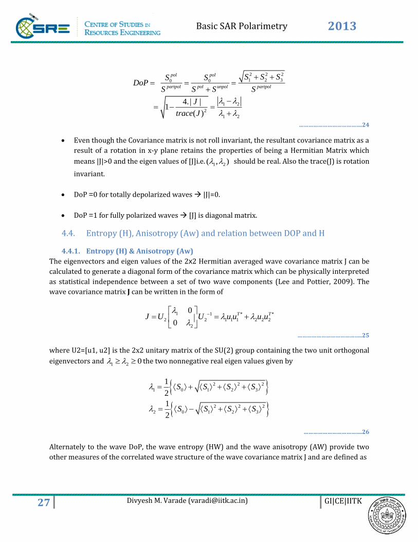
2 2 2
1 2 30 0
1 2
2
1 2
4. | | 1
( )
pol pol
partpol pol unpol partpol
S S SS SDoP
S S S S
J
trace J
………………………………….24
Even though the Covariance matrix is not roll invariant, the resultant covariance matrix as a
result of a rotation in x-y plane retains the properties of being a Hermitian Matrix which
means |J|>0 and the eigen values of [J]i.e.1 2( , ) should be real. Also the trace(J) is rotation
invariant.
DoP =0 for totally depolarized waves |J|=0.
DoP =1 for fully polarized waves [J] is diagonal matrix.
4.4. Entropy (H), Anisotropy (Aw) and relation between DOP and H
4.4.1. Entropy (H) & Anisotropy (Aw)
The eigenvectors and eigen values of the 2x2 Hermitian averaged wave covariance matrix J can be
calculated to generate a diagonal form of the covariance matrix which can be physically interpreted
as statistical independence between a set of two wave components (Lee and Pottier, 2009). The
wave covariance matrix J can be written in the form of
1 1 * *
2 2 1 1 1 2 2 2
2
0
0
T TJ U U u u u u
…………………………………..25
where U2=[u1, u2] is the 2x2 unitary matrix of the SU(2) group containing the two unit orthogonal
eigenvectors and 1 2 0 the two nonnegative real eigen values given by
2 2 2
1 0 1 2 3
2 2 2
2 0 1 2 3
1
2
1
2
S S S S
S S S S
……………………………….26
Alternately to the wave DoP, the wave entropy (HW) and the wave anisotropy (AW) provide two
other measures of the correlated wave structure of the wave covariance matrix J and are defined as
Basic SAR Polarimetry 2013
28 Divyesh M. Varade ([email protected]) GI|CE|IITK
21 2
2
11 2 1 2
, log with ii i i
i
Aw H p p p
………………………….27
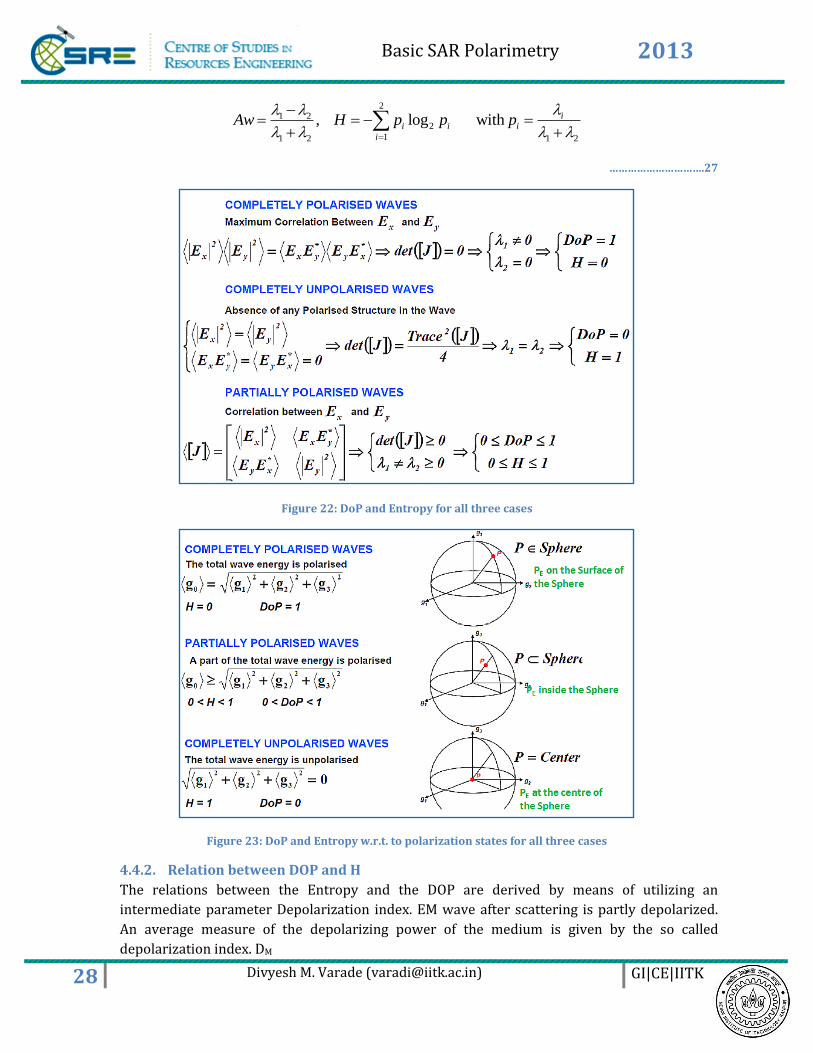
Figure 22: DoP and Entropy for all three cases
Figure 23: DoP and Entropy w.r.t. to polarization states for all three cases
4.4.2. Relation between DOP and H
The relations between the Entropy and the DOP are derived by means of utilizing an
intermediate parameter Depolarization index. EM wave after scattering is partly depolarized.
An average measure of the depolarizing power of the medium is given by the so called
depolarization index. DM
Basic SAR Polarimetry 2013
29 Divyesh M. Varade ([email protected]) GI|CE|IITK
The incident EM wave on a target undergoes a change in polarization. However the received EM
wave has undergone many such alterations. This is due to the inevitable objects in the path such
dust, clouds and majorly the Ionosphere. The Ionosphere contains free electron clouds defined
by TEC. Now these create an apparent electric field which forces the Radar EM wave out of its
polarization state slightly. Thus the Entropy is actually not defined by a function of single
variable but a set of variables (prominently 3). So considering the single alteration the Entropy
and the DOP can be represented by single valued functions. While for the other case they are
defined by multi-valued functions.
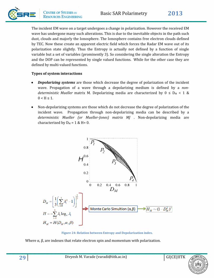
Types of system interactions
Depolarizing systems are those which decrease the degree of polarization of the incident
wave. Propagation of a wave through a depolarizing medium is defined by a non-
deterministic Mueller matrix M. Depolarizing media are characterized by 0 ≤ DM < 1 &
0 < H ≤ 1.
Non-depolarizing systems are those which do not decrease the degree of polarization of the
incident wave. Propagation through non-depolarizing media can be described by a
deterministic Mueller (or Mueller-Jones) matrix MJ . Non-depolarizing media are
characterized by DM = 1 & H= 0.
Figure 24: Relation between Entropy and Depolarization index.
Where α, β, are indexes that relate electron spin and momentum with polarization.
Basic SAR Polarimetry 2013
30 Divyesh M. Varade ([email protected]) GI|CE|IITK
5. Change of Polarimetric Basis
5.1. Special Unitary decomposition of E vector
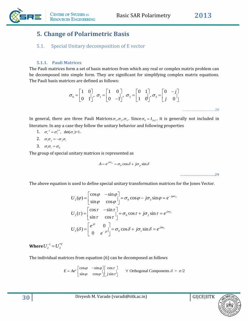
5.1.1. Pauli Matrices
The Pauli matrices form a set of basis matrices from which any real or complex matrix problem can
be decomposed into simple form. They are significant for simplifying complex matrix equations.
The Pauli basis matrices are defined as follows:
0 1 2 3
1 0 1 0 0 1 0, , ,
0 1 0 1 1 0 0
j
j
………………………………28
In general, there are three Pauli Matrices 1 2 3, , . Since 0 2x2I , it is generally not included in
literature. In any a case they follow the unitary behavior and following properties
1. 1 *, det( )=1T
i i i .
2. i j j i
3. 0i i
The group of special unitary matrices is represented as
0 cos sinpj
pA e j
……………………………….29
The above equation is used to define special unitary transformation matrices for the Jones Vector.
3
3
1
2 0 3
2 0 2
2 0 1
cos sin( ) cos sin
sin cos
cos sin( ) cos sin
sin cos
0( ) cos sin
0
j
j
j
j
j
U j e
U j e
eU j e
e
Where1 *
2 2
TU U
The individual matrices from equation (6) can be decomposed as follows
cos sin cos Orthogonal Components = /2
sin cos sinE Ae
j
Basic SAR Polarimetry 2013
31 Divyesh M. Varade ([email protected]) GI|CE|IITK
cos sin cos sin 1
sin cos sin cos 0
jE Ae
j
cos sin cos sin 10
sin cos sin cos 00
j eE A
j e
…………………………30 3 2 1
2 2 2 2ˆ ˆ ˆ( ) ( ) ( ) ( , , )
j j j
x x xAU U U u AU u Ae e e u
Where ˆxu corresponds to the x-component of the unit Jones vector. By using this decomposition we
can see that the dimensionality of the original vector E has reduced. By using the complex rotation
(special unitary) removes the addendum phase carried through by the EM wave.
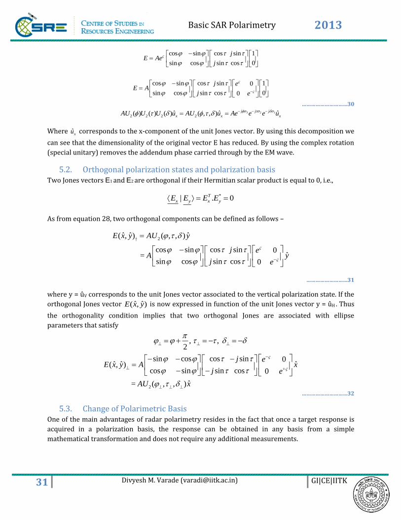
5.2. Orthogonal polarization states and polarization basis Two Jones vectors E1 and E2 are orthogonal if their Hermitian scalar product is equal to 0, i.e.,
*| . 0T
x y x yE E E E
As from equation 28, two orthogonal components can be defined as follows –
|ˆ ˆ( , )E x y 2
ˆ( , , )
cos sin cos sin 0ˆ =
sin cos sin cos 0
AU y
j eA y
j e
………………………31
where y = ûV corresponds to the unit Jones vector associated to the vertical polarization state. If the
orthogonal Jones vector ˆ ˆ( , )E x y is now expressed in function of the unit Jones vector y = ûH . Thus
the orthogonality condition implies that two orthogonal Jones are associated with ellipse
parameters that satisfy
, , 2
2
sin cos cos sin 0ˆ ˆ ˆ( , )
cos sin sin cos 0
ˆ = ( , , )
j eE x y A x
j e
AU x
…………………………32
5.3. Change of Polarimetric Basis One of the main advantages of radar polarimetry resides in the fact that once a target response is
acquired in a polarization basis, the response can be obtained in any basis from a simple
mathematical transformation and does not require any additional measurements.
Basic SAR Polarimetry 2013
32 Divyesh M. Varade ([email protected]) GI|CE|IITK
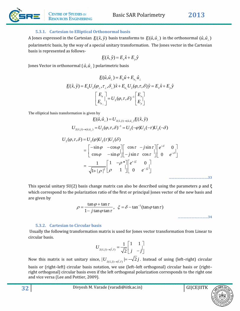
5.3.1. Cartesian to Elliptical Orthonormal basis
A Jones expressed in the Cartesian ˆ ˆ( , )E x y basis transforms to ˆ ˆ( , )E u u in the orthonormal ˆ ˆ( , )u u
polarimetric basis, by the way of a special unitary transformation. The Jones vector in the Cartesian
basis is represented as follows-
ˆ ˆ ˆ ˆ( , ) x yE x y E x E y
Jones Vector in orthonormal ( ˆ ˆ,u u) polarimetric basis
ˆ ˆ ˆ ˆ( , ) u uE u u E u E u
2 2ˆ ˆ ˆ ˆ ˆ ˆ( , ) ( , , ) ( , , )u u x yE x y E U x E U y E x E y
1
2 ( , , )u x
u y
E EU
E E
The elliptical basis transformation is given by
ˆ ˆ ˆ ˆ2( , ) ( , )ˆ ˆ ˆ ˆ( , ) ( , )x y u uE u u U E x y
1
ˆ ˆ ˆ ˆ2( , ) ( , ) 2 2 2 2( , , ) ( ) ( ) ( )x y u uU U U U U
2 2 2 2
2
( , , ) ( ) ( ) ( )
sin cos cos sin 0 =
cos sin sin cos 0
1 * 01 =
1 01 | |
j
j
U U U U
j e
j e
e
e
…………………………………….33
This special unitary SU(2) basis change matrix can also be described using the parameters ρ and ξ
which correspond to the polarization ratio of the first or principal Jones vector of the new basis and
are given by
1tan tan, tan (tan tan )
1 tan tanj
……………………………34
5.3.2. Cartesian to Circular basis
Usually the following transformation matrix is used for Jones vector transformation from Linear to
circular basis.
ˆˆ ˆ ˆ2( , ) ( , )
1 11
2x y l r
Uj j
Now this matrix is not unitary since, ˆˆ ˆ ˆ2( , ) ( , )| | 2
x y l rU j
. Instead of using (left–right) circular
basis or (right–left) circular basis notation, we use (left–left orthogonal) circular basis or (right–right orthogonal) circular basis even if the left orthogonal polarization corresponds to the right one and vice versa (Lee and Pottier, 2009).
Basic SAR Polarimetry 2013
33 Divyesh M. Varade ([email protected]) GI|CE|IITK
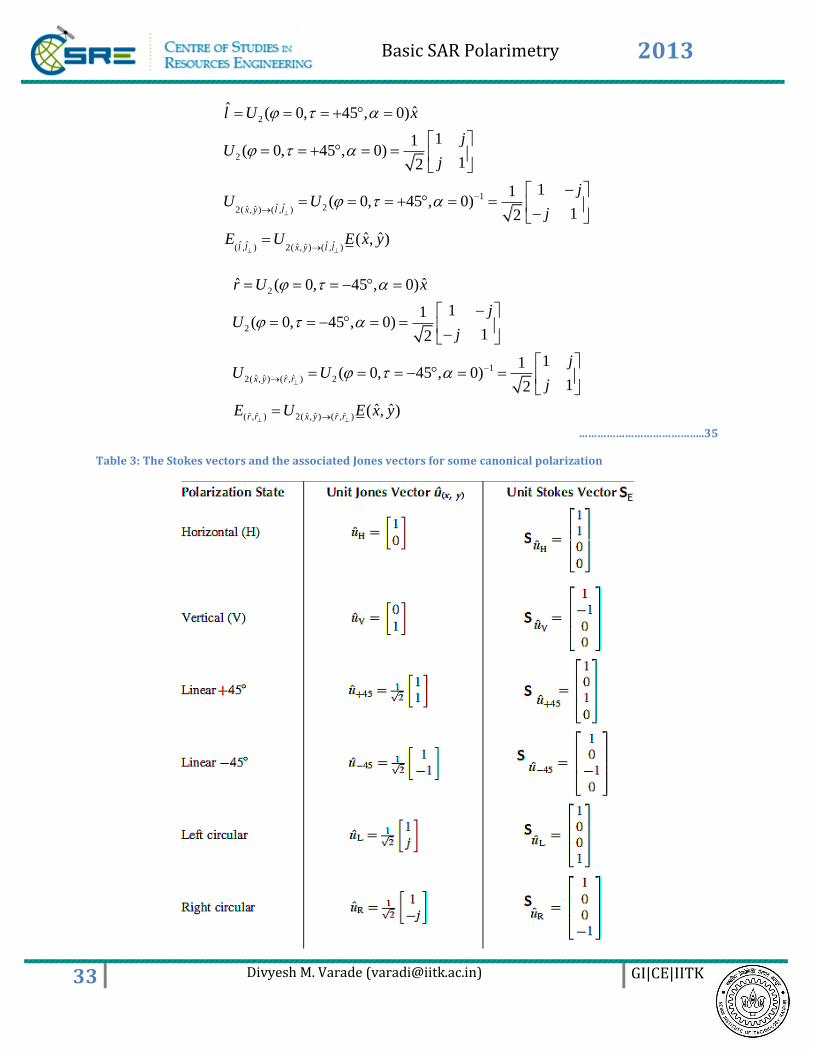
2
2
1
ˆ ˆ 2ˆ ˆ2( , ) ( , )
ˆ ˆ ˆ ˆˆ ˆ( , ) 2( , ) ( , )
ˆ ˆ( 0, 45 , 0)
11( 0, 45 , 0)
12
11( 0, 45 , 0)
12
ˆ ˆ( , )
x y l l
l l x y l l
l U x
jU
j
jU U
j
E U E x y
2
2
1
ˆ ˆ ˆ ˆ2( , ) ( , ) 2
ˆ ˆ ˆ ˆ ˆ ˆ( , ) 2( , ) ( , )
ˆ ˆ( 0, 45 , 0)
11( 0, 45 , 0)
12
11( 0, 45 , 0)
12
ˆ ˆ( , )
x y r r
r r x y r r
r U x
jU
j
jU U
j
E U E x y
…………………………………..35
Table 3: The Stokes vectors and the associated Jones vectors for some canonical polarization
Basic SAR Polarimetry 2013
34 Divyesh M. Varade ([email protected]) GI|CE|IITK
6. Complex Polarization Ratio The polarization of a wave can also be described by the complex polarization ratio.
ox
j
oy
E(x,t)= EE
E(y,t)= E e
tanoy j j
ox
EE(y,t)e e
E(x,t) E
……………………………..36
Now from the Jones vectors we have
cos sin cos
sin cos sinE Ae
j
From equation 10, it follows
cos sin cos cos cos sin sin
sin cos sin sin cos cos sin
cos cos sin sin 1 tan tan by cos cos
sin cos cos sin tan tan
j
j j
j j
j j
tan tan
1 tan tan
j
j
6.1.1. Complex Polarization Ratio in an arbitrary basis Any wave can be resolved into two orthogonal components (linearly, circularly, or elliptically
polarized) in the plane transverse to the direction of propagation. For an arbitrary polarization
basis {A B} with unit vectors ˆˆ and a b .
ˆˆ( ) A BE AB E a E b
{ ( )}| || |
| |A B ABj jB B
AB AB
A A
E Ee e
E E
…………………………….37
where EA and EB are complex numbers.AB is also a complex number.
coscos tan
cossin .
1cos Let 1
j
j
AB
AB
E E E ee
E E E
1 12 *
2 *2 2 *
1tan = cos 1 1
1
B A B B B
A AA AA B AB AB
E E E E E
E EE EE E
*
11
1 ABAB AB
E
………………………....38
Basic SAR Polarimetry 2013
35 Divyesh M. Varade ([email protected]) GI|CE|IITK
6.1.2. Complex polarization ratio in the linear basis {H V} In the linear {HV} basis, a polarization state (Fig. 12) may be expressed as
ˆ ˆ( ) H VE HV E h E v
2 2| |
| | cos
| | sin
H H
H HV
V HV
E E E
E E
E E
Then the complex polarization ratio for the {HV} basis is expressed as follows-
| |
tan . ,| |
HV HVj jV VHV HV HV H V
H H
E Ee e
E E
……………………………39
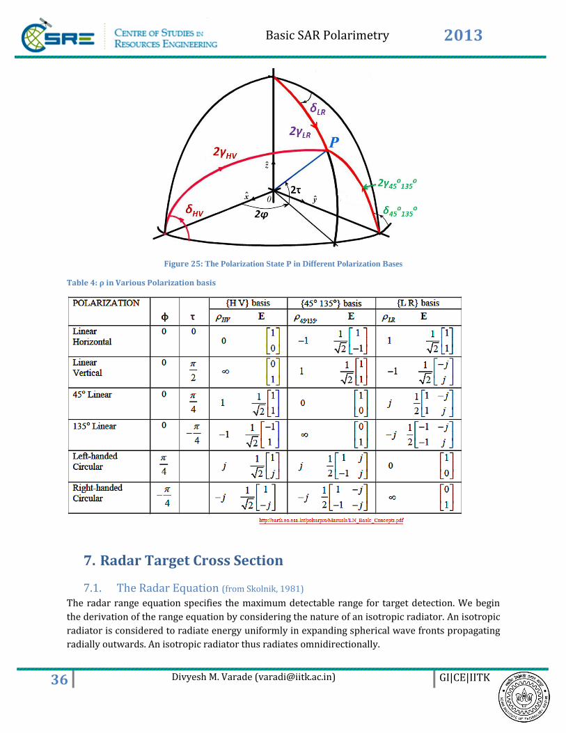
where the parameters ( , ) are the Deschamp’s parameters (Fig. 10). Section 2.1 provides the
basic formulation of the Jones representation of a TEM wave propagating in the z-direction. In Fig.
10, the polarization state, described by the point P E on the Poincaré sphere, can be expressed in terms of
these two angles, where 2γ is the angle subtended by the great circle drawn from the point P E on the
equator measured from H towards V; and δ is the angle between the great circle and the equator. Equation
7 describes the relation between the δ and (φ,τ).
6.1.3. Complex polarization ratio in the circular basis {L, R}
In the circular basis {L R}, we have two unit vectors L̂ (Left handed circular) and R̂ (Right handed
Circular). Any polarization of a plane wave can be expressed by
ˆ ˆ( ) L RE LR E l E r
A unit amplitude left-handed circular polarization has only the L component in the circular basis {L R}. It
can be expressed by ˆ ˆ( ) 1. 0. 1 0T
E LR l r .
A unit amplitude left-handed circular polarization has only the R component in the circular basis {L R}. It
can be expressed by ˆ ˆ( ) 0. 1. 0 1T
E LR l r .
The complex polarization ratio for the {LR} basis is then given by-
{ ( )}| || | tan .
| |R L LR LRj j jR R
LR LR LR
L L
E Ee e e
E E
………………………….40
6.1.4. Complex polarization ratio in the linear basis {45° 135°}
In the linear · ·{45 ,135 } , a polarization state may be expressed as
· · · ·45 13545 ,135 ) 45 1( 35E E E
135 45 45 135 45 135{ (135 13545 135
)
5 5
}
4 4
| || | tan .
| |
jj j
LR LR
E Ee e e
E E
……………………..41
Basic SAR Polarimetry 2013
36 Divyesh M. Varade ([email protected]) GI|CE|IITK
Figure 25: The Polarization State P in Different Polarization Bases
Table 4: ρ in Various Polarization basis
7. Radar Target Cross Section
7.1. The Radar Equation (from Skolnik, 1981) The radar range equation specifies the maximum detectable range for target detection. We begin
the derivation of the range equation by considering the nature of an isotropic radiator. An isotropic
radiator is considered to radiate energy uniformly in expanding spherical wave fronts propagating
radially outwards. An isotropic radiator thus radiates omnidirectionally.
Basic SAR Polarimetry 2013
37 Divyesh M. Varade ([email protected]) GI|CE|IITK
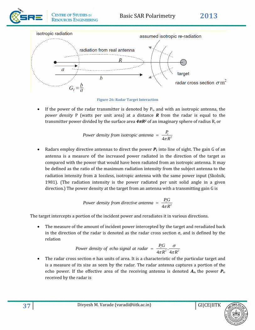
Figure 26: Radar Target Interaction
If the power of the radar transmitter is denoted by Pt, and with an isotropic antenna, the
power density P (watts per unit area) at a distance R from the radar is equal to the
transmitter power divided by the surface area 4πR2 of an imaginary sphere of radius R, or
2
4
tPPower density from isotropic antenna
R
Radars employ directive antennas to direct the power Pt into line of sight. The gain G of an
antenna is a measure of the increased power radiated in the direction of the target as
compared with the power that would have been radiated from an isotropic antenna. It may
be defined as the ratio of the maximum radiation intensity from the subject antenna to the
radiation intensity from a lossless, isotropic antenna with the same power input (Skolnik,
1981). (The radiation intensity is the power radiated per unit solid angle in a given
direction.) The power density at the target from an antenna with a transmitting gain G is
2 4
tPower density from directive antenP
nG
aR
The target intercepts a portion of the incident power and reradiates it in various directions.
The measure of the amount of incident power intercepted by the target and reradiated back
in the direction of the radar is denoted as the radar cross section ς, and is defined by the
relation
2 2 .
4 4
tPGPower density of echo signal at radar
R R
The radar cross section ς has units of area. It is a characteristic of the particular target and
is a measure of its size as seen by the radar. The radar antenna captures a portion of the
echo power. If the effective area of the receiving antenna is denoted Ae, the power Pr,
received by the radar is
Basic SAR Polarimetry 2013
38 Divyesh M. Varade ([email protected]) GI|CE|IITK
2 2 2 4 . .
4 4 (4 )
t t er e
PG PG AP A
R R R
…………………………42
The maximum radar range Rmax is the distance beyond which the target cannot be detected.
It occurs when the received echo signal power Pr, just equals the minimum detectable signal
Smin.Therefore 1
4
max 2
min
(4 )
t ePG AR
S
………………………..43
If the transmitting and receiving antenna are same or have same gain, then
2
4G
, and
1 12 2 24 4
max 3 2
min min
(4 ) 4
t t ePG P AR
S S
…………………………44
7.2. Radar Target Cross-Section [RCS] The radar cross section of a target is the (fictional) area intercepting that amount of power which
when scattered equally in all directions, produces an echo at the radar equal to that from the target.
2
2power reflected toward source/unit solid anglelim 4 R .
incident power density4
r
Ri
E
E
…………………………..45
where
R = distance between radar and target
Er, = reflected field strength at radar
Ei = strength of incident field at target
RCS has dimensions of area (orthogonal to the incident radiation). RCS is described by
ς[m]2 .
For most common types of radar targets such as aircraft, ships, and terrain, the radar cross
section does not necessarily bear a simple relationship to the physical area, except that the
larger the target size, the larger the cross section is likely to be.
Usually not easily related to any physical cross sectional area of the target. If the radar
rotates w.r.t the incoming radar beam, then it will have a different RCS defined by the
implicit area needed at that orientation to account for the energy extracted from the
wavefront and re-radiated back to the radar set isotropically.
From equation 43, if we take several measurements of received power with different
orientations of the target, we would then be able to build up a picture of how the RCS of an
object changes with the angle with which it is viewed.
Basic SAR Polarimetry 2013
39 Divyesh M. Varade ([email protected]) GI|CE|IITK
R in equation 45, shows that the radar cross section is measured in the far field. It is
observed that the far field states are more stable than the near field states. Due to the
presence of running electrons in the near field the original EM wave is put through a stray
electric field which causes its deviation from the intended path.
The RCS value can extend over an enormous range (less than 0.01sq.m. to 100sq.m.). It is
usual to express RCS in decibels (dB) w.r.t. some reference level using the definition
2 2
1010log 1 ; 1ref
ref
m m
The unit of RCS is then dBm2.
2
10
2
10log [ ]1
dBmm
7.3. Distributed Targets Some targets in radar remote sensing are of the nature of discrete scatterers. More common
scattering takes place from regions on the Earth’s surface that are distributed in nature (area of
soil/snow/agricultural field/ocean surface). To accommodate these cover types, the radar equation
needs to be modified, commencing with a variation to the definition of RCS.
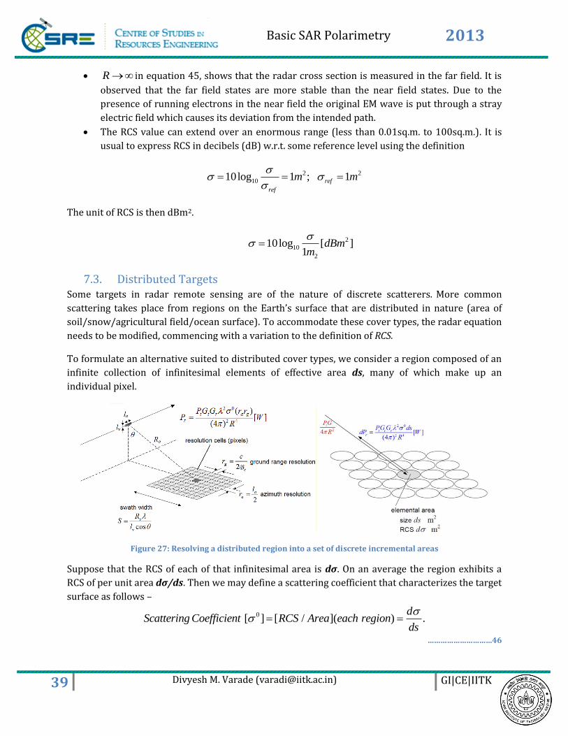
To formulate an alternative suited to distributed cover types, we consider a region composed of an
infinite collection of infinitesimal elements of effective area ds, many of which make up an
individual pixel.
Figure 27: Resolving a distributed region into a set of discrete incremental areas
Suppose that the RCS of each of that infinitesimal area is dσ. On an average the region exhibits a
RCS of per unit area dσ/ds. Then we may define a scattering coefficient that characterizes the target
surface as follows –
0 . [ ] [ / ]( )Scattering Coefficient RCS Area each regd
ons
id
…………………………46
Basic SAR Polarimetry 2013
40 Divyesh M. Varade ([email protected]) GI|CE|IITK
The power received back at the platform after scattering from one of the incremental regions in
terms of scattering coefficient is given by- 2 0
2 4[ ]
(4 )
t t rr
PG G dsdP W
R
…………………………..47
We can now find the total power returned to the platform from a particular resolution cell or pixel
by integrating equation 47. If the parameters are considered as constants in equation then
𝑑𝑠 = 𝑆 = 𝑟𝑎𝑟𝑔 as shown in equation 48
2 02 0
2 4 2 4
( )[ ] [ ]
(4 ) (4 )ij
t t r a gt t rr
s
PG G r rPG G dsP W W
R R
……………………………..48
ς0 describes the ‘tone’ of the radar image and is analogous to the reflectance of Earth surface
materials at visible and infrared wavelengths used in optical Remote Sensing. It is important to
relate ς0 to the physical properties of the region being imaged – its composition, water contents,
physical properties and so on. Like RCS, the scattering coefficient is expressed in decibels (dB)
00
10 2 2[ ] 10log
1dB
m m
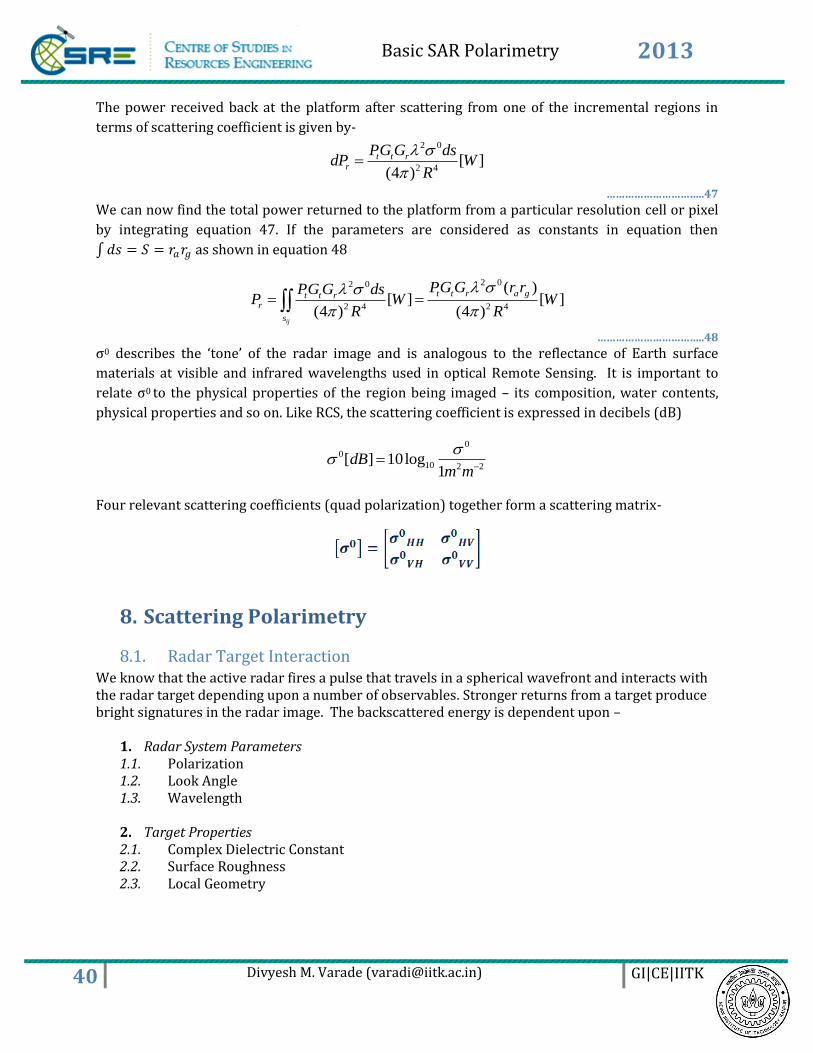
Four relevant scattering coefficients (quad polarization) together form a scattering matrix-
8. Scattering Polarimetry
8.1. Radar Target Interaction We know that the active radar fires a pulse that travels in a spherical wavefront and interacts with the radar target depending upon a number of observables. Stronger returns from a target produce bright signatures in the radar image. The backscattered energy is dependent upon –
1. Radar System Parameters 1.1. Polarization 1.2. Look Angle 1.3. Wavelength 2. Target Properties 2.1. Complex Dielectric Constant 2.2. Surface Roughness 2.3. Local Geometry
Basic SAR Polarimetry 2013
41 Divyesh M. Varade ([email protected]) GI|CE|IITK
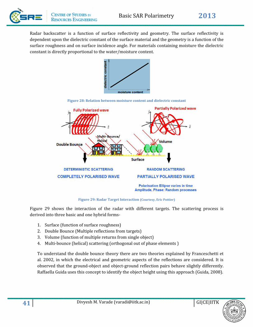
Radar backscatter is a function of surface reflectivity and geometry. The surface reflectivity is
dependent upon the dielectric constant of the surface material and the geometry is a function of the
surface roughness and on surface incidence angle. For materials containing moisture the dielectric
constant is directly proportional to the water/moisture content.
Figure 28: Relation between moisture content and dielectric constant
Figure 29: Radar Target Interaction (Courtesy, Eric Pottier)
Figure 29 shows the interaction of the radar with different targets. The scattering process is
derived into three basic and one hybrid forms-
1. Surface (function of surface roughness)
2. Double Bounce (Multiple reflections from targets)
3. Volume (function of multiple returns from single object)
4. Multi-bounce (helical) scattering (orthogonal out of phase elements )
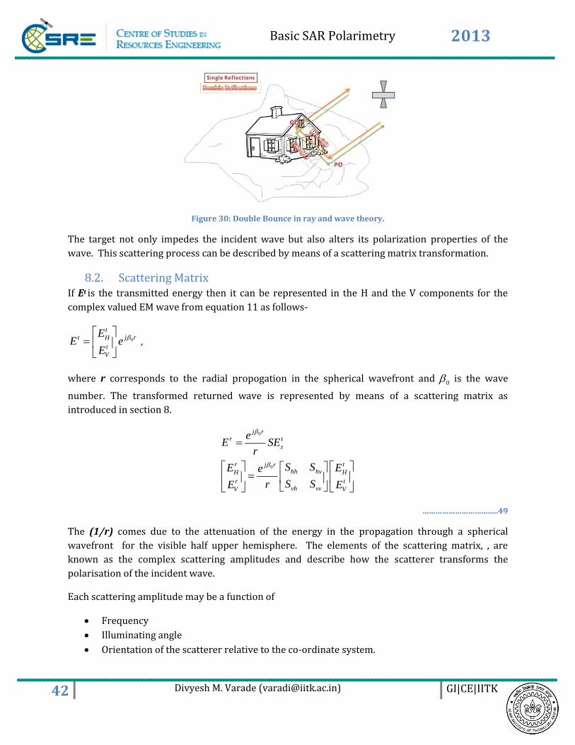
To understand the double bounce theory there are two theories explained by Franceschetti et
al. 2002, in which the electrical and geometric aspects of the reflections are considered. It is
observed that the ground-object and object-ground reflection pairs behave slightly differently.
Raffaella Guida uses this concept to identify the object height using this approach (Guida, 2008).
Basic SAR Polarimetry 2013
42 Divyesh M. Varade ([email protected]) GI|CE|IITK
Figure 30: Double Bounce in ray and wave theory.
The target not only impedes the incident wave but also alters its polarization properties of the
wave. This scattering process can be described by means of a scattering matrix transformation.
8.2. Scattering Matrix If Et is the transmitted energy then it can be represented in the H and the V components for the
complex valued EM wave from equation 11 as follows-
0
t
j rt H
t
V
EE e
E
,
where r corresponds to the radial propogation in the spherical wavefront and 0 is the wave
number. The transformed returned wave is represented by means of a scattering matrix as
introduced in section 8.
0
0
j rr t
z
r tj rhh hvH H
r tvh vvV V
eE SE
r
S SE Ee
S SrE E
……………………………..49
The (1/r) comes due to the attenuation of the energy in the propagation through a spherical
wavefront for the visible half upper hemisphere. The elements of the scattering matrix, , are
known as the complex scattering amplitudes and describe how the scatterer transforms the
polarisation of the incident wave.
Each scattering amplitude may be a function of
Frequency
Illuminating angle
Orientation of the scatterer relative to the co-ordinate system.
Basic SAR Polarimetry 2013
43 Divyesh M. Varade ([email protected]) GI|CE|IITK
8.3. Reciprocity Theorem The theorem of reciprocity states that the two cross-polar terms are equal.
hv vh xS S S:
Targets whose internal state is unaltered (stationary and coherent) by the polarisation of the
probing wave are expected to be the case for most naturally occurring scatterers. Real data may not
always obey the reciprocity theorem exactly due to statistical fluctuations and measurement errors.
The cross-polar term, is often taken as the average of the two and multiplied by 2 to conserve the
total power in the vector, and is performed to reduce the statistical non equality found in real data.
8.4. Scattering Theory The signal measured by the radar system will be the resulting signal of many individual scattered
waves over a distributed target area or volume. A natural target will not be a single pure scatterer
and the target area may have a significant surface roughness or volume scattering component.
The measured scattering matrix will therefore represent a statistical property of the target location.
We generally consider the case of incoherent scattering, which is usually the case for the natural
environment where the reciprocity theorem may not hold true. Incoherent scattering assumes that
the signal for a given target location is comprised of returns from an unknown number of individual
waves. The magnitude and phase are determined by the many individual point conditions
Distance to target,
Surface angle
Material type
Polarising orientation
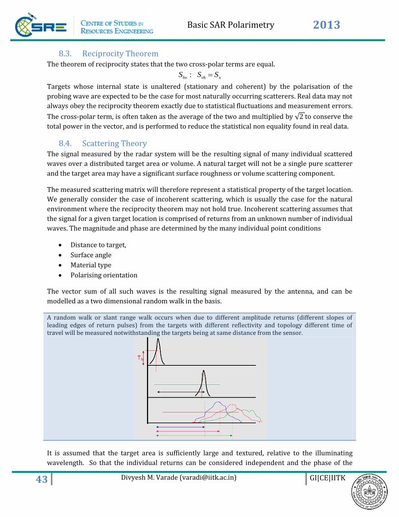
The vector sum of all such waves is the resulting signal measured by the antenna, and can be
modelled as a two dimensional random walk in the basis.
A random walk or slant range walk occurs when due to different amplitude returns (different slopes of leading edges of return pulses) from the targets with different reflectivity and topology different time of travel will be measured notwithstanding the targets being at same distance from the sensor.
It is assumed that the target area is sufficiently large and textured, relative to the illuminating
wavelength. So that the individual returns can be considered independent and the phase of the
Basic SAR Polarimetry 2013
44 Divyesh M. Varade ([email protected]) GI|CE|IITK
vector sum can be considered uniformly random. The central limit theorem implies that when the
number of individual scattering points per resolution cell is very large and the scattering medium is
homogeneous. The scattering process would be Gaussian distributed. However this assumption
does not hold true in many cases especially when observing urban areas or mountainous regions
with fewer peaks and many undulations. In general, if the scattering medium is not spatially
homogeneous, or the resolution cell is not sufficiently large that the central limit theorem applies
then the distribution may be non-Gaussian.
The random phase means that this value is evenly shared between the real and imaginary returned
signal i.e., the magnitude and phase will have equal average intensity, and thus the individual values
will be uncorrelated. Since they vary between positive and negative values indefinitely, it may be
assumed that the mean for their distribution must remain centred in the proximity of zero.
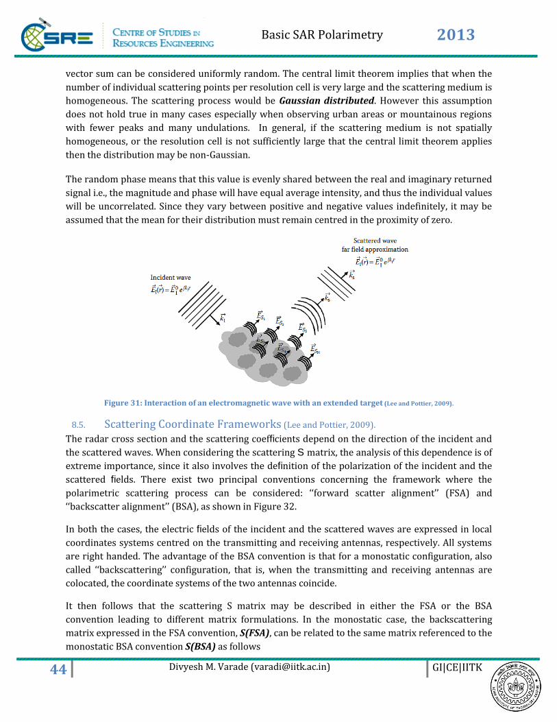
Figure 31: Interaction of an electromagnetic wave with an extended target (Lee and Pottier, 2009).
8.5. Scattering Coordinate Frameworks (Lee and Pottier, 2009).
The radar cross section and the scattering coefficients depend on the direction of the incident and
the scattered waves. When considering the scattering S matrix, the analysis of this dependence is of
extreme importance, since it also involves the definition of the polarization of the incident and the
scattered fields. There exist two principal conventions concerning the framework where the
polarimetric scattering process can be considered: ‘‘forward scatter alignment’’ (FSA) and
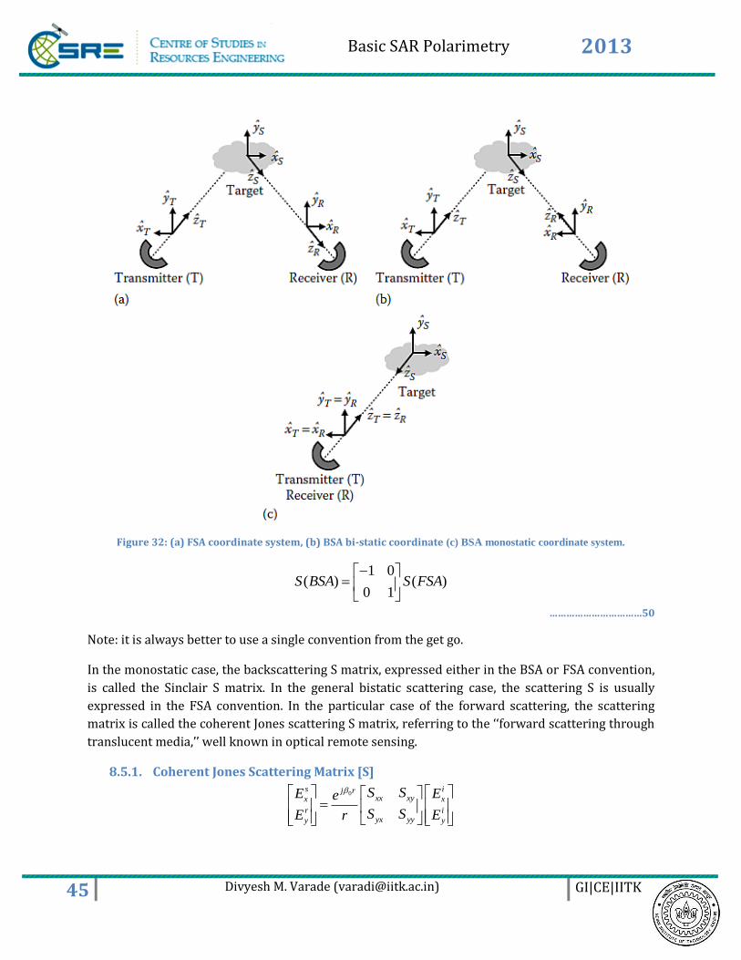
‘‘backscatter alignment’’ (BSA), as shown in Figure 32.
In both the cases, the electric fields of the incident and the scattered waves are expressed in local
coordinates systems centred on the transmitting and receiving antennas, respectively. All systems
are right handed. The advantage of the BSA convention is that for a monostatic configuration, also
called ‘‘backscattering’’ configuration, that is, when the transmitting and receiving antennas are
colocated, the coordinate systems of the two antennas coincide.
It then follows that the scattering S matrix may be described in either the FSA or the BSA
convention leading to different matrix formulations. In the monostatic case, the backscattering
matrix expressed in the FSA convention, S(FSA), can be related to the same matrix referenced to the
monostatic BSA convention S(BSA) as follows
Basic SAR Polarimetry 2013
45 Divyesh M. Varade ([email protected]) GI|CE|IITK
Figure 32: (a) FSA coordinate system, (b) BSA bi-static coordinate (c) BSA monostatic coordinate system.
1 0( ) ( )
0 1S BSA S FSA
……………………………50
Note: it is always better to use a single convention from the get go.
In the monostatic case, the backscattering S matrix, expressed either in the BSA or FSA convention,
is called the Sinclair S matrix. In the general bistatic scattering case, the scattering S is usually
expressed in the FSA convention. In the particular case of the forward scattering, the scattering
matrix is called the coherent Jones scattering S matrix, referring to the ‘‘forward scattering through
translucent media,’’ well known in optical remote sensing.
8.5.1. Coherent Jones Scattering Matrix [S]
0s ij r
xx xyx x
r iyx yyy y
S SE Ee
S SE Er
Basic SAR Polarimetry 2013
46 Divyesh M. Varade ([email protected]) GI|CE|IITK
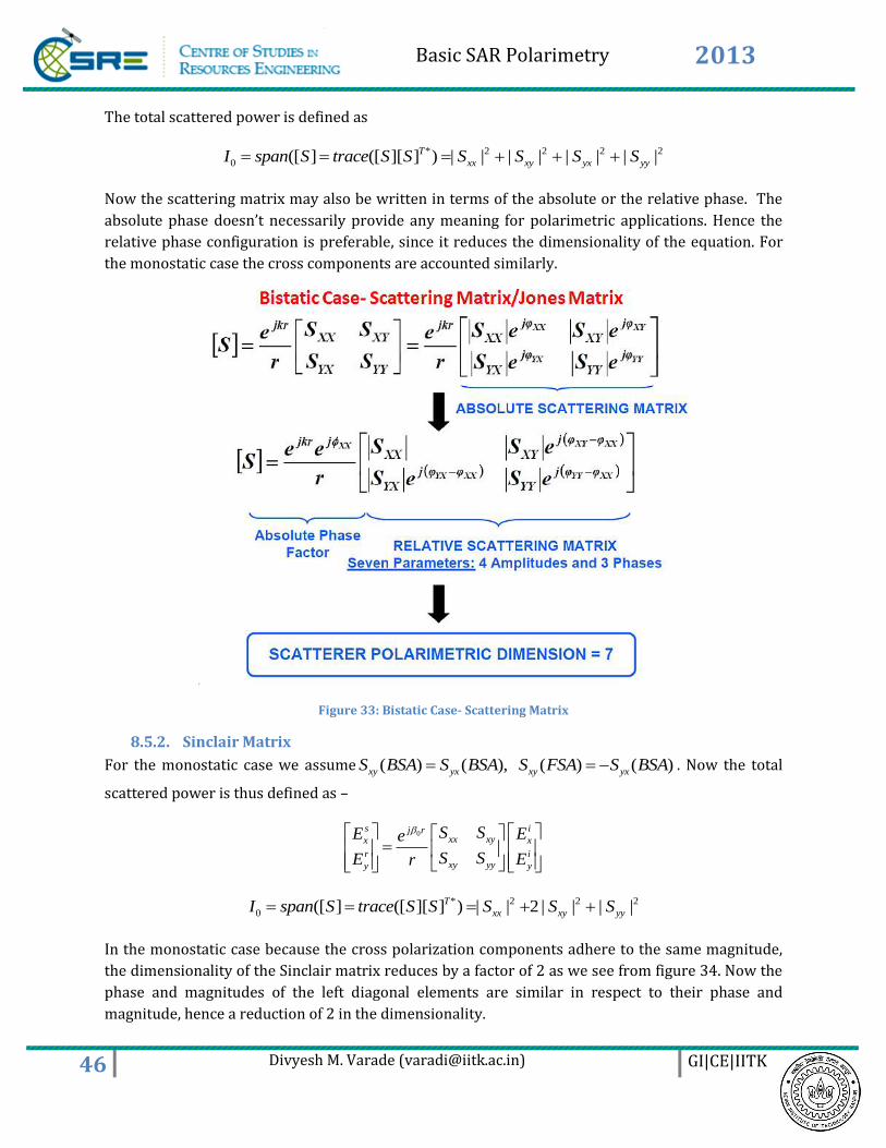
The total scattered power is defined as
* 2 2 2 2
0 ([ ] ([ ][ ] ) | | | | | | | |T
xx xy yx yyI span S trace S S S S S S
Now the scattering matrix may also be written in terms of the absolute or the relative phase. The
absolute phase doesn’t necessarily provide any meaning for polarimetric applications. Hence the
relative phase configuration is preferable, since it reduces the dimensionality of the equation. For
the monostatic case the cross components are accounted similarly.
Figure 33: Bistatic Case- Scattering Matrix
8.5.2. Sinclair Matrix
For the monostatic case we assume ( ) ( ), ( ) ( )xy yx xy yxS BSA S BSA S FSA S BSA . Now the total
scattered power is thus defined as –
0s ij r
xx xyx x
r ixy yyy y
S SE Ee
S SE Er
* 2 2 2
0 ([ ] ([ ][ ] ) | | 2 | | | |T
xx xy yyI span S trace S S S S S
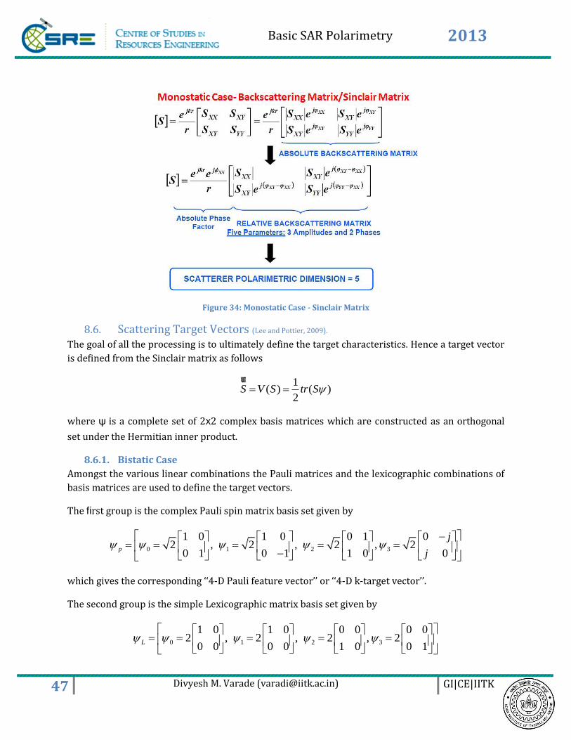
In the monostatic case because the cross polarization components adhere to the same magnitude,
the dimensionality of the Sinclair matrix reduces by a factor of 2 as we see from figure 34. Now the
phase and magnitudes of the left diagonal elements are similar in respect to their phase and
magnitude, hence a reduction of 2 in the dimensionality.
Basic SAR Polarimetry 2013
47 Divyesh M. Varade ([email protected]) GI|CE|IITK
Figure 34: Monostatic Case - Sinclair Matrix
8.6. Scattering Target Vectors (Lee and Pottier, 2009).
The goal of all the processing is to ultimately define the target characteristics. Hence a target vector
is defined from the Sinclair matrix as follows
1( ) ( )
2S V S tr S ur
where ψ is a complete set of 2x2 complex basis matrices which are constructed as an orthogonal
set under the Hermitian inner product.
8.6.1. Bistatic Case
Amongst the various linear combinations the Pauli matrices and the lexicographic combinations of
basis matrices are used to define the target vectors.
The first group is the complex Pauli spin matrix basis set given by
0 1 2 3
1 0 1 0 0 1 02 , 2 , 2 , 2
0 1 0 1 1 0 0p
j
j
which gives the corresponding ‘‘4-D Pauli feature vector’’ or ‘‘4-D k-target vector’’.
The second group is the simple Lexicographic matrix basis set given by
0 1 2 3
1 0 1 0 0 0 0 02 , 2 , 2 , 2
0 0 0 0 1 0 0 1L
Basic SAR Polarimetry 2013
48 Divyesh M. Varade ([email protected]) GI|CE|IITK
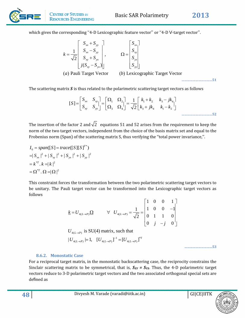
which gives the corresponding ‘‘4-D Lexicographic feature vector’’ or ‘‘4-D V-target vector’’.
1,
2
( )
( ) Pauli Target Vector ( ) Lexicographic Target Vector
xx yy xx
xx yy xy
xy yx yx
xy yx yy
S S S
S S Sk
S S S
j S S S
a b
……………………………51
The scattering matrix S is thus related to the polarimetric scattering target vectors as follows
1 2 1 2 3 4
3 4 3 4 1 2
1[ ]
2
xx xy
xy yy
S S k k k jkS
S S k jk k k
……………………………52
The insertion of the factor 2 and 2 equations 51 and 52 arises from the requirement to keep the
norm of the two target vectors, independent from the choice of the basis matrix set and equal to the
Frobenius norm (Span) of the scattering matrix S, thus verifying the ‘‘total power invariance,’’.
*
0
2 2 2 2
* 2
* 2
([ ] ([ ][ ] )
| | | | | | | |
. | |
. | |
T
xx xy yx yy
T
T
I span S trace S S
S S S S
k k k
This constraint forces the transformation between the two polarimetric scattering target vectors to
be unitary. The Pauli target vector can be transformed into the Lexicographic target vectors as
follows
4( ) 4( )
4( )
1 *
4( ) 4( ) 4( )
1 0 0 1
1 0 0 11
0 1 1 02
0 0
is SU(4) matrix, such that
| | 1, [ ] [ ]
L P L P
L P
T
L P L P L P
k U U
j j
U
U U U
…………………………53
8.6.2. Monostatic Case
For a reciprocal target matrix, in the monostatic backscattering case, the reciprocity constrains the
Sinclair scattering matrix to be symmetrical, that is, SXY = SYX. Thus, the 4-D polarimetric target
vectors reduce to 3-D polarimetric target vectors and the two associated orthogonal special sets are
defined as
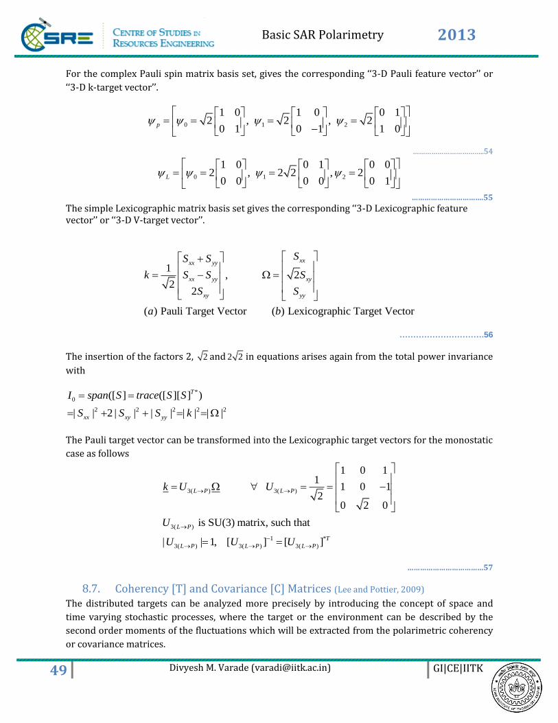
Basic SAR Polarimetry 2013
49 Divyesh M. Varade ([email protected]) GI|CE|IITK
For the complex Pauli spin matrix basis set, gives the corresponding ‘‘3-D Pauli feature vector’’ or
‘‘3-D k-target vector’’.
0 1 2
1 0 1 0 0 12 , 2 , 2
0 1 0 1 1 0p
……………………………..54
0 1 2
1 0 0 1 0 02 , 2 2 , 2
0 0 0 0 0 1L
…………………………….55
The simple Lexicographic matrix basis set gives the corresponding ‘‘3-D Lexicographic feature vector’’ or ‘‘3-D V-target vector’’.
1, 2
22
( ) Pauli Target Vector ( ) Lexicographic Target Vector
xxxx yy
xx yy xy
xy yy
SS S
k S S S
S S
a b
………………………….56
The insertion of the factors 2, 2 and 2 2 in equations arises again from the total power invariance
with
*
0
2 2 2 2 2
([ ] ([ ][ ] )
| | 2 | | | | | | | |
T
xx xy yy
I span S trace S S
S S S k
The Pauli target vector can be transformed into the Lexicographic target vectors for the monostatic
case as follows
3( ) 3( )
3( )
1 *
3( ) 3( ) 3( )
1 0 11
1 0 12
0 2 0
is SU(3) matrix, such that
| | 1, [ ] [ ]
L P L P
L P
T
L P L P L P
k U U
U
U U U
………………………………57
8.7. Coherency [T] and Covariance [C] Matrices (Lee and Pottier, 2009) The distributed targets can be analyzed more precisely by introducing the concept of space and
time varying stochastic processes, where the target or the environment can be described by the
second order moments of the fluctuations which will be extracted from the polarimetric coherency
or covariance matrices.
Basic SAR Polarimetry 2013
50 Divyesh M. Varade ([email protected]) GI|CE|IITK
8.7.1. Bistatic Case
The 4x4 polarimetric Pauli coherency T4 matrix and the 4x4 Lexicographic covariance C4 matrix are
generated from the outer product of the associated target vector with its conjugate transpose.
* *4 4 4 1 4 1 4 4 4 1 4 1. , . T T
x x x x x xT k k C
where temporal or spatial ensemble averaging is used assuming homogeneity of the random
medium.
2 * * *
1 1 2 1 3 1 4
* 2 * *
2 1 2 2 3 2 4
* * 2 *
3 1 3 2 3 3 4
* * * 2
4 1 4 2 4 3 4
1 2 3 4
*4 4 4 1 4 1
| |
| |,
| |
| |
1 1 1 1 [ ], [ ], [ ], [ ( )]
2 2 2 2
.
xx yy xx yy xy yx xy yx
Tx x x
k k k k k k k
k k k k k k k
k k k k k k k
k k k k k k k
k S S k S S k S S k j S S
T k k
…………………………..58
2 * * *
* 2 * *
* * 2 *
* * * 2
*4 4 4 1 4 1
| |
| |
| |
| |
.
XX XX XY XX YX XX YY
XY XX XY XY YX XY YY
YX XX YX XY YX YX YY
YY XX YY XY YY YX YY
Tx x x
S S S S S S S
S S S S S S S
S S S S S S S
S S S S S S S
C
…………………………..59
It is important to note that, by construction, the 4x4 polarimetric coherency T4 and covariance C4
matrices are both Hermitian positive semidefinite matrices which imply that they satisfy
tr(T4)=tr(C4)=Span and that they possess real nonnegative eigenvalues and orthogonal
eigenvectors.
The relation between the coherency T4 and covariance C4 matrices is given by
* *
4 4( ) 4( ) 4( )
* *
4( ) 4( )
* 1 1 *
4( ) 4( ) 4( ) 4( )
*1
4( ) 4 4( ) 4
. ( ) . ( )
.
. [ ] [ ]
.
T T
L P L P L P
T T
L P L P
T T
L P L P L P L P
T
L P L P
T k k U U k U
U U
U U U U
U C U C
Q
Q
Q
…………………………60
Basic SAR Polarimetry 2013
51 Divyesh M. Varade ([email protected]) GI|CE|IITK
From the T and C matrices we can observe that, [T] is associated to the physical and geometrical
properties of the scattering process while[C] is associated to the direct measurable parameters
from the sensor.
8.7.2. Monostatic Case
For a reciprocal target matrix, in the monostatic backscattering case, the reciprocity constrains the
Sinclair scattering matrix to be symmetrical, that is, SXY = SYX, thus, the 4-D polarimetric coherency
T4 and covariance C4 matrices reduce to 3-D polarimetric coherency T3 and covariance C3 matrices
as follows
2 * *
1 1 2 1 3
* 2 *
2 1 2 2 3
* * 2
3 1 3 2 3
1 2 3
2* *
2*
*3 3 3 1 3 1
3 3
| |
| | ,
| |
1 1 [ ], [ ], 2[( )]
2 2
[ ][ ] 2 [ ][ ]
[ ][ ] 2 [
.
xx yy xx yy xy
xx yy xx yy xx yy xx yy xy
xx yy xx yy xx yy xx
Tx x x
x
k k k k k
k k k k k
k k k k k
k S S k S S k S
S S S S S S S S S
S S S S S S S S
T k k
T
*
2* *
][ ]
2 [ ][ ] 2 [ ][ ] 4
yy xy
xy xx yy xy xx yy xy
S
S S S S S S S
……………………...61
2 * *
* * 2 *3 3 3 1 3 1
* * 2
2
2 2 2
2
| |
. | |
| |
XX XX XY XX YY
TXY XX XY YX YYx x x
YY XX YY XY YY
S S S S S
C S S S S S
S S S S S
………………………..62
The 3X3 polarimetric coherency T3 and covariance C3 matrices are also both Hermitian positive
semi definite matrices and are related together with
1
3 3( ) 3 3( )L P L PT U C U
8.8. Mueller [M] and Kennaugh [K] matrices (Lee and Pottier, 2009) The representation in terms of power allows evaluating the same physical event in different ways,
by considering mainly that this results from independent measurements. Suitable representations
of data in terms of power to describe backscattering mechanisms are more powerful. The most
important reason why power-related data are powerful is that the elimination of the absolute phase
from the target means that the power-related parameters become incoherently additive
parameters. The 4x4 Kennaugh K matrix is defined as follows
Basic SAR Polarimetry 2013
52 Divyesh M. Varade ([email protected]) GI|CE|IITK
1*.( *)K A S S A
where corresponds to the Kronecker tensori matrix product and increases the dimensionality of
the Scattering matrix for further decomposition into meaningful information.
1 0 0 1
* * 1 0 0 1* ,
* * 0 1 1 0
0 0
xx xy
yx yy
S S S SS S A
S S S S
j j
In the forward scattering case, this matrix is named the 4x4 Mueller [M] matrix.
8.8.1. Bistatic Case
The S matrix in this case is non symmetric. The S matrix can thus be splitted into a symmetric and a
skew symmetric component as
10 [ ]
2
10
2
S xy yxxx xy xx xy
Syx yy xy yy
xy yx
Sss S SS S S S
S Ss SssS S S S
Ss S S
The symmetric scattering Ss matrix models a monostatic configuration and the skewsymmetric
scattering SSS matrix models additional information resulting from the bistatic configuration. The
bistatic 4x4 Kennaugh matrix is then given by
1
0 0
0
0
0 0
*.( *)
0 0 0 0
0 0 0 0
0 0 0 0
0 0 0 0
K A S S A
K Ks Kc Kss
A B C H F I N L A
C A B E G I K M AK
H E A B D N K J A
E G D A B K M J A
0 0
0
0
0 0
A B A C I H N F L
C I A B A E K G MK
H N E K A B A D J
E K G M D J A B A
………………………………63
Basic SAR Polarimetry 2013
53 Divyesh M. Varade ([email protected]) GI|CE|IITK
2 2
0
2 2 2 2
0 0
2 *
0
*
1| | , | . |
4
1 1| | | . | , | | | . |
4 4
1| | , Im{ }
2
Re{ . ( )}
xx yy xy
xx yy xy xx yy xy
xx yy xx yy
xy xx yy
A S S A Sss S
B S S Ss S B S S Ss S
C B S S D S S
E Ss S S S
*
* *
2 2 *
* *
Im{ . ( )}
Im{ . ( )} Re{ . ( )}
1| | | | Im{ }
2
Re{ . ( )} Im{ . ( )}
Im{
xy xx yy
xy xx yy xy xx yy
yx xy yx xy
xy xx yy xy xx yy
F Ss S S S
G Ss S S S H Ss S S S
I S S J S S
K Sss S S S L Sss S S S
M
* *. ( )} Re{ . ( )}xy xx yy xy xx yySss S S S N Sss S S S
…………………………64
As the bistatic polarimetric dimension of the target is equal to seven, it is thus easy to conclude that
the 16 bistatic target parameters are related to each other by (16-7) = 9 equations that are called
the ‘‘bistatic target structure equations.’’ The associated bistatic coherency T4 matrix is then given
by
0
0
4
0
2
2
A C jD H jG L jK
C jD B B E jF M jNT
H jG E jF B B J jI
L jK M jN J jI A
………………………………….65
As the bistatic coherency T4 matrix is a rank 1, 4x4 Hermitian matrix, it follows that its 36 principal
minors are zero. From these 36 minor equations, nine equations can be extracted to define the
bistatic target structure equations
…………………………………66
Figure 34 shows the ‘‘bistatic target structure diagram’’ that is constructed in the same way as the
monostatic target structure diagram. This bistatic target structure diagram is extended from a
triangular surface (the monostatic target structure diagram) to a tetrahedral volume. The same
analysis can be conducted on this bistatic target structure diagram by associating the four bistatic
target generators (A0, B0+B, B0-B and A) with the six parameters pairs (E, F), (G, H), (I, J), (K, L), and
(M, N).
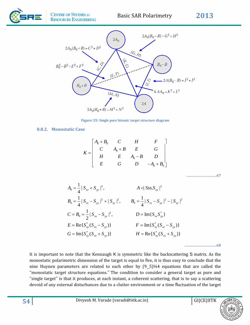
Basic SAR Polarimetry 2013
54 Divyesh M. Varade ([email protected]) GI|CE|IITK
Figure 35: Single pure bistatic target structure diagram
8.8.2. Monostatic Case
0 0
0
0
0 0
A B C H F
C A B E GK
H E A B D
E G D A B
…………………………..67
2 2
0
2 2 2 2
0 0
2 *
0
*
1| | , | . |
4
1 1| | | | , | | | |
4 4
1| | , Im{ }
2
Re{ ( )} Im{
xx yy xy
xx yy xy xx yy xy
xx yy xx yy
xy xx yy
A S S A Sss S
B S S S B S S S
C B S S D S S
E S S S F
*
* *
( )}
Im{ ( )} Re{ ( )}
xy xx yy
xy xx yy xy xx yy
S S S
G S S S H S S S
…………………………….68
It is important to note that the Kennaugh K is symmetric like the backscattering S matrix. As the
monostatic polarimetric dimension of the target is equal to five, it is thus easy to conclude that the
nine Huynen parameters are related to each other by (9_5)¼4 equations that are called the
‘‘monostatic target structure equations.’’ The condition to consider a general target as pure and
‘‘single target’’ is that it produces, at each instant, a coherent scattering, that is to say a scattering
devoid of any external disturbances due to a clutter environment or a time fluctuation of the target
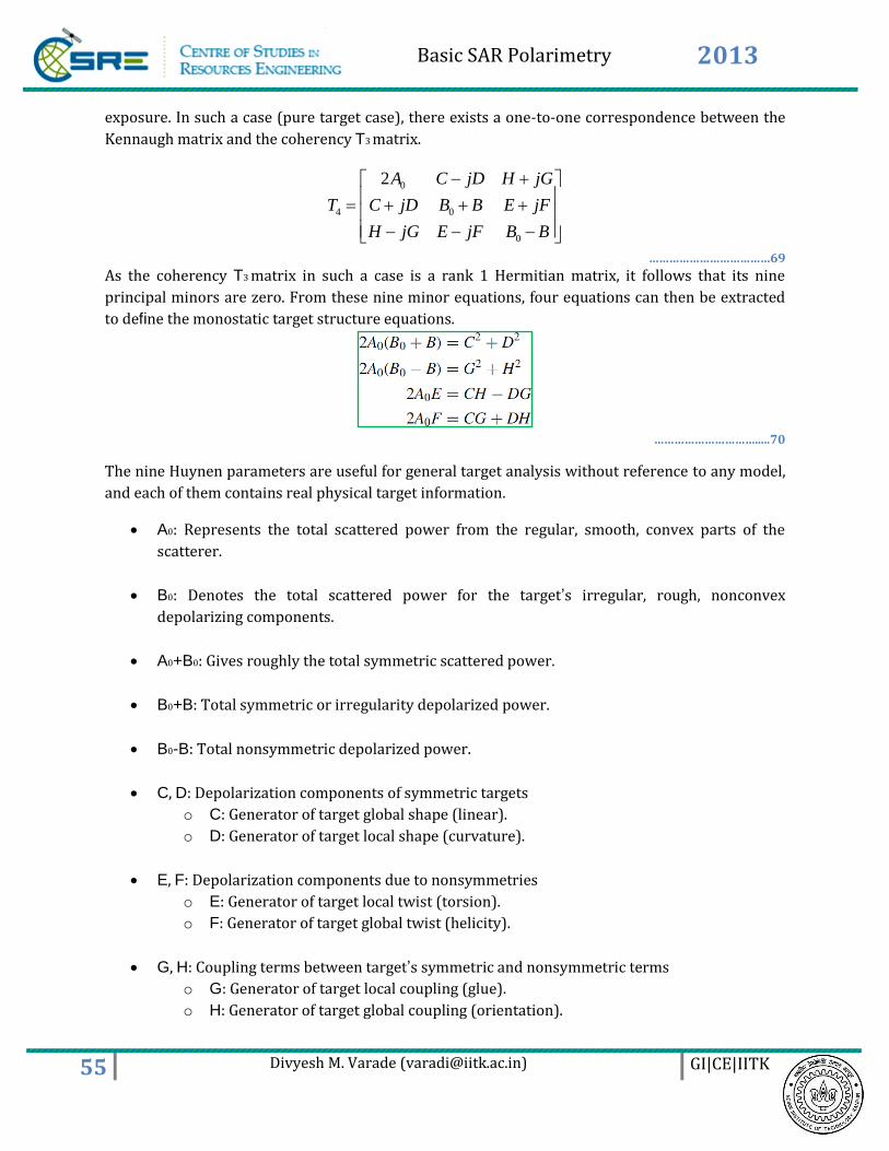
Basic SAR Polarimetry 2013
55 Divyesh M. Varade ([email protected]) GI|CE|IITK
exposure. In such a case (pure target case), there exists a one-to-one correspondence between the
Kennaugh matrix and the coherency T3 matrix.
0
4 0
0
2A C jD H jG
T C jD B B E jF
H jG E jF B B
………………………………69
As the coherency T3 matrix in such a case is a rank 1 Hermitian matrix, it follows that its nine
principal minors are zero. From these nine minor equations, four equations can then be extracted
to define the monostatic target structure equations.
………………………….....70
The nine Huynen parameters are useful for general target analysis without reference to any model,
and each of them contains real physical target information.
A0: Represents the total scattered power from the regular, smooth, convex parts of the
scatterer.
B0: Denotes the total scattered power for the target’s irregular, rough, nonconvex
depolarizing components.
A0+B0: Gives roughly the total symmetric scattered power.
B0+B: Total symmetric or irregularity depolarized power.
B0-B: Total nonsymmetric depolarized power.
C, D: Depolarization components of symmetric targets
o C: Generator of target global shape (linear).
o D: Generator of target local shape (curvature).
E, F: Depolarization components due to nonsymmetries
o E: Generator of target local twist (torsion).
o F: Generator of target global twist (helicity).
G, H: Coupling terms between target’s symmetric and nonsymmetric terms
o G: Generator of target local coupling (glue).
o H: Generator of target global coupling (orientation).
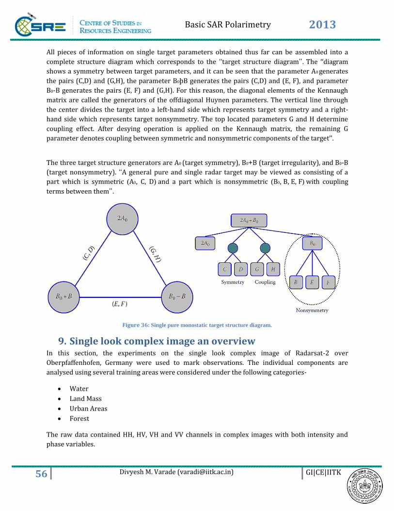
Basic SAR Polarimetry 2013
56 Divyesh M. Varade ([email protected]) GI|CE|IITK
All pieces of information on single target parameters obtained thus far can be assembled into a
complete structure diagram which corresponds to the ‘‘target structure diagram’’. The ‘‘diagram
shows a symmetry between target parameters, and it can be seen that the parameter A0 generates
the pairs (C,D) and (G,H), the parameter B0þB generates the pairs (C,D) and (E, F), and parameter
B0-B generates the pairs (E, F) and (G,H). For this reason, the diagonal elements of the Kennaugh
matrix are called the generators of the offdiagonal Huynen parameters. The vertical line through
the center divides the target into a left-hand side which represents target symmetry and a right-
hand side which represents target nonsymmetry. The top located parameters G and H determine
coupling effect. After desying operation is applied on the Kennaugh matrix, the remaining G
parameter denotes coupling between symmetric and nonsymmetric components of the target’’.
The three target structure generators are A0 (target symmetry), B0+B (target irregularity), and B0-B
(target nonsymmetry). ‘‘A general pure and single radar target may be viewed as consisting of a
part which is symmetric (A0, C, D) and a part which is nonsymmetric (B0, B, E, F) with coupling
terms between them’’.
Figure 36: Single pure monostatic target structure diagram.
9. Single look complex image an overview In this section, the experiments on the single look complex image of Radarsat-2 over
Oberpfaffenhofen, Germany were used to mark observations. The individual components are
analysed using several training areas were considered under the following categories-
Water
Land Mass
Urban Areas
Forest
The raw data contained HH, HV, VH and VV channels in complex images with both intensity and
phase variables.
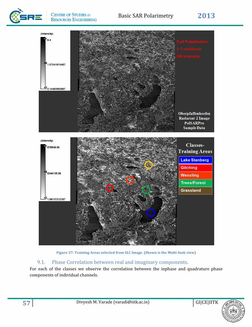
Basic SAR Polarimetry 2013
57 Divyesh M. Varade ([email protected]) GI|CE|IITK
Figure 37: Training Areas selected from SLC Image. (Shown is the Multi-look view)
9.1. Phase Correlation between real and imaginary components. For each of the classes we observe the correlation between the inphase and quadrature phase
components of individual channels.
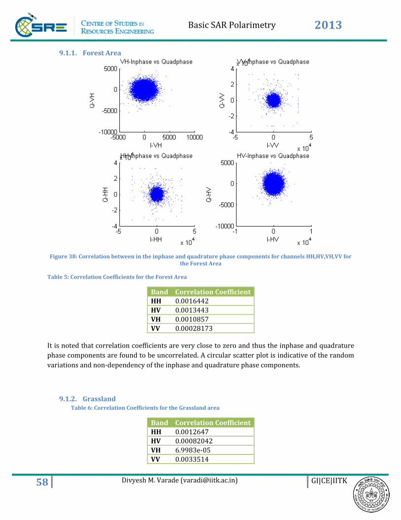
Basic SAR Polarimetry 2013
58 Divyesh M. Varade ([email protected]) GI|CE|IITK
9.1.1. Forest Area
Figure 38: Correlation between in the inphase and quadrature phase components for channels HH,HV,VH,VV for the Forest Area
Table 5: Correlation Coefficients for the Forest Area
Band Correlation Coefficient HH 0.0016442
HV 0.0013443
VH 0.0010857
VV 0.00028173
It is noted that correlation coefficients are very close to zero and thus the inphase and quadrature
phase components are found to be uncorrelated. A circular scatter plot is indicative of the random
variations and non-dependency of the inphase and quadrature phase components.
9.1.2. Grassland Table 6: Correlation Coefficients for the Grassland area
Band Correlation Coefficient
HH 0.0012647 HV 0.00082042 VH 6.9983e-05 VV 0.0033514
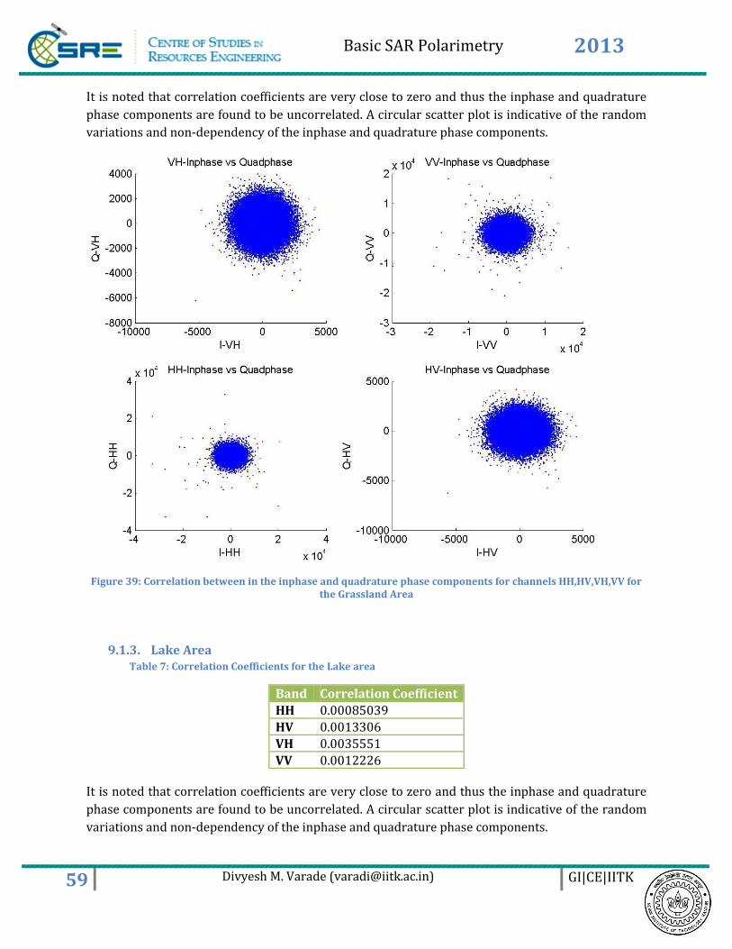
Basic SAR Polarimetry 2013
59 Divyesh M. Varade ([email protected]) GI|CE|IITK
It is noted that correlation coefficients are very close to zero and thus the inphase and quadrature
phase components are found to be uncorrelated. A circular scatter plot is indicative of the random
variations and non-dependency of the inphase and quadrature phase components.
Figure 39: Correlation between in the inphase and quadrature phase components for channels HH,HV,VH,VV for the Grassland Area
9.1.3. Lake Area Table 7: Correlation Coefficients for the Lake area
Band Correlation Coefficient
HH 0.00085039 HV 0.0013306 VH 0.0035551 VV 0.0012226
It is noted that correlation coefficients are very close to zero and thus the inphase and quadrature
phase components are found to be uncorrelated. A circular scatter plot is indicative of the random
variations and non-dependency of the inphase and quadrature phase components.
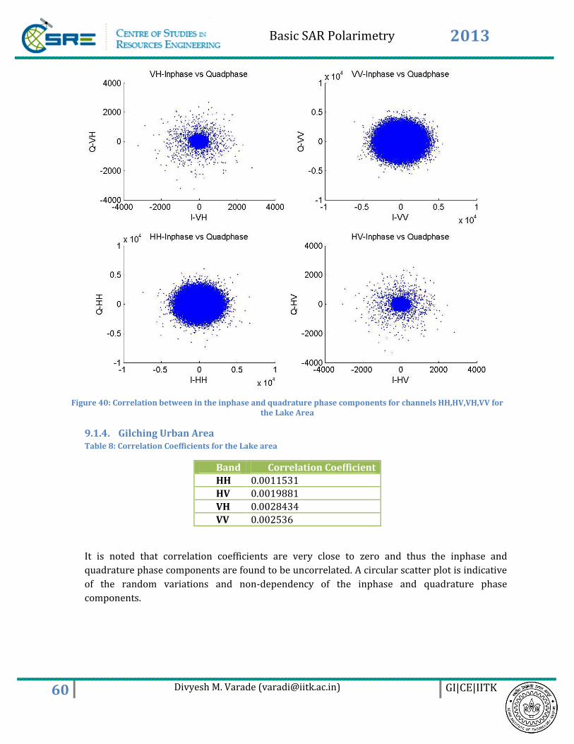
Basic SAR Polarimetry 2013
60 Divyesh M. Varade ([email protected]) GI|CE|IITK
Figure 40: Correlation between in the inphase and quadrature phase components for channels HH,HV,VH,VV for the Lake Area
9.1.4. Gilching Urban Area Table 8: Correlation Coefficients for the Lake area
Band Correlation Coefficient HH 0.0011531 HV 0.0019881 VH 0.0028434 VV 0.002536
It is noted that correlation coefficients are very close to zero and thus the inphase and
quadrature phase components are found to be uncorrelated. A circular scatter plot is indicative
of the random variations and non-dependency of the inphase and quadrature phase
components.
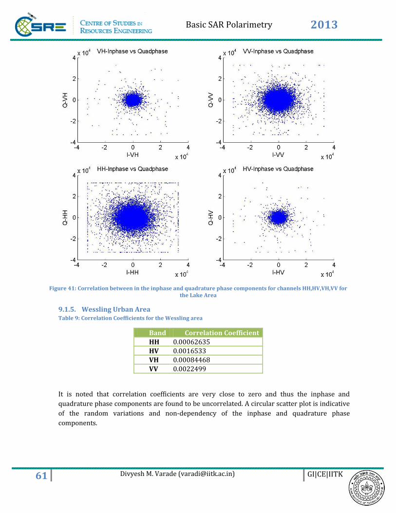
Basic SAR Polarimetry 2013
61 Divyesh M. Varade ([email protected]) GI|CE|IITK
Figure 41: Correlation between in the inphase and quadrature phase components for channels HH,HV,VH,VV for the Lake Area
9.1.5. Wessling Urban Area Table 9: Correlation Coefficients for the Wessling area
Band Correlation Coefficient
HH 0.00062635 HV 0.0016533 VH 0.00084468 VV 0.0022499
It is noted that correlation coefficients are very close to zero and thus the inphase and
quadrature phase components are found to be uncorrelated. A circular scatter plot is indicative
of the random variations and non-dependency of the inphase and quadrature phase
components.
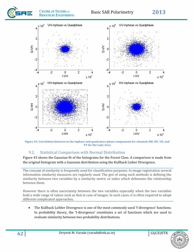
Basic SAR Polarimetry 2013
62 Divyesh M. Varade ([email protected]) GI|CE|IITK
Figure 42: Correlation between in the inphase and quadrature phase components for channels HH, HV, VH, and VV for the Lake Area
9.2. Statistical Comparison with Normal Distribution Figure 43 shows the Gaussian fit of the histograms for the Forest Class. A comparison is made from
the original histogram with a Gaussian distribution using the Kullback Lieber Divergence.
The concept of similarity is frequently used for classification purposes. In image registration several information similarity measures are regularly used. The gist of using such methods is defining the similarity between two variables by a similarity metric or index which delineates the relationship between them. However there is often uncertainty between the two variables especially when the two variables hold a wide range of values such as that in case of images. In such cases, it is often required to adopt different complicated approaches.
The Kullback Leibler Divergence is one of the most commonly used ‘f-divergence’ functions.
In probability theory, the ‘f-divergence’ constitutes a set of functions which are used to
evaluate similarity between two probability distributions.
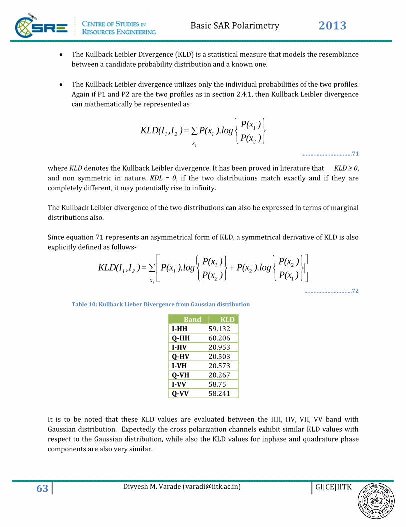
Basic SAR Polarimetry 2013
63 Divyesh M. Varade ([email protected]) GI|CE|IITK
The Kullback Leibler Divergence (KLD) is a statistical measure that models the resemblance
between a candidate probability distribution and a known one.
The Kullback Leibler divergence utilizes only the individual probabilities of the two profiles.
Again if P1 and P2 are the two profiles as in section 2.4.1, then Kullback Leibler divergence
can mathematically be represented as
1
11 2 1
2x
P(x )KLD(I ,I )= P(x ).log
P(x )
……………………………71
where KLD denotes the Kullback Leibler divergence. It has been proved in literature that KLD ≥ 0,
and non symmetric in nature. KDL = 0, if the two distributions match exactly and if they are
completely different, it may potentially rise to infinity.
The Kullback Leibler divergence of the two distributions can also be expressed in terms of marginal
distributions also.
Since equation 71 represents an asymmetrical form of KLD, a symmetrical derivative of KLD is also
explicitly defined as follows-
22
11
11 2 1
2x
P(x ) P(x )KLD(I ,I )= P(x ).log P(x ).log
P(x ) P(x )
………………………….72
Table 10: Kullback Lieber Divergence from Gaussian distribution
Band KLD
I-HH 59.132 Q-HH 60.206 I-HV 20.953 Q-HV 20.503 I-VH 20.573 Q-VH 20.267 I-VV 58.75 Q-VV 58.241
It is to be noted that these KLD values are evaluated between the HH, HV, VH, VV band with
Gaussian distribution. Expectedly the cross polarization channels exhibit similar KLD values with
respect to the Gaussian distribution, while also the KLD values for inphase and quadrature phase
components are also very similar.
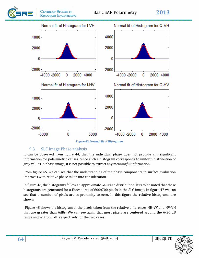
Basic SAR Polarimetry 2013
64 Divyesh M. Varade ([email protected]) GI|CE|IITK
Figure 43: Normal fit of Histograms
9.3. SLC Image Phase analysis It can be observed from figure 44, that the individual phase does not provide any significant
information for polarimetric causes. Since such a histogram corresponds to uniform distribution of
gray values in phase image, it is not possible to extract any meaningful information.
From figure 45, we can see that the understanding of the phase components in surface evaluation
improves with relative phase taken into consideration.
In figure 46, the histograms follow an approximate Gaussian distribution. It is to be noted that these
histograms are generated for a Forest area of 600x700 pixels in the SLC image. In figure 47 we can
see that a number of pixels are in proximity to zero. In this figure the relative histograms are
shown.
Figure 48 shows the histogram of the pixels taken from the relative differences HH-VV and HV-VH
that are greater than 6dBs. We can see again that most pixels are centered around the 6-20 dB
range and -20 to 20 dB respectively for the two cases.
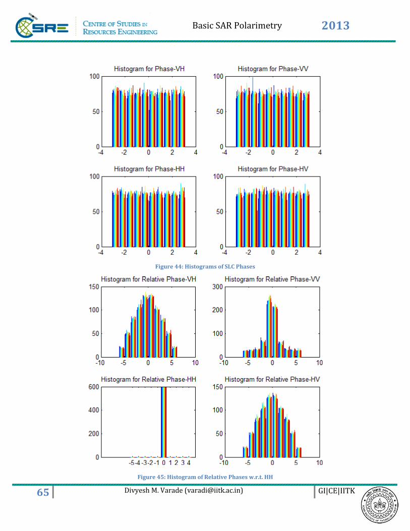
Basic SAR Polarimetry 2013
65 Divyesh M. Varade ([email protected]) GI|CE|IITK
Figure 44: Histograms of SLC Phases
Figure 45: Histogram of Relative Phases w.r.t. HH
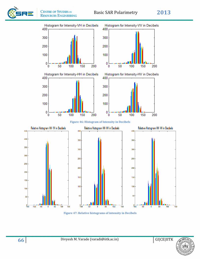
Basic SAR Polarimetry 2013
66 Divyesh M. Varade ([email protected]) GI|CE|IITK
Figure 46: Histogram of Intensity in Decibels
Figure 47: Relative histograms of intensity in Decibels
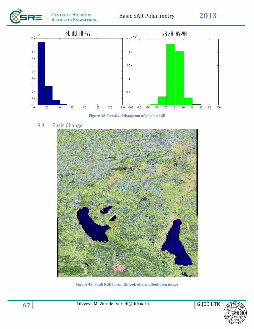
Basic SAR Polarimetry 2013
67 Divyesh M. Varade ([email protected]) GI|CE|IITK
Figure 48: Relative Histogram of pixels >6dB
9.4. Basis Change
Figure 49: Pauli RGB for multi-look oberpfaffenhofen image
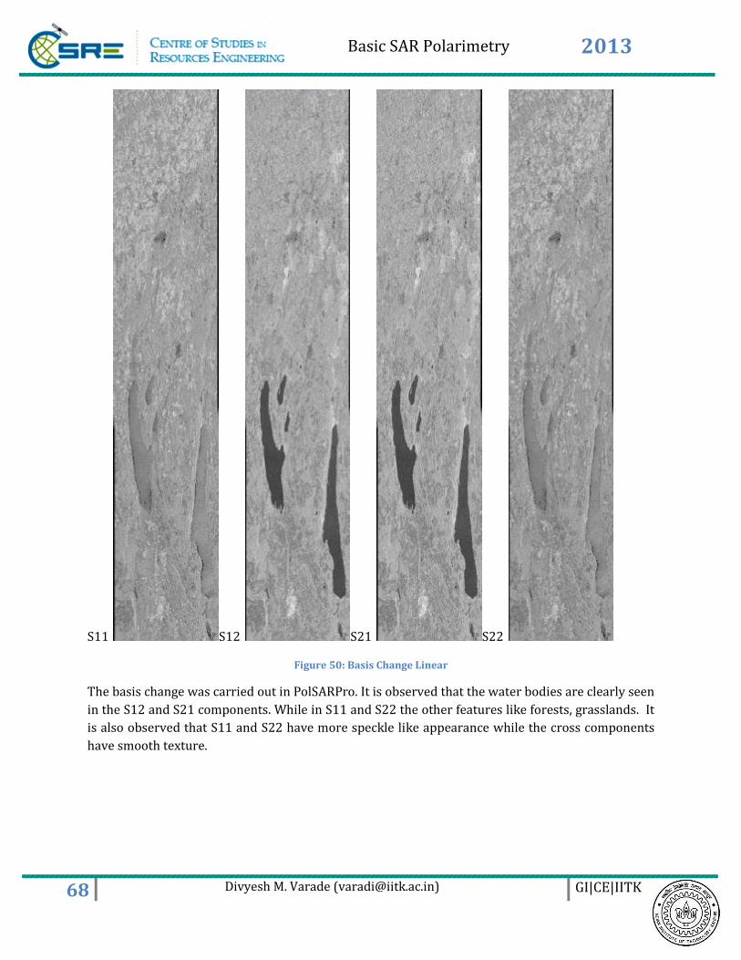
Basic SAR Polarimetry 2013
68 Divyesh M. Varade ([email protected]) GI|CE|IITK
S11 S12 S21 S22
Figure 50: Basis Change Linear
The basis change was carried out in PolSARPro. It is observed that the water bodies are clearly seen
in the S12 and S21 components. While in S11 and S22 the other features like forests, grasslands. It
is also observed that S11 and S22 have more speckle like appearance while the cross components
have smooth texture.
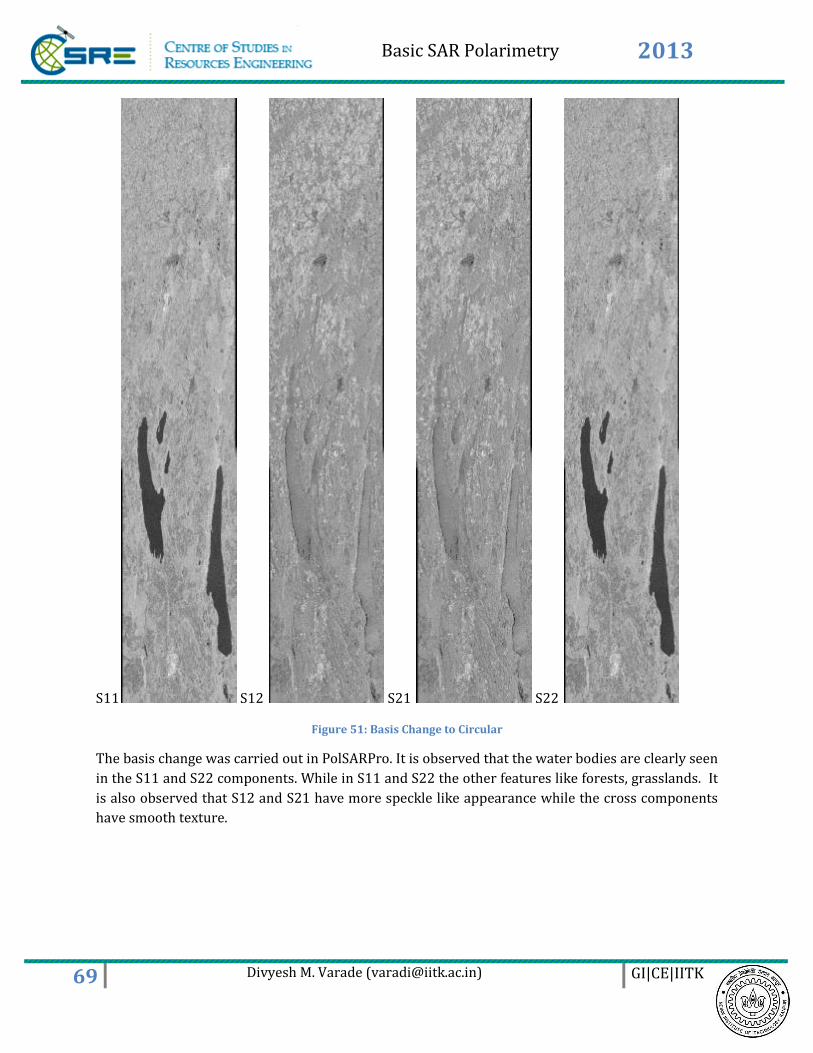
Basic SAR Polarimetry 2013
69 Divyesh M. Varade ([email protected]) GI|CE|IITK
S11 S12 S21 S22
Figure 51: Basis Change to Circular
The basis change was carried out in PolSARPro. It is observed that the water bodies are clearly seen
in the S11 and S22 components. While in S11 and S22 the other features like forests, grasslands. It
is also observed that S12 and S21 have more speckle like appearance while the cross components
have smooth texture.
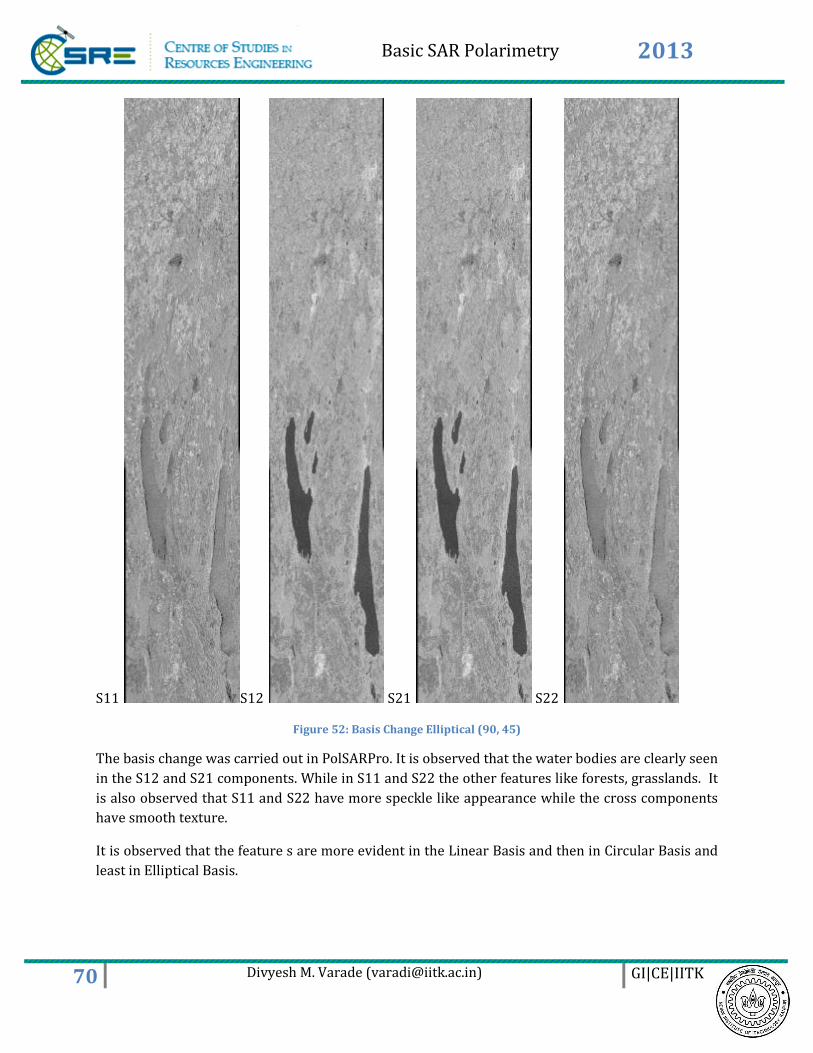
Basic SAR Polarimetry 2013
70 Divyesh M. Varade ([email protected]) GI|CE|IITK
S11 S12 S21 S22
Figure 52: Basis Change Elliptical (90, 45)
The basis change was carried out in PolSARPro. It is observed that the water bodies are clearly seen
in the S12 and S21 components. While in S11 and S22 the other features like forests, grasslands. It
is also observed that S11 and S22 have more speckle like appearance while the cross components
have smooth texture.
It is observed that the feature s are more evident in the Linear Basis and then in Circular Basis and
least in Elliptical Basis.
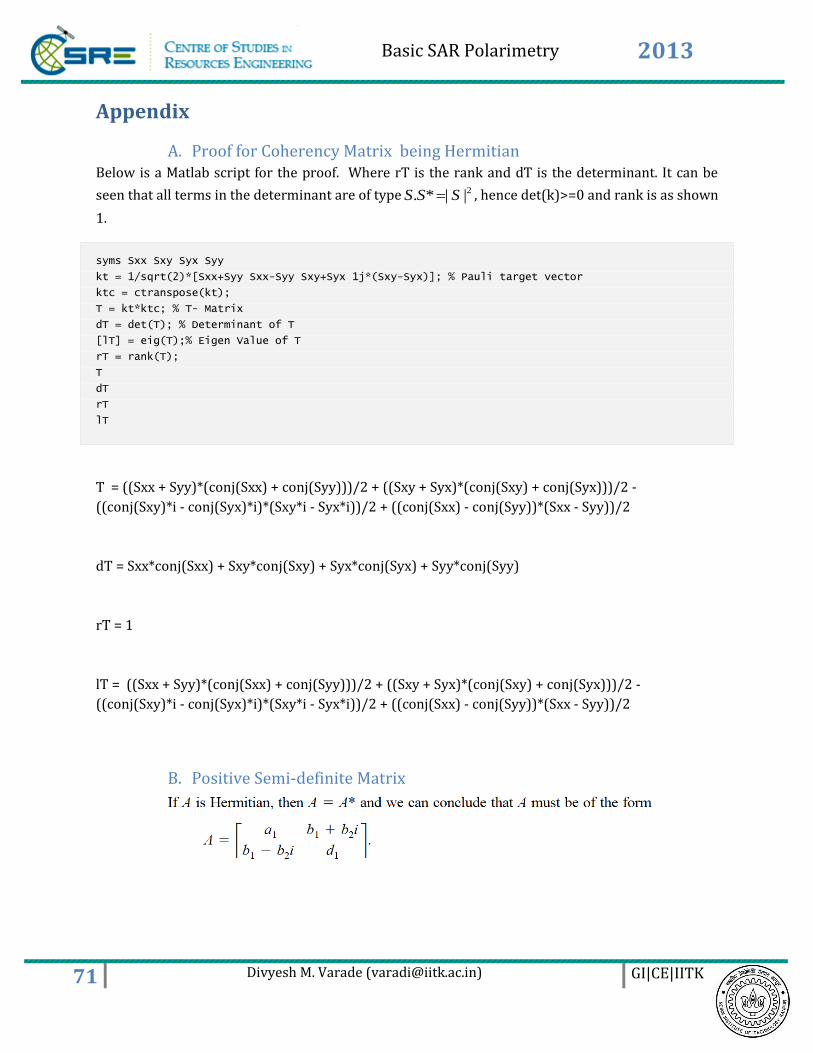
Basic SAR Polarimetry 2013
71 Divyesh M. Varade ([email protected]) GI|CE|IITK
Appendix
A. Proof for Coherency Matrix being Hermitian Below is a Matlab script for the proof. Where rT is the rank and dT is the determinant. It can be
seen that all terms in the determinant are of type 2. * | |S S S , hence det(k)>=0 and rank is as shown
1.
syms Sxx Sxy Syx Syy
kt = 1/sqrt(2)*[Sxx+Syy Sxx-Syy Sxy+Syx 1j*(Sxy-Syx)]; % Pauli target vector
ktc = ctranspose(kt);
T = kt*ktc; % T- Matrix
dT = det(T); % Determinant of T
[lT] = eig(T);% Eigen Value of T
rT = rank(T);
T
dT
rT
lT
T = ((Sxx + Syy)*(conj(Sxx) + conj(Syy)))/2 + ((Sxy + Syx)*(conj(Sxy) + conj(Syx)))/2 -
((conj(Sxy)*i - conj(Syx)*i)*(Sxy*i - Syx*i))/2 + ((conj(Sxx) - conj(Syy))*(Sxx - Syy))/2
dT = Sxx*conj(Sxx) + Sxy*conj(Sxy) + Syx*conj(Syx) + Syy*conj(Syy)
rT = 1
lT = ((Sxx + Syy)*(conj(Sxx) + conj(Syy)))/2 + ((Sxy + Syx)*(conj(Sxy) + conj(Syx)))/2 -
((conj(Sxy)*i - conj(Syx)*i)*(Sxy*i - Syx*i))/2 + ((conj(Sxx) - conj(Syy))*(Sxx - Syy))/2
B. Positive Semi-definite Matrix
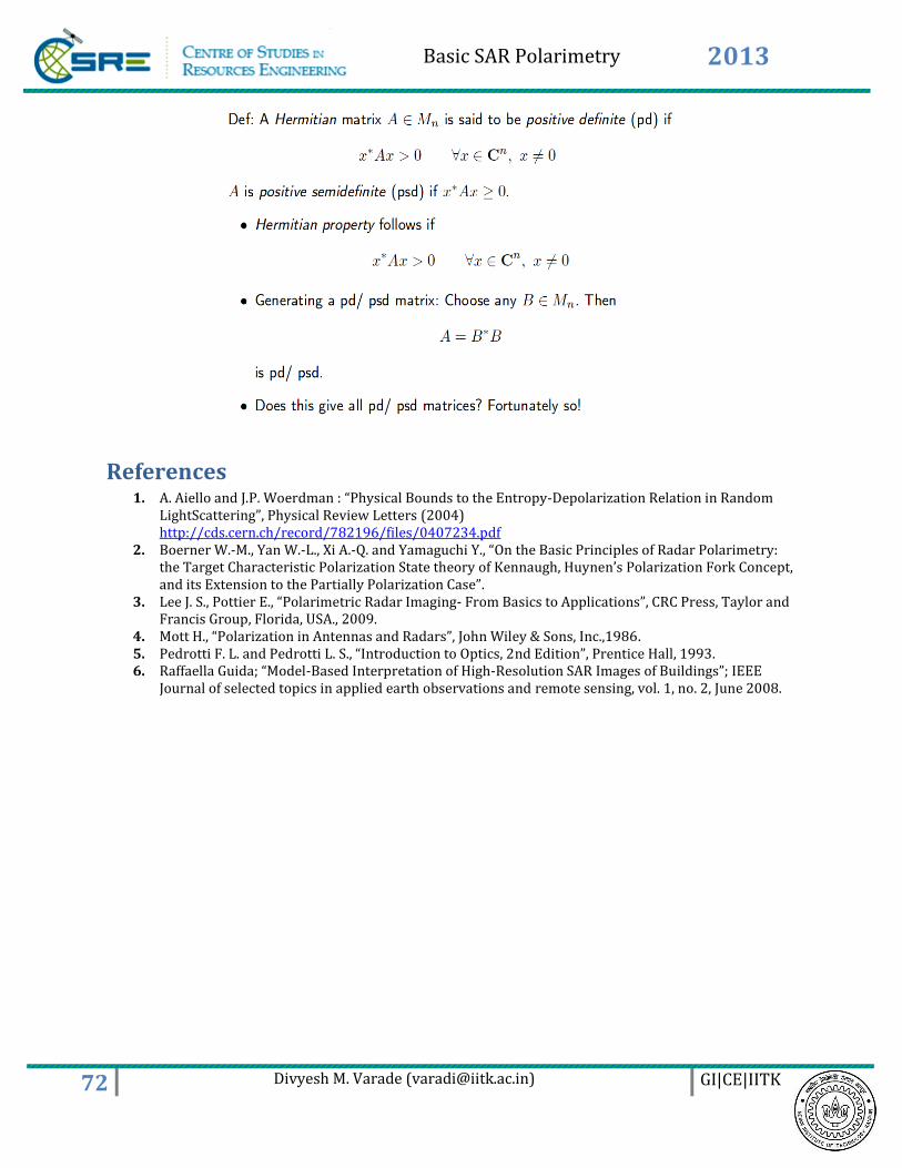
Basic SAR Polarimetry 2013
72 Divyesh M. Varade ([email protected]) GI|CE|IITK
References 1. A. Aiello and J.P. Woerdman : “Physical Bounds to the Entropy-Depolarization Relation in Random
LightScattering”, Physical Review Letters (2004) http://cds.cern.ch/record/782196/files/0407234.pdf
2. Boerner W.-M., Yan W.-L., Xi A.-Q. and Yamaguchi Y., “On the Basic Principles of Radar Polarimetry: the Target Characteristic Polarization State theory of Kennaugh, Huynen’s Polarization Fork Concept, and its Extension to the Partially Polarization Case”.
3. Lee J. S., Pottier E., “Polarimetric Radar Imaging- From Basics to Applications”, CRC Press, Taylor and Francis Group, Florida, USA., 2009.
4. Mott H., “Polarization in Antennas and Radars”, John Wiley & Sons, Inc.,1986. 5. Pedrotti F. L. and Pedrotti L. S., “Introduction to Optics, 2nd Edition”, Prentice Hall, 1993. 6. Raffaella Guida; “Model-Based Interpretation of High-Resolution SAR Images of Buildings”; IEEE
Journal of selected topics in applied earth observations and remote sensing, vol. 1, no. 2, June 2008.