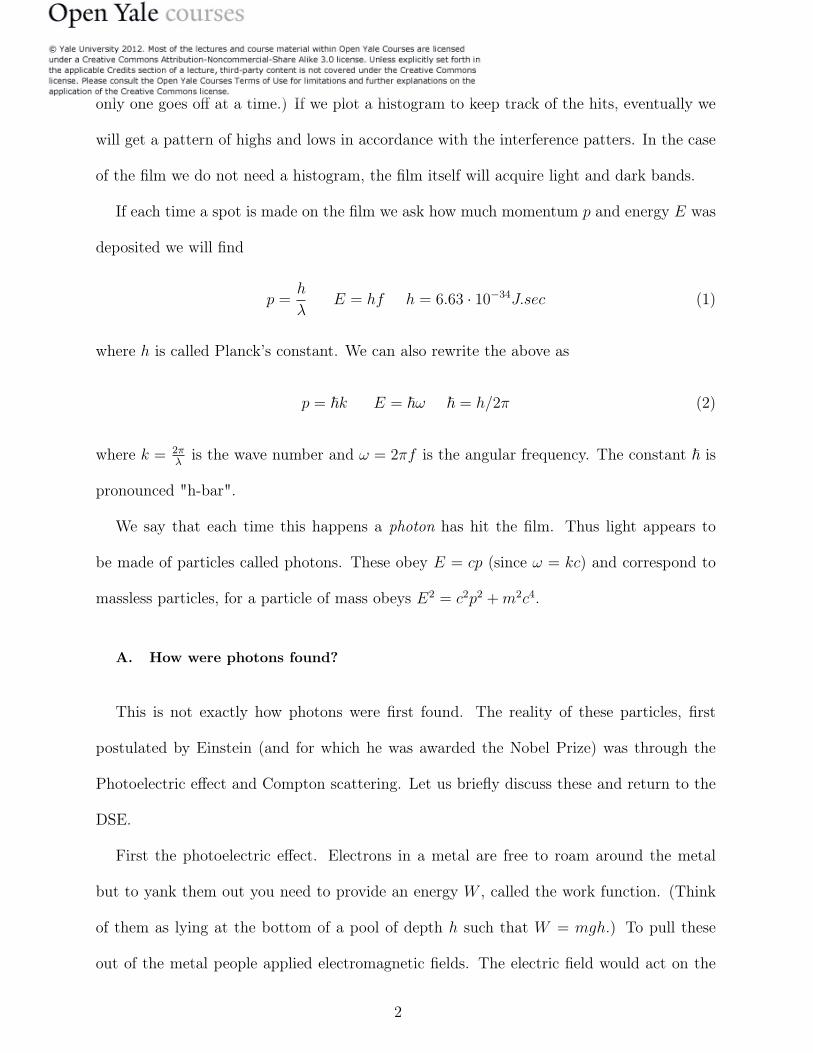
PHYSICS 201b Quantum notes R. Shankar 2010

These notes, possibly containing some bugs were for students of Physics 201b.

They may not be reproduced for commercial purposes.

I. THE DOUBLE SLIT EXPERIMENT

I am going to begin with the double slit experiment (DSE).

Consider the experiment with light. It has been known from Young’s double slit exper-

iment that light is a wave since it exhibits an interference pattern. Maxwell’s theory also

describes light as electromagnetic waves.

Consider a DSE with light of wavelength λ. Assume we are seeing a robust interference

pattern. The light detector behind the double slit could be a photographic plate or film

which shows dark and light bands when exposed for some time to this light.The brightness

at some point is given by the intensity I = A2, where A is the amplitude. The incoming

beam has a fixed amplitude before interference. After interference, on a screen where the

light falls, the amplitude A varies as we move up and down the screen parallel to the slits.

Suppose we now keep on reducing the brightness or intensity of the incoming beam. We

expect that the interference pattern will keep getting dimmer on the film and that it will

take longer and longer to get the desired exposure for us to see the pattern clearly. However

we expect the entire film to receive the light beam. If the light hitting the film is like a wave

hitting the beach, we expect that as we reduce the intensity, the height of the wave will keep

dropping, but it will hit the entire beach.

What happens is however different. In the extreme case it will look like this. We slip in

a new plate and wait. We find nothing happens for a while and suddenly one spot on the

film gets hit. After a while another spot gets hit. (If we had an array of light detectors,

1

only one goes off at a time.) If we plot a histogram to keep track of the hits, eventually we

will get a pattern of highs and lows in accordance with the interference patters. In the case

of the film we do not need a histogram, the film itself will acquire light and dark bands.

If each time a spot is made on the film we ask how much momentum p and energy E was

deposited we will find

p =h

λE = hf h = 6.63 · 10−34

J.sec (1)

where h is called Planck’s constant. We can also rewrite the above as

p = �k E = �ω � = h/2π (2)

where k = 2πλ is the wave number and ω = 2πf is the angular frequency. The constant � is

pronounced "h-bar".

We say that each time this happens a photon has hit the film. Thus light appears to

be made of particles called photons. These obey E = cp (since ω = kc) and correspond to

massless particles, for a particle of mass obeys E2 = c

2p

2 + m2c4.

A. How were photons found?

This is not exactly how photons were first found. The reality of these particles, first

postulated by Einstein (and for which he was awarded the Nobel Prize) was through the

Photoelectric effect and Compton scattering. Let us briefly discuss these and return to the

DSE.

First the photoelectric effect. Electrons in a metal are free to roam around the metal

but to yank them out you need to provide an energy W , called the work function. (Think

of them as lying at the bottom of a pool of depth h such that W = mgh.) To pull these

out of the metal people applied electromagnetic fields. The electric field would act on the

2

K

W ωh

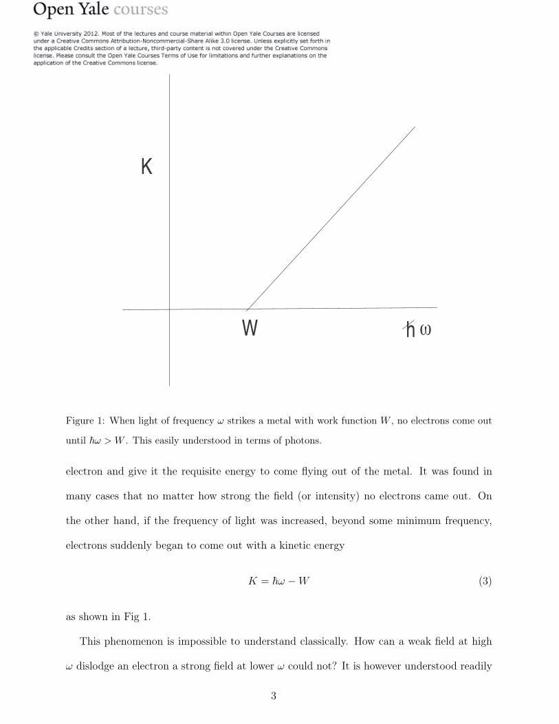
Figure 1: When light of frequency ω strikes a metal with work function W , no electrons come out

until �ω > W . This easily understood in terms of photons.

electron and give it the requisite energy to come flying out of the metal. It was found in

many cases that no matter how strong the field (or intensity) no electrons came out. On

the other hand, if the frequency of light was increased, beyond some minimum frequency,

electrons suddenly began to come out with a kinetic energy

K = �ω −W (3)

as shown in Fig 1.

This phenomenon is impossible to understand classically. How can a weak field at high

ω dislodge an electron a strong field at lower ω could not? It is however understood readily

3

if the beam is viewed in terms of photons. A strong beam at low frequency indeed sends

many many photons, each with energy that is too low to free the electron, while a weak field

at high ω sends fewer photons, but each with enough energy to get the job done (free the

electron). (Why don’t many of the numerous weak photons join forces and yank the electron

out? The probability for this "multi-photon event" happens to be to be very small.)

Now for the Compton Effect. When light of wavelength λ bounces off a static electron,

it is found that its wavelength gets altered:

δλ =2π�mc

(1− cos θ) (4)

where θ is the angle between incident and final beams. If you treat the collision as between

the electron and photons of energy and momentum given by Eqn. (1) following relativistic

kinematics you will find (or rather, you found last term) the above result.

Back to the double slit. Is light a particle or wave? It is certainly particle-like in that

the detector is hit by one photon at a time, each of which carries a definite momentum and

energy and dumps all of it at one point. The wavelength and frequency are not evident here

except in the energy and momentum they carry. If however the experiment is allowed to

continue till many many photons have arrived we see an interference pattern appropriate to

the λ in question.

In other words, photons are particles, but their arrival rate at the screen or detector is

controlled by a wave. The wave is not physical and is associated with each photon. It

determines the odds that the photon will arrive at some point on the screen. When we

send a macroscopic beam of light with zillions of photons, the interference patters seems to

come on instantaneously when in fact it is built dot by dot, with the odds for each being

determined by the interference pattern- the odds are high at bright regions, low at dark

regions. The wave is called the wave function. More on this later.

4

B. Enter de Broglie

de Broglie said this " If light, which we thought was surely a wave has particle properties

(made up of photons), then things like electrons, which we were sure were particles, must

have wave like properties. I postulate that with every electron of momentum p there is an

associated wave with wavelength

λ =2π�p

("de Broglie relation") (5)

Sure enough, when a double slit experiment was done with electrons of momentum p, an

interference pattern with this λ was seen, with more electrons coming where the interfer-

ence was constructive and less where it was destructive and zero where there was complete

cancellation.

With light, the interference pattern was not a shock, the discrete bundles of energy and

momentum, the photons, were. Here the particles (electrons) hitting the detector or back

screen at isolated points was expected, but the interference pattern was not.

Let us make sure we understand the implications of the double slit experiment was done

with electrons. Consider Fig. ??.

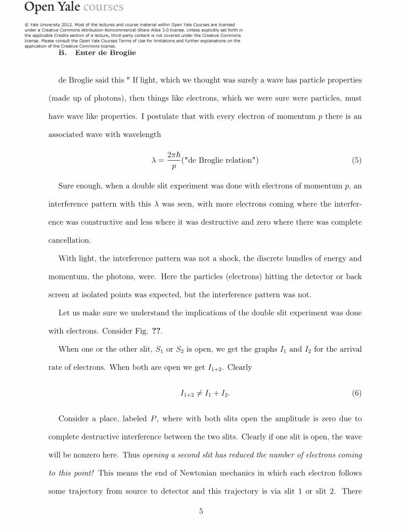
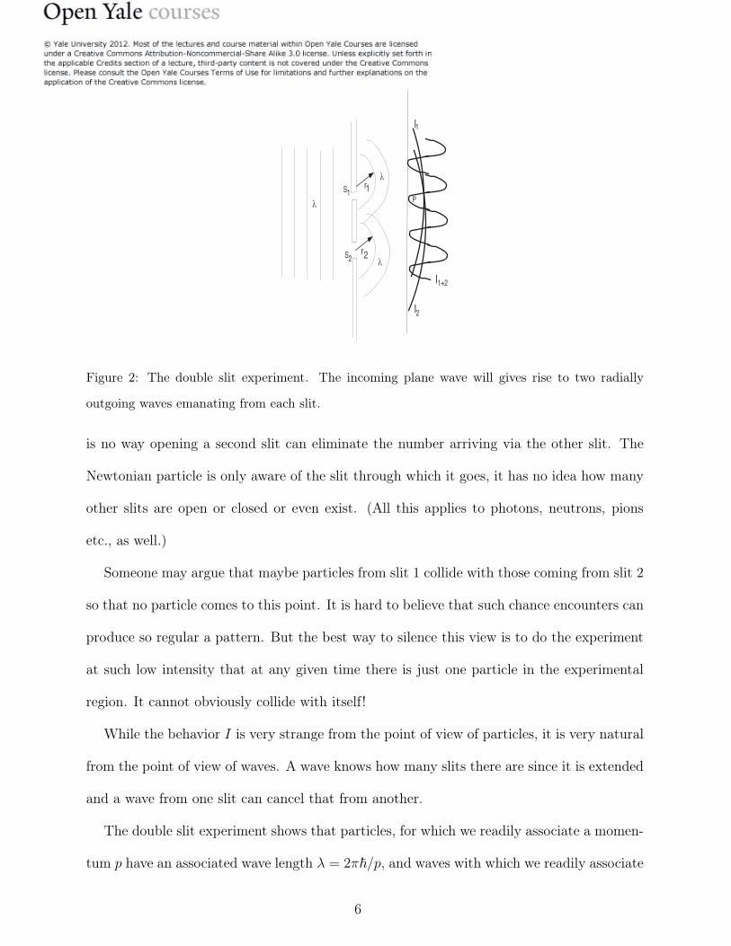
When one or the other slit, S1 or S2 is open, we get the graphs I1 and I2 for the arrival

rate of electrons. When both are open we get I1+2. Clearly

I1+2 �= I1 + I2. (6)

Consider a place, labeled P , where with both slits open the amplitude is zero due to

complete destructive interference between the two slits. Clearly if one slit is open, the wave

will be nonzero here. Thus opening a second slit has reduced the number of electrons coming

to this point! This means the end of Newtonian mechanics in which each electron follows

some trajectory from source to detector and this trajectory is via slit 1 or slit 2. There

5

r

r1

2

λ

λ

λ

I

I2

I1

1+2

S

S

1

2

P

Figure 2: The double slit experiment. The incoming plane wave will gives rise to two radially

outgoing waves emanating from each slit.

is no way opening a second slit can eliminate the number arriving via the other slit. The

Newtonian particle is only aware of the slit through which it goes, it has no idea how many

other slits are open or closed or even exist. (All this applies to photons, neutrons, pions

etc., as well.)

Someone may argue that maybe particles from slit 1 collide with those coming from slit 2

so that no particle comes to this point. It is hard to believe that such chance encounters can

produce so regular a pattern. But the best way to silence this view is to do the experiment

at such low intensity that at any given time there is just one particle in the experimental

region. It cannot obviously collide with itself!

While the behavior I is very strange from the point of view of particles, it is very natural

from the point of view of waves. A wave knows how many slits there are since it is extended

and a wave from one slit can cancel that from another.

The double slit experiment shows that particles, for which we readily associate a momen-

tum p have an associated wave length λ = 2π�/p, and waves with which we readily associate

6

a wavelength λ describe particles of momentum p = 2π�/λ. Using this wave we can predict

the wiggly pattern for I1+2 using stand wave theory.

While computing this wave is now easy, figuring out what it means is harder and we will

do that slowly.

First let us try to beat this funny behavior of the electron as follows. Let us place a

light bulb right after the two slits, so we can hope to catch the electrons as they pass and

label them as those that came through slit 1 and those that came through slit 2. If every

electron was thus caught in the act, there is no avoiding the conclusion that the total number

arriving at any point on the detector screen is the sum of the numbers from each slit. This

is a logical necessity. Imagine however that 10% of the electrons slipped by without being

detected. These will form a small 10% wiggle of appropriate wavelength on top of the dull

Newtonian graph that is simply additive over the two slits. Thus an electron acts like it

went through one particular slit if we see it doing that and acts like it did not have a specific

path (through a specific slit) when it is not seen.

Why does seeing make such a difference? Suppose we use a microscope to see the electron.

Some light hits the electron and comes back into the eye piece. To see an electron with a

resolution comparable to slit separation d, (so we know which slit it took) requires light

with λ < d, this is just standard wave theory. But, the light is made of photons each with

momentum p > h/d. This momentum looks like nothing to you and me but as a lot to the

electron and can change the outcome of the experiment. Looking at the electron cannot be

made to have vanishingly small effect (by using dim light) because you need photons of a

minimum momentum to see the electron well enough and either you miss and see nothing,

or hit and transfer a large momentum, which in turn messes up the wavelength and the

corresponding interference pattern. Note that we have to freely go back and forth between

wave and particle properties of light and the electron in this argument.

7

So, measuring the position of the electron has made us disturb its momentum. This is

the origin of the uncertainty principle, which says that attempts to localize the electron

very precisely (using high momentum photons) causes large uncertainties in the momentum

of the electron. One point, often mistaken, is worth noting. The problem is not the large

momentum of the photon sent in to make the observation, but the indefinite amount of

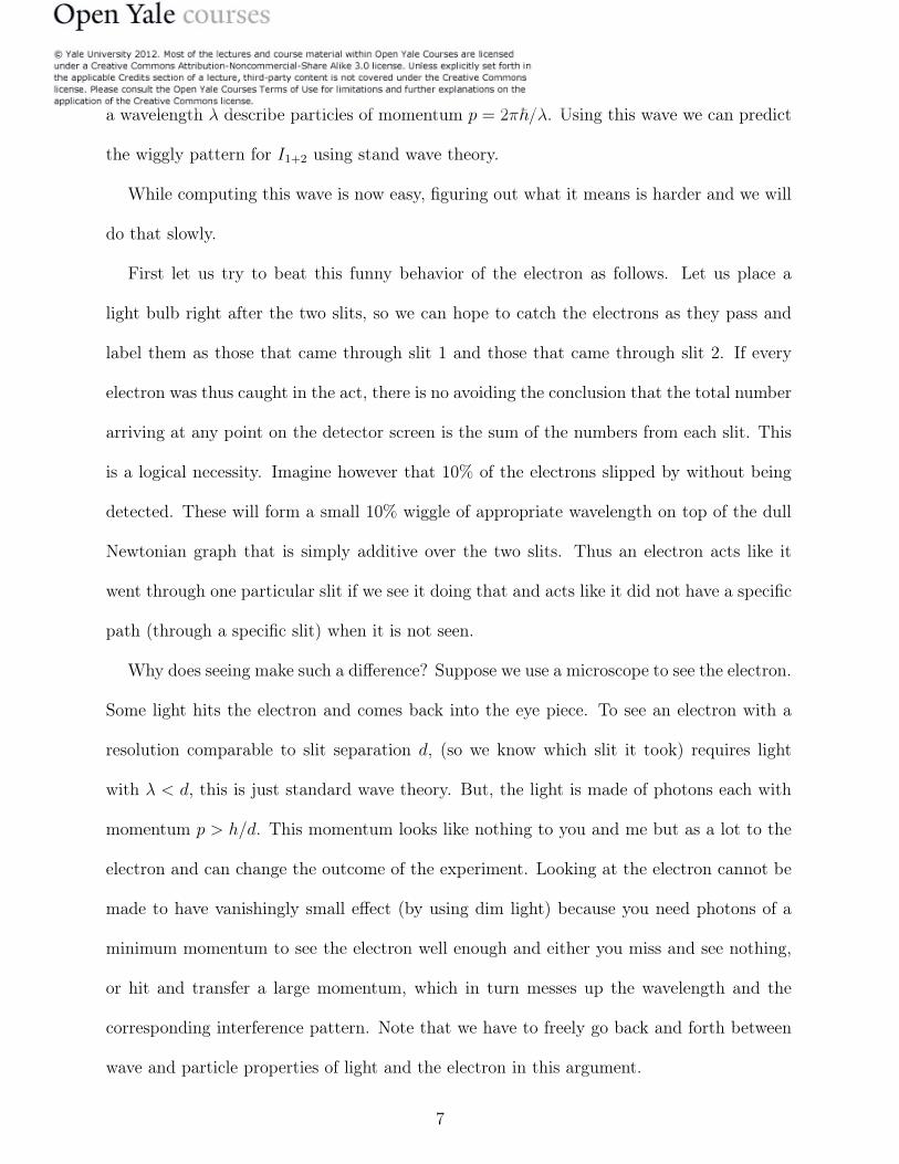
momentum transferred to the electron in the act of observation. Consider Fig.3, which

θ

xd

Figure 3: Light, shown by thick arrow comes from below to the microscope vertically, hits an

electron under the opening of width d and goes into the microscope. The aperture d is roughly

∆x, the uncertainty in the location of the electron. Since light diffracts by an angle θ given by

d sin θ = λ, the deflected photon has an uncertain direction, and can have a horizontal component

of momentum ∆px = po sin θ = poλ/d = po∗2π�pod = 2π�

d . The uncertainty relation then follows.

8

describes an attempt to locate an electron somewhere along the x-axis. Light, shown by thick

arrow hits the electron vertically, and goes back into the microscope through an opening

of size d. If there is an electron under the opening, it will reflect the photon (and thus

be "seen"). The aperture d is roughly ∆x, the uncertainty in the location of the electron.

But the reflected photon has an unknown direction since light diffracts by an angle θ given

by d sin θ = λ. So the reflected photon can have a horizontal component ∆px = po sin θ =

poλ/d = po∗2π�pod = 2π�

d . It follows that ∆x∆px � h. ( I use the symbol � to mean rough

equality, since the technical definition of uncertainty has not been been invoked. )

Thus we know the large initial momentum of the photon that went in but not the large

final momentum of the one that entered the microscope because of its angle is uncertain due

to diffraction. So we do not know how much momentum was transferred to the electron.

Hence the electron’s final momentum is unknown even if it was known before the position

measurement.

Note that we again switch back and forth between photons and waves in this argument.

This is unavoidable.

We return to this subject in the next section on the uncertainty principle.

From now on, to learn quantum mechanics, we will focus on the electron. It will stand

for any particles, say neutrons or pi mesons. Later I may switch to saying "particle".

C. Summary so far.

Here is what we have learnt:

• Electrons are particles in that all the energy, momentum and charge are localized at

one point, the point where the electron hits you or a detector.

9

• Associated with each electron of momentum p is a wave with

λ =2π�p

(7)

• In a DSE, this wave can interfere (even if there is just one electron in the room).

The intensity or amplitude-squared of the wave at any point is proportional to the

likelihood or probability of finding the electron there. If the experiment is repeated

many times with one electron at a time, or with a burst of many electrons at one time,

the graph of probability will become a graph of actual arrivals.

• Even if the electron does not have a definite momentum, there is still some wave

ψ(x, y, z) associated it carrying similar probabilistic information. (This is a postulate.)

D. Heisenberg’s Uncertainty Principle

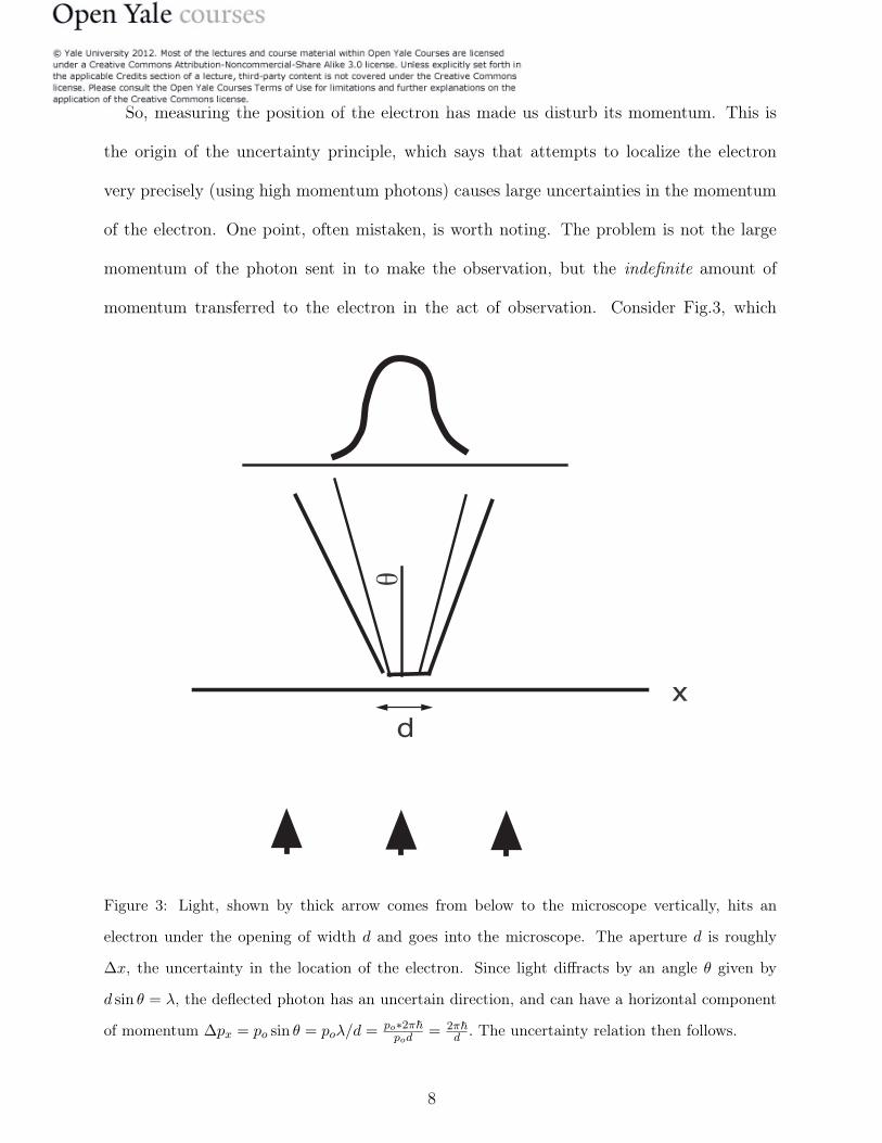
Consider a beam of electrons with momentum p0 in the x-direction, approaching a single

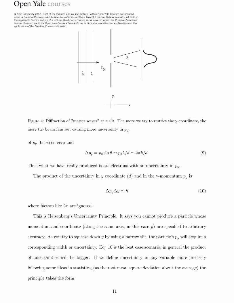
slit of width d in the y-direction as in Fig . 4. Consider an electron just past the slit. It

has a y coordinate known to lie within an interval d, we say we have produced an electron

with position uncertainty ∆y = d. What about its momentum py in the y-direction? It has

no py since the beam was coming along x and we just filtered those with y inside the slit.

By making d smaller and smaller we can produce electrons with arbitrarily well known y

coordinate and momentum.

This is however wrong. This assumption from Newtonian mechanics is false given the

underlying wave. When the wave hits the slit, it will diffract, it will widen to an angle:

d sin θ � λ. (8)

If a screen is placed behind the slit, electrons will reach it in the non-forward direction up to

this angle θ. It means the electrons just past the slit, must have had a corresponding range

10

po

!!

"

x

y

Figure 4: Diffraction of "matter waves" at a slit. The more we try to restrict the y-coordinate, the

more the beam fans out causing more uncertainty in py.

of py- between zero and

∆py = p0 sin θ � p0λ/d � 2π�/d. (9)

Thus what we have really produced is are electrons with an uncertainty in py.

The product of the uncertainty in y coordinate (d) and in the y-momentum py is

∆py∆y � � (10)

where factors like 2π are ignored.

This is Heisenberg’s Uncertainty Principle. It says you cannot produce a particle whose

momentum and coordinate (along the same axis, in this case y) are specified to arbitrary

accuracy. As you try to squeeze down y by using a narrow slit, the particle’s py will acquire a

corresponding width or uncertainty. Eq. 10 is the best case scenario, in general the product

of uncertainties will be bigger. If we define uncertainty in any variable more precisely

following some ideas in statistics, (as the root mean square deviation about the average) the

principle takes the form

11

∆py∆y ≥ �2

(11)

If we are willing to ignore factors of order unity, we may use any reasonable definition of

uncertainty to say

∆py∆y � � (12)

where an approximate inequality is implied.

It follows from the Uncertainty Principle (UP) that a particle of perfectly defined mo-

mentum will have a position about which we know nothing. It has the same odds for being

anywhere !

II. MORE ON ψ

The DSE tells us that electrons do not follow Newtonian trajectories. Instead their fate

is determined by a wave function ψ(x, y, z). All we know so far is that when the particle

has momentum p, the corresponding wave has λ = 2π�p .

So it is reasonable to guess that in the DSE the incoming wave (moving along x) is

ψ(x) = A cos2πx

λ= A cos

px

� (13)

This would certainly produce the desired pattern in the DSE. However it is wrong! It is

wrong because this |ψ(x)|2 oscillates with x, (peaking in some places and vanishing at others)

while a particle of definite momentum is required to have equal preference for all positions

by Heisenberg. But how can a function have a wavelength (as required by the DSE) and its

square not show any variation in x? Here is the escape. Consider the complex function

ψ(x) = Ae2πix

λ = Aeipx� (14)

12

whose real and imaginary parts oscillate with a wavelength λ. Its absolute value squared

|ψ(x)|2 = |A|2 is however a constant since |eiθ| = 1. Note that a complex function is not

invoked in QM as a trick to get to its real part in the end (as in circuits). A complex function

is essential for describing a particle of definite momentum.

Thus we conclude that the probability is not give by the simple square of ψ, namely

ψ2 but the modulus squared |ψ|2 = ψ

∗(x)ψ(x). This makes sense since ψ2 is not positive

definite or even real if ψ is complex.

Now you all know in a double slit experiment how to add two real waves which are out

of step to get an interference pattern. I will show you how two complex waves can do the

same.

The incoming plane wave Aeipx/� will gives rise to two radially outgoing waves of the form

Aeipr/� where r is the radial distance from the slit it comes from, as in Figure 2. Consider

a point on the detecting screen which is r1 from slit 1 and r2 from slit 2. The waves add up

to give

ψ1+2 = Aeipr1/� + Ae

ipr2/� = Aeipr1/�(1 + e

ip(r2−r1)/�) ≡ Aeipr1/�(1 + e

ipδ/�) (15)

The probability is given by

|ψ1+2|2 = |A|2 · |eipr1/�|2 · |eipδ/2�|2|(e−ipδ/2� + eipδ/2�)|2 (16)

where the last factor is just |2 cos pδ2�|

2. Thus

|ψ1+2|2 = 4|A|2 · cos2 pδ

2� (17)

which goes between 4|A|2 at a maximum pδ/� = 2mπ and zero where pδ/� = (2m + 1)π

where m is any integer.

So remember that we must add ψ from the two sources not |ψ|2 so that

I1+2 = |ψ1 + ψ2|2 = (ψ∗1 + ψ∗2)(ψ1 + ψ2) (18)

= |ψ1|2 + |ψ2|2 + ψ∗1ψ2 + ψ

∗2ψ1 (19)

= I1 + I2 + interference terms which are real but indefinite in sign (20)

Similar rules apply if waves from more than two sources are added.

I leave it to you to figure out given de Broglie’s formula relating p to λ that these maxima

( minima) correspond to path differences δ = r2−r1 equal to integral (half-integral) multiples

of λ as with real waves.

13

Thus we will refine the postulates as follows.

• The state of the electron is given by a function, ψ(x), possibly complex.

• The likelihood of finding it at some point x goes as |ψ(x)|2.

• If the electron has a definite momentum p, the wave function is ψ(x) = Aeipx�

A. Relation to classical mechanics

Why does the world look classical (Newtonian) in daily life when we deal with macroscopic

objects, when the underlying physics is quantum mechanical? Why do particles seem to move

on trajectories and why is there no interference on a macroscopic scale? (Think of bullets

coming at you from two holes in the wall instead of one. How can opening a second hole

make your life better?) The question is mathematically the same as the one we have already

explored: "Why does light seem to obey geometrical optics in some situations when it is

actually a wave?" The answer is that if the wave length is much smaller than other lengths

in the problem (like slit widths or separation) we will obtain geometrical optics in the case

of light and Newtonian physics in the case of matter waves.

For example if a particle of mass m = 1Kg moving at 1m/s (so that p = 1 in MKS units)

is shot through a hole of width d = 1m, the diffraction angle will be roughly

sin θ � θ = λ/d = 2π�/p · d � 10−34radians (21)

since except for � � 10−34J · sec, all the other numbers are of order unity in MKS units.

So the particle (or a beam of particles) will emerge from the hole essentially confined in the

transverse direction to the size of the hole. The above beam coming out of the hole will

broaden by 10−10m (the width of an atom) when it hits a screen placed 1024

m ( 1000 times

the size of our galaxy) away. You can replace the meter by a millimeter or the Kg by a

milligram in this example, and the quantum effects (diffraction) will still be absurdly small.

You need to get to atomic dimensions in length and mass to see quantum effects.

If we do a double slit experiment with such a particle using holes 1 m apart, the angle

between successive fringes will be δθ � 10−34rads. If the detecting screen is 1m away, the

spacing between crests will be � 10−34m. This means 10, 000, 000, 000, 000, 000, 000 fringes

will fit into a detector as tiny as the proton (which is 10−15m across) and so we will never

14

see the oscillations. We will see just the average, in which interference terms will get washed

out. We will find I1+2 = I1+I2 which is what we expect in classical mechanics when particles

go via one slit or the other and the number arriving with two slits open is the sum of the

numbers with either one open.

This explains why if bullets are coming at you through a hole in the wall, you cannot

dodge them by opening a a second hole: to profit from the interference zero you will need

to be 10−34m across.

In addition, for the interference pattern to appear, it is essential that the particle not

have any interaction with the outside world: even a single photon that bumps into it can

destroy the interference pattern. While such isolation is readily possible in the atomic scale

it is far from that in the macroscopic scale.

Finally, why do we normally think we can specify the position and momentum of a

particle to arbitrary accuracy when the uncertainty principle says ∆x∆p ≥ � � 10−34J sec?

Consider a particle of mass 1kg. Suppose we know its position to an accuracy of one atom’s

width ∆x � 10−10m. Then ∆p � 10−24 and since m = 1kg, the uncertainty in velocity is

∆v � 10−24m/s. To appreciate how small this is, note that if the particle traveled with

this uncertainty in velocity for 10,000,000 years (� 1014s), the final fuzziness in its position

would be the width of one atom.

B. Role of probability in quantum mechanics

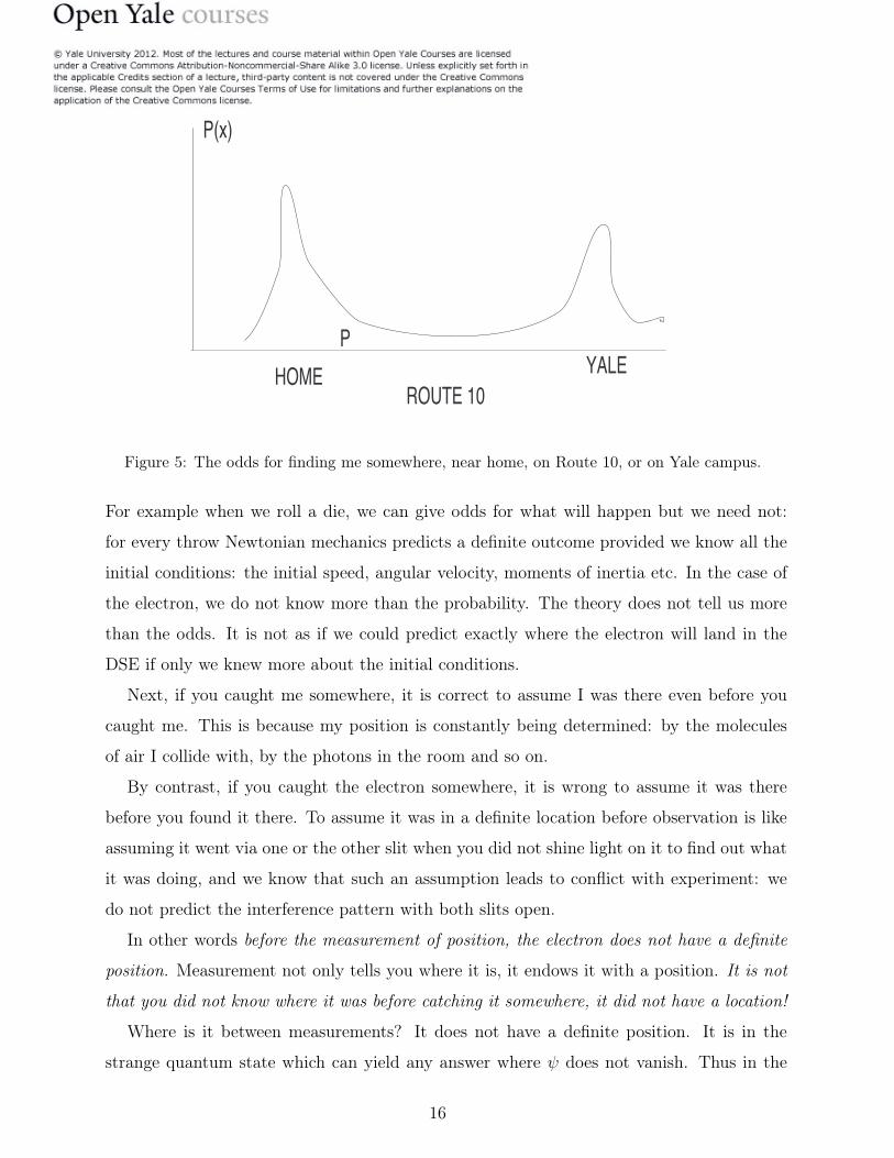
Suppose someone wants to know where I may be found at any given time. By studying

me over some length of time, she can come up a with a plot as in Fig.5. Say you look for

me and find me somewhere, say at the point P . This does not prove her graph is right, you

need to measure my position many times to check this out.

Note that when you do find me, you find all of me in one place: the probability is spread

out but I am not (unless I got into a terrible accident on Route 10). Note also that if you

got me at P , I was actually there at P before you looked.

Suppose the same graph now represents |ψ|2 for an electron and Home and Yale stand for

two nuclei it could be near. If you look for the electron you will find all of it at one place,

its charge is not smeared out in the shape of the graph.

So what is different? First, we use probabilities in classical mechanics as a convenience.

15

HOME YALEROUTE 10

P(x)

P

Figure 5: The odds for finding me somewhere, near home, on Route 10, or on Yale campus.

For example when we roll a die, we can give odds for what will happen but we need not:

for every throw Newtonian mechanics predicts a definite outcome provided we know all the

initial conditions: the initial speed, angular velocity, moments of inertia etc. In the case of

the electron, we do not know more than the probability. The theory does not tell us more

than the odds. It is not as if we could predict exactly where the electron will land in the

DSE if only we knew more about the initial conditions.

Next, if you caught me somewhere, it is correct to assume I was there even before you

caught me. This is because my position is constantly being determined: by the molecules

of air I collide with, by the photons in the room and so on.

By contrast, if you caught the electron somewhere, it is wrong to assume it was there

before you found it there. To assume it was in a definite location before observation is like

assuming it went via one or the other slit when you did not shine light on it to find out what

it was doing, and we know that such an assumption leads to conflict with experiment: we

do not predict the interference pattern with both slits open.

In other words before the measurement of position, the electron does not have a definite

position. Measurement not only tells you where it is, it endows it with a position. It is not

that you did not know where it was before catching it somewhere, it did not have a location!

Where is it between measurements? It does not have a definite position. It is in the

strange quantum state which can yield any answer where ψ does not vanish. Thus in the

16

double slit example, we know when the electron is emitted (since the source recoils) and

when it is detected (when the detector recoils). What happened in between? We may like

to think it followed a definite path via one of the slits. This reasonable assumption is however

false, it will predict I1+2 = I1 + I2.

Instead of considering the position of an electron which can take a continuum of values,

consider a quantum bit or qubit which can be in a state 0 or 1 when measured. But it can

also be in a state when it can yield 0 or a 1. While the classical bit in your PC can also

yield 0 or 1, if it yields 1, we know it was in the state 1 before you looked. On this trial it

could not have yielded any other answer since it was really in the state 1! The qubit on the

other hand is not in any particular state before you measure, the same qubit, on the same

trial, is capable of giving either answer. Only upon measurement does it pick a state. This

is not different from an electron that is not going through any one slit.

Confused? You wont be, when we are done. It will not get less weird, it will just become

more familiar.

C. Normalization

The notion of probability density may be new to you. If you throw a die, you can get six

answers and you can assign probabilities P (1)...P (6) to each outcome. You can make sure

they add up to 1:�

i P (i) = 1. On the other hand, the location of a particle is a continuous

variable and no one point can get a finite probability. Instead a region of width dx gets a

probability P (x)dx. We will demand that our ψ(x) obeys the normalization condition�

all space

P (x)dx =

�

all space

|ψ(x)|2dx = 1. (22)

which just means the particle is somewhere with unit probability.

Suppose I give you the following ψ(x), I will call a "box function" because of its appear-

ance:

ψ(x) = A for|x| < a 0 for |x| > a (23)

where A is a constant, possibly complex. Note that no matter what A is we can say

"The particle clearly has equal chance of being found anywhere within a of the origin

and no chance of being further out."

17

This is a complete description of the relative odds. However it will be more convenient if

ψ is normalized, i.e, obeys Eq 22.

Since �

all space

|ψ(x)|2dx = |A|2 · 2a, (24)

if we choose A = 1√2a

, we get a ψ that is normalized and P (x) = |ψ(x)|2 will give the absolute

probability density. Choosing the overall scale like A in this manner is called "normalizing

the wave function".

While in the case of the string, the string with displacement ψ(x) is physically differ-

ent from the string with displacement 2ψ(x), in QM doubling the wave function describes

the same physical condition, i.e., same relative probabilities. From this family of ψ’s we

traditionally pick one which is normalized.

The following analogy may help. Suppose I tell you that a die has equal chance of giving

any number from 1 to 6 and zero chance of giving anything else. This is a statement of

relative probabilities. Thus the probability for each number from 1-6 could be 3. But these

do not add up to 1, they add up to 18. If I divide all the odds by 18, I get 1/6 for each and

these are absolute probabilities that add up to 1. Usually the word "probability" stands for

absolute probability. It need not. For example we say the odds are 50-50 it will rain. These

add up to 100 but still give the right relative odds. Dividing by 100, we get the absolute

probabilities of 12 for each possibility.

In QM we will try to always work with normalized ψ’s and say so explicitly when we do

not.

III. MOMENTUM WAVE FUNCTIONS

Let us focus on particle living in one dimension. Draw any decent function ψ(x) you

like and it describes a possible state of a quantum particle. Once you rescale it so it is

normalized, you can read off the absolute probability density P (x) = |ψ(x)|2 for any x. We

did this for the rectangle shaped "box" function in Eq. 23.

But look at a particle in a state of momentum p:

ψp(x) = eipx/� (25)

18

where the subscript p tells us it is not any old ψ, it is one that describes a particle of definite

momentum. In QM a particle of definite p has a definite λ as this function does.

Now this ψp(x) is not normalized. So let us multiply it by a number A and choose A so

that we get a normalized function:�

all space

|A|2|eipx� |2dx =

�

all space

|A|2dx = |A|2L = 1 (26)

where L is the length of all space. But this L =∞ and no choice of A will do! This problem

can be dealt with mathematical tricks but we take an easier way out. Let us pretend we

live in a one dimensional universe that is closed but finite, i.e., a circle of circumference

L = 2πR. In this world you can see the back of your head and get hit by a rock thrown

away from you ! But look at the bright side: A normalized state of momentum exists:

ψp(x) =1√L

eipx� (27)

If you are not sure our universe is finite, you can make L as large as you like and assume

reasonably that what happens light years away cannot effect QM on our planet.

This situation also describes real laboratory problems in nanophysics, where an electron

is forced to live on a tiny ring of circumference L.

Remarkably, a particle in such a ring or circle cannot have all possible values of p. This

is because if we start at a point x and follow ψ around the ring we end up with ψ(x + L).

But we are back to the same point and ψ must return to its initial value, ψ(x). That is we

demand

ψ(x) = ψ(x + L) (28)

This is the condition that ψ is single valued or periodic.

When applied to states of definite momentum this requires

eipx/� = e

ip(x+L)/� = eipx/�

eipL/� (29)

which means

eipL/� = 1 (30)

which means the allowed values of p are limited to

p =2π�m

L≡ pm m = 0,±1,±2.. (31)

19

This is the first example of "quantization". In classical mechanics, a particle forced to

live on a circle can have any momentum, in QM, the condition that ψ be single-valued forces

the momentum to be quantized into integral multiples of 2π�L .

If you follow the real or imaginary part of ψ single-valuedness means that the waves must

finish an integral number of oscillation as we go around the ring.

Since L/2π = R, the above condition can be written as the quantization of angular

momentum into integral multiples of �:

pR = m� (32)

Since each allowed value of p is labeled by an integer m, we can label the wave function

by m and write

ψm(x) =1√L

e2πimx

L (33)

In this version the periodicity is evident: adding L to any x, merely adds 2πm to the phase

of the exponential.

IV. SUPERPOSITION AND MEASUREMENT

Before proceeding let us recall the kinematics and dynamics in the Newtonian world. Re-

call that kinematics is what you need to characterize the system fully at one time. Dynamics

is how the description evolves with time.

The complete state of the particle is given by its position x and momentum p = mv. If you

know this, you the value of all other "dynamical variables" which means things like kinetic

energy K = 12mv

2 = p2

2m , angular momentum L = r × p and total energy E = p2

2m + V (x)

where V (x) is the potential energy. Note that the formula for E varies from problem to

problem depending on what forces act on a particle (spring, gravity etc.) while expressions

for K, L are fixed. The range for x and p is any real number. However a particle forced to

live on a ring may have its position limited to points on the ring. Its momentum however

always can assume any real value.

The dynamics is given by F = ma or F = dpdt . Since F (x(t)) = −dV/dx, the force at

time t is determined by where the particle is. If at some time t, we start at some point with

some momentum, the position a little later is controlled by p(t) (which is essentially v(t)

20

the velocity) and the momentum a little later is controlled by F (x(t)). This way we inch

forward in time.

Let us examine the corresponding rules in QM. They have the form of postulates. We

will discuss a few now and finish it in later lectures.

Postulate: In QM, the complete information about the particle is given by a

(possibly complex) wave function ψ(x).

Given this ψ you can ask where is the particle? That is, if I measure its position, what

answer will I get? The answer is you can find it any place where ψ is nonzero and the

probability density is P (x) = |ψ(x)|2.

Next you can ask what you will get if you measure its momentum. The information is

contained in ψ(x) itself. However it takes more work than simply finding |ψ|2, which was

the case for P (x).

The following postulate tells us how.

Postulate: The probability of obtaining a value p is

P (p) = |Ap|2 (34)

where Ap is defined as the coefficients in the expansion of the normalized ψ(x) as a sum

over normalized wave functions ψp(x) of definite momentum

ψ(x) =�

p

Ape

ipx�√

L≡

�

p

Apψp(x) =�

m

Amψm(x). (35)

You may ask two questions at this point.

1. How do we know every given ψ can be written as a sum over wavefunctions of definite

momentum?

2. How are we to find Ap or Am?

The first question is answered by appealing to a theorem in mathematics without giving

the proof. If you want to know more look up Fourier Series.

The answer to the second is that

Ap =

� L

0

1√L

e− ipx

� ψ(x)dx ≡� L

0

ψ∗p(x)ψ(x)dx. (36)

Or in terms of m

21

Am =

� L

0

1√L

e− 2πimx

L ψ(x)dx ≡� L

0

ψ∗m(x)ψ(x)dx. (37)

Note that Am and Ap stand for the same thing: their mod-squares give the probability

for having momentum p = 2πm�/L. I will use them interchangeably.

For those who want to know more about determining Am, here are some details.

Consider a vector V in three dimensions. We know it can be written as follows

V = iVx + jVy + kVz ≡3�

i=1

Viei (38)

where the basis vectors e1 = i, e2 = j, e3 = k obey orthonormality condition

ei · ej = 1 if i = j (39)

= 0 if i �= j (40)

≡ δij (41)

The Kronecker delta, δij, is defined to be 1 if the indices i and j are equal, zero otherwise.

Thus for example δ11 = 1, δ13 = 0.

The term orthonormal means the basis vectors are mutually perpendicular (orthogonal)

and normalized ( are of length 1).

Suppose you have in mind some arbitrary vector V pointing in some direction and of

some length and you want to write it in terms of the basis vectors as in Eq. 38. How do

we choose the components Vi? By using the orthonormality conditions in Eq. 41 as follows.

Say you want V2. Take the dot product of both sides of Eq. 38 with e2:

V · e2 =

�3�

i=1

Viei

�· e2 =

3�

i=1

Vi (ei · e2)� �� �δi2

= V2. (42)

We have used the fact that since ei · e2 = δi2 it vanishes if i �= 2 and gives 1 if i = 2, thereby

pulling out just V2 from the sum.

Consider now the functions

ψm(x) =1√L

e2πimx/L

m = 0,±1,±2.. (43)

These obey � L

0

ψ∗m(x)ψn(x)dx = δmn (44)

22

a fact you may easily verify: if m = n, the exponentials cancel and the integral of 1/L gives

1, while if m �= n, the real and imaginary parts of the exponential oscillate over |m− n| full

cycles and give zero.

Thus ψm(x) are orthonormal basis functions (like ei are basis vectors), and the dot

product ei · ej is replaced by�

ψ∗i (x)ψj(x).

Consider the sum

ψ(x) =�

m

Am1√L

e2πimx/L =

�

m

Amψm(x) (45)

If we multiply both sides of Eq. 45 by ψ∗n(x) and integrate, we will find Eq.37

� L

0

1√L

e−2πinx

L ψ(x)dx = An (46)

because (as in the case three dimensional vectors)�

ψ∗n(x)ψ(x)dx =

�ψ∗n(x)

�

m

Amψm(x)dx (47)

=�

m

Am

�ψ∗n(x)ψm(x)dx

� �� �δmn

= An (48)

Here is a summary of the correspondences:

V =3�

i=1

Viei ⇔ ψ(x) =�

m

Ame

2πmx�√

L≡

�

m

Amψm(x) (49)

ei · ej = δij ⇔� L

0

ψ∗m(x)ψn(x)dx = δmn (50)

Vi = V · ei ⇔ Am =

� L

0

1√L

e− 2πimx

L ψ(x)dx ≡� L

0

ψ∗

mψ(x)dx (51)

In three dimension we know that linear combinations of the three basis vectors ei can

reproduce any vector we want. If you want, that is what defines three dimensions. In the

case of functions, we have an infinite number of basis functions ψm(x) and we also need to be

able to reproduce an arbitrary periodic function ψ(x). To show that our set is "complete"

i.e., capable of handling any function ψ(x), is too hard to prove and you were asked to take

it on faith.

Let us now consider some examples of how the postulate is used.

Consider

ψ(x) = N cos6πx

L(52)

23

where N is some constant. First note that this is an allowed function since it is periodic

under x → x + L. Next we can choose N to normalize this ψ. Since the average value of

cos2 over any number of full cycle is 1/2, the choice N =�

2/L does the job:

ψ(x) =

�2

Lcos

6πx

L(53)

Next we write it in terms of complex exponentials

ψ(x) =

�2

L

1

2

�e

6πixL + e

−6πixL

�=

�1

2

�e

6πixL

√L

+e−6πix

L

√L

�(54)

Comparing to the normalized basis function

ψp =e

ipx/�√

L

we see that the first term corresponds to p = 6π�L and the second to p = −6π�

L , or what we

would call m = ±3 and that

A±3 =1√2

.

How about the odds for m = ±3? We see that

P (m = 3) = P (m = −3) =1

2. (55)

It will be a good exercise for you to repeat this analysis with

ψ = 5 cos2(2πx/L) + 2 sin(4πx/L)

This is one problem, it is better not to normalize ψ and to find the handful of nonzero Ap’s

that give relative probabilities. Dividing by the sum of these nonzero probabilities then gives

the absolute probabilities.

In this problem we did not do any integrals to find Am, i.e., we did not invoke Eq. 37

because the given function was already in the form of a sum over functions of the form

ψm(x) � e2πimx/L.

Now I will give an example of a function where we need to do some work to find Am.

Let

ψ(x) = Ne−α|x| −L

2 ≤ x ≤ L2 , αL >> 1 (56)

24

x=0

x=-L/2,x=L/2

ψ

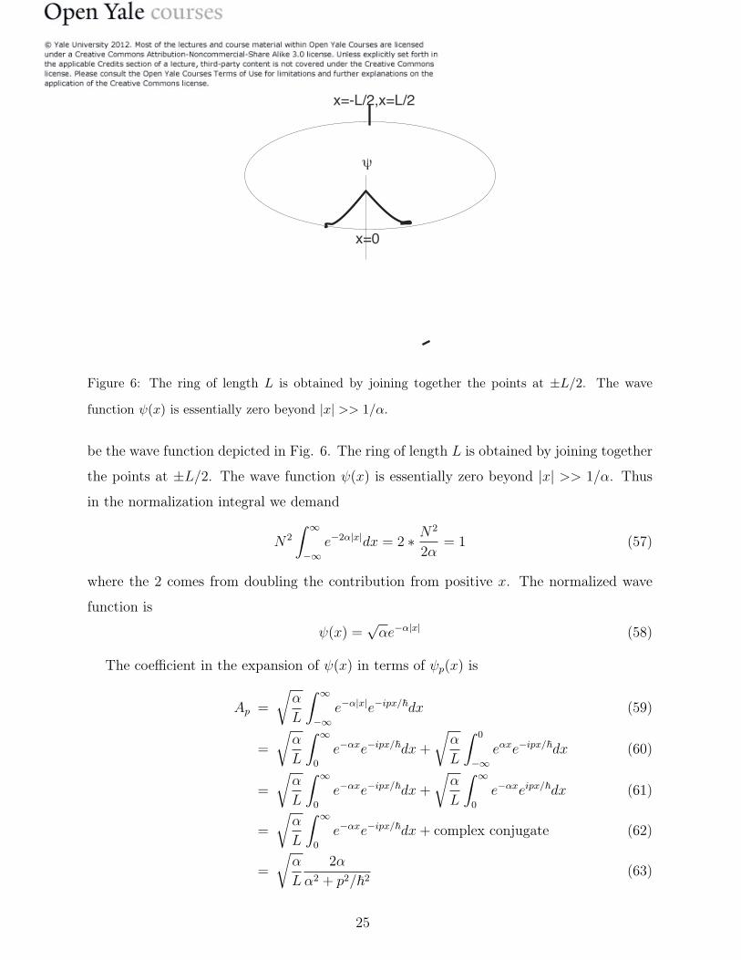
Figure 6: The ring of length L is obtained by joining together the points at ±L/2. The wave

function ψ(x) is essentially zero beyond |x| >> 1/α.

be the wave function depicted in Fig. 6. The ring of length L is obtained by joining together

the points at ±L/2. The wave function ψ(x) is essentially zero beyond |x| >> 1/α. Thus

in the normalization integral we demand

N2

� ∞

−∞e−2α|x|

dx = 2 ∗ N2

2α= 1 (57)

where the 2 comes from doubling the contribution from positive x. The normalized wave

function is

ψ(x) =√

αe−α|x| (58)

The coefficient in the expansion of ψ(x) in terms of ψp(x) is

Ap =

�α

L

� ∞

−∞e−α|x|

e−ipx/�

dx (59)

=

�α

L

� ∞

0

e−αx

e−ipx/�

dx +

�α

L

� 0

−∞e

αxe−ipx/�

dx (60)

=

�α

L

� ∞

0

e−αx

e−ipx/�

dx +

�α

L

� ∞

0

e−αx

eipx/�

dx (61)

=

�α

L

� ∞

0

e−αx

e−ipx/�

dx + complex conjugate (62)

=

�α

L

2α

α2 + p2/�2(63)

25

P (p) = |Ap|2 =4α3

L

�1

α2 + p2/�2

�2

(64)

Note that P (p) is peaked at p = 0 and falls rapidly. When p/� = α the function drops

to 1/4 of it speak value If we take this to be the uncertainty in p (just for an order of

magnitude) we can say

∆p = �α =�

∆x(65)

which is in accord with the uncertainty principle: as we squeeze the function in x it broadens

out in p in such a way that ∆p∆x � �.

A. Collapse of ψ.

Postulate: Collapse of the wave function: If a measurement of position gives

a value say x = 3, the wave function (originally spread out in x) will collapse to

a spike at x=3, if a measurement of momentum gives rise to a value say m = 3,

the wave function (originally a sum or superposition over momentum states as

in Eq. 35) will collapse to that particular state.

Consider an example. We begin with the state ψ(x) =√

αe−α|x|. It is peaked near the

origin and has a width ∆x � 1/α. We saw that

ψ(x) =�

p

Apψp(x) where Ap =�

αL

2αα2+p2/�2 (66)

This means every p = 2π�m/L is a possible result in a momentum measurement, since

|Ap|2 does not vanish for any (finite) p. Suppose the measurement yields p = 6π�m/L

which corresponds to m = 3. Right after the measurement, the state of the particle, which

used to a sum over all p, now collapses to just ψ3(x) = e6πi�/L

/√

L. If you immediately

remeasure momentum you will get m = 3. But if you measure position, it can be anything

on the ring, each x having the same probability since |ψ3(x)|2 = 1/L is x-independent.

Thus we went from a state that had a reasonably sharp position δx � 1/α (assuming α is

large) and a large spread in possible momentum (∆ � �α) to one where the momentum

was sharply defined (m = 3) but the position was totally unknown. If we make another

position measurement and find it near x = 6, ψ will collapse to a spike near x = 6 and

its (range of possible ) momentum will again be very spread out. Thus you cannot make

a state with sharply defined x and p. However if the particle is macroscopic (1kg) and it

26

has say ∆x � 10−17m and ∆ � 10−17

kgm/s, that particle has a well defined position and

momentum for all practical purposes.

V. STATES OF DEFINITE ENERGY

Now we ask for wave functions ψE(x) that describe a particle in a state of definite energy

E. Such states are important because if we shine light on a system it will absorb energy and

go from a state of initial energy Einitial to a state of final energy Efinal only if the incident

radiation has a frequency f such that the photon energy satisfies hf = Efinal − Einitial.

Likewise it will emit a photon of frequency f where �ω = hf = Einitial −Efinal. So we need

to know what the allowed energies are.

In classical mechanics, if you know x and p (by measuring them) you need not measure

energy, it is given by

E =p

2

2m+ V (x). (67)

In the quantum case a measurement of x may give a precise answer but ψ collapses to a

state of totally indeterminate p and vice versa. So we cannot deduce the value of E from

these measurements (with one exception: when V (x) ≡ 0 , E is simply p2/2m.)

What we need to do is to measure E as a independent entity, with its own set of functions

ψE(x) that describe a particle in a state with definite energy E and give the odds P (E) =

|AE|2.

So here is the recipe.

Step 1: Find ψE(x) by solving the equation (called the time-independent Schrödinger

Equation)

− �2

2m

d2ψE(x)

dx2+ V (x)ψE(x) = EψE(x) (68)

Step 2: Write the given ψ(x) (after normalizing it) in terms of normalized functions ψE(x)

which describe particles in a state of definite energy:

ψ(x) =�

E

AEψE(x) (69)

Step 3: Then

P (E) = |AE|2 AE =

�ψ∗E(x)ψ(x)dx. (70)

Note the following:

27

• The functions ψE obey an equation that depends on the potential V (x) the particle

experiences. This for each context we will need to find the new set of ψE(x)�s. For

example if V (x) = 12kx

2 there will be one set of functions and the corresponding set

of allowed energies, while if V (x) = Ax4 a new set has to be determined.

• Solutions will typically exist only for some values of energy E, just as solutions existed

only for some values of p on a circle. Thus energy will be quantized.

To summarize once and for all if a normalized ψ(x) is expanded in terms of nor-

malized ψp or normalized ψE, |Ap|2 or |AE|2 give the absolute probabilities for

obtaining momentum p or energy E.

In some problems where we can tell by inspection that only a handful of nonzero A�s

exist, we may be better off dividing the relative probabilities |A|2 by�

E |AE|2 or�

p |Ap|2

to get the absolute probabilities, than doing the x-integral of |ψ(x)|2 to normalize ψ(x).

A. Solving for ψE

Let us take the simplest of cases a free particle with V (x) = 0. The equation is

− �2

2m

d2ψE(x)

dx2= EψE(x) (71)

which can be rewritten as

ψ”E(x) +

2mE

�2ψE = 0 (72)

where ψ” stands for the second derivative of ψ. Let us rewrite this further as

ψ”E(x) + k

2ψE = 0 (73)

where

k2 =

2mE

�2E =

�2k

2

2m. (74)

The general solution to this is

ψ(x) = Aeikx + Be

−ikx (75)

These is clearly a superposition of states of momentum p = �k and p = −�k where p is

related to E by

E =�2

k2

2m=

p2

2m(76)

28

Even in classical mechanics a free particle of energy E will have momentum p = ±√

2mE

obeying p2

2m = E. However it will have to pick one sign or another sign of momentum at any

given instant. What is new here is that in QM it can be in a state that can give either sign.

If the particle is in a ring, there is another nonclassical feature: momentum will be

quantized to

pn =2π�L

n n = 0,±1,±2... (77)

and E will be quantized to

En =p

2n

2m=

4π2�2n

2

2mL2(78)

The reason for quantizing p is as before: to make sure ψ is single valued and returns to itself

under x→ x + L.

Note an interesting fact. In this problem states of definite momentum p are also states

of definite energy E = p2/2m. However states with p and −p have the same energy. So

a state of definite energy is not in general a state of definite momentum since it can be a

superposition of states with opposite values of p as in Eq. 75. However we can pick states

with just A �= 0, B = 0 or vice versa to get states with well defined energy and momentum.

We say there are two states at each energy and that we have a degeneracy, i.e., a term that

signifies that there is more than one state at a given energy.

Note that this system can absorb light only at certain frequencies, namely those obeying

hf = �ω = Ef − Ei (79)

where the indices f and i are the final and initial values of the integer n in Eq. 78 with

f > i. A similar result holds for emission as it drops in energy.

VI. THE RECIPE: AN OPTIONAL SECTION

When asked about states of definite energy, you were asked to first solve differential

equation, whereas when I described momentum states, I just said they are given by

ψp(x) =1√L

eipx/� (80)

Instead I could have said ψp are the functions that solve the equation

−i�∂ψp(x)

∂x= pψp(x) (81)

29

Likewise I said that a state of definite position is a spike in the infinitesimal neighborhood

of x0 and zero or negligible elsewhere.

I could just as easily have specified states of well defined position as solutions to an

equation. Let ψx0(x) describe a particle localized at x0. It is the solution to

xψx0(x) = x0ψx0(x). (82)

Equations 81 and 82 are called eigenvalue equations for x and p. The name means the

following. Suppose you take a function f(x) and do something to it like taking its derivative.

This will give a new function: for example sin x will go into cos x. Let us denote this as

follows:

D sin x = cos x. (83)

Likewise Dx3 = 3x2 and DLnx = 1/x. Is there a function which is unaffected by this

operation, except for being multiplied by some number? In other words, is there an f(x)

that obeys

Df = af(x) (84)

where a is a constant? The answer is affirmative, and the solution is Aeax because

Df = D(Aeax) = aAe

ax = af. (85)

When this happens we say Aeax is an eigenfunction of the operation D and a is the eigenvalue.

Is there an eigenfunction for −iD, i.e., can we find a function such that

−idf

dx= pf(x)? (86)

The answer is of course f(x) = Aeipx/� since

−id(Ae

−ipx/�)

dx= pAe

−ipx/� (87)

Thus ψp(x), the states of definite momentum p are eigenfunctions of −i�D and p is the

corresponding eigenvalue.

One can imagine doing more such things to a function using derivatives: you can consider

D2f , which means taking the second derivative.

But consider another line of operations which is to multiply a function f(x) by x. This

too in general changes the function: if you take sin x and multiply it by x, it becomes a

different function, x sin x. Can we ever find a function such that

xf(x) = cf(x) (88)

30

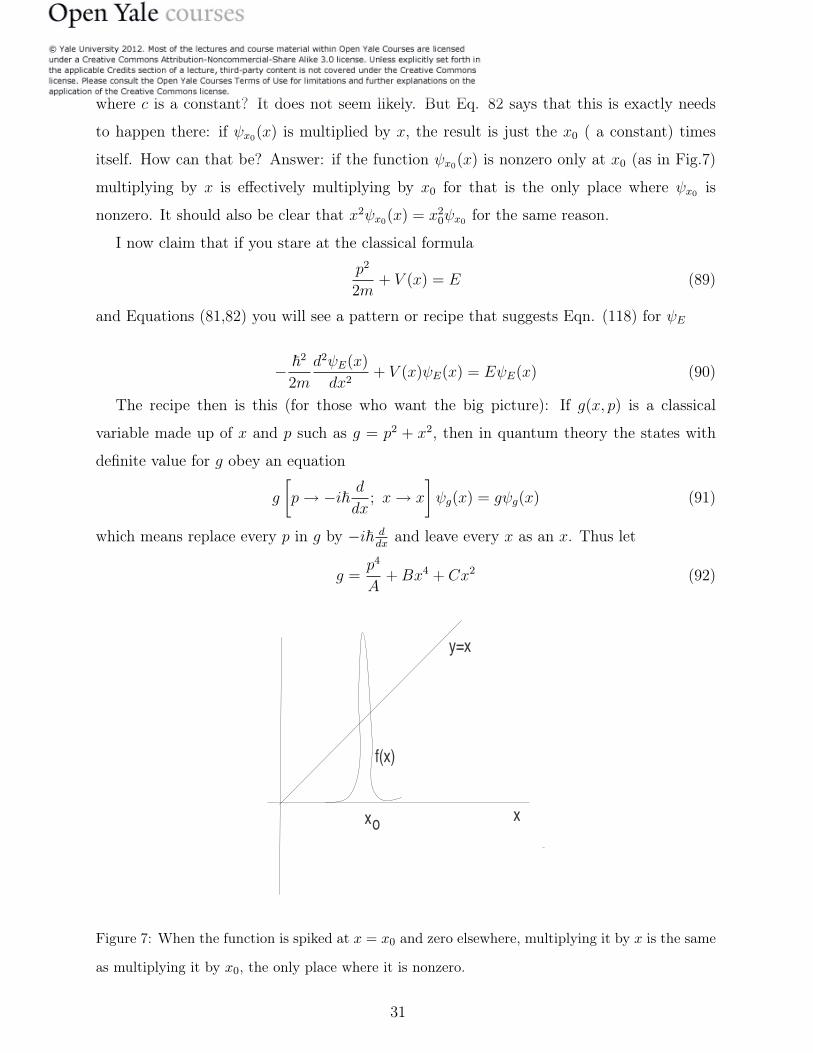
where c is a constant? It does not seem likely. But Eq. 82 says that this is exactly needs

to happen there: if ψx0(x) is multiplied by x, the result is just the x0 ( a constant) times

itself. How can that be? Answer: if the function ψx0(x) is nonzero only at x0 (as in Fig.7)

multiplying by x is effectively multiplying by x0 for that is the only place where ψx0 is

nonzero. It should also be clear that x2ψx0(x) = x

20ψx0 for the same reason.

I now claim that if you stare at the classical formulap

2

2m+ V (x) = E (89)

and Equations (81,82) you will see a pattern or recipe that suggests Eqn. (118) for ψE

− �2

2m

d2ψE(x)

dx2+ V (x)ψE(x) = EψE(x) (90)

The recipe then is this (for those who want the big picture): If g(x, p) is a classical

variable made up of x and p such as g = p2 + x

2, then in quantum theory the states with

definite value for g obey an equation

g

�p→ −i� d

dx; x→ x

�ψg(x) = gψg(x) (91)

which means replace every p in g by −i� ddx and leave every x as an x. Thus let

g =p

4

A+ Bx

4 + Cx2 (92)

f(x)

x

y=x

xo

Figure 7: When the function is spiked at x = x0 and zero elsewhere, multiplying it by x is the same

as multiplying it by x0, the only place where it is nonzero.

31

be a variable in classical mechanics. (It has no name like kinetic energy or angular momen-

tum but it does not appear anywhere except in this example). Then functions that describe

states of definite g are

�2

A

d4ψg(x)

dx4+ Bx

4ψg(x) + Cx

2ψg(x) = gψg(x) (93)

If you want to test yourself, ask what equation is obeyed by ψl(x, y, z) which describes a

particles of definite angular momentum l around the z-axis. Remember in classical physics

L = r× p (94)

so that in the z-direction

Lz = xpy − ypx. (95)

Ready? The answer is

x

�−i�∂ψl

∂y

�− y

�−i�∂ψl

∂x

�= lψl(x, y, z) (96)

VII. THINKING INSIDE THE BOX

Consider a particle in a potential

V (x) = 0 0 < x < L "the box" V (x) =∞ outside the box (97)

depicted in Fig. 8.

First consider ψ outside the box, keeping V0 finite but arbitrarily large for now. Clearly

any finite energy I pick will obey E < V0 outside the box. This means

k� =

�2m(E − V0)

�2= iκ κ =

�2m(V0 − E)

�2(98)

and the solution will assume the form (upon using e±ik�x = e

∓κx),

ψ(x) = Aeκx + Be

−κx (99)

In the region to the right of the box, we reject the first term because it diverges exponentially

as x → ∞ and cannot be normalized. Similarly we drop the exponentially rising term to

the left of the box.

32

Note that the region outside the box is disallowed clasically, since with E < V0 the

kinetic energy has to be negative. It is the negative kinetic energy that has made k� into the

imaginary κ and changed the oscillatory exponential to a decaying exponential. Amazingly

the particle has a nonzero probability to be in this region. This region has a width of order

1/κ.

As V0 grows, the exponential fall becomes more and more rapid, and in the limit V0 →∞,

we see κ→∞ as well and ψ vanishes as soon as we leave the box. Thus when V0 is infinite,

the particle cannot leave the box even in quantum theory.

Inside the box where V = 0 we solve

ψ” + k

2ψ = 0 k =

�2mE

�2(100)

We could write down the solution in terms of exponentials but with my infinite wisdom I

will use trigonometric functions. You can satisfy yourselves that

ψ(x) = A cos kx + B sin kx (101)

satisfies the equation for any A and B. If any k is allowed so is any energy since

E =�2

k2

2m. (102)

n=1

n=2

x=0 x=L

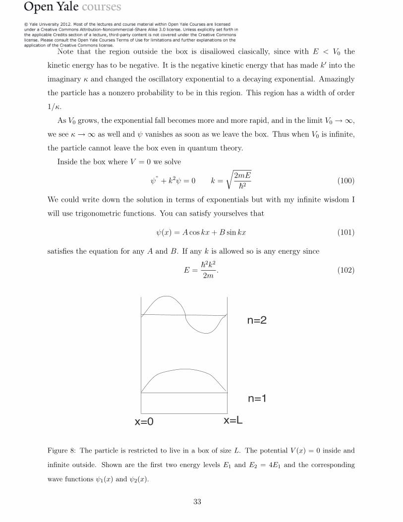
Figure 8: The particle is restricted to live in a box of size L. The potential V (x) = 0 inside and

infinite outside. Shown are the first two energy levels E1 and E2 = 4E1 and the corresponding

wave functions ψ1(x) and ψ2(x).

33

However ψ has to vanish at both ends since it vanishes identically outside the box. The

condition ψ(0) = 0 tells me A = 0 while the condition ψ(L) = 0 tells me

B sin kL = 0. (103)

Since I do not want B = 0, which completely kills the solution, I demand

kL = nπ, n = 0, 1, 2, 3, (104)

Note that n = 0 is not allowed since then ψ ≡ 0. As for negative n, it gives −1 times the

solution at positive n since sin(−x) = − sin x.) But ψ and −ψ (indeed any multiple of ψ )

describe the same state.

Thus the allowed energies are labeled by n

En =�2

n2π

2

2mL2n = 0, 1, 2, 3, (105)

and the normalized wave functions also labelled by n are

ψn(x) =

�2

Lsin

�nπx

L

�. (106)

Note that the lowest energy in a box would have been zero classically: you just sit still

on the floor. Quantum mechanically such a state is disallowed by the uncertainty principle.

Here is how you can make a quick estimate of the lowest energy. (In this argument factors

of 2, π etc., will be ignored. It goes as follows. Since ∆x � L, ∆p ≥ �/L and

E =p

2

2m≥ �2

mL2

which agrees (up to these factors) with E1.

This artificial example gives you all the key ideas. You can consider a whole set of po-

tentials, say 12kx

2 corresponding to an oscillator. The following features will always emerge.

If the potential is such that the particle can classically escape to infinity at the given

energy (E > V (±∞)), ψ will be oscillatory everywhere. In regions where the classical

kinetic energy would have been large, it will oscillate more rapidly. Energy will not be

quantized, i.e., at any real energy you will have solutions.

If E < V (±∞) so that the particle is not allowed at spatial infinity, ψ will die exponen-

tially as soon as you cross the classical turning points. It will be found that such a solution

34

(vanishing at both ends of space) can occur only at some special values of energy. In other

words bound states will have discrete quantized energies.

Finally the lowest energy will never be zero as in classical mechanics: particle sitting still

at the minimum of V (x) (assumed to be V = 0). The minimum energy can be estimated

using the uncertainty principle with a little more effort.

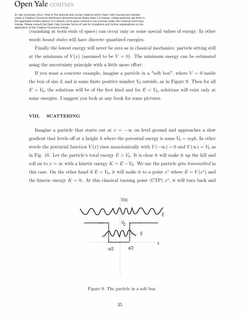
If you want a concrete example, imagine a particle in a "soft box", where V = 0 inside

the box of size L and is some finite positive number V0 outside, as in Figure 9. Then for all

E > V0, the solutions will be of the first kind and for E < V0, solutions will exist only at

some energies. I suggest you look at any book for some pictures.

VIII. SCATTERING

Imagine a particle that starts out at x = −∞ on level ground and approaches a slow

gradient that levels off at a height h where the potential energy is some V0 = mgh. In other

words the potential function V (x) rises monotonically with V (−∞) = 0 and V (∞) = V0 as

in Fig. 10. Let the particle’s total energy E > V0. It is clear it will make it up the hill and

roll on to x =∞ with a kinetic energy K = E − V0. We say the particle gets transmitted in

this case. On the other hand if E < V0, it will make it to a point x∗ where E = V (x∗) and

the kinetic energy K = 0. At this classical turning point (CTP) x∗, it will turn back and

a/2-a/2

V

V(x)

0

E

E

x

Figure 9: The particle in a soft box

35

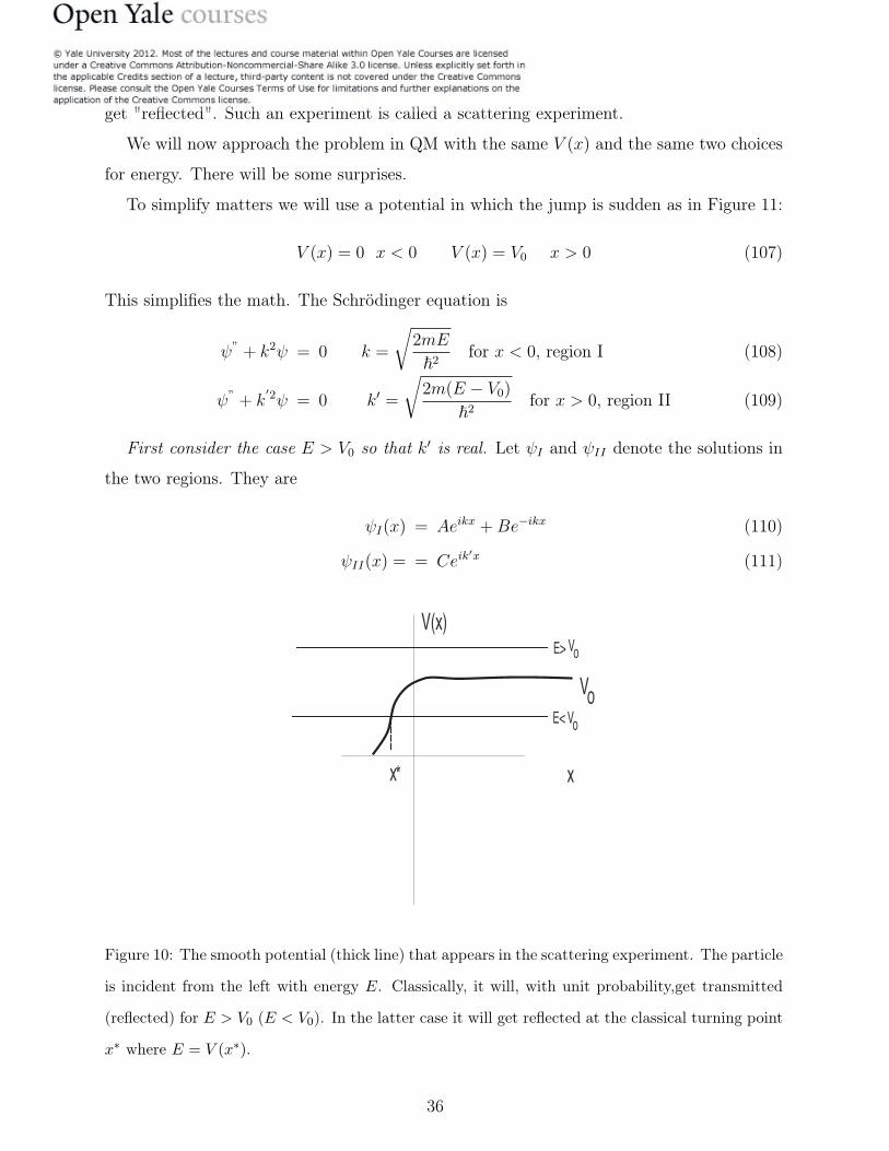
get "reflected". Such an experiment is called a scattering experiment.

We will now approach the problem in QM with the same V (x) and the same two choices

for energy. There will be some surprises.

To simplify matters we will use a potential in which the jump is sudden as in Figure 11:

V (x) = 0 x < 0 V (x) = V0 x > 0 (107)

This simplifies the math. The Schrödinger equation is

ψ” + k

2ψ = 0 k =

�2mE

�2for x < 0, region I (108)

ψ” + k

�2ψ = 0 k

� =

�2m(E − V0)

�2for x > 0, region II (109)

First consider the case E > V0 so that k� is real. Let ψI and ψII denote the solutions in

the two regions. They are

ψI(x) = Aeikx + Be

−ikx (110)

ψII(x) = = Ceik�x (111)

E< Vo

x

V(x)

Vo

E> Vo

x*

Figure 10: The smooth potential (thick line) that appears in the scattering experiment. The particle

is incident from the left with energy E. Classically, it will, with unit probability,get transmitted

(reflected) for E > V0 (E < V0). In the latter case it will get reflected at the classical turning point

x∗ where E = V (x∗).

36

V(x)

x

V0

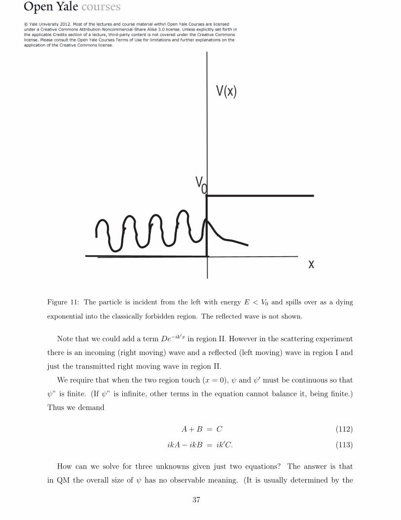
Figure 11: The particle is incident from the left with energy E < V0 and spills over as a dying

exponential into the classically forbidden region. The reflected wave is not shown.

Note that we could add a term De−ik�x in region II. However in the scattering experiment

there is an incoming (right moving) wave and a reflected (left moving) wave in region I and

just the transmitted right moving wave in region II.

We require that when the two region touch (x = 0), ψ and ψ� must be continuous so that

ψ” is finite. (If ψ” is infinite, other terms in the equation cannot balance it, being finite.)

Thus we demand

A + B = C (112)

ikA− ikB = ik�C. (113)

How can we solve for three unknowns given just two equations? The answer is that

in QM the overall size of ψ has no observable meaning. (It is usually determined by the

37

normalization condition, an option that is excluded in infinite space.) So we might as well

choose A = 1. Then we find

B =k − k

�

k + k�(114)

C =2k

k + k�. (115)

The point to note is that the reflected wave has nonzero amplitude B. Thus

a particle with enough energy to go over the hill still has a nonzero probability

to get reflected. It has has less than 100% chance of getting transmitted.

Now consider E < V0. This means

k� =

�2m(E − V0)

�2= iκ κ =

�2m(V0 − E)

�2(116)

(I leave it as an exercise for you to solve for the amplitudes B and C in this case.)

Anyway, in Region II we have

ψII = Ce−κx

. (117)

In other words, there is a nonzero probability of finding the particle to the right of the

classical turning point, x = 0. The odds of finding it deep in the forbidden region however

drop exponentially. Roughly speaking if you go a distance such that κx >> 1, the exponen-

tial becomes negligible. Bigger the value of V0 − E, smaller the spill over to the classically

forbidden region.

Imagine now that the potential drops to zero once again beyond x = a . If κa is not

large, the exponential function would have a decent size at x = a and join smoothly with an

oscillating (k� real) right moving solution for x > a. Thus the particle would have "tunneled"

through a barrier that would have been impenetrable for a classical particle. Note that we

do not really need V to drop to zero, it just has to drop below E for the particle to escape to

infinity. In other words, if two regions where the particle is allowed classically are separated

by a region where it is forbidden, it will leak or "tunnel" from one side to the other. The

leakage rate will decrease rapidly (exponentially) with width and the height of the barrier.

For future use note that if the barrier height is infinite, then so is κ. In this case e−κx = 0

for any x > 0, there is no spill over, and ψ simply vanishes in the forbidden region.

38

IX. TIME DEPENDENT SCHRÖDINGER EQUATION

So far we have focused on one instant in time and learnt how the particle is described

by a ψ(x) and how to extract information from it regarding position, momentum, energy

etc. This is what we call kinematics. Now for the dynamics, i.e., how ψ changes with time.

So first we have to start referring to it as ψ(x, t). This is like saying classically that for

kinematics at any time you need an x and a p to describe it fully and that dynamically x(t)

and p(t) vary with time and describe the particle’s evolution in time. There we had F = ma

and here we have the time-dependent Schrödinger equation (SE):

i�∂ψ(x, t)

∂t= − �2

2m

∂2ψ(x, t)

∂x2+ V (x)ψ(x, t) (118)

At a mathematical level, this is a partial differential equation for a function of two vari-

ables (x, t). Since it specifies the first time- derivative of ψ, it follows that given the initial

ψ(x, 0), its future value ψ(x, t) is determined as above.

Let us not try to solve it for every possible initial ψ(x, 0). As a modest goal let us try to

find a very limited class of solutions of the form

ψ(x, t) = F (t)ψ(x) (119)

This is not generic, generically x and t will all be mixed up together. Let us plug this

into Eq. 118 and see if it admit such a solution.

Bear in mind that the function in question is a product of two functions, one that depends

on just t and one that depends on just x. In the LHS of Eq. 118 we have a partial time

derivative which will act only on the F (t) (while ψ(x) just stands there). On the right hand

side we have only partial derivatives with respect to x. These will act on just ψ(x) (while

F (t) is idling) and on this function they act as total derivatives.

Thus we end up with

ψ(x)i�dF (t)

dt= F (t)

�− �2

2m

d2ψ(x, t)

dx2+ V (x)ψ(x)

�≡ Hψ(x) (120)

where we have defined Hψ to be that combination that occurs frequently. Dividing both

sides by F (t)ψ(x) we find1

F (t)i�dF (t)

dt=

1

ψ(x)Hψ(x) (121)

39

We now see a function of just t being equal to a function of x for all t and x. This means both

functions have to be constants since the function of t alone cannot have any x-dependence

and the function of x alone cannot have any t-dependence. Calling this constant E, we find

1

F (t)i�dF (t)

dt=

1

ψ(x)Hψ(x) = E (122)

which means two equations:

i�dF (t)

dt= EF (t) (123)

�− �2

2m

d2ψ(x, t)

dx2+ V (x)ψ(x)

�= Eψ(x) (124)

Clearly the solution to the first equation is

F (t) = F (0)e−iEt/� (125)

The second equation we recognize to be one that is obeyed by functions of definite energy

E: ψ(x) = ψE(x). Thus we find that the factorized solutions of the form ψ(x, t) = F (t)ψ(x)

do exist and are given by

ψE(x, t) = e−iEt/�

ψE(x). (126)

The factorized solution is telling us that of the many possible ways we could start out

the system, if we start it out in a state of definite energy, ψ(x, 0) = ψE(x), all that happens

with time is that it picks up a phase factor e−iEt/�.

Such a mode of vibration, in which ψ factors into a function of t times a function of x is

called a normal mode and is familiar in classical mechanics. Consider a string clamped at

x = 0 and x = L. If you pluck it and release it from some arbitrary initial shape ψ(x, 0),

it will wiggle and jiggle in a complicated way, with ripples running back and forth. Such

behavior does not have the factorized form. If however you start it off in any one of the

following special initial states

ψn(x, 0) = A sinnπx

L(127)

then at future times, every point on the string will rise and fall together as follows:

ψn(x, t) = A sinnπx

Lcos

nπvt

L(128)

where v is the velocity of waves in a string. (Plot this at a few times within a full cycle of

period T = 2L/nv to visualize the motion.)

40

However, in the quantum case, despite the time-dependence e−iEt/�, all physical observ-

ables will be time-independent.

For example the probability density of finding the particle at x,

P (x, t) = |ψ(x, t)|2 = |e−iEt/�ψE(x)|2 = |e−iEt/�|2|ψE(x)|2 = |ψE(x)|2 (129)

is time-independent and stuck at the value it had at t = 0.

You must have seen pictures of electronic probability clouds in atoms. These are just plots

of |ψE(x, y, z)|2 for the electron in the electrostatic potential V (r) = −Ze2/r of the static

nucleus, −e and Ze being the electronic and nuclear charges.

Suppose we ask for the odds of finding the particle in a state of definite momentum. As

per the postulate we would write at each time t,

ψE(x, t) =�

p

Ap(t)e

ipx/�√

L(130)

where

Ap(t) =

�e−ipx/�√

LψE(x, 0)e−iEt/�

dx = Ap(0)e−iEt/� (131)

so that the probability of finding a momentum p at time t is

P (p, t) ∝ |Ap(t)|2 = |Ap(0)|2. (132)

The same goes for the probability for any other variable. For this reason the states

ψE(x, t) are called stationary states.

Note that this time-independence of probabilities holds only for single state of definite

energy thanks to the fact that |e−iEt/�|2 = 1. Consider the following superposition of two

such states which, by linearity of the the Schrö dinger equation, is also a solution :

ψ(x, t) = A1ψE1(x)e−iE1t/� + A2ψE2(x)e−iE2t/� (133)

It is clear that |ψ(x, t)|2 has time dependence coming from cross terms. We shall return to

a more detailed study of this point shortly.

Now it turns out that we have unwittingly also solved the general problem of computing

the time evolution of any initial state. Here is how it goes.

Consider then the following sum of such solutions with constant coefficients AE:

ψ(x, t) =�

E

AEe−iEt/�

ψE(x). (134)

41

Thanks to the linearity of the Scrödinger equation, this sum is also a solution.

At t = 0 this function becomes

ψ(x, 0) =�

E

AEψE(x). (135)

Thus in any problem where the initial state takes the form of the sum above, we have

the solution for future times.

But any function ψ(x, 0) can be written in this form since the functions ψE(x) form a

basis like i, j,k do in three dimensions for any vector V.

That means that Eqn. 134 gives the evolution of any arbitrary initial state.

To make sure you are all on board, here is the procedure for solving the Schrödinger

equation in three parts.

Step 1: Find AE from ψ(x, 0) by doing the requisite integral

AE =

�ψ∗E(x)ψ(x, 0)dx.

Step 2: Attach to each AE the phase factor e−iEt/� to get AE(t) = AEe

−iEt/�.

Step 3: Write ψ(x, t) as a sum over ψE(x) with coefficients AE(t).

A. Back inside the box

Now for some illustrative examples from " particle in a box".

1. Example I: A single energy state

First let us say we have at t = 0 an initial state

ψ(x, 0) = A sin�nπx

L

�(136)

We can normalize it first and get

ψ(x, 0) =

�2

Lsin

�nπx

L

�. (137)

What is the state at later times? Answer: because it is a state of definite energy, we assert

ψ(x, t) =

�2

Lsin

�nπx

L

�e−iEnt/� (138)

42

where

En =n

2�2π

2

2mL2. (139)

Note that

P (x, t) =2

Lsin2

�nπx

L

�(140)

is time-independent.

2. Example II": Superposition of two energy states.

Now let

ψ(x, 0) = 3

�2

Lsin

�2πx

L

�+ 4

�2

Lsin

�3πx

L

�(141)

Thus it is state with A2 = 3, A3 = 4 and all other A�Es = 0. The A

�Es were given and we

did not have to calculate them.

This unnormalized represents a state which has a probability P (2) = 32/(32 + 42) to be

have energy E2, probability P (3) = 42/(32 + 42) to have energy E3 and zero chance for any

other value of energy. If, say, E2 is obtained in the energy measurement, the wave function

will collapse to ψ2(x).

If you redo this part of the problem by first normalizing ψ, then the |AE|2 should directly

give the absolute probabilities. This will just replace 3 by 3/5 and 4 by 4/5. It will all work

out because (3/5)2 + (4/5)2 = 1.

At any future time the normalized state will be

ψ(x, t) =3

5

�2

Lsin

2πx

Le−iE2t/� +

4

5

�2

Lsin

3πx

Le−iE3t/�

. (142)

The probabilities for energies is unchanged, since each coefficient AE was simply multi-

plied by a phase.

However probabilities for other variables can change with time. For example

P (x, t) = |ψ(x, t)|2 =

�����3

5

�2

Lsin

�2πx

L

�e−iE2t/� +

4

5

�2

Lsin

�3πx

L

�e−iE3t/�

�����

2

(143)

=18

25Lsin2 2πx

L+

32

25Lsin2 3πx

L(144)

+24

25Le−i(E2−E3)t/� sin

2πx

Lsin

3πx

L+

24

25Le−i(E3−E2)t/� sin

2πx

Lsin

3πx

L(145)

=18

25Lsin2 2πx

L+

32

25Lsin2 3πx

L(146)

+48

25Lcos [(E2 − E3)t/�] sin

2πx

Lsin

3πx

L(147)

43

You can see that there are oscillations in the probability density as a function of time with

a frequency ω = (E3 − E2)/�.

3. Case III: A ψ(x, 0) with AE not given.

The previous examples were trivial in that AE was given and we just appended the phase

e−iEnt

� to each coefficient coming from time evolution.

In general you have to work for the A�Es. Here is an example. We are given a particle in

a box of length L = 1 in a state:

ψ(x, 0) = N x(1− x) (148)

where N is to be determined by normalization if we want. Note that ψ vanishes at both

ends as it should.

Your mission: Normalize this, and tell me what ψ(x, t) is.

Answer: I leave it to you to show that N =√

30.

Next, the coefficients of expansion are (remember L = 1 in this example)

An =

� 1

0

�2

1sin nπx

√30x(1− x)dx =

√240

1− cos nπ

n3π3(149)

You can use a table of integrals and use integration by parts to get this result. (If this comes

in an an exam the integrals will be easier.)

If you draw some pictures you can see that whenever n is even you should get 0 since

you will be integrating a function odd with respect to the point x = 12 between x = 0 and

x = 1. Our result agrees with this since cos nπ = (−1)n.

So for t > 0 the state is

ψ(x, t) =�

n=1,2,,,

√240

1− cos nπ

n3π3e−iEnt/�√2 sin nπx. (150)

It will be instructive for you to plot this as a function of time on a desktop computer, keeping

more and more terms.

X. POSTULATES

Postulate 1 The complete information on the state of the particle is encoded in a complex

function ψ(x) called the wave function.

44

Postulate 2 The probability of finding the particle between x and x + dx is given by

P (x)dx = |ψ(x)|2 dx. (151)

(To normalize the function is to choose its overall scale such that�all space P (x)dx = 1. )

Postulate 3 A state in which the particle has momentum p, denoted by ψp(x), obeys

−i�dψp(x)

dx= pψp(x).

The solution is given by

ψp(x) =1√L

eipx/� (152)

where L is the size of the one-dimensional world in which the particle lives, assumed to be

closed on itself into a circle. (It is possible to let L → ∞, with considerable mathematical

effort, but not worth the trouble here.)

Mathematical result The only allowed values of momentum for a particle living on a circle

are given by

p =2πm�

Lm = 0,±1,±2... (153)

which comes from the requirement that

ψ(x) = ψ(x + L) (154)

i.e., if we go around the circle and come back to the same point ψ must return to the same

value. We say ψ is periodic or single valued on the circle.

Postulate 4 To find the probability of obtaining one of the above mentioned allowed values

of p when momentum is measured on a particle in any state ψ(x), first expand it as follows:

ψ(x) =�

m=0,±1,±2..

Am1√L

e2πimx/L (155)

where I have used m in place of p in the sum over states and in the wave function. Then

P (m) = |Am|2 (156)

is the probability that the value m will be obtained in a momentum measurement. (By this

I mean the momentum p = 2πm�/L will be obtained).

(Three mathematical points which are not postulates. First, any periodic function ψ can be

expanded as a sum of exponentials with the precisely the allowed values of m listed above.

45

For these values of m each exponential function is periodic with period L. Second, to find

the coefficients Am in Eq. (155), we can either get the answer by inspection if ψ is a sum of

trigonometric functions, or in every case, turn to

Am =

� L

0

1√L

e−2πimx/L

ψ(x)dx. (157)

Third, if we first normalize ψ(x) or it is already normalized,

P (m) = |Am|2 (158)

is the absolute probability. That is�

m |Am|2 = 1 and there is no need to divide by it.

Postulate 5 If x is measured, ψ will collapse to a spike at the measured value of x and

if p is measured ψ will collapse to the one term in the sum Eq. (155) corresponding to the

measured value.

Postulate 6 A particle in a state of definite energy E obeys the time-independent

Schrödinger Equation

− �2

2m

d2ψE(x)

dx2+ V (x)ψE(x) = EψE(x).

As with momentum any ψ(x) can be written as

ψ(x) =�

E

AEψE(x)

where the coefficients are

AE =

�ψ∗E(x)ψ(x)dx

provided ψE(x) is normalized).

Again, if energy is measured, |AE |2�E AE |2 gives the probability of getting the value E, if ψ is

not normalized. (There is no need to divide by the denominator if ψ is normalized.)

With a lot more machinery we can reduce the number of postulates by one, but it is not

worth it. This was discussed in the optional Section VI.

Postulate 7 The evolution of ψ with time is given by the Schrodinger equation

i�∂ψ(x, t)

∂t=

�− h

2

2m

∂ψ(x, t)

∂x2+ V (x)ψ(x, t)

�(159)

46

where V (x) is the potential at point x.

A corollary is that if at t = 0

ψ(x, 0) =�

E

AE(0)ψE(x),

then at any future time t,

ψ(x, t) =�

E

AE(0)e−iEt/�ψE(x)

47