Embed Size (px)
Citation preview

PERFORMANCE AND MODELING OF
GASIFICATION PROCESS IN A FLUIDIZED BED
GASIFIER
A Thesis
Submitted to the College of Engineering
of Alnahrain University in Partial Fulfillment of the
Requirements for the Degree of
Master of Science
in
Chemical Engineering
by
ISRAA KARAM ABED
B.Sc. in Chemical Engineering 2009
Dhu Al-Qi’da
October
1433
2012


I
Abstract
The present work is concerned with the study of the mechanisms of gasification
reactions to produce biogas by the gasification of coal and algae, and co-gasification
of coal-algae and coal-grape seeds in a spouted fluidized bed gasifier under
different operating conditions. Theoretically, an isothermal model is established to
calculate the concentration profile of the produced gas components inside the
gasifier.
The experimental work was conducted to gasify coal, algae, coal + algae
biomass, and coal + grape seeds biomass with silica sand as a bed material in a
spouted fluidized bed gasifier consists of cylindrical column with 77 mm inside
diameter and 1.165 m height connecting to a fuel hoppers, heater, air flow meter,
ash collector, and water rotameter. The effect of different variables on the carbon
conversion and biogas production were studied such as bed temperature, steam to
fuel ratio S/F, air to fuel ratio A/F, and biomass to coal ratio.
In coal gasification experiments the concentration of CO2 was found to
decrease with increasing temperature at lower coal feed rate, while H2, CO, and
CH4 concentrations increased with temperature increase. Increasing the coal feed
rate results in an increase in the compositions of the produced CO2, CO, H2, and
CH4 with bed temperature increase.
Using the steam with air as a gasification agent prevents bed agglomeration to
occur. Increasing the ratio of steam to fuel results in an increase in the
concentrations of CO2, H2 and CH4 and decrease in CO concentration. At lower bed
temperature the concentration of H2 increased with increasing the ratio of A/F while
at higher bed temperature increasing the ratio of A/F decreased the concentration of
H2. The optimum operating conditions, in coal gasification, were identified to occur
with A/F = 1.8, S/F = 0.75 and T = 850 oC. These conditions resulted in a producer
gas with the highest extent of carbon conversion of 92.9% and the optimum H2:CO
ratio of 2.197 for Fischer-Tropsch synthesis.
II
Co-gasification of coal-grape seeds biomass revealed that the bed temperature is
the most influential parameter on the carbon conversion while the biomass to coal
ratio (B/C) has the less effect on carbon conversion.
Theoretically, an isothermal model for calculating concentration profile of the
gases inside the gasifier was established. The mass transport model for the species
was obtained from differential mass balance to obtain the differential equations
describing the system. Finite difference numerical technique was employed to solve
these equations using Matlab (R2011a) that has been built to solve for the whole
investigated range of temperature and flow velocity.
Good agreement was obtained between theoretical model and experimental
results.

III
List of Contents Content
Page
Abstract
I
List of Contents III
Notations VII
List of Tables XI
List of Figures XIV
Chapter One : Introduction 1
1.1 Introduction 1
1.2 Aim of this Work 3
Chapter Two : Literature Survey 4
2.1 Gasification
2.1.1 Introduction
2.1.2 Effect of fuel moisture content on gasification
4
4
5
2.2 Gasification Reactions
2.2.1 Gasification products
6
8
2.3 Gasification Processes 8
2.4
2.3.1 Air gasification
2.3.2 Steam gasification
2.3.3 Oxygen gasification
2.3.4 Hydrogen gasification
Gasification Reactors
2.4.1 Fixed Bed Gasifiers
9
9
10
10
10
11
2.4.2 Fluidized Bed Gasifiers
2.4.2.1 Fluidize Bed Gasifiers Types
2.4.2.1.1 Bubbling Fluidized Bed Gasifier
2.4.2.1.2 Circulating Fluidized Bed Gasifier
2.4.2.1.3 Spouted Fluidized Bed Gasifier
2.4.3 Indirect Fluidized Bed Gasifier
11
12
12
12
14
14
2.5 Geldart Classification of Particles 15
2.6 Characteristics of Spouted Fluidized Bed
2.6.1 The phenomena of Fluidization
2.6.2 Minimum fluidization velocity
2.6.3 Minimum spouting velocity (Ums)
16
16
17
19
2.7 Fossil Fuel 20
2.7.1 Introduction 20
2.7.2 Coal
2.7.2.1 Coal production
21
22
2.8 Biomass 22
2.8.1 Introduction 22
2.8.2 Biomass algae 23

IV
2.8.3 Types of Algae
2.8.3.1 Macro-algae
2.8.3.2 Micro-algae
24
24
24
2.9 Hydrogen
2.9.1 Hydrogen Production methods
2.9.1.1 Coal gasification
2.9.2. Biomass Sources
25
25
25
26
2.10 Modelling
2.10.1 Introduction
28
28
Chapter Three : Theoretical Modeling 34
3.1
3.2
3.3
Simulation of gas – solid system model
3.1.1 Steady – State model assumptions
Steady – state model equations
3.2.1 Mass balance to obtain the continuity equation in the gas
phase
3.2.2 Gas – phase equations for the spout and annulus regions
3.2.3 Gas – Solid interface
Solution procedure of the modeling equations
3.3.1 Boundary conditions
3.3.2 Calculation procedure
34
34
34
34
37
40
42
42
43
Chapter Four : Experimental Work 46 4.1 Materials
4.1.1 Bed material
4.1.2 Fuel
4.1.3 Gasification agents
4.1.4 Nitrogen
4.1.5 Cooling water
46
46
46
47
47
48
4.2 Bed material and fuel sieving 48
4.3 Moisture content of the fuel 48
4.4 Steam calibration 49
4.5 Minimum fluidization velocity 49
4.6 Leaching of algae 50
4.6.1 Composition materials of algae 51
4.7
4.8
4.9
Feeding velocity of the fuel
Spouted bed gasification Unit Description
4.8.1 Gasifier
4.8.2 Furnace
4.8.3 Fuel hoppers
4.8.4 Temperature controllers and pressure transmitters
4.8.5 Heater
4.8.6 Ash collector
The studied operating conditions
4.9.1 Coal gasification experiments
4.9.2 Co – gasification experiments
51
52
52
52
53
53
53
54
55
55
56
V
4.10
4.11
Procedure of gasification experiments
Composition measurement
4.11.1 Scanning Electron Microscope
4.11.2 Gas Chromatography
58
60
60
61
Chapter Five : Results and Discussions 62 5.1 Minimum fluidization velocity 62
5.2 Gasification of coal
5.2.1 Effect of temperature
5.2.2 Effect of steam to fuel ratio
5.2.3 Effect of air to fuel ratio
5.2.4 Carbon conversion
62
63
73
81
86
5.3 Algae gasification
5.3.1 Co-gasification (Coal-Algae, gasification)
88
90
5.4 Co-gasification (coal-grape seeds gasification) 92
5.4.1 Determination of Percentage Contribution of Individual
Variables.
5.4.2 Determination of Best Experimental Condition by the
Taguchi Method
94
97
5.4.3 Effect of different variable levels on the average gas
compositions 100
5.5 Theoretical modelling
5.5.1 Distribution of gas compositions in the gasifier
5.5.2 Comparison of Experimental and Isothermal Model results
5.5.3 Checking the validity of the predicted isothermal Model
104
104
109
110
Chapter Six: Conclusions and Recommendations 114 6.1 Conclusions 114
6.2 Recommendations for the Future Work 116
References 117
Appendices
Appendix A: Experimental Data A-1
Appendix B: Experimental calculations B-1
Appendix C: Kinetic rate expressions and fuel compositional information C-1
Appendix D: Theoretical calculations D-1
Appendix E: SEM analysis results E-1
Appendix F: Carbon conversion results for coal-grape seeds gasification F-1

VI
Notations Symbols Unit
A Cross sectional area of the differential element m2
Aa Annulus area m2
Ac Area of column m2
ai Number of carbon molecules in the produced gas -
As Spout area m2
Ar Archimede’s number -
C1,C2 Constants in equation (2.5) -
Ci Concentration of gas at node i k.mole/m3
Ci+1 Concentration of gas at node i+1 k.mole/m3
Ci-1 Concentration of gas at node i-1 k.mole/m3
Cib Concentration of the gas phase in the bulk k.mole/m3
Cis Concentration of the gas on the solid fuel surface k.mole/m3
cpi Heat capacity of component i kJ/kmol.K
Db Bed diameter m
Dc Column diameter m
Di Gas diffusivity m2/s
De Gas effective diffusivity m2/s
dp Particle diameter m
din Gas inlet diameter m
Ds Spout diameter m
Dsm Minimum spouting diameter m
Fa fraction of ash in coal -
Fc carbon fraction in coal -
flossi spout gas divergence function for component i kmol/ m.s
Fw fraction of moisture in coal -
g gravitational constant m/s2
H Bed height m
Hc Height of column m
h Height above base of gasifier m
Hm Maximum spoutable height m
hM Height of spouted bed m
hp Heat-transfer coefficient for particle to spout gas
heat transfer
kW/ m2.K
hwr Wall heat transfer coefficient W/ m2.K
kea Particle effective thermal conductivity W /m. K
Le length of entrainment region m
Mc Molar mass of carbon kg/k.mol
Nc Number of gaseous components -
N1 Number of collocation points in entrainment
region
-
Q Volumetric gas flow rate m3/s
Qjp Gas flow rate after temperature correction m
3/s
VII
Q˜A
p Gas flow rate after gasification reactions m3/s
Qs Gas flow rate at the spout after temperature
correction
m3/s
R Gasifier column radius m
Reynolds number at minimum fluidization -
Reynolds number at minimum spouting -
rij Reaction rate for component i in reaction j kmol/m3.s
rp Radius of the fuel particle m
Rg Ideal gas constant J/mol.K
Ta Gas temperature in the annular K
TE Gasifier exit temperature K
Tg Gas temperature K
Tp Particle temperature K
TR Reference temperature K
Tw Wall temperature K
t Time s
U Superficial gas velocity m/s
u Interstitial gas velocity m/s
ua Annulus gas velocity m/s
uin Injection gas velocity m/s
umf Minimum fluidization gas velocity m/s
ums Minimum spouting gas velocity m/s
us Gas velocity at the spout m/s
Uw overall heat-transfer coefficient for heat transfer
from annular wall to spout gas kW/m
2.K
v Volume of the element m3
Va Superficial annular particle velocity m/s
Vs Superficial spout particle velocity m/s
W1 Weight of the solid fuel sample before drying kg
W2 Weight of the solid fuel sample before drying kg
Ws Solids flow rate mole/s
XC Carbon conversion -
xi Composition of the produce gas from GC -
Xi Molar fraction of gas composition -
Y˜jk,A molar concentration after temperature correction mol/m
3
z Axial distance from gas inlet m
VIII
Greek Letters
∆H heat of reaction for reaction kJ/kmol
Viscosity of air kg/m.s
Øk(Tb) devolatization gas yield of species k as a function
of bed temperature
kg.mol/ kg
coal
ɛ Porosity of the bed -
, , , , Exponents in equation (2.8) -
ɛa Porosity of the bed at the annulus -
ɛmf Porosity of the bed at minimum fluidization
velocity
-
ɛs Voidage in the spout -
g Viscosity of gas kg/m.s
ρg Density of gas kg/m3
Ρp particle density kg/m3
Tortuosity factor -

IX
Abbreviations
A/F Air to Fuel ratio
B/C Biomass to Coal ratio
BFG Bubbling Fluidized Bed Gasifier
CFB Circulating Fluidized Bed
CFD Computational Fluid Dynamics
GC Gas Chromatography
IEA International Energy Agency
PT Pressure tapping
S/B Steam to Biomass ratio
S/F Steam to Fuel ratio
TC Temperature Controllers
TCD Thermal Conductivity Detector

X
List of Tables Table Title Page
(2-1)
Gasification exothermic reactions
7
(2-2) Gasification endothermic reactions 7
(2-3) Correlations for and 18
(2-4) Parameters used in Wen and Yu type equations for
minimum fluidization velocity
19
(2-5) Correlations for minimum spouting velocity 20
(2-6) Fitted constants for minimum spouting velocity
equation
20
(4-1) moisture content of the used fuels 49
(4-2) Studied operating conditions for coal gasification
experiments
56
(4-3) Design experiments, with four parameters at three-
levels, for the production of biogas
57
(4-4) Orthogonal array used to design experiments with four
parameters at three-levels
57
(4-5) Experiments for the parameters and levels shown in
Table 4-3
57
(5-1) Gasification reactions 63
(5-2) % Carbon conversion, MSD, and S/N ratios for the nine
set of gasification experiments
95
(5-3) Mean S/N ratios 96
(5-4) Difference between two levels 96
(5-5) % Contribution for each variable 96
(5-6) Theoretical and experimental producer gas compositions
at the bed exit
109
(5-7) Producer gas compositions at the bed exit results from
the completed model and the compositions obtained by
Lucas et al., (1991) model
111
(A-1) Experimental results for run with coal feed rate = 1.6
kg/h, S/F ratio= 0.5, and bed Temperature = 850 °C
A-1
(A-2) Experimental results for run with coal feed rate = 1.6
kg/h, S/F ratio= 0.75, and bed Temperature = 850 °C
A-1
(A-3) Experimental results for run with coal feed rate = 1.6
kg/h, S/F ratio= 0.5, and bed Temperature = 820 °C
A-2
(A-4) Experimental results for run with coal feed rate = 1.6
kg/h, S/F ratio= 0.75, and bed Temperature = 820 °C
A-3
(A-5) Experimental results for run with coal feed rate = 1.43
kg/h, S/F ratio= 0.75, and bed Temperature = 850 °C
A-3
(A-6) Experimental results for run with coal feed rate = 1.43
kg/h, S/F ratio= 0.5, and bed Temperature = 850 °C
A-4

XI
(A-7) Experimental results for run with coal feed rate = 1.43
kg/h, S/F ratio= 0.75, and bed Temperature = 820 °C
A-4
(A-8) Experimental results for run with coal feed rate = 1.43
kg/h, S/F ratio= 0.5, and bed Temperature = 820 °C
A-5
(A-9) Experimental results for run with coal feed rate = 1.28
kg/h, S/F ratio= 0.5, and bed Temperature = 850 °C
A-6
(A-10) Experimental results for run with coal feed rate = 1.28
kg/h, S/F ratio= 0.75, and bed Temperature = 850 °C
A-6
(A-11) Experimental results for run with coal feed rate = 1.28
kg/h, S/F ratio= 0.5, and bed Temperature = 820 °C
A-7
(A-12) Experimental results for run with coal feed rate = 1.28
kg/h, S/F ratio= 0.75, and bed Temperature = 820 °C
A-8
(A-13) Experimental results for run with coal feed rate = 1.43
kg/h, S/F ratio= 0, and bed Temperature = 850 °C
A-8
(A-14) Operating conditions for coal gasification experiments
and % carbon conversion at each run
A-9
(A-15) Compositions for gases result from co – gasification
experiment with 10% algae + 90% coal, with S/F and
A/F ratios of 0.5 and 2 respectively
A-9
(A-16) Average S/N ratios at different S/F ratios A-10
(A-17) Average S/N ratios at different A/F ratios A-11
(A-18) Average S/N ratios at different B/C ratios A-11
(A-19) Average S/N ratios at different bed temperatures A-12
(A-20) Average carbon conversion results at different S/F ratios A-12
(A-21) Average carbon conversion results at different A/F
ratios
A-13
(A-22) Average carbon conversion results at different B/C
ratios
A-13
(A-23) Average carbon conversion results at different bed
temperatures
A-14
(A-24) Average gas compositions at different S/F ratios A-15
(A-25) Average gas compositions at different A/F ratios A-15
(A-26) Average gas compositions at different B/C ratios A-16
(A-27) Average gas compositions at different bed temperatures A-16
(A-28) Experimental results for the best coal-grape seeds
experiment with A/F = 2.5, S/F ratio= 0.75, B/C =0.05,
and bed Temperature = 850 °C
A-17
(B-1) Experimental results of pressure drop values for each
superficial gas velocity
B-1
(B-2) Calibration data of water flow rate and mass flow rate B-3
(B-3) Experimental results for the feed settling velocity
experiment
B-3
(B-4) Experimental results for the volatile and non-volatile in
the algae
B-4

XII
(C-1) Gasification reaction rates expressions C-1
(C-2) Coal compositional information C-2
(C-3) Grape seeds biomass compositional information C-3
(D-1) Values of bed porosity at the spout, and gas annulus
velocities ua
D-5
(E-1) Compositions of the materials in the selected section in
Fig. E-1
E-1
(E-2) Compositions of the materials in the selected part in Fig.
E-2
E-2
(E-3) Compositions of the materials in the selected part in Fig.
E-3
E-3
(E-4) Compositions of the materials in the selected part in Fig.
E-4
E-3
(E-5) Compositional information for the selected sections in
Figure E-9a, b, c, and d
E-8

XIII
List of Figures Figure Title page
(2-1)
Moisture scale for gasification
6
(2-2) Gasification Steps 6
(2-3) Fluidised Bed Gasifiers; a: Bubbling Fluidized Bed
Gasifier; b: Circulating Fluidized Bed Gasifier; c:
Spouting Fluidized Bed Gasifier; and d: Gas Indirect
Gasifier.
13
(2-4) Geldart classification of particles according to
fluidization properties
16
(2-5) Pressure drop in flow through packed and fluidized beds 17
(2-6) Schematic draw of spouted bed 18
(2-7) Coal consumed for electricity 22
(2-8) Oil Yields of Feedstocks for Biofuel from EarthTrends 23
(3-1) Schematic sketch for the gasifer and the gas cell taken
to make the balance
35
(3-2) Schematic diagram of the spout fluidized bed gasifier 39
(3-3) Schematic sketch of the solid particle surrounded by the
boundary layer
40
(3-4) Schematic sketch of the element taken in the boundary
layer
41
(3-5) Two dimensional finite difference net work of node (i,n) 44
(4-1) a. Bed material b. Brown Coal c. Algae d. Grape seeds 47
(4-2) photographic picture for the used Shaker 48
(4-3) Photographic picture of microalgae solution 50
(4-4) Photographic picture of algae cake settled after leaching 50
(4-5) Photographic picture of dried algae 50
(4-6) Algae samples for burning 51
(4-7) photographic picture for the spouted bed gasification
unit
54
(4-8) Schematic sketch for the Spouted bed gasification unit 55
(4-9) Photographic picture of the Scanning Electron
Microscope
60
(4-10) Gas Chromatography 61
(5-1) Relation between bed pressure drop and air superficial
velocity at 25 oC
62
(5-2) Effect of bed temperature on the molar hydrogen
compositions at coal feeding rate of 1.28 kg/h, 0.5 S/F
64
(5-3) Effect of bed temperature on the molar hydrogen
compositions at coal feeding rate of 1.28 kg/h, 0.75 S/F
64
(5-4) Effect of bed temperature on the molar compositions of
the produced gas component at run of 1.28 kg/h coal
feed rate
65

XIV
(5-5) Effect of bed temperature on the molar compositions of
the produced gas component at run of 1.28 kg/h coal
feed rate
66
(5-6) Effect of bed temperature on the molar hydrogen
compositions at coal feeding rate of 1.43 kg/h, 0.5 S/F
67
(5-7) Effect of bed temperature on the molar hydrogen
compositions at coal feeding rate of 1.43 kg/h, 0.75 S/F
68
(5-8) Effect of bed temperature on the molar compositions of
the produced gas component at run of 1.43 kg/h coal
feed rate
68
(5-9) Effect of bed temperature on the molar compositions of
the produced gas component at run of 1.43 kg/h coal
feed rate
69
(5-10) Effect of bed temperature on the molar hydrogen
compositions at coal feeding rate of 1.6 kg/h, 0.5 S/F
70
(5-11) Effect of bed temperature on the molar hydrogen
compositions at coal feeding rate of 1.6 kg/h, 0.75 S/F
70
(5-12) Effect of bed temperature on the molar compositions of
the produced gas component at run of 1.6 kg/h coal feed
rate
71
(5-13) Effect of bed temperature on the molar compositions of
the produced gas component at run of 1.6 kg/h coal feed
rate
72
(5-14) Produced gas component distribution at the first hour of
1.43kg/h coal feed rate and 0 S/F, at 850 oC
73
(5-15) Photographic picture of the agglomerate collected after
the run
74
(5-16) Effect of S/F ratio on the molar hydrogen compositions
at coal mass rate of 1.28 kg/h, 820 °C
75
(5-17) Effect of S/F ratio on the molar hydrogen compositions
at coal mass rate of 1.28 kg/h, 850 oC
76
(5-18) Effect of S/F ratio on the molar compositions of CO2,
CO, and CH4 at coal mass rate of 1.28 kg/h
77
(5-19) Effect of S/F ratio on the molar compositions of
hydrogen at coal mass rate of 1.43 kg/h and 820 °C
77
(5-20) Effect of S/F ratio on the molar compositions of
hydrogen at coal mass rate of 1.43 kg/h and 850 oC
78
(5-21) Effect of S/F ratio on the molar compositions of CO2,
CO, and CH4 at coal mass rate of 1.43 kg/h
79
(5-22) Effect of S/F ratio on the molar compositions of
hydrogen at coal mass rate of 1.6 kg/h
79
(5-23) Effect of S/F ratio on the molar compositions of CO2,
CO, and CH4 at coal mass rate of 1.6 kg/h
80

XV
(5-24) Effect of A/F ratio on the molar compositions of
hydrogen at S/F of 0.5 and 820 °C
81
(5-25) Effect of A/F ratio on the molar compositions of
hydrogen at S/F of 0.75 and 820 °C
82
(5-26) Effect of A/F ratio on the molar compositions of
hydrogen at S/F of 0.5 and 850 oC
82
(5-27) Effect of A/F ratio on the molar compositions of
hydrogen at S/F of 0.75 and 850 oC
83
(5-28) Effect of A/F on the molar composition of CO2 at S/F
ratios of 0.5, and 0.75
84
(5-29) Effect of A/F on the molar composition of CO at S/F
ratios of 0.5 and 0.75
85
(5-30) Effect of A/F on the molar composition of CH4 at S/F
ratios of 0.5 and 0.75
86
(5-31) Carbon conversion values for coal gasification
experiments
87
(5-32) Producer gas molar compositions from (algae-coal)
gasification
91
(5-33) Blockages in the outer tubes of the gasifier 91
(5-34) Molar compositions of producer gas component result
from Co-gasification
93
(5-35) Percentage contribution of individual variables on
variation carbon conversion
97
(5-36) Effect of bed temperature at different levels on the mean
S/N ratio
98
(5-37) Effect of changing the S/F ratios on the S/N ratio 98
(5-38) Effect of changing A/F ratio on the S/N ratio 99
(5-39) Effect of changing the B/C ratios on the S/N 99
(5-40) Effect of A/F ratio on the average gas compositions 101
(5-41) Effect of S/F ratio on the average gas compositions 101
(5-42) Effect of bed temperature on the average gas
compositions
102
(5-43) Effect of B/C ratio on the average gas compositions 103
(5-44) Theoretical concentration profiles for oxygen in the
spout and the annulus
105
(5-45) Theoretical concentration profiles for carbon dioxide in
the spout and the annulus
106
(5-46) Theoretical concentration profiles for carbon monoxide
in the spout and the annulus
107
(5-47) Theoretical concentration profiles for steam in the spout
and the annulus
108
(5-48) Theoretical concentration profiles for hydrogen in the
spout and the annulus
109
(5-49) Experimental and theoretical concentration profiles for 110

XVI
CO2, CO, H2, and O2 at the bed exit
(5-50) CO, CO2, and H2 concentration at the bed exit in both
annulus and spout regions resulting from the completed
model and Lucas et al., (1991) model
111
(5-51) Average CO, CO2, and H2 compositions at the bed exit
in both annulus and spout regions resulting from the
completed model and Lucas et al., (1991) model
112
(5-52) Bed porosity with the bed height 112
(5-53) Gas – phase velocity profile at the annulus region 113
(B-1) Relation between the mass flow rate of the water and
rotameter readings
B-3
(B-2) Relation between feed settler velocity and the weight of
fuel
B-4
(E-1) Micrograph of SEM secondary electronic image for a
section of agglomerate
E-1
(E-1a) Micrograph of SEM secondary electronic image for
section (A) in Figure E-1
E-1
(E-1b) Peeks of the materials included in the selected section in
Fig. E-1
E-1
(E-2) Micrograph of SEM secondary electronic image for a
section of agglomerate
E-2
(E-2a) Micrograph of SEM secondary electronic image for the
selected section in Fig. E-2
E-2
(E-2b) Peeks of the materials included in the selected part of
Fig. E-2
E-2
(E-3) Micrograph of a SEM backscattered image of a section
of agglomerate
E-3
(E-4) Micrograph of a SEM backscattered image of a section
of agglomerate
E-3
(E-5) Micrographs of SEM secondary electronic images of
agglomerate
E-4
(E-6) Micrographs of SEM secondary electronic images of
agglomerate
E-5
(E-7) Micrographs of SEM back scattered electron images E-5
(E-8) Micrographs of SEM back scattered electron images E-6
(E-8a) Micrographs of SEM back-scattered electron images
zoom-in for section 1 in Fig. E-8
E-6
(E-9) Micrographs of SEM back-scattered electron images for
the bed material, with the results of analysis for the
selected sections in images a, b, c, and d.
E-7
(E-10) Micrographs of SEM secondary- electron images and
the composition of each component result from analysis
in sections 1 and 2 of raw algae before leaching
E-8
(E-10a) Peaks for the compositions of raw algae before leaching E-9

XVII
at section 1 in Fig.E-10 taken under SE detector
(E-10b) Peaks for the compositions of raw algae before leaching
at section 2 in Fig.E-10 taken under SE detector
E-9
(E-11) Micrographs of SEM secondary- electron images and
the composition of each component result from analysis
in the selected sections of raw algae after leaching
E-10
(E-11a) Peaks for the compositions in the selected section in
Fig. E-11 of raw algae after leaching taken under SE
detector
E-10
(F-1) Effect of changing A/F ratio on carbon conversion F-1
(F-2) Effect of changing S/F ratio on carbon conversion F-2
(F-3) Effect of changing the bed temperature on carbon
conversion
F-2
(F-4) Effect of changing the B/C ratio on carbon conversion F-3

1
Chapter One
Introduction
1.1 Introduction
The global warming crisis has become a major and ever increasing issue in
the fast pace, heavily industrialized world we live in today. As the population living
on this planet increases and the acceptable standard of living gets higher, energy
demand is expected to increase and with it the consumption of fossil fuels and
production of greenhouse gases (Agency, 2011), therefore more and more attentions
have been paid to the clean coal technology, among which the coal gasification is
one of the critical technologies for the efficient utilization of coal (Yu et al., 2007).
The use of biomass as a source of energy has been further enhanced in recent years
and special attention has been paid to biomass gasification (Arnavat et al., 2010).
The New Policies Scenario proposed by the International Energy Agency (IEA) has
predicted a world primary demand for energy increase of 40% between 2009 and
2035. This is expected to result in an energy related carbon dioxide emission
increase of 20% and a long term rise in global temperature of approximately 3.5 °C
(Agency, 2011).
Gasification can be broadly defined as the thermochemical conversion of a
solid or liquid carbon-based material (feedstock) into a combustible gaseous
product (combustible gas) by the supply of a gasification agent (another gaseous
compound), this process can be done in an up-draft, down draft, fluidized bed and
entrained flow gasifiers. The thermochemical conversion changes the chemical
structure of the biomass by means of high temperature. The gasification agent
allows the feedstock to be quickly converted into gas by means of different
heterogeneous reactions. The combustible gas contains CO2, CO, H2, CH4, trace
amounts of higher hydrocarbons, inert gases present in the gasification agent,
various contaminants such as small char particles, ash and tars (Di, 2000).

2
The produced gas mixture from gasification process is called producer gas.
Producer gas can be used to run internal combustion engines, can be used as
substitute for furnace oil in direct heat applications, in gas turbines for producing
electricity or shaft power, and can be used to produce, in an economically viable
way, methanol – an extremely attractive chemical which is useful both as fuel for
heat engines as well as chemical feedstock for industries (Rajvanshi, 1986; Salam
and Bhattacharya, 2006).
Spouted beds, originally invented in Canada by Mathur and Gishler (1955)
as an alternative to fluidized beds for handling coarse particles, are now widely
applied in various physical operations such as drying, coating and granulation. The
distinctive advantages of spouted beds as reactors for various chemical processes
are also well recognized in recent years. In addition to their ability to handle coarse
particles, spouted beds also possess certain structural and flow characteristics that
are very desirable in some chemical reaction systems. Consequently, increasing
attention has been paid to the application of spouted beds as chemical reactors,
including as combustion reactors, coal gasification reactors, catalytic partial
oxidation reactors, catalytic oxidative coupling reactors, catalytic polymerization
reactors, and pyrolysis reactors (Du et al., 2006).
Numerical simulation is an effective technology to model and optimize the
performance of gasifiers. It also provides the best method for the gasifier scale up
investigations. Many improvements have been developed to simulate the coal
gasification process (Li et al., 2009). Due to the increasing interest in gasification,
several models have been proposed in order to explain and understand this complex
process, and the design, simulation, optimization and process analysis of gasifiers
have been carried out (Arnavat et al., 2010). There has been little information on
coal gasification in spout-fluid bed (Li et al., 2009).

3
1.2 Aims of This Work
The present work consists of two parts; theoretical and experimental.
1. Predict a theoretical isothermal model of spouting fluidized bed gasifier for
gasification (gas-solid) system.
2. Study gasification process experimentally of different fuels such as coal,
algae, co-gasification (coal + algae biomass), and co-gasification (coal +
grape seeds biomass) at different operating conditions.

4
Chapter Two
Literature Survey
2.1 Gasification
2.1.1 Introduction
Gasification is a more than century old technology, which flourished before
and during the Second World War. The technology disappeared soon after the
Second World War when liquid fuel (petroleum based) became easily available.
During the 20th century, the gasification technology roused intermittent and
fluctuating interest among the researchers. However, today with rising prices of
fossil fuel and increasing environmental concern, this technology has regained
interest and has been developed as a more modern and sophisticated technology.
The energy in biomass or any other organic matter is converted by gasification
process to combustible gases (mixture of CO, CH4 and H2), with char, water, and
condensable as minor products. The producer gas leaves the reactor with pollutants
and, therefore, requires cleaning to satisfy requirements for engines. Mixed with air,
the cleaned producer gas can be used in gas turbines (in large scale plants), gas
engines, gasoline or diesel engines (Abdul Salam et al., 2010).
Gasification is a flexible, commercially proven and efficient technology, a
building block for production of a range of high-value products including clean
power, synthetic fuels, and chemicals, from lower value feedstock (Abadie and
Chamorro, 2009). It is a process in which combustible materials are partially
oxidized or partially combusted. Gasification processes operate in an oxygen-lean
environment (Belgiorno et al., 2002).
The quantity and composition of the volatile compounds produced by
gasification depend on the reactor temperature and type, the characteristics of the
fuel, and the degree to which various chemical reactions occur within the process
(Sadaka et al., 2002; Ciferno and Marano, 2002).
5
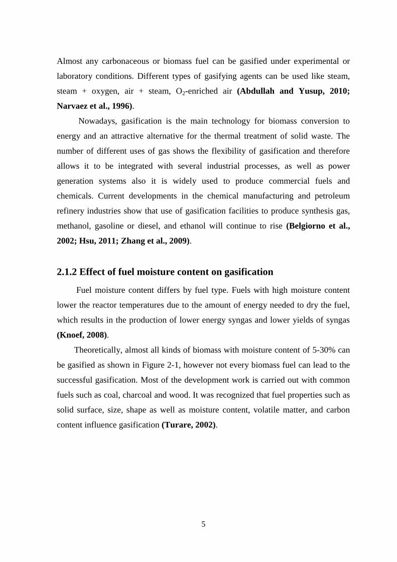
Almost any carbonaceous or biomass fuel can be gasified under experimental or
laboratory conditions. Different types of gasifying agents can be used like steam,
steam + oxygen, air + steam, O2-enriched air (Abdullah and Yusup, 2010;
Narvaez et al., 1996).
Nowadays, gasification is the main technology for biomass conversion to
energy and an attractive alternative for the thermal treatment of solid waste. The
number of different uses of gas shows the flexibility of gasification and therefore
allows it to be integrated with several industrial processes, as well as power
generation systems also it is widely used to produce commercial fuels and
chemicals. Current developments in the chemical manufacturing and petroleum
refinery industries show that use of gasification facilities to produce synthesis gas,
methanol, gasoline or diesel, and ethanol will continue to rise (Belgiorno et al.,
2002; Hsu, 2011; Zhang et al., 2009).
2.1.2 Effect of fuel moisture content on gasification
Fuel moisture content differs by fuel type. Fuels with high moisture content
lower the reactor temperatures due to the amount of energy needed to dry the fuel,
which results in the production of lower energy syngas and lower yields of syngas
(Knoef, 2008).
Theoretically, almost all kinds of biomass with moisture content of 5-30% can
be gasified as shown in Figure 2-1, however not every biomass fuel can lead to the
successful gasification. Most of the development work is carried out with common
fuels such as coal, charcoal and wood. It was recognized that fuel properties such as
solid surface, size, shape as well as moisture content, volatile matter, and carbon
content influence gasification (Turare, 2002).

6
2.2 Gasification Reactions
The chemistry of gasification is complex. The process of gasification
proceeds primarily via a two-step process, pyrolysis followed by gasification,
Figure 2-2. Pyrolysis is the decomposition of the biomass and/or coal feedstock by
heat. This step, also known as devolatilization, is endothermic and produces 75 to
90% volatile materials in the form of gaseous and liquid hydrocarbons. The
remaining nonvolatile material, containing high carbon content, is referred to as
char (Bridgwater and Evans, 1993).
Figure 2-2 Gasification Steps (Ciferno and Marano, 2002)
Figure 2-1 Moisture scale for gasification, (Turare, 2002).
Step 1
Pyrolysis
~500 oC
Gases
Liquids
Char
Step 2
Gasification
~1000 oC+
Syngas

7
The volatile hydrocarbons and char are subsequently converted to syngas in the
second step gasification. Reactions involved in this step are listed below:
1. Exothermic reactions, which involves the following reactions:
a. Combustion reactions producing CO2 and CO and release thermal energy,
which are both needed for gasification reactions. The combustion reactions
are faster than other gasification reactions and they occur first rapidly
consuming the oxygen, Table 2-1 (Basu, 2006).
b. Methanation and Shift conversion reactions, Table 2-1.
2. Endothermic reactions, these gasification reactions are water-gas reaction,
steam methane reforming reaction, and Boudouard reaction, Table 2-2.
Table 2-1 Gasification exothermic reactions (Heiskanen, 2011; Ciferno, and Marano,
2002)
Reactions Reaction heat , MJ/kmol Equation Number
Basic combustion reactions
-111 (1)
-283 (2)
-394 (3)
Methanation reaction
-75 (4)
Shift conversion
-41 (5)
Table 2-2 Gasification endothermic reactions (Heiskanen, 2011; Ciferno, and Marano,
2002)
Reactions Reaction heat, MJ/kmol Equation Number
Boudouard reaction
+172 (6)
8
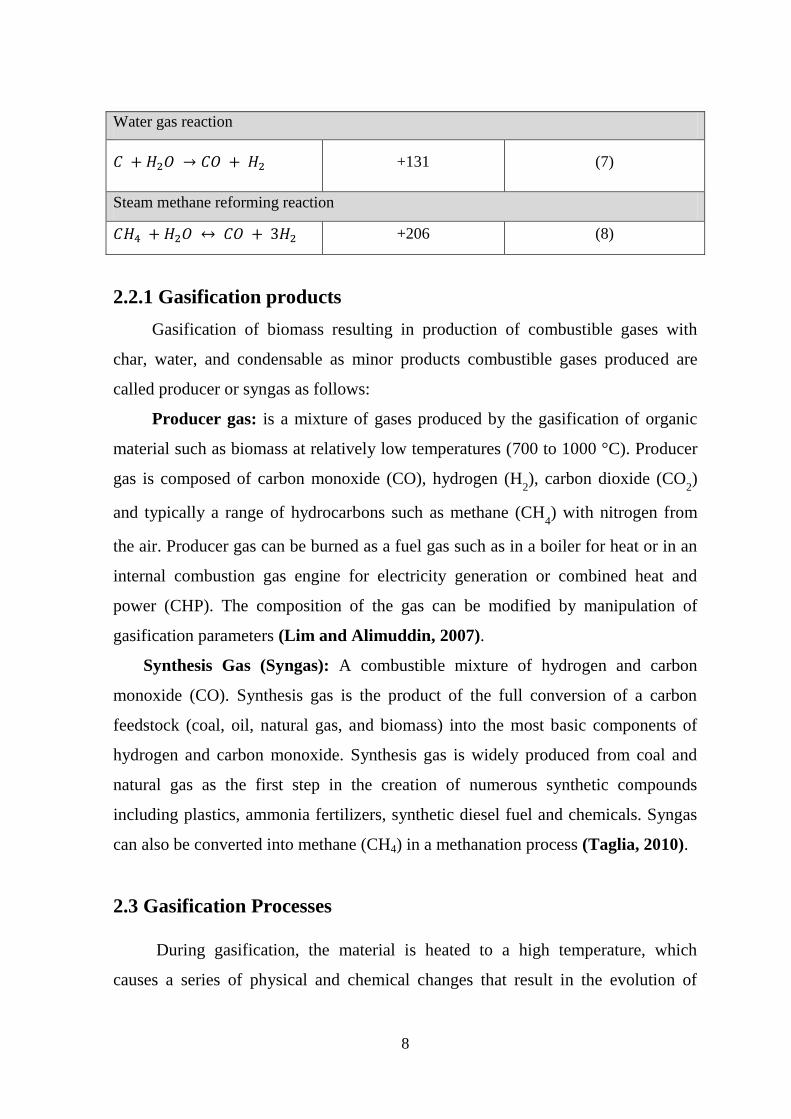
Water gas reaction
+131 (7)
Steam methane reforming reaction
+206 (8)
2.2.1 Gasification products
Gasification of biomass resulting in production of combustible gases with
char, water, and condensable as minor products combustible gases produced are
called producer or syngas as follows:
Producer gas: is a mixture of gases produced by the gasification of organic
material such as biomass at relatively low temperatures (700 to 1000 °C). Producer
gas is composed of carbon monoxide (CO), hydrogen (H2), carbon dioxide (CO
2)
and typically a range of hydrocarbons such as methane (CH4) with nitrogen from
the air. Producer gas can be burned as a fuel gas such as in a boiler for heat or in an
internal combustion gas engine for electricity generation or combined heat and
power (CHP). The composition of the gas can be modified by manipulation of
gasification parameters (Lim and Alimuddin, 2007).
Synthesis Gas (Syngas): A combustible mixture of hydrogen and carbon
monoxide (CO). Synthesis gas is the product of the full conversion of a carbon
feedstock (coal, oil, natural gas, and biomass) into the most basic components of
hydrogen and carbon monoxide. Synthesis gas is widely produced from coal and
natural gas as the first step in the creation of numerous synthetic compounds
including plastics, ammonia fertilizers, synthetic diesel fuel and chemicals. Syngas
can also be converted into methane (CH4) in a methanation process (Taglia, 2010).
2.3 Gasification Processes
During gasification, the material is heated to a high temperature, which
causes a series of physical and chemical changes that result in the evolution of

9
volatile products and carbonaceous solid residues. The gasification process uses an
agent, air, oxygen, hydrogen or steam to convert carbonaceous materials into
gaseous products (Basu, 2006).
2.3.1 Air gasification
Ergudenler, (1993) studied the effect of air flow rate on the gas quality and
quantity during air gasification of wheat straw in a fluidized bed gasifier. The
results showed that at equivalence ratio of 0.25, the mole fraction of the
combustible component achieved their maximum.
Cao et al., (2005) demonstrated a fluidized bed air gasification system using
sawdust. Two individual regions of pyrolysis, gasification, and combustion of
biomass combined in one reactor. The primary air stream and the biomass feedstock
were introduced into the gasifier from the bottom and the top, respectively.
Secondary air was injected into the upper region of the reactor to maintain elevated
temperature; the fuel gas was produced at a rate of about 3.0 Nm3/kg biomass and
heating value of about 5.0 MJ/Nm3. The concentration of hydrogen, carbon
monoxide and methane in the fuel gas produced were 9.27%, 9.25% and 4.21%,
respectively.
2.3.2 Steam gasification
Boateng et al., (1992) determined the effects of reactor temperature and steam
to biomass ratio on producer gas composition, heating value and energy recovery.
The produced gas, which is rich in hydrogen, had been found to have a heating
value ranging from 11.1 MJ/m3 at temperature of 700
oC to 12.1 MJ/m
3 at
temperature of 800oC. Energy recovery varied from 35-59% within the same
temperature range.
Mermoud et al., (2005) studied charcoal steam gasification of beech charcoal
spheres of different diameters 10-30 mm at different temperatures 830-1030 oC.
Results show a very slow reaction at 830 oC. A difference in gasification rate as
high 6.5 to 1 was observed between temperatures at 1030 and 830oC. Experiments
carried out with mixtures of H2O/N2 at 10%, 20%, and 40% mol of steam confirmed

10
that oxidant partial pressure influences gasification. A gasification rate of 1.9 was
obtained for H2O partial pressure varying from 0.4 to 0.1 atm.
2.3.3 Oxygen gasification
Tillman, (1987) gasified municipal solid waste in an oxygen gasifier. The
feedstock (shredded and magnetically sorted) was fed into the top of the gasifier and
the oxygen was fed at the bottom. Pyrolytic char was combusted with the oxygen at
the bottom of the gasifier providing enough thermal energy to produce temperatures
in the range of 1593-1704 oC and to produce a molten slag from all noncombustible
materials. The maximum mole fraction of the produced gas for CO, H2, CO2 and
CH4 recorded were 44%, 31%, 13% and 4%, respectively. The maximum heating
value was 10.6 MJ/Nm3.
2.3.4 Hydrogen gasification
Weil et al., (1978) used preheated hydrogen mixed with peat at the entrance
of fluidized bed gasifier. The reactor was operated as an entrained flow reactor in an
isothermal or a constant heat-up mode. Increasing the temperature from 426 oC to
760 oC increased carbon monoxide and hydrocarbon gases from 8% to 18% and
41% to 63%, respectively.
2.4 Gasification Reactors
Gasification reactors can be generally classified into two broad categories;
namely, fixed bed and fluidized bed. Fluidized bed gasifiers are more flexible in the
selection of fuel type. It can gasify various types of biomass without much difficulty
and has high carbon conversion rates as well as high heat transfer rates (Lim and
Alimuddin, 2007). Fluidized bed gasification performs better than fixed bed
gasification to reduce ash-related problems since the bed temperature of fluidized
bed gasification can be kept uniformly below the ash slagging temperature (Abdul
Salam et al, 2010).

11
2.4.1 Fixed Bed Gasifiers
The fixed bed gasification system consists of a reactor / gasifier with a gas
cooling and cleaning system. The fixed bed gasifier has a bed of solid fuel particles
through which the gasifying media and gas move either up or down. It is the
simplest type of gasifier consisting of usually a cylindrical space for fuel and
gasifying media with a fuel feeding unit, an ash removal unit and a gas exit. It is
made up of firebricks, steel or concrete. In the fixed bed gasifier the fuel bed moves
slowly down the reactor as the gasification occurs. The fixed bed gasifiers are of
simple construction and generally operate with high carbon conversion. There are
three basic fixed bed designs, Updraft, Downdraft and Cross-draft Gasifiers
(Chopra and Jain, 2007).
2.4.2 Fluidized Bed Gasifiers
A Fluidized Bed Gasifier has a bed made of an inert material (such as sand, ash
or char) that acts as a heat transfer medium. In this design, the bed is initially heated
and the fuel introduced when the temperature has reached the appropriate level. The
bed material transfers heat to the fuel and blows the reactive agent through a
distributor plate at a controlled rate. Unlike fixed bed gasifiers, fluidized bed
gasifiers have no distinct reaction zones and drying, pyrolysis, and gasification
occur simultaneously during mixing (Lim and Alimuddin, 2008).
The advantages of fluidize bed gasifiers are:
1. Strong gas-to-solids contact.
2. Excellent heat transfer characteristics.
3. Better temperature control.
4. Large heat storage capacity.
5. Good degree of turbulence.
6. High volumetric capacity.

12
The disadvantages are the large pressure drop, particle entrainment, and erosion
of the reactor body (Lettner et al., 2007).
2.4.2.1 Fluidize Bed Gasifiers Types
Fluidized Bed Gasifiers are classified by their configuration and the velocity
of the reactive agent. It consists of bubbling, circulating and spouted fluidized beds.
2.4.2.1.1 Bubbling Fluidized Bed Gasifier
In bubbling fluidized beds, granular material is fed into a vessel through which
an upward flow of gas passes at a flow rate where the pressure drop across the
particles is sufficient to support their weight (incipient fluidization). In bubbling
fluidization (at relatively low fluidization velocity just above the minimum
fluidization velocity), the gas in excess of that needed for minimum fluidization
passes through the bed in the form of bubbles. Bubbles grow by coalescence as they
rise in the bed. At the bed surface, the bubbles burst causing a shower of bed solids
to leave the bed surface and enter the freeboard, at which the carryover occurs.
Bubbling fluidized bed gasifiers (BFG) has potential for rural electrification
projects especially in third world countries where biomass supplies are abundant
from agricultural, wood industries and where electricity supply from the grid is not
available, Figure 2-3a (Lim and Alimuddin, 2008).
2.4.2.1.2 Circulating Fluidized Bed Gasifier
If the gas velocity in a bubbling fluidized bed is further increased, more
particles will be entrained in the gas stream and leave the reactor. Eventually the
transport velocity for most of the particles is reached, and the vessel can be quickly
emptied of solids unless additional particles are fed to the base of the reactor. If the
solids leaving the vessel are returned through an external collection system, the
system is called a circulating or fast fluidized bed (CFB) system. The streams of

13
particles moving upward in the reactor are at solid concentrations well above that
for dilute phase transport. Compared to conventional furnaces, circulating beds have
a higher processing capacity, better gas-solid contact, and the ability to handle
cohesive solids that might otherwise be difficult to fluidize in bubbling fluidized
beds. Despite these advantages, circulating fluidized beds are still less commonly
used that bubbling models, primarily because their height restricts their applications
in terms of cost analysis, Figure 2-3b (Brown, 2006).
Figure 2-3 Fluidised Bed Gasifiers; a: Bubbling Fluidized Bed Gasifier; b: Circulating
Fluidized Bed Gasifier; c: Spouting Fluidized Bed Gasifier; and d: Gas Indirect Gasifier
(Craig and Margaret, 1996).
Fuel hoppers
Air
Heater
a b
c d
14
2.4.2.1.3 Spouted Fluidized Bed Gasifier
The bed is filled with relatively coarse particulate solids, Geldart group D.
Fluid is injected vertically through a centrally located small opening at the base of
the vessel. If the fluid injection rate is high enough, the resulting high velocity jet
causes a stream of particles to rise rapidly in a hollowed central core within the bed
of solids. These particles, after reaching somewhat above the peripheral bed level,
rain back onto the annular region between the hollowed core and the column wall,
where they slowly travel downward and, to some extent, inward as a loosely packed
bed. As the fluid travels upward, it flares out into the annulus. The overall bed
thereby becomes a composite of a dilute phase central core with upward moving
solids entrained by a concurrent flow of fluid and a dense phase annular region with
counter region with counter-current percolation of the fluid. The central core is
called a spout and the peripheral annular region is referred to as the annulus. The
term fountain denotes the mushroom-shaped zone above the level of the annulus. To
enhance motions of the solids and eliminate dead spaces at the bottom of the vessel,
it is common to use a diverging conical base with fluid injection at the truncated
apex of the cone, Figure 2-3c (Hoque and Bhattacharya, 2001; Thamavithya et
al., 2010). Spout-Fluid Beds have been of increasing interest in the petrochemical,
chemical and metallurgic industries since spout-fluid beds can reduce some of the
limitations of both spouting and fluidization by superimposing the two type of
system (Zhong, 2005).
2.4.3 Indirect Fluidized Bed Gasifier
Indirect gasifiers are the reactors used for the steam indirect gasification and
are grouped as char indirect gasifiers and gas indirect gasifiers depending on the
type of internal energy source. The main advantage of indirect gasification is the
high quality of the combustible gas produced in contrast with greater investment
and maintenance cost of the reactor. Therefore it is necessary to improve the quality

15
of gas with the adoption of a highly efficient energy recovery system, Figure 2-3d
(Craig and Margaret, 1996).
2.5 Geldart Classification of Particles
Geldart (1973) observed the nature of particles fluidizing. He categorized his
observations by particle diameter versus the relative density difference between the
fluid phase and the solid particles. Geldart identified four regions in which the
fluidization character can be distinctly defined, Figure 2-4.
Group A Small particle size or density less than 1.4 g/cm3. Easily fluidized
with smooth fluidization at low gas velocities and controlled bubbling with small
bubbles at higher gas velocities. When fluidized by air at ambient conditions, result
in a region of non-bubbling fluidization beginning at Umf, followed by bubbling
fluidization as fluidizing velocity increases. Gas bubbles rise faster than the rest of
the gas.
Group B Are sand like powders which result in vigorous bubbling fluidization
under these conditions. Bubbles form as soon as the gas velocity exceeds the
minimum fluidization velocity. Majority of gas-solid reactions occur in this regime
based on particle size of raw materials.
Group C Cohesive or very fine powders. Normal fluidization is difficult for
these solids because of interparticle forces that are greater than those resulting from
the action of the gas on the particles. In small diameter beds these particles form a
plug of solids that rises upward. Powders, very fine, cohesive powders which are
incapable of fluidization in the strict sense. Examples: Face powder, flour, and
starch.
Group D Spoutable, large and/or dense particles. Examples include drying
grains, peas, roasting coffee beans, gasifying coals and roasting of metal ores
(Yang, 2006).

16
Figure 2-4 Geldart classification of particles according to fluidization properties (Yang,
2006).
2.6 Characteristics of Spouted Fluidized Bed
2.6.1 The phenomena of Fluidization
The fluidization principle was first used on an industrial scale in 1922 for the
gasification of fine-grained coal. Since then, fluidized beds have been applied in
many industrially important processes (Werther, 2012).
Different parameters influence the fluidization characteristics and they can be
classified into two major groups comprised of independent variables and
dependent variables. Independent variables include fluid properties (e.g.,
density, viscosity, relative humidity), particle characteristics (e.g., density, size,
shape, distribution, surface roughness, and porosity) and equipment related such as
direction of fluid flow, distributor plate design, vessel geometry, operating velocity,
centrifugal force, temperature, pressure, type of nozzle, etc. The dependent
variables are basically capillary forces, minimum fluidization velocity, electrostatic
forces, bed voltage; Vander Waals forces (Dixit and Shivanand, 2009).
In fluidization an initially stationary bed of solid particles is brought to a
―fluidized‖ state by an upward stream of gas or liquid as soon as the volume flow
rate of the fluid exceeds a certain limiting value Umf (where mf denotes minimum
fluidization). In the fluidized bed, the particles are held suspended by the fluid

17
stream; the pressure drop Δpfb of the fluid on passing through the fluidized bed is
equal to the weight of the solids minus the buoyancy, divided by the cross sectional
area Ac of the fluidized-bed vessel, Figure 2-5.
( ) ( )
(2.1)
In Equation (2.1), the porosity ε of the fluidized bed is the void volume of the
fluidized bed (volume in interstices between grains, not including any pore volume
in the interior of the particles) divided by the total bed volume; is the solids
apparent density; and H is the height of the fluidized bed (Werther, 2012).
Figure 2-5 Pressure drop in flow through packed and fluidized beds (Werther, 2012).
2.6.2 Minimum fluidization velocity
A minimum velocity is needed to fluidize a bed. If the velocity is too small the
bed stays fixed and operates as a packed bed. In spout fluidized beds the favourable
properties of both spouted and fluidized beds are combined. Schematic diagram is
shown in Figure 2-6. Table 2-3 shows correlations proposed by previous authors for
Umf.

18
Figure 2-6 Schematic draw of spouted bed (Smith et al., 1981); (Abdul Salam and
Bhattacharya, 2006)
Table 2-3 Correlations for and
Reference Equations Equation
No.
Jackson and
Judd,
(1981)
,. /
-
Where:
( )
(2.2)
Littman et
al., (1981)
( )
[{ ( )
( ) }
]
Where:
( )
(2.3)
Thonglimp
et al., (1984)
( ) ( )
(2.4)
Gasification agent
Annulus
Distributer
Cylindrical column
Conical section
Spout
Fountain

19
Wen and
Yu, (1966)
√
Where:
(
)
Constants C1 and C2 shown in Table 2-4
(2.5)
Table 2-4 Parameters used in Wen and Yu type equations for minimum fluidization
velocity (Abdul Salam and Bhattacharya, 2006)
Reference
Equation parameters
C1 C2
Bourgeoisand Grenier,
(1968) 25.46 0.0384
Grace, (1982) 27.2 0.0408
Thonglimp et al., (1984) 31.6 0.0425
Lucas et al., (1986) 29.5 0.0357
Tannous, (1993) 25.83 0.0430
2.6.3 Minimum spouting velocity (Ums)
The minimum fluid velocity at which a bed will remain in the spouted state,
defined as the minimum spouting velocity (Ums), depends on solid and fluid
properties on one hand and bed geometry on the other. Data on minimum spouting
velocity in packed beds as described in literature are scarce. The minimum spouting
velocity is measured experimentally by first achieving a spout regime and then
decreasing the gas velocity slowly until the spout is no longer permanent, the
porosity at that instant will be larger than that for a fixed bed. So, at that instant,
when measurements of minimum spouting velocity are made, the porosity of bed is
certainly higher than the porosity reported for the fixed bed (Dogan et al., 2004).
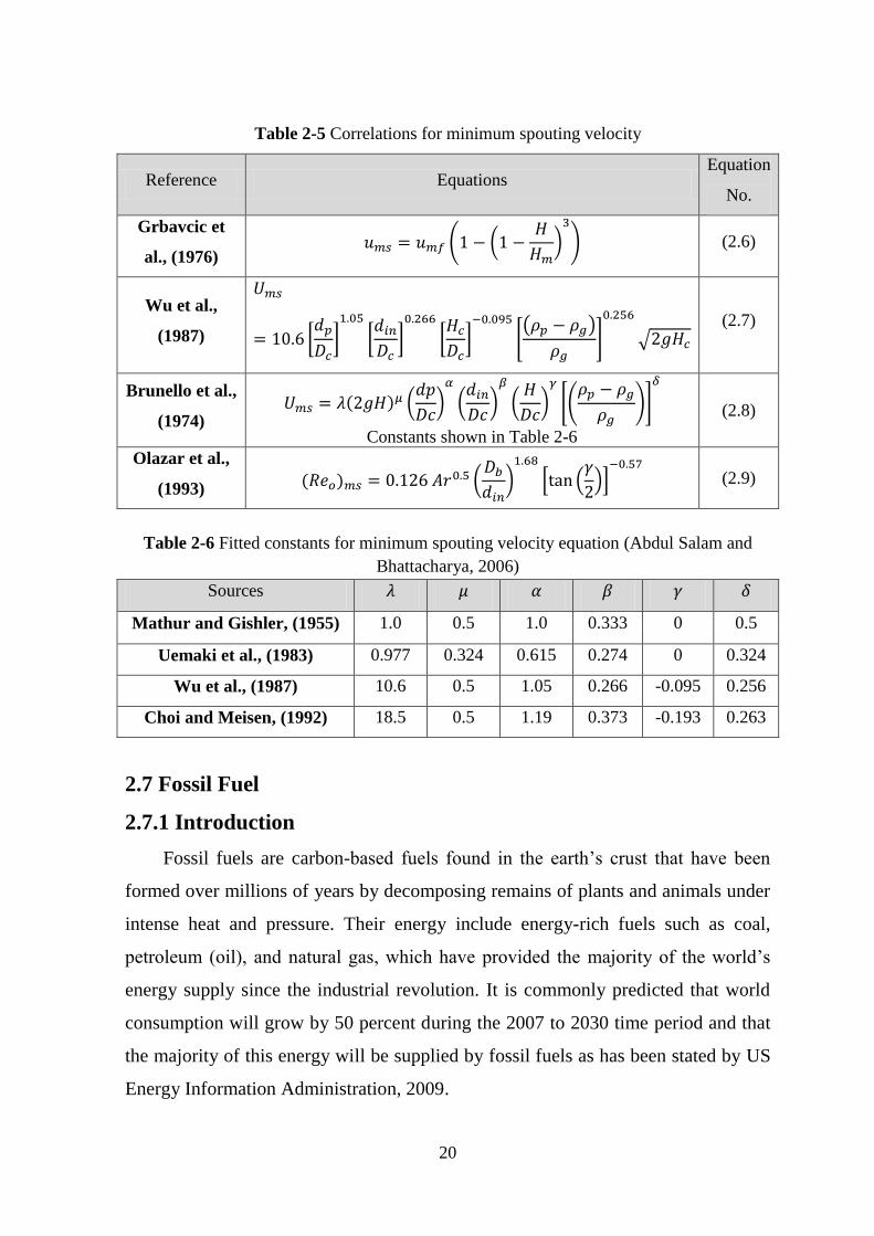
Tables 2-5 and 2-6 list correlations of Ums proposed by different authors.
20
Table 2-5 Correlations for minimum spouting velocity
Reference Equations Equation
No.
Grbavcic et
al., (1976) ( (
)
) (2.6)
Wu et al.,
(1987)
[
]
[ ]
[ ]
*( )
+
√ (2.7)
Brunello et al.,
(1974) ( )
(
)
( )
(
)
*(
)+
Constants shown in Table 2-6
(2.8)
Olazar et al.,
(1993) ( )
( )
0 .
/1
(2.9)
Table 2-6 Fitted constants for minimum spouting velocity equation (Abdul Salam and
Bhattacharya, 2006)
Sources
Mathur and Gishler, (1955) 1.0 0.5 1.0 0.333 0 0.5
Uemaki et al., (1983) 0.977 0.324 0.615 0.274 0 0.324
Wu et al., (1987) 10.6 0.5 1.05 0.266 -0.095 0.256
Choi and Meisen, (1992) 18.5 0.5 1.19 0.373 -0.193 0.263
2.7 Fossil Fuel
2.7.1 Introduction
Fossil fuels are carbon-based fuels found in the earth‘s crust that have been
formed over millions of years by decomposing remains of plants and animals under
intense heat and pressure. Their energy include energy-rich fuels such as coal,
petroleum (oil), and natural gas, which have provided the majority of the world‘s
energy supply since the industrial revolution. It is commonly predicted that world
consumption will grow by 50 percent during the 2007 to 2030 time period and that
the majority of this energy will be supplied by fossil fuels as has been stated by US
Energy Information Administration, 2009.

21
The recent increase in fossil fuel prices and worsening effects of global
warming has prompted the use of biomass as a source of energy. Unlike other
renewable energy sources that require costly technology, biomass can generate
electricity with the same type of equipment and power plants that now burn fossil
fuels. However low thermal efficiencies have hindered its development and the
main challenge now is to develop low cost high efficiency systems. In 2007,
approximately 86 percent of world energy production came from burning fossil
fuels. The majority of fossil fuels are used in the electric-power generation,
transportation, manufacturing and residential heating industries (Lim and
Alimuddin, 2008).
2.7.2 Coal
Coal is a fossil fuel created from the remains of plants that lived and died about
100 to 400 million years ago when parts of the Earth were covered with huge
swampy forests. Coal is classified as a non-renewable energy source because it
takes millions of years to form. The energy we get from coal today comes from the
energy that plants absorbed from the sun millions of years ago. All living plants
store solar energy through a process known as photosynthesis. When plants die, this
energy is usually released as the plants decay. Under conditions favourable to coal
formation, however, the decay process is interrupted, preventing the release of the
stored solar energy. The energy is locked into the coal. Millions of years ago, dead
plant matter fell into swampy water and over the years, a thick layer of dead plants
lay decaying at the bottom of the swamps. Over time, the surface and climate of the
Earth changed, and more water and dirt washed in, halting the decay process. The
weight of the top layers of water and dirt packed down the lower layers of plant
matter. Under heat and pressure, this plant matter underwent chemical and physical
changes, pushing out oxygen and leaving rich hydrocarbon deposits. What once had
been plants gradually turned into coal (Secondary and Intermediate Energy
ebooks, 2011).

22
2.7.2.1 Coal production
The world currently consumes over 4000 million tons coal each year. The
largest consumers are mainly power generation and steel industry. Cement
manufacturing and coal liquefaction are two a medium consumers. A small
proportion of coal is also used for various chemical processes. Coal production has
increased with 38% the last 20 years. Asia is the fastest growing coal producer,
while European production actually has declined. Global coal production is
expected to reach 7 billion tonnes in 2030 with China accounting for nearly half the
increase. Coal still plays a vital role in the world‘s primary energy mix, providing
23.5% of global primary energy needs in 2002, 39% of the world‘s electricity, more
than double the next largest source, and an essential input into 64% of the world‘s
steel production (Höök, 2007).
Figure 2-7 Coal consumed for electricity (Höök, 2007).
2.8 Biomass
2.8.1 Introduction
Biomass is a renewable energy source whose advantages and drawbacks,
compared to fossil fuels, are periodically analysed (Goldemberg, 2004). Biomass is
an umbrella term used to describe vegetable or animal (biological) sourced energy
mass, for example canola and lard. Biomass fuels may be derived from many

23
sources, including forestry products and residue, agriculture residues, food
processing wastes, and municipal and urban wastes (Roos, 2008).
2.8.2 Biomass algae
Algae have recently received a lot of attention as a new biomass source for the
production of renewable energy. Some of the main characteristics which set algae
apart from other biomass sources are that algae can have a high biomass yield per
unit of light and area, can have a high oil or starch content (Global bioenergy
partnership, 2009).
Algae range from small, single-celled organisms to multi-cellular organisms,
some with fairly complex and differentiated form. Algae are usually found in damp
places or bodies of water and thus are common in terrestrial as well as aquatic
environments. Like plants, algae require primarily three components to grow:
sunlight, carbon-dioxide and water. Photosynthesis is an important bio-chemical
process in which plants, algae, and some bacteria convert the energy of sunlight to
chemical energy (Wagner, 2007; Wen and Michael, 2009).
Algae biomass has the potential to grow yields far higher than any other
feedstock currently being used. It has the possibility of a much higher energy yield
per unit, so it can be much more efficient (Campbell, 2008).
Figure 2-8 Oil Yields of Feedstocks for Biofuel from EarthTrends (Global bioenergy
partnership, 2009).

24
Algal concentration may vary substantially from sample to sample. The
variability can be attributed to spatiotemporal variability of the collection, as well as
variability in the processing, storage, and analysis of the sample (Berkman and
Michael, 2007).
2.8.3 Types of Algae There are two classifications of algae: macroalgae and microalgae.
2.8.3.1 Macro-algae
Seaweeds or macro-algae belong to the lower plants, meaning that they do not
have roots, stems and leaves. Instead they are composed of a thallus (leaf-like) and
sometimes a stem and a foot. Some species have gas-filled structures to provide
buoyancy. The big advantage of macro-algae is their huge mass production
(Carlsson et al., 2007).
2.8.3.2 Micro-algae
Micro-algae are microscopic photosynthetic organisms that are found in both
marine and freshwater environments. Their photosynthetic mechanism is similar to
land based plants, but due to a simple cellular structure, and submerged in an
aqueous environment where they have efficient access to water, CO2 and other
nutrients, they are generally more efficient in converting solar energy into biomass
(Wagner, 2007).
The technical potential of macro- and micro-algae for biomass production and
greenhouse gas abatement has been recognised for many years, given their ability to
use carbon dioxide and the possibility of their achieving higher productivities than
land-based crops (Wellinger, 2009).
Macro- and micro-algae are currently mainly used for food, in animal feed, in
feed for aquaculture and as bio-fertiliser. Biomass from micro-algae is dried and
marketed in the human health food market in form of powders or pressed in the
form of tablets (Wen and Michael, 2009).

25
2.9 Hydrogen
Hydrogen is well known. It is the smallest of all atoms. Promoters praise the
energy content of hydrogen. In the past, many have considered the production and
use of hydrogen, assuming that it is just another gaseous fuel and can be handled
much like natural gas in today‘s energy economy (Eliasson and Taylor, 2005).
2.9.1 Hydrogen Production methods
2.9.1.1 Coal gasification
Hydrogen can be produced from coal through a variety of gasification
processes (e.g. fixed bed fluidized bed or entrained flow). In practice, high-
temperature entrained flow processes are favored to maximize carbon conversion to
gas, thus avoiding the formation of significant amounts of char, tars and phenols. A
typical reaction for the process is given in the following equation, in which carbon
is converted to carbon monoxide and hydrogen.
C(s) + H2O + heat CO + H2 (9)
Purdy et al. (1984) made experimental work to gasify New Mexico
subbituminous coal with steam and oxygen in a 15.2 cm inside diameter fluidized
bed reactor at a pressure of 790 kPa (100 psig) and average bed temperatures
between 875 and 990 oC. Material balances were obtained on total mass and major
elements (C, H, 0, N, S). A simple representation of coal pyrolysis has been added
to a previously developed model of gasification and combustion; the resulting
model provides good correlations of measured carbon conversions, make gas
production rates, and make gas compositions. Approximations that can be used to
estimate sulfur conversion and the split between H, S and COS in the product gas
have also been developed.
Neogi et al., (1986) used a bench-scale fluidized bed reactor for the
gasification of coal with steam as the fluidizing medium. A mixture of sand and
limestone used as the bed material made it possible to gasify a caking coal without
the problem of agglomeration. The gas composition and yield of the hydrogen-rich
26
product gas were studied as a function of temperature. A mathematical model was
developed to study the heterogeneous reactions taking place in the reactor and also
the transient behaviour of the system.
Chatterjee, (1995) studied gasification of high ash India coal in a laboratory-
scale, atmospheric fluidized bed gasifier using steam and air as fluidizing media. A
one-dimensional analysis of the gasification process has been presented
incorporating a two-phase theory of fluidization, char gasification, volatile release
and an overall system energy balance. Results are presented on the variation of
product gas composition, bed temperature, calorific value and carbon conversion
with oxygen and steam feed. Comparison between predicted and experimental data
has been presented, and the predictions show similar trends as in the experiments.
Zedtwitz and Steinfeld, (2005) studied the steam-gasification of coal in a
fluidized-bed or a packed-bed chemical reactor using an external source of
concentrated thermal radiation for high-temperature process heat. The authors found
that above 1450 K, the product composition consisted mainly of an equimolar
mixture of H2 and CO, a syngas quality that is notably superior than that typically
obtained in autothermal gasification reactors (with internal combustion of coal for
process heat), besides the additional benefit of the upgraded calorific value.
Jin, et al., (2010) applied a supercritical water gasification system with a
fluidized bed reactor to investigate the gasification of coal in supercritical water. 24
wt% coal- water- slurry was continuously transported and stably gasified without
plugging problems; a hydrogen yield of 32.26 mol/kg was obtained and the
hydrogen fraction was 69.78%. The effects of operational parameters upon the
gasification characteristics were investigated.
2.9.2. Biomass Sources
Lv et al., (2002) investigated the characteristics of biomass air-steam
gasification in a fluidized bed for hydrogen-rich gas production through a series of
experiments. The effects of reactor temperature, steam-to-biomass ratio,

27
equivalence ratio ER, and the biomass particle size on gas composition and
hydrogen production were investigated. The authors concluded that the higher
reactor temperature, the proper ER, proper steam-to-biomass ratio S/B, and smaller
biomass particle size will contribute to more hydrogen production. The highest
hydrogen yield, 71g H2/ kg biomass (wet basis), was achieved at a reactor
temperature of 900 °C, S/B of 2.70. It was also shown that under proper operating
parameters biomass air-steam gasification in a fluidized bed was one effective way
for hydrogen-rich gas production.
Kong et al., (2008) found that hydrothermal gasification of biomass wastes
can be identified as a possible system for producing hydrogen. The authors
investigated the decomposition of biomass, as a basis of hydrothermal treatment of
organic wastes. To eliminate chars and tars formation and obtain higher yields of
hydrogen, catalyzed hydrothermal gasification of biomass wastes was summarized.
González et al., (2008) studied the production of hydrogen-rich gas by
air/steam and air gasification of olive oil waste was investigated. The study was
carried out in a laboratory reactor at atmospheric pressure over a temperature range
of 700-900°C using a steam/biomass ratio of 1.2 w/w. The solid, energy and carbon
yield (%), gas molar composition and high heating value of the gas (kJ NL−1
), were
determined for all cases and the differences between the gasification process with
and without steam were established. The results obtained suggest that the operating
conditions were optimized at 900°C in steam gasification (a hydrogen molar
fraction of 0.70 was obtained at a residence time of 7 min). The use of both
catalysts ZnCl2 and dolomite resulted positive at 800 °C, especially in the case of
ZnCl2 (attaining H2 molar fraction of 0.69 at a residence time of 5 min).
28
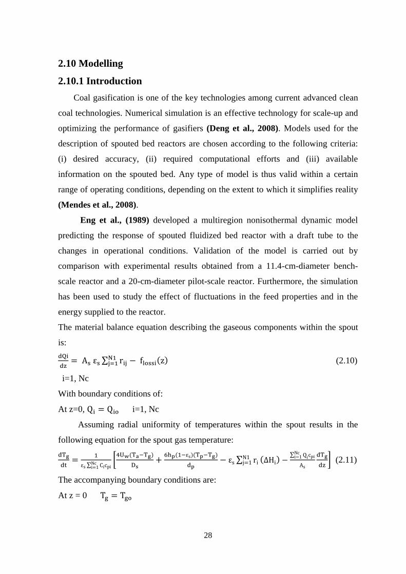
2.10 Modelling
2.10.1 Introduction
Coal gasification is one of the key technologies among current advanced clean
coal technologies. Numerical simulation is an effective technology for scale-up and
optimizing the performance of gasifiers (Deng et al., 2008). Models used for the
description of spouted bed reactors are chosen according to the following criteria:
(i) desired accuracy, (ii) required computational efforts and (iii) available
information on the spouted bed. Any type of model is thus valid within a certain
range of operating conditions, depending on the extent to which it simplifies reality
(Mendes et al., 2008).
Eng et al., (1989) developed a multiregion nonisothermal dynamic model
predicting the response of spouted fluidized bed reactor with a draft tube to the
changes in operational conditions. Validation of the model is carried out by
comparison with experimental results obtained from a 11.4-cm-diameter bench-
scale reactor and a 20-cm-diameter pilot-scale reactor. Furthermore, the simulation
has been used to study the effect of fluctuations in the feed properties and in the
energy supplied to the reactor.
The material balance equation describing the gaseous components within the spout
is:
∑
( ) (2.10)
i=1, Nc
With boundary conditions of:
At z=0, i=1, Nc
Assuming radial uniformity of temperatures within the spout results in the
following equation for the spout gas temperature:
∑
[ ( )
( )( )
∑
( )
∑
] (2.11)
The accompanying boundary conditions are:
At z = 0

29
At t = 0 ( ) ( )
A similar energy balance for the spout particles yields the following expression for
the spout particle temperature:
( )
(
)
( )
( )
( ) (2.12)
The boundary conditions associated with this PDE are:
At z=0 Tp = Tao
At t=0 Tp(z)= Tpo(z)
Responses of spout gas temperature profiles are found to exhibit two trends.
First, a sudden pseudo steady state is found to appear with a time constant
comparable to the residence time of the reacting gases (e.g., 30 ms). Second, long-
term responses are found to be dependent upon the dynamics of the annular
temperature (e.g., 15 min). Simulations of dynamic responses for various
disturbances indicate that short-term dynamic behavior is strongly affected by
changes in the inlet gas stream properties. Long-term responses, however, are
dependent upon the dynamics of the annular temperature.
Lucas et al., (1998) developed a two-region model of a spouted bed gasifier,
the model assumes first-order reaction kinetics for the gasification reactions and the
spout is treated as a plug flow reactor of fixed diameter with cross flow of gas into
the annulus. The annulus region is considered to be a single plug flow reactor.
Solids move in plug flow in both annulus and spout, independent of temperature
and reaction. The model allows predictions of axial profiles of temperature and gas
in the spout and annulus as well as exit gas compositions and overall carbon
conversion.
In a given increment of spout height the pyrolysis and char gases are added
to the gases from the previous increment in a manner that ensures that the
generation is largest at the spout entrance and decreases with spout height. This
pattern is achieved by the following equation:
( )
( ) ∫ [ .
/
]
(2.13)

30
The gas flow and gas compositions entering annulus section j are, respectively:
(2.14)
(2.15)
The authors predicted an equation to calculate the average temperature at the
gasifier exit:
∑
( )
∑ (
)
(
)∑
(2.16)
For ease of computation, the number of streamtubes was reduced to one. Predicted
axial composition profiles in the annulus were affected more by the reduction in the
number of streamtubes than by the change from isothermal to nonisothermal
conditions. The axial profile was shown to depend strongly on the assumed solids
recirculation rates. Comparisons made between predicted axial temperature profiles
and those measured in a pilot gasifier showed good agreement for both air
gasification of a highly reactive sub-bituminous coal and oxygen gasification of a
much less reactive anthracite. In the lower spout region where heat losses were
large, agreement was poorer.
Mendes et al., (2008) modelled a spouted bed reactor operating at high
temperature through one dimensional model in which heat transfer has been
carefully described at different levels of complexity. The process of coal
gasification has been selected to demonstrate the models achievements and
predictions have been compared to previous spouted bed reactor experimental
results. The authors studied the velocity of particles in the spouted bed and they
predicted an equation to calculate the velocity of the solid articles in the annular:
( )
(2.17)
The conservation equations for the gaseous component j in the spout and annulus
were predicted by the authors as follows:
Spout region:
(2.18)

31
Annulus region:
0
1 ( ) (2.19)
Two types of one-dimensional spouted bed reactor models are presented: a pseudo
homogeneous model and a heterogeneous one. In the pseudo homogeneous
approach, energy balances are function of a unique temperature characteristic of the
flow region and representative of both gas and solid phases.
Pseudo homogeneous approach, spout region:
[ ]
0
1 ( ) ∑( ) (2.20)
Pseudo homogeneous approach, annulus region:
( )
.
/ ( )
∑( ) ( ) (2.21)
In the heterogeneous approach, four energy balances are written, which correspond
to gas and particle temperature fields in each hydrodynamic region of the bed.
Heterogeneous approach, spout region:
Gas phase:
( )
[ ] ∑( ) (2.22)
Solid phase:
( )
[ ] 0
1 (
) ∑( ) (2.23)
Heterogeneous approach, annulus region:
Gas phase:
( )
[ ] 0
1 ( ) ∑( ) (2.24)
Solid phase:
( )
[ ]
( ) ∑( ) (2.25)
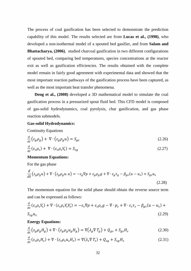
32
The process of coal gasification has been selected to demonstrate the prediction
capability of this model. The results selected are from Lucas et al., (1998), who
developed a non-isothermal model of a spouted bed gasifier, and from Salam and
Bhattacharya, (2006), studied charcoal gasification in two different configurations
of spouted bed, comparing bed temperatures, species concentrations at the reactor
exit as well as gasification efficiencies. The results obtained with the complete
model remain in fairly good agreement with experimental data and showed that the
most important reaction pathways of the gasification process have been captured, as
well as the most important heat transfer phenomena.
Deng et al., (2008) developed a 3D mathematical model to simulate the coal
gasification process in a pressurized spout fluid bed. This CFD model is composed
of gas-solid hydrodynamics, coal pyrolysis, char gasification, and gas phase
reaction submodels.
Gas-solid Hydrodynamics:
Continuity Equations
( ) ( ) (2.26)
( ) ( ) (2.27)
Momentum Equations:
For the gas phase
( ) ( ) ( )
(2.28)
The momentum equation for the solid phase should obtain the reverse source term
and can be expressed as follows:
( ) ( ) ( )
(2.29)
Energy Equations:
( ) ( ) ( ) (2.30)
( ) ( ) ( ) (2.31)

33
The heat exchange between phases can be expressed as a function of the
temperature difference and conform to the local balance condition
(2.32)
( ) (2.33)
The simulation results of the outlet molar fraction of gas composition are expressed
by the area average as below:
∫ (2.34)
The authors found that the prediction results are in good agreement with the
experimental data. Most of the calculation errors are within the range of 10%. In
addition they concluded that CFD modeling can be used for complex fluidized beds
coal gasification processes.

34
Chapter Three
Theoretical Modeling
3.1 Simulation of gas – solid system model
3.1.1 Steady – State model assumptions
1. Mass transfer by flow occurs in z direction by the stream of gasification
agent (air + steam) which passes from the bottom to the top of the gasifier.
2. Mass transfer between gas bulk and particle occurs by diffusion and by
convection (bulk flow) in both axial direction (z) and radial direction (r).
3. Close to the particle boundary, mass transfer occurs solely by diffusion
through the boundary layer surrounding the solid particles, from the bulk to
the surface of the solid particle due to the concentration difference for the
reacted species presented in the gas.
4. The reaction occurs on the surface of the solid particle consuming the carbon
in the solid fuel and the produced species, which is in gas phase, leave the
surface of the solid particle after the reaction has been completed.
3.2 Steady – state model equations
Modeling equations consist of mass balance equations for the gas – phase in
the bulk gas and on the surface of the solid particles.
3.2.1 Mass balance to obtain the continuity equation in the gas phase
Figure 3-1 shows a schematic diagram of the fluidized bed. Mass balance was
carried out over a differential element (Figure 3-1b), in the gas bulk of gasifier. This
differential element is a hollow cylindrical shape consists of solid particles.

35
Figure 3-1 Schematic sketch for the gasifer and the gas cell taken to make the balance
The following inventory rate equation can be written to describe the
transformation of the particular conserved quantity of component i, (Tosun, 2002):
[(Rate of mass In) – (Rate of mass out)]by flow + [(Rate of mass In) – (Rate of
mass out)]by molecular diffusion + Generation = Consumption + Accumulation (3.1)
The gas enters the gasifier from the bottom and flows in z – direction; therefore
there is mass transfer by bulk flow (convection) in z – direction. In addition due to
the concentration gradient in z and r direction, mass transfer occurs by molecular
diffusion as well. The detailed steps for the balance are shown as follows:
z – direction
Where:
Q: Volumetric gas flow rate
U: Superficial gas velocity
A: Cross sectional area of the element
u: Interstitial gas velocity
Solid – phase
Gas – phase
Spout
region
Annulus
regions
a
∆z
∆r
Differential
element
b

36
: Porosity of the bed,
( ) , (Darby, 2001)
(3.2)
(
) (3.3)
(3.4)
( ) (
) ( ) (3.5)
(No reaction will occur in the gas – phase).
r – direction
(3.6)
( )
(
) ( ) (3.7)
.
/
Where:
( – ) ,( ) - hence,
.
/ (3.8)
Substitute Equations. (3.2), (3.3), (3.4), (3.5), (3.6), (3.7), and (3.8) into equation
(3.1):
*,( ) (
)- + * (
) ( ) + * (
) (
) + .
/ (3.9)
Rearrange the above equation:
.
/ (3.10)
Divide equation (3.10) by
.
/ (3.11)

37
From Fick‘s first law, the mass flux (Kreith and Boehm, 1999) can be written
as:
,
Where:
De: is the diffusivity of gas and the subscript e denotes an effective diffusivity that
accounts for the presence of the solid material (Geankoplise, 1998).
Substitute for Niz and Nir into equation (3.11):
.
/
.
/
.
/ .
/
(Limtrakul, 2003)
So equation above can be written as follows:
.
/
.
/
.
/
.
/ (3.12)
Boundary conditions:
.
/
.
/
.
/
Equation (3.12) represents the general continuity equation for the gas – phase
species in the bulk.
The spouted bed consists of two regions; spout and annulus regions, Figure
(3-1). The spout region lies at the centre of the gasifier and the annulus regions lie
around the spout. So, equation (3.12) can be written for the two regions, spout and
annulus.
3.2.2 Gas – phase equations for the spout and annulus regions
a- Spout region
Equation (3.12) can be written for the gas – phase at the spout region:

38
.
/
.
/
.
/
.
/ (3.13)
At steady – state .
/
So, equation (3.13) becomes:
.
/
.
/
.
/
(3.14)
Re-arrange equation (3.14):
.
/
.
/
.
/
.
/ (3.15)
Equation (3.15) can be used to calculate the concentration profile of the gas –
phase species in the spout region. The diameter of the spout is calculated in
Appendix (D.1) and it is equal to 0.04 m. So, the annulus equivalent diameter is the
difference between the column diameter and the spout diameter:
Annulus equivalent diameter = column diameter – spout diameter
Annulus equivalent diameter = (0.077 – 0.04) m = 0.037 m.
The space of annulus on each side will be 0.037/2 = 0.0185 m
The velocity in equation (3.15) is the gas – phase velocity at the spout, and
the porosity represents the bed porosity at the spout region which are calculated in
Appendix (D.2) and (D.3) respectively.
Figure 3-2 shows the diameter of the spout and the annulus space on each side of
the gasifier.

39
Figure 3-2 Schematic diagram of the spout fluidized bed gasifier
b- Annulus region
The voidage in the annulus ɛa is usually close to the minimum fluidization
condition (Lim, et al., 1991; Sanchez et al., 2000):
For the concentration of the gas – phase species at the annulus, equation (3.12)
can be arranged as follows:
.
/
.
/
.
/
(3.16)
The velocity in equation (3.16) represents the gas – phase velocity in the annulus
region and it is calculated in Appendix (D.4).
0.032085 m
Dc = 0.077 m
Ds = 0.04 m
0.0185 m 0.0185 m
0.065
m
0.006415
m

40
(3.17)
Equation (3.17) represents the concentration and velocity profile of the gas – phase
at the annulus region.
3.2.3 Gas – Solid interface
The gas species diffuses from the bulk with concentration of Cib to the surface
of the solid particle through the boundary layer surrounding the particle by
molecular diffusion and then reacts on the surface of the particle. The gas
concentration on the solid fuel surface is Cis.
The solid particle is surrounded by a boundary layer which is defined as the
distance from a solid surface to a position where the concentration of the diffusing
species reaches 99% of the bulk concentration. All the resistance to mass transfer is
found within this hypothetical stagnant film and the properties (i.e., concentration,
temperature) of the fluid at the outer edge of the film are identical to those of the
bulk fluid (Fogler, 1999; Geankoplise 1998). Calculation of boundary layer
thickness can be shown in Appendix (D.5).
A differential element of thickness = ∆r in the boundary layer was taken and a
mass balance was done on this element to predict the concentration profile of the
gas – phase species in the diffusion boundary layer close to the solid surface.
Figure 3-3 Schematic sketch of the solid particle surrounded by the boundary layer
rp
δr Cib
Cis
Solid particle
Boundary
layer

41
Figure 3-4 Schematic sketch of the element taken in the boundary layer
(3.18)
( )
( )
(
) ( )
(3.19)
( ) (3.20)
.
( )
/ (3.21)
Substitute equations (3.18), (3.19), (3.20), and (3.21) into equation (3.1):
.
/ ( )
( )
. ( )
/ (3.22)
Re-arrange equation (3.22)
( ) . ( )
/
Re-arrange the above equation:
rp
∆r
r r + ∆r
Ni,in
Ni,out
Cib
Cis

42
( ) . ( )
/
(3.23)
Substitute for Nir and divide equation (3.23) by the volume ; at steady state
conditions equation (3.23) become
( ) (3.24)
Equation (3.24) represents the continuity equation for gas – phase on the
surface of the solid particles. The boundary conditions for this equation are:
Boundary conditions:
(
)
The following cases are studied in the predicted model:
1. Oxygen consumption.
2. Steam consumption.
3. Carbon monoxide production.
4. Carbon dioxide production.
5. Hydrogen production.
Ri in equation (3.24) represents the rate of reaction which occurs on the
surface of the solid particles and can be calculated using rate equations presented in
Table C-1.
3.3 Solution procedure of the modeling equations
3.3.1 Boundary conditions
In order to solve the model equations, boundary conditions are specified.
Initial oxygen concentration is calculated from inlet air-flow rate. Initial
concentrations of CO2, CO, and H2 are assumed to be equal to zero at the gasifier
inlet where z = 0, the H2O initial concentration is calculated from inlet steam-flow
rate.

43
3.3.2 Calculation procedure
The overall solution strategy of the predicted isothermal model follows the
steps described below:
1. The gasifier is divided into two symmetrical sides; starting from the centre of
the gasifier where r = 0 to the wall of the gasifier where r = R, the spout and
annulus regions are selected in one side. This side is divided for nodes at
equal distances of ∆z = 0.013 m and equal distances of ∆r = 0.006416 m. The
concentration of the gas – phase in the bulk is calculated at each node in the
gasifier by the predicted model equations. The finite difference numerical
method was employed to solve the differential equations to obtain the
concentration profile under different operating conditions. For the gas –
phase species in the spout, equation (3.15) can be written in finite difference
form as follows:
(3.25)
Where:
,
,
,
,
Equation (3.25) re-arranged and the following form used in Matlab Program to
calculate the concentration of the gas phase in the spout region.
And for the gas – phase species in the annulus, equation (3.17) can be written as:
(3.26)
Equation (3.26) re-arranged and the following form used in Matlab Program to
calculate the concentration of the gas phase in the annulus region.

44
2. The concentration of the gases produced from gasification process is
calculated at each node by the predicted model equation for the gas – phase on
the solid surface after connecting with the predicted gas – phase equation at each
node. Continuity equation for gas – phase on the surface of the solid particles
(3.24) can be written in finite difference as follows:
( )
( ) (3.27)
A computer program to solve the modeling equations has been developed using
MATLAB (R2011a) to determine the composition of the reacted gas and the
produced gas components from gasification process in two regions of the spout
fluidized bed gasifier; spout and annulus regions.
The program begins with specifying all parameters that consist of the gas
velocity at the spout and annulus regions, porosity, minimum fluidization velocity
of the gas, minimum spouting velocity of the gas, bed height, diameter of the spout,
and the physical properties of the gasification agent. The gasifier is divided into
nodes and the concentration of the gas phase is calculated at each node, also the
concentration of the reacted and the produced gases has been calculated at the
surface of each fuel particle. Loops of the gas concentration were started,
respectively over each node depending on the position of the node (i.e. the axial
distance from the gas inlet z, and the radius of the gasifier r).
Figure 3-5 Two dimensional finite difference net work of node (i,n)
i,n
i+1,n
i,n-1
i-1,n
i,n+1
∆z
∆r

45
At each particle equation (3.27) was applied and the reaction rate equation was
taken from Table C-1 depending on the case studied, and the concentration of the
gas species is calculated from equation (3.25) for the nodes lie at the spout region
and from equation (3.26) for the nodes lie at the annulus region. Finally the
concentration profile for the gas consumed and for the produced gas components
inside the gasifier were obtained.

46
Chapter Four
Experimental work
4.1 Materials
4.1.1 Bed material
Dry sand was used as a bed material with 0.6 - 0.71 mm particle mesh
diameter and a density of 1593.8 kg/m3. Two hundred grams of dry sand were
added to the reactor in each experiment, the main function of this was to act as a
heat carrier medium Figure 4-1a.
4.1.2 Fuel
a. Brown coal was used as a fuel with a particle mesh of 1 - 3.3 mm diameter and a
bulk density of 672.28 kg/m3, as shown in Figure 4-1b. Coal compositional
information are shown in Table C-2.
b. Algae biomass used was 1 - 3.3 mm particle mesh diameter and a bulk density of
490.47 kg/m3. The ash of the algae used was 38% (dry weight basis), as shown in
Figure 4-1c. Algae compositional information are presented in Appendix E.
c. Algae biomass with 1 - 3.3 mm particle mesh diameter was mixed with coal
(10% algae + 90% coal) for use in co-gasification experiments.
d. Grape seeds biomass was used in co-gasification at different percents (5%, 10%,
and 25%) with a particle mesh size of 1-3.3 mm diameter and bulk density of
384.28 kg/m3, as shown in Figure 4-1d. Grape seeds compositional information
are shown in Table C-3.

47
4.1.3 Gasification agents
Both compressed air and steam were used together for the gasification at the
following conditions:
a. Air was passed through the air heater at an initial rate of 70 l/min after which it
was mixed with steam and injected into the gasifier through the distributor. After
the bed temperature reached 400 °C, the air flow rate was reduced to 35 l/min to
ensure the bed material will fluidize.
b. Deionised water was used as a steam source; this was done by calibrating the
water rotameter to get the desired steam flow rate.
4.1.4 Nitrogen
Nitrogen was added to the fuel hopper to create an inert environment during
start up, shutdown and operation.
b a
Figure 4-1 a. Bed material b. Brown Coal c. Algae d. Grape seeds
c
d

48
4.1.5 Cooling water
Deionised cold water was passed through an outside jacket on the screw
feeder during the experiments; this was done to ensure the fuel is cold and prevent
fuel burning before entering the gasifier.
4.2 Bed material and fuel sieving
The particles used as bed material and/or fuel were sieved to separate the
desirable particle size. Sieving was done by using the shaker shown in Figure 4-2,
in the lab for 10 minutes as shaking time for each sample. The bigger particles were
crushed by the crusher and re-sieved again.
4.3 Moisture content of the fuel
The moisture content of the fuel was calculated by inserting a known weight
of the fuel to the oven at 110 °C to insure all the water in the fuel will evaporate.
The fuel sample was taken out of the oven after 2 hours and weighed. The moisture
content was then calculated using the following equation:
. –
/ (4.1)
The same procedure was repeated until the value of moisture content becomes
unchanged.
Figure 4-2 photographic picture for the used shaker

49
Table 4-1 moisture content of the used fuels
Fuel Moisture content
Brown coal 19 %a, 15.2%
b
Biomass algae 17%
Grape seeds biomass 9.5%
a- initial batch of coal, b- second batch of coal
4.4 Steam calibration
The mass of steam needed for each experiment was calculated by calibrated
rotameter. This was achieved by collecting the water at selected flow rates for a set
period of time (10 minutes) Table B-2. A calibration curve (Figure B-1) was
generated and referred to prior to gasification run to obtain the water flow rate
required. The steam to fuel (S/F) ratio has been predicted using equation 4.2, this
accounts for both the water in the coal and the water added as steam. The fuel mass
is measured on a dry weight basis.
( ) (4.2)
Where; FS is the flow rate of steam into the bed, mC is the mass flow rate of coal
into the bed and MC is the moisture content of the coal used.
4.5 Minimum fluidization velocity
Minimum fluidization velocity was estimated by running the reactor at
different flow rates using air flow meter to measure the flow rate of air. The
pressure drop within the reactor was measured by two pressure transmitters, one
connected below the bed and the other above the bed. The transmitters were
connected with the Fluid-Bed-Furnace control panel which gave a reading for the
pressure drop across the bed. The experimental results of minimum fluidization
velocity are presented in Table B-1.

50
4.6 Leaching of algae
A mixture of microalgal biomass and coal (10% biomass, 90% coal) was used
as fuel for co-gasification experiments. The algae was found to contain high sodium
chloride when analysed in the laboratory using the scanning electron microscope.
To test for the level of salt present in the algae a sample was immersed in de-
mineralized water (conductivity = 0) with agitation (Figure 4-3). After 3 hours the
conductivity of the microalgae solution was measured using conductivity electrical
meter giving a value of 13.3 mS. The water was replaced three times to insure
almost all the salt was dissolved and then the solution was left to settle after which
the supernatant was removed and the remaining material was left to dry by sun as
shown in Figure 4-4. The algae was then put into the oven to further dry to a
moisture content less than 20% (for further analysis and for using in co-gasification
experiments).
Figure 4-3 Photographic picture of microalgae solution
The dried algae was analysed by (Secondary Electron Detector) SE and BSE
(Backscattered Electron Detector) and the salt content was found to decrease after
leaching. Photographic pictures and peeks for analysis are shown in Appendix E.
Figure 4-4 Photographic picture of algae
cake settled after leaching
Figure 4-5 Photographic picture of dried
algae

51
The dried algae was sieved as mentioned in fuel sieving part to get the desired
algae particle size diameter for gasification experiments.
4.6.1 Composition materials of algae
A basic analysis was completed to calculate the volatile, salt, and ash
components in algae. This was done by placing a known weight of dried leached
algae into a furnace at 840 °C for three hours. This combusted all volatile matter
leaving behind any non-volatiles, the crucible was then taken out of the furnace and
weighed. The sample was then added to de-mineralized water and the conductivity
and salinity were measured using conductivity meter to calculate the salt content of
the non-volatile matter (which was found to be 3.59 %). From this the ash content
was found to be approximately 38%. Calculation procedure for this experiment is
shown in Appendix B.5.
Figure 4-6 Algae samples for burning
4.7 Feeding velocity of the fuel
The feeding velocity of the fuel was estimated by the following procedure:
At room temperature and atmospheric pressure fuel was added to the fuel hopper
and then the feeder was turned on, after 10 minutes the feeder was turned off and
the amount of fuel inside the column was collected using the discharge cylinder at
the bottom of the column. Then the weight of the collected fuel was measured. The
same procedure was repeated with different feeding velocities and then fuel feed
rate was calculated. The results are shown in Table B-3. A calibration curve similar
to that of the water rotameter curve was generated for control of the feed flow rate
(only accurate for fuel with a particle size diameter ranging from 1 to 3.35 mm)
Figure B-2.

52
4.8 Spouted bed gasification Unit Description
The gasification experiments were performed in an experimental fluidized bed
unit constructed in the laboratory of Chemical Engineering School / University of
Adelaide, SA, Australia. A photographic picture and schematic sketch are illustrated
in Figures 4-7 and 4-8 respectively. The unit consists of a spouted bed column
connected to a nitrogen cylinder, compressor, gas flow meter, H2O/steam source,
water flow meter, heater, fuel hoppers, fuel motor feeder, furnace, ash collector,
pressure transmitter and temperature controllers.
4.8.1 Gasifier
The spouted-bed gasifier consists of two sections: the first section was the lower
canister of 40 mm inner diameter with a height of 400 mm. A small perforated
stainless-steel cylinder with 50 holes (each 3 mm in diameter) was placed at the
injection point of the air/steam stream. This was done to ensure uniform gas
distribution. This canister can be used for removing bed material. A very fine mesh was
placed between the top of the stainless-steel cylinder and the lower part of the conical
base which was used to prevent bed material from falling down during the experiment
and also for distributing injected gas. The second section was a 65 mm high conical
base, which expands from 10 mm (inner diameter) gas inlet to 77 mm (inner diameter)
cylindrical section. The 77 mm cylindrical section was approximately 1.1 m high. A
coal feed port was located approximately halfway between the conical base and the
viewport. Gas and fine solids exit the vessel, by an exit port, to the gas-handling
section.
The gasifier was heated by an electrical furnace which houses the middle section of the
reactor. The column was insulated by two layers of Fiberfrax insulation material and
the outer walls of the furnace consist of thermal ceramics insulating firebricks.
4.8.2 Furnace
External heating was used during start-up to minimize heat loss from the
reactor. The outer walls of the furnace consist of thermal ceramics insulating

53
firebricks. Two pairs of Kanthal Crusilite electrical heating elements (nominal
resistance = 6.0 Ω) provide heating. The elements were situated within each corner
of the furnace and were suspended vertically from the top plate. Radiation shielding
prevents hot spots on the reactor wall, which would otherwise occur because of the
close proximity of the elements.
4.8.3 Fuel hoppers
Fuel was fed above the bed halfway between the conical base and the
viewport, via a pair of lock-hoppers and a screw feeder. Nitrogen was used to
ensure an inert atmosphere within the hoppers and to provide backpressure to
prevent steam from condensing in the feed line, and thus, causing blockages. The
coal feed line was water-cooled near the entrance to the reactor.
4.8.4 Temperature controllers and pressure transmitters
Thermocouples type-K (3.0 mm outer diameter) were used to measure the
temperature at various locations along the centreline of the reactor. Thermocouples
are labeled sequentially from TC1 to TC4 at the following locations: TC1 is just
below the conical distributor, and TC2, TC3, and TC4 are 35, 65, and 105 mm above
the gas inlet, respectively. Pressure tappings are located 15 mm below the gas inlet
(PT1) and 190 mm above the gas inlet (PT2). The absolute pressure at PT1 is
measured using a Wika pressure transmitter. The bed pressure drop was measured
between PT1 and PT2 using an ABB Kent Deltapi K series electronic transmitter.
Both pressure transmitters provide 4-20 mA signal to a Mann Industries PM350
industrial process monitor. Temperatures and pressure signals were monitored using
a Pico Technology eight-channel data logger (model TC-08) and logged at 1 Hz
using the supplied PicoLog software.
4.8.5 Heater
A Leister CH-6056 Sarnen heater was used to heat up the compressed dry air
prior to mixing with the water. Heater temperature was controlled from the Fluid-
Bed-Furnace control panel.

54
4.8.6 Ash collector
A canister was connected to the top of gasifier column to collect the ash
entrained. The ash canister can be removed during the operation and emptied to
prevent excess build up.
Figure 4-7 photographic picture for the spouted bed gasification unit.

55
Figure 4-8 Schematic sketch for the Spouted bed gasification unit
A: air flow meter; B: digital air flow meter; C: air heater; D: water flow meter; E:
bed material discharge cylinder; F: distributor; G: temperature controllers; H:
pressure transmitters; I: sampling port; J: spouted column;
K: ash collector; L: fuel hopper; M: motor feeder; N: furnace.
4.9 The studied operating conditions
4.9.1 Coal gasification experiments
The experiments were carried out at two different temperatures 820 °C and
850 °C, steam to fuel (S/F) ratios of 0, 0.5 and 0.75, and air to fuel (A/F) ratios of
1.6, 1.8, and, 2. All the operating conditions were changed until reached to the
optimum conditions that give the highest carbon conversion. The steam to air ratio
was adjusted through the steam flow rate and air to fuel by changing the fuel feed
flow rate. The studied conditions for coal gasification are shown in Table 4-2.
H2O
TC PC
N2
Compressed
Air
H2O/ Steam
Source
Fluid -Bed-Furnace
control panel
PT
PT
K J L
N
I
C A B
M
E D
G
H
F
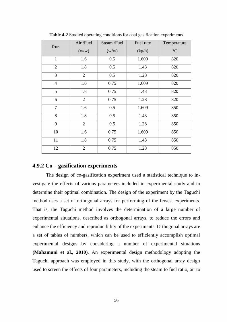
56
Table 4-2 Studied operating conditions for coal gasification experiments
Run Air /Fuel
(w/w)
Steam /Fuel
(w/w)
Fuel rate
(kg/h)
Temperature
°C
1 1.6 0.5 1.609 820
2 1.8 0.5 1.43 820
3 2 0.5 1.28 820
4 1.6 0.75 1.609 820
5 1.8 0.75 1.43 820
6 2 0.75 1.28 820
7 1.6 0.5 1.609 850
8 1.8 0.5 1.43 850
9 2 0.5 1.28 850
10 1.6 0.75 1.609 850
11 1.8 0.75 1.43 850
12 2 0.75 1.28 850
4.9.2 Co – gasification experiments
The design of co-gasification experiment used a statistical technique to in-
vestigate the effects of various parameters included in experimental study and to
determine their optimal combination. The design of the experiment by the Taguchi
method uses a set of orthogonal arrays for performing of the fewest experiments.
That is, the Taguchi method involves the determination of a large number of
experimental situations, described as orthogonal arrays, to reduce the errors and
enhance the efficiency and reproducibility of the experiments. Orthogonal arrays are
a set of tables of numbers, which can be used to efficiently accomplish optimal
experimental designs by considering a number of experimental situations
(Mahamuni et al., 2010). An experimental design methodology adopting the
Taguchi approach was employed in this study, with the orthogonal array design
used to screen the effects of four parameters, including the steam to fuel ratio, air to

57
fuel ratio, percent of biomass used and reaction temperature, on the production of
biogas.
Table4-3 Design experiments, with four parameters at three-levels, for the production of
biogas.
parameter levels
1 2 3
A Steam to Fuel (S/F) ratio 0.25 0.5 0.75
B Air to Fuel (A/F) ratio 2.1 2.3 2.5
C Biomass to Coal (B/C) ratio 0.05 0.11 0.25
D Temperature, °C 800 820 850
Table 4-4 Orthogonal array used to design experiments with four parameters at three-
levels.
Experiment
NO.
Parameters and their levels
S/F ratio A/F ratio B/C ratio Temperature
1 1 1 1 1
2 1 2 2 2
3 1 3 3 3
4 2 1 2 3
5 2 2 3 1
6 2 3 1 2
7 3 1 3 2
8 3 2 1 3
9 3 3 2 1
Table 4-5 Experiments for the parameters and levels shown in Table 4-3.
Experiment
NO.
Parameters and their levels
S/F ratio A/F ratio B/C ratio Temperature,
°C
1 0.25 2.1 0.05 800
2 0.25 2.3 0.11 820
3 0.25 2.5 0.25 850
4 0.5 2.1 0.11 850

58
5 0.5 2.3 0.25 800
6 0.5 2.5 0.05 820
7 0.75 2.1 0.25 820
8 0.75 2.3 0.05 850
9 0.75 2.5 0.11 800
4.10 Procedure of gasification experiments:
A. Before each experiment
1. The bed was ensured to be free of any solids from the previous run.
2. The screw feeder and hopper must be free of contaminants. The screw
feeder was turned on with no coal in the hopper to allow any contaminants
to be completely removed.
3. The furnace walls must be in place before switching on the heating
elements.
4. All valves were ensured to be correctly opened / closed as appropriate.
B. Requirements of experiments
1. Fuel was prepared beforehand: sieving, drying, and weighing.
2. Inert material (sand) required as fluidising medium.
C. The experimental procedure
The experimental procedure for running the gasification unit includes the
following steps:
1. Air-dried fuel was inserted into the hopper, and pre-determined amount of
bed material added into the reactor through the top, then top of reactor sealed
with flange system.
2. Nitrogen was fed to the fuel hopper.
3. Screw feeder cooling water was turned on.
4. Air flow was set at 70 l/min to start fluidization of the bed material.

59
5. Air preheater and heating elements were turned on to pre-heat the furnace
and bed to the desired temperatures.
6. The contactor, control element, and power point were turned on from the
fluid-bed-furnace control panel.
7. The computer connected to the control panel was turned on and software
PicoLog started to record the furnace, bed, and freeboard temperatures and
pressure drop inside the gasifier. During the reaction the temperature can be
changed to the required value using the control panel by either choosing a set
point temperature for Tfurnace or by increasing or decreasing the air heater
temperature or steam flow rate as appropriate.
8. Steam needed for the run to use with air as gasification agent, the water
valve was turned on at a flow rate to obtain the ratio of steam required. The
water was mixed with air out from the heater, thus water can be evaporated
due to the high air temperature.
9. Once the temperature has reached desired level, the fuel feeding was started
at the desired rate by turning on the screw feeder, and the speed of fuel
feeder was dependent on the mass of fuel needed for each experiment.
10. The gas flow rate was decreased to 35 l/min when the temperature of the bed
reaches 400 °C, to control the bed at minimum fluidization case.
11. After bed temperature be 450 °C fuel was fed to the gasifier, so gasification
process will start and the temperature of the bed started to increase gradually
until reaches the desired reaction temperature, then steam starting to pass
through the gasifier.
12. When the steady state has been reached, gas samples were drawn four times
after each hour from the reactor by the gas sampling port.
D. Shut down Procedure
1. Once the experiment has completed, heating elements and air preheater were
switched off, and then the air completely (slump the bed) switched off to
reduce the temperature to ambient conditions over time.

60
2. Once cool, cooling water for feeder was turned off, also the nitrogen flow to
the hopper was turned off and the contents of bed were removed by
discharging the solids at the bottom.
4.11 Composition Measurement
4.11.1 Scanning Electron Microscope
The raw algae before and after leaching, agglomerate from coal gasification,
agglomerate from algae gasification, and bed material from algae gasification were
examined by a scanning electron microscope (Figure 4-10) located at the Adelaide
Microscopy/Medical School, SA, Australia.
For this process a small sample was inserted inside the microscope and two
detectors were used; SE detector (Secondary Electron Detector) and BSE
(Backscattered Electron Detector). SE is used to investigate the structural nature of
the material and BSE for the variation in elemental composition. The BSE detector
works based on elemental ―hardness‖, the harder the element is, the higher the level
of electron reflection will be resulting in a lighter shade in the image obtained.
Figures, peeks, and compositions of the analyzed samples under SE and BSE
detectors are shown in Appendix E.
Figure 4-9 Photographic picture of the Scanning Electron Microscope

61
4.11.2 Gas Chromatography
Agilent 3000 Micro Gas Chromatograph was used to analyse gas samples with
thermal-conductivity detector (TCD). The major advantage of GC over other separation
techniques is the high selective ability to separate volatile components from the gas
mixture. The oven temperature of the gas chromatography is programmed at inlet
temperature of 90 °C and raised to 108 °C. Injection time was 25 seconds and rotation
time was 2 minutes. The carrier gases used for chromatographic analysis were pure
helium and argon, Cerity NDS for Chemical QA/QC software was used to analyze the
samples and produce molar concentrations from the peaks obtained.
Figure 4-10 Gas Chromatography

62
Chapter five
Results and Discussions
5.1 Minimum fluidization velocity
The minimum fluidization velocity was obtained by measuring the pressure
drop across the bed at different superficial velocities and plotting the results. The
results are listed in Table B-1.
Figure (5-1) shows the values of air superficial velocity with changing the
pressure drop. The value of minimum fluidization velocity is found to be equal to
0.09 m/s at 25 oC, and 0.135 m/s at 400
oC for the particle diameter of 0.6-0.71 mm.
The value of minimum fluidization velocity is corrected at 400 oC as shown in
Appendix B.2.
Figure 5-1 Relation between bed pressure drop and air superficial velocity at 25
oC
5.2 Gasification of coal
The fraction of carbon converted during gasification and the amount of each
major component found in the producer gas allow the conclusion of how
gasification reactions are behaving in the reactor. Table 5-1 lists the gasification
reaction.
0
200
400
600
800
1000
1200
1400
0 0.1 0.2 0.3 0.4 0.5
∆P
, pa
U◦, m/s

63
Table 5-1 Gasification reactions (Heiskanen, 2011; Ciferno, and Marano, 2002)
Exothermic Reactions Reaction number
(1)
(2)
(3)
(4)
(5)
Endothermic Reactions
(6)
(7)
(8)
5.2.1 Effect of temperature
Reaction temperature is one of the most important operating parameters
affecting the performance of coal gasification.
The temperature of the bed increases rapidly after fuel feeding. This increase is
happening from the homogenous mixing of the bed material (which acts as a heat
carrier medium) with the fuel inside the gasifier, and also due to the heat produced
from a limited amount of combustion present in the gasifier. In the present study the
gasifier operated with different temperature values (820 and 850) oC to study the
mechanism of gasification reactions at these temperatures.
Figure 5-2 shows the variation of produced molar hydrogen composition with
time at coal feeding rate of 1.28 kg/h, S/F=0.5, and at bed temperature of 850 oC
and 820 oC, respectively. Running the gasifier with a feed flow rate of 1.28 kg/h and
a S/F ratio of 0.5 results in a maximum molar composition of hydrogen of 0.1374 at
820 oC and with the same coal rate, and S/F ratio, the maximum molar composition
of hydrogen produced is 0.147 at 850 oC.
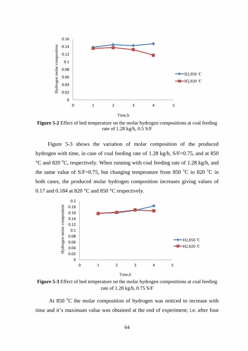
64
Figure 5-2 Effect of bed temperature on the molar hydrogen compositions at coal feeding
rate of 1.28 kg/h, 0.5 S/F
Figure 5-3 shows the variation of molar composition of the produced
hydrogen with time, in case of coal feeding rate of 1.28 kg/h, S/F=0.75, and at 850
°C and 820 oC, respectively. When running with coal feeding rate of 1.28 kg/h, and
the same value of S/F=0.75, but changing temperature from 850 oC to 820
oC in
both cases, the produced molar hydrogen composition increases giving values of
0.17 and 0.184 at 820 °C and 850 °C respectively.
Figure 5-3 Effect of bed temperature on the molar hydrogen compositions at coal feeding
rate of 1.28 kg/h, 0.75 S/F
At 850 oC the molar composition of hydrogen was noticed to increase with
time and it‘s maximum value was obtained at the end of experiment; i.e. after four
0
0.02
0.04
0.06
0.08
0.1
0.12
0.14
0.16
0 1 2 3 4 5
Hyd
rogen
mo
lar
com
po
siti
on
Time,h
H2,850 C
H2,820 C
0
0.02
0.04
0.06
0.08
0.1
0.12
0.14
0.16
0.18
0.2
0 1 2 3 4 5
Hyd
rogen
mo
lar
com
po
siti
on
Time,h
H2,850 C
H2,820 C

65
hours reaction time. This happens due to increase the heat inside the gasifier
resulting in consumption of the rest of steam and unconverted carbon by reactions 7
and 8 and that explains the trends of hydrogen curves in Figure 5-2 and 5-3. While
at 820 °C the molar composition of the produced hydrogen starting to increase and
then decreased at reaction time of 3 hours and continue to slightly decrease until the
end of experiment, and the molar composition of CH4 increases with time and that
is happening due to consuming of the excess hydrogen in the gasifier by reaction 4
and 8 producing more CH4.
Figure 5-4 shows the molar composition of CO2, CO, and CH4 produced when
running the gasifier with 1.28 kg/h, 0.5 S/F at 850 oC and 820
oC, respectively.
Figure 5-4 Effect of bed temperature on the molar compositions of the produced gas
component at run of 1.28 kg/h coal feed rate
The same coal feed rate of 1.28 kg/h with increasing the S/F to 0.75 is
performed with two different temperatures 850 °C and 820 °C, the molar
compositions of CO2, CO, and CH4 produced in this case are shown in Figure 5-5.
0
0.02
0.04
0.06
0.08
0.1
0.12
0.14
0.16
0.18
CO2 CO CH4
Mo
lar
gas
co
mp
osi
tio
n
820,0.5 S/F
850,0.5 S/F
producer gas components

66
Figure 5-5 Effect of bed temperature on the molar compositions of the produced gas
component at run of 1.28 kg/h coal feed rate
The produced CO2 is found to decrease with increasing temperature from
average molar composition of 0.155138 at 820 °C, 0.5 S/F ratio to 0.13154 at 850
oC, 0.5 S/F ratio and from 0.156027 at 820 °C, 0.75 S/F ratio to 0.144742 at 850
oC,
0.75 S/F ratio, while the produced CO and CH4 is increasing with temperature. The
average molar compositions for CO are 0.090319 and 0.111742 at 820 °C, 0.5 S/F
ratio and 850 oC, 0.5 S/F ratio respectively (Figure 5-4). When increasing the S/F
ratio to 0.75 the average molar composition of CO increases from 0.08331 to
0.109389 at 820 and 850 oC respectively. CH4 average molar compositions are
increasing from 0.008779 at 820 °C, 0.5 S/F ratio to 0.010384 at 850 oC, 0.5 S/F
ratio and at 0.75 S/F ratio the average molar compositions of CH4 is increased from
0.011679 to 0.01219 at 820 °C and 850 oC respectively (Figure 5-5).
The experimental results reveal that the composition of CO2 decreases with
temperature in case of 1.28 kg/h coal feed rate while the concentrations of CO and
CH4 increase. This occurs because of the increase in heat within the reactor driving
the reaction to the right producing more CO. Also, reaction 1 is favoured over
reaction 3 so at higher temperatures due to the lower heat of reaction. This will
result in an increase in the carbon converted to CO and decrease in the carbon
converted to CO2. An increase in the hydrogen produced in reaction 5 will increase
0
0.02
0.04
0.06
0.08
0.1
0.12
0.14
0.16
0.18
CO2 CO CH4
Mo
lar
gas
co
mp
osi
tio
n
Producer gas components
820,0.75 S/F
850,0.75 S/F

67
the conversion of carbon to CH4 by reaction 4. In addition, the excess CO present in
the system will drive reaction 8 to the left producing more CH4. The tendency of
CO2 decrease and CO and CH4 increase with temperature increase has been found
by Gonzáleza et al., (2008).
Figure 5-6 shows the variation of produced molar hydrogen composition
with time at coal feeding rate of 1.43 kg/h, S/F=0.5, and at 850 °C and 820 °C,
respectively. The molar hydrogen compositions in the runs performed with 1.43
kg/h mass rate of coal and 0.5 S/F, at both 820 oC and 850
oC, are 0.1343 and
0.1582 respectively.
Figure 5-6 Effect of bed temperature on the molar hydrogen compositions at coal feeding
rate of 1.43 kg/h, 0.5 S/F
Figure 5-7 shows the variation of produced molar hydrogen composition
with time at coal feeding rate of 1.43 kg/h, S/F=0.75, and at 820 °C and 850 oC, the
compositions of hydrogen are 0.15107 and 0.1989 at 820 oC and 850
oC
respectively. The molar hydrogen composition increased with increasing
temperature at the same ratio of steam to fuel and the same mass of coal used with
both runs.
0
0.02
0.04
0.06
0.08
0.1
0.12
0.14
0.16
0.18
0 1 2 3 4 5
Hyd
rogen
mo
ar c
om
po
siti
on
Time,h
H2,850 C
H2,820 C

68
Figure 5-7 Effect of bed temperature on the molar hydrogen compositions at coal feeding
rate of 1.43 kg/h, 0.75 S/F
Figure 5-8 shows the molar composition of CO2, CO, and CH4 produced
when running the gasifier with 1.43 kg/h, 0.5 S/F at 850 oC and 820 °C,
respectively.
Figure 5-8 Effect of bed temperature on the molar compositions of the produced gas
component at run of 1.43 kg/h coal feed rate
The same coal feed rate of 1.43 kg/h with increasing the S/F to 0.75 is
performed with two different temperatures 850 oC and 820 °C. The molar
compositions of CO2, CO, and CH4 produced in this case are shown in Figure 5-9.
The molar compositions of CO2, CO, and CH4 increasing with temperature increase.
0
0.05
0.1
0.15
0.2
0.25
0 1 2 3 4 5
Hyd
rogen
co
mp
ost
ion
Time,h
H2,850 C
H2,820 C
0
0.02
0.04
0.06
0.08
0.1
0.12
0.14
0.16
CO2 CO CH4
Mo
lar
gas
co
mp
osi
tio
n
Producer gas component
820,0.5 S/F
850,0.5 S/F

69
Figure 5-9 Effect of bed temperature on the molar compositions of the produced gas
component at run of 1.43 kg/h coal feed rate
The average molar compositions of CO2, CO, and CH4 increasing with
temperature increase. At 0.5 S/F ratio the CO2 average molar compositions obtained
are 0.13729, and 0.139534 at 820 and 850 oC respectively, while at 0.75 S/F ratio
the average molar compositions of CO2 are 0.161112 and 0.19764 at 820 and 850
oC respectively. The average CO molar compositions at 0.5 S/F ratio are 0.098326
at 820 and 0.111467 at 850 oC, and their average compositions obtained at 0.75 S/F
ratio are 0.086391 and 0.094026 at 820 and 850 oC respectively. CH4 average molar
compositions are increasing from 0.011086 at 820 °C, 0.5 S/F ratio to 0.012946 at
850 oC, 0.5 S/F ratio and at 0.75 S/F ratio the average molar compositions of CH4
increased from 0.013067 to 0.019034 at 820 and 850 oC respectively (Figure 5-8
and 5-9).
Figure 5-10 shows the variation of produced molar hydrogen composition
with time at coal feeding rate of 1.6 kg/h, S/F=0.5, at 850 oC and 820 °C. From the
run completed with a coal mass flow rate of 1.6 kg/h, S/F ratio of 0.5, and
temperature of 820 °C, the maximum molar hydrogen composition in the produced
gas obtained is 0.1305. At the same mass rate of coal and steam to fuel ratio, but at
850 oC, the composition of maximum hydrogen produced obtained is 0.1718. The
molar composition of the produced hydrogen increases with increasing temperature.
0
0.05
0.1
0.15
0.2
0.25
CO2 CO CH4
Mo
lar
gas
co
mp
osi
tio
n
Producer gas components
820,0.75 S/F
850,0.75 S/F

70
Figure 5-10 Effect of bed temperature on the molar hydrogen compositions at coal feeding
rate of 1.6 kg/h, 0.5 S/F
Figure 5-11 shows the variation of produced molar hydrogen composition
with time at coal feeding rate of 1.6 kg/h, S/F=0.75, and at 850 oC and 820 °C,
respectively, the maximum molar hydrogen compositions in this case are 0.1499
and 0.20539 respectively. It can be noticed that increasing temperature cause an
increase in the molar composition of hydrogen produced.
Figure 5-11 Effect of bed temperature on the molar hydrogen compositions at coal feeding
rate of 1.6 kg/h, 0.75 S/F
From the above 12 runs, the average hydrogen molar composition increases
with increasing temperature and according to Le Chatelier's principle ―If a
chemical system at equilibrium experiences a change in concentration,
0
0.02
0.04
0.06
0.08
0.1
0.12
0.14
0.16
0.18
0.2
0 1 2 3 4 5
Hyd
rogen
mo
lar
com
po
siti
on
Time,h
H2,850 C
H2,820 C
0
0.05
0.1
0.15
0.2
0.25
0 1 2 3 4 5
Hyd
rogen
mo
lar
com
po
siti
on
Time,h
H2,850 C
H2,820 C

71
temperature, volume, or partial pressure, then the equilibrium shifts to
counteract the imposed change and a new equilibrium is established‖, after
combustion reactions (1, 2, and 3) have been started the heat inside the gasifier will
rise due to the heat from the oxidation reactions. Therefore; the endothermic
reactions (6 and 7), and shift reaction (8) to the right direction will increase to
consume the produced heat inside the gasifier and that explains the increase in the
average molar composition of the produced hydrogen.
This tendency (higher temperatures produce higher H2 concentrations) has been
found by Neogi et al., (1986); Xiao et al., (2006); and Gonzáleza et al., (2008).
Figure 5-12 shows the molar composition of CO2, CO, and CH4 produced
when running the gasifier with 1.6 kg/h, 0.5 S/F at 850 oC and 820 °C.
Figure 5-12 Effect of bed temperature on the molar compositions of the produced gas
component at run of 1.6 kg/h coal feed rate
Figure 5-13 shows the molar composition of CO2, CO, and CH4 produced
when running the gasifier with 1.6 kg/h, 0.75 S/F at 850 oC and 820 °C.
0
0.02
0.04
0.06
0.08
0.1
0.12
0.14
0.16
0.18
0.2
CO2 CO CH4
Mo
lar
gas
co
mp
osi
tio
n
Producer gas components
820,0.5 S/F
850,0.5 S/F

72
Figure 5-13 Effect of bed temperature on the molar compositions of the produced gas
component at run of 1.6 kg/h coal feed rate
The produced CO2 is found to increase with increasing temperature from
average molar composition of 0.159844 at 820 °C, 0.5 S/F ratio to 0.183927 at 850
oC, 0.5 S/F ratio and from 0.179247 at 820 °C, 0.75 S/F ratio to 0.198412 at 850
oC,
0.75 S/F ratio, while the produced CO and CH4 is increasing with temperature. The
average molar compositions for CO are 0.090233 and 0.096971 at 820 °C, 0.5 S/F
ratio and 850 oC, 0.5 S/F ratio respectively, and when increasing the S/F ratio to
0.75 the average molar composition of CO increases from 0.101412 to 0.108606 at
820 °C and 850 oC respectively. CH4 average molar compositions are increasing
from 0.010321 at 820 °C, 0.5 S/F ratio to 0.014638 at 850 oC, 0.5 S/F ratio and at
0.75 S/F ratio the average molar compositions of CH4 increased from 0.012354 to
0.018672 at 820 °C and 850 oC respectively.
When increasing the fuel feed rate from 1.28 kg/h to 1.43 kg/h and then to 1.6
kg/h with the same operating conditions of bed temperature of 820 °C and 850 oC
and at S/F ratios of 0.5 and 0.75 the produced CO2, CO, H2, and CH4 is increased
with increasing temperature. The increase in CO2 molar composition happens due to
burning more coal by reaction 3 which results in more CO2, the produced CO2 will
react with the unconverted carbon producing more CO by reaction 6. The
composition of hydrogen started to increase with time and its maximum molar
0
0.05
0.1
0.15
0.2
0.25
CO2 CO CH4
Mo
lar
gas
co
mp
osi
tio
ns
Producer gas components
820,0.75 S/F
850,0.75 S/F

73
composition is obtained at the second hour then it is slightly decreased at the third
and fourth hour so this trend in hydrogen composition is due to hydrogen reaction
with the excess unconverted carbon producing more methane and that explains the
increase in methane molar compositions.
5.2.2 Effect of steam to fuel ratio
Figure 5-14 shows the molar compositions of the produced gas component at
the first hour when running with 1.43 kg/h coal feed rate and 0 S/F, at 850 oC. The
experimental molar compositions for CO, CO2, H2, and CH4 are 0.154, 0.137,
0.0829, and 0.0111 respectively.
Operating with a feed rate of 1.43 kg/h at a bed temperature of 850 oC and no
steam result in a rapid increase in bed temperature to 1100 °C after two hours, this
might be due to agglomeration of coal. Agglomeration and defluidization are major
inhibitors to the use of fluidized-bed technology; agglomeration is generally caused
when the bed temperature exceeds a critical temperature, which is sometimes
referred to as the ―sintering point‖. Above the sintering point, bed particles enter a
softened or sticky state. This reduces relative movement between particles and
results in particle growth. Under worst-case conditions, the bed ceases to fluidize
effectively or ―defluidizes‖. Controlling agglomeration and defluidization is thus
0
0.02
0.04
0.06
0.08
0.1
0.12
0.14
0.16
0.18
0.4 0.6 0.8 1 1.2
Mo
lar
gas
co
mp
osi
tio
n
Time,h
CO2
H2
CH4
CO
Figure 5-14 Produced gas component distribution at the first hour of 1.43kg/h coal feed rate
and 0 S/F, at 850 oC

74
critical for any commercial fluidized-bed process; agglomeration at temperature
above 850 °C is similar to the result obtained by McCullough and Eyk, (2011).
This agglomerate was analysed using Scanning Electron Microscopy (SEM)
by Secondary Electron Detector (SE) and Backscattered Electron Detector (BSE) to
know the compositions of materials in this agglomerate. Photographic pictures were
taken under SE detector and the compositions of the resulted peeks were generated
Figure E-1and E-2.
Backscattered Electron Detector (BSE) was used to get information on the Z
contrast of the sample (Z = atomic number), where regions that contain atoms with
high Z will be viewed as bright regions, and conversely atoms with low Z as dark
regions Figure E-3 and E-4.
Agglomeration during gasification of coal occurs due to defluidization, the bed
temperature excess the ―high- temperature defluidization limit‖ which means less
value of superficial velocity to avoid defluidization case for a known bed
temperature. Defluidization will lead to particle growth and will be in a stationary
case in the annulus, while a channel in the spout region will form and the air could
pass freely through. ―Sintering point‖ will decrease by increasing the superficial
velocity of the gas which increase the movement of the bed particles, or by
decreasing the bed temperature.
Figure 5-15 Photographic picture of the agglomerate collected after the run

75
In the present study decreasing bed temperature was suggested by using (air-
steam) gas mixture as gasification agent. Injection of steam through the gasifier
with (0.5 and 0.75 S/F) will decrease the bed temperature due to the energy
consuming for water evaporation.
Figure 5-16 shows the variation of hydrogen molar compositions in the
produced gas for the coal mass rate of 1.28 kg/h, 820 °C, at 0.75 and 0.5 S/F.
Increasing the S/F ratio causes the molar hydrogen composition to increase.
Figure 5-16 Effect of S/F ratio on the molar hydrogen compositions at coal mass rate of
1.28 kg/h, 820 °C
Figure 5-17 shows the variation of hydrogen molar compositions in the
produced gas for the coal mass rate of 1.28 kg/h, 850 oC, at 0.75 and 0.5 S/F
respectively. Increasing the S/F ratio causes the molar hydrogen composition to
increase.
0
0.02
0.04
0.06
0.08
0.1
0.12
0.14
0.16
0.18
0 1 2 3 4 5
Hyd
rogen
mo
lar
com
po
siti
on
Time,h
H2,0.75 S/F
H2,0.5 S/F

76
Figure 5-17 Effect of S/F ratio on the molar hydrogen compositions at coal mass rate of
1.28 kg/h, 850 oC
Figure 5-18 shows the molar composition of CO2, CO, and CH4 in the
produced gas when running the gasifier with 1.28kg/h coal feed rate, 820 °C and
850 oC at 0.5 and 0.75 S/F respectively. At the same feed rate and temperature the
molar compositions of CO2 and CH4 increase with increasing the S/F ratio. When
operating the gasifier with coal feed rate of 1.28 kg/h, 820 °C, and S/F of 0.5, the
average molar compositions for CO2, CO, and CH4 are 0.155138, 0.090319, and
0.010384 respectively, while increasing the S/F to 0.75 with the same bed
temperature and coal feed rate the average molar compositions of CO2, CO, and
CH4 are 0.156027, 0.08331, and 0.011679 respectively. Running with 850 C and 0.5
S/F, the average molar compositions of CO2, CO, and CH4 produced are 0.13154,
0.111742, and 0.008779 respectively, increasing the S/F ratio to 0.75 at bed
temperature of 850 oC, the average molar compositions of CO2, CO, and CH4
obtained are 0.144742, 0.109389, and 0.01219 respectively.
0
0.02
0.04
0.06
0.08
0.1
0.12
0.14
0.16
0.18
0.2
0 1 2 3 4 5
Hyd
rogen
mo
lar
com
po
siti
on
Time,h
H2,0.75 S/F
H2,0.5 S/F

77
Figure 5-18 Effect of S/F ratio on the molar compositions of CO2, CO, and CH4 at coal
mass rate of 1.28 kg/h
Figure 5-19 shows the hydrogen molar compositions in the produced gas for
the coal mass rate of 1.43 kg/h, 820 °C, at 0.75 and 0.5 S/F respectively. The molar
composition of hydrogen produced increases with increasing the ratio of steam to
fuel.
Figure 5-19 Effect of S/F ratio on the molar compositions of hydrogen at coal mass rate of
1.43 kg/h and 820 °C.
Figure 5-20 shows the molar compositions of hydrogen in the produced gas
from the run with coal mass rate of 1.43 kg/h, 850 oC, at 0.75 and 0.5 S/F
respectively. The composition of hydrogen in the produced gas was found to
increase with increasing steam to fuel ratio from 0.5 to 0.75 at 820 °C and 850 oC.
0
0.02
0.04
0.06
0.08
0.1
0.12
0.14
0.16
0.18
Mo
lar
gas
co
mp
osi
tio
n
Producer gas components
820 C
850 C
0
0.02
0.04
0.06
0.08
0.1
0.12
0.14
0.16
0 1 2 3 4 5
Hyd
rogen
mo
ar c
om
po
siti
on
Time,h
H2,0.75 S/F
H2,0.5 S/F
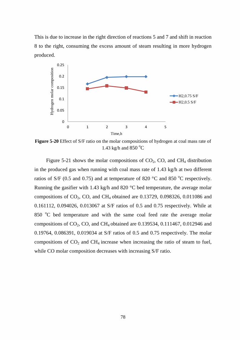
78
This is due to increase in the right direction of reactions 5 and 7 and shift in reaction
8 to the right, consuming the excess amount of steam resulting in more hydrogen
produced.
Figure 5-20 Effect of S/F ratio on the molar compositions of hydrogen at coal mass rate of
1.43 kg/h and 850 oC
Figure 5-21 shows the molar compositions of CO2, CO, and CH4 distribution
in the produced gas when running with coal mass rate of 1.43 kg/h at two different
ratios of S/F (0.5 and 0.75) and at temperature of 820 °C and 850 oC respectively.
Running the gasifier with 1.43 kg/h and 820 °C bed temperature, the average molar
compositions of CO2, CO, and CH4 obtained are 0.13729, 0.098326, 0.011086 and
0.161112, 0.094026, 0.013067 at S/F ratios of 0.5 and 0.75 respectively. While at
850 oC bed temperature and with the same coal feed rate the average molar
compositions of CO2, CO, and CH4 obtained are 0.139534, 0.111467, 0.012946 and
0.19764, 0.086391, 0.019034 at S/F ratios of 0.5 and 0.75 respectively. The molar
compositions of CO2 and CH4 increase when increasing the ratio of steam to fuel,
while CO molar composition decreases with increasing S/F ratio.
0
0.05
0.1
0.15
0.2
0.25
0 1 2 3 4 5
Hyd
rogen
mo
lar
com
po
siti
on
Time,h
H2,0.75 S/F
H2,0.5 S/F
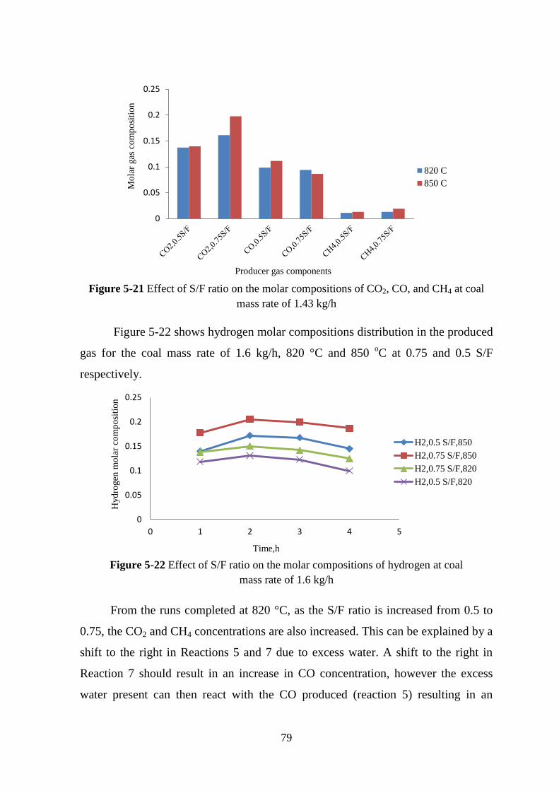
79
Figure 5-21 Effect of S/F ratio on the molar compositions of CO2, CO, and CH4 at coal
mass rate of 1.43 kg/h
Figure 5-22 shows hydrogen molar compositions distribution in the produced
gas for the coal mass rate of 1.6 kg/h, 820 °C and 850 oC at 0.75 and 0.5 S/F
respectively.
Figure 5-22 Effect of S/F ratio on the molar compositions of hydrogen at coal
mass rate of 1.6 kg/h
From the runs completed at 820 °C, as the S/F ratio is increased from 0.5 to
0.75, the CO2 and CH4 concentrations are also increased. This can be explained by a
shift to the right in Reactions 5 and 7 due to excess water. A shift to the right in
Reaction 7 should result in an increase in CO concentration, however the excess
water present can then react with the CO produced (reaction 5) resulting in an
0
0.05
0.1
0.15
0.2
0.25
Mo
lar
gas
co
mp
osi
tio
n
Producer gas components
820 C
850 C
0
0.05
0.1
0.15
0.2
0.25
0 1 2 3 4 5
Hyd
rogen
mo
lar
com
po
siti
on
Time,h
H2,0.5 S/F,850
H2,0.75 S/F,850
H2,0.75 S/F,820
H2,0.5 S/F,820

80
increase in CO2 and H2 production. The extra hydrogen produced can also interact
with CO to produce CH4 (Reaction 8) which explains the increase in CH4.
If the temperature is increased to 850 °C and with both 0.5 and 0.75 S/F and
according to Le Chatelier's principle, endothermic reactions will increase in activity
and exothermic decrease. A higher operating temperature would result in an
increased production of CO by Reactions 6 and 7 which are endothermic. The
excess H2 and CO present is enough to force an increase in production of CH4 by
reaction 4 and 8.
Figure 5-23 shows the molar compositions of CO2, CO, and CH4 distribution
in the produced gas when running with coal mass rate of 1.6 kg/h at two different
ratios of S/F (0.5 and 0.75) and at temperature of 820 °C and 850 oC respectively.
Operating with 1.6 kg/h and 820 °C bed temperature, the average molar
compositions of CO2, CO, and CH4 obtained are 0.159844, 0.090233, 0.010321 and
0.179247, 0.101412, 0.012354 at S/F ratios of 0.5 and 0.75 respectively. While at
850 oC bed temperature and with the same coal feed rate the average molar
compositions of CO2, CO, and CH4 obtained are 0.183927, 0.096971, 0.014638 and
0.198412, 0.108606, 0.018672 at S/F ratios of 0.5 and 0.75 respectively.
Figure 5-23 Effect of S/F ratio on the molar compositions of CO2, CO, and CH4 at coal
mass rate of 1.6 kg/h
0
0.05
0.1
0.15
0.2
0.25
Mo
lar
gas
co
mp
osi
tio
n
Producer gas composition
820 C
850 C

81
5.2.3 Effect of air to fuel ratio
The air to fuel ratio is based on a dry air flow rate and the coal on a dry mass
flow basis. Three different air to fuel ratios were compared (1.6, 1.8 and 2) at two
different temperatures (820 °C and 850 °C) and two different steam to fuel ratios
(0.5 and 0.75). These were achieved by altering the coal mass flow rate with a
constant air flow rate of 35 l/min.
Figure 5-24 shows the molar compositions of hydrogen in the produced gas
when running the gasifier with coal mass rate of (1.28, 1.43, and 1.6 kg/h)
respectively with S/F of 0.5 and temperature of 820 °C. The concentration of
hydrogen in the produced gas is increased with increasing air to fuel ratio when
running with 820 °C. The average hydrogen compositions were 0.1176, 0.1273, and
0.1307 at 1.6, 1.8, and 2 A/F respectively with a S/F ratio of 0.5.
Figure 5-24 Effect of A/F ratio on the molar compositions of hydrogen at S/F of 0.5 and
820 °C.
Figure 5-25 shows the molar compositions of hydrogen in the produced gas
when running with coal mass rate of (1.28, 1.43, and 1.6 kg/h) respectively at S/F of
0.75 and at 820 °C. When running at the same temperature with 0.75 S/F the
hydrogen compositions were found to be 0.1385, 0.146, and 0.1641 at A/F ratios of
1.6, 1.8, and 2 respectively. That increase in hydrogen produced at 820 °C is due to
increase oxygen (A/F) that will shift reaction 5 and 8 to the right direction and more
hydrogen.
0
0.02
0.04
0.06
0.08
0.1
0.12
0.14
0.16
0 1 2 3 4 5
Hyd
rogen
mo
lar
com
po
siti
on
Time,h
H2,1.6 kg/h
H2,1.43 kg/h
H2,1.28 kg/h

82
Figure 5-25 Effect of A/F ratio on the molar compositions of hydrogen at S/F of 0.75 and
820 °C.
Figure 5-26 shows the molar compositions of hydrogen in the produced gas
when running the gasifier with S/F of 0.5 and at 850 oC at A/F ratios of 1.6, 1.8, and
2 respectively. The average hydrogen compositions decrease with increasing air to
fuel ratio and their values are (0.1559, 0.1459, and 0.143531 at A/F ratios
respectively of 1.6, 1.8, and 2).
Figure 5-26 Effect of A/F ratio on the molar compositions of hydrogen at S/F of 0.5 and
850 oC
Figure 5-27 shows the molar compositions of hydrogen in the produced gas
when running the gasifier with S/F of 0.75 and at 850 oC at A/F ratios of 1.6, 1.8,
and 2 respectively. At this case the average molar compositions of hydrogen are
0.1924, 0.1898, and 0.167903 at 1.6, 1.8, and 2 respectively.
0
0.02
0.04
0.06
0.08
0.1
0.12
0.14
0.16
0.18
0 1 2 3 4 5
Hyd
dro
gen
mo
lar
com
po
siti
on
Time,h
H2,1.6 kg/h
H2,1.43 kg/h
H2,1.28 kg/h
0
0.02
0.04
0.06
0.08
0.1
0.12
0.14
0.16
0.18
0.2
0 1 2 3 4 5
Hyd
rogen
mo
lar
com
po
sito
n
Time,h
H2,1.6 kg/h
H2,1.43 kg/h
H2,1.28 kg/h

83
Figure 5-27 Effect of A/F ratio on the molar compositions of hydrogen at S/F of 0.75 and
850 oC
Figure 5-28 shows the molar composition of CO2 produced when running the
gasifier with A/F ratios of 1.6, 1.8 , and 2 respectively, 0.5, and 0.75 S/F ratios, and
at 850 oC and 820 °C, respectively.
At 0.75 S/F and 850 oC bed temperature, the average CO2 compositions
obtained are 0.198412, 0.19764, and 0.144742 at A/F ratios of 1.6, 1.8, and 2
respectively, when the bed temperature decreased to 820 °C and with 0.75 S/F ratio
CO2 average compositions are 0.179247, 0.161112, and 0.156027 at A/F ratios of
1.6, 1.8, and 2 respectively. When running with S/F ratio of 0.5 the average molar
compositions of CO2 at 850 oC are 0.183927, 0.139534, and 0.13154 at A/F ratios
of 1.6, 1.8, and 2 respectively, and with the same S/F but with bed temperature of
820 °C the average CO2 compositions obtained are 0.159844, 0.13729, and
0.155138 at A/F ratios of 1.6, 1.8, and 2 respectively.
0
0.05
0.1
0.15
0.2
0.25
0 1 2 3 4 5
Hyd
rogen
mo
lar
com
po
siti
on
Time,h
H2,1.6 kg/h
H2,1.43 kg/h
H2,1.28 kg/h

84
Figure 5-28 Effect of A/F on the molar composition of CO2 at S/F ratios of 0.5, and 0.75
The produced carbon dioxide decreases from an air to fuel ratio change of 1.6
to 1.8 in all cases except case (850 °C, 0.75 S/F). An increase in the oxygen
available to react with carbon (A/F = 1.6 to A/F = 1.8) results in an increase in the
production of CO by reaction 1. Reaction one is more favoured over 3 as it is less
exothermic, which results in a shift to the right in reaction 5 increasing the
production of CO2 and H2. As the oxygen levels are further increased (A/F = 2), the
amount of CO2 produced by reaction 3 increases and the amount of CO converted to
CO2 by reaction 2 increases. This explains the increase in CO2 from an A/F ratio of
1.8 to 2 in case (820 °C, 0.5 S/F). With extra steam present in the system, reaction 7
can reduce the amount of carbon available for reaction 3 resulting in reduced
production of CO2 (case, 820 °C, 0.75, A/F = 1.8 to A/F = 2). The amount of CO2
produced in case three (850 °C, 0.5) can be explained in the same way as case (820
°C, 0.5) with a much higher CO2 value resulting.
Figure 5-29 shows the molar composition of CO produced when operating
with A/F ratios of 1.6, 1.8 , and 2 respectively, S/F ratios of 0.5, and 0.75 at 850 oC
and 820 °C respectively.
When running with A/F ratios of 1.6, 1.8, and 2 the average molar CO
compositions obtained are 0.108606, 0.08639, and 0.1093 respectively at S/F ratio
of 0.75 and 850 oC, and with the same A/F ratios and the same temperature and 0.5
S/F the average molar CO compositions obtained are 0.096971, 0.111467, and
0.111742 respectively. In the case of running with 820 °C and at S/F ratio of 0.75
0
0.05
0.1
0.15
0.2
0.25
1.6 A/F 1.8 A/F 2 A/F
Mo
lar
gas
co
mp
osi
tio
n
Air to Fuel ratio
CO2,850,0.75S/F
CO2,850,0.5S/F
CO2,820,0.75S/F
CO2,820,0.5S/F

85
the average compositions of CO are 0.101412, 0.094026, and 0.08331 at A/F ratios
of 1.6, 1.8, and 2 respectively, and at 820 °C, 0.5 S/F the average CO compositions
are 0.090233, 0.098326, and 0.090319 at A/F ratios of 1.6, 1.8, and 2 respectively.
Figure 5-29 Effect of A/F on the molar composition of CO at S/F ratios of 0.5 and 0.75
Figure 5-30 shows the molar composition of CH4 produced when operating
with A/F ratios of 1.6, 1.8 , and 2 respectively, S/F ratios of 0.5, and 0.75 at 850 oC
and 820 °C respectively. At 0.75 S/F and 850 oC bed temperature, the average CH4
compositions obtained are 0.018672, 0.019034, and 0.01219 at A/F ratios of 1.6,
1.8, and 2 respectively, when the bed temperature decreased to 820 °C and with
0.75 S/F ratio the average CH4 compositions are 0.012354, 0.013067, and 0.011679
at A/F ratios of 1.6, 1.8, and 2 respectively. When running with S/F ratio of 0.5 the
average molar compositions of CH4 at 850 oC are 0.014638, 0.012946, and
0.008779 at A/F ratios of 1.6, 1.8, and 2 respectively, and with the same S/F but
with bed temperature of 820 °C the average CH4 compositions obtained are
0.010321, 0.011086, and 0.010384 at A/F ratios of 1.6, 1.8, and 2 respectively.
0
0.02
0.04
0.06
0.08
0.1
0.12
1.6 A/F 1.8 A/F 2 A/F
Mo
lar
gas
co
mp
osi
tio
n
Air to Fuel ratio
CO,850,0.75S/F
CO,850,0.5S/F
CO,820,0.75S/F
CO,820,0.5S/F

86
Figure 5-30 Effect of A/F on the molar composition of CH4 at S/F ratios of 0.5 and 0.75
At increased temperatures (850 °C) the opposite trend occurs. The less
exothermic reactions are more favoured which results in more CO produced
(Reaction 1) as the oxygen concentration increases, this reduces the amount of
hydrogen produced by Reaction 7 and as the availability of oxygen is further
increased the carbon dioxide produced by reaction 3 increases which will shift
reaction 5 to the left further decreasing hydrogen concentrations and increasing
carbon monoxide. The methane levels are dependent mainly on hydrogen levels in
the reactor (reactions 4 and 8).
5.2.4 Carbon conversion
The carbon conversion, defined as the degree to which the carbon in the fuel
has been converted into gaseous products, is an important parameter in deciding the
performance of a gasifier (Abdul Salam, 2006). Carbon conversion calculations
were completed based on the assumption that all nitrogen feed into the gasifier left
in the gasifier in the producer gas. Using the assumptions of an atmospheric
nitrogen concentration of 78% (molar percent), atmospheric pressure (101325 pa)
and a temperature at the flow rate meter of 293.15 °C and a slightly altered version
of the ideal gas law, equation (5.1), the flow rate of Nitrogen through the gasifier,
and the total flow rate of the producer gas can be calculated from equation (5.2).
( ) ( )
(5.1)
0
0.002
0.004
0.006
0.008
0.01
0.012
0.014
0.016
0.018
0.02
1.6 A/F 1.8 A/F 2 A/F
Mo
lar
gas
co
mp
osi
tio
n
Air to Fuel ratio
CH4,850,0.75S/F
CH4,850,0.5S/F
CH4,820,0.75S/F
CH4,820,0.5S/F
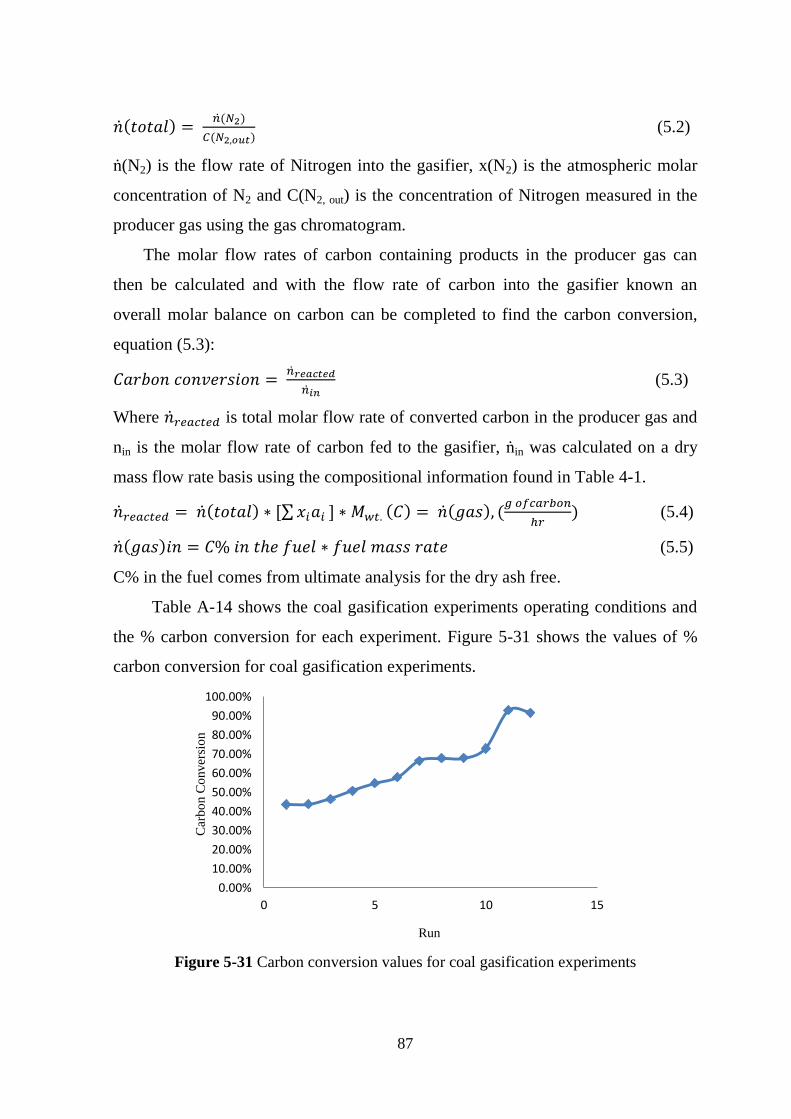
87
( ) ( )
( ) (5.2)
ṅ(N2) is the flow rate of Nitrogen into the gasifier, x(N2) is the atmospheric molar
concentration of N2 and C(N2, out) is the concentration of Nitrogen measured in the
producer gas using the gas chromatogram.
The molar flow rates of carbon containing products in the producer gas can
then be calculated and with the flow rate of carbon into the gasifier known an
overall molar balance on carbon can be completed to find the carbon conversion,
equation (5.3):
(5.3)
Where is total molar flow rate of converted carbon in the producer gas and
nin is the molar flow rate of carbon fed to the gasifier, ṅin was calculated on a dry
mass flow rate basis using the compositional information found in Table 4-1.
( ) ,∑ - ( ) ( ) (
) (5.4)
( ) (5.5)
C% in the fuel comes from ultimate analysis for the dry ash free.
Table A-14 shows the coal gasification experiments operating conditions and
the % carbon conversion for each experiment. Figure 5-31 shows the values of %
carbon conversion for coal gasification experiments.
Figure 5-31 Carbon conversion values for coal gasification experiments
0.00%
10.00%
20.00%
30.00%
40.00%
50.00%
60.00%
70.00%
80.00%
90.00%
100.00%
0 5 10 15
Car
bo
n C
onver
sio
n
Run
88
The maximum value of carbon conversion and maximum H2:CO ratio are
92.9% and 2.197 respectively which are obtained at 1.8 A/F ratio, 0.75 S/F ratio,
and at 850 °C bed temperature this indicates that these operating conditions are the
optimum conditions for coal gasification.
5.3 Algae gasification
Gasification experiments were conducted using algal biomass as a fuel source.
Producer gas compositions were analysed to investigate the mechanism of
gasification reactions present with an alternative source of carbon and how it differs
to that of the mechanisms present in coal gasification. The first problem
encountered with using the algae biomass was in the particle shape and size. The
biomass particles were found to have a lower sphericity than the coal which affected
the flow from the hoppers to the screw feeder. This generated an issue with feeding
halting after approximately half an hour. To avoid this, the particle size diameter
was reduced from between 1 and 3.35 mm to between 1 and 2 mm. The second
major problem faced was with agglomeration of the bed during start up.
Experiments were conducted with a fuel mass rate of 1.43 kg/h, steam to fuel ratio
of 0.5 at a temperature of 850 oC. The fuel was fed into the gasifier after bed
temperature reached 450 °C. With coal this results in a temperature step increase in
the reactor to approximately 840 °C however when this was done with the algae it
was found the temperate reached a value of between 600 °C and 620 °C and
stabilised. Agglomeration happened after feeding the fuel. As the bed material
recovered was stuck together in clumps. Samples of raw algae and agglomerates
from the gasification runs were analysed using SEM (Figures E-5, E-6, E-7, E-8,
and E-9).
SEM images shown in Appendix E.2 show an excess amount of sodium,
aluminium and magnesium chlorides and silica oxide. These could be from the
water used to grow algae (sea water) which is high in salt content. The salt is likely
to have crystallised during the drying process, which is what can be seen in Fig. E-8
and E-8a Silica oxide which is used as a heat carrier medium in the gasification

89
agglomerated in this case and formed clumps with the algae. Agglomeration may be
due to the excess salt present in the algae. High levels of aluminium and magnesium
also had been found which could have something to do with the chemistry
occurring in the reactor.
A sample for the bed material from the run of agglomerated algae was
analysed by SEM secondary electron detector to analyse the structure of this
material (Figure E-9 a, b, c, and d).
From Figure E-9 an excess amount of sodium, aluminium and magnesium
chlorides and silica oxide can be seen in the bed material resulting from algae
gasification. Looking at the chemistry of Al and Cl there is a possibility that the
sodium chloride is interacting with water to form Cl2, H2 and NaOH. The Cl2
produced is then free to react with Al to produce AlCl3 which forms a liquid at
temperatures above 192.4 °C. It is also interesting to see that the reaction required
for the formation of AlCl3 is favoured around 650-750 °C which is close to the
temperature the gasifier reaches before agglomeration occurs.
In industry, elemental chlorine is usually produced by the electrolysis of
sodium chloride dissolved in water. Along with chlorine, this chloralkali process
yields hydrogen gas and sodium hydroxide, according to the following chemical
equation (Galatsis, 1999).
2 NaCl + 2 H2O → Cl2 + H2 + 2 NaOH (9)
Aluminium chloride is manufactured on a large scale by the exothermic reaction of
aluminium metal with chlorine or hydrogen chloride at temperatures between 650 to
750 °C (Greenwood and Earnshaw, 1984).
2 Al + 3 Cl2 → 2 AlCl3 (10)
2 Al + 6 HCl → 2 AlCl3 + 3 H2 (11)
Aluminium chloride is hygroscopic, having a very high affinity for water. It fumes
in moist air and hisses when mixed with liquid water as the Cl- ions are displaced
with H2O molecules in the lattice to form the hexahydrate AlCl3•6H2O (white to
yellowish in colour). The anhydrous phase cannot be regained on heating as HCl is
lost leaving aluminum hydroxide or alumina (aluminum oxide):

90
Al(H2O)6Cl3 → Al(OH)3 + 3 HCl + 3 H2O (12)
On strong heating (~400 °C), the aluminum oxide is formed from the aluminum
hydroxide by:
Al(OH)3 → Al2O3 + 3 H2O (13)
To ensure efficient gasification for the algae, leaching of raw algae is
considered to dissolve the salt contained by this algae. Raw algae was examined by
SEM secondary- electron detector to investigate the structural nature of the material
before and after leaching. It was noticed that sodium chloride content in algae is
decreased due to leaching Figures E-10 and E-11.
From Figure E-11, it can be shown that leaching of raw algae causes the salt
content in raw algae to dissolve and that may prevent agglomeration problem from
happening in the gasification experiments when using leached algae.
5.3.1 Co-gasification (Coal-Algae, gasification)
Co-gasification was completed using 90% coal and 10% algae to study the
mechanism of gasification reactions present for this fuel composition, and to
investigate whether or not agglomeration would occur with a lower flow of biomass
into the gasifier. The gasifier was operated with air and steam to fuel ratios of 2 and
0.5 respectively at a temperature of 820 °C. After beginning fuel feeding the
temperature increases rapidly to 820 °C, gas samples were withdrawn at different
periods (30, 45, 60, 75, and 90 minutes) . The bed temperature continued to rise
steadily until the gasifier had to be shut down to prevent agglomeration.
Figure 5-32 shows the molar compositions of H2, CO2, CO, and CH4 result
from co-gasification experiment with 10% algae + 90% coal, with S/F and A/F
ratios of 0.5 and 2 respectively and at 820 °C. The bed temperature fluctuating at
different values starting from 830, 840, 850, 860, 870, and 880 °C, the increase in
temperature is happening each 15 min, which means there is a problem within the
bed inside the gasifier. The composition of hydrogen in the producer gas was
noticed to decrease with time and with temperature increase and that trend is wrong,

91
according to gasification reactions and while the temperature increase the molar
composition of hydrogen in the produced gas should increase.
Figure 5-32 Producer gas molar compositions from (algae-coal) gasification
Agglomeration doesn‘t occur however high levels of pressure and bed temperature
were reached after 90 minutes. This might have resulted from decreased bed
fluidisation, or it could have been due to interaction of potassium carbonate with
minerals present in the coal at higher loadings. After the gasifier was cooled down,
the bed material was recovered and there were no agglomerates found. The tubes
for passing the producer gas were disconnected and found to be blocked with
grey/black ash.
A sample of the gray material blocking the pipes was taken and the salt
content was tested. The salt level in the blockage was the same in the raw algae
0
0.02
0.04
0.06
0.08
0.1
0.12
0.14
H2 CO2 CO CH4
gas
mo
lar
com
po
siti
on
Producer gas components
830
840
860
870
880
Figure 5-33 Blockages in the outer tubes of the gasifier

92
which means that blockage lead to raw algae. The raw algae may be crushed in the
screw feeder because it is soft and entered the gasifier as fine particles and smaller
diameter than coal particles, and affecting by the air flow coming from the bottom
of the gasifier and because the place of passing the producer gas nearer to the place
of screw feeder more than the bed. The fine particles will pass easily through the
outer tubes with the producer gas and gathered in these tubes with time and that will
cause the inside gasifier temperature to increase with time because the producer gas
will have a difficulty to pass through the out tubes and high pressure will results
inside the gasifier. After 90 minutes the temperature reached to 950 °C and
hydrogen composition in the producer gas was decreased with time.
5.4 Co-gasification (coal-grape seeds gasification)
First experiment was conducted with air to fuel and steam to fuel ratios of 2
and 0.5 respectively, 5 % grape seeds biomass at 820 °C. The fuel started to feed
through the gasifier and the bed temperature started to increase gently, the samples
were taken every 30 minutes after steady state. The hydrogen in the producer gas
was increased at 30 to 60 minutes and the bed temperature was controlled. After the
first hour the bed temperature started to increase rapidly with time and reached to
950 °C and the last gas sample was taken after 75 minutes and then the gasifier was
shut down to prevent agglomeration. The bed material was removed after the
gasifier had been cooled down, some sand particles were agglomerated. All the
outer tubes were checked if any blockages might be happened and all of them were
clean and empty. Therefore, the problem lead to the compositions of biomass
because the coal was tested before with the same operating conditions of this
experiment and succeeded. The air to fuel ratio of 1.8 was tested with 0.5 steam to
fuel ratio at 820 °C, and 5% grape seeds, the temperature was increased further and
faster than the previous case and 20 minutes after steady state the bed temperature
increased to 990 °C and was shut down without taking gas sample.

93
Figure 5-34 shows the molar compositions of H2, CO2, CO, and CH4 result
from coal-grape seeds gasification with air to fuel and steam to fuel ratios of 2 and
0.5 respectively, 5 % grape seeds biomass at 820 °C.
Figure 5-34 Molar compositions of producer gas component result from Co-gasification.
It is concluded that the bed temperature increased rapidly with increasing the
mass of fuel feeding to the gasifier or in other word with increasing the mass of
biomass feeding to the gasifier. Looking at the chemical analysis of the biomass,
(Table C-3) it noticed to contain much amount of potassium oxide which can be
responsible for increasing the bed temperature. After the fuel was fed gasification
reactions will start and the producer gas contains CO2 which can react with
potassium oxide in the grape seeds forming potassium carbonate K2CO3 by the
following reaction:
(14)
Potassium carbonate (K2CO3), formed in the char, can be reacting with silicon
from the bed material leading to the formation of molten potassium silicates. A
possible reaction to describe this process is:
(15)
The sodium analog of reaction (15) has been documented to form a liquid
sodium silicate melt (Eyk, et al., 2009). So that the formation of molten potassium
0
0.02
0.04
0.06
0.08
0.1
0.12
0.14
0.16
20 30 40 50 60 70 80 90
Mo
lar
gas
co
mp
osi
tio
n
Time, min.
CO2
H2
CH4
CO

94
and sodium silicate can be accumulated with time and form a layer on the top of the
bed which prevent the gas to pass easily and also will lead to decrease or stop the
gasification reactions to continue, and that will increase the temperature of the bed
because defluidization will happen. To avoid this problem increasing the ratio of air
to fuel was suggested to prevent or reduce the formation of the molten components
in the bed.
Three ratios of air to fuel (2.1, 2.3, and 2.5) were performed in co-gasification with
three steam to fuel ratios (0.25, 0.5, and 0.75) at different temperatures (800, 820,
and 850 °C) with three different biomass to coal ratios (0.05, 0.11, and 0.25), set of
the completed experiments are shown in Table 4-3. These experiments are done
depending on Taguchi method of experiments design.
5.4.1 Determination of Percentage Contribution of Individual
Variables
The carbon conversion producing biogas in a gasifier by nine set of
gasification experiments (Table 4-3). From the experimental results carbon
conversion has been calculated for each experiment and maximum value of carbon
conversion is obtained at experiment number 8 which has a carbon conversion of
95.59345% which mean to have the best experimental conditions while the lowest
conversion has been obtained at experiment number 5 and it is equal to 63.6665%.
Taguchi method has been applied for the design of an experiment to study the best
experimental conditions.
In Taguchi method, the signal-to-noise (S/N) ratio is used to measure the
quality characteristics deviating from the desired value. The S/N ratios are different
in terms of their characteristics, of which there are generally three types, i.e.
smaller-the-better, larger-the-better and normal-the-better. According to the analysis
for the case of ‗larger-the-better‘, the mean squared deviations (MSD) of each
experiment were evaluated using the following equation:
∑ 0
1
(5.6)

95
Where n is the number of repetitions of each experiment and yi carbon conversion.
Then, the S/N ratio was evaluated using the following equation (Taguchi, 1986):
( ) (5.7)
The S/N ratios for the nine sets of experiments are shown in Table 5-2. The mean
carbon conversion and the mean S/N ratio are 82.72613% and 38.28649%,
respectively. Experiment number 8 gave the highest conversion and had the largest
S/N ratio.
Table 5-2 % Carbon conversion, MSD, and S/N ratios for the nine set of gasification
experiments
Experiment No. % Carbon
conversion MSD S/N
1 73.68429813 0.000184183 37.34749902
2 82.95197591 0.000145327 38.37653471
3 95.21793407 0.000110297 39.57437509
4 81.52657251 0.000150453 38.22598369
5 63.6665338 0.000246705 36.07822412
6 90.51054095 0.000122068 39.13398321
7 86.15732146 0.000134715 38.70584378
8 95.59345163 0.000109432 39.60856286
9 75.22657517 0.000176708 37.5274258
Mean carbon
conversion% =
82.72613374
Mean S/N ratio =
38.28649248
The mean S/N ratio was calculated from the effect of the variables and the
interactions at assigned levels this means the average of all the S/N ratios of a set of
control variables at a given level. For example, in the case of variable A and level 1,
the mean S/N ratio (38.4328029) was calculated using the values (37.34749902,
38.37653471 and 39.57437509) from experiment numbers 1 to 3. In the case of
parameter A and level 2, the mean S/N ratio (37.8127303) was calculated using the
values (38.22598369, 36.07822412 and 39.13398321) from experiment numbers 4

96
to 6, and so on. The calculated values of the mean S/N ratios and the difference
between two levels can be shown in Table 5-3 and 5-4 respectively.
Table 5-3 Mean S/N ratios
Variables Levels
1 2 3
A S/F ratio 38.4328029 37.8127303 38.61394415
B A/F ratio 38.0931088 38.0211072 38.74526137
C B/C ratio 38.6966817 38.04331473 38.119481
D Temperature, °C 36.984383 38.7387872 39.13630721
Table 5-4 Difference between two levels
Parameters Difference
L2-1 L3-1 L3-2
A S/F ratio -0.620072598 0.1811412 0.801213807
B A/F ratio -0.072001596 0.6521525 0.724154136
C B/C ratio -0.653366965 -0.5772007 0.076166263
D Temperature, °C 1.754404248 2.1519242 0.397519982
The contribution for each variable calculated from the maximum difference
of mean S/N ratios between two levels for each variable Table 5-5.
Table 5-5 % Contribution for each variable
Parameters Max. difference Contribution (%)
A S/F ratio 0.801213807 21.34601516
B A/F ratio 0.724154136 19.29298402
C B/C ratio 0.076166263 2.029228891
D Temperature, C 2.15192423 57.33177193
Total 3.753458435 100
The order of influence of the parameters in terms of the conversions is:

97
D Temperature, ◦C > A S/F ratio > B A/F ratio > C B/C ratio. Figure 5-35 shows
the percentage contribution of individual variables on variation in carbon
conversion.
Figure 5-35 Percentage contribution of individual variables on variation carbon
conversion.
5.4.2 Determination of Best Experimental Condition by the Taguchi
Method
The effect of each control variable on the carbon conversion is indicated by the
greater mean S/N ratio, the larger mean S/N ratio means the greater effect of the
control variable. The bed temperature is the most influential variable on the carbon
conversion.
A larger mean S/N ratio indicates a greater effect of the control variable at that
level on the carbon conversion. The bed temperature is the most influential variable
on the carbon conversion. Figure 5-36 shows that the greatest increase in the S/N
ratio on the carbon conversion is obtained when increasing the bed temperature
from 820 °C to 850 °C.
0
10
20
30
40
50
60
A S/F ratio B A/F ratio C B/C ratio DTemperature
21.346 19.2929
2.0292
57.3317
% C
ontr
ibuti
on
variables

98
Figure 5-37 shows the mean S/N ratios at different levels of S/F ratios. The
S/N ratio decreased when changing the S/F ratio from 0.25 to 0.5 while the greatest
increase in the S/N ratio on the carbon conversion is achieved when increasing the
S/F ratio from 0.5 to 0.75.
800 810 820 830 840 85036.5
37
37.5
38
38.5
39
39.5
Temperature, C
S/N
ratio
0.25 0.35 0.45 0.55 0.65 0.750.7537.8
38
38.2
38.4
38.6
38.8
S/F ratio
S/N
ratio
Figure 5-37 Effect of changing the S/F ratios on the S/N ratio
Figure 5-36 Effect of bed temperature at different levels on the mean S/N ratio
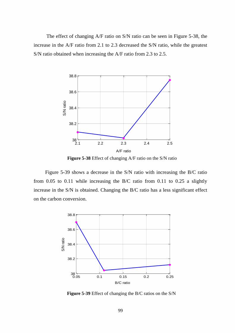
99
The effect of changing A/F ratio on S/N ratio can be seen in Figure 5-38, the
increase in the A/F ratio from 2.1 to 2.3 decreased the S/N ratio, while the greatest
S/N ratio obtained when increasing the A/F ratio from 2.3 to 2.5.
Figure 5-39 shows a decrease in the S/N ratio with increasing the B/C ratio
from 0.05 to 0.11 while increasing the B/C ratio from 0.11 to 0.25 a slightly
increase in the S/N is obtained. Changing the B/C ratio has a less significant effect
on the carbon conversion.
2.1 2.2 2.3 2.4 2.538
38.2
38.4
38.6
38.8
A/F ratio
S/N
ratio
0.05 0.1 0.15 0.2 0.2538
38.2
38.4
38.6
38.8
B/C ratio
S/N
ratio
Figure 5-38 Effect of changing A/F ratio on the S/N ratio
Figure 5-39 Effect of changing the B/C ratios on the S/N
ratio

100
To check the trends of the mean S/N ratios with different levels of the studied
variables the mean carbon conversion has been calculated with the three different
levels and the results can be shown in Appendix F.
The best experimental conditions can be concluded from the previous
figures and from figures F-1, F-2, F-3, and F-4. The arithmetic value of the
maximum point in each graph indicates the best choice of the experimental
conditions. Therefore, the best conditions for the largest carbon conversion are A
Steam to fuel (S/F) ratio at level 3 (0.75), B Air to fuel (A/F) ratio at level 3 (2.5), C
Biomass to coal (B/C) ratio at level 1 (0.05), and D Temperature, °C at level 3 (850
°C). In other words, the best experimental conditions are A3, B3, C1, and D3 in
Table 5-3.
5.4.3 Effect of different variable levels on the average gas
compositions
The gas produced form coal-garape seeds gasification contains CO2, CO, H2,
CH4 and less composition of the minor components (C2H2, C2H4, C2H6, H2S, COS,
C3H6, and C3H8) reaches to about 0.004-0.0075. In this part the obtained average
composition of CO2, CO, H2, and CH4 will be discussed.
Figure 5-40 shows the average compositions of CO2, CO, H2, and CH4
obtained when changing the A/F ratio. Increasing the A/F ratio rom 2.1 to 2.3 led to
increase the molar average composition of CO. Reaction 1 is more favourable than
reaction 3 as it is less exothermic which explains the increase of CO and the
decrease in CO2. Further increase in A/F ratio from 2.3 to 2.5 the reverse trend will
happen; CO will decrese and CO2 will increase that happens due to increase
reaction 2 and 3 producing more CO2 and consming the excess of CO in the gasifier
and the decrease in the produced CO can explaine the increase in hydrogen
composition by reaction 5. Methane composition will increase from A/F of 2.3 to
2.5 as it is mailnly dependent on hydrogen compositions.

101
Figure 5-41 shows the average compositions of CO2, CO, H2, and CH4
formed at different levels of S/F. A slighlt decrease in the average molar
compositions is noticed with an increase the ratio of S/F from 0.25 to 0.5 while
increasing the S/F from 0.5 to 0.75 causes the average molar compositions of CO2
and H2 to increase that explains reaction 5 is more rapid at higher S/F ratios. CO
and CH4 are slightly decreased due to their consumption by reaction 5 and 8
producing more hydrogen and carbon dioxide.
2.1 2.15 2.2 2.25 2.3 2.35 2.4 2.45 2.50
0.05
0.1
0.15
0.2
A/F ratio
avera
ge g
as c
om
positio
n
H2
CO2
CO
CH4
0.3 0.4 0.5 0.6 0.70
0.02
0.04
0.06
0.08
0.1
0.12
0.14
S/F ratio
avera
ge g
as c
om
positio
n
H2
CO2
CO
CH4
Figure 5-40 Effect of A/F ratio on the average gas compositions
Figure 5-41 Effect of S/F ratio on the average gas compositions

102
Figure 5-42 shows the average molar compositions of the produced carbon
monoxide, carbon dioxide, hydrogen, and methane with changing the bed
temperature. All the producer gas components obtained increased with temperature
increase. The maximum increase for CO, H2, and CH4 achieved at a bed
temperature increase from 820 °C to 850 °C, at higher bed temperatures the
endothermic reaction will be higher than the exothermic reactions, therefore higher
CO and H2 will be produced by reactions 6, 7, and 8 while decreasing CO2 is due to
its consumption by reaction 6 producing more CO.
Figure 5-43 shows the values of the average composition of CO2, CO, H2, and
CH4 results with varying the B/C ratio at different levels. Both hydrogen and carbon
monoxide decreased from B/C ratio of 0.05 to 0.11 and then slgihtly increase in
hydrogen composition and slightly decreased in carbon monoxide composition have
been occurred when increasing the B/C ratio from 0.25 to 0.5. While the
compositions of carbon dioxide and methane are shown to increase with increasing
B/C ratio and the maximum average composition obtained with an increase from
0.11 to 0.25. The increase in CO2, CH4, and H2 is due to burning more carbon by
reactions 3, 4, and 7 respectively, the produced CO by reaction 1 and 6 will be
800 810 820 830 840 8500
0.02
0.04
0.06
0.08
0.1
0.12
0.14
Temperature, C
avera
ge g
as c
om
positio
n
H2
CO2
CO
CH4
Figure 5-42 Effect of bed temperature on the average gas compositions

103
consumed by reaction 2 producing CO2 and reaction 5 producing CO2 and H2 which
explains the increase in CO2 and H2 and the decreased in CO composition.
0.05 0.1 0.15 0.2 0.250
0.02
0.04
0.06
0.08
0.1
0.12
0.14
B/C ratio
avera
ge g
as c
om
positio
n
H2
CO2
CO
CH4
Figure 5-43 Effect of B/C ratio on the average gas compositions

104
5.5 Theoretical modelling
5.5.1 Distribution of gas compositions in the gasifier
The gases concentrations in axial direction along the bed height were
obtained by solving Equations 3.15, 3.17, and 3.24 numerically using finite
difference method. The model calculates the gas concentration profile of O2, CO2,
CO, H2, and H2O in the spout and annulus regions as a function of the bed height.
The theoretical gas concentration profiles were compared against the experimental
values of coal gasification process to examine the accuracy of the predicted model.
The calculations were performed for constant bed temperature during the
experiment of 850 °C, coal flow rate of 1.6 kg/h with steam to fuel ratio of 0.75.
Figure 5-44 shows the profile of oxygen concentration in the spout and
annulus regions obtained theoretically and compared with experimental results. It
can be noticed that oxygen is consumed rapidly in both regions but at different
rates, oxygen composition in the spout at the bed exit is 0.0061 in the annulus and
in the bed exit it is 0.0021. The fast depletion of oxygen concentration is due to the
combustion reactions that are happening fast at the gasifier inlet producing carbon
dioxide and carbon monoxide. The average experimental composition of the oxygen
at the bed exit is 0.0045 where the average calculated composition from the
predicted model is equal to 0.0041.

105
Figure 5-45 shows the concentration profile of carbon dioxide in the spout
and in the annulus regions and the average experimental composition of carbon
dioxide at the bed exit. Carbon dioxide composition increased rapidly in both spout
and annulus regions, and it‘s value in the spout is higher than that in the annulus
which indicates that complete oxidation is happening at the spout region and it is an
exothermic region because the more exothermic reactions is happening at the spout
region, so combustion reactions occurs in the spout producing more carbon dioxide.
The value of carbon dioxide concentration at the bed exit in the spout region is
0.1959 and it‘s value at the bed exit in the annulus region is 0.162, while the
average experimental concentration of carbon dioxide is 0.198.
Figure 5-44 Theoretical concentration profiles for oxygen in the spout and the annulus

106
Figure 5-46 shows the composition profile of carbon monoxide with the bed
height in the gasifier in both spout and annulus regions. It can be noticed from
Figure 5-45 that complete oxidation happens at the spout region forming carbon
dioxide, so the rest of oxygen will be consumed in the partial oxidation reaction
forming carbon monoxide and that explains the excess amount of carbon monoxide
in the annulus region. The value of CO composition at the bed exit in the annulus
region is 0.14 while it‘s value at the bed exit in the spout region is 0.06. The
average experimental composition of CO at the bed exit is 0.108.
Figure 5-45 Theoretical concentration profiles for carbon dioxide in the spout and the
annulus

107
Figure 5-47 shows the theoretical composition profile for steam with the bed
height in the spout and annulus regions. The steam is almost consumed rapidly in
both regions but at different rates; more rapidly in the annulus than in the spout and
it is molar composition at the bed exit in the spout region is Nil, while it is
composition at the bed exit in the annulus is Nil, and no steam is recorded in the
experimental work. These trends suggest that the spout tends to be an oxidizing
exothermic which is the same conclusion obtained from Figure 5-45, while the
annulus behaves as a reducing endothermic region.
Figure 5-46 Theoretical concentration profiles for carbon monoxide in the spout and
the annulus

108
Figure 5-48 shows the profile of hydrogen composition with the bed height in
the spout and annulus regions. The composition of hydrogen at the bed exit in the
spout region is 0.165 where it is value at the bed exit in the annulus region is 0.2.
Because annulus region behaves as endothermic region, the steam will be consumed
and endothermic reactions will increase producing more hydrogen and carbon
monoxide in the annulus region. The average experimental hydrogen composition is
obtained at the same conditions is 0.192.
Figure 5-47 Theoretical concentration profiles for steam in the spout and the annulus

109
5.5.2 Comparison of Experimental and Isothermal Model results
The results from the isothermal model are compared with the experimental
results obtained when running the gasifier with the same operating conditions.
Table 5-6 shows the composition of the gases at the bed exit in both annulus and
spout region and the average experimental composition at the bed exit. The average
calculated gas compositions in Table 5-6 represent the average composition of each
gas results from the spout and annulus regions at the bed exit.
Table 5-6 Theoretical and experimental producer gas compositions at the bed exit
Gas
components
Gas composition Average gas composition % Error
Annulus Spout Calculated Experimental
O2 0.0021 0.0061 0.0041 0.0045 9.75609756
H2 0.2 0.165 0.1825 0.192 5.20547945
CO 0.14 0.06 0.1 0.108 8
CO2 0.1959 0.162 0.17895 0.198 10.6454317
Figure 5-49 shows comparison between the average compositions at the bed
exit obtained from the isothermal model and the average experimental compositions
Figure 5-48 Theoretical concentration profiles for hydrogen in the spout and the
annulus.

110
for the producer gas components at the same operating conditions of 850 °C bed
temperature, 0.75 steam to fuel ratio, and 1.6 kg/h fuel rate.
Figure 5-49 Experimental and theoretical concentration profiles for CO2, CO, H2, and O2
at the bed exit.
The above figure shows good agreement between the results obtained from
the experiment and the results from the theoretical isothermal model. The % error
between the average experimental and the average theoretical compositions is
calculated from the following equation:
(5.8)
5.5.3 Checking the validity of the predicted isothermal Model
The validity and accuracy of the proposed isothermal model for gasification
process using MATLAB (R2011a) are checked with the results obtained by Lucas
et al., (1991) when using the same operating conditions of 925 °C bed temperature,
0.305 m column diameter, 0.61 m bed height, 0.00162 m particle diameter, and
27.50 kg/h coal feed rate. Table 5-7 shows the compositions of CO, CO2, and H2
obtained by Lucas et al., (1991) and the compositions of these gases results from
the completed isothermal model when using the same operating conditions. Figure
5-50 shows the comparison between the results obtained from the isothermal model
0
0.05
0.1
0.15
0.2
0.25
O2 H2 CO CO2
ga
s m
ola
r co
mp
osi
tio
n
gas components
Calculated
Experimental

111
and the results obtained from Lucas et al., (1991) in both annulus and spout regions
at the bed exit.
Table 5-7 Producer gas compositions at the bed exit results from the completed model and
the compositions obtained by Lucas et al., (1991) model.
Gas
components
Complete
model,
spout
Lucas et
al., spout
Complete
model,
annulus
Lucas
et al.,
annulus
Complete
model,
average
Lucas et
al.,
average
% Error
CO 0.031 0.018 0.127 0.1186 0.079 0.0683 13.5443038
CO2 0.162 0.1752 0.143 0.1512 0.1525 0.1632 7.01639344
H2 0.053 0.0432 0.09124 0.0859 0.07212 0.06455 10.4963949
Figure 5-50 CO, CO2, and H2 concentration at the bed exit in both annulus and spout
regions resulting from the completed model and Lucas et al., (1991) model.
Figure 5-51 shows the comparison between the average compositions for
CO, CO2, and H2 at the bed exit in both annulus and spout regions obtained from the
completed model and results obtained from Lucas et al., (1991) model. Good
agreement can be noticed between the results obtained from the isothermal model
and that obtained by Lucas et al., (1991), 13.544% error for carbon monoxide
compositions, 7.016% error for carbon dioxide compositions, and 10.496% error for
hydrogen compositions.
0
0.02
0.04
0.06
0.08
0.1
0.12
0.14
0.16
0.18
0.2
CO CO2 H2
gas
mo
lar
com
po
siti
on
gas components
complete model,spout
Lucas et al.,spout
complete model,annulus
Lucas et al.,annulus
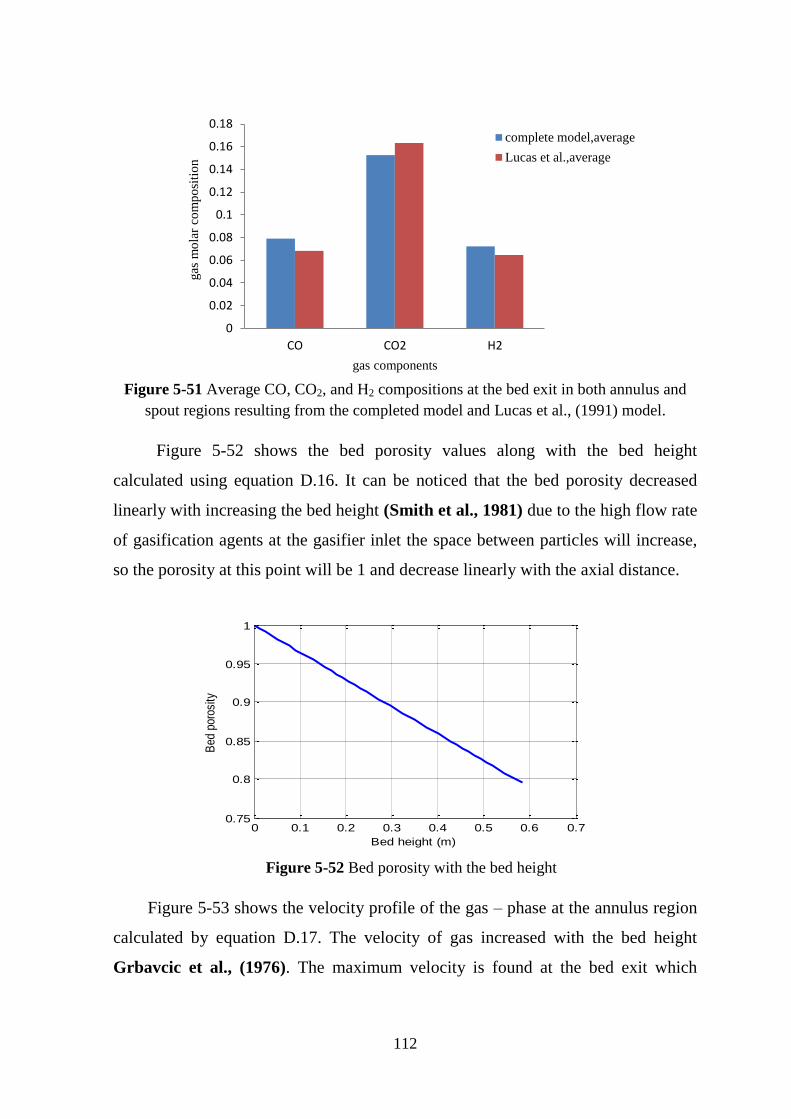
112
Figure 5-51 Average CO, CO2, and H2 compositions at the bed exit in both annulus and
spout regions resulting from the completed model and Lucas et al., (1991) model.
Figure 5-52 shows the bed porosity values along with the bed height
calculated using equation D.16. It can be noticed that the bed porosity decreased
linearly with increasing the bed height (Smith et al., 1981) due to the high flow rate
of gasification agents at the gasifier inlet the space between particles will increase,
so the porosity at this point will be 1 and decrease linearly with the axial distance.
Figure 5-53 shows the velocity profile of the gas – phase at the annulus region
calculated by equation D.17. The velocity of gas increased with the bed height
Grbavcic et al., (1976). The maximum velocity is found at the bed exit which
0
0.02
0.04
0.06
0.08
0.1
0.12
0.14
0.16
0.18
CO CO2 H2
gas
mo
lar
com
po
siti
on
gas components
complete model,average
Lucas et al.,average
0 0.1 0.2 0.3 0.4 0.5 0.6 0.70.75
0.8
0.85
0.9
0.95
1
Bed height (m)
Bed
por
osity
Figure 5-52 Bed porosity with the bed height

113
explains the trend of gasification agent motion because when entering the gasifier
most of it will be in the spout and at the top of the spout region the solid particles
will move on the annulus sides. This movement of particles may cause motion for
the gasification agent and the velocity of gas will be high due to the high number of
solid particles entering the annulus region.
0 0.1 0.2 0.3 0.4 0.5 0.6 0.70
2
4
6
8
10
12
14
Bed height (m)
Gas a
nnulu
s v
elo
city (
m/s
)
Figure 5-53 Gas – phase velocity profile at the annulus region
114
Chapter Six
Conclusions and Recommendations
6.1 Conclusions
From the present work the effect of temperature, A/F ratio and S/F ratio on the
composition of producer gas generated from coal, algae, coal-algae, and coal-grape
seeds gasification processes in a 77 mm inside diameter spouted bed gasifier was
investigated. The following conclusions can be drawn:
1. The average molar concentration of hydrogen obtained from coal gasification
increases with increasing bed temperature to 850 °C.
2. At lower coal feed rate of 1.28 kg/h, the composition of the produced CO2
decreases while that of CO and CH4 increases with bed temperature increase.
Increasing the coal feed rate to 1.43 and 1.6 kg/h results in considerable
increase in the compositions of the produced CO2, CO, and CH4.
3. Operating without steam leads to an increase in the bed temperature to
unstable high limit which is sometimes referred to as the ―sintering point‖.
Above the sintering point, bed agglomeration occurred.
4. Agglomeration is prevented by using (air-steam) gas mixture as a gasification
agent. Injection of steam through the gasifier with a S/F ratio of 0.5 or 0.75
decreased the bed temperature due to the energy consumption for water
evaporation.
5. The average molar concentrations of CO2, H2 and CH4 increase when
increasing the ratio of steam to fuel from 0.5 to 0.75, while CO average molar
concentrations decreases.
6. Operating the gasifier with 820 °C bed temperature the average molar
concentrations of the produced hydrogen increased with increasing the ratio
of A/F, while at 850 °C the average concentrations of hydrogen decreased
with increasing the A/F ratio.

115
7. The conversion of carbon increases with increasing mass rate of coal, bed
temperature, and S/F ratio the maximum value of carbon conversion obtained
is 92.9% at 1.8 A/F ratio, 850 °C bed temperature, and 0.75 S/F ratio.
8. Gasification of unleached algae results in bed agglomeration, apparently due
to the high salt content of the raw algae. Leaching of raw algae is required to
dissolve the salt content.
9. Co-gasification of coal-grape seeds with the same operating conditions
applied with coal gasification results in the formation of molten potassium
and sodium silicate which is accumulated with time stopping fluidization.
Avoiding the formation of molten components achieved by increasing the
A/F ratio.
10. According to the Taguchi method in design experiment of coal-grape seeds
gasification the bed temperature is the most influential parameter on the
carbon conversion while the ratio of B/C has low effect on carbon conversion
and the best experimental conditions are 850 °C bed temperature, 0.75 S/F
ratio, 2.5 A/F ratio, and 0.05 B/C ratio. For best conditions the carbon
conversion is 96.1%.
11. Spout-fluid bed gasification is suitable for hydrogen production.
12. According to the isothermal model more carbon dioxide produced in the
spout region while carbon monoxide and hydrogen produced more at the
annulus region. These trends suggest that the spout tends to be an oxidizing
exothermic region, while the annulus behaves as a reducing endothermic
region. Good agreement is obtained between the experimental results and the
isothermal model results.
116
6.2 Recommendations for the future work
The following suggestions for future work can be considered:
1. Increase the production of hydrogen for fuel cells by steam gasification of
different biomass types and by using catalysts such as ZnCl2 and dolomite.
2. Study the mechanisms of gasification reactions at high pressure and at
different A/F ratios.
3. Feed the fuel nearer to the bed and increasing the height of column in algae
gasification experiments to avoid the fuel elutriation and downstream gas
outlet blockages.

117
References
Abadie, L.M., and Chamorro, J.M., ―The Economics of Gasification: A Market-
Based Approach‖. Energies Journal, Vol. 2, 662-694; doi:
10.3390/en20300662, August (2009).
Abdullah, S., and Yusup, S.,‖ Method for screening of Malaysian biomass based on
aggregated matrix for hydrogen production through gasification‖. Journal of
applied sciences 10, 3301-3306, (2010).
Abdul Salam, P., and Bhattacharya, S.C., ―A comparative hydrodynamic study of
two types of spouted bed reactor designs‖. Chemical Engineering Science
61, 1946 – 1957, doi:10.1016/j.ces.2005.10.044, (2006).
Abdul Salam, P., S., Kumar, and Siriwardhana, M., ―Report on the status of
biomass gasification‖. October (2010).
Agency, I.E., World Energy Outlook Executive Summary, (2011).
Ammar, S. H., ―Hydrodesulfurization of thiophene over Co-Mo/AlO catalyst using
fixed-and fluidized-bed reactors‖. PHD thesis, Baghdad university, (2009).
Arnavat, M., P., Bruno, J., C., and Coronas, A., ―Review and analysis of biomass
gasification models‖. Renewable and Sustainable Energy Reviews 14, 2841–
2851, doi:10.1016/j.rser.2010.07.030, (2010).
Basu, P., ―Combustion and Gasification in Fluidized Beds-CRC Press.‖. ISBN 0-
8493- 3396 2, 456 pages, (2006).
Belgiorno, V., Feo, G. De, Della Rocca, C., and Napoli, R.M.A., ―Energy from
gasification of solid wastes‖. Science direct Journal, 23, 1-15, (2002).
Berkman, J., A., H., and Michael, G., ―ALGAL BIOMASS‖. Ebook, Chapter A7,
Biological Indicators Algal Biomass Indicators, Version 1.0 (2007).
Biba, V., Macak, J., Klose, E., Malecha, J., Ind. Eng. Chem. Proc. Des. Dev.17, 92–
98, (1978) as sign in Mendes et al., (2008).
Boateng, A. A., Walawender, W. P., Fan, L.T. and Chee, C.S., ―Fluidized bed
gasification of rice hull‖. Bioresource Technology, 40(3): 235-239, (1992).
118
Bourgeois, P., Grenier, P., ―The ratio of terminal velocity to minimum fluidising
velocity for spherical particles‖. Canadian Journal of Chemical Engineering,
Volume 46, Issue 5, pages 325–328, October (1968).
Bridgwater, A.V., Evans, G.D., ―An Assessment of Thermochemical Conversion
Systems for Processing Biomass and Refuse‖. Energy Technology Support
Unit (ETSU) on behalf of the Department of Trade, ETSU B/T1/00207/REP,
(1993).
Brown, J., ―Biomass Gasification: Fast Internal Circulating Fluidised Bed Gasifier
Characterisation and Comparison‖. Master thesis in Chemical and Process
Engineering, University of Canterbury, (2006).
Brunello, G., Nina, G.D., Nunes, and F.C.S., Nascimento, C.A.O., ―Minimum air
requirement for spouting mixed particles‖. Canadian Journal of Chemical
Engineering 52, 170–173, (1974).
Campbell, M., N., ―Biodiesel: Algae as a Renewable Source for Liquid Fuel‖.
Guelph Engineering Journal, (1), 2 - 7. ISSN: 1916-1107, (2008).
Cao, Y., Wang, Y., Rieley, J. and Pan, W., ―A novel biomass air gasification
process for producing tar-free higher heating value fuel gas‖. Fuel Processing
Technology, Vol. 87, 4, 343-353, (2005).
Carlozz, P., ―Closed Photobioreactor Assessments to Grow, Intensively, Light
Dependent Microorganisms: A Twenty-Year Italian Outdoor Investigation‖.
The Open Biotechnology Journal, 2, 63-72, (2008).
Carlsson, A., S., Beilen, J., B., V., Ralf, M., and Clayton, D., ―UTILITY FOR
INDUSTRIAL APPLICATIONS‖. Outputs from the EPOBIO project,
CNAP, University of York, September (2007).
Chatterjee, P., K., Datta, A., B., and Kundu, K., M., ―Fluidized bed gasification of
coal‖. The Canadian Journal of Chemical Engineering, Vol. 73, Issue 2,
pages 204–210, 1995, DOI: 10.1002/cjce.5450730206, published MAR,
(2009).
Choi, M., and Meisen, A., ―Hydrodynamics of shallow, conical spouted beds‖. The
Canadian Journal of Chemical Engineering 70, 916–924, (1992).

119
Chopra, S. and A. Jain, ―A Review of Fixed Bed Gasification Systems for
Biomass‖. Agricultural Engineering International: the CIGR Ejournal, Vol.
IX, April, (2007).
Ciferno, J. P., and Marano, J. J., ―Benchmarking Biomass Gasification
Technologies for Fuels, Chemicals and Hydrogen Production‖. June (2002).
Craig, K., R., and Margaret, K., M., ―Cost and Performance Analysis of Biomass-
Based Integrated Gasification Combined-Cycle (BIGCC) Power Systems‖.
DE-AC36-83CH10093, NREL/TP-430-21657, October (1996).
Darby, R., ―Chemical engineering fluid mechanics‖. ISBN: 0-8247-0444-4, (2001).
Deng, Z., Xiao, R., Jin, B., Huang, H., Shen, L., Song, Q., and Li, Q.,
―Computational Fluid Dynamics Modeling of Coal Gasification in a
Pressurized Spout-Fluid Bed‖. Energy & Fuels, 22, 1560–1569, (2008).
Di, B., C., ―Dynamic behaviour of stratified downdraft gasifier‖. Chemical
Engineering Science 55, 2931–2944, (2000).
Dixit, R., and Shivanand P., ―Fluidization Technologies: Aerodynamic Principles
and Process Engineering‖. Journal of Pharmaceutical sciences , VOL. 98,
NO. 11, Wiley InterScience, DOI 10.1002/jps.21722, April (2009).
Dogan, O. M., UYSAL B. Z. & GRACE J. R., ―HYDRODYNAMIC STUDIES IN
A HALF SLOT-RECTANGULAR SPOUTED BED COLUMN‖. Chem.
Eng. Comm., 191: 566_579, 2004, ISSN: 0098-6445 print/1563-5201online,
DOI: 10.1080/00986440490277992, (2004).
Du, W., Bao, Xu, X. J., and Wei, W., ―Computational fluid dynamics (CFD)
modeling of spouted bed: Assessment of drag coefficient correlations‖.
Chemical Engineering Science 61, 1401–1420,
doi:10.1016/j.ces.2005.08.013, (2006).
Eliasson, B., and Taylor, G., ―The Future of the Hydrogen Economy: Bright or
Bleak?‖, ereport, www.efcf.com/reports, February (2005).
Eng, J. H., Svrcek, W., Y., and Behie, L., A., ―Dynamic Modeling of a Spouted Bed
Reactor with a Draft Tube‖. Ind. Eng. Chem. Res., Vol. 28, No. 12, (1989).

120
Ergudenler, A., ―Gasification of Wheat Straw in a Dual-Distributor Type Fluidized
Bed Reactor‖. Ph.D. Thesis, Technical University of Nova Scotia, Nova
Scotia, Canada, (1993).
Eyk, P., J., V., Kosminski, A., and Ashman, P., J., ―Control of Agglomeration and
Defluidisation during Fluidised Bed Combustion of South Australian Low-
Rank Coals‖. Energy and Fuels Journal, DOI: 10.1021/ef2011518, (2011).
Eyk, P., J., V., Muhlack, R., A., and Ashman, P., A., ―Gasification of Grape Marc in
a Circulating Fluidised Bed‖. Proceedings of the Australian Combustion
Symposium, the University of Queensland, December, (2009).
Fogler, H., S., ―Element of chemical reaction engineering‖. Third edition, (1999).
Gao, Y., Gregor., C., Liang, Y., Tang, D., and Tweed C., ―Algae Biodiesel‖. A
Feasibility Report, BPRO 29000, (2009).
Geankoplis, C., J., ―Transport processes and unit operations‖. Third edition, ISBN
0-13-045253-X, (1993).
Global bioenergy partnership, ―ALGAE-BASED BIOFUELS: A Review of
Challenges and Opportunities for Developing Countries‖. (2009).
Goldemberg, J., ―The Case for Renewable Energies‖. Thematic Background Paper,
February (2004).
Gonzáleza, J., F., Román, S., Bragado, D., and Calderón, M., ―Investigation on the
reactions influencing biomass air and air/steam gasification for hydrogen
production‖. Fuel processing technology 89, 764- 772, (2008).
Grace, J.R., In: Hetsroni, G. (Ed.), Handbook of Multiphase Systems. Hemisphere,
New York, Chapter 8, (1982).
Grbavcic, Z., B., VukoviC D. V., Zdaaski F. K. and Littman H., Can. J. Chem.
Engng 54 3, (1976).
Greenwood N. N., Earnshaw A., Chemistry of the Elements, Pergamon Press,
Oxford, United Kingdom, (1984).
Heiskanen, L., ―A study on rate correlations of gasification reactions‖.
Lappeenranta University of Technology Faculty of Technology Degree
Program of Energy Technology, (2011).
121
Hook, B., D., H. Littman, M.H. Morgan III, Y. Arkun, and Can. J. Chem. Eng. 70,
966–982, (1992) as sign in Mendes et al., (2008).
Höök, M., ―Coal fundamentals A brief overview‖, (2007).
Hoque, M. M., Bhattacharya S., C., ―Fuel characteristics of gasified coconut shell in
a fluidized and a spouted bed reactor‖. Energy, 26, pp101–10, (2001).
Hsu, D., D., ―Life Cycle Assessment of Gasoline and Diesel Produced via Fast
Pyrolysis and Hydroprocessing‖. Technical Report, March (2011).
Jackson, R. and Judd, M. R., Trans IChemE, 59, 119, (1981).
Jin, H., Lu, Y., Liao, B., Guo, L., and Zhang, X., ―Hydrogen production by coal
gasification in supercritical water with a fluidized bed reactor‖. International
Journal of Hydrogen Energy, 35, 7151- 7160, (2010).
Knoef, I. H. A. ―BTG Biomass Gasification‖. April (2008).
Kong, L., L., G., ZHANG, B., HE, W., and WANG, H., ―Hydrogen Production
from Biomass Wastes by Hydrothermal Gasification‖. Energy Sources, Part
A, 30:1166–1178, Taylor & Francis Group, LLC, ISSN: 1556-7036
print/1556-7230 online, DOI: 10.1080/15567030701258246, (2008).
Kreith, F., Boehm, R.F., ―Heat and Mass Transfer‖. Mechanical Engineering
Handbook, (1999).
Lettner, F., T., Helmut, H., Peter, ―Biomass gasification – State of the art
description‖. Graz University of Technology - Institute of Thermal
Engineering, Grant agreement no EIE/06/078/SI2.447511, December (2007).
Lim, C., J., M., Sulaiman, H., and A., P., Watkinson, Can. J. Chem. Eng. 69, 596–
606, (1991).
Lim, M. T., and Alimuddin, Z., ―Bubbling fluidized bed biomass gasification-
Performance, process findings and energy analysis‖. Science direct Journal,
33, 2339–2343, (2008).
Limtrakul, S., Chalermwattanatai, A., Unggurawirote, K., Tsuji, Y., Kawaguchi, T.,
Tanthapanichakoon, W., ―Discrete particle of solids motion in a gas–solid
fluidized bed‖. Chemical Engineering Science 58, 915–921, (2003), as sign
in Limtrakul, S., Boonsrirat, A., and Vatanatham, T., ―DEMmodeling and
122
simulation of a catalytic gas–solid fluidized bed reactor: a spouted bed as a
case study‖.
Li, Q., Zhang, M., Zhong, W., Wang, X., Xiao, R., and Jin, B., ―Simulation of Coal
Gasification in a Pressurized Spout-Fluid Bed Gasifier‖. The Canadian
Journal of chemical engineering, vol 87, April (2009).
Littman , H., P.V. Narayan, A.H. Tomlins, and M.L. Friedman, AIChE Symposium
Series, vol. 77, 174–180, (1981).
Li, X.T., Grace, J.R., Lim, C.J., Watkinson, A.P., Chen, H.P., and Kim, J.R.,
―Biomass gasification in a circulating fluidized bed‖. Biomass and
Bioenergy 26, 171 – 193, doi:10.1016/S0961-9534(03)00084-9, (2004).
Lucas, A., Arnaldos, J., Casal, J., and Puigjaner, L., ―Improved equation for
calculation of minimum fluidization velocity‖. Industrial & Engineering
Chemistry Process Design and Development 25, 426–429, (1986).
Lucas, J.P., Lim, C.J., and Watkinson, A.P., ―A nonisothermal model of a spouted
bed gasifier‖. Fuel Vol. 77, No. 7, pp. 683-694, PII:S OO16-2361(97)00237,
(1998).
Lucas, J. P., Watkinson, A. P. and Lim, C. J., ―Mathematical Model of C.R.E.
Gastjier‖. Report of Contract CREICON 1035 to British Coal Corporation,
(1991) as sign in Lucas et al., (1998).
Lv, P., Chang, J., Xiong, Z., Huang, H., Wu, C., and Chen, Y., ―Biomass Air-Steam
Gasification in a Fluidized Bed to Produce Hydrogen-Rich Gas‖. Energy and
Fuels, 17, 677-682, (2003).
Mahamuni, N.N. and Adewuyi, Y.G.. ―Application of Taguchi Method to
Investigate the Effects of Process Parameters on the Transesterification of
Soybean Oil Using High Frequency Ultrasound‖. Energy Fuels, 24, 2120-
2126, (2010).
Mamuro, T., and Hattori, H., J. Chem. Engng Japan (1968) as sign in Mendes et al.,
(2008).
Matsui, D. K., Furusawa T., Chem. Eng. J. 18, 105–113, (1985) as sign in Mendes
et al., (2008).

123
Matsui I., Kunii D., Furusawa T., Ind. Eng. Chem. Res. 26, 91–95, (1987) as sign in
Mendes et al., (2008).
Mathur, K.B., and Gishler, P.E., ―A technique for contacting gases with coarse solid
particles‖. A.I.Ch.E. Journal 1, 157–164, (1955).
Mathur, K.B., Gishler, P.E., ―A technique for contacting gases with coarse solid
particles‖. A.I.Ch.E. Journal 1 (1), 157–164, (1955).
McCullough D. P., Eyk P. J., Ashman P. J., and Mullinger, ―Investigation of
Agglomeration and Defluidization during Spouted-Bed Gasification of High-
Sodium, High-Sulfur South Australian Lignite‖. Chemical engineering
department, University of Adelaide, (2011).
Mendes, A., Dollet, A., Ablitzer, C., Perrais, C., and Flamant, G., ―Numerical
simulation of reactive transfers in spouted beds at high temperature:
Application to coal gasification‖. Science direct journal, 82, 117–128,
doi:10.1016/j.jaap.2008.02.001, (2008).
Mermoud, F., Golfier, F., Salvador, S.,Van de Steene and J Dirion, ―Experimental
and numerical study of steam gasification of a single charcoal particle‖.
Combustion and Flame 145 (2006) 59–79, (2006).
Narvaez, I., Orıo, A., Aznar, M. P., and Corella, J.,‖ Biomass Gasification with Air
in an Atmospheric Bubbling Fluidized Bed. Effect of Six Operational
Variables on the Quality of the Produced Raw Gas‖, Ind. Eng. Chem. Res.,
35, 2110-2120,( 1996).
Neogi D., Chang C.C., W.P., and Walawender L.T., ―Study of coal gasfication in an
experimental fluidized bed reactor‖. AlChE Journal (Vol. 32, No. 1), January
(1986).
Olazar, M., San Josh, M. J., Aguayo, A., T., Arandes, J., M., and Bilbao, J., ―Design
Factors of Conical Spouted Beds and Jet Spouted Beds‖. Znd. Eng. Chem.
Res., 32, 1245-1250, (1993).
Palacio, D., L., and Philippe B., ―Hydrogen Energy and Fuel Cells‖. Final report of
the high level group, EUROPEAN COMMISSION, (2003).

124
Purdy, M., J., Felder, R., M., and Ferrell, J., K., ―Coal Gasification in a Pilot Scale
Fluidized Bed Reactor, Gasification of a New Mexico Subbituminous Coal‖.
Ind. Eng. Chem. Process Des. Dev., 23, 287-294, (1984).
Rajvanshi, A., K., ―BIOMASS GASIFICATION‖. Director, Nimbkar Agricultural
Research Institute, PHALTAN-415523, Maharashtra, India, (Published as a
Chapter (No. 4) in book ―Alternative Energy in Agriculture‖. Vol. II, Ed. D.
Yogi Goswami, CRC Press, 83-102, (1986).
Riis, T., Elisabet, F., H., Vie, P., J., S., and Ulleberg, Q., ―HYDROGEN
PRODUCTION AND STORAGE‖. INTERNATIONAL ENERGY
AGENCY, OECD/IEA, (2006).
Roos,C., J., ―Biomass Drying and Dewatering for Clean Heat & Power‖. WSU
Extension Energy Program, September (2008).
Sadaka, S. S., Ghaly, A. E., and Sabbah, M.A., ―Two-phase biomass air-steam
gasi_cation model for fluidized bed reactors: Part III—model validation‖.
Biomass and Bioenergy, 22 479 – 487, (2002).
Saito M., Sadakata M., Sakai T., Combust. Sci. Technol. 51, 109–128, (1983) as
sign in Mendes et al., (2008).
Salam, P. A., and Bhattacharya, S., C., ―A comparative study of charcoal
gasification in two types of spouted bed reactors‖. Energy 31, 228–243,
doi:10.1016/j.energy.2005.01.004, (2006).
Sanchez, I., G., Mazza, G., Flamant, and D., Gauthier, Chem. Eng. Sci. 55, 193–
202, (2000), as sign in Mendes et al., (2008).
Secondary and Intermediate Energy Infobook, Project P.O. Box 10101, Manassas,
VA 20108 1.800.875.5029, (2011).
Smith, K., I., YAMAN, A., and HOWARD, L., ―STUDIES ON MODELING AND
CONTROL OF SPOUTED BED REACTORS-I REACTOR MODELING‖.
Department of Chemical Engineering and Environmental Engineering,
Rensselaer Polytechnic Institute, Troy, NY 12181, U.S.A, (1981).
Taglia, P., P.G., ―Biogas: Rethinking the Midwest's Potential‖. June (2010).

125
Taguchi, G. Introduction to Quality Engineering; UNIPUB/Kraus International:
White Plains, (1986), as sign in Mahamuni, N.N., et al., (2010).
Tannous, K., ―Contribution a letude hydrodynamique des lits fluidises de grosses
particles. These de doctorat‖. INP-Toulouse, France, (1993) as sign in Abdul
Salam and Bhattacharya (2006).
Tesner P.A., in: Proceedings of the Eighth Symposium on Combustion, p. 807,
(1960 as sign in Mendes et al., (2008).
Thamavithya, M., Sompop J., Animesh D., and Prabir B., ―Experimental study on
sawdust gasification in a spout–fluid bed reactor‖. Int. J. Energy Res. 2012;
36:204–217, DOI: 10.1002/er.1796, (2010).
The US Energy Information Administration (EIA), International Energy Outlook
(2009).
Thonglimp, V., Hiquily, N., Laguerie, C., ―Vitesse minimale de fluidisation et
expansion des couches fluidises par un gaz‖. Powder Technology 38, 233–
253, (1984).
Tillman, D.A., ―Biomass Combustion. Biomass: Regenerable Energy‖. John Wiley
and Sons, 203-219, (1987).
TOSUN, I., ―MODELLING IN TRANSPORT PHENOMENA‖. A Conceptual
Approach, (2002).
Turare, C., ―Biomass Gasification – Technology and Utilisation‖. ARTES Institute,
Glucksburg, Germany, (2002).
Uemaki, O.,Yamada, R., and Kugo, M., ―Particle segregation in a spouted bed of
binary mixtures of particles‖. Canadian Journal of Chemical Engineering 61,
303–307, (1983).
Wagner, L., ―Biodiesel from algae oil, research report‖. July (2007).
Wang Y., Kinoshita C.M., Solar Energy 51, 19–25, (1993) as sign in Mendes et al.,
(2008).
Weil, S.A., S.P. Nandi, D.V. Punwani and J.L. Johnson. ―Peat hydrogasification‖.
(1978).

126
Wellinger, A., ―Algal Biomass:Does it save the world?‖. Short reflections, Task 37,
April (2009).
Wen, C.Y., and Yu, Y.H., ―Mechanics of fluidization‖. Chemical Engineering
Progress Symposium Series No. 62, 100–111, (1966).
Wen, Z., and Michael B., J., ―Microalgae as a Feedstock for Biofuel Production‖.
College of Agriculture and Life Sciences, Virginia Polytechnic Institute and
State University, Publication 442-886, (2009).
Werther, J., ―Fluidized-Bed Reactors‖. Ullmann‘s Encyclopedia of industrial
chemistry, Hamburg University of Technology, Hamburg, Germany, DOI:
10.1002/14356007.b04_239.pub2, (2012).
Wu, S.W.M., Lim, C.J., Epstein, N., ―Hydrodynamics of spouted beds at elevated
temperatures‖. Chemical Engineering Communication 62, 251–268, (1987).
Xiao, R., Zhang, M., Jin, B., and Huang Y., ―High-Temperature Air/Steam-Blown
Gasification of Coal in a Pressurized Spout-Fluid Bed‖ Energy & Fuels, 20,
715-720, (2006).
Yang, W., C., ―Modification and re-interpretation of Geldart's classification of
powders‖. Science direct Journal, Powder Technology 171 (2007) 69–74,
DOI:10.1016/j.powtec.2006.08.024, (2006).
Yu, L., Lu, J., Zhang, X., and Zhang, S., ―Numerical simulation of the bubbling
fluidized bed coal gasification by the kinetic theory of granular flow
(KTGF)‖. Fuel 86, 722–734, doi:10.1016/j.fuel.2006.09.008, (2007).
Zedtwitz, P., V., and Steinfeld, A., ―Steam-Gasification of Coal in a Fluidized-
Bed/Packed-Bed Reactor Exposed to Concentrated Thermal
RadiationsModeling and Experimental Validation‖. Ind. Eng. Chem. Res.,
44, 3852-3861, (2005).
Zhang, Y., Xiao, J., and Shen, L.,‖ Simulation of Methanol Production from
Biomass Gasification in Interconnected Fluidized Beds‖. Ind. Eng. Chem.
Res., 48, 5351–5359, (2009).
Zhong, W., Rui , X., and Mingyao, Z., ―Experimental Study of Gas Mixing in a
Spout-Fluid Bed‖. Thermoenergy Engineering Research Institute, Southeast

127
University, Nanjing 210096, China, DOI 10.1002/aic.10708, Wiley
InterScience, (2005).

A-1
Appendix A
Experimental Data
A.1 Coal gasification experiments results
Table A-1 Experimental results for run with coal feed rate = 1.6 kg/h, S/F ratio= 0.5, and bed Temperature = 850 °C
Table A-2 Experimental results for run with coal feed rate = 1.6 kg/h, S/F ratio= 0.75, and bed Temperature = 850 °C
Components Time, h Average
Composition 1h 2h 3h 4h
C2H2 0.0026551 0.0046137 0.00425009 0.00378489 0.00382595
CO2 0.1896412 0.2092024 0.20066609 0.19413747 0.19841179
C2H4 0.0004137 0.0006825 0.00065435 0.00059865 0.0005873
Components Time, h Average
Composition 1h 2h 3h 4h
C2H2 0.0021362 0.0035514 0.0027808 0.0035304 0.0029997
CO2 0.1517318 0.1927576 0.1939561 0.1972645 0.1839275
C2H4 0.0004582 0.0005101 0.0004368 0.0005146 0.0004799
C2H6 0.0008112 0.0019456 0.0016342 0.0019577 0.0015872
H2S 6.531E-05 0.0068521 0.0072179 0.0072147 0.0053375
COS 0.0004554 0.0002952 0.0003867 0.0003171 0.0003636
C3H6 0.0004999 0.0007362 0.0006989 0.0007583 0.0006733
C3H8 0.0001731 0.0007097 0.000665 0.0007206 0.0005671
H2 0.1396301 0.1718334 0.1675075 0.1448823 0.1559633
O2 0.0061795 0.0043048 0.0079389 0.0062531 0.0061691
N2 0.5426092 0.4787862 0.492676 0.5133664 0.5068595
CH4 0.0107394 0.0171409 0.0136193 0.017053 0.0146381
CO 0.1051754 0.0839117 0.0935535 0.1052449 0.0969714
total 0.9606649 0.9633349 0.9830717 0.9990777 0.9765373
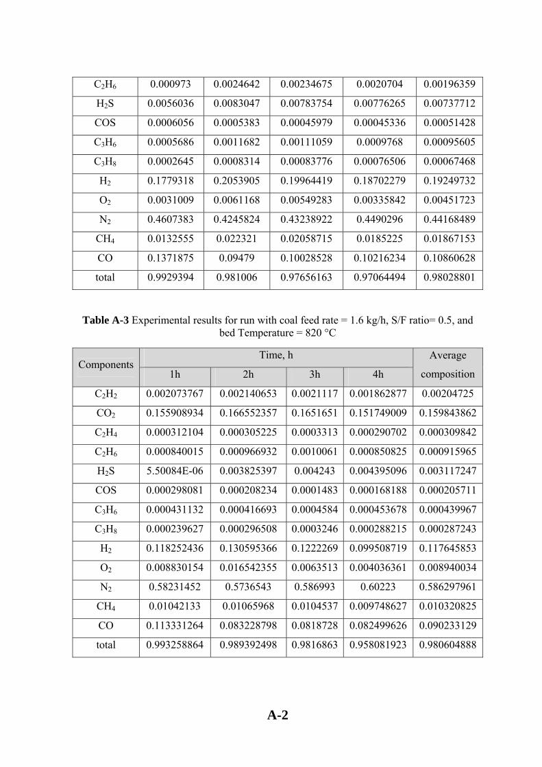
A-2
C2H6 0.000973 0.0024642 0.00234675 0.0020704 0.00196359
H2S 0.0056036 0.0083047 0.00783754 0.00776265 0.00737712
COS 0.0006056 0.0005383 0.00045979 0.00045336 0.00051428
C3H6 0.0005686 0.0011682 0.00111059 0.0009768 0.00095605
C3H8 0.0002645 0.0008314 0.00083776 0.00076506 0.00067468
H2 0.1779318 0.2053905 0.19964419 0.18702279 0.19249732
O2 0.0031009 0.0061168 0.00549283 0.00335842 0.00451723
N2 0.4607383 0.4245824 0.43238922 0.4490296 0.44168489
CH4 0.0132555 0.022321 0.02058715 0.0185225 0.01867153
CO 0.1371875 0.09479 0.10028528 0.10216234 0.10860628
total 0.9929394 0.981006 0.97656163 0.97064494 0.98028801
Table A-3 Experimental results for run with coal feed rate = 1.6 kg/h, S/F ratio= 0.5, and bed Temperature = 820 °C
Components Time, h Average
composition 1h 2h 3h 4h
C2H2 0.002073767 0.002140653 0.0021117 0.001862877 0.00204725
CO2 0.155908934 0.166552357 0.1651651 0.151749009 0.159843862
C2H4 0.000312104 0.000305225 0.0003313 0.000290702 0.000309842
C2H6 0.000840015 0.000966932 0.0010061 0.000850825 0.000915965
H2S 5.50084E-06 0.003825397 0.004243 0.004395096 0.003117247
COS 0.000298081 0.000208234 0.0001483 0.000168188 0.000205711
C3H6 0.000431132 0.000416693 0.0004584 0.000453678 0.000439967
C3H8 0.000239627 0.000296508 0.0003246 0.000288215 0.000287243
H2 0.118252436 0.130595366 0.1222269 0.099508719 0.117645853
O2 0.008830154 0.016542355 0.0063513 0.004036361 0.008940034
N2 0.58231452 0.5736543 0.586993 0.60223 0.586297961
CH4 0.01042133 0.01065968 0.0104537 0.009748627 0.010320825
CO 0.113331264 0.083228798 0.0818728 0.082499626 0.090233129
total 0.993258864 0.989392498 0.9816863 0.958081923 0.980604888
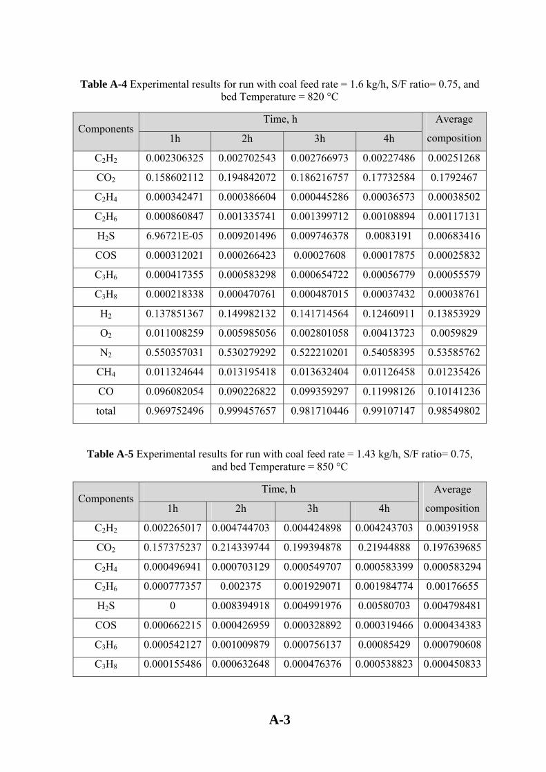
A-3
Table A-4 Experimental results for run with coal feed rate = 1.6 kg/h, S/F ratio= 0.75, and bed Temperature = 820 °C
Components Time, h Average
composition 1h 2h 3h 4h
C2H2 0.002306325 0.002702543 0.002766973 0.00227486 0.00251268
CO2 0.158602112 0.194842072 0.186216757 0.17732584 0.1792467
C2H4 0.000342471 0.000386604 0.000445286 0.00036573 0.00038502
C2H6 0.000860847 0.001335741 0.001399712 0.00108894 0.00117131
H2S 6.96721E-05 0.009201496 0.009746378 0.0083191 0.00683416
COS 0.000312021 0.000266423 0.00027608 0.00017875 0.00025832
C3H6 0.000417355 0.000583298 0.000654722 0.00056779 0.00055579
C3H8 0.000218338 0.000470761 0.000487015 0.00037432 0.00038761
H2 0.137851367 0.149982132 0.141714564 0.12460911 0.13853929
O2 0.011008259 0.005985056 0.002801058 0.00413723 0.0059829
N2 0.550357031 0.530279292 0.522210201 0.54058395 0.53585762
CH4 0.011324644 0.013195418 0.013632404 0.01126458 0.01235426
CO 0.096082054 0.090226822 0.099359297 0.11998126 0.10141236
total 0.969752496 0.999457657 0.981710446 0.99107147 0.98549802
Table A-5 Experimental results for run with coal feed rate = 1.43 kg/h, S/F ratio= 0.75, and bed Temperature = 850 °C
Components Time, h Average
composition 1h 2h 3h 4h
C2H2 0.002265017 0.004744703 0.004424898 0.004243703 0.00391958
CO2 0.157375237 0.214339744 0.199394878 0.21944888 0.197639685
C2H4 0.000496941 0.000703129 0.000549707 0.000583399 0.000583294
C2H6 0.000777357 0.002375 0.001929071 0.001984774 0.00176655
H2S 0 0.008394918 0.004991976 0.00580703 0.004798481
COS 0.000662215 0.000426959 0.000328892 0.000319466 0.000434383
C3H6 0.000542127 0.001009879 0.000756137 0.00085429 0.000790608
C3H8 0.000155486 0.000632648 0.000476376 0.000538823 0.000450833

A-4
H2 0.166571164 0.195136255 0.198917333 0.198722869 0.189836905
O2 0.011837868 0.004249321 0.00786824 0.006234167 0.007547399
N2 0.515558541 0.443162276 0.456380055 0.460174214 0.468818771
CH4 0.011270936 0.022799118 0.02153337 0.020534257 0.01903442
CO 0.114267601 0.075244142 0.083976704 0.07207575 0.08639105
total 0.981780491 0.973218092 0.981527638 0.991521623 0.982011961
Table A-6 Experimental results for run with coal feed rate = 1.43 kg/h, S/F ratio= 0.5, and bed Temperature = 850 °C
Components Time, h Average
composition 1h 2h 3h 4h
C2H2 0.002458947 0.002622475 0.002594853 0.00247715 0.00253835
CO2 0.151362158 0.150986342 0.135391676 0.12039571 0.13953397
C2H4 0.000354014 0.000337106 0.000342797 0.00032101 0.00033873
C2H6 0.000990537 0.001073641 0.001111706 0.00104483 0.00105518
H2S 0.001413134 0.003335527 0.002398963 0 0.00178691
COS 0.000366918 0.000205746 0.000180629 0.00016375 0.00022926
C3H6 0.0004984 0.000456077 0.000433402 0.00040156 0.00044736
C3H8 0.000283417 0.000320087 0.000324001 0.00030637 0.00030847
H2 0.145178727 0.158290985 0.148948713 0.13122711 0.14591138
O2 0.011230844 0.00965902 0.02324855 0.03715 0.0203221
N2 0.550767421 0.543095895 0.55938098 0.566622 0.55496657
CH4 0.01233565 0.01333343 0.013306075 0.01280995 0.01294628
CO 0.114782567 0.112672283 0.109507736 0.108904 0.11146665
total 0.992022734 0.996388613 0.997170078 0.98182344 0.99185122
Table A-7 Experimental results for run with coal feed rate = 1.43 kg/h, S/F ratio= 0.75, and bed Temperature = 820 °C
Components Time, h Average
composition 1h 2h 3h 4h
C2H2 0.002290908 0.002448194 0.002960809 0.002773884 0.002618449

A-5
CO2 0.152889123 0.154567976 0.187780861 0.149209258 0.161111804
C2H4 0.0003486 0.000298078 0.000406734 0.000364547 0.00035449
C2H6 0.000837369 0.000875956 0.001407027 0.001150437 0.001067697
H2S 0.001123349 0.002576962 0.006595844 0.003382679 0.003419708
COS 0.000254837 0.000239174 0.000187502 0.000185131 0.000216661
C3H6 0.000434475 0.000374073 0.000595717 0.000419883 0.000456037
C3H8 0.000213029 3.0284E-06 0.000491216 0.000332592 0.000259966
H2 0.140757556 0.151077607 0.148181104 0.14536653 0.146345699
O2 0.014997592 0.010202098 0.004981379 0.017271372 0.01186311
N2 0.565715815 0.554421989 0.529894943 0.55443124 0.551115997
CH4 0.011498012 0.012378225 0.014589372 0.013802957 0.013067142
CO 0.092853912 0.098415563 0.088897158 0.095936954 0.094025897
total 0.984214577 0.987878923 0.986969666 0.984627464 0.985922657
Table A-8 Experimental results for run with coal feed rate = 1.43 kg/h, S/F ratio= 0.5, and bed Temperature = 820 °C
Components Time, h Average
composition 1h 2h 3h 4h
C2H2 0.002284047 0.002427051 0.002018163 0.00186619 0.00214886
CO2 0.164398047 0.137654492 0.140190666 0.10691734 0.13729014
C2H4 0.000353223 0.000295236 0.000263034 0.000189 0.00027512
C2H6 0.000943011 0.000886663 0.000832085 0.00055788 0.00080491
H2S 0 0.00142626 0.00252962 0 0.00098897
COS 0.000317103 0.000186032 0.000193642 0.0001427 0.00020987
C3H6 0.000488656 0.000329527 0.000366888 0.00018471 0.00034244
C3H8 0.000270254 0.000220753 0.000252463 0.00013656 0.00022001
H2 0.133470651 0.13438525 0.124005624 0.11747309 0.12733365
O2 0.012706017 0.017988239 0.010391684 0.01542534 0.01412782
N2 0.567602501 0.583102167 0.578469557 0.64078526 0.59248987
CH4 0.011439872 0.012407362 0.010243056 0.0102535 0.01108595
CO 0.095927292 0.098018216 0.100844835 0.09851455 0.09832622

A-6
total 0.990200672 0.989327249 0.970601317 0.99244612 0.98564384
Table A-9 Experimental results for run with coal feed rate = 1.28 kg/h, S/F ratio= 0.5, and bed Temperature = 850 °C
Components Time, h Average
composition 1h 2h 3h 4h
C2H2 0.00156703 0.001665332 0.001742091 0.002005489 0.001744986
CO2 0.12938754 0.13305519 0.129811132 0.133905843 0.131539927
C2H4 0.000605584 0.000575692 0.000536466 0.000494923 0.000553166
C2H6 0.000335994 0.000377172 0.000392557 0.000438343 0.000386017
H2S 0 0.001144873 0.00108254 0.000910745 0.00078454
COS 0.000343163 0.000325521 0.000411018 0.000691383 0.000442771
C3H6 0.000270031 0.00028024 0.000288175 0.000299458 0.000284476
C3H8 3.24721E-05 3.42206E-05 3.73891E-05 4.34162E-05 3.68745E-05
H2 0.13834578 0.145317652 0.142922647 0.147538307 0.143531096
O2 0.020859627 0.013266659 0.014305532 0.009941028 0.014593212
N2 0.572083693 0.581105806 0.567357237 0.561495903 0.57051066
CH4 0.008055324 0.008315934 0.00879704 0.00994715 0.008778862
CO 0.107048352 0.100999939 0.117013246 0.121907197 0.111742183
total 0.978934591 0.98646423 0.984697071 0.989619186 0.984928769
Table A-10 Experimental results for run with coal feed rate = 1.28 kg/h, S/F ratio= 0.75, and bed Temperature = 850 °C
Components Time, h Average
composition 1h 2h 3h 4h
C2H2 0.001797012 0.002021935 0.002198579 0.00377329 0.0024477
CO2 0.127993714 0.143085875 0.137802666 0.17008391 0.14474154
C2H4 0.000695936 0.000648392 0.000544405 0.0005545 0.00061081
C2H6 0.000343338 0.000462851 0.000540218 0.00162855 0.00074374
H2S 0 0.00214765 0.001076735 0.00313484 0.00158981
COS 0.000360093 0.000405311 0.000387578 0.00031573 0.00036718

A-7
C3H6 0.000293095 0.000402739 0.000352261 0.0007069 0.00043875
C3H8 2.41037E-05 4.6104E-05 6.04185E-05 0.00039799 0.00013215
H2 0.158825849 0.160338081 0.168421954 0.18402552 0.16790285
O2 0.021301165 0.011379134 0.013942175 0.0140989 0.01518034
N2 0.547284468 0.523859175 0.535733988 0.48202189 0.52222488
CH4 0.009095732 0.010162501 0.010874465 0.01862816 0.01219022
CO 0.111167022 0.121315824 0.109373974 0.09569849 0.10938883
total 0.979181529 0.976275573 0.981309418 0.97506866 0.9779588
Table A-11 Experimental results for run with coal feed rate = 1.28 kg/h, S/F ratio= 0.5, and bed Temperature = 820 °C
Components Time, h Average
composition 1h 2h 3h 4h
C2H2 0.002173413 0.002218425 0.002115216 0.001800574 0.002076907
CO2 0.163552056 0.146507957 0.144876341 0.165615145 0.155137875
C2H4 0.0004595 0.000314957 0.000261291 0.000267157 0.000325726
C2H6 0.000906635 0.00083483 0.000785036 0.000836716 0.000840804
H2S 0 0 0 0.001746953 0.000436738
COS 0.000185161 0.000207783 0.000167635 0.000143466 0.000176011
C3H6 0.000503712 0.000371522 0.000291273 0.000386737 0.000388311
C3H8 0.000232634 0.000212736 0.000197015 0.000263894 0.00022657
H2 0.135551636 0.13748912 0.132089596 0.117726744 0.130714274
O2 0.015006184 0.021711073 0.016165124 0.013874408 0.016689197
N2 0.566495526 0.574816609 0.588652033 0.59086987 0.58020851
CH4 0.010814728 0.011077599 0.010604146 0.009040308 0.010384195
CO 0.095545146 0.097903941 0.08462492 0.083202968 0.090319244
total 0.991426332 0.993666552 0.980829625 0.98577494 0.987924362

A-8
Table A-12 Experimental results for run with coal feed rate = 1.28 kg/h, S/F ratio= 0.75, and bed Temperature = 820 °C
Components Time, h Average
composition 1h 2h 3h 4h
C2H2 0.002185814 0.002258338 0.002660507 0.00195213 0.0022642
CO2 0.161604257 0.166223209 0.146568554 0.14971002 0.15602651
C2H4 0.000493145 0.000310431 0.000371058 0.00028776 0.0003656
C2H6 0.000833926 0.000923381 0.001303391 0.00093343 0.00099853
H2S 0.002266008 0.004616646 0.003139344 0.00167178 0.00292344
COS 0.000406813 0.000368262 0.000181076 0.0001958 0.00028799
C3H6 0.000574422 0.000453856 0.000453243 0.00035868 0.00046005
C3H8 0.000178142 0.00027008 0.000391681 0.00030106 0.00028524
H2 0.157675892 0.161965526 0.170063044 0.1668724 0.16414422
O2 0.039825875 0.01346979 0.03104875 0.01637776 0.02518054
N2 0.532925205 0.551007488 0.542165228 0.52978354 0.53897037
CH4 0.011084671 0.011444995 0.013809083 0.01037549 0.01167856
CO 0.088330972 0.078557487 0.071019249 0.09533416 0.08331047
total 0.998385142 0.99186949 0.983174208 0.97415402 0.98689572
Table A-13 Experimental results for run with coal feed rate = 1.43 kg/h, S/F ratio= 0, and bed Temperature = 850 °C
Components Time, 1h
C2H2 0.0021617
CO2 0.1372455
C2H4 0.0004098
C2H6 0.0011761
H2S 0.0070084
COS 0.0002727
C3H6 0.0006377
C3H8 0.0003913
H2 0.0829505

A-9
O2 0.0037931
N2 0.5875139
CH4 0.0111526
CO 0.1540723
total 0.9887859
Table A-14 Operating conditions for coal gasification experiments and % carbon conversion at each run
Run Temperature,
°C S/F
Mass of coal,
kg/h H2/CO
% Carbon
Conversion
1 850 0.5 1.28 1.284 43.61
2 820 0.5 1.28 1.447 43.8
3 820 0.75 1.28 1.970 46.5
4 850 0.75 1.28 1.534 50.8
5 820 0.5 1.6 1.303 54.8
6 820 0.5 1.43 1.295 57.8
7 850 0.5 1.43 1.309 66.4
8 820 0.75 1.6 1.366 67.8
9 820 0.75 1.43 1.556 67.9
10 850 0.5 1.6 1.608 72.9
11 850 0.75 1.43 2.197 92.9
12 850 0.75 1.6 1.772 91.6
A.2 Algae – Coal gasification experiment results
Table A-15 Compositions for gases result from co – gasification experiment with 10% algae + 90% coal, with S/F and A/F ratios of 0.5 and 2 respectively
Components Bed temperature, °C
830 840 860 870 880
C2H2 0.0020744 0.0020464 0.002177 0.0019942 0.0004445
CO2 0.126217 0.1320851 0.1305432 0.0998472 0.0879027

A-10
C2H4 0.0002957 0.0002971 0.0003279 0.0002807 7.612E-05
C2H6 0.0009333 0.0009544 0.0011073 0.0009494 0.0002528
COS 0.0001934 0.0002265 0.0002074 0.0001878 0.0001731
C3H6 0.0003484 0.0003976 0.00046 0.0003666 0.000115
C3H8 0.0002394 0.0002756 0.0003329 0.0002739 8.819E-05
H2 0.088365 0.0898475 0.0901956 0.0829665 0.0613297
O2 0.0255543 0.015273 0.0200416 0.0352059 0.0274913
N2 0.6132412 0.6023133 0.6071987 0.6217058 0.6645218
CH4 0.0106833 0.0106714 0.011077 0.0105931 0.0030257
CO 0.1154998 0.1219568 0.1226874 0.1221649 0.1313257
total 0.983645 0.976345 0.986356 0.976536 0.9767466
A.3 Grape seeds – coal gasification experiments results
Table A-16 Average S/N ratios at different S/F ratios
S/F = ٠.٢٥
Exp. run S/N ratio ٣٧.٣٤٧٤٩٩ ١ ٣٨.٣٧٦٥٣٤٧ ٢ ٣٩.٥٧٤٣٧٥١ ٣
Average S/N ratio ٣٨.٤٣٢٨٠٢٩ S/F = 0.5
Exp. run S/N ratio ٣٨.٢٢٥٩٨٣٧ ٤ ٣٦.٠٧٨٢٢٤١ ٥ 6 ٣٩.١٣٣٩٨٣٢
Average S/N ratio 37.81273034 S/F = 0.75
Exp. run S/N ratio ٧ 38.70584378 ٨ 39.60856286 ٩ 37.5274258
Average S/N ratio 38.61394415

A-11
Table A-17 Average S/N ratios at different A/F ratios
A/F=2.1 Exp. run S/N ratio
٣٧.٣٤٧٤٩٩٠٢ ١ ٣٨.٢٢٥٩٨٣٦٩ ٤ ٣٨.٧٠٥٨٤٣٧٨ ٧
Average S/N ratio ٣٨.٠٩٣١٠٨٨٣ A/F=2.3
Exp. run S/N ratio ٣٨.٣٧٦٥٣٤٧١ ٢ ٣٦.٠٧٨٢٢٤١٢ ٥ 8 39.60856286
Average S/N ratio 38.02110723 A/F=2.5
Exp. run S/N ratio ٣ 39.57437509 ٦ 39.13398321 ٩ 37.5274258
Average S/N ratio 38.74526137
Table A-18 Average S/N ratios at different B/C ratios
B/C = 0.05
Exp. run S/N ratio ٣٧.٣٤٧٤٩٩٠٢ ١ ٣٩.١٣٣٩٨٣٢١ ٦ ٣٩.٦٠٨٥٦٢٨٦ ٨
Average S/N ratio ٣٨.٦٩٦٦٨١٧ B/C = 0.11
Exp. run S/N ratio ٣٨.٣٧٦٥٣٤٧١ ٢ ٣٨.٢٢٥٩٨٣٦٩ ٤ 9 37.5274258
Average S/N ratio 38.04331473
B/C = 0.25 Exp. run S/N ratio
٣ 39.57437509
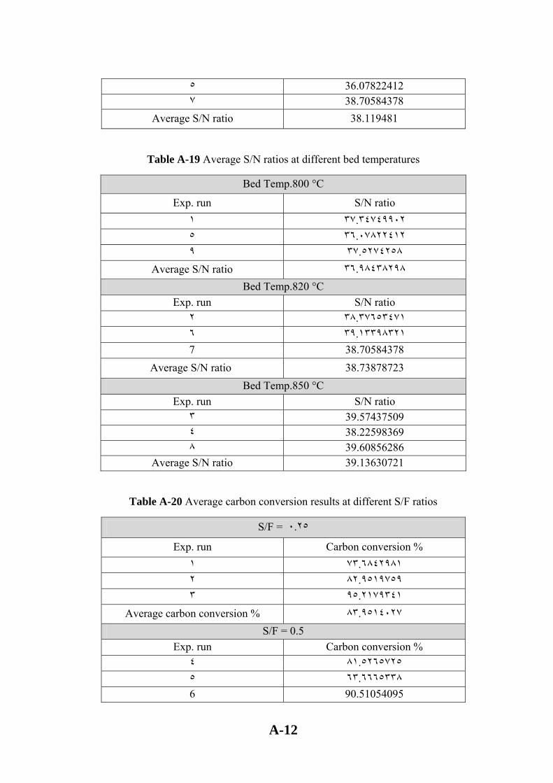
A-12
٥ 36.07822412 ٧ 38.70584378
Average S/N ratio 38.119481
Table A-19 Average S/N ratios at different bed temperatures
Bed Temp.800 °C
Exp. run S/N ratio ٣٧.٣٤٧٤٩٩٠٢ ١ ٣٦.٠٧٨٢٢٤١٢ ٥ ٣٧.٥٢٧٤٢٥٨ ٩
Average S/N ratio ٣٦.٩٨٤٣٨٢٩٨ Bed Temp.820 °C
Exp. run S/N ratio ٣٨.٣٧٦٥٣٤٧١ ٢ ٣٩.١٣٣٩٨٣٢١ ٦ 7 38.70584378
Average S/N ratio 38.73878723 Bed Temp.850 °C
Exp. run S/N ratio ٣ 39.57437509 ٤ 38.22598369 ٨ 39.60856286
Average S/N ratio 39.13630721
Table A-20 Average carbon conversion results at different S/F ratios
S/F = ٠.٢٥
Exp. run Carbon conversion % ٧٣.٦٨٤٢٩٨١ ١ ٨٢.٩٥١٩٧٥٩ ٢ ٩٥.٢١٧٩٣٤١ ٣
Average carbon conversion % ٨٣.٩٥١٤٠٢٧ S/F = 0.5
Exp. run Carbon conversion % ٨١.٥٢٦٥٧٢٥ ٤ ٦٣.٦٦٦٥٣٣٨ ٥ 6 90.51054095
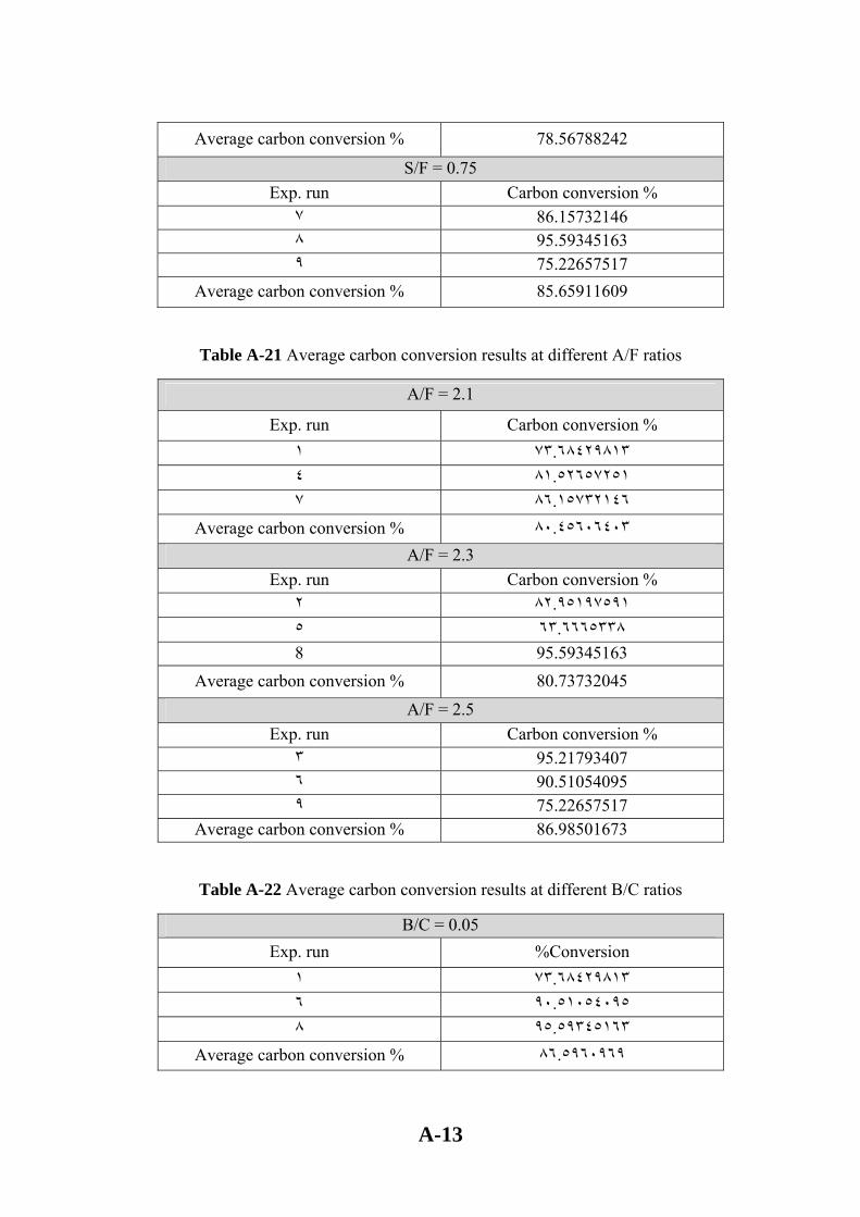
A-13
Average carbon conversion % 78.56788242
S/F = 0.75 Exp. run Carbon conversion %
٧ 86.15732146 ٨ 95.59345163 ٩ 75.22657517
Average carbon conversion % 85.65911609
Table A-21 Average carbon conversion results at different A/F ratios
A/F = 2.1
Exp. run Carbon conversion % ٧٣.٦٨٤٢٩٨١٣ ١ ٨١.٥٢٦٥٧٢٥١ ٤ ٨٦.١٥٧٣٢١٤٦ ٧
Average carbon conversion % ٨٠.٤٥٦٠٦٤٠٣ A/F = 2.3
Exp. run Carbon conversion % ٨٢.٩٥١٩٧٥٩١ ٢ ٦٣.٦٦٦٥٣٣٨ ٥ 8 95.59345163
Average carbon conversion % 80.73732045 A/F = 2.5
Exp. run Carbon conversion % ٣ 95.21793407 ٦ 90.51054095 ٩ 75.22657517
Average carbon conversion % 86.98501673
Table A-22 Average carbon conversion results at different B/C ratios
B/C = 0.05 Exp. run Conversion%
٧٣.٦٨٤٢٩٨١٣ ١ ٩٠.٥١٠٥٤٠٩٥ ٦ ٩٥.٥٩٣٤٥١٦٣ ٨
Average carbon conversion % ٨٦.٥٩٦٠٩٦٩

A-14
B/C = 0.11 Exp. run Conversion%
٨٢.٩٥١٩٧٥٩١ ٢ ٨١.٥٢٦٥٧٢٥١ ٤ 9 75.22657517
Average carbon conversion % 79.90170786 B/C = 0.25
Exp. run Conversion% ٣ 95.21793407 ٥ 63.6665338 ٧ 86.15732146
Average carbon conversion % 81.68059644
Table A-23 Average carbon conversion results at different bed temperatures
Bed Temp.800 °C Exp. run Conversion%
٧٣.٦٨٤٢٩٨١٣ ١ ٦٣.٦٦٦٥٣٣٨ ٥ ٧٥.٢٢٦٥٧٥١٧ ٩
Average carbon conversion % ٧٠.٨٥٩١٣٥٧ Bed Temp.820 °C
Exp. run Conversion% ٨٢.٩٥١٩٧٥٩١ ٢ ٩٠.٥١٠٥٤٠٩٥ ٦ 7 86.15732146
Average carbon conversion % 86.53994611 Bed Temp.850 °C
Exp. run Conversion% ٣ 95.21793407 ٤ 81.52657251 ٨ 95.59345163
Average carbon conversion % 90.7793194
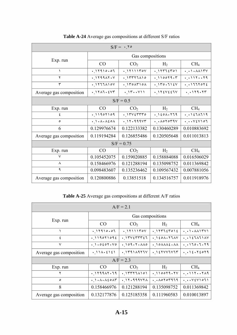
A-15
Table A-24 Average gas compositions at different S/F ratios
S/F = ٠.٢٥
Exp. run Gas compositions
CO CO2 H2 CH4 ٠.٠١٠٨٨١٣٧ ٠.١٢٣٦٤٣٥١ ٠.١٢١١١٣٥٧ ٠.١٢٩١٥٠٥٦ ١ ٠.٠١١٢٠٠٢٩ ٠.١١٥٥٢٩٠٣ ٠.١٣٣٢٦٨١٥ ٠.١٢٩٩٨٢٠٧ ٢ ٠.٠١٦٦٢٥٢٤ ٠.١٣٥٠٦١٤٧ ٠.١٣٥٨٣١٥٨ ٠.١٢٦٦٨١٥٧ ٣
Average gas composition ٠.٠١٢٩٠٢٣ ٠.١٢٤٧٤٤٦٧ ٠.١٣٠٠٧١١ ٠.١٢٨٦٠٤٧٣
S/F = 0.5 Exp. run CO CO2 H2 CH4
٠.٠١٤٦٨٦١٩ ٠.١٤٥٨٠٢٦٩ ٠.١٣٧٤٣٣٣٥ ٠.١١٩٥٢١٥٩ ٤ ٠.٠٠٧٤٧١٥٦ ٠.٠٨٥٢٥٣٩٧ ٠.١٢٠٩٩٩٧٣ ٠.١٠٨٠٨٤٥٨ ٥ 6 0.129976674 0.122133382 0.130460289 0.010883692
Average gas composition 0.119194284 0.126855486 0.120505648 0.011013813 S/F = 0.75
Exp. run CO CO2 H2 CH4 ٧ 0.105452075 0.159020885 0.158884088 0.016506029 ٨ 0.158466976 0.121288194 0.135098752 0.011369842 ٩ 0.098483607 0.135236462 0.109567432 0.007881056
Average gas composition 0.120800886 0.13851518 0.134516757 0.011918976
Table A-25 Average gas compositions at different A/F ratios
A/F = 2.1
Exp. run Gas compositions
CO CO2 H2 CH4 ٠.١٢٣٦٤٣٥١٤ ٠.١٢١١١٣٥٧ ٠.١٢٩١٥٠٥٦ ١ ٠.٠١٠٨٨١٣٧١٠.١١٩٥٢١٥٩٤ ٤ ٠.١٣٧٤٣٣٣٤٦ ٠.١٤٥٨٠٢٦٨٧ ٠.٠١٤٦٨٦١٨٧٠.١٠٥٤٥٢٠٧٥ ٧ ٠.١٥٩٠٢٠٨٨٥ ٠.١٥٨٨٨٤٠٨٨ ٠.٠١٦٥٠٦٠٢٩
Average gas composition ٠.١٣٩١٨٩٢٦٧ ٠.١١٨٠٤١٤١ ٠.١٤٢٧٧٦٧٦٣ ٠.٠١٤٠٢٤٥٢٩A/F = 2.3
Exp. run CO CO2 H2 CH4 ٠.١٢٩٩٨٢٠٦٩ ٢ ٠.١٣٣٢٦٨١٥١ ٠.١١٥٥٢٩٠٢٧ ٠.٠١١٢٠٠٢٨٩٠.١٠٨٠٨٤٥٨٣ ٥ ٠.١٢٠٩٩٩٧٢٨ ٠.٠٨٥٢٥٣٩٦٩ ٠.٠٠٧٤٧١٥٦١8 0.158466976 0.121288194 0.135098752 0.011369842
Average gas composition 0.132177876 0.125185358 0.111960583 0.010013897

A-16
A/F = 2.5 Exp. run CO CO2 H2 CH4
٣ 0.126681573 0.135831579 0.13506147 0.016625237 ٦ 0.129976674 0.122133382 0.130460289 0.010883692 ٩ 0.098483607 0.135236462 0.109567432 0.007881056
Average gas composition 0.118380618 0.131067141 0.12502973 0.011796662
Table A-26 Average gas compositions at different B/C ratios
B/C = 0.05
Exp. run Gas compositions
CO CO2 H2 CH4
٠.١٢٣٦٤٣٥١٤ ٠.١٢١١١٣٥٧ ٠.١٢٩١٥٠٥٦ ١٠.٠١٠٨٨١٣٧
١
٠.١٢٩٩٧٦٦٧٤ ٦ ٠.١٢٢١٣٣٣٨٢ ٠.١٣٠٤٦٠٢٨٩٠.٠١٠٨٨٣٦٩
٢
٠.١٥٨٤٦٦٩٧٦ ٨ ٠.١٢١٢٨٨١٩٤ ٠.١٣٥٠٩٨٧٥٢٠.٠١١٣٦٩٨٤
٢
Average gas composition ٠.١٢١٥١١٧١٥ ٠.١٣٩١٩٨٠٧ ٠.١٢٩٧٣٤١٨٥٠.٠١١٠٤٤٩٦
٨ B/C = 0.11
Exp. run CO CO2 H2 CH4
٠.١٢٩٩٨٢٠٦٩ ٢ ٠.١٣٣٢٦٨١٥١ ٠.١١٥٥٢٩٠٢٧٠.٠١١٢٠٠٢٨
٩
٠.١١٩٥٢١٥٩٤ ٤ ٠.١٣٧٤٣٣٣٤٦ ٠.١٤٥٨٠٢٦٨٧٠.٠١٤٦٨٦١٨
٧ 9 0.098483607 0.135236462 0.109567432 0.007881056
Average gas composition 0.115995757 0.135312653 0.123633049 0.011255844
B/C = 0.25 Exp. run CO CO2 H2 CH4
٣ 0.126681573 0.135831579 0.13506147 0.016625237 ٥ 0.108084583 0.120999728 0.085253969 0.007471561 ٧ 0.105452075 0.159020885 0.158884088 0.016506029
Average gas composition 0.113406077 0.138617397 0.126399842 0.013534276
Table A-27 Average gas compositions at different bed temperatures
Bed Temp.800 °C

A-17
Exp. run Gas compositions
CO CO2 H2 CH4
٠.١٢٣٦٤٣٥١٤ ٠.١٢١١١٣٥٧ ٠.١٢٩١٥٠٥٦ ١٠.٠١٠٨٨١٣٧
١
٠.١٠٨٠٨٤٥٨٣ ٥ ٠.١٢٠٩٩٩٧٢٨ ٠.٠٨٥٢٥٣٩٦٩٠.٠٠٧٤٧١٥٦
١
٠.٠٩٨٤٨٣٦٠٧ ٩ ٠.١٣٥٢٣٦٤٦٢ ٠.١٠٩٥٦٧٤٣٢٠.٠٠٧٨٨١٠٥
٦
Average gas composition ٠.١٢٥٧٨٣٢٥٣ ٠.١١١٩٠٦٢٥ ٠.١٠٦١٥٤٩٧٢٠.٠٠٨٧٤٤٦٦
٣ Bed Temp.820 °C
Exp. run CO CO2 H2 CH4
٠.١٢٩٩٨٢٠٦٩ ٢ ٠.١٣٣٢٦٨١٥١ ٠.١١٥٥٢٩٠٢٧٠.٠١١٢٠٠٢٨
٩
٠.١٢٩٩٧٦٦٧٤ ٦ ٠.١٢٢١٣٣٣٨٢ ٠.١٣٠٤٦٠٢٨٩٠.٠١٠٨٨٣٦٩
٢ 7 0.105452075 0.159020885 0.158884088 0.016506029
Average gas composition 0.121803606 0.138140806 0.134957801 0.012863336 Bed Temp.850 °C
Exp. run CO CO2 H2 CH4 ٣ 0.126681573 0.135831579 0.13506147 0.016625237 ٤ 0.119521594 0.137433346 0.145802687 0.014686187 ٨ 0.158466976 0.121288194 0.135098752 0.011369842
Average gas composition 0.134890048 0.131517706 0.138654303 0.014227089
Table A-28 Experimental results for the best coal-grape seeds experiment with A/F = 2.5, S/F ratio= 0.75, B/C =0.05, and bed Temperature = 850 °C
H2/CO ratio = 1.57, Carbon conversion = 96.1 %
Components Average molar composition
C2H2 0.0021786
CO2 0.1184116
C2H4 0.0009147
C2H6 0.0009438
H2S 1.203E-05
COS 0.0003763
C3H6 0.0007018

A-18
C3H8 0.0001457
H2 0.1975575
O2 0.0147256
N2 0.5167189
CH4 0.0102136
CO 0.1257861
Total 0.9886862
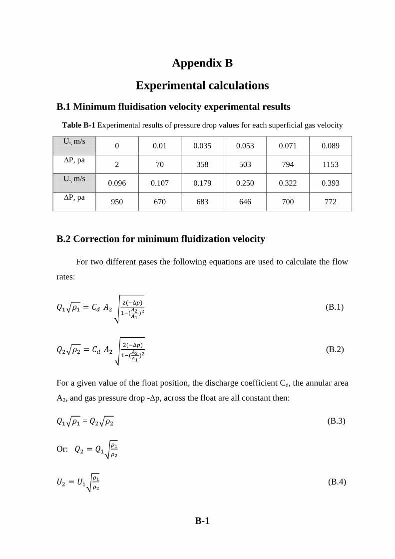
B-1
Appendix B
Experimental calculations
B.1 Minimum fluidisation velocity experimental results
Table B-1 Experimental results of pressure drop values for each superficial gas velocity
U◦, m/s
0 0.01 0.035 0.053 0.071 0.089
∆P, pa
2 70 358 503 794 1153
U◦, m/s
0.096 0.107 0.179 0.250 0.322 0.393
∆P, pa
950 670 683 646 700 772
B.2 Correction for minimum fluidization velocity
For two different gases the following equations are used to calculate the flow
rates:
√ √
(B.1)
√ √
(B.2)
For a given value of the float position, the discharge coefficient Cd, the annular area
A2, and gas pressure drop -∆p, across the float are all constant then:
√ = √ (B.3)
Or: √
√
(B.4)

B-2
Equation B.4 is used to correct the flow rate under different gases and
temperatures (Ammar, 2009).
From figure 5-1 the velocity at minimum fluidization is 0.09 m/s at 25 o
C, equation
B.4 can be used to find the value of Umf at 400 oC.
(B.5)
⁄ At 25 oC
⁄ At 400 oC
√
At 400 oC

B-3
B.3 Steam calibration results
Table B-2 Calibration data of water flow rate and mass flow rate
Reading
(L/min) 0.07 0.08 0.1 0.115 0.13 0.15 0.16 0.18 0.2
Mass flow
rate (g/h) 78 189 426 516 692 822.9 1047 1164 1357
Figure B-1 Relation between the mass flow rate of the water and rotameter readings
B.4 Feeding velocity of the fuel
Table B-3 Experimental results for the feed settling velocity experiment
Feed settling 1 2 3 4 5 6
Feed rate (g/h) 466.2 795 1137 1470 1700.4 2103
0
0.05
0.1
0.15
0.2
0.25
0 200 400 600 800 1000 1200 1400 1600
Rota
met
er r
eadin
g, L
/min
Flow rate (g/hr)

B-4
Figure B-2 Relation between feed settler velocity and the weight of fuel
B.5 Algae salt content calculation
Table B-4 Experimental results for the volatile and non-volatile in the algae
Sa
mp
le
Crucible
weight,
g
mass of
crucible +
algae before
burning, g
Mass of
algae
(dry),g
mass of
crucible +
algae after
burning, g
Mass
of ash,
g
Non volatile Volatile
1 23.4018 25.7725 2.3707 24.3846 0.9828 0.4145611 0.5854389
2 27.4798 30.3689 2.8891 28.6698 1.19 0.411892977 0.588107
3 26.4015 28.9327 2.5312 27.4433 1.0418 0.411583439 0.5884166
4 22.3683 24.5571 2.1888 23.3006 0.9323 0.425941155 0.5740588
Non volatile (average) = 0.415995
Conductance readings (mS) = 0.457
Concentration of sodium chloride = 221.3759 mg/L
(http://www.scribd.com/doc/2751385/Conductivity-Measurement)
Mass of ash = Weight of crucible with algae after burning – Weight of crucible (B.6)
0
500
1000
1500
2000
2500
0 1 2 3 4 5 6 7
fuel
wei
gh
t,g/h
feed settling velosity

B-5
Mass of ash (average) = 1.036725 g
(B.7)
(B.8)
= 0.599
(B.9)
(B.10)
Weight of leached algae = 0.93 g
(B.11)
(B.12)
The salt content in algae was calculated before leaching with the same previous
procedure and it was 42.7 %.

C-1
Appendix C
Kinetic rate expressions and fuel compositional
information
C.1 Kinetic rate expression and kinetic constants for gasification
reactions
Table C-1 Gasification reaction rates expressions (Mendes et al., 2008)
No. Reaction Kinetic rate expression and kinetic
constants, mol/m3.s
Reference
1
( )
( )
(
)
Saito et
al., (1983)
2
(
)
Tenser,
(1960)
3
(
)
Biba et
al., (1978)
4
(
)
(
)
(
)
Biba et
al., (1978)
5
(
)
(
)
Matsui et
al., (1985)
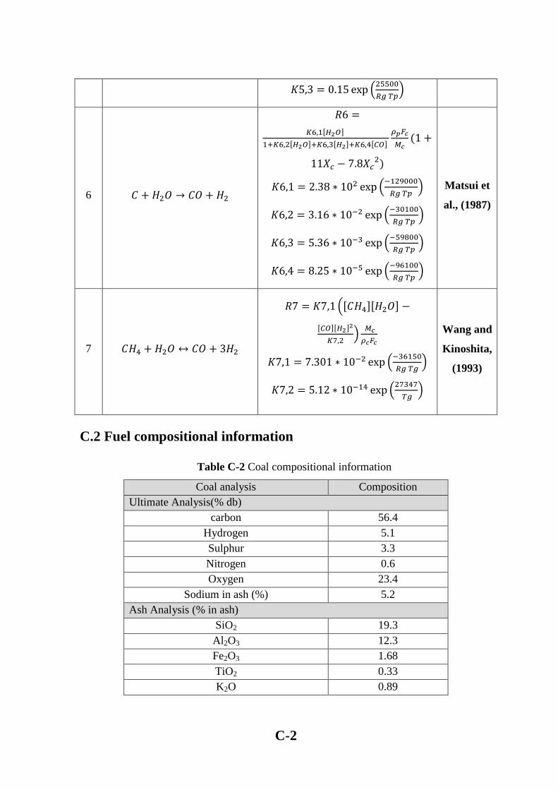
C-2
(
)
6
(
)
(
)
(
)
(
)
(
)
Matsui et
al., (1987)
7
(
)
(
)
(
)
Wang and
Kinoshita,
(1993)
C.2 Fuel compositional information
Table C-2 Coal compositional information
Coal analysis Composition
Ultimate Analysis(% db)
carbon 56.4
Hydrogen 5.1
Sulphur 3.3
Nitrogen 0.6
Oxygen 23.4
Sodium in ash (%) 5.2
Ash Analysis (% in ash)
SiO2 19.3
Al2O3 12.3
Fe2O3 1.68
TiO2 0.33
K2O 0.89
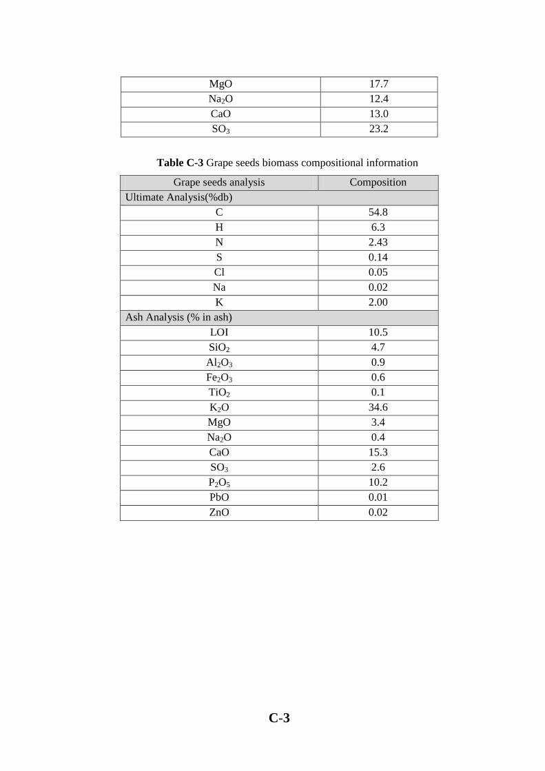
C-3
MgO 17.7
Na2O 12.4
CaO 13.0
SO3 23.2
Table C-3 Grape seeds biomass compositional information
Grape seeds analysis Composition
Ultimate Analysis(%db)
C 54.8
H 6.3
N 2.43
S 0.14
Cl 0.05
Na 0.02
K 2.00
Ash Analysis (% in ash)
LOI 10.5
SiO2 4.7
Al2O3 0.9
Fe2O3 0.6
TiO2 0.1
K2O 34.6
MgO 3.4
Na2O 0.4
CaO 15.3
SO3 2.6
P2O5 10.2
PbO 0.01
ZnO 0.02

D-1
Appendix D
Theoretical calculations
D.1 Spouting diameter (Ds)
The diameter of the spout can be calculated from Hook et al., (1992) correlation:
(
( )( ) )
(D.1)
Where:
(D.2)
is the velocity of the gas at injection point and can be calculated from:
(D.3)
(D.4)
(D.5)
(D.6)
(
)
(D.7)

D-2
Mc=0.19
(D.8)
(D.9)
wt. Coal = (1.6*4.5) = 7.2 kg
wt. Sand = 0.2 kg
*
+
D.2 Spouting velocity (us)
(D.10)
D.3 Bed porosity (ɛs)
The spout voidage is assumed to decrease linearly with z, so it will be a
variable and can be calculated at each axial distance point from the following
equation (Smith et al., 1981):

D-3
(D.11)
z represents the axial distance from the gas inlet, and H is the height of the bed
inside the gasifier and it can be calculated using Grbavcic, et al., (1976) correlation:
( (
)
) (D.12)
ums represents the velocity of the gas – phase at minimum spouting conditions
and can be calculated using Wu, et al., (1987) correlation:
*
+
*
+
*
+
[( )
]
√ (D.13)
umf is the velocity of the gas – phase at minimum fluidization conditions and
can be calculated from Littman et al., (1981) correlation:
( )
[{
( ) }
] (D.14)
Where:
The maximum spoutable height Hm can be calculated from Wu et al., (1987)
correlation:
[
] *
+
*
+ [√ ]
(D.15)
Where:
*
+
*
+ [√ ]

D-4
[
]
*
+
*
+
*
+
√
[{
}
]
The bed height H can be calculated from equation (D.12):
So, the bed porosity will calculated from:
(D.16)
D.4 Annulus gas velocity
The superficial annular gas velocity is taken from the theories of Mamuro
and Hattori, (1968) and Grbavcic et al., (1976).
[ (
)
]
[ (
)
] (D.17)
Table D-1 shows the values of bed porosity at the spout and the velocities of
the gas phase at the annulus region.

D-5
Table D-1 Values of bed porosity at the spout, and gas annulus velocities ua
z,m 0 0.013 0.026 0.039 0.052
ɛs 1 0.9954386 0.99087719 0.98631579 0.98175439
ua,m/s 0 0.00014571 0.0011657 0.00393425 0.00932564
z,m 0.065 0.078 0.091 0.104 0.117
ɛs 0.97719298 0.97263158 0.96807018 0.96350877 0.95894737
ua,m/s 0.01821414 0.03147403 0.0499796 0.07460511 0.10622486
z,m 0.13 0.143 0.156 0.169 0.182
ɛs 0.95438596 0.94982456 0.94526316 0.94070175 0.93614035
ua,m/s 0.14571311 0.19394415 0.25179225 0.3201317 0.39983677
z,m 0.195 0.208 0.221 0.234 0.247
ɛs 0.93157895 0.92701754 0.92245614 0.91789474 0.91333333
ua,m/s 0.49178174 0.59684089 0.7158885 0.84979884 0.99944621
z,m 0.26 0.273 0.286 0.299 0.312
ɛs 0.90877193 0.90421053 0.89964912 0.89508772 0.89052632
ua,m/s 1.16570486 1.34944909 1.55155317 1.77289138 2.014338
z,m 0.325 0.338 0.351 0.364 0.377
ɛs 0.88596491 0.88140351 0.87684211 0.8722807 0.8677193
ua,m/s 2.27676731 2.56105358 2.8680711 3.19869414 3.55379698
z,m 0.39 0.403 0.416 0.429 0.442
ɛs 0.86315789 0.85859649 0.85403509 0.84947368 0.84491228
ua,m/s 3.93425391 4.34093919 4.77472711 5.23649195 5.72710799
z,m 0.455 0.468 0.481 0.494 0.507
ɛs 0.84035088 0.83578947 0.83122807 0.82666667 0.82210526
ua,m/s 6.24744949 6.79839076 7.38080605 7.99556965 8.64355584
z,m 0.52 0.533 0.546 0.559 0.572
ɛs 0.81754386 0.81298246 0.80842105 0.80385965 0.79929825
ua,m/s 9.3256389 10.0426931 10.7955927 11.5852121 12.4124254

D-6
D.5 Boundary layer thickness
The mass transfer coefficient around a spherical pellet can be described by
Frӧssling correlation (Fogler, 1999).
(D.18)
Where:
(D.19)
(D.20)
(D.21)
The thickness of boundary layer can be calculated using:
(D.22)
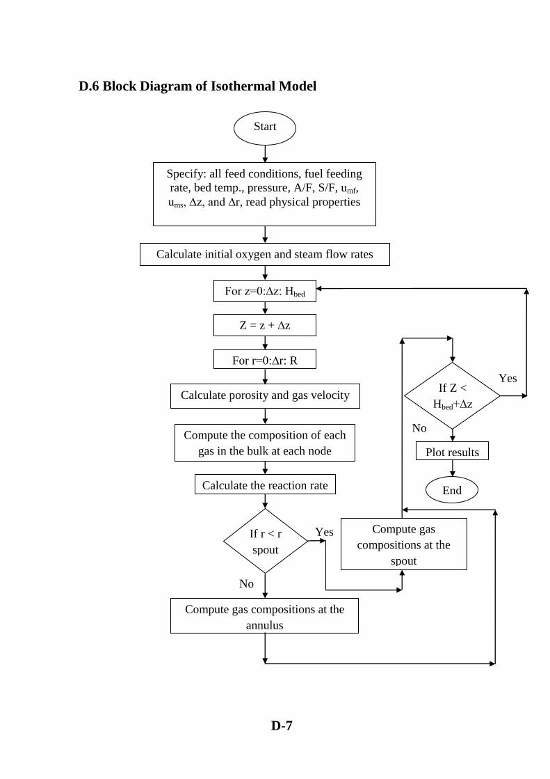
D-7
D.6 Block Diagram of Isothermal Model
Yes
Start
Specify: all feed conditions, fuel feeding
rate, bed temp., pressure, A/F, S/F, umf,
ums, ∆z, and ∆r, read physical properties
Calculate initial oxygen and steam flow rates
Calculate porosity and gas velocity
For z=0:∆z: Hbed
For r=0:∆r: R
Compute the composition of each
gas in the bulk at each node
Calculate the reaction rate
Compute gas compositions at the
annulus
If r < r
spout
Yes Compute gas
compositions at the
spout
No
Plot results
End
If Z <
Hbed+∆z
No
Z = z + ∆z

D-8
D.7 Concentration profile of gases at the spout and annulus
program
%modelling of spouted bed reactor%
%spout region%
%program to estimate the concentration of the gas with the bed height
%concentration profile of the gas - phase at the spout region
clc
clear
%Diffusivity of gases at 805C in m2/s
DiCH4=(1.1*((850+273.15)/(500+273.15))^1.75)*10^-5;
DiH2=(0.611*((850+273.15)/(273.15))^1.75)*10^-5;
DiCO=(0.185*((850+273.15)/(273.15))^1.75)*10^-5;
DiCO2=(0.138*((850+273.15)/(273.15))^1.75)*10^-5;
DiH2O=(0.220*((850+273.15)/(273.15))^1.75)*10^-5;
%Diffusivity of oxygen in air at 805C in m2/s
Di=0.73E-5;
%average diameter of coal particles, m
dp=2.175E-3;
% the axial distance from the gas inlet to the free board above the bed
z=0:0.013:0.585;
i=1:1:307;
% voidage (v) in the gasifier is the porosity
for z=0:0.013:0.585;
%height of the bed is 0.57m
H=0.57;
v=1-(0.2*z/H);
% voidage=1-v=V
V=1-v;
dz=0.013;
a=(Di*v)/dz^2;
% uz is the velocity of gas - phase at the spout in m/s
uz=0.46;
e=uz*v/dz;
dr=6.4167E-3;
h=(Di*v)/dr^2;
% R is the porosity when i=i-1
% E is the porosity when i=i+1
R=v+0.0045;
E=v-0.0046;
c=(E+v)/dz;
d=[E-2*v+R]/dz^2;
for r=0.0001:0.00641:0.019245;
g=(Di*v)/(r*dr^2);
end
b=(2*Di)/dz;
% RO2, Rair are the flow rate of oxygen and air respectively,m^3/h
RO2=0.44016;
Rair=2.1;
C1=RO2/ Rair;
D-9
%C1=Cb1 at the gasifier entrance
Cb1=C1;
%%%OXYGEN%%%
Ca1= C1*[2*a+c*b-d*Di-e+2*h+g]-[a*Cb1-c*uz+h*Cb1]/[a+c*b-e+h+g];
Ci=(((a*Ca1)+(a*Cb1)+(c*b*Ca1)-(e*Ca1)-
(c*uz)+(h*Ca1)+(h*Cb1)+(g*Ca1)/[(2*a)+(c*b)-(d*Di)-e+(2*h)+(g)]);
% Ca=C(i+1)which is the concentration of the gas phase for the node i+1
%Cb=C(i-1)which is the concentration of the gas phase for the node i-1
% C is the concentration of gas phase in the bulk at node i, spout region
Cb=Ci*[(2*a)+(c*b)-(d*Di)-e+(2*h)+g]-[(a*Ca1)+(c*b*Ca1)-(e*Ca1)-
(c*uz)+(h*Ca1)+(g*Ca1)]/[a+h];
Ca= Ci*[2*a+c*b-d*Di-e+2*h+g]-[a*Cb-c*uz+h*Cb]/[a+c*b-e+h+g];
C=(((a*Ca)+(a*Cb)+(c*b*Ca)-(e*Ca)-
(c*uz)+(h*Ca)+(h*Cb)+(g*Ca)/[(2*a)+(c*b)-(d*Di)-e+(2*h)+(g)])/(Fr+Ar));
%dr is the distance between each two nodes from the centre to the wall of
the gasifier
dr=6.41666667E-3;
A1=(Di.*v)/dr^2;
A2=(2*Di.*v)/(r*dr);
%Mc is the molar mass of carbon (kg.mol^-1)
Mc=12;
Rg=8.314;
Tg=(850+273.15);
G=((12/dp*Mc)*11.34*10^3)*exp(-711600/(Rg*Tg));
L=(0.5*8.83)*exp(-99800/(Rg*Tg));
% equation of the gas - phase concentration on the solid surface
% CO2s is the concentration of O2 at the solid surface on the spout
% region
CO2s=((A2*(Ca-C))-(A1*(Ca-2*C+Cb)))/V*(G+L);
aCH4=(DiCH4*v)/dz^2;
% uz is the velocity of gas - phase at the spout in m/s
uz=0.46;
e=uz*v/dz;
dr=6.4167E-3;
%%% Methane %%%
hCH4=(DiCH4*v)/dr^2;
for r=0.0001:0.00641:0.019245;
gCH4=(DiCH4*v)/(r*dr^2);
end
bCH4=(2*DiCH4)/dz;
% C1CH4 is the concentration of methane at z<0.013 m
C1CH4=0;
%Cb1CH4 is the concentration of methane at the gasifier entrance
Cb1CH4=0;
% Ca1 is the concentration of methane at node where z>=0.013 m
Ca1CH4=C1CH4*[2*aCH4+c*bCH4-d*DiCH4-e+2*hCH4+gCH4]-[aCH4*Cb1CH4-
c*uz+hCH4*Cb1CH4]/[aCH4+c*bCH4-e+hCH4+gCH4];
CiCH4=(((aCH4*Ca1CH4)+(aCH4*Cb1CH4)+(c*bCH4*Ca1CH4)-(e*Ca1CH4)-
(c*uz)+(hCH4*Ca1CH4)+(hCH4*Cb1CH4)+(gCH4*Ca1CH4)/[(2*aCH4)+(c*bCH4)-
(d*DiCH4)-e+(2*hCH4)+(gCH4)]));

D-10
CbCH4=CiCH4*[(2*aCH4)+(c*bCH4)-(d*DiCH4)-e+(2*hCH4)+gCH4]-
[(a*Ca1CH4)+(c*bCH4*Ca1CH4)-(e*Ca1CH4)-
(c*uz)+(h*Ca1CH4)+(gCH4*Ca1CH4)]/[aCH4+hCH4];
CaCH4=Ci*[2*aCH4+c*bCH4-d*DiCH4-e+2*hCH4+gCH4]-[aCH4*CbCH4-
c*uz+hCH4*CbCH4]/[aCH4+c*bCH4-e+hCH4+gCH4];
% C is the concentration of methane in the bulk
CCH4=(((aCH4*CaCH4)+(aCH4*CbCH4)+(c*bCH4*CaCH4)-(e*CaCH4)-
(c*uz)+(hCH4*CaCH4)+(hCH4*CbCH4)+(gCH4*CaCH4)/[(2*aCH4)+(c*bCH4)-
(d*DiCH4)-e+(2*hCH4)+(gCH4)]));
%%% HYDROGEN %%%
% SOME VARAIBLES DEPEND ON THE PHYSICAL PROPERTIES
aH2=(DiH2*v)/dz^2;
hH2=(DiH2*v)/dr^2;
for r=0.000001:0.00641:0.019245;
gH2=(DiH2*v)/(r*dr^2);
end
bH2=(2*DiH2)/dz;
% C1 is the concentration of hydrogen at z=0
C1H2=(0.04)/(0.04+0.36);
%Cb1 is the concentration of hydrogen at the gasifier entrance
Cb1H2=C1H2;
% Ca1 is the concentration of hydrogen at node where z>=0.013 m
Ca1H2=C1H2*[2*aH2+c*bH2-d*DiH2-e+2*hH2+gH2]-[aH2*Cb1H2-
c*uz+hH2*Cb1H2]/[aH2+c*bH2-e+hH2+gH2];
CiH2=(((aH2*Ca1H2)+(aH2*Cb1H2)+(c*bH2*Ca1H2)-(e*Ca1H2)-
(c*uz)+(hH2*Ca1H2)+(hH2*Cb1H2)+(gH2*Ca1H2)/[(2*aH2)+(c*bH2)-(d*DiH2)-
e+(2*hH2)+(gH2)]));
CbH2=CiH2*[(2*aH2)+(c*bH2)-(d*DiH2)-e+(2*hH2)+gH2]-
[(aH2*Ca1H2)+(c*bH2*Ca1H2)-(e*Ca1H2)-
(c*uz)+(hH2*Ca1H2)+(gH2*Ca1H2)]/[aH2+hH2];
CaH2=CiH2*[2*aH2+c*bH2-d*DiH2-e+2*hH2+gH2]-[aH2*CbH2-
c*uz+hH2*CbH2]/[aH2+c*bH2-e+hH2+gH2];
z=0:0.013:0.585;
% C is the concentration of hydrogen in the bulk
CH2=(((aH2*CaH2)+(aH2*CbH2)+(c*bH2*CaH2)-(e*CaH2)-
(c*uz)+(hH2*CaH2)+(hH2*CbH2)+(gH2*CaH2)/[(2*aH2)+(c*bH2)-(d*DiH2)-
e+(2*hH2)+(gH2)]));
%%% CARBON MONOXIDE %%%
aCO=(DiCO*v)/dz^2;
hCO=(DiCO*v)/dr^2;
for r=0.0001:0.00641:0.019245;
gCO=(DiCO*v)/(r*dr^2);
end
bCO=(2*DiCO)/dz;
% C1 is the concentration of carbon monoxide at z=0
C1CO=0;
%Cb1 is the concentration of carbon monoxide at the gasifier entrance
Cb1CO=0;
% Ca1 is the concentration of carbon monoxide at node where z>=0.013 m
Ca1CO=C1CO*[2*aCO+c*bCO-d*DiCO-e+2*hCO+gCO]-[aCO*Cb1CO-
c*uz+hCO*Cb1CO]/[aCO+c*bCO-e+hCO+gCO];

D-11
CiCO=(((aCO*Ca1CO)+(aCO*Cb1CO)+(c*bCO*Ca1CO)-(e*Ca1CO)-
(c*uz)+(hCO*Ca1CO)+(hCO*Cb1CO)+(gCO*Ca1CO)/[(2*aCO)+(c*bCO)-(d*DiCO)-
e+(2*hCO)+(gCO)]));
CbCO=CiCO*[(2*aCO)+(c*bCO)-(d*DiCO)-e+(2*hCO)+gCO]-
[(aCO*Ca1CO)+(c*bCO*Ca1CO)-(e*Ca1CO)-
(c*uz)+(hCO*Ca1CO)+(gCO*Ca1CO)]/[aCO+hCO];
CaCO=CiCO*[2*aCO+c*bCO-d*DiCO-e+2*hCO+gCO]-[aCO*CbCO-
c*uz+hCO*CbCO]/[aCO+c*bCO-e+hCO+gCO];
% C is the concentration of carbon monoxide in the bulk
CCO=(((aCO*CaCO)+(aCO*CbCO)+(c*bCO*CaCO)-(e*CaCO)-
(c*uz)+(hCO*CaCO)+(hCO*CbCO)+(gCO*CaCO)/[(2*aCO)+(c*bCO)-(d*DiCO)-
e+(2*hCO)+(gCO)]));
%%% CARBON DIOXIDE %%%
aCO2=(DiCO2*v)/dz^2;
hCO2=(DiCO2*v)/dr^2;
for r=0.0001:0.00641:0.019245;
gCO2=(DiCO2*v)/(r*dr^2);
end
bCO2=(2*DiCO2)/dz;
%C1 is the concentration of carbon dioxide at z=0
C1CO2=0;
%Cb1 is the concentration of carbon dioxide at the gasifier entrance
Cb1CO2=0;
% Ca1 is the concentration of carbon dioxide at node where z>=0.013 m
Ca1CO2=C1CO2*[2*aCO2+c*bCO2-d*DiCO2-e+2*hCO2+gCO2]-[aCO2*Cb1CO2-
c*uz+hCO2*Cb1CO2]/[aCO2+c*bCO2-e+hCO2+gCO2];
CiCO2=(((aCO2*Ca1CO2)+(aCO2*Cb1CO2)+(c*bCO2*Ca1CO2)-(e*Ca1CO2)-
(c*uz)+(hCO2*Ca1CO2)+(hCO2*Cb1CO2)+(gCO2*Ca1CO2)/[(2*aCO2)+(c*bCO2)-
(d*DiCO2)-e+(2*hCO2)+(gCO2)]));
CbCO2=CiCO2*[(2*aCO2)+(c*bCO2)-(d*DiCO2)-e+(2*hCO2)+gCO2]-
[(aCO2*Ca1CO2)+(c*bCO2*Ca1CO2)-(e*Ca1CO2)-
(c*uz)+(hCO2*Ca1CO2)+(gCO2*Ca1CO2)]/[aCO2+hCO2];
CaCO2=CiCO2*[2*aCO2+c*bCO2-d*DiCO2-e+2*hCO2+gCO2]-[aCO2*CbCO2-
c*uz+hCO2*CbCO2]/[aCO2+c*bCO2-e+hCO2+gCO2];
% C is the concentration of carbon dioxide in the bulk
CCO2=(((aCO2*CaCO2)+(aCO2*CbCO2)+(c*bCO2*CaCO2)-(e*CaCO2)-
(c*uz)+(hCO2*CaCO2)+(hCO2*CbCO2)+(gCO2*CaCO2)/[(2*aCO2)+(c*bCO2)-
(d*DiCO2)-e+(2*hCO2)+(gCO2)]));
%%% STEAM (H2O) %%%
% SOME VARAIBLES DEPEND ON THE PHYSICAL PROPERTIES
aH2O=(DiH2O*v)/dz^2;
hH2O=(DiH2O*v)/dr^2;
for r=0.0001:0.00641:0.019245;
gH2O=(DiH2O*v)/(r*dr^2);
end
bH2O=(2*DiH2O)/dz;
% C1 is the concentration of steam at z=0 m = Cb1
C1H2O=(0.346)/(0.346+2.575);
%Cb1 is the concentration of steam at the gasifier entrance
Cb1H2O=C1H2O;
% Ca1 is the concentration of steam at node where z>=0.013 m

D-12
Ca1H2O=C1H2O*[2*aH2O+c*bH2O-d*DiH2O-e+2*hH2O+gH2O]-[aH2O*Cb1H2O-
c*uz+hH2O*Cb1H2O]/[aH2O+c*bH2O-e+hH2O+gH2O];
CiH2O=(((aH2O*Ca1H2O)+(aH2O*Cb1H2O)+(c*bH2O*Ca1H2O)-(e*Ca1H2O)-
(c*uz)+(hH2O*Ca1H2O)+(hH2O*Cb1H2O)+(gH2O*Ca1H2O)/[(2*aH2O)+(c*bH2O)-
(d*DiH2O)-e+(2*hH2O)+(gH2O)]));
CbH2O=CiH2O*[(2*aH2O)+(c*bH2O)-(d*DiH2O)-e+(2*hH2O)+gH2O]-
[(aH2O*Ca1H2O)+(c*bH2O*Ca1H2O)-(e*Ca1H2O)-
(c*uz)+(hH2O*Ca1H2O)+(gH2O*Ca1H2O)]/[aH2O+hH2O];
CaH2O=CiH2O*[2*aH2O+c*bH2O-d*DiH2O-e+2*hH2O+gH2O]-[aH2O*CbH2O-
c*uz+hH2O*CbH2O]/[aH2O+c*bH2O-e+hH2O+gH2O];
% C is the concentration of steam in the bulk
CH2O=(((aH2O*CaH2O)+(aH2O*CbH2O)+(c*bH2O*CaH2O)-(e*CaH2O)-
(c*uz)+(hH2O*CaH2O)+(hH2O*CbH2O)+(gH2O*CaH2O)/[(2*aH2O)+(c*bH2O)-
(d*DiH2O)-e+(2*hH2O)+(gH2O)]));
%%%%%% equations for each gas component can be written%%%%%
%%%%%%% in the spout as follows %%%%%%%
%dr is the distance between each two nodes from the centre to the wall of
the gasifier
dr=6.41666667E-3;
A1=(Di.*v)/dr^2;
A2=(2*Di.*v)/(r*dr);
%Mc is the molar mass of carbon (kg.mol^-1)
Mc=12;
Rg=8.314;
Tg=(850+273.15);
%equation of the gas - phase concentration on the solid surface
G=((12/dp*Mc)*11.34*10^3)*exp(-711600/(Rg*Tg));
L=(0.5*8.83)*exp(-99800/(Rg*Tg));
%dpa is the density of the solid - phase in kg/m^3
dpa=672.28;
%Fc is the carbon fraction in coal=0.45
Fc=0.45;
%Xc is the carbon conversion
Xc=0.91;
H1=((dpa*Fc)/Mc)*(1-11*Xc-7.8*Xc^2);
H2=Mc/(dpa*Fc);
k1=2.778 *exp(-12560/(Rg*Tg));
k2=0.0265 *exp(32910/(Rg*Tg));
%Tp is the bed temperature=(850+273.15)K
Tp=(850+273.15);
k1a=11.34*10^3 *exp((-71160)/(Rg*Tp));
k2a=8.83*10^11 *exp((-99800)/(Rg*Tg));
k3a=8.83*10^11 *exp((-99800)/(Rg*Tg));
k3=4.89*10^10 *exp(-268000/(Rg*Tp));
k4=6.6*10^-2;
k5=0.15*exp(25500/(Rg*Tp));
k6=2.38*10^2 *exp((-129000)/(Rg*Tp));
k7=3.16*10^-2 *exp((-30100)/(Rg*Tp));
k8=5.36*10^-3 *exp((-59800)/(Rg*Tp));
k9=8.25*10^-5 *exp((-96100)/(Rg*Tp));

D-13
k10=7.301*10^-2 *exp((-36150)/(Rg*Tg));
k11=5.12*10^-14 *exp(27347/(Tg));
%%%%%%%%%%%GASES CONCENTRATION PROFILE IN THE SPOUT%%%%%%%%%%%%
%methane%
%CCH4s is the concentration of methane at the spout
CCH4s=(((A2*(CaCH4+CCH4))-(A1*(CaCH4-
2*CCH4+CbCH4)))+((CCO*CH2^2/k11)*H2)/k10*CH2O)*(G+L)/V;
%carbon monoxide%
%CCO is the concentration of carbon monoxide
%CCOs is the concentration of carbon monoxide at the solid - surface
BCO=(k1*CH2)+((1/k3*CCO2*H1)/(1+k4*CCO2+k5))+((1/1+k7*CH2O+k8*CH2+k9))-
H2*(CH2^2/k11);
CCOs=((A2*(CaCO-CCO))-(A1*(CaCO-2*CCO+CbCO)))+((CO2s*CCH4s)/k2)-
(k10*H2*CCH4s*CH2O)/V*BCO;
%carbon dioxide%
%CCO2 is the concentration of carbon dioxide in the spout region
%CCO2s is the concentration of carbon dioxide in the spout
CCO2s=((A2*(CaCO2-CCO2))-(A1*(CaCO2-
2*CCO2+CbCO2)))+(k2*((6/dp*Mc)*k1a*CO2s+k2a*CCOs*CO2s+k1*CCOs*CH2O))/V*k1
*CH2;
%Hydrogen%
%CH2 is the concentration of hydrogen
%CH2s is the concentration of hydrogen in the spout
CH2s=((A2*(CaH2-CH2))-(A1*(CaH2-2*CH2+CbH2)))+(-1*k1*CCOs*CH2O-
k10*CCH4s*CH2O)/((6/dp)*k3a-
k1*CCO2/k2+((H1/1+k7*CH2O+k8+k9*CCOs)/(k6*CH2O)))/V;
%Steam%
%CH2O is the concentration of steam
%CH2Os is the concentration of steam in the spout
CH2Osc=(((A2*(CaH2O-CH2O))-(A1*(CaH2O-
2*CH2O+CbH2O)))+(k1*CCO2s*CH2s/k2)+(k10*CCOs*CH2s^2*H2/k11))/V;
%%% corrected equation %%%
% methane %
CCH4sc=(((A2*(CaCH4+CCH4))-(A1*(CaCH4-
2*CCH4+CbCH4)))+((CCOs*CH2s^2/k11)*H2)/k10*CH2Osc)*(G+L)/V;
%carbon monoxide%
BCO=(k1*CH2)+((1/k3*CCO2*H1)/(1+k4*CCO2+k5))+((1/1+k7*CH2O+k8*CH2+k9))-
H2*(CH2^2/k11);
CCOsc=((A2*(CaCO-CCO))-(A1*(CaCO-2*CCOs+CbCO)))+((CO2s*CCH4sc)/k2)-
(k10*H2*CCH4sc*CH2Osc)/V*BCO;
%carbon dioxide%
CCO2sc=((A2*(CaCO2-CCO2))-(A1*(CaCO2-
2*CCO2+CbCO2)))+(k2*((6/dp*Mc)*k1a*CO2s+k2a*CCOs*CO2s+k1*CCOs*CH2Osc))/V*
k1*CH2s;
%Hydrogen%
CH2sc=((A2*(CaH2-CH2))-(A1*(CaH2-2*CH2+CbH2)))+(-1*k1*CCOs*CH2Osc-
k10*CCH4sc*CH2Osc)/((6/dp)*k3a-k1*CCO2/k2+((H1/1+k7*CH2Osc+k8+k9*CCOs)-
((k10*CCOsc^2)/k11)/(k6*CH2Osc)))/V;

D-14
% the concentration of the gas - phase on the solid surface in the
annulus region %
% ua is the velocity of the gas - phase at the annulus region, m/s
% umf is the minimum fluidization velocity of the gas - phase at the
% annulus region, m/s
% Hm is the maximum spoutable height, m
for z=0:0.013:0.585;
Hm=0.211;
umf=0.708;
ua=0.88*umf*(1-(1-(z/Hm)^3));
end
b1=(v*ua)/dz;
c1=v/dz;
h=(2*Di*v)/(dr);
hCOa=(2*DiCO*v)/(dr);
hCO2a=(2*DiCO2*v)/(dr);
hH2a=(2*DiH2*v)/(dr);
hH2Oa=(2*DiH2O*v)/(dr);
hCH4a=(2*DiCH4*v)/(dr);
% ra is the radius where the nodes lie at the annulus region
for ra=0.019245:0.00641:0.0385;
z=0:0.013:0.585;
g1=(Di*v)/(ra*dr);
g1CO=(DiCO*v)/(ra*dr);
g1CO2=(DiCO2*v)/(ra*dr);
g1H2=(DiH2*v)/(ra*dr);
g1H2O=(DiH2O*v)/(ra*dr);
g1CH4=(DiCH4*v)/(ra*dr);
end
% Cga is the concentration of the gas - phase at the annulus region
for z=0.013:0.013:0.585;
uai=0.88*umf*(1-(1-(z/Hm)^3));
end
%%%% OXYGEN %%%%
%Cba is the of the gas - phase in the annulus region at node i-1
%Cb1 is the initial concentration of the gas - phase in the annulus
region
Cba=Cb1;
%Cga is the initial concentration of the gas - phase at node i=1
Cga=C1;
Caa=(C1*[2*a-b1+2*h+g1]-a*Cba+c1*(uai-ua)-h*Cba)/a-b1+h+g1;
for z=0:0.013:0.585;
Cga=[(a*Caa)+(a*Cba)-(b1*Caa)-c1*(uai-
ua)+(h*Caa)+(h*Cba)+(g1*Caa)]/[2*a-b1+2*h+g1];
% Cba1 is the concentration of the gas - phase in the annulus region for
% the nodes lie before the node i , i.e, for i-1
Cba1=(Cga*[a-b1+2*h+g1]+a*Caa+b1*Caa+c1*(uai-ua)-h*Caa-g1*Caa)/a+h;
% Caa1 is the concentration of the gas - phase in the annulus region for
% the nodes lie before the node i , i.e, for i+1

D-15
Caa1=(Ci*[a-b1+2*h+g1]+a*Cba1+c1*(uai-ua)-h*Cba1)/a-b1+h+g1;
% Cga1 is the concentration of the gas - phase in the annulus region on
% the node i
Cga1=[[(a*Caa1)+(a*Cba1)-(b1*Caa1)-c1*(uai-
ua)+(h*Caa1)+(h*Cba1)+(g1*Caa1)]/[2*a-b1+2*h+g1]];
Ga=((12/dp*Mc)*11.34*10^3)*exp(-711600/(Rg*Tg));
La=(0.5*0.0883)*exp(-99800/(Rg*Tg));
% CO2s is the concentration of O2 at the solid surface on the annulus
% region
CO2a=((A1*(Caa1-Cga1))-(A2*(Caa1+2*Cga1+Cba1)))/V*(Ga+La);
%%%% Steam %%%%
CbaH2O=0;
CgaH2O=C1H2O;
CaaH2O=(C1H2O*[2*a-b1+2*hH2Oa+g1H2O]-a*CbaH2O+c1*(uai-ua)-
hH2Oa*CbaH2O)/a-b1+hH2Oa+g1H2O;
CgaH2O=[(a*CaaH2O)+(a*CbaH2O)-(b1*CaaH2O)-c1*(uai-
ua)+(hH2Oa*CaaH2O)+(hH2Oa*CbaH2O)+(g1H2O*CaaH2O)]/[2*a-b1+2*hH2Oa+g1H2O];
% Cba1 is the concentration of steam in the annulus region at
% node i-1
Cba1H2O=(CgaH2O*[a-b1+2*hH2Oa+g1H2O]+a*CaaH2O+b1*CaaH2O+c1*(uai-ua)-
hH2Oa*CaaH2O-g1H2O*CaaH2O)/a+hH2Oa;
% Caa1 is the concentration of steam in the annulus region at node
% i+1
Caa1H2O=(CgaH2O*[a-b1+2*hH2Oa+g1H2O]+a*Cba1H2O+c1*(uai-ua)-
hH2Oa*Cba1H2O)/a-b1+hH2Oa+g1H2O;
% Cga1 is the concentration of the gas - phase in the annulus region at
% the node i
Cga1H2O=[[(a*Caa1H2O)+(a*Cba1H2O)-(b1*Caa1H2O)-c1*(uai-
ua)+(hH2Oa*Caa1H2O)+(hH2Oa*Cba1H2O)+(g1H2O*Caa1H2O)]/[2*a-
b1+2*hH2Oa+g1H2O]];
% CCO2s is the concentration of H2O at the solid surface on the annulus
% region
CH2Oa=((A1*(Caa1H2O-Cga1H2O))-
(A2*(Caa1H2O+2*Cga1H2O+Cba1H2O)))/V*(Ga+La);
%%%% carbon dioxide %%%%
CbaCO2=0;
CgaCO2=C1CO2;
CaaCO2=(C1CO2*[2*a-b1+2*hCO2a+g1CO2]-a*CbaCO2+c1*(uai-ua)-
hCO2a*CbaCO2)/a-b1+hCO2a+g1CO2;
CgaCO2=[(a*CaaCO2)+(a*CbaCO2)-(b1*CaaCO2)-c1*(uai-
ua)+(hCO2a*CaaCO2)+(hCO2a*CbaCO2)+(g1CO2*CaaCO2)]/[2*a-b1+2*hCO2a+g1CO2];
% Cba1 is the concentration of carbon dioxide in the annulus region at
% node i-1
Cba1CO2=(CgaCO2*[a-b1+2*hCO2a+g1CO2]+a*CaaCO2+b1*CaaCO2+c1*(uai-ua)-
hCO2a*CaaCO2-g1CO2*CaaCO2)/a+hCO2a;
% Caa1 is the concentration of carbon dioxide in the annulus region at
node
% i+1
Caa1CO2=(CgaCO2*[a-b1+2*hCO2a+g1CO2]+a*Cba1CO2+c1*(uai-ua)-
hCO2a*Cba1CO2)/a-b1+hCO2a+g1CO2;
% Cga1 is the concentration of the gas - phase in the annulus region on
D-16
% the node i
Cga1CO2=[[(a*Caa1CO2)+(a*Cba1CO2)-(b1*Caa1CO2)-c1*(uai-
ua)+(hCO2a*Caa1CO2)+(hCO2a*Cba1CO2)+(g1CO2*Caa1CO2)]/[2*a-
b1+2*hCO2a+g1CO2]];
% CCO2s is the concentration of CO2 at the solid surface on the annulus
% region
CCO2a=k1*CH2*((A1*(Caa1CO2-Cga1CO2))-
(A2*(Caa1CO2+2*Cga1CO2+Cba1CO2)))/V*(k2*((6/dp*Mc)*k1a*CO2s+k2a*CCOs*CO2s
+k1*CCOs*CH2Osc));
%%%% carbon monoxide %%%%
CbaCO=0;
CgaCO=C1CO;
CaaCO=(C1CO*[2*a-b1+2*hCOa+g1CO]-a*CbaCO+c1*(uai-ua)-hCOa*CbaCO)/a-
b1+hCOa+g1CO;
CgaCO=[(a*CaaCO)+(a*CbaCO)-(b1*CaaCO)-c1*(uai-
ua)+(hCOa*CaaCO)+(hCOa*CbaCO)+(g1CO*CaaCO)]/[2*a-b1+2*hCOa+g1CO];
% Cba1 is the concentration of carbon monoxide in the annulus region at
% node i-1
Cba1CO=(CgaCO*[a-b1+2*hCOa+g1CO]+a*CaaCO+b1*CaaCO+c1*(uai-ua)-hCOa*CaaCO-
g1CO*CaaCO)/a+hCOa;
% Caa1 is the concentration of carbon monoxide in the annulus region at
node
% i+1
Caa1CO=(CgaCO*[a-b1+2*hCOa+g1CO]+a*Cba1CO+c1*(uai-ua)-hCOa*Cba1CO)/a-
b1+hCOa+g1CO;
% Cga1 is the concentration of the gas - phase in the annulus region at
% the node i
Cga1CO=[[(a*Caa1CO)+(a*Cba1CO)-(b1*Caa1CO)-c1*(uai-
ua)+(hCOa*Caa1CO)+(hCOa*Cba1CO)+(g1CO*Caa1CO)]/[2*a-b1+2*hCOa+g1CO]];
% CCO2s is the concentration of CO at the solid surface on the annulus
% region
CCOa=((A1*(Caa1CO-Cga1CO))-(A2*(Caa1CO+2*Cga1CO+Cba1CO)))/V*BCO;
%%%% Hydrogen %%%%
CbaH2=0;
CgaH2=C1H2;
CaaH2=(C1H2*[2*a-b1+2*hH2a+g1H2]-a*CbaH2+c1*(uai-ua)-hH2a*CbaH2)/a-
b1+hH2a+g1H2;
CgaH2=[(a*CaaH2)+(a*CbaH2)-(b1*CaaH2)-c1*(uai-
ua)+(hH2a*CaaH2)+(hH2a*CbaH2)+(g1H2*CaaH2)]/[2*a-b1+2*hH2a+g1H2];
% Cba1 is the concentration of hdrogen in the annulus region at
% node i-1
Cba1H2=(CgaH2*[a-b1+2*hH2a+g1H2]+a*CaaH2+b1*CaaH2+c1*(uai-ua)-hH2a*CaaH2-
g1H2*CaaH2)/a+hH2a;
% Caa1 is the concentration of hydrogen in the annulus region at node
% i+1
Caa1H2=(CgaH2*[a-b1+2*hH2a+g1H2]+a*Cba1H2+c1*(uai-ua)-hH2a*Cba1H2)/a-
b1+hH2a+g1H2;
% Cga1 is the concentration of the gas - phase in the annulus region at
% the node i
Cga1H2=[[(a*Caa1H2)+(a*Cba1H2)-(b1*Caa1H2)-c1*(uai-
ua)+(hH2a*Caa1H2)+(hH2a*Cba1H2)+(g1H2*Caa1H2)]/[2*a-b1+2*hH2a+g1H2]];

D-17
% CCO2s is the concentration of H2 at the solid surface on the annulus
% region
CH2a=((6/dp)*k3a-k1*CCO2/k2+((H1/1+k7*CH2Osc+k8+k9*CCOs)-
((k10*CCOsc^2)+((A1*(Caa1H2-Cga1H2))-(A2*(Caa1H2+2*Cga1H2+Cba1H2)))/V*(-
1*k1*CCOsc*CH2Osc-k10*CCH4sc*CH2Osc))));
end
end

E.1
coal
seco
Figu
Microgr
l gasifica
Figure E-1ondary elec
of
ure E-1b Pe
raph of
ation
1 Micrograpctronic imagf agglomera
eeks of the msection
A
SEM
SE and
ph of SEM ge for a sectate
materials incn in Fig. E-1
E-1
Appendi
analysi
BSE im
tion Fi
seco
cluded in th1
ix E
s result
ages for
igure E-1andary electr
(A) in
Tamat
he selected
ts
the aggl
Element C O Na Mg Al Si K Ca Fe
Total
Micrographronic imagen Figure E-
able E-1 Coterials in the
Fi
lomerate
Wt % 14.54 39.77
3.6 4.49 5.58
24.67 0.76 5.33 1.26 100
h of SEM e for section1
ompositionse selected sig. E-1
e from
n
s of the ection in
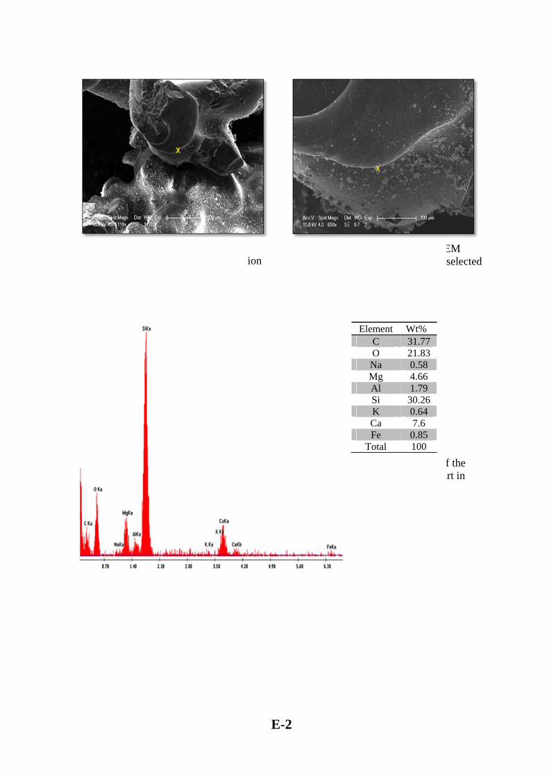
seco
Figu
Figure E-2ondary elect
of
ure E-2b Pe
2 Micrograptronic imag
f agglomerat
eeks of the mpart
ph of SEM ge for a sectite
materials inof Fig. E-2
E-2
seion
ncluded in th
Figure Eecondary ele
s
he selected
Tablmate
Element C O Na Mg Al Si K Ca Fe
Total
E-2a Microectronic imasection in Fi
le E-2 Comperials in the
Fig.
Wt% 31.77 21.83 0.58 4.66 1.79
30.26 0.64 7.6
0.85 100
ograph of SEage for the ig. E-2
mpositions ofselected paE-2
EM selected
f the art in

Figure E-backscatte
Figure Ebackscatte
-3 Micrograered image o
agglomera
E-4 Microgrered image
agglomer
aph of a SEMof a sectionate
raph of a SEof a section
rate
E-3
M n of
EM n of
Ele
M
T
ElemOF
NMASPSCKC
To
Table Ematerial
Table E-4materials
ement WO 47Na 0Mg 0Al 0Si 49S 0Cl 0K 0Ca 0
Total 1
ment WtO 49.F 0
Na 0.4Mg 0.3Al 0.5Si 48.P 0S 0Cl 0K 0.1Ca 0.3otal 10
-3 Composis in the sele
Fig. E-3
4 Compositiin the selec
Fig. E-4
Wt % 7.66
0.35 0.35 0.74 9.28
0.39 0.4
0.22 0.6 100
t % .09 0 43 39 58 .99 0 0 0 12 39 00
itions of theected part in3
tions of the cted part in
e n

E.2
alga
for t
feed
secti
Microgr
ae gasific
Figures E
the agglom
rate, 0.5
ion can be
Figure E
raph of
cation
E-5 and E-6
merate obta
S/F and a
shown in f
E-5 Microgr
SE and
6 show Mi
ained from
temperatu
front of eac
aphs of SEM
E-4
BSE im
icrographs
m the gasifi
ure of 850
ch image.
M secondar
ages for
s of SEM s
fication of
°C. Analy
ry electronic
E
the aggl
secondary
algae with
ysis results
c images of
Element O Na Mg Al Si P S Cl K Ca Fe
Total
Element O Na Mg Al Si P S Cl K Ca Fe
Total
lomerate
electronic
h 1.43 Kg/
for each s
f agglomerat
Wt % 10.86 4.97
1 58.19 3.11
0 1.89 15.17 1.61 2.24 0.97 100
Wt % 16.88 15.97 7.42 6.12 2.06 1.3
2.84 37.38 3.97 2.76 3.29 100
e from
images
/h algae
selected
te

imag
algae
selec
Figure E
Figures E
ges for the
e feed rate
cted section
Fig
E-6 Microgr
E-7 and E
agglomer
e, 0.5 S/F
n can be sh
gure E-7 Mi
aphs of SEM
E-8 shows
ate obtaine
and a tem
hown in fro
icrographs o
E-5
M secondar
Microgra
ed from th
mperature
ont of each
of SEM bac
ry electronic
aphs of SE
he gasificat
of 850 °C
h image.
ck scattered
E
Element
O Na Mg Al Si P S Cl K Ca
Total
c images of
EM back s
ion of alga
C. Analysis
d electron
lement WO Na Mg Al Si P S Cl K Ca Fe
Total
t Sec.1 Wt %
48.97 0
0.41 1.09
47.45 0
0.41 0.46 0.42 0.79 100
f agglomerat
scattered e
ae with 1.4
s results f
images
Wt % 20.95 15.48 6.71 4.68 0.93 0.92 4.47 35.08 1.19 7.79 1.81 100
Sec.2 Wt % 44.41 2.85 4.32
14.91 20.8
0 0.32 1.51 2.69 8.2 100
te
electron
43 Kg/h
for each
Sec.3 Wt % 59.5 4.13 6.85 9.93 3.32 4.23 3.89 5.82 0.95 1.38 100

zoom
algae
form
Figu
Fig
Figure
m-in for se
e feed rate
m in cluster
ure E-8a M
gure E-8 Mi
E-9 show
ection in th
, 0.5 S/F, a
rs sticking t
Micrographs
icrographs o
ws Microgr
he agglome
at 850 °C.
to each oth
of SEM bac
E-6
of SEM bac
raphs of S
erated alga
The follow
her during
ck-scattered
Fig. E-8
ck scattered
SEM back
ae results f
wing image
gasificatio
d electron im8
Elem
OF
NMASPSCKC
To
d electron
k-scattered
from the ru
es show ho
n.
mages zoom
ment SecWt
O 2.1F 0
Na 33.7Mg 0 Al 0.7Si 0.7P 0.8S 1.7Cl 58.5K 0.7Ca 0.7otal 10
images
d electron
un with 1.4
ow the salt
m-in for sect
c.1 %
Sec.2 Wt%
12 40.01 0 74 3.08 20.39 7 6.39
73 20.66 82 0.89 75 0.67 56 4.24
79 1.17 79 2.51 00 100
images
43 Kg/h
crystals
tion 1 in

for t
Kg/h
back
and
Figu
Figure E-
the bed ma
h, 0.5 S/F,
k-scattered
algae articl
ure E-9 Micthe re
-9a and b s
aterial resu
, at 850 °C
electron im
les in Figu
crographs oesults of ana
a
c
show micr
ults from g
C. Figure E
mages for t
ure E-9b).
f SEM backalysis for th
E-7
rographs of
gasification
E-9c and d
the bed ma
k-scattered he selected s
f SEM bac
n of algae
d show zo
aterial (sect
electron imsections in im
ck-scattere
with fuel
om-in mic
tion in con
ages for themages a, b,
b
d
d electron
feed rate
crographs o
ntact betwe
e bed mater c, and d.
images
of 1.43
of SEM
een sand
ial, with

Tab
E.3
leac
algae
secti
Figu
ble E-5 Com
Microgr
ching
Figure E-1
e before le
ions 1 and
ure E-10 Micomponen
Elem
ONMASPSCKCaFe
Tot
1
mpositional
raph of S
10 shows m
eaching use
2.
icrographs ont result from
ment
O a
Mg Al
i P S l
K a e tal
information
SEM ima
micrograph
ed in gasif
of SEM secm analysis i
Sec. a, Wt % 39.05 4.14 24.53 0.79 18.88
0 1.57 7.8
0.29 1.49 1.45 100
E-8
n for the sel
ages for
hs of SEM
fication wi
condary- elein sections 1
Sec. b, Wt % 5.91 30.8
0 1.04 0.55 0.51 1.96 54.15 1.01 2.85 1.21 100
4
lected sectio
the raw
secondary
ith the com
ectron image1 and 2 of ra
Sec. cWt %10.437.7
2.5627.8714.990.794.7717
2.287.254.35100
Elem
O
NMAS
CKC
To
ons in Figur
algae be
-electron im
mpositions
es and the caw algae be
c, %
SeW
3 61
7 39 0 0 0
0 1 1
ment SW
O F 0
Na Mg Al 0Si 0P 0S 0Cl 5K Ca 0otal
re E-9a, b, c
efore and
mages for
of compon
compositionefore leachin
ec. d, Wt % 6.49 15.41
0 38.96 0.17 0.65 0.72 34
0.97 1.39 1.24 100
Sec.1 Wt % 1.99 0.35 39 0
0.49 0.53 0.61 0.84
55.02 0.6
0.58 100
c, and d
d after
the raw
nents in
n of each ng.
Sec.2 Wt % 4.36 0.12
37.79 0
0.73 0.61 0.12 0.52
55.61 0
0.15 100

F
Fi
raw
secti
igure E-10
igure E-10b
Figure E
algae afte
ion.
1
a Peaks for
b Peaks for
E-11 show
er leaching
the composFig.E-10
r the compoFig.E-10 t
s microgra
g with the
E-9
sitions of rataken unde
sitions of rataken under
aphs of SE
data resul
4
aw algae ber SE detecto
aw algae ber SE detecto
EM second
ts for the
fore leachinor
fore leachinor.
dary-electro
componen
ng at section
ng at section
on images
nts in the s
n 1 in
n 2 in
for the
selected

Figuc
Figu
ure E-11 Micomponent
ure E-11a P
1
icrographs oresult from
Peaks for tha
of SEM secanalysis in
he compositafter leachin
E-10
condary- elen the selecte
tions in the ng taken un
4
ectron imaged sections o
selected secnder SE dete
es and the cof raw algae
ction in Fig.ector
Element O F
Na Mg Al Si P S Cl K Ca
Total
compositione after leach
. E-11 of raw
Wt% 45.8
0 3.01 6.38
10.21 1.41 1.91
12.26 8
1.55 9.48 100
n of each hing.
w algae
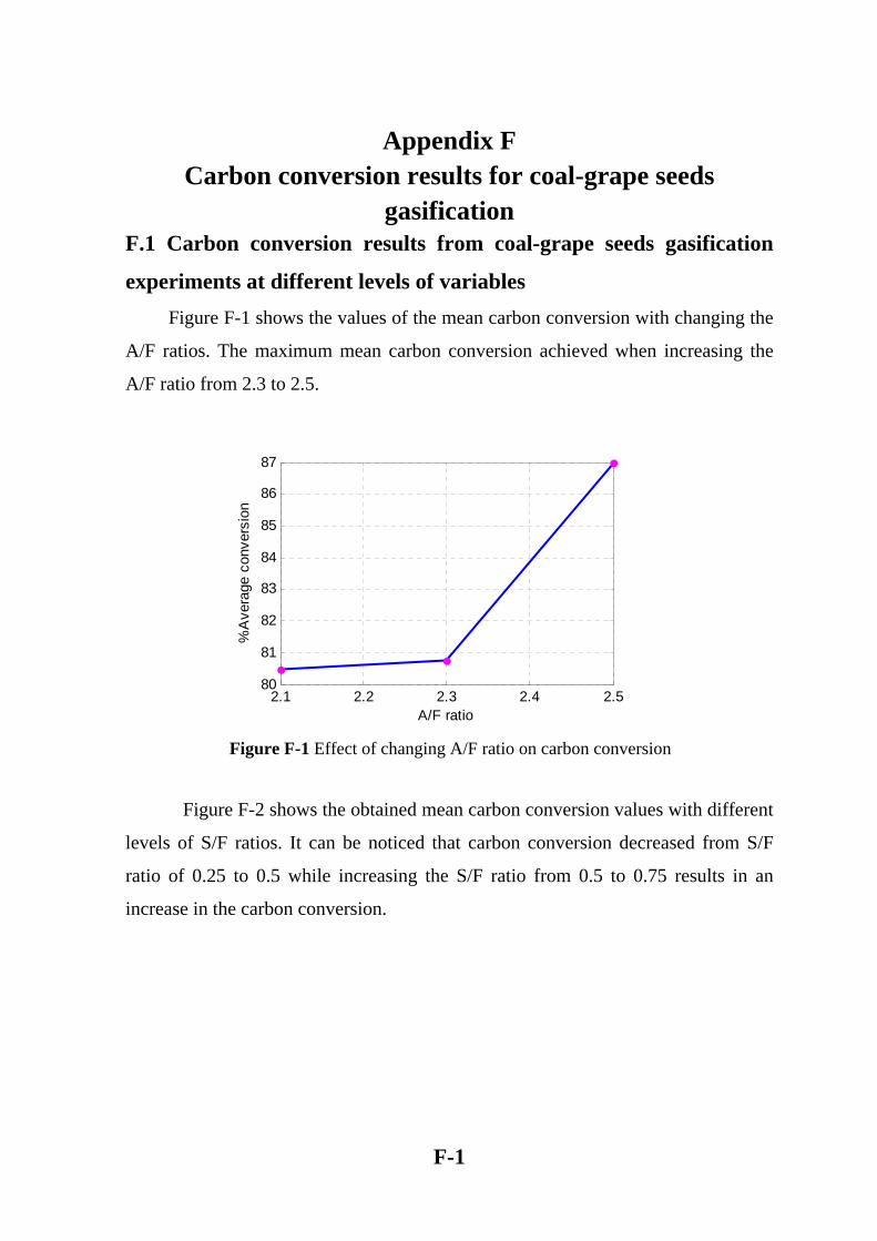
F-1
Appendix F Carbon conversion results for coal-grape seeds
gasification F.1 Carbon conversion results from coal-grape seeds gasification
experiments at different levels of variables Figure F-1 shows the values of the mean carbon conversion with changing the
A/F ratios. The maximum mean carbon conversion achieved when increasing the
A/F ratio from 2.3 to 2.5.
Figure F-2 shows the obtained mean carbon conversion values with different
levels of S/F ratios. It can be noticed that carbon conversion decreased from S/F
ratio of 0.25 to 0.5 while increasing the S/F ratio from 0.5 to 0.75 results in an
increase in the carbon conversion.
2.1 2.2 2.3 2.4 2.580
81
82
83
84
85
86
87
A/F ratio
%A
vera
ge c
onve
rsio
n
Figure F-1 Effect of changing A/F ratio on carbon conversion

F-2
Figure F-3 shows the carbon conversion results when changing the bed
temperature. The carbon conversion increased with increasing bed temperature and
the maximum conversion achieved when increasing the temperature from 820 °C to
850 °C.
0.25 0.35 0.45 0.55 0.65 0.750.7578
80
82
84
86
S/F ratio
%A
vera
ge c
onve
rsio
n
800 810 820 830 840 85070
75
80
85
90
95
Temperature,C
%A
vera
ge c
onve
rsio
n
Figure F-2 Effect of changing S/F ratio on carbon conversion
Figure F-3 Effect of changing the bed temperature on carbon conversion

F-3
Figure F-4 shows the obtained carbon conversion values at different biomass
to coal ratios. Changing the ratio of B/C from 0.05 to 0.11 decreased the carbon
conversion while increasing the B/C from 0.11 to 0.25 results in slightly increase in
the carbon conversion which concluded that changing the B/C ratio has a less effect
on the carbon conversion.
0.05 0.1 0.15 0.2 0.2578
80
82
84
86
88
B/C ratio
%A
vera
ge c
onve
rsio
n
Figure F-4 Effect of changing the B/C ratio on carbon conversion

الخلاصةرتفاع آلفة النفط الخام والحاجة المتزايدة لوقود النقل تم استخدام مواد خام قليلة الكلفة مثل الفحم وبقايا مع إ
الكتلة العضوية آمصدراقتصادي لانتاج وقود النقل أو لتوليد الطاقة الكهربائية باستعمال مفاعل الطبقة المميعة
لوقود الصلب، حيث يعتبرمفاعل الطبقة المميعة من التقنيات الراسخة بعد ربطه مع محرك الغاز لتحويل ا
ستعمال. رة الأوالكثي
بتحويل الفحم، الغاز الحيويالعمل الحالي يهتم بدراسة آليات تفاعلات التحويل إلى الغاز لإنتاج
المنطلق للتحويل الى الغاز الفحم في مفاعل الطبقة المميعة -عنبال وبذور الفحم-الطحالب، مشارك من طحالب
تحت تأثير ظروف تشغيلية مختلفة. نظريا، تم وضع موديل رياضي لحساب تراآيز الغازات الناتجة من عملية
حرارة.الالتحويل الى الغازبثبوت
ة في مفاعل الطبقة المميع غاز الحيويالطحالب الى ال - الجزء العملي يهتم بتحويل الفحم، الطحالب، والفحم
. تم دراسة تأثير تغيير داخل المفاعلوسط لنقل الحرارة وللمزج المنطلق للتحويل الى الغاز باستخدام الرمل آ
,0.5 ,0) درجة سيليزية، نسبة البخار الى الوقود (٨٥٠، ٨٢٠الظروف التشغيلية مثل درجة الحرارة (
فقد غاز الحيويبذور العنب الى ال -ل الفحم). أما في عملية تحوي2 ,1.8 ,1.6)، نسبة الهواء الى الوقود (0.75
، ٨٥٠تم اعتماد طريقة تاجوشي في تصميم التجارب لدراسة مختلف الظروف التشغيلية مثل درجة الحرارة (
، (2.5 ,2.3 ,2.1)نسبة الهواء الى الوقود ، (0.75 ,0.5 ,0.25))، نسبة البخار الى الوقود ٨٠٠,٨٢٠
.(0.25 ,0.11 ,0.05)ونسبة البايوماس الى الفحم
نقص عند زيادة درجة الحرارة في حالة آمية CO2، ترآيز غاز الحيويفي عملية تحويل الفحم الى ال
آمية زداد مع زيادة درجة الحرارة. في حالة زيادة اH2، CO ، CH4تغذية الوقود المنخفضة بينما ترآيز
درجة الحرارة.زداد بزيادة اCO2، CO، H2، CH4تغذية الوقود، ترآيز
للمادة المتفاعلة مع الرمل اضافة البخار الى الهواء المتفاعل مع الوقود الصلب أدى الى منع حدوث تكتل
. CO ونقصان في ترآيزCH4 و H2، COداخل المفاعل. زيادة نسبة البخار الى الوقود أدى الى زيادة ترآيز
أما في درجات د بزيادة نسبة الهواء الى الوقود،زداان في درجات الحرارة المنخفضة ترآيز غاز الهيدروجي
الحرارة المرتفعة زيادة نسبة الهواء الى الوقود أدت الى نقصان ترآيزغاز الهيدروجين الناتج. الظروف
نسبة البخار ، ١.٨هي: نسبة الهواء الى الوقود= غاز الحيويالتشغيلية المثلى في عملية تحويل الفحم الى ال
درجة سيليزية. في هذه الظروف تم الحصول على اعلى نسبة ٨٥٠، ودرجة الحرارة= ٠.٧٥ود=الى الوق
.H2:CO=2.197واعلى نسبة %92.9تحول للكاربون=
الطحالب المرشحة أدى الى حدوث تكسر أو -عملية التحويل للغاز لوقود الطحالب الغيرمرشحة و الفحم
وتحولها الى جزيئات صغيرة الحجم تتطاير بسهولة عند دخولها طحن لجزيئات الطحالب في وحدة التغذية
نابيب مرور الغاز الناتج.أاعل مما تسبب في حدوث انسداد في المف

اأثبتت ان درجة الحرارة هي المتغير الأآثر تأثير غاز الحيويبذور العنب الى ال -تجارب تحويل الفحم
على نسبة تحول الكاربون. اعلى نسبة تحول الكاربون بينما نسبة البذور الى الفحم آان المتغير الأقل تأثير
مادة تم وضع موديل رياضي بثبوت درجة الحرارة لحساب تراآيز الغازات الناتجة مع ارتفاع ال نظريا،
قال جزيئات الغاز خلال المفاعل عن طريق داخل المفاعل. تم الوصول الى النموذج الذي يصف انت المتفاعلة
عمل موازنة ووضع معادلات تفاضلية تصف النظام. تقنية الاختلاف المحدود العددية استخدمت لحل هذه
الذي تم عن طريقه حساب تراآيز الغازات الناتجة وحساب Matlab (R2011a)المعادلات باستخدام برنامج
ن هناك توافق جيد بينهما.أالعملية والنتائج التجريبية وجد ة النتائج سرعة الغاز داخل المفاعل. بعد مقارن

شكر و تقدير
لام على والصلاة والسالذي هدانا لهذا وما آنا لنهتدي لولا أن هدانا االله الله رب العالمين والشكر الحمد
وبعد:حسان الى يوم الدين إه بومن تبعله وصحبه أجمعين آالنبي الأمين محمد وعلى
روءة أستاذي الفاضل لى من تتجسد في عطاءه آل معاني الكرم والمإأتقدم بجزيل الشكر والأمتنان
لما قدمه لي من نصح عبيد حسن/ رئيس قسم الهندسة الكيمياوية / المشرف على الرسالة الدآتور باسم
عمرا االله لهأسال بأفضل صورة ممكنة هذا العملفي إنجاز وتوجيهات سديدة وملاحظات علمية قيمة أسهمت
الدآتور بيتر أشمان / جامعة توجه بالشكر والأمتنان الى آما وأ .مجيب ي قريبرب نإ مديدا، وعيشا سعيدا
الشكر الجزيل للأستاذ الدآتور .مات لأتمام الجزء العمليأديليد / أستراليا لجهوده في توفير آافة المستلز
الدآتور سعد حنش عمار شكري وتقديري الى سن جبر جويج / عميد آلية الهندسة لتعاونه مع الطلبة. مح
الى عرفانأتقدم بالشكر والحب والوآادر الهندسة الكيمياوية لتعاونهم لتعاونه أسأل االله له التوفيق آما وأشكر
لتهيئة الظروف يهم خلال فترة بحثي وآل من تعرفت ال الأعزاء وأصدقائي ،أخواتي ،أخوتي ،والدتي ،والدي
يحقق أن يرضاه ويحبه والمناسبة وعلى تشجيعهم لي لمواصلة مسيرتي العلمية أسأل االله أن يوفقهم لكل ما
مالهم. آ
عبد اسراء كرم ٢٠١٢/ تشرين الأول/ ٢٠
مفاعل ية التحويل الى الغاز فيأداء ونمذجة عمل
المتميعة ذو الطبقة
رسالة
مقدمة الى كلية الهندسة في جامعة النهرين
وهي جزء من متطلبات نيل درجة ماجستير علوم
في الهندسة الكيمياوية
قبلمن
اسراء كرم عبد
٢٠٠٩بكالوريوس في الهندسة الكيمياوية
١٤٣٣ ذو القعدة
٢٠١٢ تشرين الأول