MODELING MUNICIPAL SOLID WASTE GASIFICATION: MOLECULAR

MODELING MUNICIPAL SOLID

WASTE GASIFICATION: MOLECULAR-LEVEL

KINETICS AND SOFTWARE TOOLS

by

Scott Ryan Horton

A dissertation submitted to the Faculty of the University of Delaware in partial

fulfillment of the requirements for the degree of Doctor of Philosophy in Chemical

Engineering

Spring 2016

© 2016 Scott Ryan Horton

All Rights Reserved

All rights reserved

INFORMATION TO ALL USERSThe quality of this reproduction is dependent upon the quality of the copy submitted.

In the unlikely event that the author did not send a complete manuscriptand there are missing pages, these will be noted. Also, if material had to be removed,

a note will indicate the deletion.

All rights reserved.

This work is protected against unauthorized copying under Title 17, United States CodeMicroform Edition © ProQuest LLC.

ProQuest LLC.789 East Eisenhower Parkway

P.O. Box 1346Ann Arbor, MI 48106 - 1346

ProQuest 10156547

Published by ProQuest LLC (2016). Copyright of the Dissertation is held by the Author.

ProQuest Number: 10156547

MODELING MUNICIPAL SOLID

WASTE GASIFICATION: MOLECULAR-LEVEL

KINETICS AND SOFTWARE TOOLS

by

Scott Ryan Horton

Approved: __________________________________________________________

Abraham M. Lenhoff, Ph.D.

Chair of the Department of Chemical & Biomolecular Engineering

Approved: __________________________________________________________

Babatunde A. Ogunnaike, Ph.D.

Dean of the College of Engineering

Approved: __________________________________________________________

Ann L. Ardis, Ph.D.

Senior Vice Provost for Graduate and Professional Education

I certify that I have read this dissertation and that in my opinion it meets

the academic and professional standard required by the University as a

dissertation for the degree of Doctor of Philosophy.

Signed: __________________________________________________________

Michael T. Klein, Sc.D.

Professor in charge of dissertation




Signed: __________________________________________________________

Francis P. Petrocelli, Ph.D.

Member of dissertation committee




Signed: __________________________________________________________

Dionisios G. Vlachos, Ph.D.





Signed: __________________________________________________________

April M. Kloxin, Ph.D.





Signed: __________________________________________________________

Prasad S. Dhurjati, Ph.D.


v

First and foremost, I would like to acknowledge my advisor, Professor Michael

T. Klein. His support and direction was invaluable during this thesis work. Mike was a

great advisor. He simultaneously kept me on track, in terms of graduating, while

allowing for enough freedom to encourage creativity. He also actively encouraged

professional development which allowed me to do two internships: at Air Products

then later at Aspen Technology. When each of these opportunities came up, his

comment was the same both times: “I’ve found that internships are beneficial to both

the students and the companies.” This statement, in a way, summarizes his selfless

style of advising. His actions and decisions have consistently been in my best interest.

I am looking forward to continuing work with Mike for the next year as a post-doc.

I would like to acknowledge my collaborators at Air Products: Rebecca Mohr,

Yu Zhang, and Frank Petrocelli. Rebecca helped keep the MSW gasification project

grounded and going in a useful direction. Working with Rebecca helped also helped

hone my technical writing skills and, more importantly, the ability to write to a larger

audience. Yu Zhang’s feedback and guidance helped in using the MSW gasification

model for the plasma-arc gasifier especially in the development of the coke

gasification model. Frank was a great mentor, and was really like a second advisor on

the gasification project. He has continued his guidance through the dissertation by

agreeing to be on my thesis committee.

I would also like to acknowledge the academic members of my thesis

committee: Dionisios Vlachos, April Kloxin, and Prasad Dhurjati. Their feedback

ACKNOWLEDGMENTS

vi

helped to improve my dissertation and our discussions provided interesting areas for

future work in MSW gasification. Dion provided guidance as an expert in catalysis,

kinetics, and biomass pyrolysis. My meetings with both Dion and members of his

group have often inspired new ideas for modeling techniques and future model

development. Historically, our research group hasn’t done much work with plastics;

April provided great insight for the MSW gasification model as a polymer expert.

Prasad provided great out-of-the-box discussion in both my qualifying exam and

committee meeting.

I would like to thank my research group. Craig Bennett and Zhen Hou are

long-term group members and are the real experts of our software tools, and without

their guidance, this dissertation would have been impossible. Craig was, and will

continue to be, my go-to expert for software discussion. Brian Moreno was my first

true collaborator in the group; he was my first ‘user’ and target audience for many of

my software apps. Linzhou Zhang, a visiting scholar, was an amazing collaborator on

our work with resid; his sheer rate of productivity is an inspiration to this day. Juan

Lucio is my partner in crime in the shift of our group’s focus to ‘app development’;

Juan is also the driving force behind the next big revision of our tools. Triveni Billa

continues to be a joy to work with and is my role model when it comes to work-life

balance. The newest member of our group is Pratyush Agarwal. He has helped a great

deal in editing my papers, and I look forward to collaborating with him on his thesis

work. I could not have asked to work with a better group of people.

One of the amazing things about my research group is that every member

started as a colleague but became a friend. Chatting and getting lunch with Brian,

Craig, and Zhen (initially) and later Linzhou, Prat, Juan was one of the things that I

vii

looked forward to most at work. When traveling to India, I really got to know Triveni

by spending time with her family in her hometown. Recently, I was fortunate enough

to visit Linzhou in Beijing where he is an aspiring lecturer at his university. Luckily, I

am staying on as a post-doc, but when I do leave the group I will miss every one of my

group members.

I would also like to thank my classmates and friends in the chemical

engineering department. Specifically, I would like to thank Marguerite Mahoney. Her

tireless work makes many events for our research group and the UDEI possible. She

often goes above and beyond the call of duty to be helpful.

Finally, I would like to thank my family. My parents, Joe and Linda Horton,

for raising encouraging me in all of life’s decisions; they have been my role models

for as long as I can remember. My siblings, Derek and Leanna, for always paving the

way; hopefully continuing forward into the working world. Hannah, for her support

during both the good and hard times that come with grad school. Her adventuresome

spirit always encourages me to never be complacent: to go new places, try new things;

this mentality is certainly reflected in my research and this dissertation.

viii

LIST OF TABLES ...................................................................................................... xiii

LIST OF FIGURES ................................................................................................... xviii ABSTRACT ............................................................................................................. xxvii

Chapter

1 INTRODUCTION .............................................................................................. 1

1.1 Municipal Solid Waste: Burden or Resource? .......................................... 1 1.2 Waste-to-Energy Technologies ................................................................. 3

1.3 Plasma-Arc Gasification ............................................................................ 5 1.4 MSW Gasification Modeling .................................................................... 8

1.5 Research Objectives ................................................................................ 12 1.6 Dissertation Scope ................................................................................... 13

2 MOLECULAR-LEVEL KINETIC MODELING IN THE KINETIC

MODELER’S TOOLKIT ................................................................................. 16

2.1 Material Balance ...................................................................................... 16 2.2 Initial Conditions from the Composition Model Editor .......................... 17

2.2.1 Computational Representation of Molecules .............................. 19

2.3 Reaction Network Constructed using the Interactive Network

Generator ................................................................................................. 19

2.3.1 Reaction Families ........................................................................ 20

2.3.2 History of Reaction Network Generation in KMT ...................... 22

2.3.2.1 Computational Representation of Reactions ................ 25

2.4 Equations Written, Solved, and Optimized using the Kinetic Model

Editor ....................................................................................................... 26

2.4.1 Reactor Type ............................................................................... 27 2.4.2 Rate Laws and Linear Free Energy Relationships ...................... 28 2.4.3 Model Solution ............................................................................ 30

TABLE OF CONTENTS

ix

2.4.4 Kinetic Parameter Optimization .................................................. 31

2.5 Summary .................................................................................................. 33

3 MOLECULAR-LEVEL KINETIC MODELING OF THE GASIFICATION

OF COMMON PLASTICS .............................................................................. 35

3.1 Abstract .................................................................................................... 36 3.2 Introduction ............................................................................................. 37 3.3 Molecular Representation of Plastics ...................................................... 39

3.3.1 Flory-distributed Linear Polymers .............................................. 40 3.3.2 Gamma-distributed Linear Polymers .......................................... 41

3.4 Reaction Chemistry of Gasification of Plastics ....................................... 42

3.4.1 Depolymerization ........................................................................ 42

3.4.1.1 Random Scission of Flory Polymers ............................ 43 3.4.1.2 Random Scission Method for a Generalized Polymer

Size Distribution ........................................................... 44

3.4.1.3 Depolymerization Chemistry – PE ............................... 49 3.4.1.4 Depolymerization Chemistry – PET ............................ 50

3.4.1.5 Depolymerization Chemistry – PVC ............................ 51 3.4.1.6 Depolymerization Chemistry – PS ............................... 53

3.4.2 Pyrolysis of Oligomers ................................................................ 54 3.4.3 Gasification of Oligomers ........................................................... 57

3.5 Network Generation ................................................................................ 58 3.6 Model Equations and Kinetics ................................................................. 59 3.7 Model Evaluation .................................................................................... 61

3.7.1 Model Evaluation – PE ................................................................ 61 3.7.2 Model Evaluation – PET ............................................................. 64 3.7.3 Model Evaluation – PVC ............................................................. 67

3.7.4 Model Evaluation – PS ................................................................ 69 3.7.5 Reaction Family Rate Constants ................................................. 70

3.8 Conclusions ............................................................................................. 72

4 MOLECULAR-LEVEL KINETIC MODELING OF BIOMASS

GASIFICATION .............................................................................................. 73

4.1 Abstract .................................................................................................... 74

x

4.2 Introduction ............................................................................................. 75 4.3 Molecular Representation of Biomass ..................................................... 78

4.3.1 Linear Polymer Composition Models: Cellulose and

Hemicellulose .............................................................................. 79 4.3.2 Cross-linked Polymer Composition Model: Lignin .................... 83 4.3.3 Combined Biomass Composition Model ..................................... 94

4.4 Reaction Chemistry of Biomass Gasification .......................................... 96

4.4.1 Cellulose and Hemicellulose ....................................................... 97

4.4.1.1 Depolymerization ......................................................... 97

4.4.1.2 Pyrolysis ..................................................................... 104

4.4.1.3 Gasification ................................................................. 106

4.4.2 Lignin ........................................................................................ 107

4.4.2.1 Interconversion of Attributes ...................................... 107 4.4.2.2 Core Reactions ............................................................ 107

4.4.2.3 Linkage and Side Chain Reactions ............................. 108 4.4.2.4 Light Gas Reactions ................................................... 109

4.5 Network Generation .............................................................................. 110 4.6 Model Equations and Kinetics ............................................................... 111

4.7 Model Evaluation .................................................................................. 114 4.8 Tar Prediction and Reaction Family Analysis ....................................... 117

4.9 Kinetic Rate Constants .......................................................................... 120 4.10 Conclusions ........................................................................................... 121

5 IMPLEMENTATION OF A MOLECULAR-LEVEL KINETIC MODEL

FOR PLASMA-ARC MUNICIPAL SOLID WASTE GASIFICATION ...... 123

5.1 Abstract .................................................................................................. 124 5.2 Introduction ........................................................................................... 124

5.3 Kinetic Model Development of Municipal Solid Waste Gasification ... 129

5.3.1 MSW Composition Model ........................................................ 129

5.3.2 Reaction Chemistry and Network ............................................. 132 5.3.3 Kinetic Model Details ................................................................ 135

5.4 Kinetic Model Development of Coke Gasification ............................... 135

5.4.1 Coke Structure and Composition ............................................... 135

xi

5.4.2 Gasification Reactions of Coke ................................................. 136 5.4.3 Reaction List and Rate Laws ..................................................... 138

5.4.4 Intrinsic Kinetics and Diffusional Limitations .......................... 140 5.4.5 Analysis of Kinetics in Coke Bed ............................................. 142

5.5 Reactor Simulation of Plasma-arc Gasifier ........................................... 145

5.5.1 MSW Gasification I/O Converter .............................................. 146

5.6 Trending Studies .................................................................................... 149

5.7 Summary and Conclusions .................................................................... 156

6 MOLECULAR-LEVEL KINETIC MODELING OF RESID PYROLYSIS 158

6.1 Abstract .................................................................................................. 159

6.2 Introduction ........................................................................................... 160

6.3 Molecular Representation of Resid ....................................................... 163 6.4 Feedstock Composition ......................................................................... 166 6.5 Reaction Chemistry ............................................................................... 170

6.6 Network Generation .............................................................................. 174 6.7 Model Equations .................................................................................... 175

6.8 Kinetics .................................................................................................. 178 6.9 Model Evaluation .................................................................................. 179 6.10 Conclusions ........................................................................................... 187

7 ENHANCING THE USER-MODEL INTERFACE THROUGH THE

DEVELOPMENT OF SOFTWARE APPS ................................................... 188

7.1 Increasing the Scientific and Mathematical Understanding of the

Model through Apps .............................................................................. 193

7.1.1 Reaction Network Visualizer .................................................... 199 7.1.2 KME Results Analyzer .............................................................. 204

7.2 Enabling the Usage of Model to Predict Measured Outputs from

Measured Inputs .................................................................................... 209

7.2.1 MSW Gasification I/O Converter .............................................. 210

7.2.2 Naphtha Reforming I/O Converter ............................................ 211

7.3 Furthering Kinetic Model Development Capabilities ........................... 212

7.3.1 KME Flowsheet Application ..................................................... 214 7.3.2 TGA Simulator .......................................................................... 217

xii

7.3.3 Physical Property Database Interface ........................................ 220

7.4 Current and Future App Development .................................................. 226

7.4.1 Data Audit Application .............................................................. 226 7.4.2 Update of User Interfaces .......................................................... 228

7.5 Summary ................................................................................................ 229

8 SUMMARY AND CONCLUSIONS ............................................................. 230

8.1 Summary and Conclusions .................................................................... 230

8.2 Recommendations for Future Work ...................................................... 232

8.2.1 MSW Composition .................................................................... 232

8.2.1.1 Individual Polymer Composition ............................... 232 8.2.1.2 Combined Composition of MSW ............................... 234

8.2.2 Parameter Tuning and Confidence Intervals ............................. 235 8.2.3 Optimizing Experimental Data for Molecular Models .............. 237

8.3 Closing Remarks on MSW Gasification ............................................... 238

REFERENCES ........................................................................................................... 239

Appendix

PUBLISHED WORK COPYRIGHT CLEARANCE PERMISSIONS ......... 252

xiii

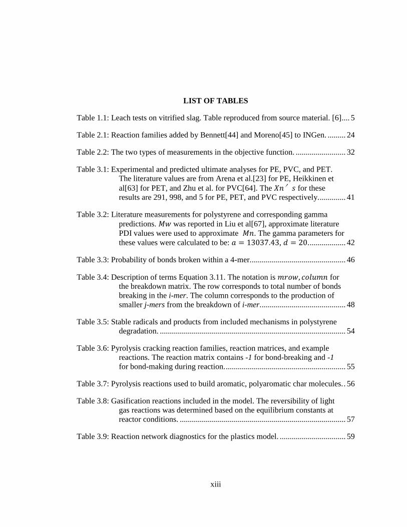
Table 1.1: Leach tests on vitrified slag. Table reproduced from source material. [6] .... 5

Table 2.1: Reaction families added by Bennett[44] and Moreno[45] to INGen. ......... 24

Table 2.2: The two types of measurements in the objective function. ......................... 32

Table 3.1: Experimental and predicted ultimate analyses for PE, PVC, and PET.

The literature values are from Arena et al.[23] for PE, Heikkinen et

al[63] for PET, and Zhu et al. for PVC[64]. The 𝑋𝑛′𝑠 for these

results are 291, 998, and 5 for PE, PET, and PVC respectively. ............. 41

Table 3.2: Literature measurements for polystyrene and corresponding gamma

predictions. 𝑀𝑤 was reported in Liu et al[67], approximate literature

PDI values were used to approximate 𝑀𝑛. The gamma parameters for

these values were calculated to be: 𝑎 = 13037.43, 𝑑 = 20. .................. 42

Table 3.3: Probability of bonds broken within a 4-mer. ............................................... 46

Table 3.4: Description of terms Equation 3.11. The notation is 𝑚𝑟𝑜𝑤, 𝑐𝑜𝑙𝑢𝑚𝑛 for

the breakdown matrix. The row corresponds to total number of bonds

breaking in the i-mer. The column corresponds to the production of

smaller j-mers from the breakdown of i-mer. .......................................... 48

Table 3.5: Stable radicals and products from included mechanisms in polystyrene

degradation. ............................................................................................. 54

Table 3.6: Pyrolysis cracking reaction families, reaction matrices, and example

reactions. The reaction matrix contains -1 for bond-breaking and -1

for bond-making during reaction. ............................................................ 55

Table 3.7: Pyrolysis reactions used to build aromatic, polyaromatic char molecules. . 56

Table 3.8: Gasification reactions included in the model. The reversibility of light

gas reactions was determined based on the equilibrium constants at

reactor conditions. ................................................................................... 57

Table 3.9: Reaction network diagnostics for the plastics model. ................................. 59

LIST OF TABLES

xiv

Table 3.10: Utilized experiments from Arena et al[23]................................................ 62

Table 3.11: HCl and char from all experiments in Slapak et al.[82] Q1 and Q2 are

uncatalyzed (quartz sand bed). A1, A2, and all A3 experiments were

under alumina support. *- data points not used in char analysis due to

catalyst effects on char formation. .......................................................... 68

Table 3.12: Experimental weight percent values for monoaromatics, diaromatics

and triaromatics in pyrolysis output at different temperatures[67]. All

values are in weight percent of initial polystyrene. ................................. 70

Table 3.13: Reaction family rate constants at 1000 K relative to Acylic Thermal

Cracking. log(k)relative,1000=log(k)AcylicThermalCracking,1000-

log(k)ReactionFamily,1000. ............................................................................... 71

Table 4.1: Ultimate analysis of cellulose samples in Chang et al. (2011)[99]. ........... 81

Table 4.2: Comparison between experimental data and predictions from the Linear

Polymer Composition Editor. Experimental data came from Chang et

al.[99] and Couhert et al.[100], [101] for cellulose and hemicellulose,

respectively. The simulated average degree of polymerizations for

cellulose and hemicellulose were 232 and 5. .......................................... 83

Table 4.3: C9 units of Lignin[103]. .............................................................................. 84

Table 4.4: Attribute Identities as parsed by CME from the Freudenberg model for

lignin. ....................................................................................................... 87

Table 4.5: Mole fraction calculation from sampled molecules. ................................... 89

Table 4.6: Experimental Data used in the optimization of the lignin compositional

model. All data are from Hage et al. (2009)[104]. .................................. 90

Table 4.7: Adjustable parameters in optimization. *obtained by difference, not an

adjustable parameter. In simulations 1 and 2, bolded terms were

optimized on. ........................................................................................... 92

Table 4.8: Experimental data currently used in the optimization of the lignin

compositional model. All data are from Hage et al. (2009)[104]. The

data shown here is a subset of data reported; CME adjustments are

required to make use of more data. ......................................................... 93

Table 4.9: Ultimate analysis for each subcomponent of biomass from preceding

sections. ................................................................................................... 94

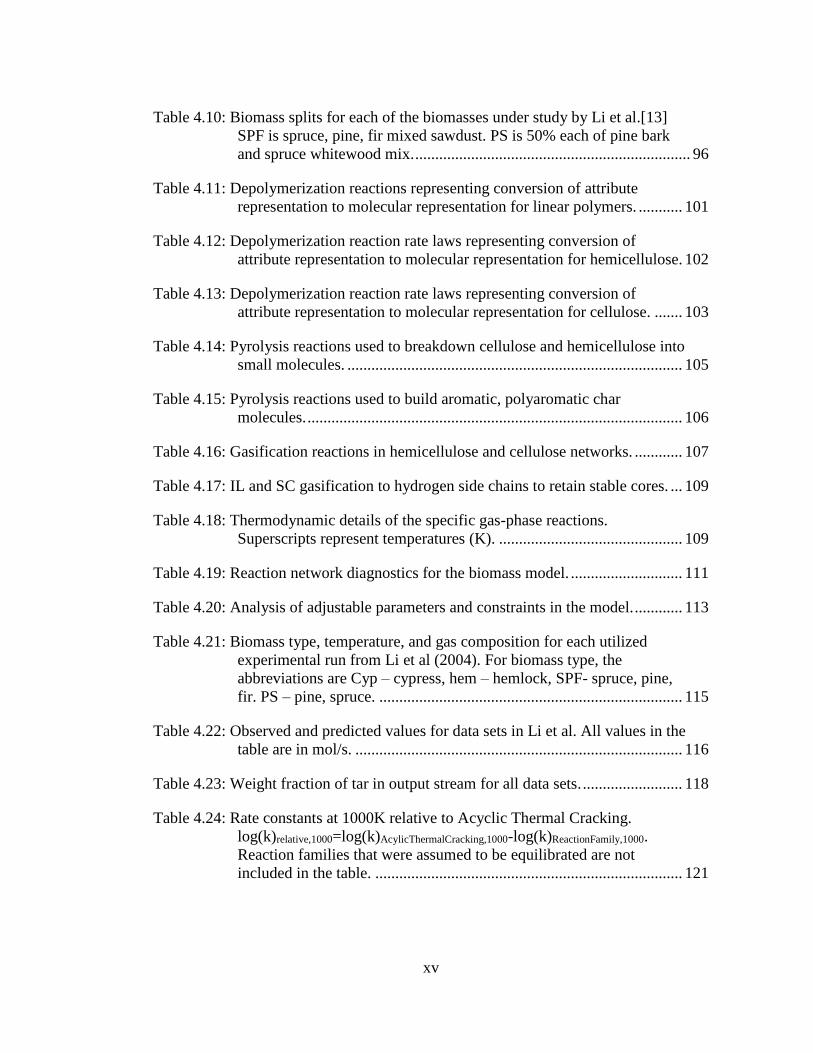
xv

Table 4.10: Biomass splits for each of the biomasses under study by Li et al.[13]

SPF is spruce, pine, fir mixed sawdust. PS is 50% each of pine bark

and spruce whitewood mix. ..................................................................... 96

Table 4.11: Depolymerization reactions representing conversion of attribute

representation to molecular representation for linear polymers. ........... 101

Table 4.12: Depolymerization reaction rate laws representing conversion of

attribute representation to molecular representation for hemicellulose. 102

Table 4.13: Depolymerization reaction rate laws representing conversion of

attribute representation to molecular representation for cellulose. ....... 103

Table 4.14: Pyrolysis reactions used to breakdown cellulose and hemicellulose into

small molecules. .................................................................................... 105

Table 4.15: Pyrolysis reactions used to build aromatic, polyaromatic char

molecules. .............................................................................................. 106

Table 4.16: Gasification reactions in hemicellulose and cellulose networks. ............ 107

Table 4.17: IL and SC gasification to hydrogen side chains to retain stable cores. ... 109

Table 4.18: Thermodynamic details of the specific gas-phase reactions.

Superscripts represent temperatures (K). .............................................. 109

Table 4.19: Reaction network diagnostics for the biomass model. ............................ 111

Table 4.20: Analysis of adjustable parameters and constraints in the model. ............ 113

Table 4.21: Biomass type, temperature, and gas composition for each utilized

experimental run from Li et al (2004). For biomass type, the

abbreviations are Cyp – cypress, hem – hemlock, SPF- spruce, pine,

fir. PS – pine, spruce. ............................................................................ 115

Table 4.22: Observed and predicted values for data sets in Li et al. All values in the

table are in mol/s. .................................................................................. 116

Table 4.23: Weight fraction of tar in output stream for all data sets. ......................... 118

Table 4.24: Rate constants at 1000K relative to Acyclic Thermal Cracking.

log(k)relative,1000=log(k)AcylicThermalCracking,1000-log(k)ReactionFamily,1000.

Reaction families that were assumed to be equilibrated are not

included in the table. ............................................................................. 121

xvi

Table 5.1: Pyrolysis reaction families in MSW gasification. These families include

both categories of pyrolysis chemistry: cracking and tar-formation.

This table was adapted from tables in prior work[54], [83]. ................. 133

Table 5.2: Included gasification reactions. Table is directly from Horton et al[54]. . 134

Table 5.3: Ultimate analysis of coke fed to the gasifier. ............................................ 136

Table 5.4: Reaction network for the coke gasification model. Definitions: 𝑐𝑅 =𝐶𝑂𝐶𝑂2 𝑟𝑎𝑡𝑖𝑜, 𝑟𝑛𝑒𝑡 is the net rate taking into account both intrinsic

kinetics and diffusional limitations. 𝐶0, 𝐻0, 𝑆0, 𝑁0 are the relative

initial amounts of each element in the coke (Units in either Mol/s or

Mol/L). .................................................................................................. 140

Table 5.5: Comparison of MSW compositions. All data points used equivalence

ratio of 0.3. The syngas flow rate was defined as the flow rate sum of

CO, CO2, H2, and CH4. Relative syngas flow rate was the ratio of the

flow rate to minimum flow rate amount the data sets. .......................... 154

Table 6.1: The mole fraction calculation for selected molecules from attributes.

Pcore, PIL, and PSC represent the three attribute PDFs. PBS and PCS

represent the binding site and cluster size distributions. ....................... 164

Table 6.2: Number of molecules for the two common sampling methods for

different cluster sizes using 100 cores, 2 linkages, and 50 side chains. 165

Table 6.3: Cracking reaction families, sites, matrices, and examples. These details

are discussed in the PhD Thesis by Zhang[130]. The reaction matrices

define the bond making (1) and bond breaking (-1) in a reaction type. 172

Table 6.4: Aromatization reaction families, sites, matrices, and examples for

aromatization reactions. These details are discussed in the PhD Thesis

by Zhang[130]. ...................................................................................... 173

Table 6.5: Reaction network diagnostics including total number of reactions,

attributes, and irreducible molecules. These details are discussed in

the PhD Thesis by Zhang[130]. ............................................................. 175

Table 6.6: Experimental data for resid pyrolysis at 500 °C and 0.101 MPa for 40

minutes. All data were collected at the State Key Laboratory of Heavy

Oil Processing, China University of Petroleum. ................................... 180

xvii

Table 6.7: Total error and error associated with experiments and quantitative

structure property correlations for the measurements in the objective

functions. Values for error were estimated based on experience in our

prior work[46] with similar data in the objective function. .................. 182

Table 6.8: Tuned parameters for kinetic model for each reaction family. aj=ln(Aj)-

E0(j)/RT and bj=-αj/RT. For aromatic ring condensation, αj is the

scaling factor, as shown in Equation 6.7. The value for the gas

constant used is R=1.987*10-3 kcal/(mol*K) and T=773 K. ................ 184

Table 7.1: The types and goals of kinetic model users. .............................................. 189

Table 7.2: The categories of apps as organized by objective, corresponding design

method, and a list of apps developed .................................................... 192

Table 7.3: The KMT software supported by each App discussed in this thesis. ........ 193

Table 7.4: Information types, relevant KMT software, how the information is

organized, and how well the user comprehends the information. *the

comprehension of the reaction network depends on the network size. . 198

Table 7.5: Ethane pyrolysis reaction network before and after seeding. .................... 204

Table 7.6: Reaction rate information from KME. ...................................................... 205

Table 7.7: Apps excluded from the current chapter. .................................................. 213

Table 7.8: Block Types and Descriptions included in KME Flowsheet Application. 216

Table 7.9: Some common molecules divided into Benson Groups and predicted

heats of formation versus the values found in the NIST database. ....... 222

Table 7.10: Order of preference for sources of molecular properties. ....................... 223

Table 7.11: Inputs, observed quantities, minimum and possible values at reactor

outlet, and whether a heuristic returns a red flag. ................................. 227

Table 8.1: Experimental[64] and predicted ultimate analyses for PVC. Also given

are the ultimate analyses if the for a monomer and infinite polymer,

and pure polyene structure. The partially depolymerized polymer was

93.6% PVC repeat units with 6.4% polyene repeat units. ..................... 233

xviii

Figure 1.1: MSW management technologies from 1960-2013. Figure from source

material[1]. ................................................................................................ 2

Figure 1.2: Net energy to grid per ton of MSW. Figure reproduced from source

material[6]. ................................................................................................ 4

Figure 1.3: Alter NRG Plasma Gasifier. Image from source[6]. .................................... 7

Figure 1.4: MSW breakdown in 2013 for the United States[1]. This composition

represents the discarded (i.e., post-recycling) MSW. ................................ 8

Figure 1.5: Urban and rural MSW waste descriptions in the United Kingdom[25]. ...... 8

Figure 1.6: Artificial Neural Net from Xiao and coworkers. Image directly from

source material[37]. ................................................................................. 11

Figure 2.1: CME Optimization loop which converts available experimental

measurements to a molecular composition. ............................................ 18

Figure 2.2 Bond electron matrix representation of propan-1-ol from Moreno[45].

Figure from source material. ................................................................... 19

Figure 2.3: Generalized Alcohol Dehydration Reaction. ............................................. 21

Figure 2.4: Cellulose monomer, glucose. ..................................................................... 21

Figure 2.5: alcohol dehydration of propan-1-ol to propene and water. ........................ 25

Figure 2.6: Chemical reaction as a matrix operation for propan-1-ol dehydration.

Figure from source material[45]. ............................................................. 26

Figure 2.7: Separation of the full bond electron matrix post-reaction into product

molecules. ................................................................................................ 26

Figure 2.8: Figure from Horton and Klein[47]. (a) Figure reproduced Mochida and

Yoneda[49] showing the dealyklation of alkylaromatics reaction

family on a SA-1-Na-3 catalyst. The numbers represent experimental

rates of dealkylation on different alkyl aromatics. .................................. 30

LIST OF FIGURES

xix

Figure 2.9: Example parity plot for the pyrolysis of naphtha for an experimental

carbon number distribution. Figure from source material[42]. ............... 33

Figure 3.1: Plastics generation and recovery from the EPA report on Municipal

Solid Waste (MSW)[1]. ........................................................................... 37

Figure 3.2: Repeat Unit Structures for PE, PVC, PET, and PS (Left to Right). .......... 39

Figure 3.3: Conceptual goal of random scission for a generalized polymer size

distribution. Top and bottom figures are representative n-mer

distributions. ............................................................................................ 45

Figure 3.4: Illustration (top) and breakdown matrix representation (bottom) of

possible bond breaking events in a 4-mer. Values in the matrix are

relative initial amount of 4-mer. .............................................................. 47

Figure 3.5: Radical propagation steps for polyethylene depolymerization. The H-

abstraction step shown here is inter-molecular and can occur with any

radical in the system. ............................................................................... 49

Figure 3.6: Oligomers with 6-carbons produced during polyethylene

depolymerization. These are the starting molecules from polyethylene

for the full pyrolysis and gasification network. ....................................... 50

Figure 3.7: Link cleavage in polyethylene terephthalate (concerted mechanism). ...... 51

Figure 3.8: Two-step depolymerization of polyvinyl chloride. .................................... 52

Figure 3.9: Tuning results for all data sets. The linear fit has the equation

ypredicted=0.952*yexperimental+0.0036. Tar yield is in units of (g/s/25); it

was rescaled to have a similar value as the light gas flow rates (mol/s). 63

Figure 3.10: Comparison of experimental and model predicted results for liquid/gas

ratio (mass basis) for all data sets. ........................................................... 63

Figure 3.11: Experimental error and the effects of temperature deviation in model

predictions for Run 6. Effects of a 10 degree temperature variation are

shown using error bars. ........................................................................... 64

Figure 3.12: Logic for the TGA Simulator C# application .......................................... 65

xx

Figure 3.13: TGA model results (lines) compared with experiment (points). Colors

correspond to different heating rates: red, 5 °C/min; green, 10 °C/min;

blue, 20 °C/min; orange, 40 °C/min. The left plot gives the TGA

curves, the right plot is a parity plot of the results. The maximum

decomposition rates in units of wt%/°C are 0.018, 0.17, 0.015, and

0.041 in order of increasing heating rate. ................................................ 66

Figure 3.14: TGA Simulator results showing persistence of char in the absence of

oxygen for PET depolymerization at a heating rate of 40 °C/min. ......... 67

Figure 3.15: Results for HCl (all runs) and Char (only Q1 and Q2). The outlet flow

rate units for HCl and char are in mol/s and g/s/50 respectively. ........... 69

Figure 3.16: Parity plot for monomer-trimer predictions for polystyrene pyrolysis.

A least-squares linear fit of the data gives ypredicted = 0.9595yexperimental

+ 0.0217 ................................................................................................... 70

Figure 4.1: Literature lumped kinetic models. (Left) Sequential lumped model[86]

of biomass gasification. (Right) parallel lumped model of biomass

gasification where V1-V5 are lumped volatile products.[87] .................. 76

Figure 4.2: Cellulose polymeric n-mer of 𝛽1 → 4 linked D-glucose units (Left).

Hemicellulose representation as an n-mer of poly-xylan (Right). .......... 79

Figure 4.3: Linear Polymer Composition Editor optimization loop. ............................ 82

Figure 4.4: Adapted Freudenberg Structure[102]. This structure was parsed to yield

the attribute identities. ............................................................................. 85

Figure 4.5: Binding site types on the phenol core. ....................................................... 88

Figure 4.6: Logic of MSW Bulk Composition solver applied for biomass. All

numbers in this figure are in wt%. The plastics and carbon support

segments of the figure are truncated as the weight fraction within

biomass is 0 for each. *-Lignin fraction is dependent on cellulose and

hemicellulose. .......................................................................................... 95

Figure 4.7: Cellulose Depolymerization Pathways. ..................................................... 98

Figure 4.8: Complete cracking of a cellulose 4-mer showing final monomeric

products. .................................................................................................. 98

Figure 4.9: Starting molecules of full cellulose pyrolysis network: linear

levoglucosan (left) and linear glucose (right). ......................................... 99

xxi

Figure 4.10: Depolymerization pathways for hemicellulose. ..................................... 100

Figure 4.11: Linear forms of anhydro-xylopyranose (left) and xylose (right). These

are the starting point of the full pyrolysis network. .............................. 100

Figure 4.12: Example of stepwise gasification reactions of cores. Each reaction is

written for both incomplete combustion and steam reforming. The

alternate reactions where the phenol ring is gasified first were also

written. ................................................................................................... 108

Figure 4.13: Parity plot of tuned data sets for Li et al data. After a linear fit, the

formula comparing experiment to model results is

ypredicted=yobs*0.928+0.0003. The R2 relative to y=x is 0.918 for the

tuned data sets. ...................................................................................... 116

Figure 4.14: All viable datasets from Li et al (2004) using tuned parameters from

data sets 3, 4, and 11. Squares represent tuned results, circles are

predicted results. After a linear fit, the formula comparing experiment

to model results is ypredicted=yobs*0.989-0.007. The R2 relative to y=x is

0.861 for all data sets. ............................................................................ 117

Figure 4.15: Tar weight fraction as a function of the ratio of dry biomass to

supplied oxygen (blue, left axis). The fraction of CO and H2 in overall

dry syngas (nitrogen excluded) is also shown (orange, right axis). ...... 119

Figure 4.16: Relative importance of reaction families in the reactor model

integration for Data Set 11. All analysis was done using an in-house

C# application, KME Results Analyzer. ................................................ 120


material[1]. ............................................................................................ 125

Figure 5.2: Average landfill tipping fees in the US 1982-2013. Prices are in

USD.[1] ................................................................................................. 126

Figure 5.3: MSW Fractions in the United States in 2013. A. Overall fractions as

reported by the EPA. B. MSW divided into four categories. The

biomass-derived category includes food, wood, yard trimmings,

textiles, and paper. The ‘not modeled’ category includes metals, glass,

other, and rubber and leather. C. the cellulose hemicellulose and lignin

splits predicted in prior work[83] using data from Li and

coworkers[13]. D. The relative amounts of included plastics,

renormalized from EPA data[1]. ........................................................... 130

xxii

Figure 5.4: Screenshot from the MSW Bulk Composition Solver. In this screen, the

checkboxes on the left allow the user to select which fractions are

adjusted during the optimization procedure. ......................................... 131

Figure 5.5: Comparison of initial reaction rates for 4” (top) and 6” (bottom)

particles for gasification with oxygen. Data labels give values for

diffusion limitations at 1200K to show comparison in particle sizes. ... 143

Figure 5.6: Damköhler number as a function of temperature for 4” and 6” particles.144

Figure 5.7: Reaction rate contributions as a function of temperature for CO2

gasification from the Cupula Handbook[121]. In the low temperature

region (w1), kinetic limitations dominate. The middle range

temperatures, w2, both kinetics and diffusion contribute to the overall

rate. At high temperatures (w3), diffusional limitations dominate. ....... 145

Figure 5.8: Gasification unit depiction from Young[6] (left) and conceptual

organization of idealized reactors for each reaction zone(right). .......... 145

Figure 5.9: Screenshot of the main screen from the MSW Gasification I/O

Converter. Measurable process inputs are on the left, the reactor

layout is given in the diagram, and measurable process outputs are on

the right. ................................................................................................. 147

Figure 5.10: Edit MSW Composition window within the MSW User Friendly

Gasification Model. ............................................................................... 149

Figure 5.11: Tar composition analysis screen in the MSW Gasification I/O

Converter. .............................................................................................. 149

Figure 5.12: Relative tar fraction and relative syngas quality as a function of

equivalence ratio. The tar fraction is defined as the weight fraction of

species with boiling point greater than or equal to benzene. Syngas

quality here is the mass ratio of CO+H2 to CO+H2+CH4+CO2. ........... 151

Figure 5.13: Tar composition leaving the freeboard zone. Left: overall tar molecule

mass fractions. Right: composition of lignin tar molecules. ................. 152

Figure 5.14: Seasonal Dependence of UK MSW, winter and summer[25]. .............. 153

Figure 5.15: Comparison of Tar Compositions for different MSW compositions:

Left(UK-Summer), Right(Synthesized 2). ............................................ 154

xxiii

Figure 5.16: Effect of 𝛼 on relative syngas quality (orange) and tar flow rate (blue)

at equivalence ratios of 0.4 (top) and 0.3 (bottom). .............................. 155

Figure 6.1: Comparison of Attribute Reaction Modeling and Conventional

Modeling methods. ................................................................................ 162

Figure 6.2: Example resid molecule and attribute groups: cores (blue), inter-core

linkages (red), and side chains (green). ................................................. 163

Figure 6.3: Differences in binding sites for complete sampling and main methyl

method. .................................................................................................. 166

Figure 6.4: Examples of both hydrocarbon and heteroatom-containing core

attributes. ............................................................................................... 167

Figure 6.5: The four side chain types and two inter-core linkages. The side chain

types are, top-to-bottom, n-alkyl, iso-alkyl, carboxylic acid, and

sulfide. ................................................................................................... 167

Figure 6.6: Side chain (left) and Inter-core linkage (right) PDFs. The side chain

PDF is only shown for n-alkyl side chains (normalized to 1). Similar

PDFs can be created for the other side chain types. .............................. 168

Figure 6.7: Selected cores from the core PDF, mole fractions normalized for the

selected cores. ........................................................................................ 169

Figure 6.8: Binding site (left) and cluster size (right) PDFs for feedstock

composition. Results are from model presented by Zhang et al.[46] .... 169

Figure 6.9: Molecular weight distribution of the sampled molecules. Figure

reproduced from attribute distributions in Zhang et al[46]. .................. 170

Figure 6.10: Most stable cracking pathways for an alkyl aromatic. ........................... 171

Figure 6.11: Aromatic ring condensation example reaction. ..................................... 174

Figure 6.12: Conversion of continuous attribute pdfs to discrete PDFs during the

generation of initial conditions for the reactor kinetic model. .............. 177

Figure 6.13: The alteration of attribute PDFs through model solution. ..................... 178

xxiv

Figure 6.14: Parity plot comparing experimental and predicted results. The y=x line

corresponds to exact prediction. All weight percent values were

converted to weight fractions, the average molecular weight for gas-

oil was normalized to be on the same scale as other data. The R2 value

relative to y=x is 0.944. ......................................................................... 183

Figure 6.15: Observed versus experimental including error bars for σtotal; the error

bars were chosen to be drawn on the experimental values. The average

molecular weight for gas-oil was normalized to be on the same scale

as other data. .......................................................................................... 184

Figure 6.16: Before (left) and After(right) distributions for MW, aromatic ring

number, and naphthenic ring numbers. ................................................. 186

Figure 7.1: Main software packages that make up the Kinetic Modeler’s Toolkit .... 190

Figure 7.2: (Left) Typical lumped model of coal pyrolysis. (Right) Conceptual

representation of the information complexity in coal pyrolysis versus

simple lumped models. .......................................................................... 194

Figure 7.3: Trade-offs of the comprehension and scientific rigor of models as a

function of the number of equations. ..................................................... 195

Figure 7.4: Information sources and amounts within a molecular-level kinetic

model. Values are relative and qualitative. The relatively low value

for rate parameters is due to a linear free energy relationship (LFER)

basis. ...................................................................................................... 196

Figure 7.5: Sample screenshot from the Reaction Network Visualizer. Graph image

rendered using GraphViz[132]. ............................................................. 199

Figure 7.6: Reaction families and some example reactions from ethane pyrolysis.

The primary form of mass increase from ethane is first via olefin

addition reactions. Once large olefins form, Diels-alder additions

allow for the formation of cyclic structures. Beta-scission can then

lead to aromaticity and the product of interest, xylene. ........................ 201

Figure 7.7: Number of equations by rank in an ethane pyrolysis model with ethane

as the only seed. The black dots represent the location of xylenes

before and after seeding. ....................................................................... 202

Figure 7.8: Some major reaction paths visualized using the Reaction Network

Visualizer. Images rendered using GraphViz. ....................................... 203

xxv

Figure 7.9: Full reaction network generation in a Naphtha Reforming model. ......... 206

Figure 7.10: Reaction families responsible for the production of 3-methyldecane. .. 207

Figure 7.11: Visualization of Bulk Properties in the KME Results Analyzer ............ 208

Figure 7.12: Window allowing the addition of bulk properties to the KME Results

Analyzer. The bulk property added here is 1-3 ring aromatics. ............ 209

Figure 7.13: Sample Screenshot from the MSW Gasification I/O Converter. ........... 210

Figure 7.14: Sample Screenshot from Naphtha Reforming I/O Converter ................ 212

Figure 7.15: Sample screenshot from the KME Flowsheet Application. The

flowsheet layout images in the KME Flowsheet Application are

rendered using the open-source GraphViz software[132]. .................... 214

Figure 7.16: Solution order of blocks in the example flowsheet. ............................... 217

Figure 7.17: Conceptual Diagram of a Thermogravimetric Analysis experiment. .... 218

Figure 7.18: Selected screenshots from TGA Simulator. Upper Left: opening screen

where user can select the KME model. Upper right: Experimental data

Input. Lower Left: simulation settings. Lower right: results and

comparison with experiments. ............................................................... 219

Figure 7.19: TGA Simulator Logic. Image from source [54]. ................................... 220

Figure 7.20: Boiling point options in TGA Simulator ............................................... 220

Figure 7.21: Screenshot of Physical Property Database Interface. ............................ 224

Figure 7.22: Export molecule list window in the Physical Property Database

Interface. The left side shows a search of the database for all species

with 1 or more aromatic ring. The right side gives the current list of

selected molecules and details on which properties are being exported.225

Figure 7.23: Basic reaction network layout for heuristic example. ............................ 227

Figure 7.24: Comparison of user interfaces in Windows Forms Applications (Left,

App: INGen Network Merge) and Windows Presentation Foundation

(WPF, Physical Properties Database Interface). ................................... 229

xxvi

Figure 8.1: 95% confidence intervals on A-factors relative to the value of the A-

factor. For instance, the confidence interval is ±0.169 ∗ 𝑙𝑜𝑔𝐴 for

dehydrogenation. ................................................................................... 236

Figure 8.2: Comparison of DBE versus Carbon Number for single pyrollic ring

structures for experimental(right) and predicted (left) results. Figure

taken directly from source and was Figure 15 in the source

material.[46] .......................................................................................... 238

Figure A.1: RightsLink permission obtained from ACS for reproduced work

published by author[47]. ........................................................................ 252






published by author[109]. ...................................................................... 254

xxvii

Municipal Solid Waste (MSW) is a valuable energy resource that is

underutilized by today’s society. Waste-to-Energy (WTE) is a low-hanging fruit in a

multifaceted energy landscape that incorporates conventional fuels and a plethora of

renewable alternatives. From an environmental standpoint, WTE reduces the storage

of MSW in landfills which can contaminate groundwater and release methane, a

potent greenhouse gas. The most attractive WTE technology is gasification, a process

where nonstoichiometric amounts of oxygen or air are fed to a high temperature

reactor. The output from gasification is syngas, a ubiquitous product that can be used

for a range of purposes, including liquid fuel synthesis and conversion to electricity

via combustion. Plasma-arc gasification is an extension of conventional gasification

that utilizes a plasma torch to obtain extreme reactor temperatures. The solid by-

product from plasma gasification is an inert vitrified slag, which is usable as a

construction material. Plasma-arc gasification successfully utilizes the entire MSW

feedstock, thereby removing the need for landfills. However plasma-arc gasification is

a relatively new WTE technology, and there is a need to better understand the

underlying chemistry in order to optimize process parameters.

Molecular-level kinetic modeling has proven valuable in gaining insight on

process chemistries ranging from naphtha reforming to biomass pyrolysis. To this end,

this dissertation focuses on the development and application of a molecular-level

kinetic model for MSW gasification. For model development, the MSW stream was

divided into plastics and biomass. Kinetic models were constructed separately for the

ABSTRACT

xxviii

gasification of each of these streams, using literature data. These models were then

combined to construct the MSW gasification model. This model was used to simulate

a 1000 metric ton per day plasma-arc gasifier that was divided into three zones for

MSW: combustion, gasification, and freeboard. The reactor model was utilized to

study the effects of process parameters on syngas quality and tar formation. Increasing

the relative oxygen flow to the bed was found to reduce tar formation at the cost of

syngas quality. Variations in MSW composition affected the oxygen content in tar

molecules but had little impact on syngas quality. Lastly, the localized extreme

temperatures in the combustion zone had a potentially negative impact on both syngas

quality and tar production due to the oxidation of CO.

While studying MSW gasification, modeling approaches were developed for

the depolymerization of both linear and cross-linked polymers that could be applied to

other complex feedstocks and processes. In particular, this dissertation focuses on

heavy oil resid pyrolysis. Resid pyrolysis is an attractive field for modeling due to

recent advances in experimental techniques. This study highlighted the ability of

molecular-level kinetic models to predict >50,000 molecules from detailed mass

spectrometry measurements.

Orthogonal to kinetic model development, this thesis focused on the

construction of software tools. Software tool development highlighted the interface

between molecular-level kinetic models and users. There are three types of users of

kinetic models: model developers, research collaborators, and process engineers. Each

user has their own goals while using the model. For instance, software tools for model

developers or research collaborators might focus on organizing the incredible amount

of information contained in a molecular-level kinetic model. To address this aim, one

xxix

tool focused on the visualization of the reaction network to understand the network

structure. In contrast, software tools designed for process engineers target measured

inputs and outputs while abstracting the underlying molecular detail. This allows a

process engineer, regardless of training in detailed kinetics, to reap the benefits of a

molecular model and study the effects of operation parameters such as temperature or

feed variation. These examples showcase the ability of software tools to increase the

accessibility of detailed kinetics by molding the user-model interface to correspond to

the user’s needs.

This dissertation focused on gasification of waste, and culminated in a reactor

model for the most environmentally friendly of WTE option: plasma-arc gasification.

This work was then taken one step further by developing the software necessary to

increase the accessibility of the model to a wider audience, ranging from process

engineers to model developers. This accessibility makes the model not only

fundamental, but also practical for industrial partners. Gasification and other WTE

technologies have been, and will continue to be, a future topic of research.

Undoubtedly, detailed kinetic models will play a central role in the future conversion

of waste to energy

1

INTRODUCTION

1.1 Municipal Solid Waste: Burden or Resource?

By its very designation, municipal solid waste (MSW) is viewed as a problem

in today’s society. The term waste, as defined by the Oxford dictionary, is a “material

that is not wanted; the unusable remains or byproducts of something.” Historically,

this term was valid; according to the Environmental Protection Agency (EPA),

essentially all MSW in the United States was placed in landfills before 1960, as shown

in Figure 1.1[1]. Landfills can have issues in terms of the environment and public

perception. First, waste stored in landfills can contaminate groundwater. Second,

waste degradation by microbes in landfills produces methane[2], a greenhouse gas

with a global warming potential roughly 25 times higher than carbon dioxide[3].

Additionally, in terms of public perception, landfills are an eyesore. They are one of

the most common examples of the NIMBY, or “not in my backyard”, effect. MSW

that is discarded in landfills truly merits being called waste.

Chapter 1

2


material[1].

Beginning around 1970, society began ways to utilize MSW. Between 1970

and 2000, there was a gradual increase in the fraction of waste recovered for recycling.

Furthermore, in this time period, industry began to realize that MSW contains

considerable energy, giving rise to combustion as the first waste-to-energy technology

to be used at the industrial scale. Today, around half of MSW still goes to landfills,

where this energy source is left untapped. The energy landscape in a modern society is

quickly becoming multi-faceted, involving renewables, traditional fuels, and nuclear

power. In this landscape, waste-to-energy is a low-hanging fruit requiring little

research to obtain significant results. Other countries have utilized this resource; for

example, Sweden made news in 2015 because they transport trash to fuel waste-to-

energy facilities from surrounding countries[4]. If this is any indication of the future

of MSW in the United States, it will be considered a resource, rather than waste.

3

1.2 Waste-to-Energy Technologies

There are numerous waste-to-energy (WTE) technologies that are currently

feasible. These technologies include methane recovery from landfills, incineration,

gasification, and plasma-arc gasification. Each of these technologies has advantages

and disadvantages in terms of environmental concerns, energy obtained, and ease of

implementation.

Methane recovery from landfills, also called landfill gas, is a WTE technology

that focuses on waste after it has been deposited in landfills. There are two benefits.

First, the methane can be burned to generate energy. Second, capturing and burning

methane produces CO2, a much less potent greenhouse gas. This technology is being

actively pursued in the United States. According to the EPA, 645 landfills have been

retrofitted to recover methane for energy production (as of March 2015), generating

power for 1.2 million homes with 440 candidate landfills for future development[3].

Landfill gas recovery is a good short-term technology for obtaining energy

from landfilled MSW; however, there are many drawbacks. First, all other

disadvantages of landfills (e.g., potential groundwater contamination) still exist. It is

difficult to compare the energy obtained from landfill gas to other WTE technologies

due to differences in timescales. Methane recovery is dependent on the rate at which

microbes break down the material, which is significantly longer than the other

techniques. Intuitively, the total energy recovered from a slow, partial breakdown via

microbes is lower than a fast, near-complete breakdown by any other WTE

technology. For these reasons, WTE technologies that minimize, or even exclude, the

use of landfills are better long-term solutions.

The oldest, and currently most popular, WTE technology is incineration. This

process entails the complete combustion of waste: excess oxygen is fed to the process,

4

which converts the waste entirely to CO2. The heat from this process is utilized to

generate electricity. The inherent simplicity of this process is compromised by the

production of ash and pollutants. Of the original waste, 20-30% is categorized as non-

hazardous ash and 2-6% as hazardous ash[5]. Incinerator ash is typically deposited in

landfills[6]. The excess oxygen also promotes the formation of SOx, NOx, dioxins, and

furans[7]. Laws such as the Clean Air Act[8] regulate the release of pollutants into the

atmosphere, and incineration facilities must be designed to meet these standards.

Figure 1.2: Net energy to grid per ton of MSW. Figure reproduced from source

material[6].

Gasification addresses many of the issues with incineration by reducing the

oxygen flow to the bed. The final product is a syngas—or synthesis gas—stream

predominantly composed of CO and H2. This ubiquitous outlet can be used to create

chemicals or liquid fuel. Most often, however, the syngas stream is burned to generate

electricity. Gasification has been applied extensively to more conventional feedstocks,

e.g., coal[9]–[12] or biomass[13]–[20]. This process is more efficient than

0

100

200

300

400

500

600

700

800

900

Incineration Gasification Plasma-arcGasification

kWh

r/to

n M

SW

5

incineration, which is reflected in the larger net energy to grid per ton of MSW, as

shown in Figure 1.2[6]. In conventional gasification, the final solid by-product of

gasification is an ash material that ends up in landfills.

The ash byproduct from gasification has been addressed in a more recent type

of gasifier that utilizes a plasma torch. This technique, termed “plasma-arc

gasification”, melts the ash at extreme temperatures in the gasification bed, that can

exceed 7000 °F[6]. The final solid byproduct is a vitrified slag which passes

groundwater leach tests (shown in Table 1.1) and can be utilized as a construction

material. The major disadvantages of plasma-arc gasification are capital costs for a

new facility and the risks associated with new technologies. Plasma-arc gasification is

the only technology currently in use that completely removes the need for landfills.

Table 1.1: Leach tests on vitrified slag. Table reproduced from source material. [6]

EPA Permissible

Conc. (mg/L)

Vitrified Slag Conc.

(mg/L)

Arsenic 5 <0.1

Barium 100 0.47

Cadmium 1 <0.1

Chromium 5 <0.1

Lead 5 <0.1

Mercury 0.2 <0.1

Selenium 1 <0.1

Silver 5 <0.1

1.3 Plasma-Arc Gasification

A general plasma-arc gasification reactor is depicted in Figure 1.3. MSW is fed

near the middle of the gasifier. The waste falls and forms a bed in the gasification

zone. Along the height and circumference of this bed are inlets for the gasification

6

agent: typically air, oxygen-enriched air, or pure O2[21]. The zone of open space

above the MSW bed is called the freeboard zone, where primarily equilibrium

reactions, such as water-gas shift, occur. After the freeboard zone, syngas leaves the

top of the reactor. The other output is the vitrified slag, which exits the bottom of the

gasifier and is molten at reactor conditions. In the diagram, the plasma torch is shown

inside the gasifier; however, it can also be separate. In this scenario, a vapor stream

carries the heat from the torch to the gasifier bed[22].

There are multiple categories of plasma-arc gasification units, but they

generally fall into two categories: one-stage and two-stage. The category described

here, and studied in this thesis, is an example of a one-stage gasifier. Two-stage

examples include multi-reactor designs where the initial waste is fed to a conventional

gasification unit. The plasma gasifier can then be used to convert the tar molecules in

syngas or vitrify the ash into slag.

The primary product from the process is syngas. Depending on reactor

conditions, this syngas can contain measurable amounts of tar molecules, defined here

as molecules with higher boiling points than benzene. These tar molecules must be

processed in downstream units[23]. The quality of the syngas is dependent on the

gasification medium. The energy content, on a per volume basis, can be doubled with

oxygen-enriched air or pure oxygen instead of natural air. This increased energy

density allows for the use of a wider range of gas turbines to make electricity[21].

Syngas composition is dependent on the original feedstock[24], MSW. Most of the

complexity and variability of the process is in the MSW inlet stream.

7

Figure 1.3: Alter NRG Plasma Gasifier. Image from source[6].

The main inlet to the plasma-arc gasifier is MSW, a mixed feedstock that can

be broken down into a number of categories as shown in Figure 1.4. The most

interesting thing about this composition is that it is inherently variable. This is

demonstrated using the breakdown of United Kingdom (UK) waste in Figure 1.5[25].

The composition of UK waste is different than the US. Specifically, plastics are a

much higher fraction of waste in the US. This is important as plastics, which are

derived from oil, have lower oxygen content than biomass and therefore have a higher

energy content. Also, even within the UK, the waste composition changes in urban

and rural settings. The complexity and variability of MSW as a feedstock is a major

motivator for process modeling of MSW gasification.

8

Figure 1.4: MSW breakdown in 2013 for the United States[1]. This composition

represents the discarded (i.e., post-recycling) MSW.

Figure 1.5: Urban and rural MSW waste descriptions in the United Kingdom[25].

1.4 MSW Gasification Modeling

The aim of mathematically modeling of a chemical process is twofold:

practical and scientific. The practical application of modeling is in the design and

0

5

10

15

20

25

30

35

Pe

rce

nta

ge (

by

mas

s)

Urban A Urban B Rural

9

control of the commercial reactor. For MSW gasification, the goal of process

engineers is to control syngas production and composition. Modeling can help guide

the choice of process parameters such that the energy content is maximized while high

molecular weight tar molecules are minimized. The scientific application of modeling

is in the understanding of the physics and chemistry of the process. This is more

important to researchers and future projects as it can answer bigger questions about the

process. For example, scientific understanding can be used to design a MSW stream to

increase syngas energy content or control the composition of tar molecules.

The simplest model for gasification is a model based on the assumption of

thermodynamic equilibrium [13], [16], [25]–[32]. By assuming the system reaches

equilibrium, these models assume a reactor outlet composition based on the

temperature of the system. Equilibrium models can handle changes in MSW feedstock

through ultimate analyses. Returning to the aims of modeling gasification, there are a

number of issues with equilibrium models. Equilibrium models do not contain detailed

reactions and cannot help with understanding the underlying chemistry of the

gasification process. Also, at the temperatures in a plasma-arc gasifier, tar molecules

are not predicted at equilibrium. If tar molecules are observed, then the system is not

at thermodynamic equilibrium and reaction kinetics must be taken into account.

The most basic type of kinetic models are lumped models[34], [35]. An

example of a lumped model is given below in Equation 1.1[34], where chemical

reactions are represented simply between lumped categories. A major advantage of

lumped models is the model simplicity; these models are easy to build and understand.

The mathematical solution is also fast, thereby allowing the kinetics to be easily paired

with more complex descriptions of heat and mass transfer. The limitation of lumped

10

models is that they lack detail beyond the definition of the lumps. Each lump in the

model might represent hundreds or thousands of chemical species. For instance, the

model in Equation 1.1 would have trouble answering questions about the effects of

MSW composition on predicted tar composition. In terms of scientific understanding,

lumped models are based on experimental observations; however, they are ill-

equipped to answer molecular-level questions about the formation of particular

product molecules.

𝑓𝑒𝑒𝑑𝑠𝑡𝑜𝑐𝑘 → 𝑔𝑎𝑠 + 𝑝𝑟𝑖𝑚𝑎𝑟𝑦 𝑡𝑎𝑟 + 𝑐ℎ𝑎𝑟 𝑝𝑟𝑖𝑚𝑎𝑟𝑦 𝑡𝑎𝑟 → 𝑔𝑎𝑠 + 𝑠𝑒𝑐𝑜𝑛𝑑𝑎𝑟𝑦 𝑡𝑎𝑟

(1.1)

Artificial neural nets (ANNs) are kinetic models that are based on how neurons

form connections in the brain[36]. Applied to a chemical process, ANN models have

connections from measured inputs to measured outputs as shown in Figure 1.6[37].

The connections formed are based entirely on the data, and ANNs are ideal in the

scenario where there is no knowledge in how inputs become outputs. This

characteristic is also the key weakness of ANN models. Because there is no chemistry

in the model, the model cannot help explain the underlying science of the physical

process.

11

Figure 1.6: Artificial Neural Net from Xiao and coworkers. Image directly from

source material[37].

Molecular models address the weaknesses of lumped and ANN models by

tracking observable molecules in the reactor. The feed is represented as a set of

molecules and mole fractions. These molecules undergo chemical reactions based on

mechanistic and pathways levels of process chemistry. The reaction integration

utilizes the reaction network to obtain the molecular outputs. This type of modeling

inherently addresses the aims of modeling MSW gasification. First, the model can

inform a process engineer of how process conditions impact measured quantities such

as syngas and tar compositions. Second, because the input is molecular, it can account

for the variable nature of MSW. Third, because the reaction network is based on

reaction chemistry, the model conveys an understanding of the underlying science of

gasification.

12

1.5 Research Objectives

There are two orthogonal sets of objectives in this dissertation: developing

models and model-building tools. Due to the relative scarcity of data on plasma-arc

gasification, model development focused primarily on a general reaction model for the

gasification of MSW. This model was later applied to a specific reactor configuration

of a plasma-arc gasification unit. Similar modeling methods were also utilized for the

development of a kinetic model for the pyrolysis of heavy oil. In terms of model-

building tools, this dissertation work has exposed the importance of the user-model

interface for detailed kinetic models.

The primary objective of this research was the development of a molecular-

level kinetic model for MSW gasification. Due to the complexity of MSW as a

feedstock, a three-stage approach was adopted. In the first stage, a kinetic model was

constructed for common mixed plastics; this model was optimized and validated using

literature gasification data on each of the polymers. The second stage of MSW model

development was the construction of a model for biomass gasification. This model

utilized literature data to optimize and probe the predictive ability of the model. The

final stage of MSW gasification model development focused on merging together the

plastics and biomass models. At this stage, the merged model was a general

gasification reaction model and contained the major components of MSW. This

general model was then applied to a specific MSW plasma-arc gasification process.

The resulting reactor model was utilized to perform trending studies on important

process parameters.

The development of the MSW gasification model led to advances in the

modeling framework for linear and cross-linked polymers. These advances are

applicable to other high molecular weight feedstocks such as coal or heavy oil.

13

Although the chemical makeup and physical properties for these feedstocks are

different from MSW, the polymeric complexity can be approached using the same

mathematical tools. Specifically, this dissertation also focuses on the development of a

model for the pyrolysis of a vacuum residue.

The second set of objectives for this dissertation pertained to software tool

development. There are three users of kinetic models: model developers, research

collaborators, and process engineers. Each type of these users has a different aim, and

effective software tools must address these needs. For example, a tool for a process

engineer focuses on measured inputs and outputs to a process. In contrast, tools for

model developers might focus on enhancing the scientific and mathematical

understanding of the model. An example of this is the visualization of a reaction

network to gain in-depth understanding of the network structure. Through this logic, a

completely different style of tool development has arisen. Rather than focusing on

major software packages with many features, this dissertation focuses on single-

purpose ‘apps.’ This style minimizes the learning curve for a given tool and allows for

more fluid and personalized development for users.

1.6 Dissertation Scope

Chapter 2 provides a background on the Kinetic Modeler’s Toolkit (KMT) and

how it is utilized for building kinetic models. The focus of the chapter is on the system

of material balance differential equations that represent the kinetic model. The chapter

discusses the three main steps of molecular modeling: feedstock composition, reaction

network generation, and kinetic model solution.

Chapter 3 develops a kinetic model for the gasification of mixed plastics,

including polyethylene, polyvinyl chloride, polyethylene terephthalate, and

14

polystyrene. Each polymer was simulated as linear with a constant repeat unit

structure. Statistical methods are utilized for the initial breakdown of the polymeric

macromolecules. A pyrolysis and gasification network is developed for the reaction of

small oligomers. The model parameters are optimized for literature data, and

comparisons are made.

Chapter 4 discusses the construction of a kinetic model for the gasification of

biomass. The focus of the work is on three biopolymers: cellulose, hemicellulose, and

lignin. Cellulose and hemicellulose are approximated as linear polymers, and similar

methods are utilized as in the plastics model. Lignin is modeled as a cross-linked

polymer and the structure is modeled using structural attributes. The model is tuned to

literature data across different biomass types. The predictive ability of the model was

probed using additional data.

Chapter 5 combines the kinetic models of plastics and biomass gasification to

develop a model for MSW gasification. A model for coke gasification is also

developed. The MSW and coke reaction models are applied to a plasma-arc gasifier.

The resulting reactor model is organized in an app called the MSW Gasification I/O

Converter. This app allows for trending studies to examine key operation parameters

such as the effect of waste composition.

Chapter 6 demonstrates the use of similar modeling methods to the pyrolysis of

heavy oil resid. Specifically, resid was modeled using the attribute methodologies

utilized in lignin modeling. This study showcased the ability of the attribute reaction

modeling to simulate systems with hundreds of thousands of molecules.

Chapter 7 examines the theory of ‘app’ development for kinetic modeling and

showcases the apps developed over the course of this dissertation. This chapter

15

highlights the goals of the different types of users of kinetic models: developers,

research collaborators, and process engineers. Apps were divided into three categories.

The first category targeted the comprehension of the scientific and mathematical

aspects of a kinetic model. The second category focuses on measured inputs and

outputs to a process, while abstracting other complexity away from the user. The third

category of apps aims to increase the capabilities of the Kinetic Modeler’s Toolkit.

Chapter 8 summarizes the findings of this dissertation and discusses target

areas of future work for both experimentalists and modelers in the areas of MSW

gasification.

16

MOLECULAR-LEVEL KINETIC MODELING IN THE KINETIC

MODELER’S TOOLKIT

2.1 Material Balance

At the heart of a kinetic model is a system of material balances, given in

Equation 2.1. The derivation of the mass balance is straightforward; the amount of

each component can change from inlet or outlet flow and consumption or production

by chemical reactions. There is one mass balance equation for every molecular

species. Assuming no accumulation, this equation describes the change in amount of

each species as a function of time. When applied to every species, the model is

system of ordinary differential equations (ODE). This system is the basis for a kinetic

model; the focus of this chapter is how the Kinetic Modeler’s Toolkit (KMT) builds

the system of material balances. Other complexities, such as the inclusion of the

overall energy balance are within the capabilities of the software, but outside the scope

of this chapter.

𝑑𝑦

𝑑𝑡= 𝑟𝑖𝑛 − 𝑟𝑜𝑢𝑡 + ∑ 𝜈𝑖 ∗ 𝑟𝑎𝑡𝑒𝑖

𝑖,𝑟𝑒𝑎𝑐𝑡𝑖𝑜𝑛𝑠

𝑦(0) = 𝑓𝑒𝑒𝑑 𝑐𝑜𝑚𝑝𝑜𝑠𝑖𝑡𝑖𝑜𝑛

(2.1)

In the system of material balances, �̅� is a vector denoting the molar flow of

every molecular species in the system. The flow in and out of the reactor is denoted

using the vectors 𝑟𝑖𝑛 and 𝑟𝑜𝑢𝑡, respectively. The reaction term is summed over all

reactions, and for each reaction, a vector of stoichiometric coefficients, 𝜈𝑖, is

Chapter 2

17

multiplied by the rate of the reaction. For example, if the reaction is 𝐶𝐻4 + (3

2)𝑂2 →

2𝐻2𝑂 + 𝐶𝑂 then the consumption of methane would be equal to the reaction rate and

the production of water would be twice the reaction rate.

KMT is an in-house software suite, developed over the last twenty years[38]–

[45], that builds molecular-level kinetic models. Each piece of software addresses

different terms in Equation 2.1. First, the Composition Model Editor (CME) gives the

initial conditions. Next, the Interactive Network Generator (INGen) writes the reaction

list[44]. Finally, the Kinetic Model Editor (KME) writes out the system of differential

equations[40]. In this final step, the user specifies the rate laws and reactor types. At

this stage, all terms have been completely defined and KME integrates the system of

equations.

2.2 Initial Conditions from the Composition Model Editor

The solution of a reactor model is an initial value problem (IVP) as shown in

Equation 2.2. For a molecular-level kinetic model, the initial values are the molar flow

rates of the feed stream to the reactor. For simple processes, such as ethane pyrolysis,

the feed stream is known and can be exactly defined. For more complex systems, such

as the pyrolysis of heavy oil resid, the feed composition itself must be modeled as it

can obtain O(105)1 uniquely identifiable molecular structures.

1 O(105) means ‘on the order of’10,000

18

𝑑𝑦




(2.2)

Compositional models of complex feedstocks are found using the Composition

Model Editor, or CME. In general, CME takes available experimental measurements

and uses an optimization loop to find a molecular composition that best represents the

data. A simplified optimization diagram is shown below in Figure 2.1. CME predicts a

composition then uses quantitative structure property relationships (QSPRs) to obtain

a list of simulated properties. These properties are compared with experimental values

to obtain a value of an objective function. The composition is adjusted to calculate a

new simulated composition that can restart the optimization loop until a satisfactory

objective function value is obtained. After optimization, the feed composition consists

of a list of molecular structures and mole fractions. Much more information can be

found in the literature on CME that goes into more depth on the optimization

procedure and how CME has been applied to a wide variety of feedstocks[5],[9]–[12].

Figure 2.1: CME Optimization loop which converts available experimental

measurements to a molecular composition.

19

2.2.1 Computational Representation of Molecules

In the process of modeling composition, a fundamental concept is the

representation of molecular structures on a computer. To represent these structures,

KMT utilizes the concept of bond electron matrices. An example is shown for propan-

1-ol in Figure 2.2. In this matrix, 1 entries represent single bonds between the row and

column intersection and 0 entries represent the absence of a bond. The matrix is

symmetric as every atom is listed as a column and a row. Every molecule in the

composition model has a unique bond-electron matrix.

C1 C2 C3 O1 H1 H2 H3 H4 H5 H6 H7 H8

C1 0 1 0 1 0 1 1 0 0 0 0 0

C2 1 0 1 0 0 0 0 1 1 0 0 0

C3 0 1 0 0 0 0 0 0 0 1 1 1

O1 1 0 0 0 1 0 0 0 0 0 0 0

H1 0 0 0 1 0 0 0 0 0 0 0 0

H2 1 0 0 0 0 0 0 0 0 0 0 0

H3 1 0 0 0 0 0 0 0 0 0 0 0

H4 0 1 0 0 0 0 0 0 0 0 0 0

H5 0 1 0 0 0 0 0 0 0 0 0 0

H6 0 0 1 0 0 0 0 0 0 0 0 0

H7 0 0 1 0 0 0 0 0 0 0 0 0

H8 0 0 1 0 0 0 0 0 0 0 0 0

Figure 2.2 Bond electron matrix representation of propan-1-ol from Moreno[45].

Figure from source material.

2.3 Reaction Network Constructed using the Interactive Network Generator

The core of a molecular-level kinetic model is the process chemistry which

defines the conversion from molecular input to output. Chemistry is the underlying

science for a kinetic model. A correct understanding of chemistry allows for model

robustness, and the ability of the model to be used as a predictive tool. In KMT, the

20

software responsible for utilizing our chemical knowledge to build a reaction network

is the Interactive Network Generator, or INGen.

𝑑𝑦




(2.3)

In the kinetic model, the reaction network appears in two locations in the

material balances, reproduced in Equation 2.3. First, the reaction network defines the

entire species footprint, or the size of the �̅� vector. Second, the reaction network gives

the number of reactions and the stoichiometry vector, 𝜈𝑖. The size of this network

depends on the complexity of the process chemistry. The most detailed networks have

thousands to tens of thousands of reactions.

2.3.1 Reaction Families

Even the most detailed, largest reaction networks contain many instances of a

few reaction types, or reaction families. For instance, take alcohol dehydration as a

reaction type, shown in Figure 2.3. This one reaction can be applied to any molecule

in the system with an alcohol group and a hydrogen on an adjacent carbon. For

example, alcohol dehydration can occur on ethanol or propanol but not methanol.

Some molecules could even have multiple reaction sites for alcohol dehydration. For

instance, glucose, the monomeric unit of cellulose, has five sites for alcohol

dehydration. If the feedstock is biomass, it’s easy to imagine hundreds of alcohol

dehydration reactions, each occurring with the exact same underlying chemical

mechanism.

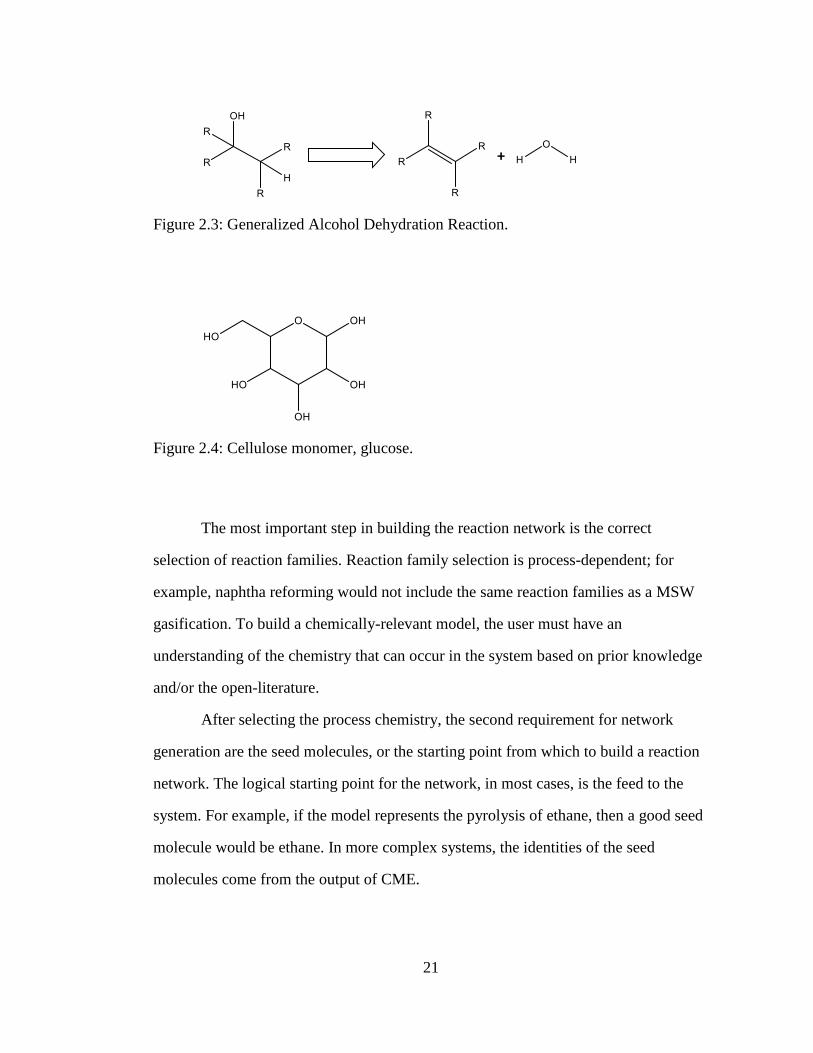
21

Figure 2.3: Generalized Alcohol Dehydration Reaction.

Figure 2.4: Cellulose monomer, glucose.

The most important step in building the reaction network is the correct

selection of reaction families. Reaction family selection is process-dependent; for

example, naphtha reforming would not include the same reaction families as a MSW

gasification. To build a chemically-relevant model, the user must have an

understanding of the chemistry that can occur in the system based on prior knowledge

and/or the open-literature.

After selecting the process chemistry, the second requirement for network

generation are the seed molecules, or the starting point from which to build a reaction

network. The logical starting point for the network, in most cases, is the feed to the

system. For example, if the model represents the pyrolysis of ethane, then a good seed

molecule would be ethane. In more complex systems, the identities of the seed

molecules come from the output of CME.

22

Network generation is an iterative process of finding reactive sites and adding

to the reaction list. The species list begins as the set of seed molecules. Generation

proceeds by searching the first seed molecule and writing all reactions that can occur.

Next, the products of these reactions are checked for any new species. These new

species are added to the species list. Network generation continues through the list of

seeds and product molecules, each time searching for sites and adding valid reactions.

When the end of the species list is reached, all products of all reactions have been

searched for reactive sites. This process has been automated using INGen which has

been developed over many years of research.

2.3.2 History of Reaction Network Generation in KMT

In the Klein research group, automatic generation of molecular-level reaction

networks was originally a tool called NetGen, or Network Generator. This tool was

originally developed by Linda Broadbelt and Scott Stark[38]. NetGen laid out the

groundwork in terms of the representation of molecules and reactions computationally.

At this stage, many features such as reaction types were hard-coded. As such, each

project required expertise in computer science and a deep understanding of the

NetGen tool.

INGen, written by Craig Bennett[44], is the current network-generating

software in KMT. While it is fundamentally based on NetGen, it has many

improvements in terms of the user-interface, the list of pre-made reaction chemistries,

and the simplicity of adding new chemistry. The user-interface is a simple, easy-to-use

Excel interface written in VBA (Visual Basic for the Excel Application). This

interface communicates/runs the back-end program (written in C), which is the

23

workhorse behind network creation. This communication allows a user with minimal

programming experience to build reaction networks.

The interface also allows the user to select reaction chemistries, set reaction

rules (e.g., max carbon number), and select seed molecules from which to begin

network creation. Because of the sheer magnitude of pre-built reaction chemistries,

many kinetic models can be constructed using INGen without program modifications.

Table 2.1 shows the reaction families currently in INGen. Many of the hydrocarbon,

radical, and ion chemistries were added by Bennett in his doctoral thesis. More

recently, the work of Brian Moreno on biomass pyrolysis greatly expanded INGen’s

capabilities by adding new hydrocarbon, nitrogen, sulfur, and radical reaction families.

Most significantly, this work added oxygen chemistry.

INGen contains reaction families at both the mechanistic and pathways levels.

Mechanistic reaction families involve reactive intermediates. In comparison, the

pathways-level reaction families are based on implied mechanisms, such that the steps

involving immeasurable reactive intermediates are lumped into the overall pathway.

Depending on the desired complexity of the reaction network, the user can select

mechanistic or pathways reaction families. Despite the long list of reaction families,

new kinetic models sometimes require the addition of new chemistries. INGen has

streamlined the process of this addition; an expert user can add a new reaction family

in a matter of a few hours.

24

Table 2.1: Reaction families added by Bennett[44] and Moreno[45] to INGen.

Hydrocarbon Methyl Shift Keto-Enol Taut.

Paraffin Methyl Shift β-scission Enol-Keto Taut.

Path A Par. Methyl Shift Hydrogen Abstraction Alkyl Oxidation

Path B1 Par. Methyl Shift Protonation/Deprotonation Aldehyde Oxidation

Path B2 Par. Methyl Shift 5-Member Ring Closure Alcohol Oxidation

Path C Par. Methyl Shift Ring Expansion Hydroperoxide Rearr.

Olefin Methyl Shift Addition Pyran Ring Saturation

Path A Olefin Methyl Shift

Furan Ring Saturation 4H

Path B1 Ole. Methyl Shift Sulfur Decarbonylation

Path B2 Ole. Methyl Shift Desulfonation Decarboxylation

Path C Olefin Methyl Shift Thiopyran Ring Sat. Depolymerization

Aromatic Methyl Shift Thiophene Ring Sat. 2H Hydrolysis

Acyclic Thermal Cracking Thiophene Ring Sat. 4H Ester Hydrolysis

Cyclic Thermal Cracking Hydrodesulfurization Olefin Hydration

Hydrogenation Sulfur Saturation Aldehyde Hydration

Double Bond Shift

Ketone Hydration

Isomerization Oxygen O-O Hydrogenolysis

Cyclization Oxide Thermal Cracking C-O Hydrogenolysis

Hydrogenolysis Retro-Aldol Condensation C-O Hydrogenolysis 5

Cracking Aldol Condensation C-O Hydrogenolysis 6

Dehydrogenation Alcohol Condensation C-O Hydrogenolysis 7

Peracid Condensation Aldehyde Cycl. 5

Nitrogen Water Gas Shift Aldehyde Cycl. 6

Pyrrole Ring Sat. 2H Hydroxyl Shift Ketone Cyclization 5

Pyrrole Ring Sat.4H Alcohol Dehydration Ketone Cyclization 6

Pyridine Ring Sat. 2H Pinacol Rearrangement Carboxyl Cycl. 5

Pyridine Ring Sat. 6H Ortho Acid Dehydration Carboxyl Cycl. 6

Denitrogenation Alcohol Dehydrogenation Alcohol Cyclization 5

Primary Alcohol Dehydro. Alcohol Cyclization 6

Radical Secondary Alcohol Dehydro. Alcohol Cyclization 7

CX Bond Fission Carbonyl Hydrogenation Alcohol Ring Closure 5

HX Bond Fission Aldehyde Hydrogenation Alcohol Ring Closure 7

OX Bond Fission Ketone Hydrogenation O Ring Isomerization

Rad Beta-Scission Carboxyl Hydrogenation Esterification

Rad H-Abstraction Ester Hydrogenation Transesterification

Rad Oxidation Lactone Hydrogenation

Tautomerization

Ion Alde-Enol Tautomerization

Hydride Shift Enol-Alde Tautomerization

25

2.3.2.1 Computational Representation of Reactions

In building reaction networks, INGen represents reactions on a computer. As in

CME, the molecules in INGen are represented using bond-electron matrices.

Reactions extend the matrix analogy and are simply matrix transformations. For

example, the alcohol dehydration of propan-1-ol is given in Figure 2.5. In this

representation, the conversion of reactant to product molecules is governed by the

alcohol dehydration reaction matrix. This matrix and the matrix operation is shown in

Figure 2.6. First, the reduced reactant matrix are atoms whose connectivities will

change in the reaction. The reaction matrix defines how the atomic connectivities

change in the reaction. All reactions within a given reaction family have the same

reaction matrix. Finally, the updated values are represented in the reduced product

matrix. A key concept is that all reactions in the reaction family have the same

reduced reactant matrix, reaction matrix, and reduced product matrix. The reduced

product matrix is used to update the full product matrix as shown in Figure 2.7. In this

case, the full product matrix is split into two separate molecules.

→

+

Reactant Bond

Electron Matrix

Alcohol Dehydration

Reaction Matrix

Product Bond Electron

Matrices

Figure 2.5: alcohol dehydration of propan-1-ol to propene and water.

26

O1 C1 C2 H4

O1 0 1 0 0

C1 1 0 1 0

C2 0 1 0 1

H4 0 0 1 0

+

O1 C1 C2 H4

O1 0 -1 0 1

C1 -1 0 1 0

C2 0 1 0 -1

H4 1 0 -1 0

=

O1 C1 C2 H4

O1 0 0 0 1

C1 0 0 2 0

C2 0 2 0 0

H4 1 0 0 0

Reduced Reactant Matrix Reaction Matrix Reduced Product Matrix

Figure 2.6: Chemical reaction as a matrix operation for propan-1-ol dehydration.

Figure from source material[45].

O1 C1 C2 H4 C3 H1 H2 H3 H5 H6 H7 H8

O1 0 0 0 1 0 1 0 0 0 0 0 0

C1 0 0 2 0 0 0 1 1 0 0 0 0

C2 0 2 0 0 1 0 0 0 1 0 0 0

H4 1 0 0 0 0 0 0 0 0 0 0 0

C3 0 0 1 0 0 0 0 0 0 1 1 1

H1 1 0 0 0 0 0 0 0 0 0 0 0

H2 0 1 0 0 0 0 0 0 0 0 0 0

H3 0 1 0 0 0 0 0 0 0 0 0 0

H5 0 0 1 0 0 0 0 0 0 0 0 0

H6 0 0 0 0 1 0 0 0 0 0 0 0

H7 0 0 0 0 1 0 0 0 0 0 0 0

H8 0 0 0 0 1 0 0 0 0 0 0 0

→

C1 C2 C3 H2 H3 H5 H6 H7 H8

C1 0 2 0 1 1 0 0 0 0

C2 2 0 1 0 0 1 0 0 0

C3 0 1 0 0 0 0 1 1 1

H2 1 0 0 0 0 0 0 0 0

H3 1 0 0 0 0 0 0 0 0

H5 0 1 0 0 0 0 0 0 0

H6 0 0 1 0 0 0 0 0 0

H7 0 0 1 0 0 0 0 0 0

H8 0 0 1 0 0 0 0 0 0

+

O1 H1 H4

O1 0 1 1

H1 1 0 0

H4 1 0 0

Figure 2.7: Separation of the full bond electron matrix post-reaction into product

molecules.

2.4 Equations Written, Solved, and Optimized using the Kinetic Model Editor

The Kinetic Model Editor (KME) first defines the remaining terms on the

material balance, and, then, it writes, solves, and optimizes the kinetic model. There

are two remaining groups of terms in the mass balance, reproduced in Equation 2.4.

The first set of terms is a function of reactor type and represents inlet flows and the

form of the differential equation. The second term represents the reaction rates,

determined by rate laws and underlying rate constants. To write the equations, KME

first utilizes the reaction network produced by INGen. After the equations are written,

27

solution proceeds as an initial value problem where the feed composition is provided

by CME. Finally, KME optimizes rate parameters by comparing model results with

experimental data.

𝑑𝑦




(2.4)

2.4.1 Reactor Type

Reactor type is among the most important design decision in developing a

chemical process model. The type of reactor determines the residence time of

reactants, the effective concentrations of reactants and products, and the temperature

profile in the reactor. Often when modeling a process, idealized reactors are used

individually or in a configuration that mimics the real system. Within KME, the

following reactor types are available: batch reactor, plug-flow reactor (PFR),

continuous stir-tank reactor (CSTR), radial flow reactor (RFR), semibatch reactor,

PFR with sidestream, and continuous catalytic reformer (CCR).

In the material balance equation, reactor type affects the differential term and

the inlet-outlet flows. For example, in a batch reactor, the flow terms are zero and drop

out of the equation. Alternatively, in a PFR, the differential equation is in terms of

reactor length rather than time. The rate expressions are invariant with reactor type,

but reaction rates can be drastically affected as different reactor types affect the

effective concentrations of reactants and products.

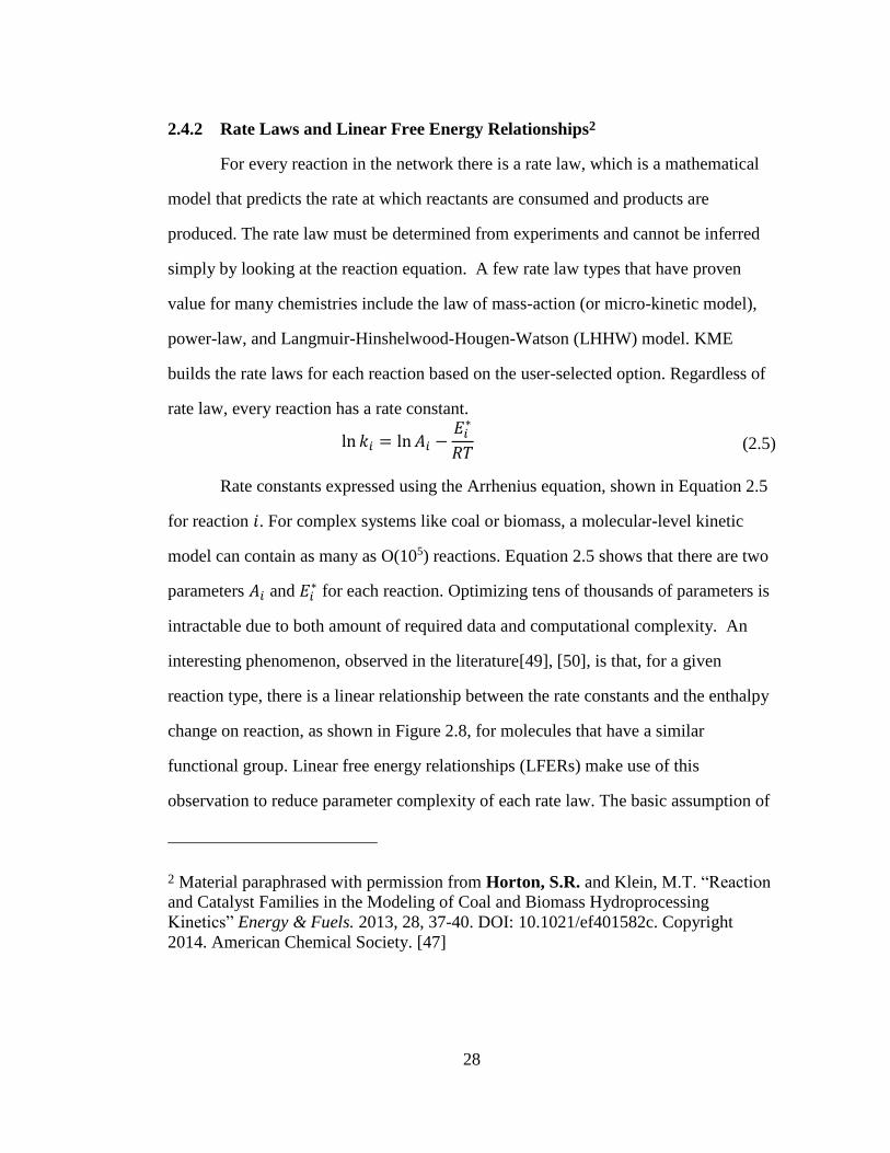
28

2.4.2 Rate Laws and Linear Free Energy Relationships2

For every reaction in the network there is a rate law, which is a mathematical

model that predicts the rate at which reactants are consumed and products are

produced. The rate law must be determined from experiments and cannot be inferred

simply by looking at the reaction equation. A few rate law types that have proven

value for many chemistries include the law of mass-action (or micro-kinetic model),

power-law, and Langmuir-Hinshelwood-Hougen-Watson (LHHW) model. KME

builds the rate laws for each reaction based on the user-selected option. Regardless of

rate law, every reaction has a rate constant.

ln 𝑘𝑖 = ln𝐴𝑖 −𝐸𝑖∗

𝑅𝑇 (2.5)

Rate constants expressed using the Arrhenius equation, shown in Equation 2.5

for reaction 𝑖. For complex systems like coal or biomass, a molecular-level kinetic

model can contain as many as O(105) reactions. Equation 2.5 shows that there are two

parameters 𝐴𝑖 and 𝐸𝑖∗ for each reaction. Optimizing tens of thousands of parameters is

intractable due to both amount of required data and computational complexity. An

interesting phenomenon, observed in the literature[49], [50], is that, for a given

reaction type, there is a linear relationship between the rate constants and the enthalpy

change on reaction, as shown in Figure 2.8, for molecules that have a similar

functional group. Linear free energy relationships (LFERs) make use of this

observation to reduce parameter complexity of each rate law. The basic assumption of

2 Material paraphrased with permission from Horton, S.R. and Klein, M.T. “Reaction

and Catalyst Families in the Modeling of Coal and Biomass Hydroprocessing

Kinetics” Energy & Fuels. 2013, 28, 37-40. DOI: 10.1021/ef401582c. Copyright

2014. American Chemical Society. [47]

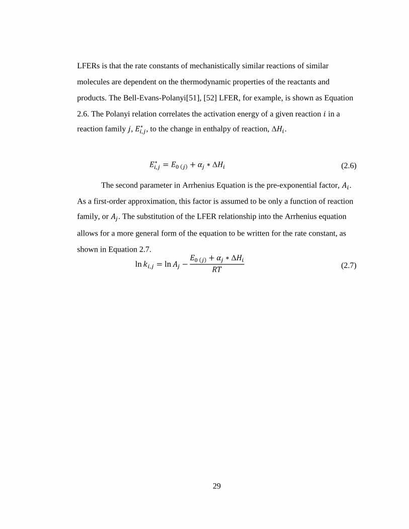
29

LFERs is that the rate constants of mechanistically similar reactions of similar

molecules are dependent on the thermodynamic properties of the reactants and

products. The Bell-Evans-Polanyi[51], [52] LFER, for example, is shown as Equation

2.6. The Polanyi relation correlates the activation energy of a given reaction 𝑖 in a

reaction family 𝑗, 𝐸𝑖,𝑗∗ , to the change in enthalpy of reaction, Δ𝐻𝑖.

𝐸𝑖,𝑗∗ = 𝐸0 (𝑗) + 𝛼𝑗 ∗ Δ𝐻𝑖 (2.6)

The second parameter in Arrhenius Equation is the pre-exponential factor, 𝐴𝑖.

As a first-order approximation, this factor is assumed to be only a function of reaction

family, or 𝐴𝑗. The substitution of the LFER relationship into the Arrhenius equation

allows for a more general form of the equation to be written for the rate constant, as

shown in Equation 2.7.

ln 𝑘𝑖,𝑗 = ln𝐴𝑗 −𝐸0 (𝑗) + 𝛼𝑗 ∗ Δ𝐻𝑖

𝑅𝑇 (2.7)

30

Figure 2.8: Figure from Horton and Klein[47]. (a) Figure reproduced Mochida and

Yoneda[49] showing the dealyklation of alkylaromatics reaction family

on a SA-1-Na-3 catalyst. The numbers represent experimental rates of

dealkylation on different alkyl aromatics.

The major impact of using LFERs for reaction families is the massive

reduction in the number of adjustable parameters in the kinetic model. Relating back

to the original mass balance equation, the adjustable parameters in a molecular-level

kinetic model are within the rate constants for each of the reactions where there are

two rate parameters per rate constant. As it was shown, LFERs reduce the number of

adjustable parameters down to three per reaction family. This drastically reduces the

experimental data and computational time required to optimize a kinetic model.

2.4.3 Model Solution

At this stage, the material balance equations have been completely defined.

KME takes these concepts and automatically writes the material balance differential

equations[2],[3],[42]. Within KME, the differential equation solver suite is the open-

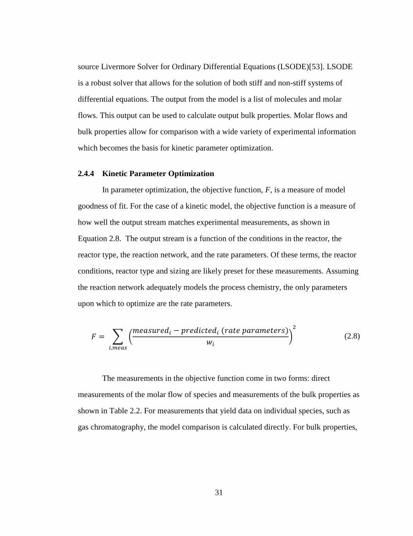
31

source Livermore Solver for Ordinary Differential Equations (LSODE)[53]. LSODE

is a robust solver that allows for the solution of both stiff and non-stiff systems of

differential equations. The output from the model is a list of molecules and molar

flows. This output can be used to calculate output bulk properties. Molar flows and

bulk properties allow for comparison with a wide variety of experimental information

which becomes the basis for kinetic parameter optimization.

2.4.4 Kinetic Parameter Optimization

In parameter optimization, the objective function, F, is a measure of model

goodness of fit. For the case of a kinetic model, the objective function is a measure of

how well the output stream matches experimental measurements, as shown in

Equation 2.8. The output stream is a function of the conditions in the reactor, the

reactor type, the reaction network, and the rate parameters. Of these terms, the reactor

conditions, reactor type and sizing are likely preset for these measurements. Assuming

the reaction network adequately models the process chemistry, the only parameters

upon which to optimize are the rate parameters.

𝐹 = ∑ (𝑚𝑒𝑎𝑠𝑢𝑟𝑒𝑑𝑖 − 𝑝𝑟𝑒𝑑𝑖𝑐𝑡𝑒𝑑𝑖 (𝑟𝑎𝑡𝑒 𝑝𝑎𝑟𝑎𝑚𝑒𝑡𝑒𝑟𝑠)

𝑤𝑖)2

𝑖,𝑚𝑒𝑎𝑠

(2.8)

The measurements in the objective function come in two forms: direct

measurements of the molar flow of species and measurements of the bulk properties as

shown in Table 2.2. For measurements that yield data on individual species, such as

gas chromatography, the model comparison is calculated directly. For bulk properties,

32

the comparison is made implicitly by converting the product composition to predicted

properties via structure property correlations.

Table 2.2: The two types of measurements in the objective function.

Overall

Objective

Function

𝑀𝑜𝑙𝑎𝑟 𝐹𝑙𝑜𝑤 𝑇𝑒𝑟𝑚𝑠 + 𝐵𝑢𝑙𝑘 𝑃𝑟𝑜𝑝𝑒𝑟𝑡𝑦 𝑇𝑒𝑟𝑚𝑠

Molar

Flow

Terms

∑ ((𝑚𝑒𝑎𝑠𝑢𝑟𝑒𝑑 𝑓𝑙𝑜𝑤)𝑖 − (𝑝𝑟𝑒𝑑𝑖𝑐𝑡𝑒𝑑 𝑓𝑙𝑜𝑤)𝑖

𝑤𝑖)

2

𝑖, 𝑠𝑝𝑒𝑐𝑖𝑒𝑠

Bulk

Property

Terms

∑ ((𝑚𝑒𝑎𝑠𝑢𝑟𝑒𝑑 𝑝𝑟𝑜𝑝𝑒𝑟𝑡𝑦)𝑖 − (𝑝𝑟𝑒𝑑𝑖𝑐𝑡𝑒𝑑 𝑝𝑟𝑜𝑝𝑒𝑟𝑡𝑦)𝑖

𝑤𝑖)

2

𝑖, 𝑝𝑟𝑜𝑝𝑒𝑟𝑡𝑖𝑒𝑠

Using the objective function, KME optimizes the model to experimental data.

The major optimization routine is simulated annealing, a global optimization

algorithm. Global optimization techniques are specifically designed to find the global

minimum in a problem with a high number of parameters. Most global optimization

algorithms rely on randomly sampling new parameter values from the range of

allowable parameter values. Another characteristic of global optimizers is that they

have some probability of allowing uphill steps, or steps that increase the value of the

objective function. This may seem counter-intuitive, but it is this characteristic which

allows the solution to escape local minima. Global optimizers are the only feasible

way to solve high-parameter optimization problems.

Once the numerical optimizer reaches a satisfactory objective function value,

the result is a list of tuned kinetic parameters and the corresponding comparison of

predicted to measured experimental results. A common plot drawn to analyze the fit of

these results is a parity plot as shown in Figure 2.9. In parity plots, the model

33

predictions are on the y-axis, and experimental measurements are on the x-axis. The

line y=x corresponds then to a perfect model prediction.

Figure 2.9: Example parity plot for the pyrolysis of naphtha for an experimental

carbon number distribution. Figure from source material[42].

2.5 Summary

In summary, a molecular-level kinetic model is fundamentally a system of

material balance differential equations with one equation per species. The three

software tools that make up KMT each build different terms in the differential

equations. CME finds the initial value of the system by finding the optimal feed

composition for a set of experimental measurements. INGen builds a reaction network

by utilizing the feed composition and an understanding of process chemistry. With this

reaction network, KME writes the material balances using user-defined rate laws and

reactor types. After constructing the system of equations, KME solves the reactor

model. The adjustable parameters are reaction family LFER parameters. Comparison

34

with experimental measurements allows for an optimization of the kinetic parameters.

The results from optimization are a set of tuned LFER parameters. The optimization

results can be analyzed using a parity plot showing model predictions and

experimental measurements.

35

MOLECULAR-LEVEL KINETIC MODELING OF THE GASIFICATION OF

COMMON PLASTICS

Scott R. Horton1, James Woeckener1, Rebecca Mohr2, Yu Zhang2, Francis Petrocelli2, and Michael T. Klein1

1University of Delaware Energy Institute and Department of Chemical and

Biomolecular Engineering, University of Delaware, Newark, DE 19716 2Air Products and Chemicals Incorporated. Allentown, PA, 18195

Reproduced by permission from Horton, S.R.; Woeckener, J.; Mohr, R.; Zhang, Y.;

Petrocelli, F.; Klein, M.T. “Molecular-level kinetic modeling of the gasification of

common plastics.” Energy & Fuels. 2015 (Web).

DOI:10.1021/acs.energyfuels.5b02047. Copyright 2015. American Chemical

Society.[54]

Chapter 3

36

3.1 Abstract

A molecular-level kinetic model was developed for the gasification of common

plastics including poly-ethylene (PE), polyethylene terephthalate (PET), polyvinyl

chloride (PVC), and polystyrene (PS). Model development was divided into three

steps: molecular characterization of the feed, generation of a pathways-level reaction

network, and creation of the material balance differential equations (DEs). The

structure of all polymers was modeled as linear with known repeat units. For PE, PVC,

and PET Flory-Stockmayer statistics were used to describe the initial polymer size

distribution; PS was described using a two-parameter gamma distribution. The

parameters of all polymer size distributions were tuned using data from the open

literature.

The chemistry of plastics gasification contains depolymerization, pyrolysis,

and gasification reactions. The initial depolymerization of PE and PET was modeled

using random scission and Flory-Stockmayer statistics. A statistical method was

created extending random scission to a generalized polymer size distribution and

applied here to the breakdown of polystyrene. The depolymerization of PVC was

modeled as two-step: poly-ene formation followed by benzene production. Pyrolysis

reactions were included on small oligomers and were broken down into two

categories: cracking and formation of tar and char molecules. For gasification,

incomplete combustion and steam reforming were included to break down oligomers,

tar, and char molecules. Also, light gas reactions, e.g., water-gas shift, were added to

the network. The final network contained 283 reactions and 85 species.

After construction of the material balance DEs, kinetic parameters were tuned

using literature data on each plastic. These studies involved gasification, pyrolysis,

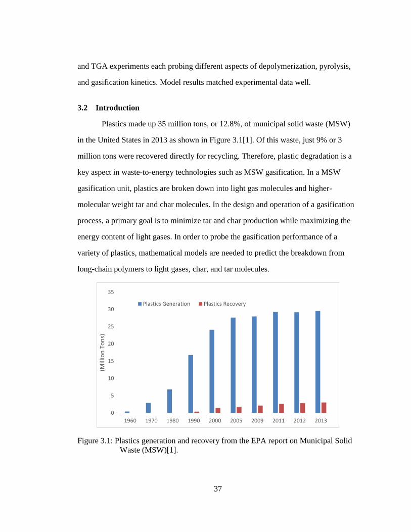
37

and TGA experiments each probing different aspects of depolymerization, pyrolysis,

and gasification kinetics. Model results matched experimental data well.

3.2 Introduction

Plastics made up 35 million tons, or 12.8%, of municipal solid waste (MSW)

in the United States in 2013 as shown in Figure 3.1[1]. Of this waste, just 9% or 3

million tons were recovered directly for recycling. Therefore, plastic degradation is a

key aspect in waste-to-energy technologies such as MSW gasification. In a MSW

gasification unit, plastics are broken down into light gas molecules and higher-

molecular weight tar and char molecules. In the design and operation of a gasification

process, a primary goal is to minimize tar and char production while maximizing the

energy content of light gases. In order to probe the gasification performance of a

variety of plastics, mathematical models are needed to predict the breakdown from

long-chain polymers to light gases, char, and tar molecules.

Figure 3.1: Plastics generation and recovery from the EPA report on Municipal Solid

Waste (MSW)[1].

0

5

10

15

20

25

30

35

1960 1970 1980 1990 2000 2005 2009 2011 2012 2013

(Mill

ion

To

ns)

Plastics Generation Plastics Recovery

38

Prior work in the mathematical modeling of depolymerization of plastics can

be divided into two categories: pyrolysis and gasification. For pyrolysis, there have

been some very detailed studies of chemical kinetics at the radical level for individual

common polymers. For example, polystyrene has been studied extensively by

Broadbelt and coworkers[55],[56]. Similarly, there is a mechanistic understanding of

the pyrolysis of ethane[57]; which is directly applicable to polyethylene. There has

also been detailed work on the pyrolysis of plastic mixtures[58]. The detail of

mathematical models in the gasification literature is far less prevalent and complex.

Some studies fit lumped kinetic parameters to Thermogravimetric Analysis (TGA)

data[59],[60]; however, complex kinetic models at the molecular-level are missing

from the plastic gasification literature.

The current modeling work is the first representation in the open literature of a

molecular-level kinetic model for the gasification of common plastics; specifically,

PE, PET, PVC, and PS. Modeling kinetics at the molecular-level requires molecular

detail at every step in the model-building process. First, the feed is modeled as a

collection of molecules and mole fractions. Next, the reaction network utilizes

fundamental chemistry to describe the mapping from reactant to product molecules.

This network is used to construct a set of material balance differential equations for

each molecular species. The feed composition specifies the initial values of these

differential equations. The kinetic model can be integrated for a given set of reactor

conditions and reactor type. The adjustable parameters in the model are the kinetic

parameters to each reaction chemistry. Experimental data from the open literature

allows for both kinetic parameter tuning and model evaluation.

39

3.3 Molecular Representation of Plastics

The first step in building a molecular-level kinetic model is the molecular

representation of the feedstock. If the polymers are assumed to be linear, then the

composition is defined by the repeat unit structure and a polymer-size distribution.

The repeat unit structures for the polymers in this study are shown below in Figure

3.2. In this report, the polymers were described using two types of polymer size

distributions. A single-parameter Flory distribution is used for PE, PVC, and PET, and

a two-parameter gamma distribution is used for polystyrene. The adjustable

parameters in the composition model are then the parameters of the distribution; these

parameters were optimized using literature data on each of the polymers.

The molecular structure of a polymer can also be conceptualized as cores with

inter-core linkage (IL) and side chain (SC) substituents. Cores are connected by ILs to

form polymers, and SCs are terminal end groups. For example, in polyethylene, the

core identity is C2H4, the IL is the bond between cores, and a SC is a terminal bond to

hydrogen. Each core has two binding sites for substituents, filled by either ILs or SCs.

Because SCs are terminal, each linear polymer chain only has two SCs. In a linear

polymer, an i-mer contains i cores, i-1 ILs, and 2 SCs.

Figure 3.2: Repeat Unit Structures for PE, PVC, PET, and PS (Left to Right).

40

3.3.1 Flory-distributed Linear Polymers

One of the most commonly used polymer-size distributions is the single-

parameter Flory distribution[61], given in Equation 3.1. The p used in this equation is

commonly the extent of polymerization, and is equivalently the fraction of core

binding sites contained within linkages, given in Equation 3.2. A common measure of

linear polymers is the number average degree of polymerization, 𝑋𝑛̅̅̅̅ , which is

calculated directly from p using Equation 3.3. The composition of a Flory-distributed

linear polymer is therefore defined by repeat unit structure and average degree of

polymerization.

𝑥𝑖 = (1 − 𝑝) ∗ 𝑝𝑖−1 (3.1)

𝑝 =2 ∗ [𝐼𝐿]

2 ∗ [𝐼𝐿] + [𝑆𝐶]

(3.2)

𝑋𝑛̅̅̅̅ =1

1 − 𝑝

(3.3)

For each Flory-distributed linear polymer, literature ultimate analyses were

used to find optimal values of 𝑋𝑛̅̅̅̅ . For these optimizations, an in-house software tool

called Linear Polymer Composition Editor was utilized. Further detail on this tool can

be found in prior work[54]. The results for the composition models are summarized

below in Table 3.1. In these results, PE and PET matched well with experimental

data. The minor discrepancies in polyvinyl chloride could be explained by the

presence of plasticizers, a common PVC additive[62], in the experimental sample that

are absent in the composition model. The role of these plasticizers in the composition

and subsequent kinetic model is assumed to be a second-order effect, but is an

opportunity for future work. Although more detailed distribution information, such as

polydispersity index (PDI), was not measured experimentally, the agreement with

41

available data suggests the Flory distribution is applicable to PE, PET, and PVC in the

composition model.

Table 3.1: Experimental and predicted ultimate analyses for PE, PVC, and PET. The

literature values are from Arena et al.[23] for PE, Heikkinen et al[63] for

PET, and Zhu et al. for PVC[64]. The 𝑋𝑛̅̅̅̅ ′𝑠 for these results are 291, 998,

and 5 for PE, PET, and PVC respectively.

Element Polyethylene Polyethylene Terephthalate

Polyvinyl Chloride

Experimental Predicted Exp. Pred. Exp. Pred. C 85.0 85.6 62.51 62.49 41.55 38.1 H 13.8 14.4 4.19 4.20 4.81 5.44 O 0.00 0.00 33.30 33.3 0.00 0.00 Cl 0.00 0.00 0.00 0.00 52.95 56.38

The Flory distribution is not well-suited as a composition model for all

polymers; this is exemplified by polystyrene. At the lab scale, polystyrene is often

synthesized via anionic polymerization with typical PDI values of 1.05[65], [66].

These samples were found to behave similarly to commercial polystyrene under

pyrolysis conditions[65]. At long chains, the Flory distribution converges on a

polydispersity index (PDI) of 2.00. Due to the discrepancy in PDI, polystyrene was

instead modeled using a 2-parameter gamma distribution.

3.3.2 Gamma-distributed Linear Polymers

The two-parameter gamma distribution is given in Equation 3.4 where a and d

are shape and scale factors, respectively. Experimental measurements were used to

optimize the parameters for the distribution. In this case, the data for polystyrene are

the number average molecular weight, 𝑀𝑛̅̅ ̅̅ , and weight average molecular weight,

𝑀𝑤̅̅ ̅̅̅. After finding optimal gamma parameters, a comparison of experimental results

42

and predictions are given below in Table 3.2. The results fit the data well suggesting

that the gamma distribution is appropriate for polystyrene.

𝑥𝑖(𝑎, 𝑑) =𝑖𝑑−1 ∗ 𝑒−

𝑖𝑎

𝑎𝑑 ∗ Γ(𝑑)

(3.4)

Table 3.2: Literature measurements for polystyrene and corresponding gamma

predictions. 𝑀𝑤̅̅ ̅̅̅ was reported in Liu et al[67], approximate literature PDI

values were used to approximate 𝑀𝑛̅̅ ̅̅ . The gamma parameters for these

values were calculated to be: 𝑎 = 13037.43, 𝑑 = 20.

3.4 Reaction Chemistry of Gasification of Plastics

The second step of building a molecular-level kinetic model is the generation

of the reaction network. This network contains the fundamental process chemistry for

the gasification of plastics. In this model, first the long-chain polymers are

depolymerized into smaller oligomers via depolymerization reactions. The small

oligomers then react further via more detailed pyrolysis and gasification chemistry to

form light gas, tar, and char molecules.

3.4.1 Depolymerization

Depolymerization chemistry breaks down the initial polymer backbone.

Although these chemistries are polymer specific, there are common types of

Parameter Experimental

Value

Value from

Gamma

Distribution

𝑴𝒏̅̅ ̅̅ (

𝒈

𝒎𝒐𝒍) 260749 260637

𝑴𝒘̅̅ ̅̅ ̅ (

𝒈

𝒎𝒐𝒍) 273786 273571

𝑷𝑫𝑰 = 𝟏. 𝟎𝟓 1.05 1.049

43

depolymerization. For example, many mechanisms occur randomly along the polymer

backbone and are known as random scission mechanisms. Due to the random nature of

the mechanism, it is possible to predict the changes in the polymer size distribution

over the course of depolymerization. This allows the model to account for large mers

without the unnecessary computational burden of individually tracking hundreds to

thousands of mers over the course of depolymerization.

3.4.1.1 Random Scission of Flory Polymers

Random scission depolymerization is most easily applied to Flory polymers. In

polymerization, the Flory distribution assumes that all end-groups are equally reactive

and therefore linkages are randomly formed in the system. Random scission is simply

the reverse of this process, and the Flory distribution, given before in Equation 3.1,

still applies to the product polymer. Because the distribution is still applicable,

depolymerization simply decreases the value of p.

Depolymerization can also be related to the concept of cores, ILs, and SCs. If

depolymerization is represented using a single link cleavage reaction in Equation 3.5,

then the change of ILs in the system can be related to the Flory parameter as shown in

Equation 3.6. The constant, C, follows from the link cleavage reaction and represents

the number of substituent sites in the system.

𝐼𝐿 → 𝑆𝐶0 + 𝑆𝐶1 (3.5)

𝑑𝑝

𝑑𝑡=2

𝐶∗𝑑[𝐼𝐿]

𝑑𝑡, 𝐶 = 2 ∗ [𝐼𝐿] + [𝑆𝐶]

(3.6)

As described previously, this statistical description is utilized only for the

initial breakdown, and more detailed pyrolysis and gasification chemistry will be

utilized on small oligomers. The output from the statistical method, 𝑑[𝐼𝐿]

𝑑𝑡, must

therefore supply the input to the explicit material balances for the oligomers in the

44

molecular model. The Flory distribution is scaled such that the boundary oligomers

occur at i=1. This effectively transforms the 1-mer from a monomer to an oligomer in

the distribution. The oligomer molar flow rate is then given in Equation 3.7 and

represented by 𝑁1. Equation 3.8 gives the increase in 𝑁1 from depolymerization.

𝑁1 =𝐶

2∗ (1 − 𝑝)2

(3.7)

𝑑𝑁1𝑑𝑡

=𝐶

2∗ −2 ∗ (1 − 𝑝) ∗

𝑑𝑝

𝑑𝑡= −2 ∗ (1 − 𝑝) ∗

𝑑[𝐼𝐿]

𝑑𝑡

(3.8)

3.4.1.2 Random Scission Method for a Generalized Polymer Size Distribution

For polymers modeled using more complex polymer size distributions, the

random scission method is not as easily applied. For instance, in this work,

polystyrene was represented using a gamma distribution. Rather than utilizing a

method specific to gamma distributions, the far more interesting derivation is for a

generalized polymer-size distribution. In the general case, consider the polymer size

distribution as a histogram, as illustrated in Figure 3.3, where the mole fraction of

every mer is independent. The goal, as before, is to correlate the changes in linkage

concentration to the changes in molar flow rates of mers in the system. This allows for

a prediction of the histogram after depolymerization.

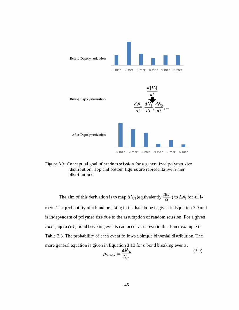
45

Before Depolymerization

During Depolymerization

𝑑[𝐼𝐿]

𝑑𝑡

𝑑𝑁1𝑑𝑡,𝑑𝑁2𝑑𝑡,𝑑𝑁3𝑑𝑡, …

After Depolymerization

Figure 3.3: Conceptual goal of random scission for a generalized polymer size

distribution. Top and bottom figures are representative n-mer

distributions.

The aim of this derivation is to map Δ𝑁𝐼𝐿(equivalently 𝑑[𝐼𝐿]

𝑑𝑡 ) to Δ𝑁𝑖 for all i-

mers. The probability of a bond breaking in the backbone is given in Equation 3.9 and

is independent of polymer size due to the assumption of random scission. For a given

i-mer, up to (i-1) bond breaking events can occur as shown in the 4-mer example in

Table 3.3. The probability of each event follows a simple binomial distribution. The

more general equation is given in Equation 3.10 for n bond breaking events.

𝑝𝑏𝑟𝑒𝑎𝑘 =Δ𝑁𝐼𝐿𝑁𝐼𝐿

(3.9)

1-mer 2-mer 3-mer 4-mer 5-mer 6-mer

1-mer 2-mer 3-mer 4-mer 5-mer 6-mer

46

𝑝𝑏𝑛 = (1 − 𝑝𝑏𝑟𝑒𝑎𝑘)𝑖−1−𝑛 ∗ 𝑝𝑏𝑟𝑒𝑎𝑘

𝑛 ∗ (𝑖 − 1𝑛) (3.10)

Table 3.3: Probability of bonds broken within a 4-mer.

Bonds Broken Probability

0 𝑝𝑏0 = (1 − 𝑝𝑏𝑟𝑒𝑎𝑘)3 ∗ (

30)

1 𝑝𝑏1 = (1 − 𝑝𝑏𝑟𝑒𝑎𝑘)2 ∗ 𝑝𝑏𝑟𝑒𝑎𝑘

∗ (31)

2 𝑝𝑏2 = (1 − 𝑝𝑏𝑟𝑒𝑎𝑘) ∗ 𝑝𝑏𝑟𝑒𝑎𝑘2 ∗ (

32)

3 𝑝𝑏3 = 𝑝𝑏𝑟𝑒𝑎𝑘3 ∗ (

33)

After calculating the probability of bond breaking events in an i-mer, the next

step is to calculate the amount of smaller mer production. For example, 4-mer

breakdown is shown in Figure 3.4. If a single bond breaking event occurs in a 4-mer,

there are three possible bonds to break. Two of the three bonds produce a trimer and a

monomer, and the other bond produces 2 dimers. The expected production from one

bond breaking event is therefore 2

3 of each smaller mer. This method is extended to

multiple bond breaking events. The breakdown matrix format is easier to visualize,

each row corresponds to a bond breaking event. The columns correspond to the

relative amounts of each j-mer produced by that specific event.

47

Each i-mer has its own unique breakdown matrix; however, all breakdown

matrices can be filled using a generalized formula, given in Equation 3.11. The terms

of this equation are described using Table 3.4. The general logic is that each row in the

matrix is filled sequentially. The first row is known, if zero bond breaking events

occur, then the i-mer remains unreacted. For subsequent rows, each column (j-mer) is

calculated using a standard balance format: (value from previous bond breaking event)

– (consumption in this bond breaking event) + (production in this bond breaking

event).

𝑚𝑛+1,𝑗 = 𝑚𝑛,𝑗 −𝑚𝑛,𝑗 ∗𝑗 − 1

𝑖 − 𝑗+ ∑ 𝑚𝑛,𝑘 ∗

𝑘 − 1

𝑖 − 𝑛∗ (

2

𝑘 − 1)

𝑖−𝑛+1

𝑘=𝑗+1

(3.11)

1-mer 2-mer 3-mer 4-mer

𝑝𝑏0 0 0 0 1

𝑝𝑏1 2

3

2

3

2

3 0

𝑝𝑏2 2 1 0 0

𝑝𝑏3 4 0 0 0

Figure 3.4: Illustration (top) and breakdown matrix representation (bottom)

of possible bond breaking events in a 4-mer. Values in the

matrix are relative initial amount of 4-mer.

48

Table 3.4: Description of terms Equation 3.11. The notation is 𝑚𝑟𝑜𝑤,𝑐𝑜𝑙𝑢𝑚𝑛 for the

breakdown matrix. The row corresponds to total number of bonds

breaking in the i-mer. The column corresponds to the production of

smaller j-mers from the breakdown of i-mer.

Term Description 𝒎𝒏+𝟏,𝒋 Breakdown matrix

value for row (n+1), column j.

𝒎𝒏,𝒋 Value from the previous break for j-mer.

𝒎𝒏,𝒋 ∗𝒋 − 𝟏

𝒊 − 𝒋

Amount of j-mer breaking down in this bond breaking event

∑ 𝒎𝒏,𝒌 ∗𝒌 − 𝟏

𝒊 − 𝒏∗ (

𝟐

𝒌 − 𝟏)

𝒊−𝒏+𝟏

𝒌=𝒋+𝟏

j-mer production from larger k-mers

With the breakdown matrices filled for all i-mers, the remaining step is to

calculate the new values for molar flow rates of each i-mer, 𝑁𝑖,𝑛𝑒𝑤. The formula, given

by Equation 3.12, simply loops over all larger mers and utilizes the values from the

breakdown matrices to calculate the new flow rate. This result gives the complete

updated histogram for a change in IL concentration.

𝑁𝑖,𝑛𝑒𝑤 = ∑ 𝑁𝑗,𝑜𝑙𝑑

𝑚𝑎𝑥

𝑗=𝑖

∗(∑ 𝑝𝑏𝑘 ∗ (𝑚𝑘,𝑖)

(𝑗−1)

𝑘=0

) ,𝑤ℎ𝑒𝑟𝑒 𝑚𝑎𝑥 𝑖𝑠 𝑡ℎ𝑒 𝑙𝑎𝑟𝑔𝑒𝑠𝑡 𝑚𝑒𝑟

(3.12)

In order to address numerical issues with large n-mers, two simplifications can

be made in the use of this algorithm. Because this method is used in conjunction with

a system of differential equations, Δ𝐼𝐿 in any given time step is small. This allows for

the simplification that only a few bond breaking events occur in any given reaction

49

step. This reduces the numerical complexity that arises in the combinatorial term in

the binomial calculation in Equation 3.10. The second simplification is to lump

similarly-sized mers. For example, if histogram only tracks every 20-mers, then much

longer mers can be calculated quickly while only losing the more minute detail.

3.4.1.3 Depolymerization Chemistry – PE

The thermal depolymerization of polyethylene proceeds via a radical cracking

mechanism[68] containing two primary mechanistic steps: H-abstraction and 𝛽-

scission, shown in Figure 3.5. The products from depolymerization arise from relative

stabilities of radicals. For instance, after a cracking reaction, the instability of the

primary product radical means unzipping is unlikely to occur, and monomer yield is

low[68]. Instead, the product from 𝛽-scission is likely to abstract a hydrogen either

intramolecularly or intermolecularly. In the intramolecular case, H-abstraction occurs

on the same chain, likely at the 6-carbon location due to a 6-member ring transition

state[69]; this step is often called backbiting. If H-abstraction occurs intermolecularly,

then the depolymerization has random-scission type behavior. In order to

accommodate both mechanisms, the initial breakdown was performed using random

scission, and 3-mer was selected as the largest oligomer for full pyrolytic detail. H-abstraction

β-Scission

Figure 3.5: Radical propagation steps for polyethylene depolymerization. The H-

abstraction step shown here is inter-molecular and can occur with any

radical in the system.

50

There are three possible 6-carbon oligomers from the thermal cracking of

polyethylene: hexane, hex-1-ene, and hexa-1,5-diene shown in Figure 3.6. In this

mechanism, each bond breaking event produces one double bond end group and one

single bond end group. It therefore follows that there should be approximately a 1:2:1

ratio of these products. If the assumption is made that all initial end groups are

saturated, then the ratio is slightly skewed toward hexane. During depolymerization,

the link cleavage reaction in Equation 3.5 keeps track of the relative amounts of single

bond and double bond end groups. This allows for the ratio of 6-carbon oligomers to

be calculated at any time.

Figure 3.6: Oligomers with 6-carbons produced during polyethylene

depolymerization. These are the starting molecules from polyethylene for

the full pyrolysis and gasification network.

3.4.1.4 Depolymerization Chemistry – PET

The thermal depolymerization of PET follows the mechanism[70],[71] shown

in Figure 3.7. Because this mechanism is concerted and thermal, the random scission

assumption applies. For PET, a dimer was chosen as the oligomer size for more

detailed chemistry. This allowed the inclusion of a charring mechanism to occur on

the PET linkage as will be shown later when discussing pyrolysis. Again, there are

three possible 2-mers based on the different combinations of end groups.

51

Figure 3.7: Link cleavage in polyethylene terephthalate (concerted mechanism).

3.4.1.5 Depolymerization Chemistry – PVC

The depolymerization of polyvinylchloride is modeled as a two-step

depolymerization given in Figure 3.8. The first step, dehydrochlorination, occurs very

quickly producing HCl and a poly-ene structure[68], [72]. The second step of PVC

breakdown is less well understood and far slower. Benzene is one of the most common

volatile products from thermal breakdown[73]. To account for benzene production, a

pinch-off mechanism[72] was utilized to further breakdown the polyene structure.

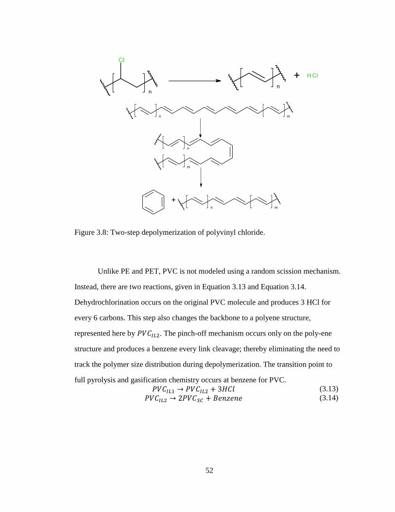
52

Figure 3.8: Two-step depolymerization of polyvinyl chloride.

Unlike PE and PET, PVC is not modeled using a random scission mechanism.

Instead, there are two reactions, given in Equation 3.13 and Equation 3.14.

Dehydrochlorination occurs on the original PVC molecule and produces 3 HCl for

every 6 carbons. This step also changes the backbone to a polyene structure,

represented here by 𝑃𝑉𝐶𝐼𝐿2. The pinch-off mechanism occurs only on the poly-ene

structure and produces a benzene every link cleavage; thereby eliminating the need to

track the polymer size distribution during depolymerization. The transition point to

full pyrolysis and gasification chemistry occurs at benzene for PVC.

𝑃𝑉𝐶𝐼𝐿1 → 𝑃𝑉𝐶𝐼𝐿2 + 3𝐻𝐶𝑙 (3.13)

𝑃𝑉𝐶𝐼𝐿2 → 2𝑃𝑉𝐶𝑆𝐶 + 𝐵𝑒𝑛𝑧𝑒𝑛𝑒 (3.14)

53

3.4.1.6 Depolymerization Chemistry – PS

The depolymerization of polystyrene is a radical cracking mechanism.

Differences between the polymers is due to the stability of the radicals shown in Table

3.5. Unlike polyethylene, the end-group radical is a benzylic radical and is stable

allowing for unzipping-type mechanisms to occur. Also, there are two stable

intramolecular H-abstraction reactions leading to backbiting and production of dimers

and trimers. Finally, as before, intermolecular H-abstraction can occur in a random-

scission type mechanism. All of these mechanisms were included in the

depolymerization model.

A multi-step breakdown method was used for polystyrene depolymerization.

For the initial breakdown from large n-mer, random scission for a generalized polymer

size distribution was utilized with 20-mer lumps. For 20-mer and smaller, a standard

population balance was used with a differential equation for every mer.

Depolymerization reactions for all four mechanisms from Table 3.5 were included on

these mers. Finally, for styrene monomers, full pyrolysis and gasification chemistry

was allowed to break down the structure into light gases.

54

Table 3.5: Stable radicals and products from included mechanisms in polystyrene

degradation.

Type Stable Radical Products

Unzipping

Dimer Backbiting

Trimer Backbiting

Random Scission

Spectrum of mono- and di-olefin n-mers

3.4.2 Pyrolysis of Oligomers

Pyrolysis chemistry occurs without the presence of reactive gases. In the case

of plastics, there are two general types of pyrolysis reactions: cracking reactions which

serve to break down molecules and charring reactions which serve to build up stable

higher-MW species. In this network, the dominant cracking reaction families were

acyclic thermal cracking, decarboxylation, and decarbonylation given in Table 3.6.

These reaction families are well known and have been used in previous models[74].

Less common cracking mechanisms, ester decarboxylation and rearrangement, were

proposed in the PET pyrolysis literature[75], and were included in this model.

55

Table 3.6: Pyrolysis cracking reaction families, reaction matrices, and example

reactions. The reaction matrix contains -1 for bond-breaking and -1 for

bond-making during reaction.

Reaction Type (Family) and Reactive Moetiy

Reaction Matrix Example Reaction

Decarbonylation Aldehydes

H O C R

H 0 0 -1 1

O 0 0 1 0

C -1 1 0 -1

R 1 0 -1 0

Decarboxylation Carboxylic acids

H O C R

H 0 -1 0 1

O -1 0 1 0

C 0 1 0 -1

R 1 0 -1 0

Acyclic Thermal Cracking Hydrocarbon side chains and irreducible molecules

C C C H

C 0 -1 0 1

C -1 0 1 0

C 0 1 0 -1

H 1 0 -1 0

Ester Decarboxylation Esters

H O C C

H 0 -1 0 1

O -1 0 1 0

C 0 1 0 -1

C 1 0 -1 0

Ester Rearrangement Esters adjacent to a double bond

H O C C

H 0 -1 0 1

O -1 0 1 0

C 0 1 0 -1

C 1 0 -1 0

The formation of char and tar products is observed throughout the plastics

pyrolysis literature. For example, if a PET sample undergoes thermogravimetric

analysis (TGA) in a nitrogen atmosphere, 15-20 wt% remains solid even after reaching

700 °C[76]. The literature speculates the formation of a stable anhydride linkage in the

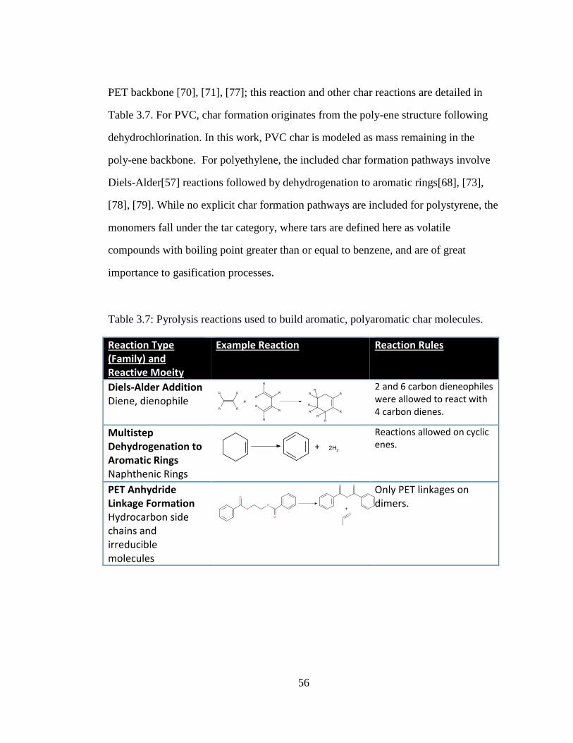
56

PET backbone [70], [71], [77]; this reaction and other char reactions are detailed in

Table 3.7. For PVC, char formation originates from the poly-ene structure following

dehydrochlorination. In this work, PVC char is modeled as mass remaining in the

poly-ene backbone. For polyethylene, the included char formation pathways involve

Diels-Alder[57] reactions followed by dehydrogenation to aromatic rings[68], [73],

[78], [79]. While no explicit char formation pathways are included for polystyrene, the

monomers fall under the tar category, where tars are defined here as volatile

compounds with boiling point greater than or equal to benzene, and are of great

importance to gasification processes.

Table 3.7: Pyrolysis reactions used to build aromatic, polyaromatic char molecules.

Reaction Type (Family) and Reactive Moeity

Example Reaction Reaction Rules

Diels-Alder Addition Diene, dienophile

2 and 6 carbon dieneophiles were allowed to react with 4 carbon dienes.

Multistep Dehydrogenation to Aromatic Rings Naphthenic Rings

2H2

Reactions allowed on cyclic enes.

PET Anhydride Linkage Formation Hydrocarbon side chains and irreducible molecules

Only PET linkages on dimers.

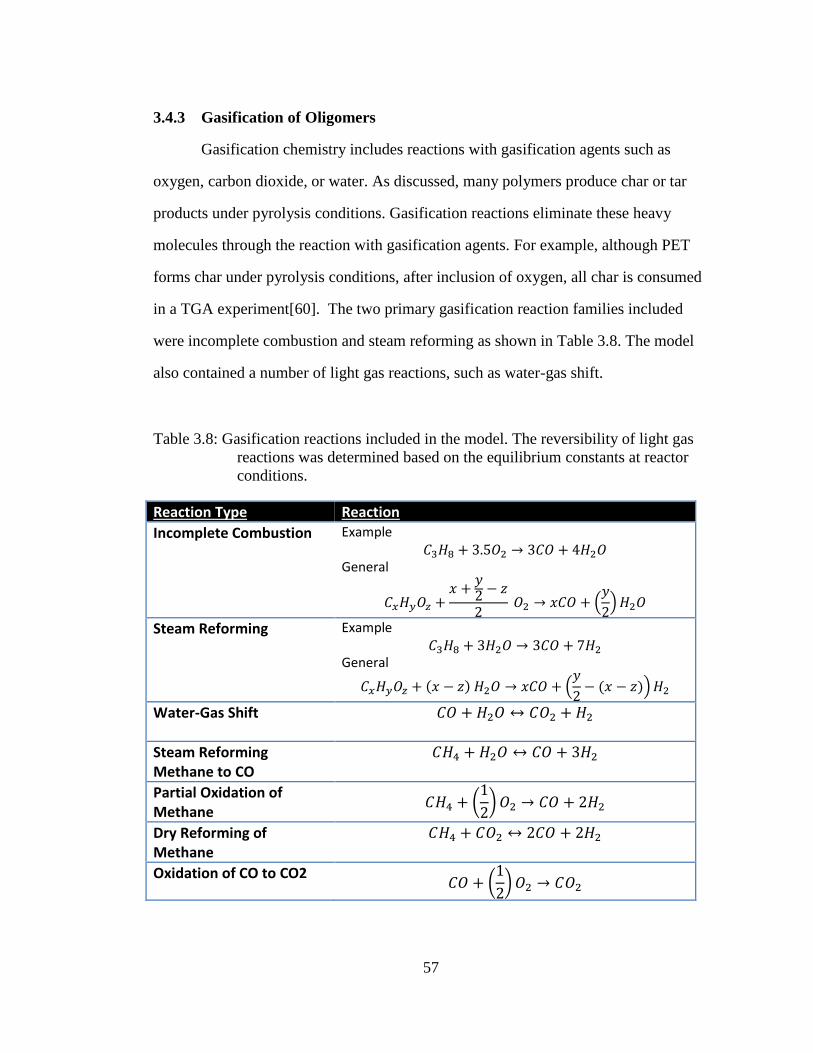
57

3.4.3 Gasification of Oligomers

Gasification chemistry includes reactions with gasification agents such as

oxygen, carbon dioxide, or water. As discussed, many polymers produce char or tar

products under pyrolysis conditions. Gasification reactions eliminate these heavy

molecules through the reaction with gasification agents. For example, although PET

forms char under pyrolysis conditions, after inclusion of oxygen, all char is consumed

in a TGA experiment[60]. The two primary gasification reaction families included

were incomplete combustion and steam reforming as shown in Table 3.8. The model

also contained a number of light gas reactions, such as water-gas shift.

Table 3.8: Gasification reactions included in the model. The reversibility of light gas

reactions was determined based on the equilibrium constants at reactor

conditions.

Reaction Type Reaction

Incomplete Combustion Example 𝐶3𝐻8 + 3.5𝑂2 → 3𝐶𝑂 + 4𝐻2𝑂

General

𝐶𝑥𝐻𝑦𝑂𝑧 +𝑥 +

𝑦2 − 𝑧

2 𝑂2 → 𝑥𝐶𝑂 + (

𝑦

2)𝐻2𝑂

Steam Reforming Example 𝐶3𝐻8 + 3𝐻2𝑂 → 3𝐶𝑂 + 7𝐻2

General

𝐶𝑥𝐻𝑦𝑂𝑧 + (𝑥 − 𝑧) 𝐻2𝑂 → 𝑥𝐶𝑂 + (𝑦

2− (𝑥 − 𝑧))𝐻2

Water-Gas Shift 𝐶𝑂 + 𝐻2𝑂 ↔ 𝐶𝑂2 + 𝐻2

Steam Reforming Methane to CO

𝐶𝐻4 + 𝐻2𝑂 ↔ 𝐶𝑂 + 3𝐻2

Partial Oxidation of Methane

𝐶𝐻4 + (1

2)𝑂2 → 𝐶𝑂 + 2𝐻2

Dry Reforming of Methane

𝐶𝐻4 + 𝐶𝑂2 ↔ 2𝐶𝑂 + 2𝐻2

Oxidation of CO to CO2 𝐶𝑂 + (

1

2)𝑂2 → 𝐶𝑂2

58

3.5 Network Generation

Using the depolymerization, pyrolysis, and gasification chemistries, the

reaction network was generated using in-house software tools. First, a reaction

network was made for the pyrolysis of each plastic oligomer using the Interactive

Network Generator, INGen[44], [80]. These networks were then merged together

using INGenNetworkMerge, a C# application; this application also added gasification

reactions to the network. Finally, link cleavage reactions (e.g., 𝑃𝐸𝐼𝐿 → 𝑃𝐸𝑆𝐶0 +

𝑃𝐸𝑆𝐶1) representing the breakdown of the polymer backbone were added manually to

the merged network. The features of the final reaction network are given Table 3.9.

In the final reaction network, the initial depolymerization contained reaction

families for each plastic, including four total families for the competition of

polystyrene depolymerization mechanisms. The pyrolytic breakdown of oligomers and

formation of tar and char molecules was described using five and three reaction

families, respectively. Finally, gasification included general incomplete combustion

and steam reforming reactions common to all plastics as well as a reaction family

specific to PET char breakdown. The final network containing 283 reactions and 85

species was used to build the kinetic model.

59

Table 3.9: Reaction network diagnostics for the plastics model.

Reaction Family Reaction Count

Adjustable Parameters

Constraints

Depolymerization PE Depolymerization 4 2 0 PET Depolymerization 4 2 0 PVC Depolymerization 3 2 0 Polystyrene Random Scission 102 2 0 Polystyrene Backbiting (dimer)

18 2 0

Polystyrene Backbiting (trimer)

17 2 0

Polystyrene Unzipping 19 2 0

Pyrolysis Acyclic Thermal Cracking 27 3 0 Decarboxylation 12 2 2 Decarbonylation 3 2 2 Ester Decarboxylation 2 2 2 Ester Rearrangement 2 2 0

Char Formation PET Anhydride Formation 6 2 0 Diels-Alder 4 2 0 Aromatic Ring Formation 4 2 0

Gasification Incomplete Combustion 19 2 0 Steam Reforming 18 2 2 PET Anhydride Breakdown 14 2 0 Light Gas Reactions 5 10 2

Total Reactions 283 Total Species 85

3.6 Model Equations and Kinetics

The reaction network was used to generate a set of material balance differential

equations with one equation per molecular species. This model was built and solved

using an in-house software, the Kinetic Model Editor (KME)[40]. In general, the rate

laws used standard mass-action kinetics and Arrhenius rate constants. Exceptions to

60

this rule were in the gasification reactions where the kinetics were assumed to be first

order with respect to oxygen and water for incomplete combustion and steam

reforming respectively.

The number of adjustable parameters in the model was reduced using the

concept of reaction families and linear free energy relationships (LFER). All reactions

in a given reaction family are modeled to have the same pre-exponential factor.

Furthermore, the activation energies are modeled to follow the Bell-Evans-

Polanyi[51], [52] LFER which relates activation energy of individual reactions to the

enthalpy of reaction. The final form of the rate constant, derived in prior work[42],

[48], is given in Equation 3.15 for reaction i and reaction family j. In general, this

constrains the number of adjustable parameters to three per reaction family; however

for this work, only acyclic thermal cracking utilizes 𝛼𝑗. All other reaction families

contained two adjustable parameters, Aj and E0(j). This modeling approximation states

that reaction rate constants for the reactions in the other families are equal for all

reactions in the family.

The number of adjustable parameters was further constrained using parameter

values from the open literature. In particular, constraints were placed on many of the

pyrolysis and gasification parameters. For pyrolysis, rate parameters from the

literature were utilized for decarboxylation and decarbonylation[74]. Ester

decarboxylation was modeled to have the same rate parameters as decarboxylation.

For gasification, reactions with oxygen are much faster than reactions with CO2 or

H2O. Steam reforming was constrained to be slower and proportional to incomplete

combustion. Finally, literature values were assumed for the water-gas shift[81].

ln 𝑘𝑖 = ln𝐴𝑗 − (𝐸0 (𝑗) + 𝛼𝑗 ∗ Δ𝐻𝑖

𝑅𝑇)

(3.15)

61

3.7 Model Evaluation

Literature studies provided the data to evaluate the kinetic model. The

polyethylene study was used to probe the kinetics of polyethylene degradation,

pyrolysis, gasification, and polyethylene char formation reactions. The PET study was

to demonstrate the ability of molecular-level models to predict thermogravimetric

analysis (TGA) experiments while analyzing the competition between polymer

breakdown, PET char formation, and PET char breakdown. The PVC study was used

to obtain rate constants for dehydrochlorination and the subsequent reaction producing

benzene. Finally, the polystyrene study allowed for the analysis of the competition

between the different depolymerization mechanisms.

3.7.1 Model Evaluation – PE

The polyethylene study utilized a pilot-plant scale fluidized bed gasifier using

both oxygen and steam as gasifying agents for polyethylene consumption[23]. The

experiments of interest are summarized in Table 3.10. Experimental runs 3-7 from this

study were selected because they were uncatalyzed and used air as the oxidation agent.

The reported results included input flow rates of polyethylene, air, output syngas

composition, and tar flow rate.

62

Table 3.10: Utilized experiments from Arena et al[23].

Run 3 Run 4 Run 5 Run 6 Run 7

Polyethylene Flow Rate (kg/hr)

16.7 21.8 27.9 20.0 31.0

Air Flow Rate (kg/hr) 64.3 77.2 90.1 90.1 90.1

Temperature (°C) 850 869 867 898 845

Syngas Composition (vol%)

N2 CO H2

CO2 CH4

C2Hx

68.7 2.7 7.4 9.5 8.3 3.4

65.7 2.5 9.1 9.6 8.8 4.4

64.6 2.4 9.6 9.6 9.1 4.6

69 2.3 8.3 10.4 7.1 2.9

63.9 2.8 9.1 9.1 10.4 4.8

Output Tar Flow Rate(kg/hr)

6.2 7.8 12.1 7.0 14.6

The model tuning results are shown in Figure 3.9. The C2Hx fraction was the

combined flow rate of ethane, ethylene, and acetylene. Tars were classified as

compounds with a boiling point greater than or equal that of benzene. The model

showed good agreement with experimental results with 𝑦𝑝𝑟𝑒𝑑𝑖𝑐𝑡𝑒𝑑 = 0.952 ∗

𝑦𝑒𝑥𝑝𝑒𝑟𝑖𝑚𝑒𝑛𝑡𝑎𝑙 + 0.0036. Figure 3.10 shows a comparison between experimental and

predicted liquid/gas mass ratio. The model results showed agreement with

experimental results, with small under-predictions on runs 5 and 7.

63

Figure 3.9: Tuning results for all data sets. The linear fit has the equation

ypredicted=0.952*yexperimental+0.0036. Tar yield is in units of (g/s/25); it was

rescaled to have a similar value as the light gas flow rates (mol/s).

Figure 3.10: Comparison of experimental and model predicted results for liquid/gas

ratio (mass basis) for all data sets.

In order to further examine deviations between model and experimental results,

the effects of uncertainty in the reported measurements were analyzed in Figure 3.11.

For GC measurements, the standard error was 0.05 vol% due to the number of

0.00E+00

2.00E-02

4.00E-02

6.00E-02

8.00E-02

1.00E-01

1.20E-01

1.40E-01

1.60E-01

1.80E-01

0 0.02 0.04 0.06 0.08 0.1 0.12 0.14 0.16 0.18

Methane

Hydrogen

Carbon Dioxide

Carbon Monoxide

C₂Hₓ

Tar Scaled

y=x

0.00

0.02

0.04

0.06

0.08

0.10

0.12

0.14

0.16

Run 3 Run 4 Run 5 Run 6 Run 7

Liq

uid

/Gas

Rat

io

Experimental

Predicted

64

reported significant figures in Arena et al[23]; similarly, the error in tar flow was 0.05

kg/hr. For tar, the model prediction is as good as the reported significant figures. The

experimental results reported an average temperature; however, minor temperature

deviations in the reactor are possible. To analyze these effects on model predictions, a

10 degree temperature variation was studied on Run 6. The results were shown to be

relatively insensitive to minor changes in temperature, implying that deviations from

the average temperatures in Table 3.10 would have little impact on modeling results.

Figure 3.11: Experimental error and the effects of temperature deviation in model

predictions for Run 6. Effects of a 10 degree temperature variation are

shown using error bars.

3.7.2 Model Evaluation – PET

For polyethylene terephthalate, a thermogravimetric analysis (TGA) [60] study

with oxidative depolymerization provided TGA curves for different heating rates of

0

0.02

0.04

0.06

0.08

0.1

0.12

Methane Hydrogen Carbon Dioxide CarbonMonoxide

C₂Hₓ Tar Scaled

Experimental Predicted

65

PET using air as the carrier gas. This allowed for the analysis of PET

depolymerization, char formation, and subsequent char breakdown with oxygen. A

software tool was developed in order to utilize TGA data in a molecular-level kinetic

model.

The simulation of TGA with a molecular-level kinetic model was performed

using an in-house software called TGA Simulator; a C# application developed for this

work. The logic for the TGA simulator is given in Figure 3.12. In order to simulate a

constant heating rate, TGA Simulator repeatedly calls the ODE solver (within KME)

using isothermal runs for short duration where the output of one simulation is the input

to the next simulation. For example, if the heating rate is 10K per minute starting at

298K then TGA simulator would integrate for 6 seconds at 298K, 6 seconds at 299K,

and so forth. The TGA Simulator predicts mass-loss based on the molar amounts,

boiling points, and flow rates of each component.

Figure 3.12: Logic for the TGA Simulator C# application

The results in Figure 3.13 show the experimental and predicted TGA curves.

There are three regions of interest on this graph: the initial mass loss, char formation,

and char consumption. The majority of the initial drop is due to PET

66

depolymerization; however, any reaction that causes molecular breakdown also plays

a role in the initial region of the curve. The relative rates between the breakdown

chemistry and PET anhydride formation determine the amount of char initially

formed. The char consumption is known to occur under gasification conditions. For

instance, an analogous study by Du and coworkers on pyrolysis showed a persistent

char.[76] Similarly, Figure 3.14 shows remaining char when oxygen is removed from

the simulation. Because our results are the combination of many reaction families and

rate parameters, it is difficult to draw a connection to parameters derived from

traditional TGA analyses; however, the fit of the raw data implies agreement between

experiment and model results.

Figure 3.13: TGA model results (lines) compared with experiment (points). Colors

correspond to different heating rates: red, 5 °C/min; green, 10 °C/min;

blue, 20 °C/min; orange, 40 °C/min. The left plot gives the TGA curves,

the right plot is a parity plot of the results. The maximum decomposition

rates in units of wt%/°C are 0.018, 0.17, 0.015, and 0.041 in order of

increasing heating rate.

67

Figure 3.14: TGA Simulator results showing persistence of char in the absence of

oxygen for PET depolymerization at a heating rate of 40 °C/min.

3.7.3 Model Evaluation – PVC

The tuning effort for PVC was focused on a study in a bubbling fluidized bed

to probe the kinetics of dehydrochlorination and PVC char formation[82]. In this

study, there were two uncatalyzed experiments and five catalyzed experiments. In

general, the experiments of interest are uncatalyzed as this is more similar to

applications such as MSW gasification. However, dehydrochlorination is known to be

fast[68], [73] and kinetics are not expected to be limiting which allows for the usage

of all seven experiments. The catalyst does affect char formation and therefore only

uncatalyzed data sets were used for char analysis.

68

Table 3.11: HCl and char from all experiments in Slapak et al.[82] Q1 and Q2 are

uncatalyzed (quartz sand bed). A1, A2, and all A3 experiments were

under alumina support. *- data points not used in char analysis due to

catalyst effects on char formation.

Experiment HCl (wt% PVC) Char (wt% PVC)

Q1 54 35

Q2 35.2 33

A1 57 16*

A2 54 16*

A3-1150K A3-1200K A3-1250K

54 54 54

16* 9* 3*

Results from PVC kinetic parameter tuning are given in Figure 3.15. The char

predictions for the two uncatalyzed experiments matched well with the experimental

data. For HCl, six of the seven data sets were predicted well. The remaining data

point, Q2, is expected to be an outlier or a typographical error because it is well

known that approximately 55 wt% of PVC is quickly released in the initial

depolymerization step[68], [73].

69

Figure 3.15: Results for HCl (all runs) and Char (only Q1 and Q2). The outlet flow

rate units for HCl and char are in mol/s and g/s/50 respectively.

3.7.4 Model Evaluation – PS

The polystyrene tuning study focused on the probing the different

depolymerization mechanisms using literature on pyrolysis in a fluidized bed[67]. The

results of interest were relative amounts of mono-, di-, and triaromatics after

pyrolysis over a range of temperatures, as shown in Table 3.12. The kinetic parameters

were tuned to these data sets with results shown in Figure 3.16. Overall the fit was

good with 𝑦𝑝𝑟𝑒𝑑𝑖𝑐𝑡𝑒𝑑 = 0.9595𝑦𝑒𝑥𝑝𝑒𝑟𝑖𝑚𝑒𝑛𝑡𝑎𝑙 + 0.0217. The largest deviation was

seen in the 450 °C data set. This data set is less important as the temperature in most

gasification applications is significantly higher.

0.00E+00

2.00E-05

4.00E-05

6.00E-05

8.00E-05

1.00E-04

Ou

tlet

Flo

w R

ate

Predicted Experimental

70

Table 3.12: Experimental weight percent values for monoaromatics, diaromatics and

triaromatics in pyrolysis output at different temperatures[67]. All values

are in weight percent of initial polystyrene.

Temperature Monomer Dimer Trimer

450 °C 72 11 14

500 °C 76 13.5 7

550 °C 79 15 2

600 °C 87 12 ---

Figure 3.16: Parity plot for monomer-trimer predictions for polystyrene pyrolysis. A

least-squares linear fit of the data gives ypredicted = 0.9595yexperimental +

0.0217

3.7.5 Reaction Family Rate Constants

After evaluation and optimization with all data sets, a tuned set of kinetic

parameters was developed and are given in Table 3.13. In this table, the rate constants

are relative to the rate constant for Acyclic Thermal Cracking.

0

0.2

0.4

0.6

0.8

1

1.2

0 0.1 0.2 0.3 0.4 0.5 0.6 0.7 0.8 0.9 1

Pre

dic

ted

Wei

ght

Per

cen

t

Experimental Weight Percent

450°C500°C550°C600°C

71

Table 3.13: Reaction family rate constants at 1000 K relative to Acylic Thermal

Cracking. log(k)relative,1000=log(k)AcylicThermalCracking,1000-

log(k)ReactionFamily,1000.

Reaction Family 𝐥𝐨𝐠(𝐤)𝐫𝐞𝐥,𝟏𝟎𝟎𝟎

Depolymerization PE Depolymerization 1.60 PET Depolymerization -2.57 PVC Depolymerization - Dehydrochlorination

-1.95

PVC Depolymerization - Benzene Formation

-8.17

Polystyrene Random Scission -2.95 Polystyrene Backbiting (dimer) -7.63 Polystyrene Backbiting (trimer) -2.49 Polystyrene Unzipping -5.34 Pyrolysis Acyclic Thermal Cracking 0.00 Decarboxylation 2.40 Decarbonylation 2.40 Ester Decarboxylation 2.40 Ester Rearrangement -2.58 Char Formation

PET Anhydride Formation 1.98 Diels-Alder -2.83 Aromatic Ring Formation -0.76 Gasification Incomplete Combustion -4.00 Steam Reforming -7.30

PET Anhydride Breakdown -1.92 Light Gas Reactions Water-gas Shift -6.83 Oxidation CO to CO2 -3.14 Partial Oxidation of Methane (forward) -7.10

Steam Reforming of Methane (reversible) -5.90 Dry Reforming of Methane (reversible) -6.84

72

3.8 Conclusions

A molecular-level kinetic model was developed for the gasification of four

common plastics: PE, PVC, PET, and PS. The model’s parameters were tuned using

literature studies on each of the plastics. The model includes the kinetics of the

formation and degradation of tar and char molecules from these wastes, which are

important design considerations for waste-to-energy technologies such as MSW

gasification.

Furthermore, because this model is at the molecular-level, it can be used to

help predict changes in syngas composition in the gasifier outlet as a function of the

MSW composition. This could be used to help process engineers design better waste

streams for a gasification unit. The robustness of a molecular-level model is especially

important in the application of MSW because the waste composition is likely to

change as a function of season and location. Only models containing fundamental

chemistry have a hope of modeling such a diverse set of conditions.

73

MOLECULAR-LEVEL KINETIC MODELING OF BIOMASS

GASIFICATION

Scott R. Horton1, Rebecca Mohr2, Yu Zhang2, Francis Petrocelli2, and Michael T. Klein1

1University of Delaware Energy Institute and Department of Chemical and


Reproduced by permission from Horton, S.R.; Mohr, R.; Zhang, Y.; Petrocelli, F.;

Klein, M.T. “Molecular-level kinetic modeling biomass gasification.” Energy &

Fuels. 2015 (Web). 10.1021/acs.energyfuels.5b01988. Copyright 2015. American

Chemical Society.[83]

Chapter 4

74

4.1 Abstract

A molecular-level kinetic model for biomass gasification was developed and

tuned to experimental data from the open literature. The development was divided into

two categories: the composition of the feedstock and the construction of the reaction

network. The composition model of biomass was divided into three submodels for

cellulose, hemicellulose, and lignin. Cellulose and hemicellulose compositions were

modeled as linear polymers using Flory-Stockmayer statistics to represent the polymer

size distribution. The composition of lignin, a cross-linked polymer, was modeled

using relative amounts of structural building blocks, or attributes. When constructing

the full biomass composition model, the fractions of cellulose, hemicellulose, and

lignin were optimized using literature-reported ultimate analyses.

The reaction network model for biomass contained pyrolysis, gasification, and

light-gas reactions. For cellulose and hemicellulose, the initial depolymerization was

described using Flory-Stockmayer statistics. The derived monomers from cellulose

and hemicellulose were subjected to a full pyrolysis and gasification network. The

pyrolysis reactions included both reactions to decrease molecule size, such as thermal

cracking, and char formation reactions, such as Diels-Alder addition. Gasification

reactions included incomplete combustion and steam reforming. For lignin, reactions

occurred between attributes and included both pyrolysis and gasification reactions.

The light-gas reactions included water-gas shift, partial oxidation of methane,

oxidation of carbon monoxide, steam reforming of methane, and dry reforming of

methane. The final reaction network included 1356 reactions and 357 species.

The performance of the kinetic model was examined using literature data that

spanned six different biomass samples and had gas compositions as primary results.

Three data sets from different biomass samples were used for parameter tuning, and

75

parity plot results showed good agreement between the model and data (𝑦𝑝𝑟𝑒𝑑𝑖𝑐𝑡𝑒𝑑 =

𝑦𝑜𝑏𝑠 ∗ 0.928 + 0.0003). The predictive ability of the model was probed using three

additional data sets. Again, the parity plot showed agreement between model and

experimental results (𝑦𝑝𝑟𝑒𝑑𝑖𝑐𝑡𝑒𝑑 = 𝑦𝑜𝑏𝑠 ∗ 0.989 − 0.007).

4.2 Introduction

Biomass is the major source of chemical energy that is renewable at a

reasonable timescale. The most common way to access that energy is incineration;

however, there are technical and environmental issues with large scale

implementation. In terms of technical feasibility, biomass has much lower energy

density than its fossil fuel counterparts[84]. Environmentally, the incineration of

biomass has high production of harmful oxygenates such as dioxins and furans[85].

The gasification of biomass has gained interest in recent years due to lower emissions

of pollutants and the production of synthesis gas (syngas), a possible route to liquid

fuels. Biomass gasification also makes up the majority of municipal solid waste

(MSW) gasification, an up-and-coming waste disposal technology. In the design of

biomass gasification units, important parameters are tar production and syngas

composition. To study these parameters, kinetic models are often utilized in the

literature.

Previous kinetic models of biomass gasification are lumped in nature[86],[87].

Lumped models contain no structural information beyond the definition of the lump.

For instance, a lumped model might contain ‘Tar’ where tar is simply defined as

‘liquid product at reactor conditions’. Lumped models in the literature follow some

combination of parallel or sequential implementations, as shown in Figure 4.1. More

advanced lumped models contain light gasses explicitly. For example, Zhong et al.[88]

76

contained reactions and material balances for many of the observed light gasses.

However, the model is still fundamentally lumped as there is no chemical description

from the feedstock molecules (e.g., cellulose) to light gas. More examples of kinetic

models found in literature can be found in a reviews by Puig-Arnavat[16] and

Prakash[89].

Figure 4.1: Literature lumped kinetic models. (Left) Sequential lumped model[86] of

biomass gasification. (Right) parallel lumped model of biomass

gasification where V1-V5 are lumped volatile products.[87]

Chemical percolation devolatilization (CPD) was developed by Fletcher and

coworkers in the early 1990s and has been utilized for two decades in work on the

pyrolysis and gasification of coal[90]–[92]. Due to the molecular similarity between

coal and lignin, CPD has been successfully applied to biomass in recent years[93]–

[95]. In CPD, the chemical structure of the feedstock is modeled as aromatic clusters,

labile bridges, and side chains, and the cluster size distribution is described Bethe

lattice statistics. The kinetic breakdown of the lattice involves the cleavage of labile

bridges into side chains, and the production of light gas, char, and tar molecules. A

key advantage of CPD is the direct usage of measurable structural parameters and

simple, easy-to-understand kinetic networks. Also, the usage of lattice statistics is

77

appropriate for cross-linked polymers such as lignin. The main drawbacks of CPD are

the minimal information on the molecular descriptions of tar and light gas, and the

application of lattice statistics onto predominantly linear polymers such as cellulose

and hemicellulose.

For similar reactor conditions on a single biomass sample, lumped kinetic

models do an adequate job of describing experimental data[15], [96]. Problems arise

when the feedstock or reactor conditions are perturbed. For example, a lumped model

of pine sawdust will have different parameters than a lumped model of grass.

Fundamentally, a model can only answer questions at the same level of complexity as

the model’s definition. For example, a lumped model with a single ‘tar’ component

cannot yield any information about the specific tars present in the output stream. In

MSW gasification, the biomass feedstock changes over the course of time. For these

changes, the questions that are asked of the model are at the molecular-level, and

therefore the model must retain the same level of detail.

The current modeling work is the first representation of a molecular-level

kinetic model of biomass gasification. This model maps the feedstock to products,

tracking each individual molecular species throughout the reactor. With this in mind,

there are three fundamental steps to building a molecular-level kinetic model for

biomass gasification. First, the feedstock must be defined as a set of molecules.

Second, a reaction network describes how the feedstock becomes products. Third, a

kinetic model is built which utilizes the feedstock and reaction network to create a

system of mass balance differential equations. The output of this process is a model

with a set of rate parameters for each reaction chemistry. These rate parameters are

then tuned, or optimized, using experimental data from the open literature.

78

The most interesting results from the model are also at the molecular-level. For

example, the model contains reaction chemistries important to biomass gasification.

These chemistries convey an underlying understanding of the reactor. Second, the

model contains explicit molecular definitions of tar molecules. The amount of

produced tar can then be predicted for a range of conditions. Third, the model can

predict relative changes in syngas and tar compositions for a variety of biomass

feedstocks. This allows for the anticipation of changes in syngas output due to changes

in the MSW feedstock composition.

4.3 Molecular Representation of Biomass

In order to model reactor kinetics at the molecular-level, the feedstock must

first be represented as a set of molecules and mole fractions. For biomass, an explicit

composition cannot be measured experimentally because it contains large polymeric

structures; therefore, composition models are required to map available experimental

data to molecular compositions.

A molecular-level composition model fundamentally obtains a list of

molecules and mole fractions. Here, a composition model is a set of probability

distribution functions (PDFs) that describe the relative amounts molecular groups,

called attributes within the feed stream. For linear polymers (e.g., cellulose), where

the monomer structure is relatively well understood, the composition was modeled

with the traditional Flory distribution function[61]. For cross-linked polymers with

variable repeat units such as lignin, a more elaborate set of PDFs must be constructed.

For both simple and complex systems, the optimal set of PDFs is determined by

tuning the PDF parameters to experimental measurements through structure-property

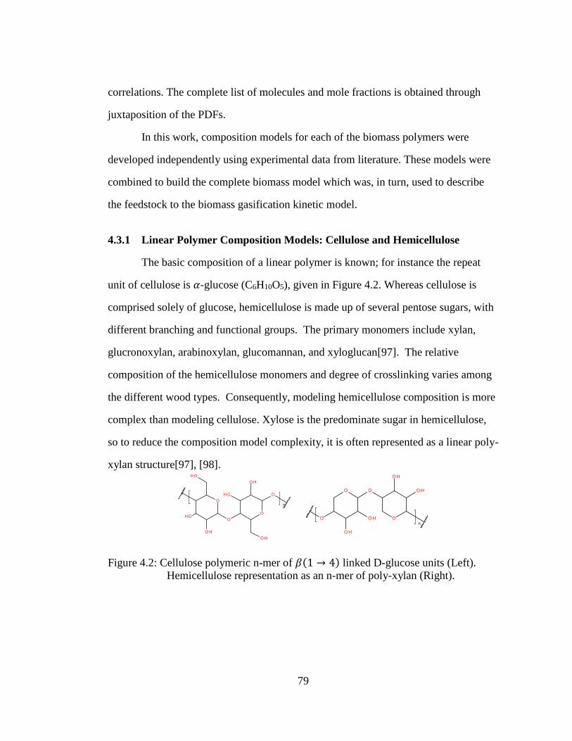
79

correlations. The complete list of molecules and mole fractions is obtained through

juxtaposition of the PDFs.

In this work, composition models for each of the biomass polymers were

developed independently using experimental data from literature. These models were

combined to build the complete biomass model which was, in turn, used to describe

the feedstock to the biomass gasification kinetic model.

4.3.1 Linear Polymer Composition Models: Cellulose and Hemicellulose

The basic composition of a linear polymer is known; for instance the repeat

unit of cellulose is 𝛼-glucose (C6H10O5), given in Figure 4.2. Whereas cellulose is

comprised solely of glucose, hemicellulose is made up of several pentose sugars, with

different branching and functional groups. The primary monomers include xylan,

glucronoxylan, arabinoxylan, glucomannan, and xyloglucan[97]. The relative

composition of the hemicellulose monomers and degree of crosslinking varies among

the different wood types. Consequently, modeling hemicellulose composition is more

complex than modeling cellulose. Xylose is the predominate sugar in hemicellulose,

so to reduce the composition model complexity, it is often represented as a linear poly-

xylan structure[97], [98].

Figure 4.2: Cellulose polymeric n-mer of 𝛽(1 → 4) linked D-glucose units (Left).

Hemicellulose representation as an n-mer of poly-xylan (Right).

80

Composition models are required for linear polymers due to polydispersity,

i.e., the presence of differently sized n-mers, and their molecular composition is

described using a polymer-size distribution function. In this model, a Flory

distribution[61] is used due to its simplicity and wide-spread usage.

𝑥𝑛 = (1 − 𝑝) ∗ 𝑝𝑛−1 (4.1)

The Flory distribution is given in Equation 4.1, where p is the bridge fraction,

or fraction of end-groups that are linkages. Linear polymers can be thought of as

cores, side chains (SCs) and inter-core linkages (ILs), a verbiage that will be used later

in the analysis of the statistics in cross-linked polymers. By considering each repeat

unit as a core, it follows that SCs and ILs are terminal substituents and bridges

between cores, respectively. A monomer, therefore, is a core with two SCs, and a

dimer contains 2 cores, two SCs, and 1 IL. When this concept is extended to a general

linear polymer, an 𝑛-mer has (𝑛 − 1) ILs, two SCs, and 𝑛 cores. The concentration of

sites in the system is given by Equation 4.2 since every IL represents two previously

reactive sites and all unreacted sites are [SC]. The bridge fraction in terms of SCs and

ILs is given by Equation 4.3.

𝑆𝑖𝑡𝑒𝑠 𝑖𝑛 𝑡ℎ𝑒 𝑆𝑦𝑠𝑡𝑒𝑚 = 2 ∗ [𝐼𝐿] + [𝑆𝐶] (4.2)

𝑝 =2 ∗ [𝐼𝐿]

2 ∗ [𝐼𝐿] + [𝑆𝐶]

(4.3)

In order to model the molecular composition of a linear polymer using a Flory

distribution, the value for p is estimated from experimental measurements. Literature

studies have used a variety of methods to characterize a linear polymer. One common

metric is the average degree of polymerization, or 𝑋𝑛̅̅̅̅ , which can be related to 𝑝 using

Equation 4.4. In biomass gasification literature, the most common representation of

81

feedstock compositional information is an ultimate analysis. For example, an ultimate

analysis for a cellulose sample is shown in Table 4.1.

𝑋𝑛̅̅̅̅ =1

1 − 𝑝

(4.4)

Table 4.1: Ultimate analysis of cellulose samples in Chang et al. (2011)[99].

Element Chang et al. (2011)

C (wt%) 44.44 H (wt%) 6.17 O (wt%) 49.38

Given a value for p (or equivalently 𝑋𝑛̅̅̅̅ ), a predicted ultimate analysis can be

calculated through the use of Flory statistics. First, the mole fraction of each n-mer is

calculated using Equation 4.1. Second, the weight fraction of each n-mer is calculated

by using the average molecular weight of the polymer, 𝑀𝑊̅̅ ̅̅ ̅̅ , as shown in using

Equation 4.5. Finally, the ultimate analysis is calculated by multiplying the mass

fraction of each n-mer by the mass fraction of each element in the n-mer. For

example, the predicted weight percent of carbon is found using Equation 4.6. Using

this method, an ultimate analysis can be predicted for a given 𝑋𝑛̅̅̅̅ and polymer.

𝑤𝑛 = 𝑥𝑛 ∗𝑀𝑊𝑛

𝑀𝑊̅̅ ̅̅ ̅̅

(4.5)

𝑝𝑟𝑒𝑑𝑖𝑐𝑡𝑒𝑑 𝑤𝑡% 𝐶𝑎𝑟𝑏𝑜𝑛 = ∑𝑤𝑛 ∗ 𝐶𝑤𝑡%,𝑛−𝑚𝑒𝑟

∞

𝑛=1

𝑤ℎ𝑒𝑟𝑒 𝐶𝑤𝑡%,𝑛−𝑚𝑒𝑟 𝑖𝑠 𝑡ℎ𝑒 𝑤𝑒𝑖𝑔ℎ𝑡 𝑝𝑒𝑟𝑐𝑒𝑛𝑡 𝑜𝑓 𝑐𝑎𝑟𝑏𝑜𝑛 𝑖𝑛 𝑡ℎ𝑒 𝑛 − 𝑚𝑒𝑟

(4.6)

An automated tool called Linear Polymer Composition Editor has been

developed in a C# application to facilitate the optimization of 𝑋𝑛̅̅̅̅ for any linear

82

polymer and experimental data set. This tool works using a simple optimization loop

as shown in Figure 4.3. First, it guesses a value for the degree of polymerization. Next

it calculates an ultimate analysis for this degree of polymerization. It then compares to

experimental results using a least-squares objective function. Finally, it adjusts the

prediction.

Figure 4.3: Linear Polymer Composition Editor optimization loop.

The linear polymer composition editor was used to simulate the compositions

of cellulose and hemicellulose. The composition simulated by the Flory distribution

fits very well with the literature as shown in Table 4.2. The agreement is expected as

cellulose is known to be composed of a single monomer unit and linear. With

hemicellulose, the Flory distribution still fits well; deviations between prediction and

experiment are likely due to cross-linking and the exclusion of other possible

monomeric units. However, if a mass balance can be achieved using the simpler

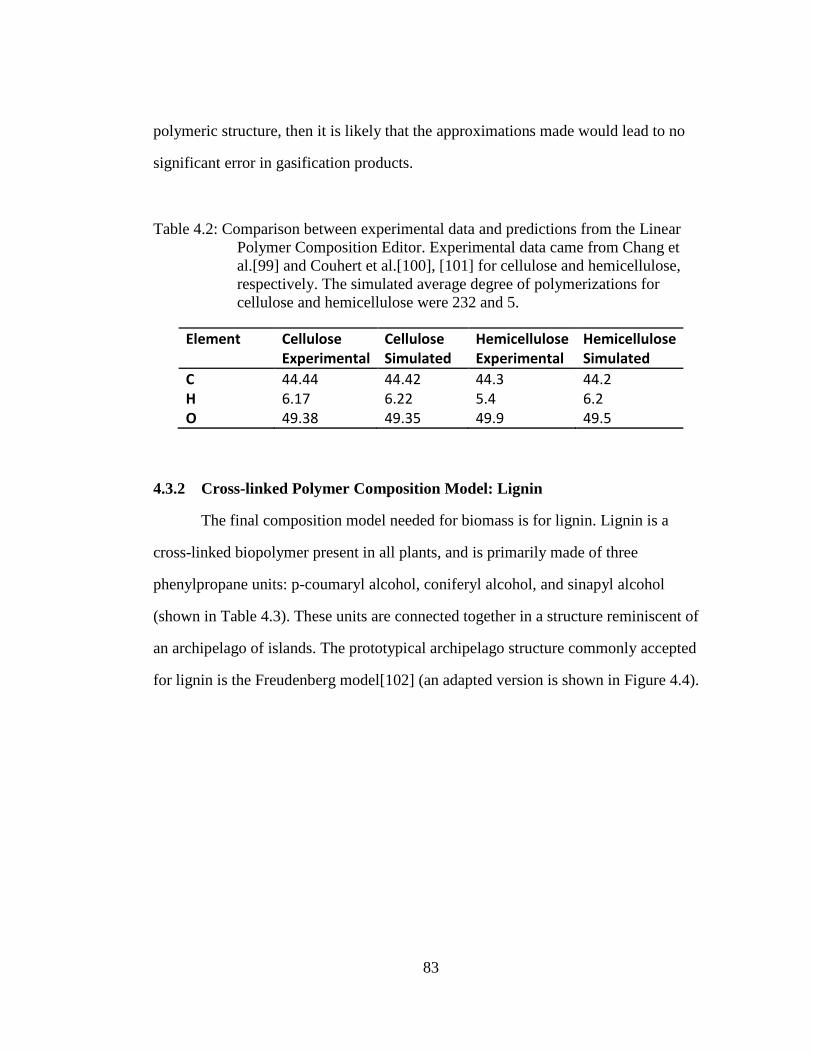
83

polymeric structure, then it is likely that the approximations made would lead to no

significant error in gasification products.

Table 4.2: Comparison between experimental data and predictions from the Linear

Polymer Composition Editor. Experimental data came from Chang et

al.[99] and Couhert et al.[100], [101] for cellulose and hemicellulose,

respectively. The simulated average degree of polymerizations for

cellulose and hemicellulose were 232 and 5.

Element Cellulose Experimental

Cellulose Simulated

Hemicellulose Experimental

Hemicellulose Simulated

C 44.44 44.42 44.3 44.2 H 6.17 6.22 5.4 6.2 O 49.38 49.35 49.9 49.5

4.3.2 Cross-linked Polymer Composition Model: Lignin

The final composition model needed for biomass is for lignin. Lignin is a

cross-linked biopolymer present in all plants, and is primarily made of three

phenylpropane units: p-coumaryl alcohol, coniferyl alcohol, and sinapyl alcohol

(shown in Table 4.3). These units are connected together in a structure reminiscent of

an archipelago of islands. The prototypical archipelago structure commonly accepted

for lignin is the Freudenberg model[102] (an adapted version is shown in Figure 4.4).

84

Table 4.3: C9 units of Lignin[103].

Name Coniferyl Alcohol Sinapyl Alcohol P-coumaryl Alcohol

Structure

85

Figure 4.4: Adapted Freudenberg Structure[102]. This structure was parsed to yield

the attribute identities.

The Freudenberg model was parsed to obtain identities of cores, ILs, and SCs.

The above structure contains 5 cores, 5 ILs, and 5 SCs, shown in Table 4.4. For the

O

O OH

O HO

O

OHO

OH

O

OH

OHO

HO

O

O

OH

OH

O

HO

O

OH

O

O

O

OOH

O

O

O

O

OH

O

O

O

OH

HOO

OH

OH

O

O

O

O

OH

OH

O

O

HO

OH

O

O

OH

OOH

OH

O

O

O

86

core attributes, there are two characteristics of note. First, the Ph-O bond for a

hydroxyl group on an aromatic is a strong bond; therefore, the OH groups are

considered part of a core. Similarly, C-C bonds where both carbons are part of

separate ring structures, e.g. biphenyl linkages, were considered strong bonds. When

parsing inter-core linkages, any IL bonded to three rings in the Freudenberg structure

was approximated to contain only two binding sites. This simplifies the configuration

of larger core clusters.

87

Table 4.4: Attribute Identities as parsed by CME from the Freudenberg model for

lignin.

Index Core Identity

IL Identity SC Identity

1

2

3

4

5

Lignin adds complexity to the binding site concept because not all side chains

and linkages can bind to all binding sites. An example is seen with side chain binding

to the phenol core, given in Figure 4.5. Based on the structure of the C9 units in Table

4.3, the two binding sites ortho to the hydroxyl group can only contain methoxy side

chains. The para binding site, on the other hand, must contain a C-C bond, or one of

88

the other four side chains. Each attribute was associated with R1 and R2 binding sites

based on the chemical structure.

Figure 4.5: Binding site types on the phenol core.

The molecular nature of the composition is retained despite the use of

attributes. Individual molecule identities and mole fractions are obtained through the

sampling five PDFs. The first three are attribute group PDFs, or the relative amounts

of each entry in Table 4.4. Each core has binding sites which can be filled by an IL,

SC, or left unfilled (-H side chain). This complexity gives rise to two additional PDFs.

First, a polymer size distribution defines the relative amounts of differently sized n-

core clusters; or a molecule with n cores and n-1 ILs. Finally, the binding site

distribution describes how many sites on each core cluster are filled by side chains.

The mole fractions of individual molecules are calculated through the combined

probabilities from each PDF as shown in Table 4.5. The complete juxtaposition of all

five PDFs gives both identities and mole fractions for the molecule list.

89

Table 4.5: Mole fraction calculation from sampled molecules.

Molecule Attributes Filled

Binding

Sites

Cluster

Size

Mole Fraction

Cores SCs and ILs

2 1 ∝

Pcore( )PSC(

)2 *

PBS(2)PCluster(1)

1 2 ∝ Pcore( )

Pcore( ) *

PIL( )

PSC( )2 *

PBS(1)PCluster(2)

In order to model the composition of lignin, experimental measurements were

obtained from literature. Compositional measurements of lignin have a strong

dependence on the lignin isolation method. For example, Kraft lignin comes from the

Kraft pulping process and is significantly degraded from the original plant matter. A

less destructive isolation technique is called Milled Wood Lignin (MWL) and the

product is considered to be the closest to native lignin[104]. Table 4.6 shows a subset

of the experimental measurements on miscanthus, a perennial grass[104].

90

Table 4.6: Experimental Data used in the optimization of the lignin compositional

model. All data are from Hage et al. (2009)[104].

Description Value Experiment

Ultimate Analysis (wt%) C H O N S

63.5 5.7 29.2 0.2 0.0

Unreported

Normal Molecular Weight (g/mol)

8300 Gel Permeation Chromatography

Aromatic H per ring 2.5 Carbon NMR

Methoxy (-OCH3) per ring 0.98 Carbon NMR

Phenolic OH per ring 0.28 Proton NMR

The optimization of lignin’s composition was performed using an in-house

software, the Composition Model Editor (CME)[43]. Each attribute PDF was modeled

using a histogram. Gamma distributions were used to determine the number of filled

binding sites on molecules and the polymer size distribution.

For any well-posed optimization problem, the number of adjustable parameters

should not exceed the number of data points and constraints. For this simulation, there

are 16 total adjustable parameters, and 6 usable data points shown in Table 4.7.

Therefore, to have a well-posed problem, 10 constraints must be applied. First,

average molecular weight (MW) is primarily controlled by the polymer size

distribution. Therefore, the standard deviation was set to a representative value and the

MW mean was allowed to vary. Similarly, the only data relevant to the binding site

distribution, which controls the number of side chains, is the number of aromatic

hydrogen per ring Again, a representative value was used for the standard deviation

and the number of aromatic hydrogens per ring was allowed to vary.

91

Constraints on the histogram were made using the relative amounts of

attributes group members within the Freudenberg structure, as shown in Table 4.7.

Two simulations were run to compare a fully constrained model to a second that

includes two additional degrees of freedom. In simulation 1, all attribute histograms

were set using the Freudenberg structure and only the polymer size distribution mean

and the binding site distribution mean were allowed to vary. The results, shown in

Table 4.8, were surprisingly accurate given that the attribute PDFs were set entirely

using the Freudenberg structure.

In the second simulation, the attribute PDFs were informed by the Freudenberg

structure, but selected attribute group member concentrations were allowed to vary.

For example, in the SC PDF, the composition of SC1 was allowed to vary and the

remaining side chains amounts were constrained to follow the Freudenberg structure

(e.g., the probabilities of SC2 and SC3 were equal). Of the substituent PDFs, the

methoxy side chain and phenol core were allowed to vary. These decisions were made

based on the experimental measurements available. The methoxy side chain correlates

very well with the experimentally measured ‘methoxy per ring’ datum, and the phenol

core is well described using the ‘phenolic OH per ring’ datum.

92

Table 4.7: Adjustable parameters in optimization. *obtained by difference, not an

adjustable parameter. In simulations 1 and 2, bolded terms were

optimized on.

Adjustable Parameter Simulation 1: Attribute PDFs from Freudenberg

Simulation 2: Attribute PDFs

partially constrained by Freudenberg

Polymer Size Distribution (Gamma)

Mean Standard deviation

32 5

34 5

Binding Site Distribution (Gamma)

Mean Standard Deviation

66 20

66 20

Core Histogram C1 C2 C3 C4

C5*

0.571 0.214 0.071 0.071 0.071

0.64 0.18 0.06 0.06 0.06

IL Histogram IL1 IL2 IL3 IL4

IL5*

0.2 0.1 0.1 0.5 0.1

0.2 0.1 0.1 0.5 0.1

SC Histogram SC1 SC2 SC3 SC4

SC5*

0.783

0.0435 0.0435 0.870

0.0435

0.89

0.022 0.022 0.044 0.022

Constraint Analysis 16 Adjustable parameters, 6 data points, 14

constraints.

16 Adjustable parameters, 6 data

points, 12 constraints.

93

The results from the second simulation are an improvement on the first

simulation especially on the methoxy correlation as shown in Table 4.8. This is

unsurprising as lignin from different sources primarily differ in the ratios of guaiacyl,

syringil, and p-coumryl units[97]. These units are differentiated based on the number

of methoxy groups. Therefore, it is follows that the probability of a methoxy side

chain would play a key role in tuning to a new biomass type.

Table 4.8: Experimental data currently used in the optimization of the lignin

compositional model. All data are from Hage et al. (2009)[104]. The data

shown here is a subset of data reported; CME adjustments are required to

make use of more data.

Description Experimental Value

Simulation 1: Attribute PDFs

from Freudenberg

Simulation 2: Attribute PDFs partially

constrained by Freudenberg

Ultimate Analysis (wt%) C H O N S

63.5 5.7

29.2 0.2 0.0

64.98 6.14

28.85 0.0 0.0

64.77 6.18

29.05 0.0 0.0

Average Molecular Weight (g/mol)

8300 8225.7 8304

Aromatic H per ring 2.5 2.44 2.47 Methoxy (-OCH3) per ring

0.98 0.897 0.98

Phenolic OH per ring 0.28 0.315 0.28

94

4.3.3 Combined Biomass Composition Model

A full biomass sample contains fractions of cellulose, hemicellulose, and

lignin. However, literature studies rarely report these fractions, and instead report an

ultimate analysis on the full biomass sample. In order to make use of these data, the

percentages of each subcomponent, reproduced in Table 4.9, are optimized such that

the net ultimate analysis agrees with experimental data.

Table 4.9: Ultimate analysis for each subcomponent of biomass from preceding

sections.

Element Cellulose Hemicellulose Lignin

C 44.4 44.3 64.77 H 6.2 6.2 6.18 O 49.4 49.5 29.05

In order to automate this process, an in-house C# application called MSW Bulk

Composition Solver was developed and utilized. The general logic and equations for

the calculation of the ultimate analysis of biomass are given in Figure 4.6. This

application, developed for optimizing municipal solid waste (MSW) cuts based on a

bulk ultimate analysis, can also be applied to biomass by simply setting all other

fractions of MSW to zero. This tool was used to find the optimal fractions, shown in

Table 4.10, of cellulose, hemicellulose, and lignin for six biomass samples from Li et

al., the gasification study used for the reaction kinetic model. The results showed good

agreement with experimental data for C, H, and O. The experimental results showed

trace amounts of nitrogen and sulfur that were not included in the model. We have

excluded N and S containing function groups due to their relatively insignificant

amounts and absence of both composition and gasification experimental results. The

95

future availability of more detailed experimental data could allow for the inclusion of

these functional groups.

Figure 4.6: Logic of MSW Bulk Composition solver applied for biomass. All numbers

in this figure are in wt%. The plastics and carbon support segments of the

figure are truncated as the weight fraction within biomass is 0 for each. *-

Lignin fraction is dependent on cellulose and hemicellulose.

96

Table 4.10: Biomass splits for each of the biomasses under study by Li et al.[13] SPF

is spruce, pine, fir mixed sawdust. PS is 50% each of pine bark and

spruce whitewood mix.

Cypress

Hemlock SPF Cedar PS Mixed

Biomass Splits Cellulose 0.448 0.448 0.405 0.444 0.425 0.424 Hemicellulose 0.202 0.202 0.3 0.205 0.350 0.350 Lignin 0.35 0.35 0.3 0.35 0.226 0.225 Ultimate Analysis

C: obs pred

0.516 0.515

0.518 0.515

0.504 0.504

0.523 0.514

0.491 0.489

0.489 0.489

H: obs pred

0.062 0.062

0.062 0.062

0.063 0.062

0.0611 0.062

0.0786 0.0621

0.076 0.062

O: obs pred

0.404 0.423

0.406 0.423

0.416 0.434

0.399 0.423

0.403 0.448

0.403 0.448

N: obs pred

0.00650

0.0065 0

0.0062 0

0.0052 0

0.0021 0

0.0051 0

S: obs pred

0.00460

0.0070 0

0.0034 0

0.0039 0

0.0007 0

0.0034 0

4.4 Reaction Chemistry of Biomass Gasification

After modeling the composition of biomass, the reaction chemistry defines the

mapping from molecular inputs to outputs. The reaction chemistry for biomass

gasification consists of two major reaction classes: pyrolysis, reactions requiring no

reactive gasses, and gasification, here reactions with oxygen and water. Discussion of

the reaction chemistry in the biomass gasification model is again divided into linear

polymers, cellulose and hemicellulose, and the cross-linked polymer, lignin.

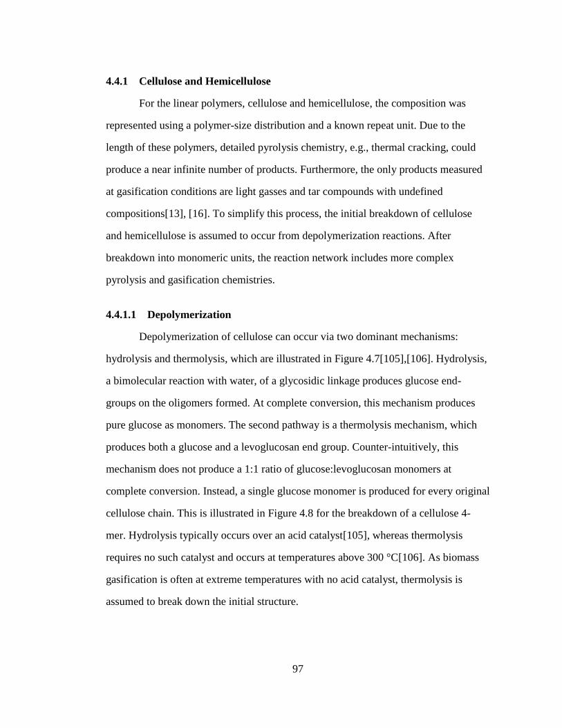
97

4.4.1 Cellulose and Hemicellulose

For the linear polymers, cellulose and hemicellulose, the composition was

represented using a polymer-size distribution and a known repeat unit. Due to the

length of these polymers, detailed pyrolysis chemistry, e.g., thermal cracking, could

produce a near infinite number of products. Furthermore, the only products measured

at gasification conditions are light gasses and tar compounds with undefined

compositions[13], [16]. To simplify this process, the initial breakdown of cellulose

and hemicellulose is assumed to occur from depolymerization reactions. After

breakdown into monomeric units, the reaction network includes more complex

pyrolysis and gasification chemistries.

4.4.1.1 Depolymerization

Depolymerization of cellulose can occur via two dominant mechanisms:

hydrolysis and thermolysis, which are illustrated in Figure 4.7[105],[106]. Hydrolysis,

a bimolecular reaction with water, of a glycosidic linkage produces glucose end-

groups on the oligomers formed. At complete conversion, this mechanism produces

pure glucose as monomers. The second pathway is a thermolysis mechanism, which

produces both a glucose and a levoglucosan end group. Counter-intuitively, this

mechanism does not produce a 1:1 ratio of glucose:levoglucosan monomers at

complete conversion. Instead, a single glucose monomer is produced for every original

cellulose chain. This is illustrated in Figure 4.8 for the breakdown of a cellulose 4-

mer. Hydrolysis typically occurs over an acid catalyst[105], whereas thermolysis

requires no such catalyst and occurs at temperatures above 300 °C[106]. As biomass

gasification is often at extreme temperatures with no acid catalyst, thermolysis is

assumed to break down the initial structure.

98

Hydrolysis, +H2O

Thermolysis

m mer n-m mer

...

n-m merm mer

...

...

...

Figure 4.7: Cellulose Depolymerization Pathways.

2

Figure 4.8: Complete cracking of a cellulose 4-mer showing final monomeric

products.

After breakdown into glucose and levoglucosan, the monomers then undergo

ring opening to form analogous acyclic structures, as shown in Figure 4.9. These

molecules are assumed to be the starting point for more detailed pyrolysis and

gasification chemistry. Full pyrolysis chemistry was not applied on larger or ring-

99

containing molecules as it would add unnecessary detail for species that are not

measured in gasification literature[13], [100], [101].

Figure 4.9: Starting molecules of full cellulose pyrolysis network: linear levoglucosan

(left) and linear glucose (right).

Hemicellulose depolymerization is similar to that for cellulose in that it can

follow both hydrolysis and thermolysis reaction pathways, as shown in Figure 4.10.

Unlike that for cellulose, hemicellulose thermolysis can only occur at end-groups

rather than at any linkage in the molecule. This is due to the nature of the

levoglucosan-like structure, anhydro-xylopyranose, that forms in the thermolysis

reaction. In order to have two five-membered rings in the structure, one of the ether

linkage sites must participate in ring formation. If this were to occur mid-chain, it

would require simultaneous bond-breaking of both ether linkages[98]. Like cellulose,

the final yield of an n-mer breakdown via thermolysis is (n-1) anhydro-xylopyranose

and one xylose.

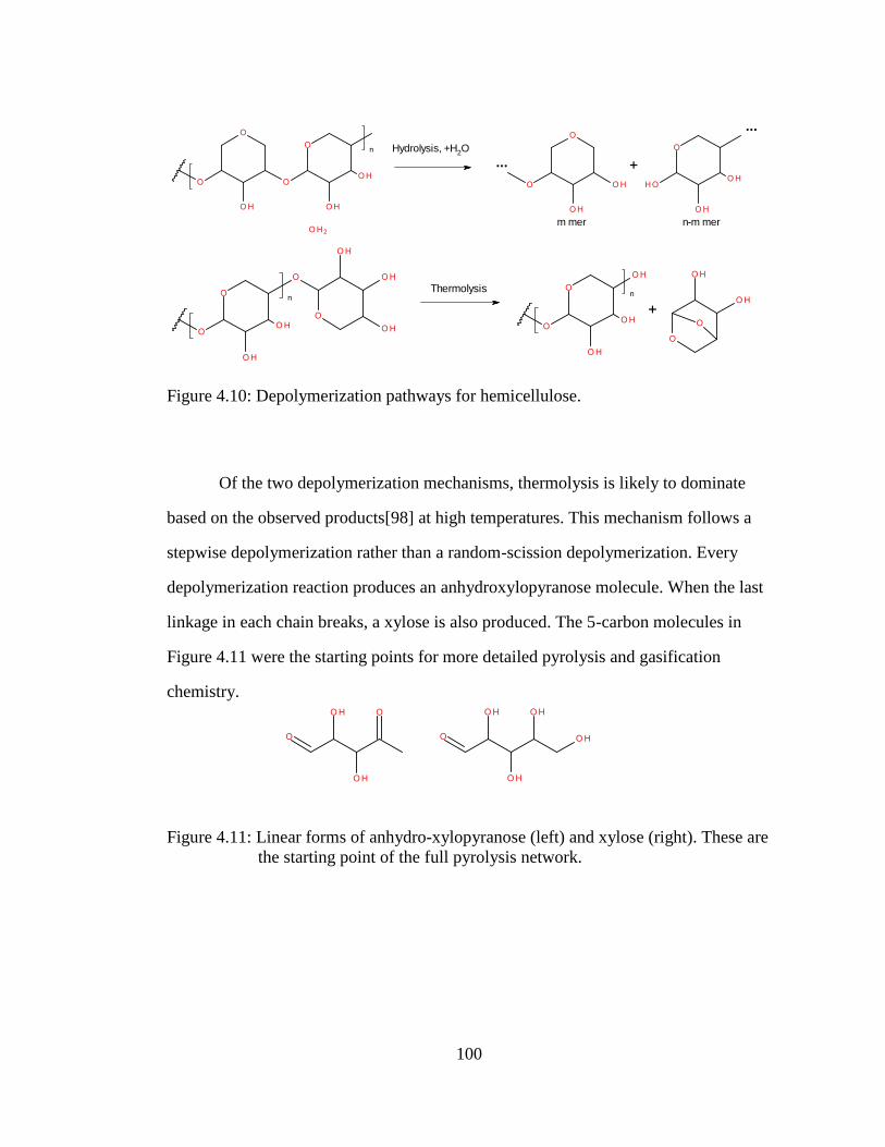
100

n-m mer

...

m mer

...Hydrolysis, +H2O

Thermolysis

Figure 4.10: Depolymerization pathways for hemicellulose.

Of the two depolymerization mechanisms, thermolysis is likely to dominate

based on the observed products[98] at high temperatures. This mechanism follows a

stepwise depolymerization rather than a random-scission depolymerization. Every

depolymerization reaction produces an anhydroxylopyranose molecule. When the last

linkage in each chain breaks, a xylose is also produced. The 5-carbon molecules in

Figure 4.11 were the starting points for more detailed pyrolysis and gasification

chemistry.

Figure 4.11: Linear forms of anhydro-xylopyranose (left) and xylose (right). These are

the starting point of the full pyrolysis network.

101

For both cellulose and hemicellulose, the linear monomers mark the transition

from representing chemical structure using statistics and attributes to representing the

structure using explicit molecules. Within the reaction network, this transition is

represented using the reactions given in Table 4.11.

Table 4.11: Depolymerization reactions representing conversion of attribute

representation to molecular representation for linear polymers.

Hemicellulose Cellulose

𝑯𝒆𝒎𝒊𝒄𝒆𝒍𝒍𝒖𝒍𝒐𝒔𝒆𝑰𝑳𝒕𝒉𝒆𝒓𝒎𝒐𝒍𝒚𝒔𝒊𝒔→

𝑯𝒆𝒎𝒊𝒄𝒆𝒍𝒍𝒖𝒍𝒐𝒔𝒆𝑺𝑪𝟎+𝑯𝒆𝒎𝒊𝒄𝒆𝒍𝒍𝒖𝒍𝒐𝒔𝒆𝑺𝑪𝟏

𝐶𝑒𝑙𝑙𝑢𝑙𝑜𝑠𝑒𝐼𝐿𝑡ℎ𝑒𝑟𝑚𝑜𝑙𝑦𝑠𝑖𝑠→

𝐶𝑒𝑙𝑙𝑢𝑙𝑜𝑠𝑒𝑆𝐶0 + 𝐶𝑒𝑙𝑙𝑢𝑙𝑜𝑠𝑒𝑆𝐶1

𝑯𝒆𝒎𝒊𝒄𝒆𝒍𝒍𝒖𝒍𝒐𝒔𝒆𝒄𝒐𝒓𝒆→ 𝑨𝒏𝒉𝒚𝒅𝒓𝒐𝒙𝒚𝒍𝒐𝒑𝒚𝒓𝒂𝒏𝒐𝒔𝒆

𝐶𝑒𝑙𝑙𝑢𝑙𝑜𝑠𝑒𝑐𝑜𝑟𝑒 → 𝐿𝑖𝑛𝑒𝑎𝑟 𝐿𝑒𝑣𝑜𝑔𝑙𝑢𝑐𝑜𝑠𝑎𝑛

𝑯𝒆𝒎𝒊𝒄𝒆𝒍𝒍𝒖𝒍𝒐𝒔𝒆𝒄𝒐𝒓𝒆→ 𝑳𝒊𝒏𝒆𝒂𝒓 𝒙𝒚𝒍𝒐𝒔𝒆

𝐶𝑒𝑙𝑙𝑢𝑙𝑜𝑠𝑒𝑐𝑜𝑟𝑒 → 𝐿𝑖𝑛𝑒𝑎𝑟 𝑔𝑙𝑢𝑐𝑜𝑠𝑒

The equations for the transition from statistical representation to molecular

representation are based on the mechanism of depolymerization. For hemicellulose,

each link cleavage produces an anhydroxylopyranose due to the unzipping

mechanism. Because there is one reaction site per chain, the rate of unzipping is

proportional to the number of chains in the system. In the last cleavage of each chain,

a linear xylose is also produced. To model this phenomenon, the probability of a linear

xylose forming was set to the ratio of total number of initial hemicellulose chains to

the total number of repeat units. Shorter chain lengths, i.e., larger initial number of

chains, would therefore lead to the production of more linear xylose molecules. These

characteristics yield the rate laws given in Table 4.12.

102

Table 4.12: Depolymerization reaction rate laws representing conversion of attribute

representation to molecular representation for hemicellulose.

Index Reaction Rate Law

1 𝐻𝑒𝑚𝑖𝑐𝑒𝑙𝑙𝑢𝑙𝑜𝑠𝑒𝐼𝐿𝑡ℎ𝑒𝑟𝑚𝑜𝑙𝑦𝑠𝑖𝑠→ 𝐻𝑒𝑚𝑖𝑐𝑒𝑙𝑙𝑢𝑙𝑜𝑠𝑒𝑆𝐶0+ 𝐻𝑒𝑚𝑖𝑐𝑒𝑙𝑙𝑢𝑙𝑜𝑠𝑒𝑆𝐶1

𝑅𝑎𝑡𝑒1 = 𝑘1 ∗ [𝐻𝑒𝑚𝑖𝐶ℎ𝑎𝑖𝑛𝑠]

2 𝐻𝑒𝑚𝑖𝑐𝑒𝑙𝑙𝑢𝑙𝑜𝑠𝑒𝑐𝑜𝑟𝑒→ 𝐴𝑛ℎ𝑦𝑑𝑟𝑜𝑥𝑦𝑙𝑜𝑝𝑦𝑟𝑎𝑛𝑜𝑠𝑒

𝑅𝑎𝑡𝑒2 = 𝑅𝑎𝑡𝑒1

3 𝐻𝑒𝑚𝑖𝑐𝑒𝑙𝑙𝑢𝑙𝑜𝑠𝑒𝑐𝑜𝑟𝑒 → 𝐿𝑖𝑛𝑒𝑎𝑟 𝑥𝑦𝑙𝑜𝑠𝑒

𝑅𝑎𝑡𝑒3 =

𝑅𝑎𝑡𝑒1 ∗[𝐻𝑒𝑚𝑖𝐶ℎ𝑎𝑖𝑛𝑠]0

[𝑇𝑜𝑡𝑎𝑙 𝑅𝑒𝑝𝑒𝑎𝑡 𝑈𝑛𝑖𝑡𝑠]

The mechanism in cellulose depolymerization occurred via random breakdown

in the backbone. This characteristic of depolymerization is analogous to the

assumptions made in a Flory-distributed polymerization; therefore, a Flory distribution

can also be used to model the breakdown. Changes in monomer concentration inform

the production of linear levoglucosan and linear glucose.

The production of monomers from random scission can be related to the

breakdown of the backbone, or d[IL]/dt. First, the number of monomers in a Flory-

distributed polymer as a function of p is given below, in Equation 4.7. The parameter,

N0, corresponds to the number of repeat units in the system, equivalent to the half of

the total sites, as each repeat unit has two sites. Differentiation allows for a

relationship between the change in monomer concentration and dp/dt, shown in

Equation 4.8. The final result, given in Equation 4.9, gives a simple relationship

between increase in monomer concentration and decrease in inter-core linkage

concentration.

𝑁1 = (𝑁0) ∗ (1 − 𝑝)2

𝑤ℎ𝑒𝑟𝑒 𝑁0 =2 ∗ [𝐼𝐿] + [𝑆𝐶]

2

(4.7)

103

𝑑𝑁1𝑑𝑡

= 𝑁0 ∗ −2 ∗ (1 − 𝑝) ∗𝑑𝑝

𝑑𝑡

(4.8)

𝑑𝑝

𝑑𝑡=1

𝑁0∗𝑑[𝐼𝐿]

𝑑𝑡

𝑑𝑁1𝑑𝑡

= −2 ∗ (1 − 𝑝) ∗𝑑[𝐼𝐿]

𝑑𝑡

(4.9)

The increase in monomer concentration is divided into relative increases in

linear levoglucosan and glucose. From the analysis of the depolymerization

mechanism, it was found that a single glucose monomer is produced for every original

chain of cellulose. The probability of forming a glucose repeat unit is proportional to

the total number of chains divided by the number of repeat units given in Equation

4.10. Therefore, if the original system contained shorter polymer chains, then a higher

number of glucose monomers would be produced. These results give the rate laws

shown in Table 4.13.

𝑝𝑟𝑜𝑏𝑔𝑙𝑢 =𝑛𝑢𝑚𝑏𝑒𝑟 𝑜𝑓 𝑜𝑟𝑖𝑔𝑖𝑛𝑎𝑙 𝑐ℎ𝑎𝑖𝑛𝑠

𝑛𝑢𝑚𝑏𝑒𝑟 𝑜𝑓 𝑟𝑒𝑝𝑒𝑎𝑡 𝑢𝑛𝑖𝑡𝑠

𝑝𝑟𝑜𝑏𝑙𝑒𝑣𝑜 = 1 − 𝑝𝑟𝑜𝑏𝑔𝑙𝑢

(4.10)

Table 4.13: Depolymerization reaction rate laws representing conversion of attribute

representation to molecular representation for cellulose.

Reaction Rate Law

𝑪𝒆𝒍𝒍𝒖𝒍𝒐𝒔𝒆𝑰𝑳𝒕𝒉𝒆𝒓𝒎𝒐𝒍𝒚𝒔𝒊𝒔→ 𝑪𝒆𝒍𝒍𝒖𝒍𝒐𝒔𝒆𝑺𝑪𝟎+ 𝑪𝒆𝒍𝒍𝒖𝒍𝒐𝒔𝒆𝑺𝑪𝟏

𝑅𝑎𝑡𝑒1 = 𝑘4 ∗ [𝐶𝑒𝑙𝑙𝑢𝑙𝑜𝑠𝑒𝐼𝐿]

𝑪𝒆𝒍𝒍𝒖𝒍𝒐𝒔𝒆𝒄𝒐𝒓𝒆 → 𝑳𝒊𝒏𝒆𝒂𝒓 𝑳𝒆𝒗𝒐𝒈𝒍𝒖𝒄𝒐𝒔𝒂𝒏 𝑅𝑎𝑡𝑒2 =

𝑑𝑁1𝑑𝑡∗ 𝑝𝑟𝑜𝑏𝑙𝑒𝑣𝑜

𝑪𝒆𝒍𝒍𝒖𝒍𝒐𝒔𝒆𝒄𝒐𝒓𝒆 → 𝑳𝒊𝒏𝒆𝒂𝒓 𝒈𝒍𝒖𝒄𝒐𝒔𝒆 𝑅𝑎𝑡𝑒3 =

𝑑𝑁1𝑑𝑡∗ 𝑝𝑟𝑜𝑏𝑔𝑙𝑢

104

4.4.1.2 Pyrolysis

The pyrolysis reactions in the cellulose and hemicellulose networks serve two

primary purposes: the breakdown into light hydrocarbons and the formation of char,

i.e, stable, heavy molecules. The breakdown of molecules comes in the form of

cracking reactions, as shown below in Table 4.14. The enol-aldehyde tautomerization

is included for two reasons. First, the aldehyde form of the molecule is energetically

more stable. Second, the carbonyl group can undergo decarbonylation, allowing for

further breakdown of the molecule.

105

Table 4.14: Pyrolysis reactions used to breakdown cellulose and hemicellulose into

small molecules.

Reaction Type (Family) and Reactive Moiety

Reaction Matrix



H O C R

H 0 0 -1 1

O 0 0 1 0

C -1 1 0 -1

R 1 0 -1 0

Any aldehyde (primary carbonyl) is allowed to react.

Decarboxylation Carboxylic acids

H O C R

H 0 -1 0 1

O -1 0 1 0

C 0 1 0 -1

R 1 0 -1 0

Any carboxylic acid in the system is allowed to react.

Acyclic Thermal Cracking Hydrocarbon side chains and irreducible molecules

C C C H

C 0 -1 0 1

C -1 0 1 0

C 0 1 0 -1

H 1 0 -1 0

All reactions allowed; however, in cases with multiple reactions for a given site, a single reaction is selected based on radical stability of intermediates as described in the appendix.

Enol-Aldehyde Tautomerization enols

C C O H

C 0 -1 0 1

C -1 0 1 0

O 0 1 0 -1

H 1 0 -1 0

Reaction allowed on any primary enol.

Pyrolysis reactions were also used in the formation of char as summarized in

Table 3.7. The primary reaction family used to create higher molecular weight

molecules was Diels-Alder addition. Other reaction families, e.g. dehydrogenation,

allowed for the formation of stable aromatic molecules such as benzene and

naphthalene.

106

Table 4.15: Pyrolysis reactions used to build aromatic, polyaromatic char molecules.

Reaction Type (Family) and Reactive Moiety

Reaction Matrix



Bimolecular reaction

matrix, more complex

2 and 6 carbon dieneophiles were allowed to react with 4 carbon enes.

Double-bond shift Double bonds

C C C H

C 0 -1 0 1

C -1 0 1 0

C 0 1 0 -1

H 1 0 -1 0

Reactions allowed only on double bonds in a ring.

Dehydrogenation Hydrocarbon side chains and irreducible molecules

C H H C

C 0 -1 0 1

H -1 0 1 0

H 0 1 0 -1

C 1 0 -1 0

Reactions only allowed on cyclic structures.

4.4.1.3 Gasification

Two forms of gasification reactions were included in the cellulose and

hemicellulose networks: incomplete combustion and steam reforming, as shown in

Table 4.16. Gasification reactions between hydrocarbons and hydrogen or CO2, the

other gasifying agents in the MSW gasification process, were assumed to be

negligible. It should be noted that for the included gasification reactions, the rate laws

were assumed to be first order with respect to both reactants. This prevents unrealistic

reaction orders with respect to the gasifying agent.

107

Table 4.16: Gasification reactions in hemicellulose and cellulose networks.

Reaction Type

Example Reaction General Reaction

Incomplete Combustion

3 43.5

𝐶𝑥𝐻𝑦𝑂𝑧 +

𝑥 +𝑦2 − 𝑧

2 𝑂2

→ 𝑥𝐶𝑂 + (𝑦

2)𝐻2𝑂

Steam Reforming

733

𝐶𝑥𝐻𝑦𝑂𝑧 + (𝑥 − 𝑧) 𝐻2𝑂

→ 𝑥𝐶𝑂 + (𝑦

2− (𝑥 − 𝑧))𝐻2

4.4.2 Lignin

4.4.2.1 Interconversion of Attributes

Due to the attribute representation of the composition of lignin, the reaction

network of lignin contains reactions between attributes. In biomass gasification, cores

are modeled to react via gasification reactions to form smaller cores and light gasses.

Side chains and linkages are modeled to react from both pyrolysis and gasification

reactions.

4.4.2.2 Core Reactions

The core reactions currently included in the lignin reaction network are

incomplete combustion and steam reforming. These reactions occur in a stepwise

manner for each of the cores as shown in Figure 4.12. The first core would react with

oxygen or steam to produce a reduced size core. This reduced core would then react

with oxygen or steam to be completely consumed, forming light gases.

The reaction network for cores only included gasification reactions. This was

due to the high thermal stability of cores in the system. The two dominant cores,

accounting for 82 mol% of all cores are benzene and phenol, and they are stable under

108

pyrolysis conditions and are reacted through gasification. Additionally, in cores that

can undergo thermal cracking, the majority of the mass belongs to aromatic rings.

Reactant Core Product Core

Light gas only.

Figure 4.12: Example of stepwise gasification reactions of cores. Each reaction is

written for both incomplete combustion and steam reforming. The

alternate reactions where the phenol ring is gasified first were also

written.

4.4.2.3 Linkage and Side Chain Reactions

The inter-core linkage (IL) and side chain (SC) network contains primarily

cracking, incomplete combustion, and steam reforming reactions. The cracking

reactions are as described in the cellulose and hemicellulose models and include

acyclic thermal cracking and decarbonylation. For side chains, incomplete

combustion and steam reforming reactions were written such that a hydrogen side

chain remained bound to the core as shown in Table 4.17. This characteristic prevents

the product core from having empty binding sites. Similarly, when gasification

reactions occur on inter-core linkages, two side chains must remain to fill the binding

sites on each core.

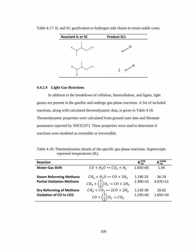
109

Table 4.17: IL and SC gasification to hydrogen side chains to retain stable cores.

Reactant IL or SC Product SCs

4.4.2.4 Light Gas Reactions

In addition to the breakdown of cellulose, hemicellulose, and lignin, light

gasses are present in the gasifier and undergo gas-phase reactions. A list of included

reactions, along with calculated thermodynamic data, is given in Table 4.18.

Thermodynamic properties were calculated from ground state data and Shomate

parameters reported by NIST[107]. These properties were used to determine if

reactions were modeled as reversible or irreversible.

Table 4.18: Thermodynamic details of the specific gas-phase reactions. Superscripts

represent temperatures (K).

Reaction 𝑲𝒆𝒒𝟐𝟗𝟖 𝑲𝒆𝒒

𝟏𝟎𝟎𝟎


1.05E+05 1.44

Steam Reforming Methane 𝐶𝐻4 + 𝐻2𝑂 ↔ 𝐶𝑂 + 3𝐻2 1.19E-25 26.74 Partial Oxidation Methane

𝐶𝐻4 + (1

2)𝑂2 → 𝐶𝑂 + 2𝐻2

1.39E+15 3.07E+11

Dry Reforming of Methane 𝐶𝐻4 + 𝐶𝑂2 ↔ 2𝐶𝑂 + 2𝐻2 1.13E-30 18.62 Oxidation of CO to CO2

𝐶𝑂 + (1

2)𝑂2 → 𝐶𝑂2

1.23E+45 1.65E+10

2

110


The reaction network was generated automatically using in-house software

tools. The pyrolysis networks were generated using the Interactive Network

Generator, or INGen[44],[40]. In this case, three separate networks were generated: a

combined cellulose-hemicellulose network, a lignin core network, and a lignin SC-IL

network. An in-house C# application, INGen Network Merge, was developed to both

merge these networks and add gasification reactions to the system. The final reaction

network features are summarized in Table 3.9. The network contained eight reaction

families for depolymerization and pyrolysis, and six reaction families for gasification

with oxygen and water. The final network contained 1348 reactions and 357 species.

This network was used to construct the kinetic model.

111

Table 4.19: Reaction network diagnostics for the biomass model.

Reaction Families Reactions

Depolymerization and Pyrolysis Acyclic Thermal Cracking

474

Cellulose Depolymerization 3 Double-Bond Shift 76 Decarbonylation 108 Dehydrogenation 10 Diels-Alder 40 Enol-Alde Tautomerization 37 Hemicellulose Depolymerization

3

Gasification Core Oxidation 26 Core Steam Reforming 26 Incomplete Combustion 231 Incomplete Combustion-Chain 55 Steam Reforming 209 Steam Reforming-Chain 45

Light Gas Reactions 5

Total Reactions 1348 Total Species 357

4.6 Model Equations and Kinetics

The model equations in a molecular-level kinetic model are fundamentally a

set of differential equations derived from material balances. The reaction rate

constants are calculated using a standard Arrhenius equation; this gives two rate

parameters, the pre-exponential factor and activation energy, per reaction in the

network.

To reduce the parametric complexity of the model, reaction families and linear

free energy relationships (LFERs) were utilized. First, all reactions from a given

reaction family are modeled to have the same pre-exponential factor. Second, the Bell-

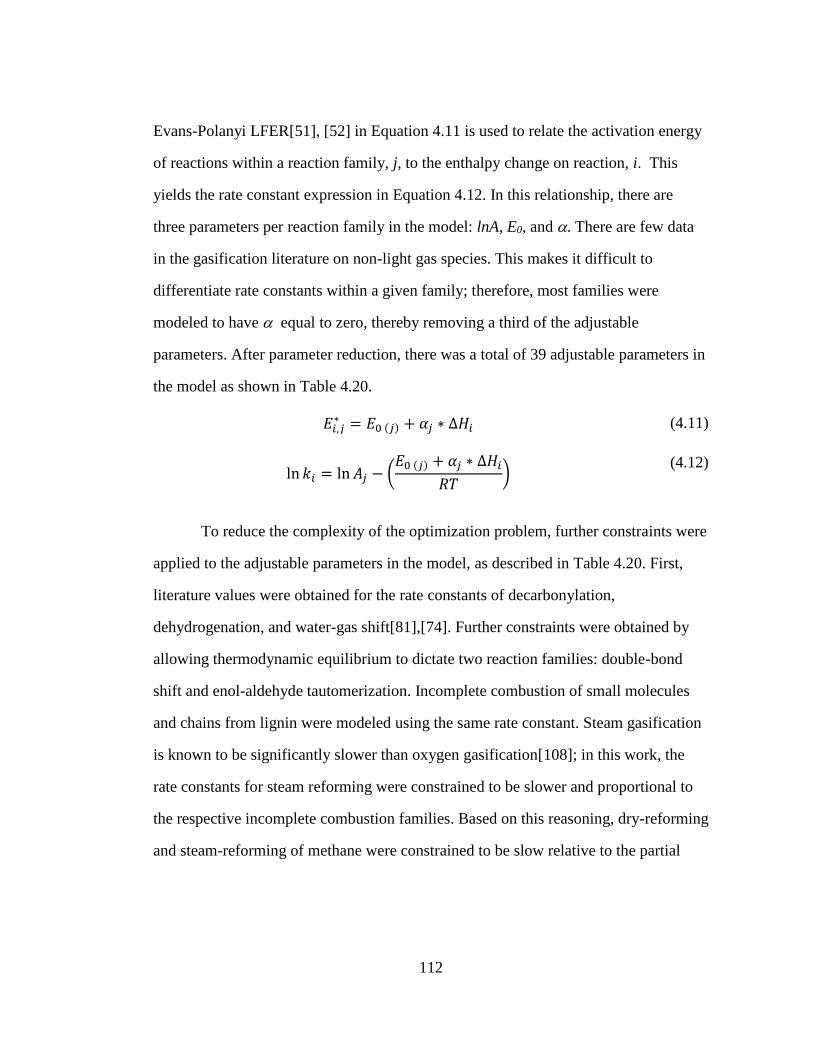
112

Evans-Polanyi LFER[51], [52] in Equation 4.11 is used to relate the activation energy

of reactions within a reaction family, j, to the enthalpy change on reaction, i. This

yields the rate constant expression in Equation 4.12. In this relationship, there are

three parameters per reaction family in the model: lnA, E0, and . There are few data

in the gasification literature on non-light gas species. This makes it difficult to

differentiate rate constants within a given family; therefore, most families were

modeled to have equal to zero, thereby removing a third of the adjustable

parameters. After parameter reduction, there was a total of 39 adjustable parameters in

the model as shown in Table 4.20.

𝐸𝑖,𝑗∗ = 𝐸0 (𝑗) + 𝛼𝑗 ∗ Δ𝐻𝑖

(4.11)


𝑅𝑇)

(4.12)

To reduce the complexity of the optimization problem, further constraints were

applied to the adjustable parameters in the model, as described in Table 4.20. First,

literature values were obtained for the rate constants of decarbonylation,

dehydrogenation, and water-gas shift[81],[74]. Further constraints were obtained by

allowing thermodynamic equilibrium to dictate two reaction families: double-bond

shift and enol-aldehyde tautomerization. Incomplete combustion of small molecules

and chains from lignin were modeled using the same rate constant. Steam gasification

is known to be significantly slower than oxygen gasification[108]; in this work, the

rate constants for steam reforming were constrained to be slower and proportional to

the respective incomplete combustion families. Based on this reasoning, dry-reforming

and steam-reforming of methane were constrained to be slow relative to the partial

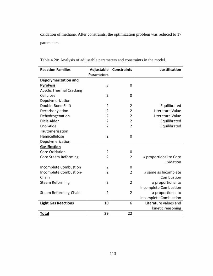
113

oxidation of methane. After constraints, the optimization problem was reduced to 17

parameters.

Table 4.20: Analysis of adjustable parameters and constraints in the model.

Reaction Families Adjustable Parameters

Constraints Justification

Depolymerization and Pyrolysis Acyclic Thermal Cracking

3

0

Cellulose Depolymerization

2 0

Double-Bond Shift 2 2 Equilibrated Decarbonylation 2 2 Literature Value Dehydrogenation 2 2 Literature Value Diels-Alder 2 2 Equilibrated Enol-Alde Tautomerization

2 2 Equilibrated

Hemicellulose Depolymerization

2 0

Gasification Core Oxidation 2 0 Core Steam Reforming 2 2 k proportional to Core

Oxidation Incomplete Combustion 2 0 Incomplete Combustion-Chain

2 2 k same as Incomplete Combustion

Steam Reforming 2 2 k proportional to Incomplete Combustion

Steam Reforming-Chain 2 2 k proportional to Incomplete Combustion

Light Gas Reactions 10 6 Literature values and kinetic reasoning

Total 39 22

114

The material balances for the attribute reaction model used for lignin are in

terms of attributes, rather than species[48], [109]. The equations for the attributes are

analogous to the molecular species material balances and are given below in Equation

4.13. All other traits of the reaction kinetics, e.g. reaction family concept, are

analogous to the irreducible molecule model discussed previously. It should be noted

that despite the attribute representation, the list of molecular species and mole

fractions can be generated at any point in the solution[109]; the attribute material

balances simply change the relative amounts of attributes in the system.

𝑑𝐶𝑜𝑟𝑒̅̅ ̅̅ ̅̅ ̅

𝑑𝑡= ∑ �̅�𝑖 ∗ 𝑟𝑎𝑡𝑒𝑖𝑖, 𝑟𝑒𝑎𝑐𝑡𝑖𝑜𝑛𝑠

(4.13)

a.

𝑑𝐼�̅�


b.

𝑑𝑆𝐶̅̅̅̅


c.


To evaluate the model, literature data from Li et al. on uncatalyzed biomass

gasification in a circulating fluidized bed were simulated. The paper contained data on

five biomass samples and temperatures ranging from 700-815 °C. The reactor was

modeled as a continuous stir tank reactor to simulate the experimental fluidized bed.

The authors performed 15 experiments varying feedstock, temperature, pressure,

oxidation agent, and ash reinjection. The data of primary interest are at atmospheric

pressure with air as the oxidation agent, no ash reinjection, and no added catalyst. For

these runs, the temperature, feedstock, and gas composition are given in Table 4.21.

From this table, runs 3, 4, and 11 were chosen for tuning to test two biomass samples

115

at a moderate range of temperatures. The remaining data sets were reserved to test the

predictive ability of the model.

Table 4.21: Biomass type, temperature, and gas composition for each utilized

experimental run from Li et al (2004). For biomass type, the

abbreviations are Cyp – cypress, hem – hemlock, SPF- spruce, pine, fir.

PS – pine, spruce.

Run Number 2 3 4 11 12 13

Biomass Type cyp. SPF hem. hem. PS mixed

Temperature (°C) 718 766 815 789 701 728

H2 (mol%) 3.1 3.2 3 4.2 5.4 5.1 N2 (mol%) 68.1 67.1 68.4 62.6 53.9 56.3 CO (mol%) 11 10.7 9.6 14.6 21.4 19.9 CH4(mol%) 1.9 1.9 1.9 3 4.6 4.1 CO2(mol%) 15.9 17.1 17.1 15.7 14.7 14.5

The results, in the form of a parity plot, are given below in Figure 4.13.

Tabulated versions of these results are also given in Table 4.22. The results fit well

with experimental data with a best fit line of 𝑦𝑝𝑟𝑒𝑑𝑖𝑐𝑡𝑒𝑑 = 𝑦𝑜𝑏𝑠 ∗ 0.928 + 0.0003.

There are two sources of possible uncertainty. First, there was uncertainty in modeling

the ultimate analysis of the biomass, shown previously in Table 4.10. This was most

notable in the values for oxygen. This can be partly attributed to the absence of sulfur

and nitrogen in the cellulose, hemicellulose, and lignin composition models. Second,

the biomass samples contain varying, trace amounts of ash which can have a catalytic

effect on gasification reactions[110].

116

Table 4.22: Observed and predicted values for data sets in Li et al. All values in the

table are in mol/s.

Composition Data Set 3 (exp, pred)

Data Set 4 (exp, pred)

Data Set 11 (exp, pred)

CH4 0.017, 0.016 0.020, 0.016 0.024, 0.028 H2 0.028, 0.032 0.031, 0.033 0.034, 0.034 CO 0.094, 0.093 0.101, 0.075 0.117, 0.141 CO2 0.150, 0.135 0.179, 0.175 0.126, 0.091

Figure 4.13: Parity plot of tuned data sets for Li et al data. After a linear fit, the

formula comparing experiment to model results is

ypredicted=yobs*0.928+0.0003. The R2 relative to y=x is 0.918 for the tuned

data sets.

In order to test the tuned kinetic parameters, a once-through simulation was run

using all six viable data sets. The parity plot is shown below, in Figure 4.14. The

results are summarized as 𝑦𝑝𝑟𝑒𝑑𝑖𝑐𝑡𝑒𝑑 = 𝑦𝑜𝑏𝑠 ∗ 0.989 − 0.007 even though the

predicted data sets included both a wider temperature range and additional biomass

0.00

0.05

0.10

0.15

0.20

0.25

0.00 0.05 0.10 0.15 0.20 0.25

Pre

dic

ted

val

ues

Observed Values

Data Set 3

Data Set 4

Data Set 11

y=x

117

samples. This suggests model robustness, a key feature for technologies such as MSW

gasification.

Figure 4.14: All viable datasets from Li et al (2004) using tuned parameters from data

sets 3, 4, and 11. Squares represent tuned results, circles are predicted

results. After a linear fit, the formula comparing experiment to model

results is ypredicted=yobs*0.989-0.007. The R2 relative to y=x is 0.861 for

all data sets.

4.8 Tar Prediction and Reaction Family Analysis

A major advantage of molecular-level kinetic models is the ability to ask the

model questions at the molecular level. First, the model predicts both the quantity and

composition of tar, defined here as molecules with a higher boiling point than

benzene. The relative amounts of tar produced in each of the data sets are given below,

in Table 4.23. The trend that data sets 11-13 produced the highest tar agreed with the

experimental measurements[13]. The amount of tar also increases as the biomass/O2

0

0.05

0.1

0.15

0.2

0.25

0.3

0 0.05 0.1 0.15 0.2 0.25

Pre

dic

ted

val

ues

Observed Values

Data Set 3

Data Set 4

Data Set 11

Data Set 2

Data Set 12

Data Set 13

y=x

118

ratio increases as shown in Figure 4.15. The oxygen increase does have a tradeoff in

the quality of the syngas; higher tar fractions had a higher fraction of CO and H2 in

syngas. The composition of tar was predominantly lignin-derived components derived

from benzene and phenol with methoxy substituents. It is important to note that mass

transport, heat transport, and vapor-liquid equilibrium are not taken into account in the

modeling of tar in this model. Any tar molecule that is present in the product stream at

the reactor outlet is considered part of the tar fraction. This is important to note when

comparing with literature studies, such as CPD models by Fletcher and co-

workers[93], [94], that model tar release as well as tar formation. It is not a

fundamental limitation of molecular-level kinetic models to exclude tar release, or

more generally mass and heat transfer effects. An interesting path for future work is to

analyze whether these phenomena play a role in discrepancies between model

predictions and experimental data.

Table 4.23: Weight fraction of tar in output stream for all data sets.

Data Set Tar Fraction

Data Set 2 0.028 Data Set 3 0.031 Data Set 4 0.027 Data Set 11 0.058 Data Set 12 0.058 Data Set 13 0.049

119

Figure 4.15: Tar weight fraction as a function of the ratio of dry biomass to supplied

oxygen (blue, left axis). The fraction of CO and H2 in overall dry syngas

(nitrogen excluded) is also shown (orange, right axis).

The model can also provide additional insight into the process chemistry. First,

during reactor integration, the rates of each reaction are recorded as a function of

reactor volume. The total molar flux through each reaction can then be quantified

using Equation 4.14. For example, if the reaction were the oxidation of CO to CO2, the

summation would return the moles of CO reacted. If the result of Equation 4.14 is

calculated for every reaction within a reaction family, then the total flux through the

reaction family is quantified. A comparison of the relative sums of all reaction

families is given, below, in Figure 4.16. From these results, the dominant pyrolysis

reaction families include the depolymerization of each biomass component. Of the

gasification chemistries, oxidation was far more prevalent than steam reforming.

𝑀𝑜𝑙𝑎𝑟 𝐹𝑙𝑢𝑥 𝑡ℎ𝑟𝑜𝑢𝑔ℎ 𝑟𝑒𝑎𝑐𝑡𝑖𝑜𝑛 = ∑ (𝑉𝑖+1 − 𝑉𝑖) ∗ 𝑟𝑎𝑡𝑒𝑖𝑖, 𝑖𝑛𝑡𝑒𝑔𝑟𝑎𝑡𝑖𝑜𝑛 𝑝𝑜𝑖𝑛𝑡𝑠

(4.14)

0

0.1

0.2

0.3

0.4

0.5

0.6

0.7

0.8

0

0.01

0.02

0.03

0.04

0.05

0.06

0.07

0.08

0 0.5 1 1.5 2 2.5 3

(CO

+H2

)/(C

O+H

2+C

H4+

CO

2)

Tar

Wei

ght

Frac

tio

n

Dry Biomass (kg)/Supplied O2 (kg)

120

Figure 4.16: Relative importance of reaction families in the reactor model integration

for Data Set 11. All analysis was done using an in-house C# application,

KME Results Analyzer.

4.9 Kinetic Rate Constants

The tuned values for the kinetic rate constants relative to Acyclic Thermal

Cracking at 1000K are given in Table 4.24. The initial removal of moisture is

important to gasification processes. Here, this removal is incorporated into the rate

constants for the initial breakdown of polymeric structures. For cellulose and

hemicellulose, the relevant reaction families are cellulose and hemicellulose

depolymerization. For lignin, the primary breakdown of polymeric structure is

cracking, oxidation, and steam reforming of chains.

121

Table 4.24: Rate constants at 1000K relative to Acyclic Thermal Cracking.

log(k)relative,1000=log(k)AcylicThermalCracking,1000-log(k)ReactionFamily,1000. Reaction

families that were assumed to be equilibrated are not included in the

table.

Reaction Family 𝐥𝐨𝐠(𝒌)𝒓𝒆𝒍𝒂𝒕𝒊𝒗𝒆, 𝟏𝟎𝟎𝟎

Depolymerization and Pyrolysis

Acyclic Thermal Cracking 0.00 Cellulose Depolymerization 0.56 Decarbonylation 1.64 Dehydrogenation 0.84 Hemicellulose Depolymerization -3.34 Gasification

Core Oxidation -0.30 Core Steam Reforming -10.62 Incomplete Combustion -2.73 Incomplete Combustion-Chain -2.73 Steam Reforming -5.94 Steam Reforming-Chain -5.94 Light Gas reactions

Water-gas shift -7.46 Oxidation CO to CO2 -2.10 Partial Oxidation of Methane -3.71 Steam Reforming of Methane -5.94 Dry Reforming of Methane -5.94

4.10 Conclusions

This study has demonstrated that the composition of biomass and kinetics of

biomass gasification can be described at the molecular-level. The composition model

showed that individual models for cellulose, hemicellulose, and lignin can be linearly

combined to produce a full biomass composition model that fit well with literature

experimental data. The kinetic model was constructed using a tractable number of

tunable parameters, and was shown to agree not only the data sets used for tuning, but

122

also additional reported results. The results of the kinetic model demonstrated that

syngas composition can be predicted across different biomass samples with the same

set of parameters, thereby addressing a key weakness of lumped kinetic models. This

allows the kinetic model to be used in commercial applications such as municipal solid

waste gasification where the biomass type varies as a function of both time and

location.

123

IMPLEMENTATION OF A MOLECULAR-LEVEL KINETIC MODEL FOR

PLASMA-ARC MUNICIPAL SOLID WASTE GASIFICATION

Scott R. Horton1, Yu Zhang2, Rebecca Mohr2, Francis Petrocelli2, and Michael T. Klein1* 1University of Delaware Energy Institute and Department of Chemical and


Reproduced by permission from Horton, S.R.; Mohr, R.; Zhang, Y.; Petrocelli, F.;

Klein, M.T. “Implementation of a Molecular-level Kinetic Model for Plasma-arc

Municipal Solid Waste Gasification.” (Submitted to Energy & Fuels)

Chapter 5

124

5.1 Abstract

A molecular-level kinetic model was developed for a plasma-arc municipal

solid waste (MSW) gasification unit. The kinetic model included both MSW and

foundry coke. The components included in the MSW kinetic model were biomass and

four common plastics, detailed in earlier reports. The relative amounts of these

components can be optimized for experimental ultimate analyses using an in-house

tool, The MSW Bulk Composition Solver. The reaction chemistries included detailed

pyrolysis and gasification chemistry totaling 1628 reactions and 433 molecular

species. The kinetic model utilized Arrhenius rate laws and contained a material

balance for each species in the model. The model of coke gasification included 10

reactions of surface atoms with oxygen and carbon dioxide. The reaction rates were

modeled using both surface diffusion and intrinsic kinetics. The plasma arc gasifier

was simulated using three zones for MSW: combustion, gasification, and freeboard,

and a separate zone for coke gasification. Each bed was simulated using idealized

chemical reactors with independent conditions. The simulation of the gasifier was

organized in a user-friendly application, organizing measurable inputs and outputs.

This application allowed for trending studies, investigating the effects of equivalence

ratio, MSW composition, and relative sizes of combustion and gasification zones. The

results provided insight into the effects of these variables on tar production, tar

composition, and the quality of produced syngas.

5.2 Introduction

In 2013, the United States produced 250 million tons of municipal solid waste

(MSW)[1]. The management of this waste has evolved over the years, as shown in

Figure 5.1. Historically, MSW was disposed of in landfills; however, in the 1970s,

125

recycling began to become more prevalent. In recent years, the growth of recycling

has tapered off. This begs the question: what should be done with waste that cannot be

economically or efficiently recycled? Currently, landfills remain are the primary

disposal methodology.


material[1].

The economic and environmental issues surrounding landfills motivate waste-

to-energy (WTE) technologies. Environmentally, landfills are potential sources of

groundwater contamination. Also, uncontrolled degradation of waste promotes the

formation of greenhouse gases, such as CH4[111], that are tens of times more potent

than CO2. Economically, WTE is attractive due to landfill tipping fees, energy

recovery, and political incentives. Landfill tipping fees in the US are shown in Figure

5.2, and are currently on the order of 50 USD/ton. Furthermore, these fees are

drastically higher in a more space-limited country; for instance, the UK has tipping

fees of around 120 USD/ton[112]. Also, MSW is a remarkable potential source of

126

energy; it has been estimated that the energy content in only the plastic fraction of US

waste is 700 trillion BTU, equivalent to 139 million barrels of oil, per year[113].

Politically, this energy source has been judged renewable in the UK, and thereby

provides additional revenue from renewable energy credits.

Figure 5.2: Average landfill tipping fees in the US 1982-2013. Prices are in USD.[1]

One of the up-and-comping waste-to-energy technologies is plasma-arc

gasification. This technology offers many advantages over traditional incineration.

First, oxygen is kept lower than stoichiometric levels, thereby reducing the production

of harmful oxygenated pollutants[21]. Second, in gasification the waste is converted to

syngas, a ubiquitous product that can be utilized for electricity or liquid fuel synthesis.

Finally, due to the extreme temperatures in plasma-arc gasification, the final by-

product is a vitrified slag. This slag material passes EPA leech tests and can be utilized

for construction purposes[6].

19.48

49.78

0

10

20

30

40

50

60

1980 1985 1990 1995 2000 2005 2010 2015

Tip

pin

g Fe

e (p

er t

on

, in

flat

ion

ad

j)

127

Models allow for prediction and optimization of reactor outlets for a given

reactor inlet. In the broad sense, plasma arc gasification has three primary inputs:

MSW, Coke, and enriched air. MSW is composed of a variety of components ranging

from paper to food to plastics. Furthermore, the composition of MSW is a function of

both location and time of year. The second inlet, coke, is fed to the reactor as a heat

source and to provide mechanical support for the waste bed. The enriched air stream is

fed at various points along the reactors walls and provides gasification agents for the

breakdown of MSW. A portion of this air inlet is heated by the plasma torch before

entering the main reactor. Interest in modeling MSW gasification stems from the

complexity and variability of these input streams. This variability must be captured for

a useful and robust model of MSW gasification. In particular, the model must predict

response of key outputs, such as syngas and tar composition.

There are many mathematical models of the gasification of MSW, or its

components, in the open literature. The most common type of models are based on

assuming thermodynamic equilibrium[14], [17], [26]–[33] which predict outlet

compositions based only on the temperature of the gasifier. In the outlet composition,

the prediction of tar molecules is important in gasification for downstream processing.

This prediction is problematic for equilibrium models as the extreme temperatures in

the gasifier disallow tar molecules at thermodynamic equilibrium. Therefore, to

predict tar molecules, kinetics are necessary. Xiao et al.[37], used an artificial neural

net to model MSW gasification. Artificial neural nets can predict tar molecules,

however the absence of chemical meaning to connections within the neural net

reduces the insight gained from the model. Zhang and coworkers[34], [35] utilized an

Eulerian model to study the flow characteristics paired with lumped kinetics. Some

128

advantages of lumped kinetics include the model solution time, the number of

equations, and model simplicity. Lumped kinetics have disadvantages in terms of

model robustness if the feed or conditions are perturbed from the data used for

parameter tuning.

In kinetic modeling, the type of model is determined by the complexity of both

the desired inputs to the model and predictions. In this case, the complexity of both

inputs and predictions are at the molecular-level. For instance, a given MSW

composition is a set of molecules and mole fractions, and changes in MSW

composition are reflected in the mole fractions. The predictions of the model, tar and

syngas composition, are also fundamentally represented as a list of molecular

structures and amounts. Because of the molecular nature of model inputs and outputs,

the optimal kinetic modeling approach is also at the molecular-level.

In this work, we have built a molecular-level kinetic model for a plasma-arc

gasifier. For the MSW stream, we have combined models from two prior works on

plastics and biomass gasification[54], [83]. The model of coke gasification, detailed in

this report, takes into account both diffusional and kinetic limitations. The gasifier was

simulated using four zones: combustion, gasification, freeboard, and a coke bed. Each

zone was simulated using an idealized reactor, plug-flow or continuously stirred tank,

with independent reactor conditions. This model was organized using a user-friendly

C# (C sharp) application, allowing for specification of adjustable inputs and rapid

analysis of observable outputs. This app enabled trending studies on important design

parameters.

129

5.3 Kinetic Model Development of Municipal Solid Waste Gasification

The kinetic model of MSW gasification includes biomass and four common

plastics: polyethylene (PE), polyvinyl chloride (PVC), polyethylene terephthalate

(PET), and polystyrene (PS). Kinetic models for biomass and plastic gasification have

been individually discussed in prior publications[54], [83]. These models were

merged for the full model of MSW utilized in this work. In this section, the details of

this model are divided into three categories: the composition model, the reaction

chemistry and reaction network, and the automatically constructed kinetic model.

5.3.1 MSW Composition Model

For molecular-level kinetics, the composition of MSW is a list of molecules

and mole fractions. The composition model takes a lumped input such as MSW, and,

using experimental information, predicts the molecular composition. Model

development was a multistep process. First, the waste components in MSW, shown in

Figure 5.3, were divided into two modeled categories: plastics and biomass-derived.

These two categories were then divided into individual polymers: PE, PVC, PET, PS,

cellulose, hemicellulose, and lignin. The molecular composition model was discussed

for each of these polymers in prior work; however, in general, polymers were

described using known repeat-unit structures and polymer-size distributions. The

molecular composition of MSW was modeled as a weighted average of the polymeric

compositions, where each weighting was based on the fraction of that polymer in

waste.

130

A.

C.

B.

D.

Figure 5.3: MSW Fractions in the United States in 2013. A. Overall fractions as

reported by the EPA. B. MSW divided into four categories. The biomass-

derived category includes food, wood, yard trimmings, textiles, and

paper. The ‘not modeled’ category includes metals, glass, other, and

rubber and leather. C. the cellulose hemicellulose and lignin splits

predicted in prior work[83] using data from Li and coworkers[13]. D.

The relative amounts of included plastics, renormalized from EPA

data[1].

The analysis in Figure 5.3 utilizes literature data for the fractional split of

MSW components, but MSW is an inherently variable feedstock. To allow these

variations, an in-house C# application titled ”MSW Bulk Composition Solver” was

developed for tuning new MSW compositions based on simple experimental ultimate

131

analyses. This application allows the user to vary any of the mass fractions of the

seven polymers. The least-squares objective function of the optimization routine

compares calculated and experimental ultimate analyses. The optimization proceeds

using an in-house simulated annealing algorithm.

Figure 5.4: Screenshot from the MSW Bulk Composition Solver. In this screen, the

checkboxes on the left allow the user to select which fractions are

adjusted during the optimization procedure.

The application in Figure 5.4 allows the user to easily apply ultimate analyses

to the kinetic model; however, it is advised that this cursory experiment only be used

on feedstocks with similar compositions. The optimization problem is underspecified

as there are seven polymers and an ultimate analysis containing only four data points

(C, H, O, Cl). It is better to utilize this application with supplemental information to

reduce the degrees of freedom of the optimization. For instance, relative amounts of

132

individual plastics is known, the optimization problem can be constrained. The impact

of MSW composition on process variables is analyzed in later results.

5.3.2 Reaction Chemistry and Network

The reaction chemistry of MSW gasification includes pyrolysis and

gasification chemistries. Pyrolysis reactions are thermal and take place without the

presence of a gasifying agent, as discussed in prior work[54], [83]. There are two

primary categories of pyrolysis chemistry discussed in Table 5.1. The first category

contains reactions, such as thermal cracking, that break down molecules. The second

type of pyrolysis reactions are based on addition and produce stable tar molecules. A

good example here is Diels-alder addition where a diene reacts with a dienophile to

produce a cyclic olefin.

133

Table 5.1: Pyrolysis reaction families in MSW gasification. These families include

both categories of pyrolysis chemistry: cracking and tar-formation. This

table was adapted from tables in prior work[54], [83].

Reaction Type (Family) and Reactive Moetiy

Example Reaction


Decarboxylation Carboxylic acids Acyclic Thermal Cracking Hydrocarbon side chains and irreducible molecules

Ester Decarboxylation Esters

Ester Rearrangement Esters adjacent to a double bond Enol-Aldehyde Tautomerization enols


Double-bond shift Double bonds

Dehydrogenation Hydrocarbon side chains and irreducible molecules

PET Anhydride Linkage Formation Hydrocarbon side chains and irreducible molecules

134

Gasification reactions take place under the presence of a gasification agent

such as oxygen, water, or carbon dioxide. In this work, the included gasification

reaction families are incomplete combustion and steam reforming, shown below in

Table 5.2; also included in this table are important light-gas reactions such as water-

gas shift.

Table 5.2: Included gasification reactions. Table is directly from Horton et al[54].

Reaction Type Reaction

Incomplete Combustion Example 𝐶3𝐻8 + 3.5𝑂2 → 3𝐶𝑂 + 4𝐻2𝑂

General

𝐶𝑥𝐻𝑦𝑂𝑧 +𝑥 +

𝑦2− 𝑧

2 𝑂2 → 𝑥𝐶𝑂 + (

𝑦

2)𝐻2𝑂

Steam Reforming Example 𝐶3𝐻8 + 3𝐻2𝑂 → 3𝐶𝑂 + 7𝐻2

General

𝐶𝑥𝐻𝑦𝑂𝑧 + (𝑥 − 𝑧) 𝐻2𝑂 → 𝑥𝐶𝑂 + (𝑦

2− (𝑥 − 𝑧))𝐻2


Steam Reforming Methane to CO

𝐶𝐻4 + 𝐻2𝑂 ↔ 𝐶𝑂 + 3𝐻2

Partial Oxidation of Methane

𝐶𝐻4 + (1

2)𝑂2 → 𝐶𝑂 + 2𝐻2

Dry Reforming of Methane

𝐶𝐻4 + 𝐶𝑂2 ↔ 2𝐶𝑂 + 2𝐻2

Oxidation of CO to CO2 𝐶𝑂 + (

1

2)𝑂2 → 𝐶𝑂2

The reaction network for MSW was constructed via merging the networks for

biomass and plastics gasification. Other details of the reaction chemistry can be found

in the original publications[54], [83]. After merging the plastics and biomass

135

networks, the final reaction network for MSW gasification contained 433 species

undergoing 1628 reactions.

5.3.3 Kinetic Model Details

The kinetic model contains a material balance differential equation for each of

the 433 species in the reaction network. When integrating a reactor, these differential

equations are solved simultaneously. The reaction rates are governed using Arrhenius

rate parameters; fundamentally two parameters per reaction. Using the concepts of

linear free energy relationships (LFERs) and reaction families, the number of

adjustable parameters was reduced to three per reaction family[51], [52], [54]. The

values of these parameters were optimized in prior work, and they are left invariant for

simulations shown in the current work.

5.4 Kinetic Model Development of Coke Gasification

5.4.1 Coke Structure and Composition

Coke is co-fed to the MSW gasification unit as a source of heat and

mechanical stability. The particle-size distribution was 4”-6” for the coke in this study.

An ultimate analysis is given in Table 5.3. Elementally, the composition of coke was

almost entirely carbon with trace amounts of hydrogen, sulfur, and nitrogen. Pure

carbon is effectively large sheets of graphene, and therefore the chemical makeup of

this coke is large aromatic clusters. Sulfur and nitrogen are likely contained within the

aromatic rings; and hydrogen is likely exist at edge sites. These compositional details

are key in determining the gasification reactions of coke.

136

Table 5.3: Ultimate analysis of coke fed to the gasifier.

Carbon 98.27

Hydrogen 0.19

Nitrogen 0.96

Sulfur 0.58

5.4.2 Gasification Reactions of Coke

Coke gasification involves between surface atoms and adsorbed gasifying

agents. The surface atoms of coke are carbon, hydrogen, nitrogen, and sulfur. The

dominant gasifying agents are oxygen and carbon dioxide. While hydrogen is

produced and it can react with carbon to form methane, it is not a feed and the reaction

with coke will likely be minimal. Although the surface concentrations of H, N, and S

are low, their gasification reactions are considered to account for their mass.

Simplifications to account for their low concentrations will be discussed.

Carbon can react with oxygen to undergo either complete or incomplete

combustion, as shown in Equation 5.1. There is some debate over the surface

intermediates and exact steps of the mechanisms for this combustion. Walker et al.

gave the mechanism in Equation 5.2 for oxidation where CO originates from carbonyl

surface groups and CO2 originates from lactone surface groups[114]. Later work by

Hurt & Calo proposed mechanism in Equation 5.3 after analyzing experimental data

with a number of rate law options, including a power law, Langmuir-Hinshelwood-

Hougen-Watson, and more complex methods[115]. This mechanism was also the

preferred mechanism in a later work by Feng and Bhatia[116].

𝐶 + (1

2)𝑂2 → 𝐶𝑂

2𝐶 + 𝑂2 → 𝐶𝑂2 (5.1)

137

2𝐶 + 𝑂2 → 2 𝐶(𝑂)

𝐶(𝑂) → 𝐶𝑂

𝐶(2𝑂) → 𝐶𝑂2

(5.2)

2𝐶 + 𝑂2 → 2𝐶(𝑂) 𝐶(𝑂) + 𝑂2 → 𝐶𝑂2 + 𝐶(𝑂) 𝐶(𝑂) → 𝐶𝑂 + 𝐶

(5.3)

The net surface reaction of CO2 with carbon to form CO is shown in Equation

5.4, and was studied by its namesake, Boudouard, in 1905. A proposed mechanism

was developed by Ergun and is given in Equation 5.5[117]. Rate constants for this

mechanism were later studied by Huttinger & Fritz [118]. While more complicated

mechanisms exist, this mechanism was reported to explain most experimental

observations by Feng & Bhatia[116].

𝐶 + 𝐶𝑂2 ↔ 2𝐶𝑂 (5.4)

𝐶 + 𝐶𝑂2 ↔ 𝐶(𝑂) + 𝐶𝑂

𝐶(𝑂) → 𝐶𝑂 + 𝐶 (5.5)

The reactions of nitrogen, sulfur, and hydrogen are less prevalent in the

structure of coke and are less well-studied in literature. Surface nitrogen is in low

percentages and is likely bound to 5- and 6- member aromatic rings in the surface. The

reactions given in Equation 5.6 are proposed by Leppalahti & Koljonen[119] for the

gasification with oxygen and CO2 of surface nitrogen with adjacent surface carbons,

CN. For surface sulfur an analogous mechanism produces COS and is proposed in

Equation 5.7. Finally, for surface hydrogen, the reaction with oxygen is given in

Equation 5.8. For both sulfur and hydrogen, these mechanisms are not based on

literature; however, due to the relative scarcity of these surface atoms, the exact details

of the mechanism is second order in terms of importance.

138

𝑂2 + 𝐶 + 𝐶𝑁 → 𝐶(𝑂) + 𝐶𝑁(𝑂)

𝐶𝑁 + 𝐶𝑁(𝑂) → 𝑁2𝑂 + 2𝐶

𝐶𝑁(𝑂) → 𝑁𝑂 + 𝐶

𝐶𝑁 + 𝐶𝑂2 → 𝐶𝑁(𝑂) + 𝐶𝑂

(5.6)

𝑂2 + 𝐶 + 𝐶𝑆 → 𝐶(𝑂) + 𝐶𝑆(𝑂)

𝐶𝑆(𝑂) → 𝐶𝑂𝑆

𝐶𝑆 + 𝐶𝑂2 → 𝐶𝑆(𝑂) + 𝐶𝑂

(5.7)

2𝐻 + (1

2)𝑂2 → 𝐻2𝑂 (5.8)

5.4.3 Reaction List and Rate Laws

Based on the experimental ultimate and proximate analyses, the coke reaction

network has been simplified from the literature mechanisms, and is shown in Table

5.4. Carbon gasification with oxygen is described using two reactions, producing

either CO or CO2. More complex mechanisms involving surface sites are not utilized

as the system is known to be diffusion-limited at the reactor conditions. Therefore the

combined reaction rate, 𝑟𝑛𝑒𝑡_𝑂2, combines both diffusional limitations and intrinsic

kinetics. The relative production of CO and CO2 is defined using a literature

correlation for the 𝐶𝑂

𝐶𝑂2 (cR) ratio from Arthur[120] and is given in Equation 5.9.

𝑐𝑅 = 2500 ∗ 𝑒−6420𝑇 (𝐾) (5.9)

The rate of consumption of all non-carbon surface elements is assumed to be

proportional to the rate of consumption of carbon. For example, after 10% of the

surface carbon has been consumed, it is assumed that 10% of H, N, S have also been

consumed. These assumptions appear in the rate laws in Table 5.4. Reactions for both

oxygen and carbon dioxide are included as either species can consume carbon. It

139

should be noted that these elements are in small amounts and are not expected to play

a major role in gasifier operation; they were included in this model to close the mass

balance.

140

Table 5.4: Reaction network for the coke gasification model. Definitions: 𝑐𝑅 =𝐶𝑂

𝐶𝑂2 𝑟𝑎𝑡𝑖𝑜, 𝑟𝑛𝑒𝑡 is the net rate taking into account both intrinsic kinetics

and diffusional limitations. [𝐶]0, [𝐻]0, [𝑆]0, [𝑁]0 are the relative initial

amounts of each element in the coke (Units in either Mol/s or Mol/L).

Reaction Rate law

𝑪 + (𝟏

𝟐)𝑶𝟐 → 𝑪𝑶 𝑟1 = 𝑟𝑛𝑒𝑡_𝑂2 ∗

𝑐𝑅

𝑐𝑅+1

𝑪 + 𝑶𝟐 → 𝑪𝑶𝟐 𝑟2 = 𝑟𝑛𝑒𝑡_𝑂2 ∗

1

𝑐𝑅 + 1

𝟐𝑯 + 𝟎. 𝟓𝑶𝟐 → 𝑯𝟐𝑶 𝑟3 = (𝑟𝑛𝑒𝑡_𝑂2 + 𝑟5) ∗

[𝐻]0[𝐶]0

𝑵 + 𝟎. 𝟓𝑶𝟐 → 𝑵𝑶 𝑟4 = (𝑟𝑛𝑒𝑡_𝑂2 + 𝑟5) ∗

[𝑁]0[𝐶]0

𝑪 + 𝑺 + 𝟎. 𝟓𝑶𝟐 → 𝑪𝑶𝑺

𝑟5 = 𝑟𝑛𝑒𝑡_𝑂2 ∗

[𝑆]0[𝐶]0

1 −[𝑆]0[𝐶]0

𝑪 + 𝑪𝑶𝟐 → 𝟐𝑪𝑶 𝑟6 = 𝑟𝑛𝑒𝑡_𝐶𝑂2

𝟐𝑯 + 𝑪𝑶𝟐 → 𝑯𝟐𝑶+ 𝑪𝑶 𝑟7 = (𝑟𝑛𝑒𝑡_𝐶𝑂2 + 𝑟9) ∗

[𝐻]0[𝐶]0

𝑵+ 𝑪𝑶𝟐 → 𝑵𝑶+ 𝑪𝑶 𝑟8 = (𝑟𝑛𝑒𝑡_𝐶𝑂2 + 𝑟9) ∗

[𝑁]0[𝐶]0

𝑪 + 𝑺 + 𝑪𝑶𝟐 → 𝑪𝑶𝑺 + 𝑪𝑶

𝑟9 = 𝑟𝑛𝑒𝑡_𝐶𝑂2 ∗

[𝑆]0[𝐶]0

1 −[𝑆]0[𝐶]0

𝑪𝑶 + (𝟏

𝟐)𝑶𝟐 → 𝑪𝑶𝟐

𝑟10 = 𝑘 ∗ [𝐶𝑂]1.5 ∗ [𝑂2]

0.25 𝑘= 3.16𝐸12

∗ exp(−1.67𝐸8

𝐽𝑘𝑚𝑜𝑙

𝑅𝑇)

5.4.4 Intrinsic Kinetics and Diffusional Limitations

The net rate given in Equation 5.10 of the reaction of carbon with oxygen takes

into account both diffusional limitations and intrinsic kinetics. The Damköhler

141

number, Da, is defined as the ratio of the rate without diffusion limitations over the

diffusion limited rate as shown in 5.11. When Da is small, the reaction rate approaches

intrinsic kinetics, or 𝑟𝑖𝑛𝑡𝑟𝑖𝑛𝑠𝑖𝑐. Similarly, when Da is large, the reaction rate

approaches the diffusion limited rate, or 𝑟𝑑𝑖𝑓𝑓𝑢𝑠𝑖𝑜𝑛𝐿𝑖𝑚𝑖𝑡𝑒𝑑. The intrinsic rate follows an

Arrhenius relationship, given in Equation 5.12.

𝑟𝑛𝑒𝑡_𝑂2 =𝑟𝑖𝑛𝑡𝑟𝑖𝑛𝑠𝑖𝑐1 + 𝐷𝑎

[𝑚𝑜𝑙

𝐿 ∗ 𝑠]

(5.10)

𝐷𝑎 =𝑟𝑖𝑛𝑡𝑟𝑖𝑛𝑠𝑖𝑐

𝑟𝑑𝑖𝑓𝑓𝑢𝑠𝑖𝑜𝑛𝐿𝑖𝑚𝑖𝑡𝑒𝑑

(5.11)

𝑟𝑖𝑛𝑡𝑟𝑖𝑛𝑠𝑖𝑐 = 𝑦[𝑂2] ∗ 𝐴𝑂2,𝐶 ∗ 𝑒−𝐸𝑂2,𝐶𝑅𝑇 [

𝑚𝑜𝑙

𝐿 ∗ 𝑠]

(5.12)

The diffusion limited rate, shown in Equation 5.13, is proportional to the gas

phase oxygen concentration, the surface area to volume ratio of the particle, 𝑆𝐴𝑝

𝑉𝑝, and

the oxygen mass transport coefficient, 𝑘𝑂2. The concentration of oxygen depends on

the temperature, pressure, and oxygen/air feed composition. The surface area to

volume ratio is calculated as a function of time from the initial particle size and the

extent of carbon consumption. The mass transport coefficient is calculated using

Equation 5.14 and involved calculations of the Sherwood, Schmidt, and Reynolds

numbers. The Schmidt number is assumed to be constant as it is a weak function of

temperature and contributes little to the Sherwood number.

𝑟𝑑𝑖𝑓𝑓𝑢𝑠𝑖𝑜𝑛𝐿𝑖𝑚𝑖𝑡𝑒𝑑 = 𝑘𝑂2 ∗ 𝑦[𝑂2] ∗𝑆𝐴𝑝

𝑉𝑝= 𝑘𝑂2 ∗ 𝑦[𝑂2] ∗ (

6

𝑑𝑝) [𝑚𝑜𝑙

𝐿 ∗ 𝑠] (5.13)

142

𝑘𝑂2 =𝑆ℎ ∗ 𝐷𝑂2𝑑𝑝

[𝑚

𝑠] (5.14)

𝑆ℎ = 2.0 + 1.1 ∗ 𝑅𝑒0.66 ∗ 𝑆𝑐0.33

𝑅𝑒 =𝜌𝑔 ∗ 𝑑𝑝 ∗ 𝑣

𝜇

𝑆𝑐 = 0.705

𝐷𝑂2: oxygen diffusivity (m2s-1), 𝑑𝑝: particle diameter (m) 𝑣: bed

velocity of vapor (m/s) 𝜇: viscosity (kg*m-1*s-1), 𝜌𝑔: vapor density (kg*m-3), 𝑆𝐴𝑝: Surface area

of particle (m2) 𝑉𝑝: Volume of particle (m3)

The gasification with CO2 has analogous formulation as both diffusion and

intrinsic rates play a role in determining the kinetics of the reaction. Final equations

are given in Equation 5.15 and Equation 5.16.

𝑟𝑛𝑒𝑡_𝐶𝑂2 =𝑟𝑖𝑛𝑡𝑟𝑖𝑛𝑠𝑖𝑐 ∗ 𝑟𝑑𝑖𝑓𝑓𝑢𝑠𝑖𝑜𝑛𝐿𝑖𝑚𝑖𝑡𝑒𝑑

𝑟𝑖𝑛𝑡𝑟𝑖𝑛𝑠𝑖𝑐 + 𝑟𝑑𝑖𝑓𝑓𝑢𝑠𝑖𝑜𝑛𝐿𝑖𝑚𝑖𝑡𝑒𝑑

(5.15)

𝑟𝑖𝑛𝑡𝑟𝑖𝑛𝑠𝑖𝑐 = 𝑦[𝐶𝑂2] ∗ 𝐴𝐶𝑂2,𝐶 ∗ 𝑒−𝐸𝐶𝑂2,𝐶𝑅𝑇

(5.16)

𝑟𝑑𝑖𝑓𝑓𝑢𝑠𝑖𝑜𝑛𝐿𝑖𝑚𝑖𝑡𝑒𝑑 = 𝑘𝐶𝑂2 ∗ 𝑦[𝐶𝑂2] ∗𝑆𝐴𝑝

𝑉𝑝= 𝑘𝐶𝑂2 ∗ 𝑦[𝐶𝑂2] ∗ (

6

𝑑𝑝)

5.4.5 Analysis of Kinetics in Coke Bed

Diffusional limitation are known to play a role in the gasification of coke at the

reaction temperatures. To examine this idea further, Figure 5.5 shows the values of

𝑟𝑖𝑛𝑡𝑟𝑖𝑛𝑠𝑖𝑐, 𝑟𝑑𝑖𝑓𝑓𝑢𝑠𝑖𝑜𝑛𝐿𝑖𝑚𝑖𝑡𝑒𝑑, and 𝑟𝑛𝑒𝑡_𝑂2 for both 4” and 6” particles at a range of

temperatures. As expected from the equations, the intrinsic rate is independent of

particle size, and the diffusion limited rate decreases with increasing particle size. In

the expected temperature regime of >1400K, diffusion limitations dominate. This is

143

shown in Figure 5.6 which shows the Da as a function of temperature for the two

particle sizes. The temperature region of interest has Da much larger than 1, indicating

surface diffusion control of the rate.

Figure 5.5: Comparison of initial reaction rates for 4” (top) and 6” (bottom) particles

for gasification with oxygen. Data labels give values for diffusion

limitations at 1200K to show comparison in particle sizes.

0

0.05

0.1

0.15

0.2

0.25

1000 1100 1200 1300 1400 1500 1600

Rat

e (

mo

l/(L

*s))

Temperature (K)

intrinsic

diffusion

net

0

0.05

0.1

0.15

0.2

0.25

1000 1100 1200 1300 1400 1500 1600

Rat

e (

mo

l/(L

*s))

Temperature (K)

intrinsic

diffusion

net

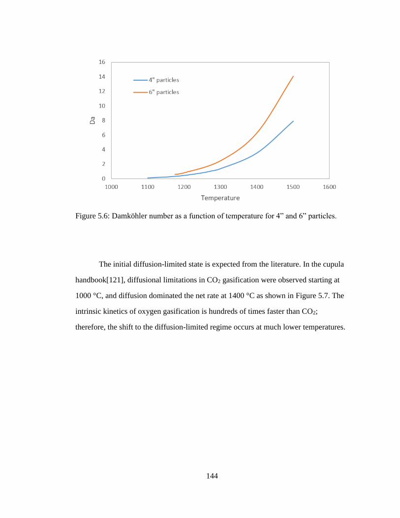
144

Figure 5.6: Damköhler number as a function of temperature for 4” and 6” particles.

The initial diffusion-limited state is expected from the literature. In the cupula

handbook[121], diffusional limitations in CO2 gasification were observed starting at

1000 °C, and diffusion dominated the net rate at 1400 °C as shown in Figure 5.7. The

intrinsic kinetics of oxygen gasification is hundreds of times faster than CO2;

therefore, the shift to the diffusion-limited regime occurs at much lower temperatures.

145

Figure 5.7: Reaction rate contributions as a function of temperature for CO2

gasification from the Cupula Handbook[121]. In the low temperature

region (w1), kinetic limitations dominate. The middle range temperatures,

w2, both kinetics and diffusion contribute to the overall rate. At high

temperatures (w3), diffusional limitations dominate.

5.5 Reactor Simulation of Plasma-arc Gasifier

The coke and MSW gasification kinetic models were used to simulate a 1000

tonne/day gasification facility. To give an idea of the general layout, a diagram of an

Alter Nrg gasifier is given in Figure 5.8[6]. Conceptually, there are four regions of this

reactor: the coke bed, the combustion zone, the gasification zone, and the freeboard

zone.

Figure 5.8: Gasification unit depiction from Young[6] (left) and conceptual

organization of idealized reactors for each reaction zone(right).

146

Each region of the gasifier is modeled as an idealized chemical reactor using

either the MSW or coke gasification models. Design decisions were based on the flow

regimes found in computational fluid dynamic (CFD) simulations performed by APCI

(Air Products and Chemicals Inc.). In the coke bed, the coke is gasified using air or

enriched air. This is a high-temperature bed and is simulated as a plug-flow reactor

using the coke gasification model. The waste inlet is split into both the combustion

and gasification zones. The combustion zone are the regions around air inlets with

high oxygen concentrations and temperatures. The majority of the waste bed is

modeled using the gasification zone which has lower oxygen concentrations and lower

temperatures. Both waste bed zones are modeled as a continuously stirred tank reactor

(CSTR) using the MSW gasification model. The freeboard zone has the largest

volume of any zone and is the region where equilibrium reactions dominate. This zone

is modeled as a plug-flow reactor (PFR) using the MSW gasification model.

5.5.1 MSW Gasification I/O Converter

A user-friendly application was developed to organize and run the model of the

gasification unit. The focus of this application is on measurable inputs and outputs to

the gasification facility. All molecular-level details are abstracted away from the user

and occur in the underlying code. The following discussion details the usage and

features of this application.

The MSW Gasification I/O Converter is shown in Figure 5.9. To use this

application, the user specifies measurable (or known) inputs. Each zone has a volume,

temperature, and pressure; this independence is especially important as there are large

temperature differences across the reactor. The coke bed has additional flow rates for

coke, nitrogen, and oxygen; the independence of the gas flow rates allows for enriched

147

air input. MSW is fed to both the combustion and gasification zones; where the user-

specified 𝛼 determines the mass flow to each zone. Similar to the coke bed, the

combustion zone has independent oxygen and nitrogen flow rates. Moisture is also

taken into account in these zones through two parameters: moisture content of MSW

and relative evaporation volume. The latter term signifies the volume (per kg/hr of

moisture) required for the initial evaporation of moisture within MSW.

Figure 5.9: Screenshot of the main screen from the MSW Gasification I/O Converter.

Measurable process inputs are on the left, the reactor layout is given in

the diagram, and measurable process outputs are on the right.

After clicking the run kinetic model button, each reactor zone is solved to fill

the output tables on the right hand side of Figure 5.9. Due to the linear layout, the

solution is straightforward. The coke bed is solved first, followed by the combustion

zone. These two zones provide inputs to the gasification zone, solved third, which, in

148

turn feeds the freeboard zone, solved last. The initial outputs displayed are syngas

composition and overall tar weight fraction.

There are two key features to this application that are possible due to the

molecular nature of the underlying model. The first is the ability change the

composition of MSW, as shown in Figure 5.10.The tool allows the user to uniquely

specify the fractions of the seven polymers included in MSW, or the user can load a

tuned composition from the MSW Bulk Composition Solver, discussed previously.

The second feature is the ability to analyze the molecular composition of tar

compounds. For each of the MSW beds, the user can perform analysis of the tar

leaving that bed, as shown in Figure 5.11. The form gives a pie chart displaying the

fraction of tar for each dominant species, and the user can view the molecular structure

of each compound.

Perhaps the most important feature of this application is ease-of-use, enabled

by reducing model input and output to measurable quantities. This allows for the user

to quickly test ‘what-if’ scenarios relevant to MSW gasifier operation. For instance,

the effects of MSW composition can be tested in minutes rather than days or weeks.

Furthermore, these tests can be run by anyone from a researcher to an informed

engineer on-site.

149

Figure 5.10: Edit MSW Composition window within the MSW User Friendly

Gasification Model.

Figure 5.11: Tar composition analysis screen in the MSW Gasification I/O Converter.

5.6 Trending Studies

Trending studies of relevant process parameters were completed using the

MSW Gasification I/O Converter. Specifically, the changes in tar flow rate and the

quality of syngas were analyzed as functions of equivalence ratio, MSW composition,

and 𝛼, or the relative flow rate of MSW to the gasification zone. The usage of the

user-friendly application allowed these trending studies to be completed in minutes,

rather than days or weeks.

150

Figure 5.12 shows the effects of the equivalence ratio on the relative flowrates

of tar molecules and the quality of syngas leaving the freeboard zone. As the

equivalence ratio is increased, the relative amount of tar molecules are decreased as

the tar molecules are consumed by oxygen. The quality of syngas also decreases with

increasing oxygen as CO is oxidized to CO2. Over the normal equivalence ratio range

for gasification, 0.3-0.5, the amount of tar and syngas quality decrease by factors of

2.5 and 1.5 respectively. From the point of view of plant engineers, oxygen flow rate

should be set such that tar does not exceed downstream unit specifications; however,

exceeding this flowrate reduces the energy content of the syngas and therefore profits

from electricity production.

151

Figure 5.12: Relative tar fraction and relative syngas quality as a function of

equivalence ratio. The tar fraction is defined as the weight fraction of

species with boiling point greater than or equal to benzene. Syngas

quality here is the mass ratio of CO+H2 to CO+H2+CH4+CO2.

The composition of tar molecules is described using Figure 5.13. The dominant

tar molecules are derived from lignin, benzene, and naphthalene. The aromatic nature

of these tar species is expected from gasification literature of related compounds[21].

The lignin reaction model divided lignin into three types of moieties, cores (ring

structures), inter-core linkages (connections between cores), and side chains (terminal

groups). Most of the mass in lignin tar molecules was contained within benzyl and

phenolic cores. The dominant side chains are methoxy, methyl, and hydroxyl.

Linkages are less prevalent because in the product stream, most linkages have been

0

0.5

1

1.5

2

2.5

3

3.5

4

4.5

5

0.15 0.2 0.25 0.3 0.35 0.4 0.45 0.5 0.55

Tar/

Tar m

in

Syn

gas/

Syn

gas m

in

Equivalence Ratio

Relative Tar Values

Relative Syngas Quality

152

broken from pyrolysis reactions. The remaining linkages are unable to break due to

hydrogen deficiency from cracking and require oxygen for further reaction. If more

oxygen were fed, as in complete combustion, these linkages would break down,

ultimately forming gas phase species.

Figure 5.13: Tar composition leaving the freeboard zone. Left: overall tar molecule

mass fractions. Right: composition of lignin tar molecules.

A molecular-level kinetic model can predict model results for a variable

feedstock. The composition of MSW is variable based on both location and season.

For this trending study, the EPA (US Average) results were compared with two sets of

seasonal data for the UK: winter and summer as shown in Figure 5.14. The

comparisons, given in Table 5.5, show a near constant syngas quality and flow rate for

five different MSW compositions. The tar flow rates increased with increasing

fraction of plastics; although this was a weak function over the range of expected

MSW samples. It should be noted that oxygen flow rates were varied between samples

Lignin-Derived MoleculesBenzeneNaphthaleneOther Tar Molecules

Benzyl Core

Phenol Core

Lignin IL

Lignin SC

153

to hold equivalence ratio constant for the ultimate analyses; this simple experiment

remains the most important for gasifier operation. One difference, not immediately

evident in Table 5.5, between runs is the composition of tars, shown in Figure 5.15. In

this figure, the most extreme cases are compared. In the UK-Summer data set, the tar

are almost entirely lignin-derived molecules, or aromatics with high oxygen content.

Alternatively, if the feed is mostly plastics, the tar is mostly oxygen-free aromatics.

These details are important information for downstream processing.

Figure 5.14: Seasonal Dependence of UK MSW, winter and summer[25].

0

10

20

30

40

50

60

Wei

ght

Per

cen

t

Winter Summer

154

Table 5.5: Comparison of MSW compositions. All data points used equivalence ratio of

0.3. The syngas flow rate was defined as the flow rate sum of CO, CO2, H2,

and CH4. Relative syngas flow rate was the ratio of the flow rate to minimum

flow rate amount the data sets.

Plastics Fraction

Biomass Fraction

Relative Tar

Relative Syngas Quality

Relative Syngas Flowrate

EPA 0.23 0.77 1.27 1.01 1.01 UK - Winter 0.085 0.915 1.07 1.00 1.00 UK - Summer 0.038 0.962 1.00 1.00 1.00 Synthesized 1 0.5 0.5 1.64 1.03 1.03 Synthesized 2 0.8 0.2 1.97 1.03 1.03

Figure 5.15: Comparison of Tar Compositions for different MSW compositions:

Left(UK-Summer), Right(Synthesized 2).

Lignin-Derived Molecules

Benzene

Other Tar Molecules

Lignin-Derived MoleculesBenzeneNapthaleneOther Tar Molecules

155

Figure 5.16: Effect of 𝛼 on relative syngas quality (orange) and tar flow rate (blue) at

equivalence ratios of 0.4 (top) and 0.3 (bottom).

The effects of 𝛼, or the fraction of the MSW bed in the gasification zone, on

relative tar flow rates and syngas quality are given in Figure 5.16. The first

observation is an inverse relationship between syngas quality and tar flow rate. This

observation can be explained as the simulations were run with constant equivalence

ratio, and therefore an increase in tar rate has a corresponding decrease in syngas

quality as CO and H2 are oxidized.

0

0.2

0.4

0.6

0.8

1

1.2

1.4

1.6

1.8

2

0 0.2 0.4 0.6 0.8 1

rela

tive

syn

gas

qu

alit

y re

lati

ve t

ar f

low

rat

e

alpha

0

0.2

0.4

0.6

0.8

1

1.2

1.4

1.6

0 0.2 0.4 0.6 0.8 1

rela

tive

syn

gas

qu

alit

yre

lati

ve t

ar f

low

rat

e

alpha

156

Figure 5.16 also shows a peak in tar flow rate when the fraction of waste

entering the combustion zone is equal to the equivalence ratio, or when 𝛼 = 1.0 − 𝐸𝑅.

The combustion zone is at very high temperature and the waste is completely

combusted to CO2. The peak then aligns with the definition of equivalence ratio, or the

ratio of fuel to O2 required for complete combustion. If the overall process

equivalence ratio is 0.3, and 30% of the MSW is fed to the combustion zone, then the

local equivalence ratio in the combustion zone is 1.0, and the oxygen is completely

consumed. In this scenario, any waste fed to the gasification zone can only be gasified

by H2O, a much slower set of reaction chemistry. Pyrolysis reactions proceed in the

gasification zone, producing tar molecules unabated by incomplete combustion.

The extreme localized temperature in the combustion zone is not beneficial to

gasifier operation provided that waste is also fed to the relatively cooler portions of the

gasification bed. Increasing 𝛼 above the peak value allows oxygen to be in excess in

the combustion zone and reach the gasification bed. Likewise, decreasing 𝛼 below the

peak value, allows a greater portion of the waste to react with oxygen from within the

combustion zone. The lowest tar values and highest syngas quality values are shown

where 𝛼 is zero or one; the scenarios where all waste is present in the same zone as the

O2 feed.

5.7 Summary and Conclusions

A plasma-arc gasifier with simulated for a MSW feedstock using a molecular-

level kinetic model. The two solid inlets to the reactor were MSW and foundry coke.

A molecular-level kinetic model of MSW gasification was developed by combining

models of plastics and biomass gasification. A model of coke gasification with oxygen

and carbon dioxide was developed utilizing both kinetic and diffusional limitations.

157

The gasifier was simulated with a coke bed and three zones for MSW: combustion,

gasification, and freeboard. These models were organized into a user-friendly C#

application called the MSW Gasification I/O Converter. This application prioritized

measurable inputs and outputs, to allow for trending studies on important process

parameters. Some conclusions from this work are:

The coke model was surface-diffusion limited at gasifier conditions.

Increasing equivalence ratio decreases both tar production and

syngas quality. Process optimization is required to maximize profit.

Over normal ranges of waste composition, tar, syngas quality and

syngas flowrate are invariant if equivalence ratio is held constant.

Therefore, ultimate analysis remains an important tool for gasifier

operation. Tar composition requires more in-depth analyses on the

fractions of different waste products.

Tar composition from biomass is primarily aromatics with

methoxy, OH, and methyl side chains; tar composition from

plastics is predominantly benzene and naphthalene.

The localized extreme temperature regions of the combustion zone

can potentially reduce the quality of syngas produced while

increasing the amount of tar exiting the freeboard zone. Tar is

minimized in the well-mixed scenario where all MSW contacts all

oxygen.

Kinetic parameters were optimized (in prior work) to literature data

at much lower temperatures than plasma arc gasification. In the

future, data from gasification facility will allow for trend

verification and the validation and/or improvement of kinetic

parameters.

158

MOLECULAR-LEVEL KINETIC MODELING OF RESID PYROLYSIS

Scott R. Horton1, Linzhou Zhang2, Zhen Hou1, Craig A. Bennett1, Michael T. Klein1, and Suoqi Zhao2 1University of Delaware Energy Institute and Department of Chemical and

Biomolecular Engineering, University of Delaware, Newark, DE 19716 2State Key Laboratory of Heavy Oil Processing, China University of Petroleum,

Beijing 102249, China

Reproduced by permission from Horton, S.R.; Zhang, L.; Hou, Z.; Bennett, C.A.;

Klein, M.T.; Zhao, S. “Molecular-level kinetic modeling of resid pyrolysis” Ind. Eng.

Chem. Res. 2015, 54(16). 10.1021/ie5041572. Copyright 2015. American Chemical

Society.[109]

Chapter 6

159

6.1 Abstract

A molecular-level kinetic model of heavy oil pyrolysis was developed for a

Venezuelan vacuum residue. Model development proceeded in three major steps:

creation of a molecular description of the feedstock, generation of a reaction network,

and model solution and parameter tuning. The feedstock composition, as described in

previous work[46], was modeled in terms of probability density functions (PDFs) of

three finite attribute groups (385 cores, two inter-core linkages, and 194 side chains)

and a PDF for each of a cluster-size and binding site distribution. These attributes, or

molecule building blocks, represent more than 0.4M molecules. An attribute reaction

network was developed using the fundamental reaction chemistry for resid pyrolysis

including 6274 reactions that fall into one of 11 reaction families. To make solution

time tractable, we used Attribute Reaction Modeling (ARM) which constrained the

number of material balances to the number of attributes and irreducible molecules in

the system, or 2841 total equations. Therefore, reactor output was a set of reaction-

altered attribute PDFs and molar amounts of irreducible molecules. The quantitative

molecular composition of the reactor outlet was obtained through the juxtaposition of

the final attribute PDFs. The properties of both the sampled molecules and the char

fraction were obtained using quantitative structure-property relationships (QSPRs).

The kinetic model was tuned using a least-squares objective function comparing the

model predictions to measurements from the molecular to bulk-property level for all

relevant boiling point fractions. The tuned model showed reasonably good agreement

with the experimental measurements.

160

6.2 Introduction

Petroleum is likely to be of primary importance for the coming decades for the

manufacture of liquid fuels. The diminishing supply of conventional, light crude oils

has led to a focus in both industry and academia on heavy oil[122]. Heavy oils pose a

problem as the light fractions of petroleum are easiest to refine into liquid fuels. A

major process to convert heavy oil into lighter fractions is the pyrolysis of vacuum

residue, or resid.

Process models assist in making efficient use of this heavy-oil fraction.

Originally, models of resid were lumped in nature, often phrased in terms of boiling

point cuts[123]. Reactor models therefore contained very few reactions and equations

and were easy to solve and understand. Unfortunately, this simplicity also limits the

usefulness of lumped models as they contain no chemical structure information and

therefore no basis for property estimation beyond the definition of the lump. Two resid

samples with different chemical composition would, therefore, require separate rate

constants. Furthermore, experimental techniques can now identify tens of thousands of

molecular species in a resid sample[124]. By incorporating this detailed information,

the overall efficacy and robustness of reactor models can be increased.

The current state-of-the-art in modeling resid pyrolysis is molecular-level

modeling. These models attempt to capture the full molecular detail of resid. In the

early 1990s, Neurock et al. used Monte Carlo methods to sample 10,000 representative

molecules to model reactions of resid[125]. In 2014, Rueda-Velásquez and Gray[126]

and Oliveira et al.[127] revisited the use of Monte Carlo techniques for thermolysis,

now taking into account modern knowledge of asphaltene composition. Quann and

Jaffe developed structure-oriented lumping (SOL) in order to describe both light and

heavy fractions of petroleum using structural vectors (building blocks)[128]. Recently,

161

delayed coking has been described by Tian and coworkers using the SOL

methodology[129].

While there is extensive literature on resid pyrolysis, no model has

successfully captured the full molecular detail of the reaction of hundreds of thousands

of unique resid molecules because reactor models require a material balance

differential equation for every species. In the coming years, in order to simulate state-

of-the-art experiments, kinetic models must be developed to capture the full molecular

detail of resid. Advances in computational or mathematical algorithms will not

overcome the sheer intractability of these reacting systems; instead, the development

must occur in kinetic modelling approaches.

To address this problem, we will extend previous work[46], [48] that

represented 400,000 resid molecules in terms of probability density functions (PDFs)

of attributes, or building blocks by introducing a novel approach for the kinetics. As

illustrated in Figure 6.1, conventional kinetic modeling would juxtapose the attribute

PDFs before reactor model solution. This results in O(1,000,000), or “on the order of”

1,000,000, material balances and an intractable solution. In this work, we instead

propose to react the attribute PDFs, rather than molecules. This allows for reactor

simulation using only 2839 total material balances. The outlet attribute PDFs are then

juxtaposed to generate the full molecular footprint and associated properties.

162

Figure 6.1: Comparison of Attribute Reaction Modeling and Conventional Modeling

methods.

In the current work, a molecular-level kinetic model was developed and

evaluated for the pyrolysis of a Venezuelan Vacuum Resid. Here, we follow a general

procedure laid out in previous work[46], [48] for model construction. Other details of

the modeling work have been significantly improved over prior work. First, more

detailed reaction chemistries are taken into account. Second, different methods of

attribute juxtaposition have been explored. Finally, this work contains kinetic

parameter tuning to experimental data. The following sections cover each of the major

steps in this process: the molecular representation of the feed, the development of a

163

reaction network, the construction and solution of a kinetic model, and the comparison

of results with experimental measurements.

6.3 Molecular Representation of Resid

Resid is a complex system of molecules, such as the molecule shown in Figure

6.2, where no unique composition defines the feed. Currently, no single analytical

technique provides the identities and amounts of every molecule within a given resid;

therefore composition models must make use of the information available.

Figure 6.2: Example resid molecule and attribute groups: cores (blue), inter-core

linkages (red), and side chains (green).

Conceptually, resid can also be thought of as a collection of structural

moieties, or attributes. Despite the complexity and variability of resid, all possible

molecules are made up of three attribute types: cores, inter-core linkages, and side

chains, as shown in Figure 6.2. Cores are polycyclic molecules containing aromatic

rings and naphthenic rings with or without heteroatoms; inter-core linkages are bridges

between cores; and side chains are terminal substituents bound to cores. The molecular

composition of resid is then a set of probability density functions. First, attribute group

S

S

HO

O

164

pdfs contain information on the relative amount of each attribute. Second, a cluster-

size PDF describes the relative amounts of n-core clusters. Lastly, a binding site PDF

describes the number of filled sites on a given core cluster. This description of resid

allows for the level of model detail to match the level of available experimental

information.

The description of resid as a set of attribute PDFs preserves the molecular-

nature of the composition. The PDFs are juxtaposed, by combining the different

attributes together, to produce a list of molecules. The identity of the molecule is the

combination of the sampled attributes, and the mole fraction is proportional to the

relevant PDF values. For example, the mole fraction calculations of selected

molecules are given below, in Table 6.1.

Table 6.1: The mole fraction calculation for selected molecules from attributes. Pcore,

PIL, and PSC represent the three attribute PDFs. PBS and PCS represent the

binding site and cluster size distributions.

Molecule Attributes Filled

Binding

Sites

Cluster

Size

Mole Fraction

1 1 ∝ 𝑃𝑐𝑜𝑟𝑒 ( )

∗ 𝑃𝑆𝐶( )

∗ 𝑃𝐵𝑆(1) ∗ 𝑃𝐶𝑆(1)

2 2 ∝ 𝑃𝑐𝑜𝑟𝑒 ( )

∗ 𝑃𝑆𝐶( )

∗ 𝑃𝐵𝑆(2) ∗ 𝑃𝐶𝑆(2)

3 2 ∝ 𝑃𝑐𝑜𝑟𝑒 ( )

2

∗ 𝑃𝑆𝐶( )3

∗ 𝑃𝑆𝐶( )

∗ 𝑃𝐵𝑆(3) ∗ 𝑃𝐶𝑆(2)

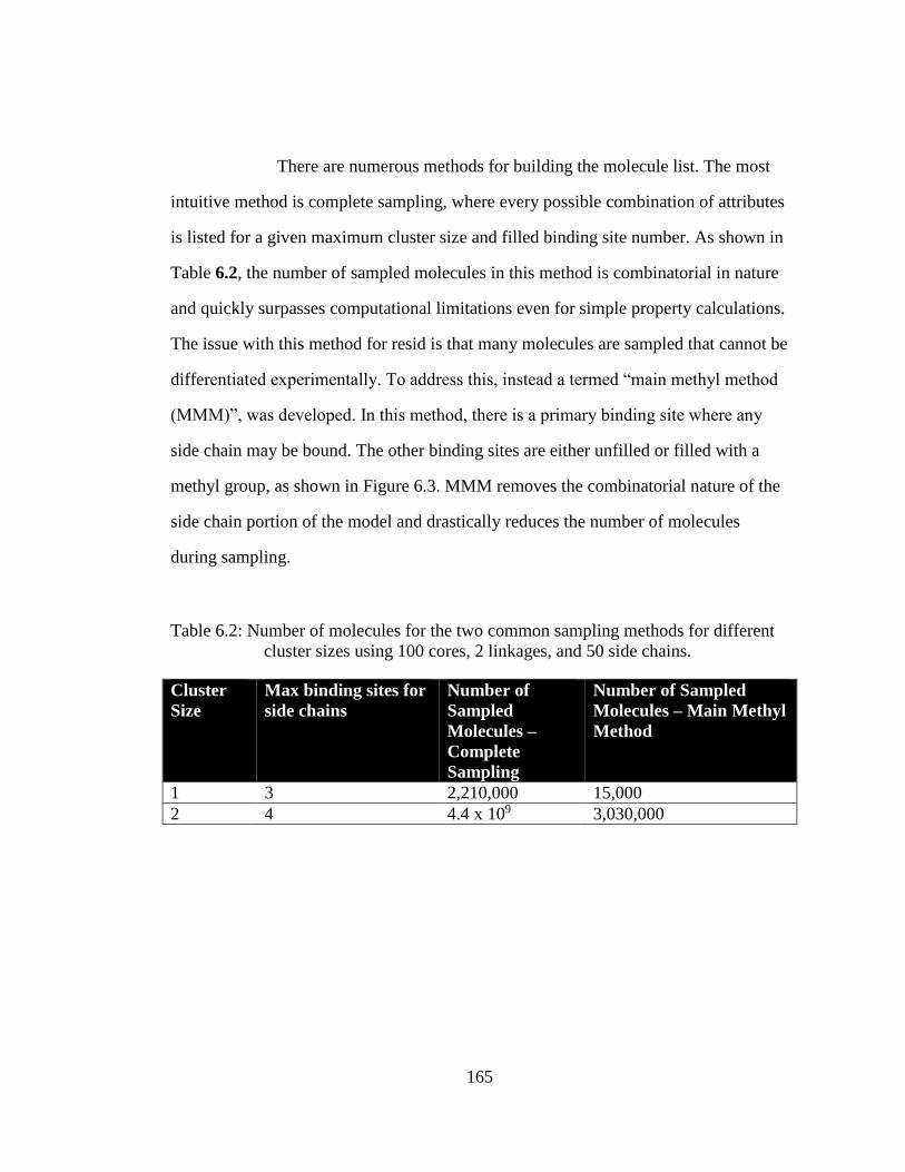
165

There are numerous methods for building the molecule list. The most

intuitive method is complete sampling, where every possible combination of attributes

is listed for a given maximum cluster size and filled binding site number. As shown in

Table 6.2, the number of sampled molecules in this method is combinatorial in nature

and quickly surpasses computational limitations even for simple property calculations.

The issue with this method for resid is that many molecules are sampled that cannot be

differentiated experimentally. To address this, instead a termed “main methyl method

(MMM)”, was developed. In this method, there is a primary binding site where any

side chain may be bound. The other binding sites are either unfilled or filled with a

methyl group, as shown in Figure 6.3. MMM removes the combinatorial nature of the

side chain portion of the model and drastically reduces the number of molecules

during sampling.

Table 6.2: Number of molecules for the two common sampling methods for different

cluster sizes using 100 cores, 2 linkages, and 50 side chains.

Cluster

Size

Max binding sites for

side chains

Number of

Sampled

Molecules –

Complete

Sampling

Number of Sampled

Molecules – Main Methyl

Method

1 3 2,210,000 15,000

2 4 4.4 x 109 3,030,000

166

Complete Sampling R1 and R2 all side chains

Main Methyl Method R1 all side chains, R2 only

methyl

Figure 6.3: Differences in binding sites for complete sampling and main methyl

method.

Further reductions in the sampled molecule list also depend on the available

experimental information. For instance, if the experiment of interest is a distillation

curve which terminates at 750 °C, then there is no need to sample molecules with

boiling points greater than 750 °C. Furthermore, there is no reason to include a higher

level of resolution than the experiment. For instance, if the distillation curve is

accurate to 10 °C, then the cores can be placed into 10 °C lumps. This reduction is

drastic; for instance, if the number of cores was reduced to 50, instead of 100; then the

number of molecules for MMM drops to 7,500 and 765,000 for cluster sizes 1 and 2,

respectively. Through these methods, the molecule list is tailored to remain finite and

representative of the available experimental data.

6.4 Feedstock Composition

The first step in the construction of a molecular-level kinetic model is the

description of the feed at the molecular level. The composition model is described, in

detail, in our previous work[46], where ~600 attributes were used to describe a

molecular composition containing 400,000 molecules after sampling. The first detail

of the composition is the identities of the included attributes. These identities came

from prior knowledge of resid from both literature and experimental data. The 385

167

core attributes included up to nine ring-structures of both naphthenic and aromatic

rings, such as those seen in Figure 6.4. Also included were three heteroatoms: oxygen,

nitrogen, and sulfur. The side chains and inter-core linkages are summarized in Figure

6.5. Four types of side chains were included: n-alkyl, iso-alkyl, sulfide, and carboxylic

acid with up to fifty carbons per side chain type resulting in ~200 total side chains.

There were only two inter-core linkages: a CH2 bridge and a sulfide bridge.

Figure 6.4: Examples of both hydrocarbon and heteroatom-containing core attributes.

Figure 6.5: The four side chain types and two inter-core linkages. The side chain types

are, top-to-bottom, n-alkyl, iso-alkyl, carboxylic acid, and sulfide.

The results of the resid composition model are the three attribute PDFs, a

binding site PDF, and a cluster size PDF. A subset of the three attribute PDFs is given

below in Figure 6.6 and Figure 6.7. The cluster size distribution and binding site

distribution are given in Figure 6.8. In our previous work, these PDFs were sampled to

S

HN

OH O

N

X

XS

X OH

OX

X X

XS

X

168

produce over 400,000 molecules and their associated properties. An example of a

property prediction is a molecular-weight distribution, reproduced below in Figure 6.9.

Figure 6.6: Side chain (left) and Inter-core linkage (right) PDFs. The side chain PDF is

only shown for n-alkyl side chains (normalized to 1). Similar PDFs can

be created for the other side chain types.

0.00

0.05

0.10

0.15

0 20 40 60

Mo

le F

ract

ion

Carbon Number0.0

0.1

0.2

0.3

0.4

0.5

0.6

0.7

Mo

le F

ract

ion

X X XS

X

169

Figure 6.7: Selected cores from the core PDF, mole fractions normalized for the

selected cores.

Figure 6.8: Binding site (left) and cluster size (right) PDFs for feedstock composition.

Results are from model presented by Zhang et al.[46]

0

0.05

0.1

0.15

0.2

0.25

0.3

Mo

le F

ract

ion

OH

SOH

HN

0.0

0.2

0.4

0.6

0.8

1.0

0 1 2 3 4 5

Mo

le F

ract

ion

Number of Filled Binding Sites

0.0

0.2

0.4

0.6

0.8

1.0

1 2 3

Mo

le F

ract

ion

Cluster Size

…

170

Figure 6.9: Molecular weight distribution of the sampled molecules. Figure

reproduced from attribute distributions in Zhang et al[46].

6.5 Reaction Chemistry

Three general reaction types govern resid pyrolysis. First, cracking reactions

reduce the molecular weight of some species and produce small molecules. Second,

aromatization reactions produce hydrogen and lead to stable polycyclic aromatic

hydrocarbons (PAHs). Finally, coking reactions give rise to a high molecular-weight

fraction.

The reaction network applies the process chemistry to the attributes in the

feedstock. For instance, alkyl side chains can crack to small molecules and shorter side

chains. These small molecules can be quantified individually and are therefore termed

irreducible molecules. Examples of irreducible molecules include small paraffins,

olefins, and hydrogen.

The cracking reaction families include decarboxylation, ring-opening, and the

cracking of linear hydrocarbons and C-S bonds. The reaction site and reaction

matrices, along with example reactions, can be found below, in Table 6.3. Reaction

171

rules specify which reaction sites were considered valid sites in reaction network

creation. The rules for cracking were based on the stability of radicals in H-

Abstraction and 𝛽-scission steps. For example, an alkyl side chain on an aromatic ring

has a stable radical at the benzylic position as shown below in Figure 6.10. The two

most favorable scenarios are a benzylic radical after H-abstraction or a benzylic

radical after 𝛽-scission. A full list of reaction rules for the reaction families can be

found in the supplemental information.

Stable after H-

Abstraction

+

Stable After 𝛽-Scission

+

Figure 6.10: Most stable cracking pathways for an alkyl aromatic.

172

Table 6.3: Cracking reaction families, sites, matrices, and examples. These details are

discussed in the PhD Thesis by Zhang[130]. The reaction matrices define

the bond making (1) and bond breaking (-1) in a reaction type.

Reaction Type

(Family) and

Reaction Site


Decarboxylation

Carboxylic acid on

side chain and

irreducible molecules.

H O C C

H 0 -1 0 1

O -1 0 1 0

C 0 1 0 -1

C 1 0 -1 0

Naphthenic Ring

Opening

6-member naphthenic

rings

C C C H

C 0 -1 0 1

C -1 0 1 0

C 0 1 0 -1

H 1 0 -1 0

Sulfide Ring

Opening

5-member sulfide

rings

H C C S

H 0 -1 0 1

C -1 0 1 0

C 0 1 0 -1

S 1 0 -1 0

Thermal Cracking –

Hydrocarbon

Hydrocarbon side

chains and irreducible

molecules

C C C H

C 0 -1 0 1

C -1 0 1 0

C 0 1 0 -1

H 1 0 -1 0

Thermal Cracking –

C-S bonds

Carbon-Sulfur bonds

on side chains and

irreducible molecules

H C C S

H 0 -1 0 1

C -1 0 1 0

C 0 1 0 -1

S 1 0 -1 0

The aromatization reaction families which increase the aromaticity in the

system while releasing hydrogen are given below in Table 6.4. The five reaction

families are based on ring type and number of hydrogen atoms released. Here the rules

were specified such that the number of hydrogens released from a given reaction step

was minimized. For example, an aromatization-2 would take precedence over an

aromatization-4 if a molecule contained both reactive sites.

OH

O

X OH

O

X

+ CO2

+ CO2

SHS

SHS

S HS

X X +

X X +

+

+

+

XS

XSH

XSH

+ H2SX

S SH

SH+ H2S

+

+

173

Table 6.4: Aromatization reaction families, sites, matrices, and examples for

aromatization reactions. These details are discussed in the PhD Thesis by

Zhang[130].

Reaction Type (Family) and Reaction Site


Naphthenic Ring Aromatization-2

C C H H

C 0 1 -1 0

C 1 0 0 -1

H -1 0 0 1

H 0 -1 1 0


C C C C H H H H

C 0 1 0 0 -1 0 0 0

C 1 0 0 0 0 -1 0 0

C 0 0 0 1 0 0 -1 0

C 0 0 1 0 0 0 0 -1

H -1 0 0 0 0 1 0 0

H 0 -1 0 0 1 0 0 0

H 0 0 -1 0 0 0 0 1

H 0 0 0 -1 0 0 1 0


6-carbon, 6-hydrogen analogue to reaction matrix in Naphthenic Ring Aromatization-4.

Sulfide Ring Aromatization-3

Same matrix as Naphthenic Ring Aromatization-2

Sulfide Ring Aromatization-5

Same matrix as Naphthenic Ring Aromatization-4.

The final reaction family is aromatic ring condensation. This reaction allows

for the growth of a char phase. An example is shown below in Figure 6.11. As an

attribute reaction, this can be conceptualized as the formation of a biphenyl inter-core

linkage. Therefore, only one reaction was written for aromatic ring condensation to

represent the possible condensation of any two aromatic cores in the system.

+ H2

+ 2H2

+ 3H2

S S + H2

S S + 2H2

174

Figure 6.11: Aromatic ring condensation example reaction.


With these reaction families and reaction rules, the reaction network was

generated, automatically, using an in-house software, the Interactive Network

Generator, INGen[40], [44]. INGen takes a starting set of reactant molecules as

network building seeds, and exhaustively searches the molecules for the reaction sites.

The addition of the reaction matrix to the reactant sub-matrix gives product molecules.

This is an iterative process as products of reactions can also react. In this case, the

seed molecules were the attributes in resid composition. The final network diagnostics

for the vacuum resid model are given below in Table 6.5.

INGen builds networks very quickly. For instance, the 6,274 reactions here

took ~30 seconds to build on a regular desktop computer (Dell Precision T1500,

Processor: Intel (R) Core i7 [email protected] GHz 2.93 GHz, Memory: 4.00 GB). This

allows network generation to become an iterative process where the user can fine-tune

the network to include the exact level of desired chemical detail. For instance, in this

model, rules were designed for each reaction family.

+

175

Table 6.5: Reaction network diagnostics including total number of reactions,

attributes, and irreducible molecules. These details are discussed in the

PhD Thesis by Zhang[130].

Reaction Family Number of Reactions

Decarboxylation 137

Naphthenic Ring Opening 224

Sulfide Ring Opening 9

Thermal Cracking – Hydrocarbon 3790

Thermal Cracking – C-S bonds 1097

Naphthenic Ring Aromatization-6 8



Sulfide Ring Aromatization-5 9

Sulfide Ring Aromatization-3 6

Aromatic Ring Condensation 1

Total Reactions 6274

Cores 1704

Inter-core Linkages 3

Side-chains 256

Irreducible Molecules 876

6.7 Model Equations

After reaction network construction, a mathematical description of the kinetics

is built to model the reactor. In general, a molecular-level kinetic model is a system of

ordinary differential equations (ODEs) with one material balance per species and an

overall energy balance. In this study, the lab-scale, semi-batch coking reactor that

provided experimental data for comparison was isothermal and therefore only material

balances are relevant. This would equate to O(1,000,000) differential equations in a

conventional kinetic model for resid. Attribute reaction modeling addresses this

intractability while retaining molecular-level detail.

176

First, a balance equation is written for each attribute in the system, as shown in

Equation 6.1. Each equation, written in vector notation, uses 𝜈 to denote stoichiometry

and −𝑟𝑒𝑣𝑎𝑝 to account for the rate of evaporation in the coking semi-batch reactor. In

this model, −𝑟𝑒𝑣𝑎𝑝 was taken into account by restricting slow reaction families on

smaller molecules. For instance, molecules with less than four rings were not allowed

to undergo aromatization. The total number of equations for the attribute portion of

the model is equal to the total sum of the attributes. This trait of the model is

singularly the most important for computational tractability due to the combinatorial

relationship between attributes and molecules. The initial conditions for each attribute

originate from the continuous attribute PDFs from the composition model. The

generation of initial conditions effectively transforms the continuous probability

distributions from the composition into discrete distributions, as illustrated in Figure

6.12.

𝑑𝐶𝑜𝑟𝑒̅̅ ̅̅ ̅̅ ̅

𝑑𝑡= −�̅�𝑒𝑣𝑎𝑝 + ∑ �̅�𝑖 ∗ 𝑟𝑎𝑡𝑒𝑖

𝑖, 𝑟𝑒𝑎𝑐𝑡𝑖𝑜𝑛𝑠

(6.1)

a.

𝑑𝐼�̅�



b.

𝑑𝑆𝐶̅̅̅̅



c.

177

Figure 6.12: Conversion of continuous attribute pdfs to discrete PDFs during the

generation of initial conditions for the reactor kinetic model.

Small molecules that are not reducible into attributes were produced in the

reaction network. A material balance is written for each of these irreducible molecules

as shown in Equation 6.2. The number of irreducible molecules produced is finite, and

the model remains tractable. Combined, the attribute and irreducible molecule material

balances make up the kinetic model. These equations are integrated using the LSODE

suite of differential equation solvers[131].

𝑑𝐼𝑀̅̅ ̅̅



(6.2)

For irreducible molecules, the model solution simply yields molar flows at the

outlet, as in a conventional molecular-level model. For attributes, the integration of the

reactor model alters the relative amounts of attributes in the system. For example, in

Composition Model Results Continuous PDFs

Material Balance Initial Conditions Discrete PDFs

178

the side chain distribution, cracking would increase the amount of methyl (x-CH3) side

chains relative to longer paraffin side chains. Conceptually, model solution can

therefore be represented as the alteration of the discrete attribute PDFs, as shown in

Figure 6.13. The molecular products are obtained via juxtaposition.

Figure 6.13: The alteration of attribute PDFs through model solution.

6.8 Kinetics

The rate constants in the model were followed the standard Arrhenius

expression, given in Equation 6.3. To reduce the parametric complexity, we utilized

the concept that the rates of similar reactions, i.e., members of the same reaction

family, can be correlated. First, all activation energies for a given reaction family, 𝑗,

were constrained using a linear free energy relationship (LFER), such as one posed by

Bell-Evans-Polanyi[51], [52] shown in Equation 6.4. Second, all pre-exponential

factors are assumed to be a function only of reaction family, or ln(𝐴𝑗). The expression

Model Solution

Initial Attribute PDFs Reaction-altered Attribute PDFs

179

for each rate constant in the model, shown in Equation 6.5, is only dependent on

known quantities, temperature and the enthalpy change on reaction (Δ𝐻𝑖), and three

reaction-family dependent parameters (𝐴𝑗, 𝛼𝑗, and 𝐸0 (𝑗)).

ln 𝑘𝑖 = ln𝐴𝑖 −𝐸𝑖∗

𝑅𝑇

(6.3)

𝐸𝑖,𝑗∗ = 𝐸0 (𝑗) + 𝛼𝑗 ∗ Δ𝐻𝑖

(6.4)


𝑅𝑇)

(6.5)

For instances where the data used for tuning do not contain temperature

dependence, the adjustable parameters are reduced to two terms per reaction family.

This is shown in Equation 6.6 as 𝑎𝑗 and 𝑏𝑗. These are the parameters for ten of the

eleven reaction families. For the formation of a biphenyl bond in aromatic ring

condensation, the rate is linearly correlated proportional to the average aromatic

content in the system, as shown in Equation 6.7. There are a total of 21 adjustable

parameters in the model.

ln 𝑘𝑖 = 𝑎𝑗 + 𝑏𝑗 ∗ Δ𝐻𝑖

𝑎𝑗 = ln(𝐴𝑗) −𝐸0 (𝑗)

𝑅𝑇

𝑏𝑗 = −𝛼𝑗

𝑅𝑇

(6.6)

𝑘𝑎𝑟𝑜𝑚𝑎𝑡𝑖𝑐 𝑟𝑖𝑛𝑔 𝑐𝑜𝑛𝑑𝑒𝑛𝑎𝑡𝑖𝑜𝑛 = 𝑎𝑎𝑟𝑜𝑚 ∗ (𝐴𝑣𝑒𝑟𝑎𝑔𝑒 𝐴𝑟𝑜𝑚𝑎𝑡𝑖𝑐 𝐶𝑜𝑛𝑡𝑒𝑛𝑡)

(6.7)


The model was evaluated through comparison of its predictions with the

experimental results given in Table 6.6. Quantitative structure-property relationships,

QSPRs, were used to transform the molecular composition into the higher-level

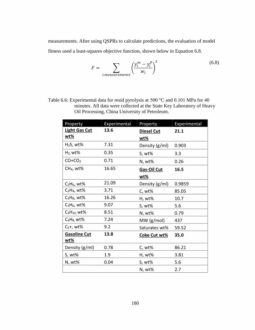
180

measurements. After using QSPRs to calculate predictions, the evaluation of model

fitness used a least-squares objective function, shown below in Equation 6.8.

𝐹 = ∑ (𝑦𝑖𝑚 − 𝑦𝑖

𝑝

𝑤𝑖)

2

𝑖,𝑚𝑒𝑎𝑠𝑢𝑟𝑒𝑚𝑒𝑛𝑡𝑠

(6.8)

Table 6.6: Experimental data for resid pyrolysis at 500 °C and 0.101 MPa for 40

minutes. All data were collected at the State Key Laboratory of Heavy

Oil Processing, China University of Petroleum.

Property Experimental Property Experimental

Light Gas Cut wt%

13.6 Diesel Cut

wt%

21.1

H2S, wt% 7.31 Density (g/ml) 0.903

H2, wt% 0.35 S, wt% 3.3

CO+CO2 0.71 N, wt% 0.26

CH4, wt% 16.65 Gas-Oil Cut

wt%

16.5

C2H6, wt% 21.09 Density (g/ml) 0.9859

C2H4, wt% 3.71 C, wt% 85.05

C3H8, wt% 16.26 H, wt% 10.7

C3H6, wt% 9.07 S, wt% 5.6

C4H10, wt% 8.51 N, wt% 0.79

C4H8, wt% 7.24 MW (g/mol) 437

C5+, wt% 9.2 Saturates wt% 59.52

Gasoline Cut wt%

13.8 Coke Cut wt% 35.0

Density (g/ml) 0.78 C, wt% 86.21

S, wt% 1.9 H, wt% 3.81

N, wt% 0.04 S, wt% 5.6

N, wt% 2.7

181

The weight term, 𝑤𝑖, in the objective function is calculated based on two

sources of standard error. The first is an error incurred by the property measurement.

For instance, there is error in an average molecular weight measurement by GPC. The

second source of uncertainty originates in the structure-property correlation. Some

properties, such as molecular weight, are calculated exactly from a given composition.

Others, such as density, have uncertainty in the structure property correlation. An

analysis of a model’s predictive ability must take into account both types of error. The

total uncertainty, 𝜎𝑡𝑜𝑡𝑎𝑙, for a given data point must then take both 𝜎𝑒𝑥𝑝 and 𝜎𝑄𝑆𝑃𝑅 into

account, as shown in Equation 6.9. The values for 𝜎𝑡𝑜𝑡𝑎𝑙 for the data points are given

below, in

Table 6.7.

𝑤𝑖 = 𝜎𝑖,𝑡𝑜𝑡𝑎𝑙 = √𝜎𝑖,𝑒𝑥𝑝2 + 𝜎𝑖,𝑄𝑆𝑃𝑅

2

(6.9)

182

Table 6.7: Total error and error associated with experiments and quantitative structure

property correlations for the measurements in the objective functions.

Values for error were estimated based on experience in our prior

work[46] with similar data in the objective function.

Property Experiment 𝝈𝒆𝒙𝒑 QSPR 𝝈𝑸𝑺𝑷𝑹 𝝈𝒕𝒐𝒕𝒂𝒍 Boiling Point

Cuts

HT-SimDis 1.2 Group

contribution

Theory

0.05∗ 𝑦𝑜𝑏𝑠

√((0.05∗ 𝑦𝑜𝑏𝑠)

2

+ 0.0122) Light Gas

Composition

Gas Chrom. 0.05∗ 𝑦𝑜𝑏𝑠

Calculated Exactly

0.00 0.05∗ 𝑦𝑜𝑏𝑠

Elemental

Composition

Elemental Analysis


Calculated Exactly

0.00 0.01∗ 𝑦𝑜𝑏𝑠

Density

(g/mol)

Pyncometer 0.00003 Gani Theory



Average

Molecular

Weight

GPC 0.25∗ 𝑦𝑜𝑏𝑠

Calculated Exactly

0.00 0.25∗ 𝑦𝑜𝑏𝑠

SARA SARA Analysis


Calculated Exactly

0.00 0.25∗ 𝑦𝑜𝑏𝑠

After setting up the objective function, the optimization was performed using a

simulated annealing algorithm. The optimization problem was well-posed with over

30 terms in the objective function for 21 adjustable parameters. The parity plot

comparing model and experimental results is given below in Figure 6.14. Included in

this plot are all data points from Table 6.6. These data agreed reasonably well with

experiments with an overall R2 of the parity plot of 0.939. The tuned values for 𝑎𝑗 and

𝑏𝑗 used in predicting this data for each reaction family are given below in Table 6.8.

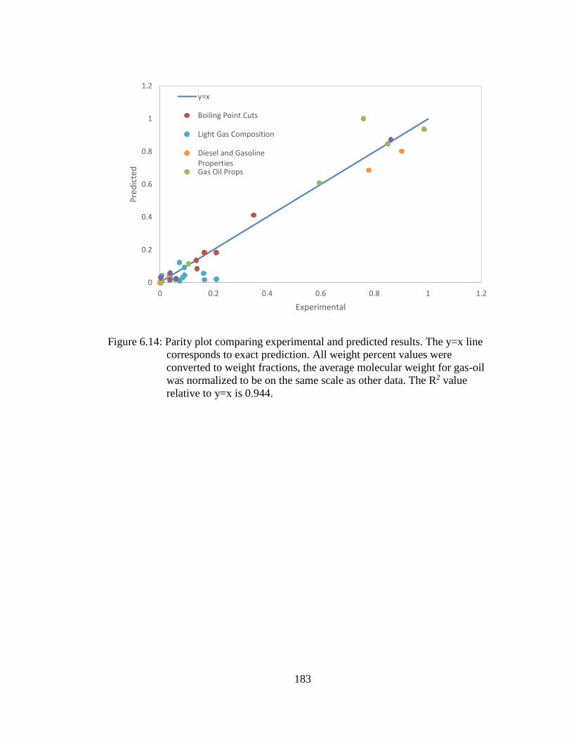
183

Figure 6.14: Parity plot comparing experimental and predicted results. The y=x line

corresponds to exact prediction. All weight percent values were

converted to weight fractions, the average molecular weight for gas-oil

was normalized to be on the same scale as other data. The R2 value

relative to y=x is 0.944.

0

0.2

0.4

0.6

0.8

1

1.2

0 0.2 0.4 0.6 0.8 1 1.2

Pre

dic

ted

Experimental

y=x

Boiling Point Cuts

Light Gas Composition

Diesel and GasolinePropertiesGas Oil Props

184

Table 6.8: Tuned parameters for kinetic model for each reaction family. aj=ln(Aj)-

E0(j)/RT and bj=-αj/RT. For aromatic ring condensation, αj is the scaling

factor, as shown in Equation 6.7. The value for the gas constant used is

R=1.987*10-3 kcal/(mol*K) and T=773 K.

Reaction Family 𝒂𝒋 𝒃𝒋

Decarboxylation 2.041 -0.270

Naphthenic Ring Opening 0.169 -0.275

Sulfide Ring Opening -1.652 -0.301

Thermal Cracking – Hydrocarbon -3.645 -0.150

Thermal Cracking – C-S bonds -3.983 -0.077

Naphthenic Ring Aromatization-6 2.357 -0.255

Naphthenic Ring Aromatization-4 -3.333 -0.278

Naphthenic Ring Aromatization-2 -3.034 -0.112

Sulfide Ring Aromatization-5 -0.006 -0.314

Sulfide Ring Aromatization-3 -1.224 -0.068

Aromatic Ring Condensation 7.800E-05 ------

Figure 6.15: Observed versus experimental including error bars for σtotal; the error bars

were chosen to be drawn on the experimental values. The average

molecular weight for gas-oil was normalized to be on the same scale as

other data.

0

0.2

0.4

0.6

0.8

1

1.2

1.4

Gas

Gas

olin

e

Die

sel

Gas

-Oil

Res

id

Gas

olin

e S

Gas

olin

e N

Die

sel S

Die

sel N

Gas

-Oil

C

Gas

-Oil

H

Gas

-Oil

S

Gas

-Oil

N

Res

id C

Res

id H

Res

id S

Res

id N

Gas

olin

e D

en

sity

Die

sel D

ensi

ty

Gas

-Oil

Den

sity

Gas

-Oil

MW

Gas

-Oil

Satu

rate

s

H₂S H

₂

CO

+ C

O₂

CH

₄

C₂H

₆

C₂H

₄

C₃H

₈

C₃H

₆

C₄H

₁₀

C₄H

₈

C₅+

Observed Experimental

185

The tuned results including 𝜎𝑡𝑜𝑡𝑎𝑙 are given in Figure 6.15 and give more

detailed information on individual experiments than provided by the parity plot. For

instance, the errors in density can be explained by 𝜎𝑡𝑜𝑡𝑎𝑙. The predictions that deviate

from measurements most notably by the model are in the light-gas composition. The

light gas composition is controlled by two reaction families: hydrocarbon cracking and

sulfide cracking. One approximation made is that these two reaction families govern

the cracking of any resid molecule, regardless of boiling point, and it is likely that the

apparent rate constants are different between light gasses and heavy ends. A possible

solution is the inclusion of an additional pair of cracking reaction families for light

gasses. This alternation would only add four parameters to the model. Therefore, the

model would retain its computational tractability. Furthermore, the importance of the

predictive ability of a model for light gasses in resid pyrolysis is minor compared to

other experiments such as boiling point cuts.

The model also predicts molecular level results such as the molecular weight

distribution shown Figure 6.16. When compared to the molecular weight distribution

of the feedstock, the outlet stream is more bimodal with a low molecular weight peak

corresponding to the low boiling point fractions and a higher molecular weight peak

corresponding to coke. The general trend to lower molecular weights correspond to the

cracking of side chains from core molecules. The peaks at low molecular weight

correspond to irreducible molecules. For aromatic ring number, values of all mole

fractions were shifted down due to the production of small molecules. The distribution

was also shifted to higher ring numbers due to aromatic ring condensation and

aromatization. There were relatively fewer naphthenic rings than aromatics in the

186

product due to ring opening reactions. These trends were expected based on the

reaction network and the feedstock.

Figure 6.16: Before (left) and After(right) distributions for MW, aromatic ring

number, and naphthenic ring numbers.

187

6.10 Conclusions

We have shown that a model containing only 2839 equations can simulate the

pyrolysis of O(1,000,000) resid molecules using an Attribute Reaction Model (ARM).

Furthermore, the parametric complexity in the model was reduced to 21 adjustable

parameters using Linear Free Energy Relationships and reaction families. Even with

this reduced number of equations and adjustable parameters, the model agrees well

with experimental data.

The supporting information document contains complete information on the

rules for reaction network construction. This information is available free of charge

via the Internet at http://pubs.acs.org/.

188

ENHANCING THE USER-MODEL INTERFACE THROUGH THE

DEVELOPMENT OF SOFTWARE APPS

For an industrial reactor kinetic model, there are three types of users, given in

Table 7.1. The initial user is the developer of the model. After construction, this model

is subsequently used, understood, and evaluated by research collaborators. Once the

model is in use, the predominant end-user is a process engineer. There are different

goals for the users of kinetic models, yet the common goal is the usage of the model to

predict process outputs from specified or experimentally measured inputs. Research

collaborators and model developers also hope to gain a mathematical and scientific

understanding of the model, model results, and process. Finally, the model developer

hopes to further their kinetic model development capabilities for future projects.

Chapter 7

189

Table 7.1: The types and goals of kinetic model users.

User Type User’s Goals

Model Developer Scientific and mathematical understanding of model and results Usage of model to predict measurable outputs from measurable inputs Furthering kinetic model development capabilities

Research Collaborators Scientific and mathematical understanding of results Usage of model to predict measurable outputs from measurable inputs

Process Engineer Usage of model to predict measurable outputs from measurable inputs

To build the kinetic model, the model developer may use the Kinetic

Modeler’s Toolkit (KMT). There are three software packages within this toolkit, as

shown in Figure 7.1: the Composition Model Editor (CME), the Interactive Network

Generator (INGen), and the Kinetic Model Editor (KME). The starting points of a

kinetic model are experimental data on the feed and reactor outlet, and an

understanding of the process chemistry. CME takes experimental data on the feed to

create a list of molecules and mole fractions of the inlet. INGen utilizes this molecule

list and process chemistry to build a reaction network. Finally, KME uses the reaction

network and feed description to create and solve the equations that define the kinetic

model.

190

Figure 7.1: Main software packages that make up the Kinetic Modeler’s Toolkit

The tools in KMT are designed to be ubiquitous regardless of the kinetic

model; i.e., the same tools are used for MSW gasification as heavy oil resid pyrolysis

or any other process. The strength of these tools therefore lies in the usage by a model

developer. The features of the tools have a very logical progression. When a new

project is started, if the tools do not perform all steps necessary for that project, then

the tools are expanded to match the new project specifications. Over the years of

development, these tools become increasingly more useful to the developers as the

features are expanded to include more experimental measurements, process

chemistries, and reactor configurations. The unfortunate side effect is that the learning

curve for these tools is proportional to the number of features. The tools become less

ideal for many research collaborators and process engineers. These users are only

using a small fraction of overall features in the toolkit and often don’t have the time or

resources to spend on the learning curve.

191

Current expansion of KMT has been in the area of software apps, typically

coded in C# (C-Sharp). The use of the colloquial term ‘app’ implies that these tools

are lightweight in terms of development and use. Each app targets a specific use case

and has one set of features. Alternatively, the larger software suites (CME, INGen, and

KME) were designed to take into account as many use cases and features as possible.

The consequence of the lightweight design approach is that the apps are very fast to

develop, and have an easy learning curve from the point of view of the user. When a

user needs new features, a new app is developed to meet their specific needs; this

leads to many small programs as shown in Table 7.2.

Software apps target the different objectives for the users of kinetic models.

Apps that aim to increase scientific and mathematical understanding focus on

organizing the vast quantities of information produced in a molecular-level kinetic

model. The organized information is primarily displayed via visualization. It is

important to note that these apps retain the molecular information to present to the

user. In contrast, apps that focus on the usage of the model for measured inputs and

outputs abstract all immeasurable information away from the interface. These apps are

typically designed for a specific process and are easy to use regardless of a user’s

background in kinetic modeling. Because of the focus on I/O (inputs/outputs), the apps

are also useful for scenario testing of varying process parameters. The final category

of apps aims to further kinetic model development capabilities. These apps have the

most variety in terms of capability, ranging from the simulation of a particular

experimental reactor to basic flowsheeting capabilities to a properties database.

192

Table 7.2: The categories of apps as organized by objective, corresponding design

method, and a list of apps developed

App Objective App Design Method Apps Developed

Increase scientific and mathematical understanding of the model

Reorganize and visualize information from a molecular-level kinetic model to gain understanding

Reaction Network Visualizer KME Results Analyzer

Usage of the model to predict Measured Outputs from Measured Inputs

Focus on I/O and abstract molecular information away from the user interface.

MSW Gasification I/O Converter Naphtha Reforming I/O Converter

Furthering kinetic model development capabilities

Develop new, lightweight tools to further future kinetic model development.

KME Flowsheet Application TGA Simulator Physical Property Database Interface INGen Network Merge External KME Simulated Annealing CME-Plastics CME-Naphtha MSW Bulk Composition Solver

Most of the C# apps are associated with one or more of the three main software

packages in KMT. A good example is the reaction network visualizer where the main

use case is to visualize and understand INGen networks; the app supports INGen and

assists in the network building process. A second example is the series of I/O

converter apps. These tools effectively utilize CME and KME in a behind-the-scenes

fashion to allow the users to access only the features of CME and KME that are

needed for the project while not being overwhelmed with detail irrelevant to the

project at hand.

193

Table 7.3: The KMT software supported by each App discussed in this thesis.

App Supported KMT Software

CME-Plastics CME

CME-Naphtha CME

MSW-Bulk Composition Solver CME, KME

MSW Gasification I/O Converter KME

Naphtha Reforming I/O Converter CME, KME

Reaction Network Visualizer INGen

Kinetic Results Analyzer KME

KME Flowsheet Application KME

TGA Simulator KME

INGen Network Merge INGen

External KME Simulated Annealing

KME

Physical Property Database Interface

CME, KME

The remainder of this chapter discusses each of the three primary app

objectives from Table 7.2, and explores the functionality of the apps.

7.1 Increasing the Scientific and Mathematical Understanding of the Model

through Apps

Historically, lumped kinetic models had few components and were easy to

understand; however, this came at the cost of scientific rigor as shown in Figure 7.2.

For instance, a lumped kinetic model of coal pyrolysis might contain four lumped

components: coal, tar, volatiles, and char. A few simple plots as a function of

operating conditions contain all of the kinetic data produced by the model, and

therefore the model is easily understood. However, the absolute quantity of

information produced by the model is dwarfed by level of detail actually contained

within the process of coal pyrolysis. The information discrepancy between models and

reality requires many lumped models to describe the realm of possible operating

194

conditions, coal types, etc. Rather than a single, universal description, each lumped

model only contains a small piece of the information that makes up coal pyrolysis.

Figure 7.2: (Left) Typical lumped model of coal pyrolysis. (Right) Conceptual

representation of the information complexity in coal pyrolysis versus

simple lumped models.

Advanced kinetic models are more detailed, but their usefulness is a function

of the user’s ability to comprehend vast quantities of data. The scientific rigor of

modeling has been drastically increased through the advent of advanced experiments,

algorithms, and computing. With increased levels of detail in the model, there is a

better match between the model and what is physically happening within the process.

If a model contained all of the information complexity of coal pyrolysis, then a single,

universal model would suffice for every coal and reactor type. However, the incredible

amount of information in detailed kinetic models shifts the onus of research onto the

user who must understand the model’s equations and results. Unaided, a model can be

difficult to comprehend, reducing the overall scientific usefulness of the results as

shown in Figure 7.3. In order to address the challenge of model comprehension, first

195

we must go into more detail on the information contained within a detailed kinetic

model.

Figure 7.3: Trade-offs of the comprehension and scientific rigor of models as a

function of the number of equations.

Scientific Rigor

Comprehension

Usefulness

Number of Equations

196

Figure 7.4: Information sources and amounts within a molecular-level kinetic model.

Values are relative and qualitative. The relatively low value for rate

parameters is due to a linear free energy relationship (LFER) basis.

The sources and quantities of information in molecular-level kinetics are given

in Figure 7.4. The measured quantities are typically experimental measurements of the

reactor inlets and outlets. Other aspects of the model structure include the reaction

families, reactor type, and rate parameters. Typically, models have far more reactions

than species; resulting in the smaller relative sizes of the molecular (input or output)

compared to the reaction network categories. The largest categories of information are

the reaction rate and molecule profiles within the reactor. Each of these categories

contains a full set of rate and molecule profiles along the reactor length or the reaction

time.

The three main software tools enable the comprehension of many of the

categories of information as described in Table 7.4. For example, CME predicts the

197

molecular input, but it also categorizes the feed using statistical distributions that are

based on molecular structure. INGen helps to organize the reaction network via

categorization into reaction families. There are opportunities for improvement in

understanding the structure of the reaction network. KME also utilizes reaction

families in the area of rate parameters. The most information in the kinetic model and

the biggest issues in comprehension occur after kinetic model solution.

198

Table 7.4: Information types, relevant KMT software, how the information is

organized, and how well the user comprehends the information. *the

comprehension of the reaction network depends on the network size.

Information Type Relevant Software

Method of Organization

Qualitative Comprehension

Property Input CME User-defined and categorized experimental properties

Complete

Molecular Input CME Statistical distributions based on molecular structure

High

Reaction Chemistries

INGen Reaction family list Complete

Reaction Network INGen Organized using reaction families and species

Low-High*

Reactor Type and Conditions

KME User-input. Flow-profile determines reactor type

Complete

Rate Parameters KME User-defined, organized as reaction families

Complete

Reaction Rate Profiles

KME Tabulated, no categorization

Low

Molecular Profiles KME Tabulated, no categorization

Low

Molecular Output KME Tabulated, can be categorized based on user-input

Medium

Property Output KME Experimental properties and bulk properties

Complete

Two C# apps have been developed to target the hardest to comprehend sources

of information in the kinetic model. The Reaction Network Visualizer aims to improve

the understanding of the structure of the reaction network by allowing the user to

199

visualize isolated portions of the network. KME Results Analyzer targets primarily the

rate and molecule profiles in the reactor, but it also helps to address understanding the

molecular-output data.

7.1.1 Reaction Network Visualizer

The reaction network visualizer was developed with the purpose of aiding in

the creation of reaction networks via INGen. It allows for the graphical visualization

of reaction networks, which can aid in viewing the reaction paths from feed molecules

to important product molecules. All trees (or mathematical graphs) are rendered using

the open-source GraphViz software[132].

Figure 7.5: Sample screenshot from the Reaction Network Visualizer. Graph image

rendered using GraphViz[132].

200

Because these networks are too large for easy visualization of the full network,

there are a few smarter methods of using this software. If there is a species of interest,

a user might start from this species with a small number of parent (toward seed3) and

child (toward product) reaction steps. The user can then adjust the numbers to

visualize the desired network. If the graph is obscured by small, common molecules

such as hydrogen or water, the user can elect to remove these molecules from

visualization. Likewise, if a user wishes to focus on particular reaction families, this

can be done as well.

In any scenario, the Reaction Network Visualizer is used to better understand

the reaction network. If the network does contain measured products, then the

Visualizer can be used to help find the unreactive end-points of the network. If the

network is too large and includes too many intermediates, visualization can help

determine the seeds for constrained network building. In order to show the use of this

application for the purpose of constrained network building, ethane pyrolysis is used

as a case study.

Ethane pyrolysis is a well-understood process where radical chemistries are

utilized in models[39], [57]. Because the network is at the mechanistic level, most

radicals in the system can interact with most molecules via H-abstraction reactions

(see Figure 7.6) leading to a network size explosion as rank (reaction steps away from

the network seed, ethane) increases. A qualitative version of this phenomenon is

shown in Figure 7.7. This problem is exacerbated as the product of interest, xylene, is

many reaction steps away from ethane. This detail brings up a quandary: the model is

3 The seeds of the network are the user-specified starting points for reaction network

generation. Often, the seed molecules are synonymous with feed molecules.

201

either finite and useless or infinite and useful. A finite and useful model of ethane

pyrolysis would have xylenes in the finite region of Figure 7.7.

Figure 7.6: Reaction families and some example reactions from ethane pyrolysis. The

primary form of mass increase from ethane is first via olefin addition

reactions. Once large olefins form, Diels-alder additions allow for the

formation of cyclic structures. Beta-scission can then lead to aromaticity

and the product of interest, xylene.

The question then arises: is there a way to lower the rank of xylenes such that

it is in the finite region of model growth? A logical way to model xylene with a finite

number of reactions is by seeding molecules on the path from ethane to xylene. The

reaction network generation can then restrict reactions to remain within a few steps (or

ranks) of the seeded species. This approach is analogous to creating a roadway

between the two molecules, and only allowing for small deviations from that roadway.

2 Initiation: Bond Fission

H-Abstraction

Beta-Scission

Diels-Alder Addition

Olefin Addition

Recombination

202

Determining the molecular identities of these seeds is where network visualization can

play a key role.

Figure 7.7: Number of equations by rank in an ethane pyrolysis model with ethane as

the only seed. The black dots represent the location of xylenes before and

after seeding.

203

Path from ethane to

buta-1,3-diene

Path from buta-1,3-diene

to benzene

Path from buta-1,3-diene to

o-xylene

Figure 7.8: Some major reaction paths visualized using the Reaction Network

Visualizer. Images rendered using GraphViz.

Using the Reaction Network Visualizer, useful seeds for ethane pyrolysis can

be identified as shown in Figure 7.8. The seeds selected are ethene, butadiene,

benzene, and methylcyclohexenes. After reproducing the network, the number of

reactions required to produce o-xylene is drastically reduced as shown in the

204

comparison presented in Table 7.5. This case study shows the utility of the reaction

network visualizer as an aide to generate finite reaction networks.

Table 7.5: Ethane pyrolysis reaction network before and after seeding.

7.1.2 KME Results Analyzer

The KME Results Analyzer was developed for the purpose of gaining

additional understanding of the results produced by KME. This app specifically targets

reactor profile information and the molecular information of the reactor output. For

reactor profile information, the app allows for the user to select specific species in the

output stream and graphically see the reaction families responsible for production and

consumption of the species of interest. For understanding the molecular output, the

app allows the user to specify structural properties (such as aromatic ring class) and

visualize the dominant species that match the constraints. The following text examines

each of these features in greater detail.

Reaction Family Number of Reactions, Only ethane seeded

Number of Reactions, Intermediates seeded

Bond Fission 30 36

H-Abstraction 14,977 2,325

Beta-Scission 325 107

Diels-Alder Addition 4 3

Olefin Addition 17 9

Recombination 153 181

Total Reactions 15,506 2,661

205

Table 7.6: Reaction rate information from KME.

Distance (or time) Reaction 1 Reaction 2 Reaction M

𝒅𝟏 𝑟𝑎𝑡𝑒1(𝑑1) 𝑟𝑎𝑡𝑒2(𝑑1) 𝑟𝑎𝑡𝑒𝑀(𝑑1)

𝒅𝟐 𝑟𝑎𝑡𝑒1(𝑑2) 𝑟𝑎𝑡𝑒2(𝑑2) 𝑟𝑎𝑡𝑒𝑀(𝑑2)

𝒅𝒏 𝑟𝑎𝑡𝑒1(𝑑𝑛) 𝑟𝑎𝑡𝑒2(𝑑𝑛) 𝑟𝑎𝑡𝑒𝑀(𝑑𝑛)

𝑇𝑜𝑡𝑎𝑙 𝑅𝑒𝑎𝑐𝑡𝑖𝑜𝑛 𝑖𝑛𝑡𝑒𝑔𝑟𝑎𝑡𝑖𝑜𝑛 𝑓𝑜𝑟 𝑟𝑒𝑎𝑐𝑡𝑖𝑜𝑛 𝑀

𝑅𝑥𝑛𝐼𝑛𝑡𝑀 = ∑(𝑑𝑖 − 𝑑𝑖−1) ∗ 𝑟𝑎𝑡𝑒𝑀(𝑑𝑖)

𝑛

𝑖=1

, 𝑛𝑜𝑡𝑒 𝑑0 = 0

(7.1)

For profile information, the output of a KME simulation includes the reaction

rates in a tabulated format, as shown in Table 7.6. These values can be integrated

numerically using Equation 7.1. This result tells the user how many moles actually

reacted for each reaction. The reaction integration can help inform a user beyond the

reaction rate parameters. A reaction with a high value of the rate constant will not

show up numerically if there is no reactant present. Similarly, reactions with low rate

constant values might be very important if the reactant concentrations are sufficiently

high. For these reasons, in analyzing the results of a kinetic model, it is useful to

analyze the total integration of the reaction rates throughout the reactor.

In models with reaction families, the adjustable parameters in the model are a

shared pre-exponential factor for the reaction family and the Bells-Evans-Polyani[51],

[52] LFER parameters (slope and intercept) of the activation energy correlation.

Therefore, interest in analyzing a model’s results usually focuses on reaction families

rather than individual reactions. A total reaction family integration can then be found

by summing the total reaction integrations for each member of that family as in

206

Equation 7.2. The results can be displayed graphically in a pie chart that demonstrates

the mathematical significance, on a molar basis, of each reaction family in the system.

For example, the results shown in Figure 7.9 are for naphtha reforming. Key reaction

families here are, as expected, the formation of aromatics from naphthenics, paraffin

cyclization, and isomerization reactions.

𝑅𝑥𝑛𝐹𝑎𝑚𝑖𝑙𝑦𝐼𝑛𝑡𝑃 = ∑ 𝑅𝑥𝑛𝐼𝑛𝑡𝑖

𝑟𝑒𝑎𝑐𝑡𝑖𝑜𝑛𝑠 𝑖𝑛 𝑓𝑎𝑚𝑖𝑙𝑦 𝑝

𝑖=1

(7.2)

Figure 7.9: Full reaction network generation in a Naphtha Reforming model.

In order to understand the reaction rate and species profiles, the analysis of

individual molecular species can yield useful information. For example, the user might

be interested in the reaction families that produce or consume that species.

Mathematically, this is very similar to the full reaction network integration with an

additional term for the stoichiometry, 𝜈, of the species in the reaction, as shown in

207

Equation 7.3. This analysis is represented visually using pie charts, as shown in Figure

7.10. These graphics can help inform which rate parameters are important for the

prediction of the species.

𝑆𝑝𝑒𝑐𝑖𝑒𝑠 𝑅𝑥𝑛𝐹𝑎𝑚𝑖𝑙𝑦𝐼𝑛𝑡𝑃 = ∑ 𝜈𝑖 ∗ 𝑅𝑥𝑛𝐼𝑛𝑡𝑖

𝑟𝑒𝑎𝑐𝑡𝑖𝑜𝑛𝑠 𝑖𝑛 𝑓𝑎𝑚𝑖𝑙𝑦 𝑝

𝑖=1

(7.3)

Figure 7.10: Reaction families responsible for the production of 3-methyldecane.

The full list of species outputs can become overwhelming in large models. To

understand this output, it then becomes helpful to organize the species based on

structural properties. An organization of the species based on structural properties can

provide some better insight to the user. For example, Figure 7.11 shows the eight

carbon i-paraffins in the reactor outlet from a naphtha reforming model. The app also

has the ability to organize the species flowrates using any set of conditional

statements, involving 70 physical properties. For instance, if the user is interested in 1-

208

3 ring aromatic species, then they can specify two conditionals, as shown in Figure

7.12. The app automatically gives the eight most significant species that meet the

specified criteria.

Figure 7.11: Visualization of Bulk Properties in the KME Results Analyzer

209

Figure 7.12: Window allowing the addition of bulk properties to the KME Results

Analyzer. The bulk property added here is 1-3 ring aromatics.

7.2 Enabling the Usage of Model to Predict Measured Outputs from Measured

Inputs

The second category of apps focuses on converting measurable inputs to

measurable outputs. These tools are designed for the full spectrum of users from

Model Developers to Process Engineers. As such, the assumed background of the user

is knowledge of the physical process rather than detailed kinetic modeling. This focus

comes into play in the design of the apps. For instance, technical kinetic vocabulary

such as linear free energy relationships (LFERs) is avoided, while colloquial terms for

experimental measurements are permitted. The apps also minimize user-supplied

information required to run the model. For the kinetic model, the user is allowed to

input process conditions and measurable properties, but not alter the physical process,

equations, or kinetic parameters. The output is customized to suit the user’s needs and

can be a combination of individual species outputs like H2 flow, experimentally

measured bulk properties like PIONA, and reactor conditions like outlet temperature.

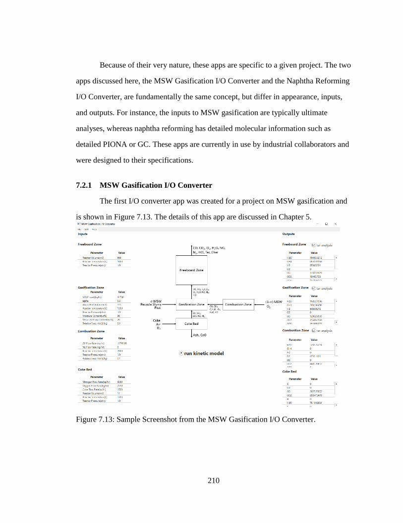
210

Because of their very nature, these apps are specific to a given project. The two

apps discussed here, the MSW Gasification I/O Converter and the Naphtha Reforming

I/O Converter, are fundamentally the same concept, but differ in appearance, inputs,

and outputs. For instance, the inputs to MSW gasification are typically ultimate

analyses, whereas naphtha reforming has detailed molecular information such as

detailed PIONA or GC. These apps are currently in use by industrial collaborators and

were designed to their specifications.

7.2.1 MSW Gasification I/O Converter

The first I/O converter app was created for a project on MSW gasification and

is shown in Figure 7.13. The details of this app are discussed in Chapter 5.

Figure 7.13: Sample Screenshot from the MSW Gasification I/O Converter.

211

7.2.2 Naphtha Reforming I/O Converter

The Naphtha Reforming I/O Converter, shown in Figure 7.14, was developed

to run a detailed kinetic model of a continuous catalytic reforming (CCR) process for

naphtha. The measurable inputs to the model are simulated distillation, carbon number

based PIONA, density, and reactor conditions. The measurable outputs from the

model are light-gas yields, detailed PIONA, and temperature drops across each reactor

bed. Because coking is a key phenomenon in this process, coke formation is also

reported in the output tables.

Behind the scenes, this app runs both a composition model and kinetic model.

In this case, the composition model is a simplified limiting-case of CME

(Composition Model Editor), due to the simplicity of a naphtha feed. The KME model

involves Langmuir-Hinshelwood-Hougen-Watson (LHHW) kinetics on a bifunctional

metal-acid catalyst. Despite this underlying complexity of the kinetic model, the user

simply pastes data into the input table and runs the model by selecting the ‘Run CCR

Model’ button.

A second focus of this app is to enable the blending of feed streams from

different sources. The blender portion of the app allows up to four naphtha feeds. This

is potentially useful in cost-benefit analyses of different crude oils (straight-run

naphtha), or evaluating the effects of feeding naphtha fractions from other refinery

unit outlets such as fluid catalytic cracking (FCC). In the underlying code, the app

simply runs a CME model for each feed stream. The input to the KME model is then

the sum of each of the four feed streams.

212

Figure 7.14: Sample Screenshot from Naphtha Reforming I/O Converter

7.3 Furthering Kinetic Model Development Capabilities

The final category of apps is aimed at furthering the kinetic model

development capabilities of the Kinetic Modeler’s Toolkit (KMT). These apps are

widespread in concept and subject matter. The primary target users of this app are

model developers or specific collaborators.

Three apps are discussed here: KME Flowsheet Application, TGA Simulator,

and the Physical Property Database Interface. The KME Flowsheet Application

provides basic flowsheeting capabilities (e.g., bypass streams) for KME models. TGA

Simulator simulates the thermogravimetric analysis (TGA) experiment using a pre-

213

built KME model. Finally, the Physical Property Database was developed to store

previously calculated properties for tens of thousands of molecules.

Many other apps also fall into the category of furthering development

capabilities and are listed in Table 7.7; detailed explanations of these apps were

excluded from this chapter. For some of these apps, they have been discussed

elsewhere (e.g., MSW Bulk Composition Solver). Others are useful to developers but

are conceptually less significant, such as External KME Simulated Annealing.

Table 7.7: Apps excluded from the current chapter.

App Major Functionality

CME-Plastics (or Plastics Composition Editor) Develop composition models for linear polymers using ultimate analyses as experiments

CME-Naphtha Develop composition models for naphtha feeds (similar to I/O Converter)

MSW-Bulk Composition Solver Predict polymer fractions in waste from ultimate analysis, detailed in chapter XX (REFERENCE)

INGen Network Merge Merge INGen models, modify reaction network to include gasification reactions, detailed in chapter XX (REFERENCE)

External KME Simulated Annealing Run simulated annealing as a separate application from Excel and allow for visualization of tuning progress and frequent backup of parameters

214

7.3.1 KME Flowsheet Application

The KME Flowsheet Application, shown in Figure 7.15, was built to

incorporate basic flowsheeting capabilities into the Kinetic Modeler’s Toolkit (KMT).

The strength of the flowsheet app is the reactor block, which incorporate molecular-

level kinetics from KME. The advantage this application has over traditional KME is

primarily in the ability to split streams and perform reactor bypasses. This is shown in

the diagram in Figure 7.15. The Sep1 block is a basic splitter that was added to allow

for bypass streams. Finally, heaters were added for reactor models, such as naphtha

reforming, where energy balances play a key role in cost analyses.

Figure 7.15: Sample screenshot from the KME Flowsheet Application. The flowsheet

layout images in the KME Flowsheet Application are rendered using the

open-source GraphViz software[132].

215

A full list of block types and descriptions are given in Table 7.8. Three reactors

were included in the flowsheet: PFR, CSTR, and CCR. Of these reactors, CCR

requires further explanation. In CCR, there is cross-directional flow of the catalyst and

reactant stream. The catalyst flow is much slower than the reactant flow, and therefore

the solution is treated as a set of separable ordinary differential equations within KME.

In the future, as KME is updated to include more reactor types, the flowsheet will also

be updated to include these reactors. For separation, there are three included

separators. The simple splitter effectively splits the entire stream evenly; the mole

fractions and species within product streams are the same as the inlet stream. The

specific splitter allows for the split of each molecular species to be uniquely specified.

Finally, the flash allows for a basic temperature-based split, without vapor-liquid

equilibrium (VLE) calculations. The final unit is a heater that calculates heat duty for a

given outlet stream temperature.

216

Table 7.8: Block Types and Descriptions included in KME Flowsheet Application.

Block Type Description

Reactor Block housing a kinetic model from KME

PFR Plug-flow reactor

CSTR Continuously stirred tank reactor

CCR Continuous Catalytic Reformer

Separator Block allowing for stream separation

Simple Splitter Split entire stream on a molar basis, with split governed by a single parameter

Specific Splitter User-defined molar separation for every species, with n-parameters for n species

Flash Split based on boiling temperature assuming perfect split with no VLE calculations performed

Heater Calculate heat required for stream temperature change using a molar-averaged heat capacity of all species in the stream

Solution of a KME Flowsheet Application follows a sequential order. The

solution rank is determined automatically by representing the flowsheet as a

mathematical graph. Each block is given a solution rank based on its proximity to a

process input. For instance, the example flowsheet from Figure 7.15 has solution

orders listed in Figure 7.16. If there are loops (i.e., recycle streams), then the current

version of this app does not allow for solution. The inclusion of recycles requires

iterative solutions and will be included in future versions of this app.

217

Figure 7.16: Solution order of blocks in the example flowsheet.

7.3.2 TGA Simulator

Thermogravimetric analysis (TGA) is a common lab-scale experiment found in

the literature[58], [60], [63], [77], [94], [133]. The technique is ubiquitous and has

been applied to feedstocks ranging from biomass to coal to plastics. As shown in

Figure 7.17, TGA is a technique where a given mass of a compound, such as coal or

biomass, is heated at a constant rate and the mass loss is measured. The vapor phase is

either continually vented or quantified using a gas chromatograph. Mass loss occurs

from two sources: first, as temperature increases, increasingly heavier components

boil and enter the vapor phase; second, pyrolytic and gasification (if air inlet) reactions

break down large molecules into lighter molecules with lower boiling points.

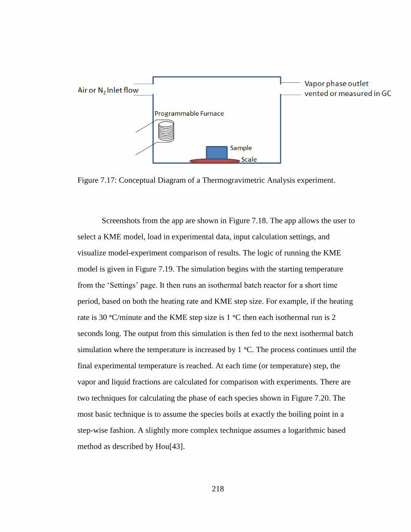
218

Figure 7.17: Conceptual Diagram of a Thermogravimetric Analysis experiment.

Screenshots from the app are shown in Figure 7.18. The app allows the user to

select a KME model, load in experimental data, input calculation settings, and

visualize model-experiment comparison of results. The logic of running the KME

model is given in Figure 7.19. The simulation begins with the starting temperature

from the ‘Settings’ page. It then runs an isothermal batch reactor for a short time

period, based on both the heating rate and KME step size. For example, if the heating

rate is 30 °C/minute and the KME step size is 1 °C then each isothermal run is 2

seconds long. The output from this simulation is then fed to the next isothermal batch

simulation where the temperature is increased by 1 °C. The process continues until the

final experimental temperature is reached. At each time (or temperature) step, the

vapor and liquid fractions are calculated for comparison with experiments. There are

two techniques for calculating the phase of each species shown in Figure 7.20. The

most basic technique is to assume the species boils at exactly the boiling point in a

step-wise fashion. A slightly more complex technique assumes a logarithmic based

method as described by Hou[43].

219

Figure 7.18: Selected screenshots from TGA Simulator. Upper Left: opening screen

where user can select the KME model. Upper right: Experimental data

Input. Lower Left: simulation settings. Lower right: results and

comparison with experiments.

220

Figure 7.19: TGA Simulator Logic. Image from source [54].

Figure 7.20: Boiling point options in TGA Simulator

7.3.3 Physical Property Database Interface

Physical properties are an integral part to kinetic modeling. Properties play a

role in comparison with experimental data, rate constants, equilibrium constants, VLE

calculations, and linear free energy relationships (LFERs). For example, the LFER

221

relationships used for reaction families require Δ𝐻𝑓. Since the formation energies are

temperature-dependent, heat capacity parameters are required for any temperature

deviations. Finally, any bulk property requires property values for the individual

species. For example, if the bulk property is a boiling point distribution, then the

boiling points of each species are required.

Some of these properties, such as molecular weight, are known exactly based

on the molecular structure. Others, such as heat capacity, density, or heats of

formation must either be measured or approximated. Ideally, all molecular properties

would come directly from experiments. Realistically, the properties of many species

have not yet been measured. Even if measurements do exist, finding properties for

every species every time a model is made can be an onerous task. In lieu of

experimental data, group-contribution methods can be used to approximate properties.

Group contribution methods assume that a molecule’s properties can be

predicted based on the groups that compose the molecule. One of the oldest and still

most commonly used group-contribution method was developed by Benson[134].

Benson’s theory divides a molecule into groups, with one group per non-hydrogen

atom. For example, ethane would have two groups (both CH3) and propane would

have three (two CH3 groups and one CH2 group). The groups’ properties are a function

of the neighboring atoms; a CH3 group bound to an oxygen atom would have a

different set of properties than if it were bound to a carbon atom. Applying this

concept to ethane, the molecule contains two CH3-C groups. The groups of some

common molecules are shown in Table 7.9. Properties are calculated as a function of

these groups. For example, the heat of formation of a molecule is calculated using

Equation 7.4.

222

Δ𝐻𝑓 = ∑ 𝑛𝑖 ∗ Δ𝐻𝑖𝑖,𝑔𝑟𝑜𝑢𝑝𝑠

𝑤ℎ𝑒𝑟𝑒 𝑛𝑖𝑖𝑠 𝑡ℎ𝑒 𝑛𝑢𝑚𝑏𝑒𝑟 𝑜𝑓 𝑔𝑟𝑜𝑢𝑝 𝑖 𝑤𝑖𝑡ℎ𝑖𝑛 𝑎 𝑚𝑜𝑙𝑒𝑐𝑢𝑙𝑒

(7.4)

Table 7.9: Some common molecules divided into Benson Groups and predicted heats

of formation versus the values found in the NIST database.

Molecule Structure Groups Predicted Heat of Formation (kJ/mol)

Heat of formation from NIST (kJ/mol)

Ethane

2 CH3-C -84.38 -84. ± 0.4

Propane

2 CH3-C, 1 CH2-2C

-105.32 -104.7 ± 0.50

Methanol

1 CH3-C, 1 OH-C

-200.75 -205 ± 10

Ethanol

1CH3-C, 1 CH2-C,O 1 OH-C

-234.66 -232± 2

The validity of a given group contribution method is often dependent on

molecule type and size. For instance, another system of grouping, Gani groups, predict

polycyclic aromatics acceptably well; however, they are not useful for predicting

properties of small molecules or biomolecules. Benson’s model, on the other hand,

predicts properties of small molecules and biomolecules relatively well but falls short

on predictions of more complex molecules. Within KMT, group-contribution methods

are employed by the program PropGen (a component within CME). PropGen makes

use of a combination of these methods to make the best possible property predictions.

223

Ultimately, any group contribution method is still a model of the properties;

experimental data is preferred in cases where it exists.

Table 7.10: Order of preference for sources of molecular properties.

Order of Preference for Molecular Properties

Relevant Molecules

Experimental measurements Any experimental properties available should be used; however, they are likely only available for small molecules

Group Contribution Methods Benson Gani

Benson Groups are useful for small molecules that do not have experimental data, and they are also useful for biomolecules Gani Groups are most useful for larger molecules such as polycylic aromatic hydrocarbons (PAHs)

For some molecules, experimental measurements are available in the open

literature. This is especially true for low-molecular weight molecules. Furthermore,

these small molecules are common to many different process chemistries. Often in

model building, there is the necessary tedium of looking up experimental properties

and correcting the group contribution approximations. This process is both error-prone

and repetitive. The best way to address this issue is a physical property database.

An app titled the Physical Property Database Interface, shown in Figure 7.21,

was developed and utilized to build a database that currently contains ~10,000

molecules with 70 properties per molecule. When molecules are added to the database,

224

the initial property predictions are from group contribution using PropGen. The app

allows for easy addition of literature values for a given molecule.

Figure 7.21: Screenshot of Physical Property Database Interface.

The underlying database uses SQLite allowing for portability and local storage.

SQLite is a database management system (DBMS) that utilizes a relational model of

data. Benefits of using a DBMS instead of simpler storage systems such as Excel or

text files include search speed and the ability to perform easy queries to return data of

interest. In the physical property database, tables include molecule names, physical

properties, units, property methods, and property values. As a result of these design

decisions, searching the database, changing properties, adding new properties, and

adding new molecules occurs in real time.

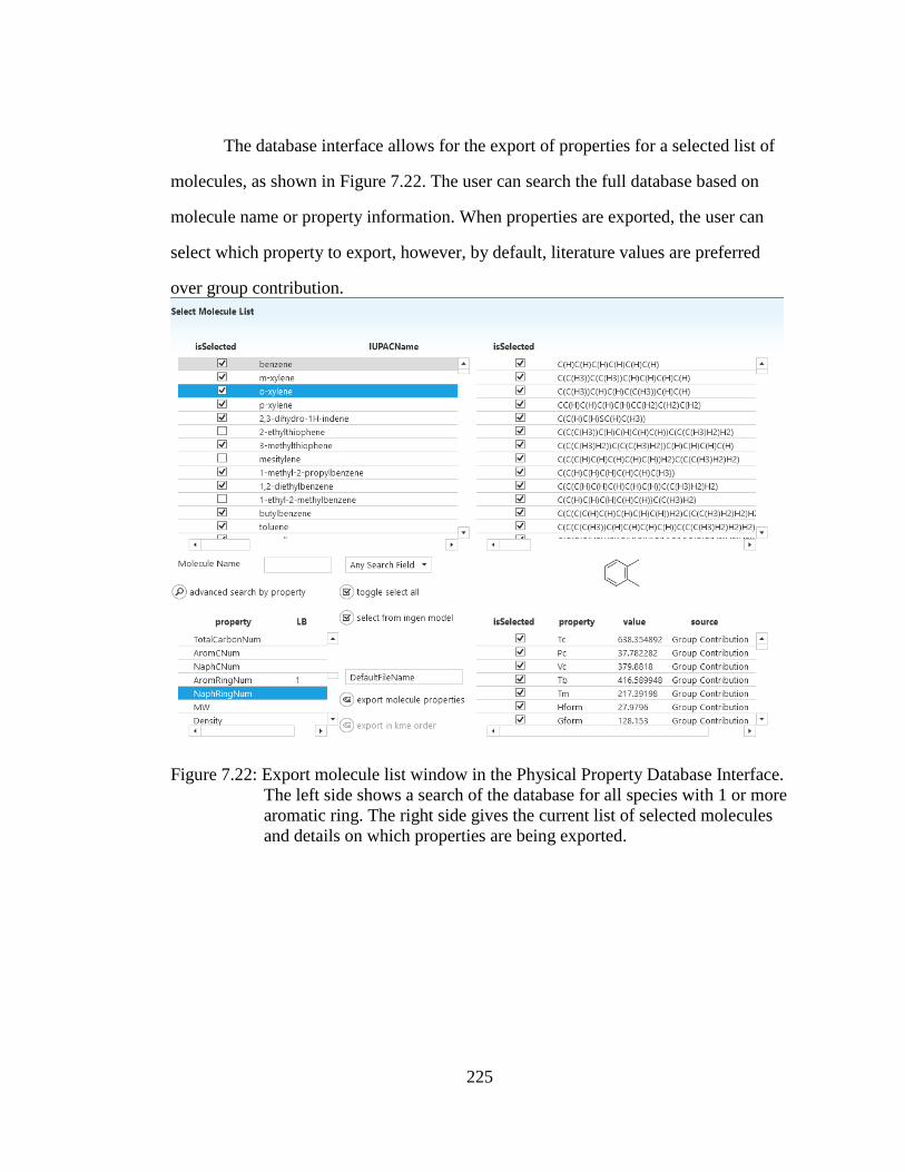
225

The database interface allows for the export of properties for a selected list of

molecules, as shown in Figure 7.22. The user can search the full database based on

molecule name or property information. When properties are exported, the user can

select which property to export, however, by default, literature values are preferred

over group contribution.

Figure 7.22: Export molecule list window in the Physical Property Database Interface.

The left side shows a search of the database for all species with 1 or more

aromatic ring. The right side gives the current list of selected molecules

and details on which properties are being exported.

226

7.4 Current and Future App Development

A key benefit to the app-based style of software design is that development is

quick and ongoing. Unlike with major software packages, the timeframe between idea

conception and availability of a usable tool is much shorter. This section details the

Data Audit Application, a project currently still in the conception stage. A second

advantage of app development is the ease of version updates. Currently, many of the

apps are going through a general UI update. Over the last two years of developing

apps, the quality of the user interfaces has improved drastically.

7.4.1 Data Audit Application

In the future, the idea of a ‘data audit’ will be explored. As a modeler, the

default is to trust experimental data and, instead, question the correctness of the model

if model and experiment do not agree. The typical course of action is to then go back

to tuning the kinetic model or explore the reaction network to understand if any

process chemistry is missing from the model. The idea of the data audit is to perform a

heuristic to analyze the experimental data. There are two tiers currently being

considered: analyzing the data alone, and analyzing the data and reaction network

simultaneously.

The first tier heuristic is to analyze the consistency of experimental data with

itself. Basic examples of this are mass balances: i.e., do the measured weight fractions

sum to 1.0? This type of analysis catches many types of human errors such as

erroneous entry of data. Comparing experimental data on the input and output can

provide more useful information. This is most useful if there are molecular

measurements on both streams. In this case, a carbon balance can be calculated using

227

Equation 7.5. If the carbon balance is nonzero, then no amount of tuning of model

parameters will return perfect results.

𝐶𝑎𝑟𝑏𝑜𝑛 𝐵𝑎𝑙𝑎𝑛𝑐𝑒

= ∑ (𝐶#,𝑖 ∗ 𝑚𝑜𝑙𝑎𝑟𝐹𝑙𝑜𝑤𝑖)

𝑛𝑢𝑚𝐼𝑛𝑝𝑢𝑡𝑠

𝑖=0

− ∑ (𝐶#,𝑗 ∗ 𝑚𝑜𝑙𝑎𝑟𝐹𝑙𝑜𝑤𝑗)

𝑛𝑢𝑚𝑂𝑏𝑠

𝑗=0

(7.5)

Figure 7.23: Basic reaction network layout for heuristic example.

Table 7.11: Inputs, observed quantities, minimum and possible values at reactor outlet,

and whether a heuristic returns a red flag.

Species Input

(Mol/s)

Observed

(Mol/s)

Min,

Max

Red Flag from

Heuristic

A 1 0 0, 1 N

F 2 0 0, 2 N

B 0 2 0, 3 N

E 0 2 0, 1 Y

A second tier heuristic is to analyze both the data and reaction network. The

major question asked by this heuristic is: can the data be predicted given the structure

of the reaction network? A simple, conceptual example is shown below in Figure 7.8

228

and Table 7.11. Based on the input of A and F into the network, the maximum

production of B is 3 Mol/s if all of both A and F react to B. In this example, the

observed amount of B is 2 Mol/s, which is less than the maximum, and the heuristic

does not flag the measurement. For E, the observed value is 2 Mol/s and the maximum

possible production is 1 Mol/s based on the structure of the reaction network. The

heuristic returns a flag, which means that either the data or the reaction network needs

to be edited. No amount of kinetic parameter tuning will ever produce the observed

value of E.

7.4.2 Update of User Interfaces

Currently, many of the older apps are going through an update of their user

interfaces. Specifically, app development has switched from Windows Forms

Applications to the more modern Windows Presentation Foundation (WPF). From the

point of view of app development, the main advantage of WPF is ability of elements

(e.g., menus) to be easily replicated across applications. The built-in objects in WPF

are also much more visually appealing.

229

Figure 7.24: Comparison of user interfaces in Windows Forms Applications (Left,

App: INGen Network Merge) and Windows Presentation Foundation

(WPF, Physical Properties Database Interface).

7.5 Summary

In summary, software development in KMT has shifted toward lightweight

software apps. These apps target the objectives of the kinetic model’s users. The first

category of apps aimed at elucidating the detailed results from kinetic models to help

improve model comprehension. These apps included the visualization of reaction

networks and the visualization of reactor profile data. The second category of apps

focused on measured inputs and outputs to the process. These apps are tailored to

individual processes and collaborators. Most importantly, by focusing on inputs and

outputs, the learning curve to using KMT is minimized. The final group of apps

focuses on enhancing the capabilities of KMT. These apps are wide-ranging and

include flowsheeting, simulating TGA, and an interface to a physical properties

database. As a developer, the apps of KMT are inherently rewarding as they target the

needs of specific users. All apps are currently in use by either researchers or industrial

collaborators.

230

SUMMARY AND CONCLUSIONS

8.1 Summary and Conclusions

In summary, this dissertation presented two orthogonal goals: the development

of kinetic models and the development of model building tools. A model for the

gasification of MSW was generated and solved using the in-house KMT software.

This was accomplished in three phases. In the first two phases, gasification models for

biomass and plastics were developed, independently, and optimized using literature

data. These models were merged to form a gasification reaction model for MSW. This

model, combined with a coke gasification reaction model, provided the basis for a

reactor model of a plasma-arc gasifier. The reactor model represented the gasifier

using four beds, corresponding to different zones in the overall gasification unit.

The plasma-arc gasifier reactor model was utilized for trending studies and

helped to understand the effects of the extreme temperatures in the combustion zone of

the reactor, the impact of MSW composition, and the effects of changing the oxygen

flow rates, or the equivalence ratio. The extreme temperatures of the combustion zone

were found to potentially increase tar production and reduce syngas quality due to a

localized conversion of CO to CO2. Realistic variations of MSW composition was

found to have a minor impact on syngas quality, provided that equivalence ratio

remained constant. The effects on tar composition were more pronounced, with higher

Chapter 8

231

biomass fractions leading to increased production of oxygenated aromatics, and higher

plastics fractions leading to increased production of benzene and naphthalene. Finally,

increasing oxygen flow rate to the bed decreased both tar flow rate and syngas quality.

This provides room for optimization by process engineers to maximize syngas quality

while keeping tar formation within the design specifications for downstream

operations.

In the process of modeling MSW gasification, modeling strategies were

developed for both linear and cross-linked polymers. These strategies extend to other

feedstocks such as additional plastics and entirely different complex feedstocks. For

instance, the same modeling strategies utilized for lignin were applied to the pyrolysis

of heavy oil. Going forward, the study of additional plastics and other, more complex

feedstocks such as coal will be expedited due to the development of modeling

strategies in this dissertation.

While building the models for MSW gasification and resid pyrolysis, software

‘apps’ were developed to aid in future model development. A key aim of software

development was to target the user-model interface. Specifically, there are three

groups of users: model developers, research collaborators, and process engineers; each

group has their own goals while using the model. Process engineers are most

interested in the ability of the model to predict measurable outputs from measurable

inputs. The perfect tool for a process engineer is just that: an I/O converter. In addition

to the measurable I/O, research collaborators care about the scientific and

mathematical understanding of the model. These users wish to understand the process

chemistry to improve results in the long run. Model developers share these aims with

the research collaborators; however, they are also interested in the future development

232

of models. Apps that are exclusive to model developers add features to KMT to aid in

future projects.

8.2 Recommendations for Future Work

8.2.1 MSW Composition

The composition of MSW is one major area for future research in both the

composition of individual polymers and the overall composition of waste. For the

composition of linear polymers, there are two potential areas of future work. First, the

assumptions of this model led to deviations between measured and modeled ultimate

analyses for some polymers. Second, real MSW contains more than a single sample of

each polymer. For the overall composition of waste, the suggested focus area for

research is a method of quantification of polymer fractions in daily gasifier operation.

8.2.1.1 Individual Polymer Composition

In the modeling of the composition of linear polymers, the data utilized were

from ultimate analyses. To utilize this limited data, two constraints were imposed in

the composition model. First, the linear polymers were assumed to have known and

constant repeat unit structure. Second, the polymer size distribution was assumed to

follow an idealized distribution, e.g., a Flory distribution[61]. Although these

assumptions worked well for some polymers, others—such as PVC—showed

deviations when compared with experimental ultimate analysis. A preliminary

analysis of these deviations is given in the following text; however, this is suggested

as an area for future consideration.

The comparison of the PVC composition model with literature experimental

results is given in Table 8.1. The deviations are seen in the relative amounts of carbon

233

and chlorine in the polymer sample. For PVC, a Flory distribution was assumed to

model the polymer size distribution. If this assumption is relaxed, one can imagine two

extremes: all monomers or an infinite polymer. In either of these scenarios, the amount

of carbon is still below that of the experimental value. Therefore, polymer size

distribution alone cannot explain this discrepancy.

The second possible reason for deviation between experiments and model

predictions is the assumption of a constant repeat unit in the polymer sample. This

assumption is a bit more interesting. First, real PVC waste can contain many

plasticizers. However, these plasticizers typically originate from phthalates, which

contain oxygen. The absence of oxygen from the ultimate analysis excludes

plasticizers from consideration. However, it is also known that the first step of

depolymerization is fast in PVC, forming a polyene structure with C2H2 repeat unit. If

the polymer backbone is assumed to be a mixture of polyene and PVC repeat units,

then the predicted and experimental analyses are significantly closer.

Table 8.1: Experimental[64] and predicted ultimate analyses for PVC. Also given are

the ultimate analyses if the for a monomer and infinite polymer, and pure

polyene structure. The partially depolymerized polymer was 93.6% PVC

repeat units with 6.4% polyene repeat units.

Element Polyvinyl Chloride

Experimental Predicted Monomer Infinite Polymer

Polyene Partial Depoly.

C 41.55 38.1 37.2 38.4 92.3 41.55 H 4.81 5.44 7.8 4.81 7.6 5.57 O 0.00 0.00 0.00 0.00 0.00 0.00 Cl 52.95 56.38 55.0 56.8 0.00 52.78

The only significant change to model results is the amount of HCl produced by

depolymerization. In the original model, depolymerization would convert

234

approximately 56 weight percent of the polymer to HCl; in contrast, the updated

composition would only convert 53 weight percent to HCl. The partial

depolymerization hypothesis did correct the modeled composition to match

experimental results; however future work is needed to verify the results.

Real MSW is inherently complex with multiple sources of each polymer. For

instance, there are many types of polyethylenes, including high-density polyethylene

and low-density polyethylene. In the model presented in this dissertation, each

polymer fraction was optimized using a single ultimate analysis. An area for future

work in MSW composition is in relaxing these assumptions.

One possible route forward is an extensive analysis of common polymer types,

polymer size distributions, and the effects on the output from a kinetic model. In order

to pursue this method, detailed input and output data are required for each polymer in

question. For the inlet, polymer size distributions can be obtained from Gel

Permeation Chromatography[66]. This information can be paired with detailed gas

chromatography results to study the effect of polymer type (e.g., HDPE) for each

polymer on the reaction kinetics. Ultimately, this methodology would allow the model

to take into account a combination of polymers and polymer types. To utilize this level

of detail in a gasifier, additional work is required in modeling the combined

composition of MSW.

8.2.1.2 Combined Composition of MSW

Currently, the composition of the polymeric fractions of MSW is based on an

ultimate analysis, potentially taken daily, during gasifier operation. In this model,

MSW is represented using four plastics and three biopolymers, and an ultimate

analysis likely contains only four usable data points (C, H, O, and Cl). Optimization is

235

therefore under-constrained, and there are infinite solutions for any ultimate analysis.

In current simulations, known samples of MSW (such as the US average distribution)

are utilized; however, in gasifier operation, these values—while representative—will

not be exactly correct.

A potential route for future research lies in relaxing the assumption that the

only available data are from ultimate analyses. This could be done at the plant

operation level, i.e., a method of efficiently quantifying polymeric fractions of waste.

A second option would be to perform a study of the average MSW composition over

time for a given MSW gasifier. This would inform the quantification of individual

MSW fractions beyond that of an ultimate analysis.

8.2.2 Parameter Tuning and Confidence Intervals

In this dissertation, the final set of parameters for the MSW gasification model

was based on literature studies on plastics and biomass. In the future, with the

availability of plant data, we hope to access the validity of our current parameter

values in a commercial scale gasifier. If intrinsic values of kinetic parameters were

obtained in literature studies, then the model results should match the full gasifier.

Issues could arise as the temperatures of the plasma gasifier are much more extreme

than the literature studies utilized for parameter tuning. Also, the plant is at a large

scale of 1,000 metric tons/day. If there are mass or heat transfer limitations, there is

opportunity for future model development and parameter tuning.

The parameters in a kinetic model can be assessed using statistics. For

example, using the seven data sets in the biomass gasification study, confidence

intervals can be calculated for the tuned parameters. Specifically, we have predicted

95% confidence intervals using methodology described in prior work by Hou[43]. The

236

relative confidence intervals on the pre-exponential, or A, factors are given in Figure

8.1. The confidence intervals were smallest on depolymerization and gasification

chemistries. The A-factors were less certain on cracking and dehydrogenation; at the

reactor conditions, these reaction families are relatively fast and small changes do not

appear in the objective function. In contrast, the objective function was insensitive to

the dry reforming of methane because the reaction rate is too slow. In this case, minor

increases in the A-factor do not increase the rate enough to impact the objective

function. In the future, with the availability of data for MSW gasification we can

extend this methodology to the reactor model of the plasma-arc gasifier.

Figure 8.1: 95% confidence intervals on A-factors relative to the value of the A-factor.

For instance, the confidence interval is ±0.169 ∗ 𝑙𝑜𝑔𝐴 for

dehydrogenation.

0.00

0.02

0.04

0.06

0.08

0.10

0.12

0.14

0.16

0.18

Rel

ativ

e 9

5%

Co

nfi

den

ce In

terv

al o

n A

-fac

tors

237

8.2.3 Optimizing Experimental Data for Molecular Models

The current limits to molecular-level modeling of MSW gasification are

imposed, not by the modeling methods or computational power, but by the

experimental information available in gasification literature. In order to enable the use

of molecular models, future gasification literature should focus on molecular detail of

both the reactor inlet and reactor outlet. For the reactor inlet, currently ultimate

analyses are the most common characterization. For the reactor outlet, the common

results are tar weight fraction and molecular predictions from gas chromatography on

the most common species(CO, CO2, H2, and CH4). On both the inlet and outlet, this

status quo lacks molecular detail. This is not necessarily due to a lack of experimental

techniques; a full spectrum of advanced experiments is seen in the literature on

refinery reactors. These experiments have aided in the development of detailed kinetic

models on a wide range of boiling point ranges from naphtha[135]–[140] to vacuum

gas oil[141] to vacuum resid[46], [48], [127]–[130].

In naphtha reforming, molecular models are enabled through extensive

molecular detail on both the input and output. For instance, standard measurements

include simulated distillation, density, and carbon number PIONA. Advanced

measurements such as GCxGC can give many isomers of species with up to 14

carbons[142], [143]. These measurements enable molecular models by allowing for

mechanism discrimination and accurate kinetic parameter tuning.

The most complex refinery units also utilize advanced experiments to enable

molecular modeling. For example, in heavy oil coker, FTICR-MS (Fourier Transform

Ion Cyclotron Resonance-Mass Spectrometry) is utilized to elucidate the molecular

identities of up to 50,000 unique species[46],[124]. These measurements can be

utilized in molecular models as shown in Figure 8.2[46]. The degree of complexity in

238

heavy oil is on the same order of magnitude as MSW. This gives cause for optimism

for the future pairing of detailed experiments and detailed kinetic models.

Figure 8.2: Comparison of DBE versus Carbon Number for single pyrollic ring

structures for experimental(right) and predicted (left) results. Figure

taken directly from source and was Figure 15 in the source material.[46]

8.3 Closing Remarks on MSW Gasification

Currently, much of the waste in the United States is discarded in landfills.

MSW is a valuable energy resource that is one of the low-hanging fruits in the energy

market, and is able to provide a significant amount of cheap energy with little research

and development. In order to pursue this source of energy, there are a number of

useful Waste-to-Energy (WTE) technologies. This dissertation focused on

gasification of waste, and culminated in a reactor model for the most environmentally

friendly WTE option: plasma-arc gasification. In building this model, it was shown

that the process could be modeled at the molecular-level. This model is based on

fundamental process chemistry and can account for changes in process conditions and

MSW composition. Gasification and other WTE technologies have been, and will

continue to be, a future topic of research. Undoubtedly, detailed kinetic models will

play a central role in the future conversion of waste to energy.

239

[1] EPA, “Advancing Sustainable Materials Management: Facts and Figures 2013,”

2015.

[2] B. W. Mosher, P. M. Czepiel, R. C. Harriss, J. H. Shorter, C. E. Kolb, J. B.

McManus, E. Allwine, and B. K. Lamb, “Methane Emissions at Nine Landfill

Sites in the Northeastern United States,” Environ. Sci. Technol., vol. 33, no. 12,

pp. 2088–2094, Jun. 1999.

[3] EPA, “LFG Energy Project Development Handbook,” 2015.

[4] E. Braw, “Dirty power: Sweden wants your garbage for energy,” Aljazeera

America, 2015.

[5] Department for Environmental and Rural Affairs, “Incineration of Municipal

Solid Waste,” 2013.

[6] G. C. Young, Municipal Solid Waste to Energy Conversion Processes

Economic, Technical, and Renewable Comparisons. Hobeken, NJ: John Wiley

& Sons, Inc., 2010.

[7] H. . Chagger, A. Kendall, A. McDonald, M. Pourkashanian, and A. Williams,

“Formation of dioxins and other semi-volatile organic compounds in biomass

combustion,” Appl. Energy, vol. 60, no. 2, pp. 101–114, 1998.

[8] EPA, Clean Air Act. 42 U.S.C. §7401, 1990.

[9] D. A. Bell, B. F. Towler, and M. Fan, Coal Gasification and Its Applications.

William Andrew Applied Science Publishers, 2011.

[10] A. Grupping, “Coal Gasification Method,” 4,243,101, 1981.

[11] J. L. Johnson, Kinetics of Coal Gasification A Compliation of the Research by

the late Dr. James Lee Johnson. John Wiley & Sons, Inc., 1979.

[12] J. Rezaiyan and N. P. Cheremisinoff, Gasification Technologies a primer for

engineers and scientists. Taylor & Francis Group, 2005.

REFERENCES

240

[13] X. T. Li, J. R. Grace, C. J. Lim, a. P. Watkinson, H. P. Chen, and J. R. Kim,

“Biomass gasification in a circulating fluidized bed,” Biomass and Bioenergy,

vol. 26, no. 2, pp. 171–193, Feb. 2004.

[14] H. J. Huang and S. Ramaswamy, “Modeling biomass gasification using

thermodynamic equilibrium approach,” Appl. Biochem. Biotechnol., vol. 154,

no. 1–3, pp. 193–204, 2009.

[15] Y. Wang and C. M. Kinoshita, “Kinetic model of biomass gasification,” Sol.

Energy, vol. 51, no. 1, pp. 19–25, 1993.

[16] M. Puig-Arnavat, J. C. Bruno, and A. Coronas, “Review and analysis of

biomass gasification models,” Renew. Sustain. Energy Rev., vol. 14, no. 9, pp.

2841–2851, Dec. 2010.

[17] M. Ruggiero and G. Manfrida, “An equilibrium model for biomass gasification

processes,” Renew. Energy, vol. 16, no. 1–4, pp. 1106–1109, 1999.

[18] D. C. Elliott, “Catalyic Hydrothermal Gasification of Biomass,” Biofuels,

Bioprod. Biorefining, vol. 2, pp. 254–265, 2008.

[19] P. R. Solomon, D. G. Hamblen, R. M. Carangelo, M. A. Serio, and G. V

Deshpande, “General Model of Coal Devolatilizationt,” vol. 24, no. 3, pp. 405–

422, 1988.

[20] H. Wang, B. Z. Dlugogorski, and E. M. Kennedy, “Coal oxidation at low

temperatures: oxygen consumption, oxidation products, reaction mechanism

and kinetic modelling,” Prog. Energy Combust. Sci., vol. 29, no. 6, pp. 487–

513, Jan. 2003.

[21] U. Arena, “Process and technological aspects of municipal solid waste

gasification. A review,” Waste Manag., vol. 32, no. 4, pp. 625–639, 2012.

[22] E. Leal-Quirós, “Plasma Processing of Municipal Solid Waste,” Brazilian J.

Phys., vol. 34, no. 4B, pp. 1587–1593, 2004.

[23] U. Arena, L. Zaccariello, and M. L. Mastellone, “Tar removal during the

fluidized bed gasification of plastic waste.,” Waste Manag., vol. 29, no. 2, pp.

783–91, Feb. 2009.

[24] B. Lemmens, H. Elslander, I. Vanderreydt, K. Peys, L. Diels, M. Oosterlinck,

and M. Joos, “Assessment of plasma gasification of high caloric waste

streams,” Waste Manag., vol. 27, no. 11, pp. 1562–1569, 2007.

241

[25] A. J. Griffiths, K. P. Williams, and N. Owen, “Engineering value recovery from

municipal solid waste,” Proc. Inst. Mech. Eng. Part C J. Mech. Eng. Sci., vol.

224, no. 3, pp. 559–570, 2010.

[26] S. Jarungthammachote and A. Dutta, “Equilibrium modeling of gasification:

Gibbs free energy minimization approach and its application to spouted bed and

spout-fluid bed gasifiers,” Energy Convers. Manag., vol. 49, no. 6, pp. 1345–

1356, 2008.

[27] S. Jarungthammachote and A. Dutta, “Thermodynamic equilibrium model and

second law analysis of a downdraft waste gasifier,” Energy, vol. 32, no. 9, pp.

1660–1669, 2007.

[28] A. K. Sharma, “Equilibrium modeling of global reduction reactions for a

downdraft (biomass) gasifier,” Energy Convers. Manag., vol. 49, no. 4, pp.

832–842, 2008.

[29] H. Tang and K. Kitagawa, “Supercritical water gasification of biomass:

Thermodynamic analysis with direct Gibbs free energy minimization,” Chem.

Eng. J., vol. 106, no. 3, pp. 261–267, 2005.

[30] Z. A. Zainal, R. Ali, C. H. Lean, and K. N. Seetharamu, “Prediction of

performance of a downdraft gasifier using equilibrium modeling for different

biomass materials,” Energy Convers. Manag., vol. 42, no. 12, pp. 1499–1515,

2001.

[31] I. Janajreh, S. S. Raza, and A. S. Valmundsson, “Plasma gasification process:

Modeling, simulation and comparison with conventional air gasification,”

Energy Convers. Manag., vol. 65, pp. 801–809, 2013.

[32] X. Li, J. R. Grace, A. P. Watkinson, C. J. Lim, and A. Ergudenler, “Equilibrium

modeling of gasification: A free energy minimization approach and its

application to a circulating fluidized bed coal gasifier,” Fuel, vol. 80, no. 2, pp.

195–207, 2001.

[33] A. Mountouris, E. Voutsas, and D. Tassios, “Solid waste plasma gasification:

Equilibrium model development and exergy analysis,” Energy Convers.

Manag., vol. 47, no. 13–14, pp. 1723–1737, 2006.

[34] Q. Zhang, L. Dor, A. K. Biswas, W. Yang, and W. Blasiak, “Modeling of steam

plasma gasification for municipal solid waste,” Fuel Process. Technol., vol.

106, pp. 546–554, 2013.

[35] Q. Zhang, L. Dor, W. Yang, and W. Blasiak, “Eulerian model for municipal

242

solid waste gasification in a fixed-bed plasma gasification melting reactor,”

Energy and Fuels, vol. 25, no. 9, pp. 4129–4137, 2011.

[36] J. M. Zurada, Introduction to artificial neural systems, vol. 8. West publishing

company St. Paul, 1992.

[37] G. Xiao, M. jiang Ni, Y. Chi, B. Jin, R. Xiao, Z. Zhong, and Y. Huang,

“Gasification characteristics of MSW and an ANN prediction model,” Waste

Manag., vol. 29, no. 1, pp. 240–244, 2009.

[38] L. Broadbelt, S. Stark, and M. Klein, “Computer generated reaction modelling:

decomposition and encoding algorithms for determining species uniqueness,”

Comput. Chem. Eng., vol. 20, no. 2, pp. 113–129, 1996.

[39] L. J. Broadbelt, S. M. Stark, and M. T. Klein, “Computer Generated Pyrolysis

Modeling: On-the-Fly Generation of Species, Reactions, and Rates,” Ind. Eng.

Chem. Res., vol. 33, no. 4, pp. 790–799, Apr. 1994.

[40] W. Wei, C. A. Bennett, R. Tanaka, G. Hou, M. T. J. Klein, and M. T. Klein,

“Computer aided kinetic modeling with KMT and KME,” Fuell Process.

Technol., vol. 89, p. 350, 2008.

[41] M. T. Klein, G. Hou, R. J. Quann, W. Wei, K. H. Liao, R. S. H. Yang, J. a

Campain, M. a Mazurek, and L. J. Broadbelt, “BioMOL: a computer-assisted

biological modeling tool for complex chemical mixtures and biological

processes at the molecular level.,” Environ. Health Perspect., vol. 110 Suppl ,

pp. 1025–9, Dec. 2002.

[42] M. T. Klein, G. Hou, R. J. Bertolacini, L. J. Broadbelt, and A. Kumar,

Molecular Modeling in Heavy Hydrocarbon Conversions. Boca Raton, FL:

Taylor and Francis Group, 2006.

[43] Z. Hou, “Software Tools for Molecule-based Kinetic Modeling of Complex

Systems,” Rutgers University, 2011.

[44] C. A. Bennett, “User-Controlled Kinetic Network Generation with INGen,”

Rutgers University, 2009.

[45] B. M. Moreno, “Thermochemical Conversion of Biomass: Models and

Modelling Approaches,” University of Delaware, 2014.

[46] L. Zhang, Z. Hou, S. R. Horton, M. T. Klein, Q. Shi, S. Zhao, and C. Xu,

“Molecular Representation of Petroleum Vacuum Resid,” Energy & Fuels, vol.

28, pp. 1736–1749, Mar. 2014.

243

[47] S. Horton and M. Klein, “Reaction and Catalyst Families in the Modeling of

Coal and Biomass Hydroprocessing Kinetics,” Energy & Fuels, vol. 28, no.

2013, pp. 37–40, 2013.

[48] S. R. Horton, Z. Hou, B. M. Moreno, C. A. Bennett, and M. T. Klein,

“Molecule-based modeling of heavy oil,” Sci. China Chem., vol. 56, no. 7, pp.

840–847, Jun. 2013.

[49] I. Mochida and Y. Yoneda, “Linear free energy relationships in heterogeneous

catalysis: II. Dealkylation and isomerization reactions on various solid acid

catalysts,” J. Catal., vol. 7, pp. 393–396, 1967.

[50] C. Read, “Reactor and Catalyst Structure/function Relationships in the

Hydrocracking of Alkyl-substituted Biphenyl Compounds,” University of

Delaware, 1995.

[51] M. Evans and M. Polanyi, “Some applications of the transition state method to

the calculation of reaction velocities, especially in solution,” Trans. Faraday

Soc., 1935.

[52] R. Bell, “The theory of reactions involving proton transfers,” Proc. R. Soc.

London. Ser. A, 1936.

[53] K. Radhakrishnan and A. Hindmarsh, “Description and use of LSODE, the

Livermore solver for ordinary differential equations,” NASA, 1993.

[54] S. R. Horton, J. Woeckener, R. J. Mohr, Y. Zhang, F. P. Petrocelli, and M. T.

Klein, “Molecular-Level Kinetic Modeling of the Gasification of Common

Plastics,” Energy Fuels (In Press., 2015.

[55] T. M. Kruse, O. S. Woo, H.-W. Wong, S. S. Khan, and L. J. Broadbelt,

“Mechanistic Modeling of Polymer Degradation: A Comprehensive Study of

Polystyrene,” Macromolecules, vol. 35, no. 20, pp. 7830–7844, Sep. 2002.

[56] T. M. Kruse, O. Sang Woo, and L. J. Broadbelt, “Detailed mechanistic

modeling of polymer degradation: application to polystyrene,” Chem. Eng. Sci.,

vol. 56, no. 3, pp. 971–979, Feb. 2001.

[57] D. M. Matheu and J. M. Grenda, “A systematically generated, pressure-

dependent mechanism for high-conversion ethane pyrolysis. 1. Pathways to the

minor products,” J. Phys. Chem. A, vol. 109, no. 24, pp. 5332–5342, 2005.

[58] T. Faravelli, G. Bozzano, M. Colombo, E. Ranzi, and M. Dente, “Kinetic

modeling of the thermal degradation of polyethylene and polystyrene

244

mixtures,” J. Anal. Appl. Pyrolysis, vol. 70, no. 2, pp. 761–777, 2003.

[59] E. Henrich, S. Bürkle, Z. I. Meza-Renken, and S. Rumpel, “Combustion and

gasification kinetics of pyrolysis chars from waste and biomass,” J. Anal. Appl.

Pyrolysis, vol. 49, no. 1, pp. 221–241, 1999.

[60] X. H. Du, C. S. Zhao, Y. Z. Wang, Q. Zhou, Y. Deng, M. H. Qu, and B. Yang,

“Thermal oxidative degradation behaviours of flame-retardant thermotropic

liquid crystal copolyester/PET blends,” Mater. Chem. Phys., vol. 98, no. 1, pp.

172–177, 2006.

[61] P. J. Flory, Principles of Polymer Chemistry. New York: Cornell, 1953.

[62] Kirk-Othmer, Kirk-Othmer Encyclopedia of Chemical Technology, vol. 24.

1997.

[63] J. M. Heikkinen, J. C. Hordijk, W. De Jong, and H. Spliethoff,

“Thermogravimetry as a tool to classify waste components to be used for

energy generation,” J. Anal. Appl. Pyrolysis, vol. 71, no. 2, pp. 883–900, 2004.

[64] H. M. Zhu, X. G. Jiang, J. H. Yan, Y. Chi, and K. F. Cen, “TG-FTIR analysis

of PVC thermal degradation and HCl removal,” J. Anal. Appl. Pyrolysis, vol.

82, no. 1, pp. 1–9, 2008.

[65] C. Bouster, P. Vermande, and J. Veron, “Evolution of the product yield with

temperature and molecular weight in the pyrolysis of polystyrene,” J. Anal.

Appl. Pyrolysis, vol. 15, pp. 249–259, 1989.

[66] C. M. Stafford, T. P. Russell, and T. J. McCarthy, “Expansion of polystyrene

using supercritical carbon dioxide: effects of molecular weight, polydispersity,

and low molecular weight components,” Macromolecules, vol. 32, no. 22, pp.

7610–7616, 1999.

[67] Y. Liu, J. Qian, and J. Wang, “Pyrolysis of polystyrene waste in a fluidized-bed

reactor to obtain styrene monomer and gasoline fraction,” Fuel Process.

Technol., vol. 63, no. 1, pp. 45–55, 2000.

[68] N. Grassie and G. Scott, Polymer Degradation and Stabilisation. Great Britain:

Press Syndicate of the University of Cambrdige, 1985.

[69] J. D. Peterson, S. Vyazovkin, and C. A. Wight, “Kinetics of the Thermal and

Thermo-Oxidative Degradation of Polystyrene, Polyethylene and

Poly(propylene),” Macromol. Chem. Phys., vol. 202, no. 6, p. 775, 2001.

245

[70] G. Montaudo, C. Puglisi, and F. Samperi, “Primary thermal degradation

mechanisms of PET and PBT,” Polymer Degradation and Stability, vol. 42, no.

1. pp. 13–28, 1993.

[71] L. H. Buxbaum, “The Degradation of Poly(ethylene terephthalate),” Angew.

Chemie Int. Ed., vol. 7, no. 3, p. 182, 1968.

[72] B. B. Troitskii, L. S. Troitskaya, V. N. Myakov, and A. F. Lepaev, “Mechanism

of the thermal degradation of poly(vinyl chloride),” J. Polym. Sci., vol. 1361,

no. 42, pp. 1347–1361, 1973.

[73] Y. Tsuchiya and K. Sumi, “Thermal decomposition products of poly(vinyl

alcohol),” J. Polym. Sci. Part A-1 Polym. Chem., 1969.

[74] B. M. Moreno, N. Li, J. Lee, G. W. Huber, and M. T. Klein, “Modeling

aqueous-phase hydrodeoxygenation of sorbitol over Pt/SiO2–Al2O3,” RSC

Adv., vol. 3, no. 45, p. 23769, 2013.

[75] J. Zhang, Q. Ji, P. Zhang, Y. Xia, and Q. Kong, “Thermal stability and flame-

retardancy mechanism of poly(ethylene terephthalate)/boehmite

nanocomposites,” Polym. Degrad. Stab., vol. 95, no. 7, pp. 1211–1218, 2010.

[76] X. H. Du, Y. Z. Wang, X. T. Chen, and X. D. Tang, “Properties of phosphorus-

containing thermotropic liquid crystal copolyester/poly(ethylene terephthalate)

blends,” Polym. Degrad. Stab., vol. 88, no. 1, pp. 52–56, 2005.

[77] J. Zhang, Q. Ji, P. Zhang, Y. Xia, and Q. Kong, “Thermal stability and flame-

retardancy mechanism of poly(ethylene terephthalate)/boehmite

nanocomposites,” Polym. Degrad. Stab., vol. 95, no. 7, pp. 1211–1218, 2010.

[78] V. Cozzani, C. Nicolella, M. Rovatti, and L. Tognotti, “Influence of Gas-Phase

Reactions on the Product Yields Obtained in the Pyrolysis of Polyethylene,”

Ind. Eng. Chem. Res., vol. 36, no. 2, pp. 342–348, 1997.

[79] V. Cozzani, “Characterization of coke formed in the pyrolysis of polyethylene,”

Ind. Eng. Chem. Res., vol. 36, pp. 5090–5095, 1997.

[80] C. A. Bennett and M. T. Klein, “Using Mechanistically Informed Pathways to

Control the Automated Growth of Reaction Networks,” Energy & Fuels, vol.

26, no. 1, pp. 41–51, Jan. 2012.

[81] F. Bustamante, R. M. Enick, R. P. Killmeyer, B. H. Howard, K. S.

Rothenberger, a. V. Cugini, B. D. Morreale, and M. V. Ciocco, “Uncatalyzed

and wall-catalyzed forward water-gas shift reaction kinetics,” AIChE J., vol. 51,

246

no. 5, pp. 1440–1454, May 2005.

[82] M. J. P. Slapak, J. M. N. Van Kasteren, and B. a a H. Drinkenburg,

“Hydrothermal Recycling of PVC in a Bubbling Fluidized Bed Reactor : the In

¯ uence of Bed Material and Temperature,” Polym. Adv. Technol., vol. 602, pp.

596–602, 1999.

[83] S. R. Horton, R. J. Mohr, Y. Zhang, F. P. Petrocelli, and M. T. Klein,

“Molecular-Level Kinetic Modeling of Biomass Gasification,” Energy & Fuels,

p. acs.energyfuels.5b01988, 2015.

[84] T. L. Richard, “Challenges in scaling up biofuels infrastructure.,” Science, vol.

329, pp. 793–796, 2010.

[85] H. . Chagger, a Kendall, a McDonald, M. Pourkashanian, and a Williams,

“Formation of dioxins and other semi-volatile organic compounds in biomass

combustion,” Appl. Energy, vol. 60, no. 2, pp. 101–114, 1998.

[86] D. K. Shen, S. Gu, K. H. Luo, a. V. Bridgwater, and M. X. Fang, “Kinetic

study on thermal decomposition of woods in oxidative environment,” Fuel, vol.

88, no. 6, pp. 1024–1030, Jun. 2009.

[87] M. Broström, a. Nordin, L. Pommer, C. Branca, and C. Di Blasi, “Influence of

torrefaction on the devolatilization and oxidation kinetics of wood,” J. Anal.

Appl. Pyrolysis, vol. 96, pp. 100–109, Jul. 2012.

[88] L. Zhong and W. Mei, “Kinetic Model Establishment and Verficiation of the

Biomass Gasificaiton on Fluidized Bed,” no. July, pp. 12–15, 2009.

[89] N. Prakash and T. Karunanithi, “Kinetic Modeling in Biomass Pyrolysis – A

Review,” vol. 4, no. 12, pp. 1627–1636, 2008.

[90] D. M. Grant, R. J. Pugmire, T. H. Fletcher, and A. R. Kerstein, “Chemical

model of coal devolatilization using percolation lattice statistics,” Energy &

Fuels, vol. 3, no. 2, pp. 175–186, Mar. 1989.

[91] T. H. Fletcher, A. R. Kerstein, R. J. Pugmire, M. S. Solum, and D. M. Grant,

“Chemical Percolation Model for Devolatilization . 3 . Direct Use of 13C NMR

Data To Predict Effects of Coal Type,” no. 10, pp. 414–431, 1992.

[92] T. H. Fletcher, A. R. Kerstein, R. J. Pugmire, and D. M. Grant, “Chemical

Percolation Model for Devolatilization. 2. Temperature and Heating Rate

Effects on Product YieMst,” no. 1, pp. 54–60, 1990.

247

[93] T. H. Fletcher, H. R. Pond, J. Webster, J. Wooters, and L. L. Baxter,

“Prediction of tar and light gas during pyrolysis of black liquor and biomass,”

Energy and Fuels, vol. 26, no. 6, pp. 3381–3387, 2012.

[94] A. D. Lewis and T. H. Fletcher, “Prediction of sawdust pyrolysis yields from a

flat-flame burner using the CPD model,” Energy and Fuels, vol. 27, pp. 942–

953, 2013.

[95] C. Sheng and J. L. T. Azevedo, “Modeling biomass devolatilization using the

chemical percolation devolatilization model for the main components,” Proc.

Combust. Inst., vol. 29, no. 1, pp. 407–414, 2002.

[96] D. Fiaschi and M. Michelini, “A two-phase one-dimensional biomass

gasifcation kinetics model,” Biomass and Bioenergy, vol. 21, pp. 121–132,

2001.

[97] R. Pettersen, “The chemical composition of wood,” Chem. solid wood, 1984.

[98] D. K. Shen, S. Gu, and a. V. Bridgwater, “Study on the pyrolytic behaviour of

xylan-based hemicellulose using TG–FTIR and Py–GC–FTIR,” J. Anal. Appl.

Pyrolysis, vol. 87, no. 2, pp. 199–206, Mar. 2010.

[99] A. C. C. Chang, H.-F. Chang, F.-J. Lin, K.-H. Lin, and C.-H. Chen, “Biomass

gasification for hydrogen production,” Int. J. Hydrogen Energy, vol. 36, no. 21,

pp. 14252–14260, Oct. 2011.

[100] C. Couhert, J.-M. Commandré, and S. Salvador, “Failure of the component

additivity rule to predict gas yields of biomass in flash pyrolysis at 950°C,”

Biomass and Bioenergy, vol. 33, no. 2, pp. 316–326, Feb. 2009.

[101] C. Couhert, J.-M. Commandre, and S. Salvador, “Is it possible to predict gas

yields of any biomass after rapid pyrolysis at high temperature from its

composition in cellulose, hemicellulose and lignin?,” Fuel, vol. 88, no. 3, pp.

408–417, Mar. 2009.

[102] K. Freudenberg, “Lignin: Its Constitution and Formation from p-

Hydroxycinnamyl Alcohols: Lignin is duplicated by dehydrogenation of these

alcohols; intermediates explain formation and structure.,” Science, vol. 148, pp.

595–600, 1965.

[103] A. Tejado, C. Peña, J. Labidi, J. M. Echeverria, and I. Mondragon, “Physico-

chemical characterization of lignins from different sources for use in phenol-

formaldehyde resin synthesis.,” Bioresour. Technol., vol. 98, no. 8, pp. 1655–

63, May 2007.

248

[104] R. El Hage, N. Brosse, L. Chrusciel, C. Sanchez, P. Sannigrahi, and A.

Ragauskas, “Characterization of milled wood lignin and ethanol organosolv

lignin from miscanthus,” Polym. Degrad. Stab., vol. 94, no. 10, pp. 1632–1638,

Oct. 2009.

[105] A. Demirbas, “Products from Lignocellulosic Materials via Degradation

Processes,” Energy Sources, Part A Recover. Util. Environ. Eff., vol. 30, no. 1,

pp. 27–37, Nov. 2007.

[106] F. Shafizadeh, R. H. Furneaux, T. G. Cochran, J. P. Scholl, and Y. Sakai,

“Production of levoglucosan and glucose from pyrolysis of cellulosic

materials,” J. Appl. Polym. Sci., vol. 23, no. 12, pp. 3525–3539, Jun. 1979.

[107] P. J. Linstrom and W. G. Mallard, “NIST Chemistry WebBook, NIST Standard

Reference Database Number 69,” 2015. [Online]. Available:

http://webbook.nist.gov.

[108] W. F. DeGroot and G. N. Richards, “Relative rates of carbon gasification in

oxygen, steam and carbon dioxide,” Carbon N. Y., vol. 27, no. 2, pp. 247–252,

1989.

[109] S. R. Horton, L. Zhang, Z. Hou, C. a. Bennett, M. T. Klein, and S. Zhao,

“Molecular-Level Kinetic Modeling of Resid Pyrolysis,” Ind. Eng. Chem. Res.,

vol. 54, no. 16, pp. 4226–4235, 2015.

[110] G. Löffler, V. J. Wargadalam, and F. Winter, “Catalytic effect of biomass ash

on CO, CH4 and HCN oxidation under fluidised bed combustor conditions,”

Fuel, vol. 81, pp. 711–717, 2002.

[111] B. W. Mosher, P. M. Czepiel, and R. Harriss C., “Methane Emissions at Nine

Landfill Sites in the Northeastern United States,” Environ. Sci. Technol., vol.

33, no. 12, p. 2088, 1999.

[112] WRAP, “Comparing the cost of alternative waste treatment options,” 2012.

[113] N. J. Themelis, M. J. Castaldi, J. Bhattti, and L. Arsova, “Energy and Economic

Value of Non-recycled Plastics (NRP) and Municipal Solid Wastes (MSW) that

are Currently Landfilled in the Fifty States.”

[114] P. L. Walker, R. L. Taylor, and J. M. Ranish, “An update on the carbon-oxygen

reaction,” Carbon N. Y., vol. 29, no. 3, pp. 411–421, Jan. 1991.

[115] R. Hurt and J. Calo, “Semi-global intrinsic kinetics for char combustion

modeling,” Combust. Flame, vol. 2180, no. 01, 2001.

249

[116] B. Feng and S. K. Bhatia, “On the validity of thermogravimetric determination

of carbon gasification kinetics,” Chem. Eng. Sci., vol. 57, no. 15, pp. 2907–

2920, 2002.

[117] S. Ergun, “Kinetics of the Reaction of Carbon Dioxide with Carbon,” Phys.

Chem., vol. 60, pp. 480–485, 1940.

[118] K. Hüttinger and O. Fritz, “The carbon-carbon dioxide reaction: an extended

treatment of the active-site concept,” Carbon N. Y., vol. 2, no. 4, 1991.

[119] J. Leppälahti and T. Koljonen, “Nitrogen evolution from coal, peat and wood

during gasification: Literature review,” Fuel Process. Technol., vol. 43, 1995.

[120] J. R. Arthur, “Reactions between Carbon and Oxygen,” Trans. Faraday Soc.,

vol. 47, pp. 164–178, 1951.

[121] “chap8@Cupola_HB.pdf,” in Cupola Handbook, 1997, pp. 8–1 – 8–37.

[122] E. J. Swain, “Sulfur, coke, and crude quality -- Conclusion: US crude slate

continues to get heavier, higher in sulfur,” Oil Gas J., vol. 93, no. 2, p. 37,

1995.

[123] W. I. Beaton and R. J. Bertolacini, “Resid Hydroprocessing at Amoco,”

Catalysis Reviews, vol. 33. pp. 281–317, 1991.

[124] R. P. Rodgers and A. M. McKenna, “Petroleum Analysis,” Anal. Chem., vol.

83, p. 4665, 2011.

[125] M. Neurock, C. Libanati, A. Nigam, and M. Klein, “Monte Carlo simulation of

complex reaction systems: Molecular structure and reactivity in modelling

heavy oils,” Chem. Eng. Sci., vol. 45, no. 8, pp. 2083–2088, 1990.

[126] R. Rueda-Velásquez and M. Gray, “Monte Carlo simulation of asphaltenes and

products from thermal cracking,” Energy & Fuels, vol. 28, pp. 2352–2364,

2014.

[127] L. P. de Oliveira, J. J. Verstraete, and M. Kolb, “Simulating vacuum residue

hydroconversion by means of Monte-Carlo techniques,” Catal. Today, vol.

220–222, pp. 208–220, Mar. 2014.

[128] R. Quann and S. Jaffe, “Structure-oriented lumping: describing the chemistry of

complex hydrocarbon mixtures,” Ind. Eng. Chem. Res., pp. 2483–2497, 1992.

[129] L. Tian, B. Shen, and J. Liu, “A Delayed Coking Model Built Using the

Structure-Oriented Lumping Method,” Energy & Fuels, vol. 26, no. 3, pp.

250

1715–1724, Mar. 2012.

[130] L. Zhang, “Molecular-Level Characterization and Process Modeling for Heavy

Petroleum Fractions,” China University of Petroleum, 2014.

[131] L. Nationai, “Description and Use of LSODE , the Livermore Solver for

Ordinary Differential Equations,” 1993.

[132] E. R. Gansner and S. C. North, “An open graph visualization system and its

applications to software engineering,” Softw. Pract. Exp., vol. 30, no. 11, pp.

1203–1233, 2000.

[133] Z. Gao, I. Amasaki, and M. Nakada, “A thermogravimetric study on thermal

degradation of polyethylene,” J. Anal. Appl. Pyrolysis, vol. 67, no. 1, pp. 1–9,

Mar. 2003.

[134] S. W. Benson and J. H. Buss, “Additivity Rules for the Estimation of Molecular

Properties. Thermodynamic Properties,” J. Chem. Phys., vol. 29, no. 3, p. 546,

1958.

[135] W. S. Kmak, “A Kinetic simulation model of the powerforming process,” in

AICHE National Meeting, 1971.

[136] M. P. Ramage, K. R. Graziani, P. H. Schipper, F. J. Krambeck, and B. C. Choi,

“Kinptr (Mobil’s Kinetic Reforming Model): A Review Of Mobil's Industrial

Process Modeling Philosophy,” Adv. Chem. Eng., vol. 13, no. C, pp. 193–266,

1987.

[137] W. S. Kmak and A. N. J. Stuckey, “Powerforming process studies with a kinetic

simulation model,” in AICHE National Meeting, 1973.

[138] G. F. Froment, “Fundamental kinetic modeling of catalytic hydrocarbon

conversion processes,” Rev. Chem. Eng., vol. 29, no. 6, pp. 385–412, 2013.

[139] M. Z. Stijepovic, A. Vojvodic-Ostojic, I. Milenkovic, and P. Linke,

“Development of a Kinetic Model for Catalytic Reforming of Naphtha and

Parameter Estimation Using Industrial Plant Data,” Energy & Fuels, vol. 23,

no. 2, pp. 979–983, 2009.

[140] W. Wei, C. A. Bennett, R. Tanaka, G. Hou, and M. T. Klein, “Detailed kinetic

models for catalytic reforming,” Fuel Process. Technol., vol. 89, no. 4, pp. 344–

349, 2008.

[141] H. Kumar and G. F. Froment, “Mechanistic kinetic modeling of the

251

hydrocracking of complex feedstocks, such as vacuum gas oils,” Ind. Eng.

Chem. Res., vol. 46, no. 18, pp. 5881–5897, 2007.

[142] S. R. Horton, L. Zhang, Z. Hou, C. a. Bennett, M. T. Klein, and S. Zhao,

“Molecular-Level Kinetic Modeling of Resid Pyrolysis,” Ind. Eng. Chem. Res.,

vol. 54, no. 16, pp. 4226–4235, 2015.

[143] M. Adahchour, J. Beens, and U. A. T. Brinkman, “Recent developments in the

application of comprehensive two-dimensional gas chromatography,” J.

Chromatogr. A, vol. 1186, no. 1–2, pp. 67–108, 2008.

[144] C. Vendeuvre, F. Bertoncini, D. Espinat, D. Thiébaut, and M. C. Hennion,

“Multidimensional gas chromatography for the detailed PIONA analysis of

heavy naphtha: Hyphenation of an olefin trap to comprehensive two-

dimensional gas chromatography,” J. Chromatogr. A, vol. 1090, no. 1–2, pp.

116–125, 2005.

252

PUBLISHED WORK COPYRIGHT CLEARANCE PERMISSIONS

The following screenshots give the RightsLink permissions for the first-author

publications included in this dissertation. The order of the screenshots is in the order

of appearance of the published work.

Figure A.1: RightsLink permission obtained from ACS for reproduced work published

by author[47].

Appendix

253


by author[54].


by author[83].

254


by author[109].

Documents

MODELING MUNICIPAL SOLID WASTE GASIFICATION: MOLECULAR