Pendulums and Elliptic Integrals - AM1 LLC · Pendulums and Elliptic Integrals v2.doc 4 V2.0 2004 James A. Crawford solving differential equations because it is extremely simple to

Pendulums and Elliptic Integrals v2.doc 1

V2.0 2004 James A. Crawford

Pendulums and Elliptic Integrals James A. Crawford

1. Introduction

Many years ago before the advent of the “PC on every desktop” age, I became fascinated with the design of LC1 elliptic filters. As part of that endeavor, I also became intimately acquainted with elliptic integrals. Having an equal intrigue for numerical precision, I found that computing the elliptic integrals with high accuracy was very difficult if simple integration methods like Simpson’s Rule or Gaussian quadrature were resorted to. Thus began my search for a precision method of computations.

Some readers will no doubt be familiar with the solution path involved, but to those who are not, I invite you to read on.

2. Where Hence Elliptic Integrals?

Elliptic integrals show up in many places,

electronic elliptic filters for one. One of the situations where people encounter them first is in connection with simple pendulum motion.

Figure 1 Classical Pendulum

W= m g

R

FT

ϕ

α

∆PE

A classical pendulum is shown in Figure 1

where

1 LC for inductor-capacitor

m mass of pendulum R length of pendulum g acceleration of gravity (e.g., 9.81 m/s2) α starting angle If we assume that the pendulum arm itself is both rigid and of zero mass, it is convenient to think about the motion of the pendulum bob in terms of motion along the fixed radius R where the angle ϕ is a function of time. The tangential force perpendicular to R that the weight of the bob creates is given by ( )sinTF mg ϕ= (1) From Newton’s Laws of motion, this tangential force must be associated with a tangential acceleration which can be written as

2

2

TT T

dv d dF ma m m Rdt dt dt

dmRdt

ϕ

ϕ

= = =

= (2)

Proper attention to signs for the forces involved results in the describing differential equation in terms of ϕ given as

( )2

2 sin 0gddt R

ϕ ϕ− = (3)

If the angular extents allowed for the pendulum swing are kept small, we can approximate ( )sin ϕ ϕ≈ which leads to the very simple differential equation

2

2 0gddt R

ϕ ϕ− = (4)

If we now hypothesize that the solution to this differential equation is given by ( ) ( )sin ot A tϕ ω= and substitute into (4), we quickly see that this is indeed the correct solution with

ogR

ω = (5)

Returning now to the original nonlinear differential equation (3), this can be pursued further by multiplying both sides of the equation by /d dtθ which creates



( )2

22 sino

d d ddt dt dt

ϕ ϕ ϕω ϕ =

(6)

and integrating both sides with respect to time results in

( )2

21 cos2 od kdtϕ ω ϕ − =

(7)

where k is a constant of integration. Assuming that the pendulum has a maximal displacement of angle ϕ α= ,

then ( )' 0ϕ α = , and solving for the derivative and taking the positive root leads to

( ) ( )2 cos cosoddtϕ ω ϕ α= − (8)

Integrating one more time produces

( ) ( )2 cos cos

od tϕ ω

ϕ α=

− ∫ (9)

The time required for ϕ to increase from 0 to α is

( ) ( )04 2 cos cos

T R dg

α ϕϕ α

=−∫ (10)

Using the identities ( ) ( )2cos 1 2 sin /2ϕ ϕ= −

and ( ) ( )2cos 1 2 sin /2α α= − in (10) leads to

( )2 2

0

2sin /2

R dTg k

α ϕϕ

=−∫ (11)

with ( )sin /2k α= . A new variable can be defined

as ( ) ( )sin /2 sinkϕ θ= from which

( )cos cos2 2d k dϕ ϕ θ θ =

(12)

which upon re-arrangement gives

( ) ( )( )

2 2

2 2

2 sin /22 cos1 sincos

2

kk ddk

ϕθ θϕ ϕ θ

−= =

−

(13)

Substituting (13) into (11) leads finally to

( )

/2

2 20

41 sin

R dTg k

π θθ

=−∫ (14)

The integral involved in (14) is an elliptic integral of the first kind. With ( )sin /2k α= , the integral is very well behaved because k is always <

2 /2 . In the case of elliptic filter usage however, k is often very close to unity thereby making numerical evaluation of (14) considerably more challenging.

Aside: Conservation of energy may be used to quickly arrive at the same starting point represented by (8). The change of potential energy that occurs from angular position α to ϕ can be equated to the increase in kinetic energy (since the bob is momentarily motionless at angular position α) as

( ) ( )21 cos cos2mv mgR ϕ α= − (15)

Since the velocity v must be tangential to the arc that is scribed by the bob, at any instant in time

( )/v R d dtϕ= . Substituting this into (15) leads directly to (8).

The elliptic integral of the first kind is generally presented as

( )( )2 2

0

,1 sin

x dF k xk

θθ

=−∫ (16)

with the complete elliptic integral of the first kind given by F(k,π/2). It is easy to show that

2 2 2

2 4 6

2

1 1 3 1 3 512 2 4 2 4 6

RTg

k k k

π=

+ + + +

i i i

…

i i i

(17)



Straight forward visual inspection of (17) easily shows that the series is slow to converge when k is reasonably close to unity.

3. Accurate Computation of the Elliptic Integral of the First Kind

Gauss’s Transformation2 can be used to expand the elliptic integral (16) into an expansion where

( ) ( ) ( )1 1 1, 1 ,F k k F kϕ φ= + (18) This expansion can be repeatedly applied ultimately

leading in the limit to ( )lim ,2p pp

F k πφ→∞

= . The

expansion generally converges to 10 or more decimal place accuracy within only a few recursions of (18). The other formulas that accompany (18) are the following:

( ) ( )( )

2

1

1 2 2

' 11 '1 '

1 ' sinarcsin1 1 sin

k kkkk

kk

φφφ

= −−=+

+ = + −

(19)

In the case where the complete elliptic integral of the first kind is to be computed (i.e., /2ϕ π= ), a different set of recursive formulas [7] can be used to compute the desired result with even less effort as given by

2 Also referred to as Landen’s Transformation

0

0

1

1

11

Re :

2

:

,2 2

i ii

i i i

n

a kb kcursively Computea ba

b a bUpon Convergence

F ka

π π

+

+

= += −

+=

=

=

(20)

4. Comparison or Linearized Model Results with Ideal

All of the mathematics are greatly simplified if the linearized model represented by (4) is used rather than the complete nonlinear model. For the linearized case, the frequency of the pendulum’s motion is exactly computable as (5) and the pendulum’s motion is precisely sinusoidal.

For a very large range of starting phases, the pendulum’s motion is very closely approximated by a sinusoid assuming the time period given by (14). In all but the most rigorous cases, this is in all likelihood adequately precise.

The appreciation for the linear differential equation represented by (4) is quickly appreciated over the nonlinear differential equation (3) when implicit and or higher-order numerical solutions of the differential equation are desired for greater accuracy. The author has frequently used the second-order Gear method [5] with good success, but this formulation is not possible with the nonlinear differential equation (3).

5. Numerical Solution of the Differential Equations

The differential equation (3) solution may be

computed numerically in the time domain.

5.1 Forward Euler Integration Although prone to accuracy and stability

issues, the forward Euler method is often used for



solving differential equations because it is extremely simple to use. The forward Euler method is an explicit integration method [5-6]. In this case, the time-derivative is approximated as

( ) ( ) ( )' s t h s ts th

+ −≈ (21)

where the time increment is given by h. Focusing on the starting differential equation (3), it is simple to re-cast this second-order differential equation as a pair of first-order differential equations by defining

( ) ( )

( )

1

2

U t tdU tdt

ϕϕ

=

= (22)

leading to

( )2 sin 1

1 2

gdU Udt RdU Udt

= −

= (23)

Substituting (21) into (23) results in

( )1

1

2 2 sin 1

1 1 1

n nn

n nn

gU U Uh R

U U Uh

+

+

− = −

− = (24)

where the index n represents the value of the parameter at time t= nh where h is the constant time step used. Solving (24) for the parameter values at the next time step n+1 produces

( )1

1

2 2 sin 1

1 1 2

n n n

n n n

ghU U UR

U U U h

+

+

= + −

= + (25)

The fact that the forward Euler method is an explicit method results in only time-index n values being on the right side of the equal side and the n+1 (future) time-index values being on the left-hand side. The set of difference equations can be easily programmed and in the case of R= 1 meter and α= 30 degrees, the result is as shown in Figure 2. Due to numerical imprecision even with h= 6msec, the computed solution slowly grows in amplitude rather than remaining constant-envelope as the ideal solution

shows. Error propagation with the forward Euler method is so poor that the amplitude growth is difficult to avoid.

Figure 2 Forward Euler Differential Equation Solution

0 2 4 6 8 10 12 14 160.8

0.6

0.4

0.2

0

0.2

0.4

0.6

0.8

Forward Euler ComputedIdeal

Pendulum Swing in Time Domain

Time, secPh

ase,

rad.

Tp

5.2 Backward Euler Integration

Backward Euler integration is an implicit integration method and as such, it is not possible to use this method unless the differential equation is linearized as in (4). Although this is a short-cut path that we wish to avoid, this path will be considered in order to show the greater stability properties of the backward Euler method as compared to the forward Euler method.

For the backward Euler method we write

1 1

1 1

2 2 1

1 1 2

n n n

n n n

ghU U UR

U U hU

+ +

+ +

= −

= + (26)

or in matrix form

1

1

1 212 11

n n

n n

gh U UR U Uh

+

+

= −

(27)

Solving this for the next-step state-variable values,



12

1

1 2111

2 1

n

nn

n

h Ugh UU R

U ghR

+

+

− =

+ (28)

This set of simultaneous difference equations can be programmed very easily also leading to the results shown in Figure 3. In the backward Euler case, the

Figure 3 Backward Euler Differential Equation Solution

0 2 4 6 8 10 12 14 161

0.8

0.6

0.4

0.2

0

0.2

0.4

0.6

0.8

Forward Euler ComputedIdealLinearized Backward Euler

Pendulum Swing in Time Domain

Time, sec

Phas

e, ra

d.

Tp

numerical imprecision leads to a decay in the envelope magnitude, so although this is clearly a more stable situation, the extent of the numerical error is about the same as for the forward Euler method. In the section that follows, we will see that the 4th order Runge-Kutta method is dramatically more accurate and well behaved than either Euler method considered thus far.

5.3 Runge-Kutta Method The derivation of the Runge-Kutta method is

beyond the scope of this memorandum, but interested readers may refer to [4,6]. Results for the second-order and fourth-order Runge-Kutta methods applied to the second-order differential equation (3) follow.

5.3.1 Second-Order Runge-Kutta The formula for the second-order Runge-Kutta

solution to the second-order differential equation are given by

( )( )

1

1

2 1 1

2 1 1

1 2

1 2

, ,

, ,

, ,2 2 2

, ,2 2 2

n n n

n n n

n n n

n n n

n n

n n

k f t x y

j g t x yh h hk f t x k y j

h h hj g t x k y j

x x hky y hj

+

+

=

=

= + + +

= + + +

= += +

(29)

In the context of the present set of differential equations,

( ) ( )

( )

( ) ( )

( )

1

2

2 ... sin 1

1 ... 2

U t tdU tdt

gdU f Udt RdU g Udt

ϕϕ

=

=

= = −

= =

(30)

which leads further to

( )1

1

2 1

2 1

1 2

1 2

sin 1

2

sin 12

22

1 12 2

n

n

n

n

n n

n n

gk UR

j Ug hk U jR

hj U k

U U hjU U hk

+

+

= −

=

= − +

= +

= += +

(31)

These finite difference equations are easily programmed and the results for several different time steps are shown in Figure 4 through Figure 6. As shown in these figures, the results follow the exact solution very closely until the time step is increased too far to 200 msec as shown



in Figure 6 where the onset of some instability is apparent.

Figure 4 2nd Order Runge-Kutta with h= 30 msec

0 2 4 6 8 10 12 14 160.6

0.4

0.2

0

0.2

0.4

0.6

2nd Order Runge-KuttaIdeal

2nd Order Runge-Kutta

Time, sec

Phas

e, ra

d.

Tp


0 2 4 6 8 10 12 14 160.6

0.4

0.2

0

0.2

0.4

0.6



Time, sec

Phas

e, ra

d.

Tp


0 2 4 6 8 10 12 14 161.5

1

0.5

0

0.5

1

1.5



Time, sec

Phas

e, ra

d.

Tp



5.3.2 Fourth-Order Runge-Kutta In the case of the 4th-order Runge-Kutta

method, the applicable formulas are as follows:

( )( )

( )( )

1

1

2 1 1

2 1 1

3 2 2

3 2 2

4 3 3

4 3 3

1

, ,

, ,

, ,2 2 2

, ,2 2 2

, ,2 2 2

, ,2 2 2, ,

, ,

n n n

n n n

n n n

n n n

n n n

n n n

n n n

n n n

n n

k f t x y

j g t x yh h hk f t x k y j

h h hj g t x k y j

h h hk f t x k y j

h h hj g t x k y j

k f t h x hk y hj

j g t h x hk y hj

x x+

=

=

= + + +

= + + +

= + + +

= + + +

= + + +

= + + +

= + ( )

( )

1 2 3 4

1 1 2 3 4

2 26

2 26n n

h k k k k

hy y j j j j+

+ + +

= + + + + (32)

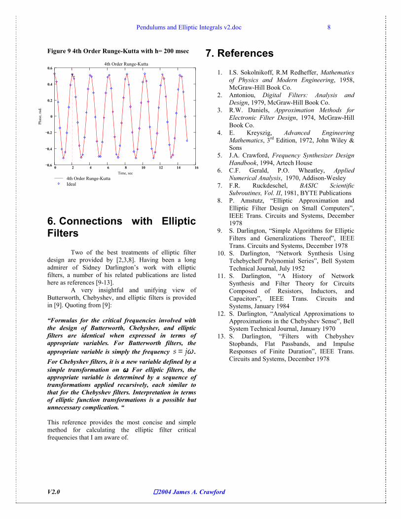
This set of difference equations is easily programmed and the results are shown for several time steps in Figure 7 through Figure 9. As shown in these figures, the computed results match the ideal results almost exactly even at the large time step of 200 msec. Although other techniques may be superior to the Runge-Kutta methods explored here, the simplicity of the method combined with the very good precision make it a highly recommended method for use in solving differential equations numerically.

Figure 7 4th Order Runge-Kutta with h= 30 msec

0 2 4 6 8 10 12 14 160.6

0.4

0.2

0

0.2

0.4

0.6

4th Order Runge-KuttaIdeal

4th Order Runge-Kutta

Time, sec

Phas

e, ra

d.

Tp


0 2 4 6 8 10 12 14 160.6

0.4

0.2

0

0.2

0.4

0.6



Time, sec

Phas

e, ra

d.

Tp




0 2 4 6 8 10 12 14 160.6

0.4

0.2

0

0.2

0.4

0.6



Time, sec

Phas

e, ra

d.

Tp

6. Connections with Elliptic Filters

Two of the best treatments of elliptic filter design are provided by [2,3,8]. Having been a long admirer of Sidney Darlington’s work with elliptic filters, a number of his related publications are listed here as references [9-13].

A very insightful and unifying view of Butterworth, Chebyshev, and elliptic filters is provided in [9]. Quoting from [9]:

“Formulas for the critical frequencies involved with the design of Butterworth, Chebyshev, and elliptic filters are identical when expressed in terms of appropriate variables. For Butterworth filters, the appropriate variable is simply the frequency s jω= . For Chebyshev filters, it is a new variable defined by a simple transformation on ωωωω. For elliptic filters, the appropriate variable is determined by a sequence of transformations applied recursively, each similar to that for the Chebyshev filters. Interpretation in terms of elliptic function transformations is a possible but unnecessary complication. “ This reference provides the most concise and simple method for calculating the elliptic filter critical frequencies that I am aware of.

7. References

1. I.S. Sokolnikoff, R.M Redheffer, Mathematics of Physics and Modern Engineering, 1958, McGraw-Hill Book Co.

2. Antoniou, Digital Filters: Analysis and Design, 1979, McGraw-Hill Book Co.

3. R.W. Daniels, Approximation Methods for Electronic Filter Design, 1974, McGraw-Hill Book Co.

4. E. Kreyszig, Advanced Engineering Mathematics, 3rd Edition, 1972, John Wiley & Sons

5. J.A. Crawford, Frequency Synthesizer Design Handbook, 1994, Artech House

6. C.F. Gerald, P.O. Wheatley, Applied Numerical Analysis, 1970, Addison-Wesley

7. F.R. Ruckdeschel, BASIC Scientific Subroutines, Vol. II, 1981, BYTE Publications

8. P. Amstutz, “Elliptic Approximation and Elliptic Filter Design on Small Computers”, IEEE Trans. Circuits and Systems, December 1978

9. S. Darlington, “Simple Algorithms for Elliptic Filters and Generalizations Thereof”, IEEE Trans. Circuits and Systems, December 1978

10. S. Darlington, “Network Synthesis Using Tchebycheff Polynomial Series”, Bell System Technical Journal, July 1952

11. S. Darlington, “A History of Network Synthesis and Filter Theory for Circuits Composed of Resistors, Inductors, and Capacitors”, IEEE Trans. Circuits and Systems, January 1984

12. S. Darlington, “Analytical Approximations to Approximations in the Chebyshev Sense”, Bell System Technical Journal, January 1970

13. S. Darlington, “Filters with Chebyshev Stopbands, Flat Passbands, and Impulse Responses of Finite Duration”, IEEE Trans. Circuits and Systems, December 1978

Advanced Phase-Lock Techniques

James A. Crawford

2008

Artech House

510 pages, 480 figures, 1200 equations

CD-ROM with all MATLAB scripts

ISBN-13: 978-1-59693-140-4 ISBN-10: 1-59693-140-X

Chapter Brief Description Pages

1 Phase-Locked Systems—A High-Level Perspective An expansive, multi-disciplined view of the PLL, its history, and its wide application.

26

2 Design Notes A compilation of design notes and formulas that are developed in details separately in the text. Includes an exhaustive list of closed-form results for the classic type-2 PLL, many of which have not been published before.

44

3 Fundamental Limits A detailed discussion of the many fundamental limits that PLL designers may have to be attentive to or else never achieve their lofty performance objectives, e.g., Paley-Wiener Criterion, Poisson Sum, Time-Bandwidth Product.

38

4 Noise in PLL-Based Systems An extensive look at noise, its sources, and its modeling in PLL systems. Includes special attention to 1/f noise, and the creation of custom noise sources that exhibit specific power spectral densities.

66

5 System Performance A detailed look at phase noise and clock-jitter, and their effects on system performance. Attention given to transmitters, receivers, and specific signaling waveforms like OFDM, M-QAM, M-PSK. Relationships between EVM and image suppression are presented for the first time. The effect of phase noise on channel capacity and channel cutoff rate are also developed.

48

6 Fundamental Concepts for Continuous-Time Systems A thorough examination of the classical continuous-time PLL up through 4th-order. The powerful Haggai constant phase-margin architecture is presented along with the type-3 PLL. Pseudo-continuous PLL systems (the most common PLL type in use today) are examined rigorously. Transient response calculation methods, 9 in total, are discussed in detail.

71

7 Fundamental Concepts for Sampled-Data Control Systems A thorough discussion of sampling effects in continuous-time systems is developed in terms of the z-transform, and closed-form results given through 4th-order.

32

8 Fractional-N Frequency Synthesizers A historic look at the fractional-N frequency synthesis method based on the U.S. patent record is first presented, followed by a thorough treatment of the concept based on ∆-Σ methods.

54

9 Oscillators An exhaustive look at oscillator fundamentals, configurations, and their use in PLL systems.

62

10 Clock and Data Recovery Bit synchronization and clock recovery are developed in rigorous terms and compared to the theoretical performance attainable as dictated by the Cramer-Rao bound.

52

Phase-Locked Systems—A High-Level Perspective 3

are described further for the ideal type-2 PLL in Table 1-1. The feedback divider is normally present only in frequency synthesis applications, and is therefore shown as an optional element in this figure.

PLLs are most frequently discussed in the context of continuous-time and Laplace transforms. A clear distinction is made in this text between continuous-time and discrete-time (i.e., sampled) PLLs because the analysis methods are, rigorously speaking, related but different. A brief introduction to continuous-time PLLs is provided in this section with more extensive details provided in Chapter 6.

PLL type and PLL order are two technical terms that are frequently used interchangeably even though they represent distinctly different quantities. PLL type refers to the number of ideal poles (or integrators) within the linear system. A voltage-controlled oscillator (VCO) is an ideal integrator of phase, for example. PLL order refers to the order of the characteristic equation polynomial for the linear system (e.g., denominator portion of (1.4)). The loop-order must always be greater than or equal to the loop-type. Type-2 third- and fourth-order PLLs are discussed in Chapter 6, as well as a type-3 PLL, for example.

dKrefθ

PhaseDetector

LoopFilter

VCO

FeedbackDivider

1N

outθ

Figure 1-2 Basic PLL structure exhibiting the basic functional ingredients.

Table 1-1

Basic Constitutive Elements for a Type-2 Second-Order PLL Block Name Laplace Transfer Function Description

Phase Detector Kd, V/rad Phase error metric that outputs a voltage that is proportional to the phase error existing between its input θref and the feedback phase θout/N. Charge-pump phase detectors output a current rather than a voltage, in which case Kd has units of A/rad.

Loop Filter 2

1

1 ss

ττ

+

Also called the lead-lag network, it contains one ideal pole and one finite zero.

VCO vK

s

The voltage-controlled oscillator (VCO) is an ideal integrator of phase. Kv normally has units of rad/s/V.

Feedback Divider 1/N A digital divider that is represented by a continuous divider of phase in the continuous-time description.

The type-2 second-order PLL is arguably the workhorse even for modern PLL designs. This PLL

is characterized by (i) its natural frequency ωn (rad/s) and (ii) its damping factor ζ. These terms are used extensively throughout the text, including the examples used in this chapter. These terms are separately discussed later in Sections 6.3.1 and 6.3.2. The role of these parameters in shaping the time- and frequency-domain behavior of this PLL is captured in the extensive list of formula provided in Section 2.1. In the continuous-time-domain, the type-2 second-order PLL3 open-loop gain function is given by

3 See Section 6.2.

4 Advanced Phase-Lock Techniques

( )2

2

1

1nOL

sG s

s sω τ

τ+ =

(1.1)

and the key loop parameters are given by

1

d vn

K KN

ωτ

= (1.2)

2

12 nζ ω τ= (1.3)

The time constants τ1 and τ2 are associated with the loop filter’s R and C values as developed in Chapter 6. The closed-loop transfer function associated with this PLL is given by the classical result

( ) ( )( )

2

1 2 2

21

12

nnout

ref n n

ss

H sN s s s

ζωωθ

θ ζω ω

+

= =+ +

(1.4)

The transfer function between the synthesizer output phase noise and the VCO self-noise is given by H2(s) where

( ) ( )2 11H s H s= − (1.5)

A convenient frequency-domain description of the open-loop gain function is provided in Figure

1-3. The frequency break-points called out in this figure and the next two appear frequently in PLL work and are worth committing to memory. The unity-gain radian frequency is denoted by ωu in this figure and is given by

2 42 4 1u nω ω ζ ζ= + + (1.6) A convenient approximation for the unity-gain frequency (1.6) is given by ωu ≅ 2ζωn. This result is accurate to within 10% for ζ ≥ 0.704.

The H1(s) transfer function determines how phase noise sources appearing at the PLL input are conveyed to the PLL output and a number of other important quantities. Normally, the input phase noise spectrum is assumed to be spectrally flat resulting in the output spectrum due to the reference noise being shaped entirely by |H1(s)|2. A representative plot of |H1|

2 is shown in Figure 1-4. The key frequencies in the figure are the frequency of maximum gain, the zero dB gain frequency, and the –3 dB gain frequency which are given respectively by

211 8 1 Hz

2 2n

PkFω ζ

π ζ= + − (1.7)

0

12 Hz

2dB nF ωπ

= (1.8)

2 4 23

11 2 2 Hz

2 2n

dBFω ζ ζ ζπ

= + + + + (1.9)


Frequency, rad/sec1 102 3 5 7 2 3 5

Gai

n, d

B (

6 dB

/cm

) -12 dB/octave

-6 dB/octave

0 dB

4 2 21010log 4n nω ω ζ

+

nω uω

2nωζ

( )1040log 2.38ζ

Figure 1-3 Open-loop gain approximations for classic continuous-time type-2 PLL.

100

101

102

-12

-10

-8

-6

-4

-2

0

2

4

6

Frequency, Hz

Gai

n, d

B

H1 Closed-Loop Gain

GPkF3dB

F0dB

FPk

Asymptotic-6 dB/octave

Figure 1-4 Closed-loop gain H1( f ) for type-2 second-order PLL4 from (1.4). The amount of gain-peaking that occurs at frequency Fpk is given by

4

10 4 2 2

810log dB

8 4 1 1 8PkG

ζζ ζ ζ

= − − + +

(1.10)

For situations where the close-in phase noise spectrum is dominated by reference-related phase noise, the amount of gain-peaking can be directly used to infer the loop’s damping factor from (1.10), and the 4 Book CD:\Ch1\u14033_figequs.m, ζ = 0.707, ωn = 2π 10 Hz.


loop’s natural frequency from (1.7). Normally, the close-in (i.e., radian offset frequencies less than ωn /2ζ) phase noise performance of a frequency synthesizer is entirely dominated by reference-related phase noise since the VCO phase noise generally increases 6 dB/octave with decreasing offset frequency5 whereas the open-loop gain function exhibits a 12 dB/octave increase in this same frequency range.

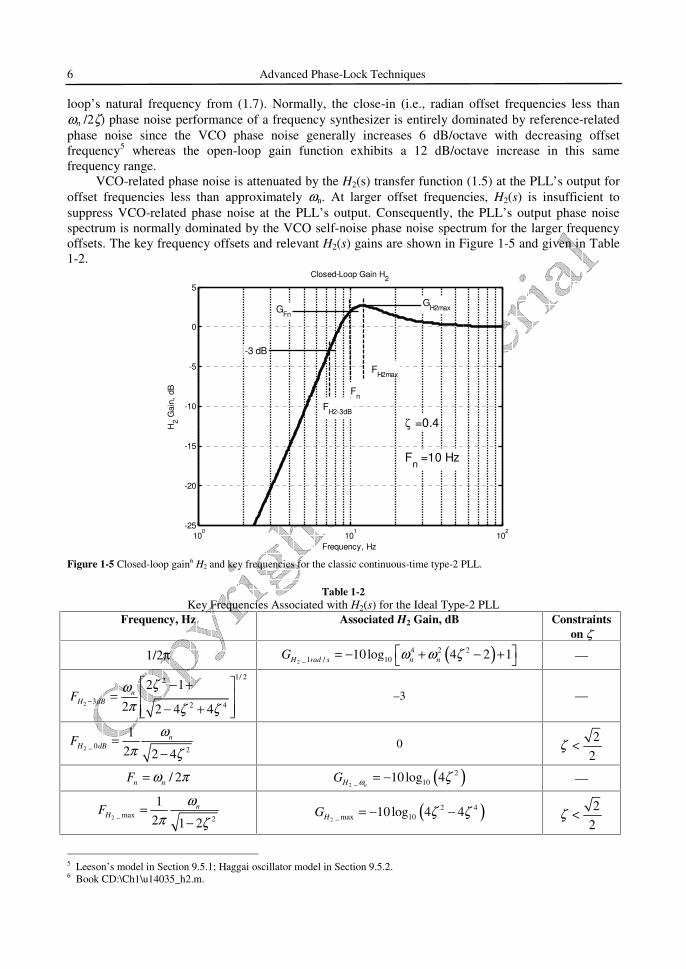
VCO-related phase noise is attenuated by the H2(s) transfer function (1.5) at the PLL’s output for offset frequencies less than approximately ωn. At larger offset frequencies, H2(s) is insufficient to suppress VCO-related phase noise at the PLL’s output. Consequently, the PLL’s output phase noise spectrum is normally dominated by the VCO self-noise phase noise spectrum for the larger frequency offsets. The key frequency offsets and relevant H2(s) gains are shown in Figure 1-5 and given in Table 1-2.

100

101

102

-25

-20

-15

-10

-5

0

5

Frequency, Hz

H2 G

ain,

dB

Closed-Loop Gain H2

ζ =0.4

Fn =10 Hz

-3 dB

FH2-3dB

Fn

GFnGH2max

FH2max

Figure 1-5 Closed-loop gain6 H2 and key frequencies for the classic continuous-time type-2 PLL.

Table 1-2 Key Frequencies Associated with H2(s) for the Ideal Type-2 PLL

Frequency, Hz Associated H2 Gain, dB Constraints on ]

1/2π ( )2

4 2 2_1 / 1010log 4 2 1H rad s n nG ω ω ζ = − + − + —

2

1/ 22

3 2 4

2 1

2 2 4 4n

H dBFζω

π ζ ζ−

− +=

− + –3 —

2 _ 0 2

12 2 4

nH dBF

ωπ ζ

=−

0 22

ζ <

/ 2n nF ω π= ( )2

2_ 1010log 4

nHG ω ζ= − —

2 _ max 2

12 1 2

nHF

ωπ ζ

=−

( )2

2 4_ max 1010log 4 4HG ζ ζ= − − 2

2ζ <

5 Leeson’ s model in Section 9.5.1; Haggai oscillator model in Section 9.5.2. 6 Book CD:\Ch1\u14035_h2.m.


Assuming that the noise samples have equal variances and are uncorrelated, R = σn2I where I is the

K×K identity matrix. In order to maximize (1.43) with respect to θ, a necessary condition is that the derivative of (1.43) with respect to θ be zero, or equivalently

( )

( ) ( )

2cos 0

2 cos sin 0

k o kk

k o k o kk

Lr A t

r A t A t

ω θθ θ

ω θ ω θ

∂ ∂= − + = ∂ ∂= − + + =

∑∑

(1.44)

Simplifying this result further and discarding the double-frequency terms that appear, the maximum-likelihood estimate for θ is that value that satisfies the constraint

( )kˆsin 0k o kk

r tω θ+ =∑ (1.45)

The top line indicates that double-frequency terms are to be filtered out and discarded. This result is equivalent to the minimum-variance estimator just derived in (1.40).

Under the assumed linear Gaussian conditions, the minimum-variance (MV) and maximum-likelihood (ML) estimators take the same form when implemented with a PLL. Both algorithms seek to reduce any quadrature error between the estimate and the observation data to zero.

1.4.3 PLL as a Maximum A Posteriori (MAP)-Based Estimator

The MAP estimator is used for the estimation of random parameters whereas the maximum-likelihood (ML) form is generally associated with the estimation of deterministic parameters. From Bayes rule for an observation z, the a posteriori probability density is given by

( ) ( ) ( )( )

p z pp z

p z

θ θθ = (1.46)

and this can be re-written in the logarithmic form as

( ) ( ) ( ) ( )log log log loge e e ep z p z p p zθ θ θ = + − (1.47)

This log-probability may be maximized by setting the derivative with respect to θ to zero thereby creating the necessary condition that27

( ) ( ){ } ˆlog log 0

MAPe e

dp z p

d θ θθ θ

θ = + = (1.48)

If the density p(θ ) is not known, the second term in (1.48) is normally discarded (set to zero) which degenerates naturally to the maximum-likelihood form as

( ){ } ˆlog 0

MLe

dp z

d θ θθ

θ = = (1.49)

27 [15] Section 6.2.1, [17] Section 2.4.1, [18] Section 5.4, and [22].


Time of Peak Phase-Error with Frequency-Step Applied 2

1

2

11tan

1fstep

n

Tζ

ζω ζ−

− = −

Note.1 See Figure 2-19 and Figure 2-20.

(2.29)

Time of Peak Phase-Error with Phase-Step Applied

( )2

1 2 2 1

2 2

11 2tan 2 1 ,2 1 tan

1 1step

n n

Tθζ

ζ ζ ζζω ζ ω ζ

− − − = − − = − −

See Figure 2-19 and Figure 2-20.

(2.30)

Time of Peak Frequency-Error with Phase-Step Applied

2

1:

1 211 :2

u

pk

nu

Tζ θ

ω ζ ζ θ π

≤= − > +

with ( )1 2 2 3tan 1 4 1 ,3 4uθ ζ ζ ζ ζ− = − − −

See Figure 2-21 and Figure 2-22. Tpk corresponds to the first point in time where dfo/dt = 0.

(2.31) (2.32)

Maximum Frequency-Error with Phase-Step Applied Use (2.31) in (2.28). (2.33) Time of Peak Frequency-Error with Frequency-Step Applied 2

1

2

12tan

1pk

n

Tζ

ζω ζ−

− = −

(2.34)

% Transient Frequency Overshoot for Frequency-Step Applied

( ) ( )2 2% 2

cos 1 sin 1 100%1

n pkTn pk n pkOS T T e ζωζζ ω ζ ω

ζ−

= − − − ×

−

21

2

12tan

1pk

n

Tζ

ζω ζ−

− = −

Note.2 See Figure 2-23 and Figure 2-24.

(2.35) (2.36)

Linear Hold-In Range with Frequency-Step Applied (Without Cycle-Slip) 2

1max 2

1exp tan Hz

1nF

ζζωζζ

− − ∆ =

−

See Figure 2-25.

(2.37)

Linear Settling Time with Frequency-Step Applied (Without Cycle-Slip) (Approx.)

2

1 1log sec

1Lock e

n

FT

Fζω δ ζ

∆ ≤ −

for applied frequency-step of ∆F and residual δ F remaining at lock See Figure 2-26.

(2.38)

1 The peak occurrence time is precisely one-half that given by (2.34). 2 See Figure 2-24 for time of occurrence Tpk for peak overshoot/undershoot with ωn = 2π. Amount of overshoot/undershoot in percent provided in Figure 2-23.


2.3.2.2 Second-Order Gear Result for H1(z) for Ideal Type-2 PLL

θe

Σθin

+ -

D

+

_ θo

+

ΣD

31n sTζ

ω+

n sTζ

ω

4n sTζ

ω

Σ

v

Σ

+_

+

D

23

sT

43 D

13

Σ

+_

+

D

223

sn

T ω

43 D

13

Figure 2-32 Second-order Gear redesign of H1(s) (2.4).

( )1 2

2

21 2

3 4 11 1

2 3 33 4 1

13 3

n s n sOL

z zT T

G z

z z

ζω ω

− −

− −

+ − + = − +

(2.52)

( ) ( ) ( ) ( )2 2 4

0 0 1

1o n in n n o

n n n

k a k n b v k n c k nD

θ θ θ= = =

= − + − + − ∑ ∑ ∑ (2.53)

0

1

2

31

4n s

n s

n s

aT

aT

aT

ζωζ

ωζ

ω

= +

= −

=

(2.54)

0 2

1 2

2 2

32

2

12

n s

n s

n s

bT

bT

bT

ω

ω

ω

=

= −

=

(2.55)

( )

( )

( )

( )

1 2

2 2

3 2

4 2

6 4

11

2

2

1

2

n sn s

n sn s

n s

n s

cTT

cTT

cT

cT

ζωω

ζωω

ω

ω

= +

= − −

=

= −

(2.56)

23 3

12n s n s

DT Tζ

ω ω

= + +

(2.57)

2.3.3 Higher-Order Differentiation Formulas

In cases where a precision first-order time-derivative f (xn+1) must be computed from an equally spaced sample sequence, higher-order formulas may be helpful.8 Several of these are provided here in Table 2-2. The uniform time between samples is represented by Ts.

8 Precisions compared in Book CD:\Ch2\u14028_diff_forms.m.


2.5.5 64-QAM Symbol Error Rate

15 16 17 18 19 20 21 22 23 24 2510

-8

10-7

10-6

10-5

10-4

10-3

10-2

Eb/No, dB

SE

R

64-QAM Symbol Error Rate

σφ = 2o rms

σφ = 1.5o rms

σφ = 1o rms

σφ = 0.5o rms

No Phase Noise

Proakis

Figure 2-37 64-QAM uncoded symbol error rate with noisy local oscillator.13 Circled datapoints are from (2.87).

13 Book CD:\Ch5\u13159_qam_ser.m. See Section 5.5.3 for additional information. Circled datapoints are based on Proakis [3] page 282, equation (4.2.144), included in this text as (2.87).

Fundamental Limits 83

A more detailed discussion of the Chernoff bound and its applications is available in [9].

Key Point: The Chernoff bound can be used to provide a tight upper-bound for the tail-probability of a one-sided probability density. It is a much tighter bound than the Chebyschev inequality given in Section 3.5. The bound given by (3.43) for the complementary error function can be helpful in bounding other performance measures.

3.7 CRAMER-RAO BOUND

The Cramer-Rao bound16 (CRB) was first introduced in Section 1.4.4, and frequently appears in phase- and frequency-related estimation work when low SNR conditions prevail. Systems that asymptotically achieve the CRB are called efficient in estimation theory terminology. In this text, the CRB is used to quantify system performance limits pertaining to important quantities such as phase and frequency estimation, signal amplitude estimation, bit error rate, etc.

The CRB is used in Chapter 10 to assess the performance of several synchronization algorithms with respect to theory. Owing to the much larger signal SNRs involved with frequency synthesis, however, the CRB is rarely used in PLL-related synthesis work. The CRB is developed in considerable detail in the sections that follow because of its general importance, and its widespread applicability to the analysis of many communication system problems.

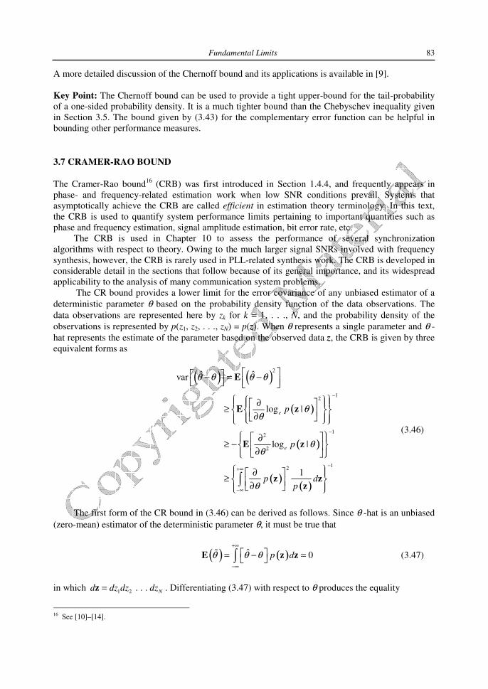
The CR bound provides a lower limit for the error covariance of any unbiased estimator of a deterministic parameter θ based on the probability density function of the data observations. The data observations are represented here by zk for k = 1, . . ., N, and the probability density of the observations is represented by p(z1, z2, . . ., zN) = p(z). When θ represents a single parameter and θ -hat represents the estimate of the parameter based on the observed data z, the CRB is given by three equivalent forms as

( ) ( )

( )

( )

( ) ( )

2

12

12

2

12

ˆ ˆvar

log |

log |

1

e

e

p

p

p dp

θ θ θ θ

θθ

θθ

θ

−

−

−+∞

−∞

− = −

∂ ≥ ∂

∂ ≥ − ∂

∂ ≥ ∂ ∫

E

E z

E z

z zz

(3.46)

The first form of the CR bound in (3.46) can be derived as follows. Since θ -hat is an unbiased

(zero-mean) estimator of the deterministic parameter θ, it must be true that

( ) ( )ˆ 0p dθ θ θ+∞

−∞

= − = ∫E z z� (3.47)

in which 1 2 . . . Nd dz dz dz=z . Differentiating (3.47) with respect to θ produces the equality

16 See [10]–[14].


{ }2

ˆvar for all casesobMσ≥ (3.62)

{ }

( )

2

20

2

2 20

Phase known, amplitude known or unknown

ˆvar12

Phase unknown, amplitude known or unknownb 1

o s

b QT

M M

σ

ωσ

≥ −

(3.63)

{ }( )

2

20

2

2 2 20

Frequency known, amplitude known or unknownˆvar

12Frequency unknown, amplitude known or unknown

1

o

b M

Q

b M M

σ

θσ

≥ −

(3.64)

In the formulation presented by (3.55), the signal-to-noise ratio ρ is given by ρ = b0

2 / (2σ 2). For the present example, the CR bound is given by the top equation in (3.63) and is as shown

in Figure 3-9 when the initial signal phase θo is known a priori. Usually, the carrier phase θo is not known a priori when estimating the signal frequency, however, and the additional unknown parameter causes the estimation error variance to be increased, making the variance asymptotically 4-times larger than when the phase is known a priori. This CR variance bound for this more typical unknown signal phase situation is shown in Figure 3-10.

Beginning with (3.57), a maximum-likelihood17 frequency estimator can be formulated as described in Appendix 3A. It is insightful to compare this estimator’s performance with its respective CR bound. For simplicity, the initial phase θo is assumed to be random but known a priori. The results for M = 80 are shown in Figure 3-11 where the onset of thresholding is apparent for ρ ≅ –2 dB. Similar results are shown in Figure 3-12 for M = 160 where the threshold onset has been improved to about ρ ≅ –5 dB.

100

101

102

103

10-7

10-6

10-5

10-4

10-3

10-2

10-1

100

Number of Samples

Est

imat

or V

aria

nce,

var

( ω oT

)

CR Bound for Frequency Estimation Error Variance

ρ = -20 dB

ρ = -10 dB

ρ = 0 dB

ρ = 10 dB

ρ = 20 dB

Figure 3-9 CR bound18 for frequency estimation error with phase θo known a priori (3.63).

17 See Section 1.4.2. 18 Book CD:\Ch3\u13000_crb.m. Amplitude known or unknown, frequency unknown, initial phase known.

Noise in PLL-Based Systems 135

would be measured and displayed on a spectrum analyzer. Having recognized the carrier and continuous spectrum portions within (4.65), it is possible to equate29

( ) ( ) 2rad /Hzf P fθ≅/ (4.66)

Frequency

( )12 oP fθ ν−

Carrier

oνxf

( )xf/

oν−

Power

Figure 4-17 Resultant two-sided power spectral density from (4.65), and the single-sideband-to-carrier ratio

�( f ).

Both /( f ) and Pθ ( f ) are two-sided power spectral densities, being defined for positive as well as negative frequencies.

The use of one-sided versus two-sided power spectral densities is a frequent point of confusion in the literature. Some PSDs are formally defined only as a one-sided density. Two-sided power spectral densities are used throughout this text (aside from the formal definitions for some quantities given in Section 4.6.1) because they naturally occur when the Wiener-Khintchine relationship is utilized.

4.6.1 Phase Noise Spectrum Terminology

A minimum amount of standardized terminology has been used thus far in this chapter to characterize phase noise quantities. In this section, several of the more important formal definitions that apply to phase noise are provided.

A number of papers have been published which discuss phase noise characterization fundamentals [34]–[40]. The updated recommendations of the IEEE are provided in [41] and those of the CCIR in [42]. A collection of excellent papers is also available in [43].

In the discussion that follows, the nominal carrier frequency is denoted by νo (Hz) and the frequency-offset from the carrier is denoted by f (Hz) which is sometimes also referred to as the Fourier frequency.

One of the most prevalent phase noise spectrum measures used within industry is /( f ) which was encountered in the previous section. This important quantity is defined as [44]:

/( f ): The normalized frequency-domain representation of phase fluctuations. It is the ratio of the power spectral density in one phase modulation sideband, referred to the carrier frequency on a spectral density basis, to the total signal power, at a frequency offset f. The units30 for this quantity are Hz–1. The frequency range for f ranges from –νo to ∞. /( f ) is therefore a two-sided spectral density and is also called single-sideband phase noise.

29 It implicitly assumed that the units for

�( f ), dBc/Hz or rad2/Hz, can be inferred from context.

30 Also as rad2/Hz.

Noise in PLL-Based Systems 163

exp2i iz p pα = ∆

(4B.10)

A minimum of one filter section per frequency decade is recommended for reasonable accuracy. A sample result using this method across four frequency decades using 3 and 5 filter sections is shown in Figure 4B-3.

100

101

102

103

104

105

0

5

10

15

20

25

30

35

40

45

Radian Frequency

Rel

ativ

e S

pect

rum

Lev

el, d

B

f -α Power Spectral Density

5 Filter Sections

3 Filter Sections

α = 1

Figure 4B-3 1/f noise creation using recursive 1/f 2 filtering method4 with white Gaussian noise.

1/f �

Noise Generation Using Fractional-Differencing Methods

Hosking [6] was the first to propose the fractional differencing method for generating 1/f α noise. As pointed out in [3], this approach resolves many of the problems associated with other generation methods. In the continuous-time-domain, the generation of 1/f α noise processes involves the application of a nonrealizable filter to a white Gaussian noise source having s–α/2 for its transfer function. Since the z-transform equivalent of 1/s is H(z) = (1 – z–1)–1, the fractional digital filter of interest here is given by

( )( ) / 21

1

1H z

zα α−

=−

(4B.11)

A straightforward power series expansion of the denominator can be used to express the filter as an infinite IIR filter response that uses only integer-powers of z as

( )

1

1 2

12 21 . . .

2 2!H z z zα

α αα

−

− −

− ≈ − − −

(4B.12)

in which the general recursion formula for the polynomial coefficients is given by

4 Book CD:\Ch4\u13070_recursive_flicker_noise.m.

System Performance 185

dBL∆

SepF∆

StrongInterferer

DesiredChannel

Local OscillatorSpectrum

SepF∆

SidebandNoise

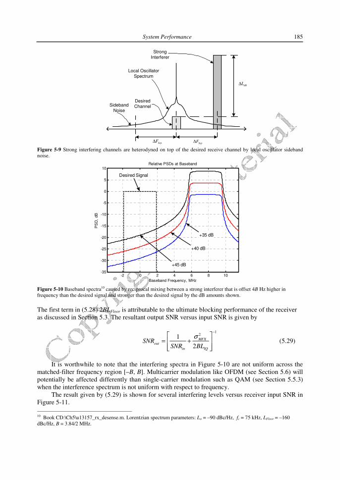
Figure 5-9 Strong interfering channels are heterodyned on top of the desired receive channel by local oscillator sideband noise.

-2 0 2 4 6 8 10-35

-30

-25

-20

-15

-10

-5

0

5

10

Baseband Frequency, MHz

PS

D,

dB

Relative PSDs at Baseband

Desired Signal

+35 dB

+40 dB

+45 dB

Figure 5-10 Baseband spectra10 caused by reciprocal mixing between a strong interferer that is offset 4B Hz higher in frequency than the desired signal and stronger than the desired signal by the dB amounts shown. The first term in (5.28) 2BLFloor is attributable to the ultimate blocking performance of the receiver as discussed in Section 5.3. The resultant output SNR versus input SNR is given by

1

212

MFXout

in IQ

SNRSNR BL

σ−

= +

(5.29)

It is worthwhile to note that the interfering spectra in Figure 5-10 are not uniform across the

matched-filter frequency region [–B, B]. Multicarrier modulation like OFDM (see Section 5.6) will potentially be affected differently than single-carrier modulation such as QAM (see Section 5.5.3) when the interference spectrum is not uniform with respect to frequency.

The result given by (5.29) is shown for several interfering levels versus receiver input SNR in Figure 5-11. 10 Book CD:\Ch5\u13157_rx_desense.m. Lorentzian spectrum parameters: Lo = –90 dBc/Hz, fc = 75 kHz, LFloor = –160 dBc/Hz, B = 3.84/2 MHz.

System Performance 221

of 3° rms phase noise is shown in Figure 5B-8. The tail probability is worse than the exact computations shown in Figure 5-17 but the two results otherwise match very well.

5 7 9 11 13 15 17 19 202.2

2.4

2.6

2.8

3

3.2

3.4

3.6

3.8

4

Eb/No, dB

Bits

per

Sym

bol

Channel Cutoff Rate Ro

10o

8o6o

4o

0o

Figure 5B-6 Channel cutoff rate,7 Ro, for 16-QAM with static phase errors as shown, from (5B.16).

1 3 5 7 9 11 13 15 17 19 21 231.5

1.75

2

2.25

2.5

2.75

3

3.25

3.5

3.75

4

Eb/No, dB

Bits

per

Sym

bol

Channel Cutoff Rate Ro Including Phase Noise

Figure 5B-7 Ro for8 16-QAM versus Eb/No for 5° rms phase noise from (5B.18) (to accentuate loss in Ro even at high SNR values). 7 Book CD:\Ch5\u13176_rolo.m. 8 Ibid.

Fractional-N Frequency Synthesizers 371

required, however, because the offset current will introduce its own shot-current noise contribution, and the increased duty-cycle of the charge-pump activity will also introduce additional noise and potentially higher reference spurs. Single-bit ∆-Σ modulators are attractive in this respect because they lead to the minimum-width phase-error distribution possible.

PDθ

CPIIdeal

Figure 8-70 Charge-pump (i) dead-zone and (ii) unequal positive versus negative error gain.

103

104

105

106

107

-140

-130

-120

-110

-100

-90

-80

-70

-60

-50

-40

Frequency, Hz

Pha

se N

oise

, dB

c/H

z

MASH 2-2 Output Spectrum with Nonlinear PD

Figure 8-71 Phase error power spectral density48 for the MASH 2-2 ∆-Σ modulator shown in Figure 8-55 with M = 222, P = M/2 + 3,201, and 2% charge-pump gain imbalance. Increased noise floor and discrete spurs are clearly apparent compared to Figure 8-56.

Classical random processes theory can be used to provide several useful insights about nonlinear phase detector operation. In the case of unequal positive-error versus negative-error phase detector gain, the memoryless nonlinearity can be modeled as

( )0pd in in inθ φ α φ φ= + > (8.39) where α represents the additional gain that is present for positive phase errors. The instantaneous phase error due to the modulator’s internal quantization creates a random phase error sequence that can be represented by 48 Book CD:\Ch8\u12735_MASH2_2_nonlinear.m.

Clock and Data Recovery 457

the sampling-point within each symbol-period after the datalink signal has been fully acquired. In the example results that follow, the data source is assumed to be operating at 1 bit-per-second, utilizing square-root raised-cosine pulse-shaping with an excess bandwidth parameter β = 0.50 at the transmitter. The eye-diagram of the signal at the transmit end is shown in Figure 10-15. The ideal matched-filter function in the CDR is closely approximated by an N = 3 Butterworth lowpass filter having a –3 dB corner frequency of 0.50 Hz like the filter used in Section 10.4. The resulting eye-diagram at the matched-filter output is shown in Figure 10-16 for Eb/No = 25 dB.

MatchedFilter

( )MFH f

Sample Gate

VCO LoopFilter

( )A t

( ) ( )2 MFj f H fπ

( )y t ( )fy t

( )B t

( )2tanh f

o

y tN

lka

( )v t

Sample Gate

Figure 10-14 ML-CDR implemented with continuous-time filters based on the timing-error metric given by (10.21).

-1 -0.5 0 0.5 1-1.5

-1

-0.5

0

0.5

1

1.5

Time, Symbols

Nor

mal

ized

Square-Root Raised-Cosine Eye-Diagram

Figure 10-15 Eye diagram15 at the data source output assuming square-root raised-cosine pulse shaping with an excess bandwidth parameter β = 0.50.

A clear understanding of the error metric represented by v(t) in Figure 10-14 is vital for understanding how the CDR operates. The metric is best described by its S-curve behavior versus input Eb/No as shown in Figure 10-17. Each curve is created by setting the noise power spectral density No for a specified Eb/No value with Eb = 1, and computing the average of v( kTsym+ ε ) for k = [0, K] as the timing-error ε is swept across [0, Tsym]. The slope of each S-curve near the zero-error steady-state tracking value determines the linear gain of the metric that is needed to compute the closed-loop bandwidth, loop stability margin, and other important quantities. For a given input SNR, 15 Book CD:\Ch10\u14004_ml_cdr.m.


the corresponding S-curve has only one timing-error value εo for which the error metric value is zero and the S-curve slope has the correct polarity. As the gain value changes with input Eb/No, the closed-loop parameters will also vary. For large gain variations, the Haggai loop concept explored in Section 6.7 may prove advantageous.

-1 -0.5 0 0.5 1-1.5

-1

-0.5

0

0.5

1

1.5

Time

Am

plitu

de

Eye Diagram at Matched-Filter Output

Figure 10-16 Eye diagram16 at the CDR matched-filter output for Eb/No = 25 dB corresponding to the data source shown in Figure 10-15 and using an N = 3 Butterworth lowpass filter with BT = 0.50 for the approximate matched-filter.

0 0.1 0.2 0.3 0.4 0.5 0.6 0.7 0.8 0.9 1-0.4

-0.3

-0.2

-0.1

0

0.1

0.2

0.3

0.4

Timing, symbols

V

S-Curves

0 dB

3 dB

6 dB9 dB

15 dB

Eb/No= 25 dB

Figure 10-17 S-curves17 versus Eb/No corresponding to Figure 10-16 and ideal ML-CDR shown in Figure 10-14. Eb = 1 is assumed constant.

A second important characteristic of the timing-error metric is its variance versus input Eb/No and static timing-error ε. For this present example, this information is shown in Figure 10-18. The variance understandably decreases as the input SNR is increased, and as the optimum time-alignment within each data symbol is approached. The variance of the recovered data clock σclk

2 can be closely estimated in terms of the tracking-point voltage-error variance from Figure 10-18 denoted by σve

2 (V2), the slope (i.e., gain) of the corresponding S-curve (Kte, V/UI) from Figure 10-17, the symbol rate Fsym (= 1/Tsym), and the one-sided closed-loop PLL bandwidth BL (Hz) as 16 Ibid. 17 Ibid.

Documents

Pendulums and Elliptic Integrals - AM1 LLC · Pendulums and Elliptic Integrals v2.doc 4 V2.0 2004 James A. Crawford solving differential equations because it is extremely simple to