Embed Size (px)
Citation preview
Computers Math. Applic. Vol. 33, No. 12, pp. 15-114, 1997 P e r g a m o n Copyright(~)1997 Elsevier Science Ltd
Printed in Great Britain. All rights reserved 0898-1221/97 $17.00 + 0.00
PIh S0898-1221(97)00091-6
Elliptic Integrals and the Schwarz-Christoffel Transformation
W . C . H A S S E N P F L U G Department of Mechanical Engineering, University of Stellenbosch
Stellenbosch, South Africa
(Received December 1996; accepted January 1997)
A b s t r a c t - - T h e real elliptic integrals of the first and second kind in Jacobi's normal form are computed efficiently, using the convolution number in conjunction with the method of Frobenius. For this purpose certain treatments of the Laurent series are included. Different regions of convergence on the real axis are determined, and for each one a different series is developed. The real elliptic integral of the third kind is solved within a limited parameter plane by the same method.
The integral of the Schwarz-Christoffel transformation is solved in the complex variable by complex convolution number algebra, using the unit disk as mapping region. Different regions of convergence of Frobenius, Laurent, and Taylor series are determined to cover the whole disk. The complex evaluation of the elliptic integral of the third kind is included. A Schwarz-Christoffel formula for an infinite periodic mapping is given. The solutions for exterior, interior, periodic, and cyclic polygons are separately treated. Examples of several polygon mappings are presented graphically, and compared with previous numerically integrated solutions.
The parameter problem is solved by the Newton-Raphson method, using a quotient matrix as approximation for the Jacobian matrix. The coordinate relations are simplified by using an overde- termined system. An exact analytical Jacobian matrix is computed, solving Leibniz' derivative of the Schwarz-Christoffel integral, and results are compared with the approximate quotient matrix method.
geywords- -Schwarz-Chr i s to f fe l transformation, Elliptic integrals, Conformal mapping, Convo- lution number, Series expansions.
1. I N T R O D U C T I O N
T h e Schwarz-Chr is tof fe l t r ans fo rma t ion (SCT) m a p s a po lygon on a ha l fp lane or a c i rcular disk.
T h e S C T is fo rmula t ed as an integral t h a t leads only in the s imples t cases to el l ipt ic integrals ; t he
genera l case is usua l ly considered unsolvable , in the sense t h a t it canno t be expressed in t e r m s
of wel l -known and t a b u l a t e d functions. T h e advancemen t in compu te r s t h a t has m a d e finite
difference and finite e lement so lu t ions poss ible can now be used to find the ana ly t i ca l so lu t ions ,
a lbe i t not in t h e res t r i c t ed classic sense.
A n a l y t i c a l m e t h o d s d o m i n a t e d in t he solut ion of phys ica l p rob lems from the beg inn ing of
ana lys i s centur ies ago. As p rob lems became more and more demand ing , ana ly t i ca l funct ions
were deve loped , resu l t ing in numerous special functions, recorded in m a t h e m a t i c a l t r ea t i ses and
handbooks . Yet the s t ruggle to formula te solu t ions in t e rms of known funct ions b e c a m e ha rde r
as accu ra t e so lu t ions of real p rob lems were demanded .
A l r e a d y f rom 1905, p rac t i ca l ly minded Car l Runge deve loped the numer ica l i n t eg ra t ion tech-
niques, rea l iz ing t h a t a genera l differential equa t ion will p r o b a b l y never be solved analy t ica l ly .
Since then , ana ly t i c and numer ica l m e t h o d s have always run paral lel . W i t h the adven t of t he
compu te r , numer ica l m e t h o d s have over taken ana ly t i ca l me thods , since a b o u t t he 1960's.
T h e Schwarz-Chris toffe l t r ans fo rma t ion was a popu l a r ana ly t ic tool in fluid p rob l ems wi th
po lygon boundar ies , in free s t r eaml ine problems, and in p lane elast ic sys tems. In t e re s t in t he
15

16 W.C. HASSENPFLUG
analytic solution of the SCT stopped around the 1960's, when analytical methods were overtaken
by purely numerical methods in the solution of partial differential equations. From here on, roads of numerical and analytical solution methods parted.
Along a different path of development, the computer has also been used to handle analytical
methods in what are called symbolic computer languages. Yet these still rely on classic well-known
analytic functions.
Since the 1970's, numerical methods have solved the SCT successfully 11,2]. One of the best
known and popular methods was developed by Trefethen 13], particularly well explained, also
discussed and advocated by Henrici [4 I. That method is developed as a computer package, called
SCPACK, which is freely available from its author. Variations and improvements of the numerical
solution continue to appear [5-8]. An improvement for elongated regions, using Trefethen's
numerical integration, is given in [9]. An application package with unlimited scope for MATLAB I
is given in [10].
The result is that the SCT is used more frequently again, but now in the fields of hybrid micro-
electronics [11], VLSI design [12], magnetics [13-15], microwave theory [16,17], electromagnetic
fields [18], but also in fracture mechanics [19]. Many of these workers use their own numerical
techniques, others use Trefethen's SCPACK, i.e., [11,12,19].
In this paper, we present an analytic method for the computation of elliptic integrals and the
solution of the SCT, turning the clock back by some 20 years. There does not seem to be a
need of a new method any more, but we present our method as an alternative method to use the
computer to achieve the analytical solution and its numerical evaluation. From the crossroads, we
turn the clock forward again on the alternate analytical path, by how much we cannot estimate
ourselves.
The analytical solution of a physical problem consists of selecting suitable functions from the set
that has been developed during the last three centuries, and then to determine the coefficients. To
evaluate, the functions need to be evaluated numerically. In the SCT the functions are generally
not available; they are actually new functions defined by the SCT. An efficient and general method
to evaluate such new functions is by expansion in Taylor series. Computations are done on the
sequence of coefficients which are regarded as a number, called convolution number [20]. The
operations on the sequences are treated as operations on a number with convolution algebra [20],
making the expansion problem a simple algebraic problem, easily implemented on a computer.
Different well-known routines for the computation of the three basic elliptic integrals, F(¢,/¢),
E(¢,k), /-/(¢,k), are available, notably in the handbooks [21,22] or in treatises on applica-
tions [23,24]. Much effort has been made to write more efficient routines, as in [25,26]. Some more
efficient ones were developed recently in [271, where many more references are given. To program
these may be quite an effort in itself, but it does not solve the problem if the elliptic integrals
are not one of the three basic types. In that case, the relations with the three basic types must
first be be found, as in the tables of [211 . But then those integrals may involve many times the
computational effort of one elliptic integral, the worst case occurring when the original integral is
expressed as infinite series of elliptic integrals. Using the convolution number as computational
tool, all elliptic integrals are solved directly by the same method.
The range of integration of elliptic integrals and the SCT approaches or includes singular points. Then the method of Frobenius produces an analytic solution near the singularity [28],
which is used in conjunction with the convolution number, as was suggested in [20]. The Frobe-
nius expansion is particularly well suited to singular points which are infinities, which are such a problem in numerical integration. For this purpose, the range of integration near, or includ-
ing, the known singular points must be partitioned into suitable regions of convergence for the practical application of series. It was previously suggested [29] that we can approximate to any required accuracy by using enough terms of a single central Taylor series. However, even a good
1MATLAB is a registered trademark of The MathWorks, Inc,
Elliptic Integrals 17
approximation would need a few thousand terms, and the singularities can still not be computed, even less so if they are infinities. I t is shown in the following how the convolution number is used
to develop additional Frobenius and Laurent series to cover the whole range efficiently. For each value of the parameters, the series can be developed easily on a personal computer. All corner- points are singularities and need Frobenius disks, except the special case c~ = - 1 and winding points, a -- - 2 . . . . But singularities need not be infinities, as suggested in [11].
For the real elliptic integral, a region on the real line is parti t ioned into line segments on which the chosen series converge. For the SCT, the unit disk is chosen as mapping region, so tha t the whole range can be covered by a finite number of circular convergence regions, the number of which depends on the number and position of the singular points on the circle. An efficient covering is then achieved by using Frobenius, Laurent, and Taylor series.
The relation of the coordinates of the polygon corners with the position of the singular points on the circle is called the parameter problem. This is solved by a Newton-Raphson iteration.
The solution is then available in analytical form, in the sense as described in [20].
2. P R E L I M I N A R I E S
2.1. B i n o m i a l T h e o r e m
I t is worthwhile to add the binomial formula to the convolution number routines of [20], because the SCT formula consists of factors which are binomials to some power. The binomial formula is
simpler than the general convolution routine tha t computes c , as described in [20], because the pointer convolution numbers in that routine are not needed for the simple binomial. Ordinary convolution numbers are then sufficient for the solution of the SCT.
Generally for
/ ( z ) _= (a0 + alz) = z . / , (2.1)
the coefficients are given by the recurrence formula
£ = al , for i = 1 , . . . , n . (2.2) i a0
2.2. L a u r e n t Se r i e s
There are many occasions where the Laurent series can be used to obtain a more efficient covering of a region within a range of interest than the Taylor series. We will therefore need symbols to include Laurent series in expansions, even though convolution algebra cannot be done on a sequence of Laurent coefficients [20]. For our purposes, the full-Laurent series is split into two half-infinite series, one of which is a half-infinite Laurent series, called half-Laurent series, and the other is a Taylor series. The half-Laurent series is then a Taylor series of the inverted variable.
We introduce the new symbol for the half-Laurent series, for numerical purposes truncated to n terms,
al a2 an - - + + . . . + - - = Z . a ( 2 . 3 ) Z - ~ Z n
with the definitions similar to the Taylor convolution number,
,~Z--- , z2 , . . . , ,
a = {al, a2 , . . . , an}, (2.5)

18 W . C . HASSENPFLUG
e ~
where we call the sequence a the Laurent number. In equation (2.3) it acts as a column vector. With the t ransformation s = l / z , the half-Laurent series can be expressed as a Taylor series
als + ass s + . . . + a,~s "~ = _S. a , (2.6)
where a is the Taylor convolution number, which is the same sequence as a but with a different meaning. I t is this meaning tha t distinguishes a and a; in particular, the differentiation and integration is different. Otherwise, the two numbers are stored the same way in a computer , and no negative subscripts are used.
The algebra of Laurent numbers is defined by the corresponding algebra of Taylor series, e.g., multiplication
~ ~ ~ Y (2 7) V . a × V . b = V . a *
is equivalent to the product of Taylor convolution numbers
Z . a x Z . - b = Z . a * b .
The distinction is only necessary if both Taylor and half-Laurent series occur in the same context. A full-Laurent series is then expressed as the sum of a half-Laurent series and a Taylor series
a l , + . . . + a l s a l l z n (2.8) z " " ~ " + z - F a 2 0 q - a 2 1 z - F a 2 2 z 2 -}- . . . -F a2n = ~ Z ' a l - } - _ Z ' a 2 ,
where the constant a0 is always taken into the Taylor series. Wha t happens typically in elliptic integrals and the SCT is tha t the function to be integrated
is given in factors a(z) = al(z)as(z) , of which the first par t is expanded in a half-Laurent series and the second in a Taylor series, both in z about same the point z = 0, which we express now
as
a(z) = al(z) x as(z) = Z . a l x Z . as , (2.9)
which has to be expressed as a single full-Laurent series
a t ( z ) × as (z ) = bt(z) + b2(z) = Z . + Z_. ---- b(z). (2.10)
Although the functions a(z) and b(z) are analytically the same, we give their different forms different names.
In contrast to the convolution number, each Laurent coefficient in equation (2.10) consists of an
infinite sum of the terms of a l and a s . The best we can do numerically is not to lose any of the products of the t runcated series tha t contribute to the product, which are shown in Figure 2.1.
The multiplication and partitioning in half-Laurent and Taylor coefficients of equation (2.10) is then done according to
k2
bl~ = ~-~alka2k_~, for i ---- il . . . . ,i2, (2.11) kl
where
il = max( l , 11 - ms) , i2 = max(0, ml - 12),
kl = max(/ t , Is + i), k2 = min(mt , ms + i),
and
k2
b2i -- E a l k a 2 k + i , for i -- i l , . . . , is, (2.12) kl

Elliptic Integrals 19
bl
A r m m l / "- ~ X :/~"£E/X Z YI, I%£ X Z ~
~ "_ 2 . / / I , E / Z Z r , 4 , E / X Z /
- - " /~ZY , '$1~. /ZZLE/Z7 ~ / "- / Z Y z$1'IZ Z Z r/I,t~. X Z /
_o ~ Z ://I,,5< X Z :/ I /~. X Z.,n
, 3 Io lololol . [ - [ * l . l , lo lolo[ol l Iml
t l t l m n
@2
Figure 2 . 1 . C o n v o l u t i o n n u m b e r multiplication a l * a 2 = [b l , b 2 ] .
where
il : max(0,12 - ml) , i2 = m ax ( -1 , m2 -- /1),
kl = max(/1,12 -- i), k2 = min(ml, m2 -- i),
and the pointers ll, ml , 12, m2 are taken from the numbers al and a2, see [20]. In Figure 2.1, the parts that contribute to the two different numbers are shown enclosed by
the thick lines. Note that in Figure 2.1 we have shown a with an empty space in the 0-position, according to equation (2.3), but we allow for an occupied position there before multiplication
e~ and separation, which occurs from the development of a by a binomial expansion.
Symbolically we express the operations of equations (2.11) and (2.12) by the notation
a l * - a 2 = b~, b2 , ( 2 . 1 3 )
or by the simpler symbol
al * a2 =~ b], b2. (2.14)
The relation between equations (2.13),(2.14) with (2.9) and (2.10) is formally expressed by
~ - ~ 1 - -~ ~ ( Z . a l x Z - a2 = Z . * a2 = Z . b = Z . bl + Z . b 2 . 2.15)
Contrary to convolution numbers, Laurent coefficients obtained by this method are not exact; each coefficient is defined by an infinite series.
20 W . C . HASSENPFLUG
The general integration of a half-Laurent series
a ( z ) = . . . . a l + a 2 a . ~ z ~ +" " + z n = Z a (2.16)
to b(z) = f a ( z ) d z results in
b(z) = at log z + -a2 .{_ 1 -a3 1 -gn z + " " +
-- a l l o g z + --blz + ~.~+...+b2 ~ z n-lbn-1 = a l l o g z + Z . b , (2.17)
so that the coefficients of the new Laurent number are computed as
b i= ai+l f o r i = Q , . . ,i2, (2.18) i '
where il and i2 are determined from the pointers in a by
il = max(2, la) - 1, i2 = max(2, ma) - 1.
We write the integration formally without the logarithmic term as
~ = f x (2.19)
When the Taylor and Laurent series are considered as special cases of Frobenius series, discussed in the next section, the arrangement of the coefficients of the integrated series will be slightly different.
2.3. Frobenius Series
Series solutions of functions that are obtained by the method of Frobenius about a singular point are often called Frobenius series, e.g., see [30].
For our purposes, we will call any expansion consisting of a Taylor or half-Laurent series in z, multiplied a fractional power z a, a Frobenius series, in particular, a Frobenius-Taylor series or Frobenius-Laurent series if the distinction is necessary, even when the series is not expanded about the singular point. For example, the following expansion
( 1 1 1 1 1 1 . 3 1 ) (2.20) ~1 + z = z 3/~ + 2 z 2 2 . 4 z 3 .4- 2 . 4 .~6 z 4 "
is a Frobenius-Laurent series about the point z = 0, but the singular point is at z = -1 , and the series converges outside the disk [z[ > 1. The notation which separates functions and numbers of equation (2.20) is
.2 ~/1 - f z - - z 3 / 2 h(z) = Z 3/2 × Z . (2.21)
The Frobenius-Taylor series of the form
aF(Z) -= Z a a(z) = z a (ao -4- a lz -4- a2z 2 -4-...)
-- z a U • a (2.22)
is integrated to
f a F ( z ) d z -- bF(z) = bFo + za+l ( aO-.~ + -~- -~z o~+3a2 z2 ""
=- bFo + Z c~+l (bo + bxz + b2z 2 + . . . )
-= bFo "4- Z a+l Z" -b (2.23)
-= bFo + Z a + l b(z),

Elliptic Integrals 21
where a(z) and b(z) are the Taylor series factors. Note how the factor in front of the series is
constructed to cause a well-determined form when - 1 < a < 0. We have not made provision for the constant of integration, bFo, to be contained in the convolution number b as in the case of the Taylor convolution number.
Therefore a Frobenius-Taylor integration routine is programmed for the coefficients
bi - ai for i = l a , . . . , ma, (2.24) ( a + i + l ) '
and we write the integration formally without fractional power factor as
= [ ~ . (2 .25) )
There is one exception to the formula of equation (2.24). It may easily happen tha t c~ = - m is a negative integer, in which case the integral of the (m - 1)th term is f a m - 1 z - 1 dz = a m - 1 log z. In numerical computat ion it is not good enough to distinguish only between the exponent - 1
and ¢ - 1 , because at ~ - 1 large inaccuracy already occurs. Therefore the integration of the (rn - 1) th term will be done different as soon as a ~ - in teger m. Integrate the te rm
z a+m 1 z a z r n - l d z - ~ - ' C + a + m C + oz-k-me(a+m)l°gz
and expand the exponential. Choosing the constant C = - 1 / ( a + m) , we arrive at the expansion
f z % m - l dz = f z ( ~ + m - l ~ - l ) dz
1 ~ . 3 (a + m)2(log z) 3 (2.26) = logz + ~ (~ + m ) ( l o g z ) 2 + + . . . .
This series-term is then multiplied by the coefficient am-1 and added to the remaining terms of equation (2.23). The solution differs from equation (2.23) by the constant C, but this is compensated by the determination of bFo.
The symbolic integration of equation (2.25) will then not include the te rm am_l , and the integration of a Frobenius-Taylor series is written as
f z '~ x Z . a d z = bFo + + z '~+1 x Z . - b . h(log z) (2.27)
For the applications, it is convenient not to take the one factor of z in z a+l of the integral into the series, because it allows for the proper condition when - 1 < a < 0.
The same method can be applied to the Frobenius-full-Laurent series by pulling the t e rm z ~ -n to the front, but in our computer implementation the full-Laurent series is stored in two parts , each with a coefficient sequence of length n. Therefore a separate integration for the Frobenius- Laurent series is used.
The Frobenius-Laurent series of the form
a t ( z ) = z ~ a ( z ) = z ~ + ~ + ~ +. . . exa
= z ~ z . a (2 .28) e~a
is integrated to
) = - + - - - - + - - - - + . . . z a - 1 z 2 a - 2 z 3
) = z~+l + ~ + - j + . . .
= z ~+1 z . ~ (2 .29)
= z ~+1 b(z) ,

22 W.C. HASSENPFLUG
where a(z) and b(z) are the half-Laurent series factors. The integration constant is left to the Frobenius-Taylor part.
The Frobenius-Laurent integral coefficients are determined by
ai bi = (c~ - i + 1) ' for i = l a , . . . , m a , (2.30)
and the integration is formally formally written without fractional power factor as
F - f ( o ~ - a ( 2 . 3 1 )
)
The same exception is made when a ~ + integer m, including 0. The integral of the (m + 1) th
te rm is
zrn% 1 dz = logz + ~(c~ - m)( logz) 2 + (c~ - m)2(log z) 3 + . . . . (2.32)
The te rm of equation (2.32) is multiplied by the coefficient a m + l and added to the remaining
terms of equation (2.29). Again, the symbolic integration in equation (2.31) does not include the coefficient a m + l , and the integration is formally written as
f ~ ~ z ~ x Z " a d z = bFo + h(log z) + z ~+1 x Z . b . (2.33)
This integration includes the ordinary case of a half-Laurent series, which is equivalent to the case a -- 0, but the form is slightly different from equation (2.17).
In the applications, c~ is a real number, but care must be taken to take the correct complex branch of z a+1 and log z. Integrals of Frobenius series can always be integrated further, but then with increasing number of products of the form zn(log z) m.
2.4. N u m e r i c a l R a d i u s o f C o n v e r g e n c e
Assuming a computer with a particular number of digits, e.g., seven digits for a personal computer in single precision, the accuracy of the evaluated function by series in z depends on both the variable to radius of convergence ratio, rc, and the number n of coefficients of the t runcated series, a smaller radius rc requiring a smaller number of coefficients. On the other hand, the number of regions to be covered in a range of interest increases with smaller re,
requiring more series expansions. A study of the opt imum number n and the corresponding rc is beyond the scope of this paper. The radius used to achieve machine accuracy for the chosen length of convolution number is called numerical radius of convergence in [20]. We have found tha t for a 7-digit computer, we can achieve machine accuracy in all cases with a Taylor series when
rc = 0.7, n = 40, (2.34)
which coincides with experiments in [20, p. 89]. Therefore a Taylor series with theoretical radius of convergence of ra will have a numerical radius of convergence of
r t = 0 . 7 r a . (2.35)
While in most cases a length n = 25 at rc = 0.7 was found to be accurate, corresponding to [20], in some cases this did not achieve 7-digit accuracy. In most cases, a length of n = 12 to 20 is sufficient for practical purposes, meaning 3- to 6-digit accuracy. In any case, we will use the fixed number of rc -- 0.7 throughout, which has a profound influence on the parti t ion of a range of interest into separate regions. I f less accuracy is required, the same parti t ion into regions can

Elliptic Integrals 23
be kept and simply the number of coefficients n decreased. The length n is always used as a
programmable variable.
As an example of the efficiency of a small numerical radius, the value of Ir can be computed with
a 7-digit machine by 6 x the series arcsin(1/2), which converges numerically to full 7-digit accuracy at 8 terms. At the edge of the convergence disk, the arcsin(1) series converges numerically only
after 30000 terms, and only to 3-digit accuracy. The well-known series 4 arctan(1) needs 14000 terms to converge numerically to 5-digit accuracy.
If we consider a half-Lanrent series in z, with a theoretical inner radius of convergence of ra, then by transforming s = 1 / z , the Taylor series in s will by equation (2.35) have a numerical radius of convergence of 0.7/ra. If the Taylor part of a full-Laurent series has a theoretical radius of convergence of rb, then the numerical inner radius r~ and outer radius ro of the annulus of convergence of the full-Laurent series are
ra r~ = 0.--7' ro = 0.7rb. (2.36)
From equation (2.36) it is clear tha t the numerical annulus of convergence of the Laurent series shrinks to zero as soon as r~ and rb come so close together tha t r~ /0 .7 = 0.7rb, or
r_~a = 0.72 = 0.49. (2.37) rb
This corresponds to the known fact tha t a Fourier series, which is a mapping of the Laurent series, needs a large number of terms if the singularities of the function are close to the real line, which is a mapping of the mean radius of the annulus.
The part i t ion of the range of interest into numerical regions of convergence will be done ac- cording to the limits given by equations (2.35) and (2.36).
As we have developed the program over a number of years, changes were made according to
the available computers. The first SC integrals were solved on an HP 9836, which has 12-digit accuracy. As the IBM PC took over with 7 digits, we became aware of the problem caused by large numbers at the end of a series, caused by the magnitude of the variable rather than numerical radius. To eliminate this problem, a scaled variable is used. The use of scaled variables in the convolution algebra is discussed in Appendix A.
2.5. A B i n o m i a l E x p a n s i o n b y B i c o n v o l u t i o n N u m b e r
The biconvolution number G_ is defined in [20] as the array of coefficients of the expansion of a function g(u , v) of the two variables u and v in a double series as
g ( u , v ) = u • G . v .
To conform to the previous sections, we may also use the notation
g ( u , v ) -- V . G . V (2.38)
with a slight difference in interpretation. The u and v indicate rather a particular value of the
variable, while U and V indicate a complete base. In a particular application, we require the expansion
(ao -t- a l u ) 8v = U . G . V (2.39)
with generally complex constants a0, a l , but restricted to real parameter s and real variable v. The computat ion follows the binomial expansion, separating u and v conveniently,

24 W . C . HASSENPFLUG
( 1
+ u a'o- l al sv
2 2sv ( s v - 1) (ao + a lu ) "s~ = a'o 8~ +u 2 a~- a i
- 1 ) ( s v - 2 ) +u s a.o_Sa.13 s v ( s v 3 . 2
\ I - 0 • ( 1 c
"~ ~t C 1 " W C 1
2 =~o "~ + u ~ . V =~o ~ { 1 ~ ~ ~ } . c . v
+u 3 c3 . V c 3
L
-- a08v x U" C" V, (2.40)
where c i are row-convolution numbers. They are determined by the recursion
C i : a'o-lal C i-1 , b i (2•41)
b i . V = ( s v + i - 1 ) = { ( - i + l ) 1}.V. - i i ' i
To distinguish quite clearly between superscripts and exponents in the equations (2.40),(2.41) above, the exponents are indicated with a leading • (the indices of u can be interpreted as exponents and superscripts at the same time!). The factor in front is expanded
a~ v = ao
= laol sv x e . Y --- a . V, (2.42)
where la0[ is the amplitude 2 and ¢ the phase of the complex number a0. The real property of s and v has been used in equation (2.42)• For the sake of completeness we note, however, tha t an extension to complex number s and complex variable is readily made, albeit with more computational effort• The convolution number e is the Taylor transform of the exponential function cos(¢sv) + ~ sin(¢sv). Care must be taken to take the proper branch for the phase ¢.
The biconvolution number G is now determined by
0 a * c
1 a * c
a . V x U . C . V = U . a , c ~ = - U . G . V . (2•43)
a , c 3
It is convenient to write equation (2.43) formally as
a . V x U . C . V = U . A . V × U . C . V = U . A * C . V = U . G . V , (2.44)
2The term ampl i tude is used here for the absolute value of a complex number.

E l l i p t i c I n t e g r a l s 25
but it may even be computa t iona l ly convenient to const ruct the biconvolution number
= (2 .45)
2 . 6 . P a r t i a l F r o b e n i u s I n t e g r a t i o n
The bivariate Frobenius-Taylor series of the form
aF(u , v ) = u a U . A . V (2.46)
is part ial ly integrated over the variable u as in Section 2.3, with a i • V as factors,
( 1 0 ~ a . Y a+l - -
1 i
f aF(U, V) du = cF(v) "[- U a+l u ~ a • V
u2 1 2 a_ . V
I 51 F i t a + l U • V = c . V +
u2b 2" V (2.47)
_b °
b 1
= c F ' V + u a + l { 1 u u 2 u 3} • b = "V--
b 3
F V ..~ ~tOz-[- 1 =-- c • x U . B . V ,
where cV(v) is the arb i t rary function of partial integration, and c F • V is its Taylor expansion,
so t h a t the convolut ion constant e F corresponds to the integrat ion constant .
As in Section 2.3, if c~ = m is a negative integer, the integrat ion of the (m - 1) th row becomes
/u _mu m - j a m - 1 . V du = log a m- 1 . V , (2.48) u
and the integrat ion of equat ion (2.47) is wri t ten
U . A . V d u = c f . V + l o g u a m - i - V + U . B . V, (2.49)
where the (m - 1) th row of B is 0.

26 W.C. HASSENPFLUG
3. E L L I P T I C I N T E G R A L S
The evaluation of real elliptic integrals of a real variable is given in this section. Complex elliptic integrals can be evaluated as cases of the Schwarz-Christoffel transformation.
3.1. E l l i p t i c I n t e g r a l o f t h e F i r s t K i n d
The elliptic integral of the first kind in Jacobi 's normal form is, in the notation of [21],
0 t dT (3.1)
The integrand is a function given in factors
g(t) = (1 - t)-1/2(1 + t)-W2(1 - kt)- l /~(1 + kt) -1/2 (3.2)
---~ g l ($) g2( t ) g3($) g4($) • (3.3)
The integrand will be expanded as series using convolution algebra on the sequences of coefficients, called convolution numbers [20].
The singularities of the function g(t) are those of gl at 1, of g2 at - 1 , of g3 at 1/k, and of ga at - 1 / k . I f k is small enough, the whole range 0 < t < 1 of the function can be covered by one
Frobenius series about t = 1/k as shown in Figure 3.1a for k = .35. The numerical radius of convergence is either bounded by the singularity at - 1 or the singularity at 1/k. This condition remains valid for values of k until the numerical Frobenius disk touches the origin, when
which gives the solution k = 0.411 . . . . therefore we take
k = 0.4 (3.5)
as practical limit.
:1 I ~ ] /k ~ :-1 t 1
(a) Convergence region, k ~ 0.4. (b) Convergence regions, k > 0.4.
Figure 3.1. Convergence regions for elliptic integral of the first kind.
As soon as k > 0 .411 . . . , the Frobenius disk does not reach the origin any more. The numerical radius of convergence of the Frobenius series, which we will call Frobenius radius in this context and denote by rF, is restricted by the singularities at 1 and 1/k such that
(1) r F = 0.7 min 1, ~ -- 1 . (3.6)
An additional series must be used to fill the gap between t = 0 and t = 1 - rF. The first choice seems to be a Taylor series with a disk covering the gap. However as k --~ 1, we find tha t the
Elliptic Integrals 27
Frobenius disk becomes so small that the Taylor disk cannot reach it, and more and more smaller
Taylor disks would have to be used to fill the smaller and smaller gaps, remembering that we can
only utilize 0.7 of the theoretical radius of convergence. On the other hand, the Frobenius series
about the point t = 1 must be retained because it is the only one that covers the region near and
including that point.
Another possible choice is then a Laurent series, conveniently about the center of the singular-
ities at 1 and l/k, i.e., about a point
1 + 1/k to ---- ~ (3.7)
The outer radius ro of the numerical annulus of convergence of the Lanrent series, limited by
the singularity at t = -1, is given by
ro = 0.7(1 + to). (3.8)
This covers the origin when k > (1 - 0.7)/(3 • 0.7 - 1) = 0 .272. . . , which is well below the
value of 0.411 . . . as limit of the single Frobenius series. The inner radius is given according to
equation (2.36) by
( 1 / k - 1)/2 ri = 0.7 (3.9)
It can be shown that the thickness of the annulus, according to equation (2.36), is greater than zero for the value of k > 0 .272. . . , and that the Frobenius disk around t = 1 always overlaps with the annulus of the Lanrent series. Therefore for the whole range of k > 0.4, the arrangement of one Frobenius series and one Laurent series covers the range of 0 < t < 1, as shown in Figure 3.1b
for k = 0.6.
FROBENIUS SERIES. Each function is expanded about t = 1 for all values of k. The Frobenius radius shrinks to 0 as k --* 1, with the result that a series in t - 1 will produce highly diver-
gent sequences, even though the series converge, which the convolution algebra cannot handle. Therefore the Frobenius expansion is done with a variable scaled proportional to the Frobenius
radius,
(t - 1) u = ( 3 . 1 0 )
rF
We define now new functions
gl(u) = ( - u ) (3 .11 )
a2(u) = 2 + r f U = U ' a 2 , (3.12)
a3(u) = (1 - k) - k r F u = U" a3, (3.13)
a4(u) = (1 + k) + k r F u = U" a4. (3.14)
The expansion of g( t ) is then obtained as a function of u by the product
gF(U) : (--U) -1/2 X a . "g X rF 1/2, ( 3 . 1 5 )
where g is obtained by convolution number algebra of multiplication, square root, and inver- sion [20],
~0 (3.16) g @32 * a3 * a4

28 W.C. HASSENPFLUG
In equation (3.15), we have denoted the Frobenius series by gF(u), and g(u) = U-g as the regular Taylor series factor.
The real Frobenius series is of the form
gF(u) = (--u) a (go + glu + g2u 2 + ' " "), (3.17)
which is slightly different from the form in equation (2.22), and for real negative values of u is rather determined separately. The integral with respect to u is
fF(U) = fFO -I- (--U)a+I ( -gO'~--'~ + OL-b 2-gl u + -~-'~--g2 u2 ) + ' ' "
=-- IFO + (--U) a+l (fo + f l u + f2 u2 + ' " ")
= fRO + (--U) ~+1U' - f , (3.18)
where f (u ) is the Taylor series factor. Therefore a Frobenius integration routine is programmed for the coefficients
- g i for i = 0 , . . . ,n. (3.19) f / = ( ~ + i + 1 ) '
The real elliptic integral of the first kind is therefore given by the Frobenius series in 'terms of u = ( t - 1 ) / r F ,
f g ( t )d t = rE f g f ( u ) d u = fF(U) = fRO + (--urF) '/2 X U.--f . (3.20)
To determine the constant in equation (3.20), the known part is evaluated at the lower boundary, which in the case of k _< 0.4 is t = 0, u = --1/rF, where the integral is zero, i.e.,
( 1 ) f R 0 = - U u = - "7 , k_<0.4. (3.21)
The actual evaluation of the series, which is implied by the dot-product, is always implemented by using the well-conditioned nested sequence, also used in [27]. The constant fRo is identical to the complete elliptic integral of the first kind, K(k) .
LAURENT SERIES k > 0.4. Each factor in equation (3.2) is expanded about t = to; with the transformation
v = t - to, (3.22)
the functions gl and g3 are:expanded as Frobenius-Laurent series in v, and with the further transformation
1 s = - , (3.23) v
the half-Laurent series can be treated as a Taylor series with convolution algebra. Defining the functions
al(s) = 1 + t 0 - 1 = 1 + ( t 0 - 1)s = S ' - f f l , (3.24) V
a3(s) = k + kto - 1 = k + (kto - 1)s = S" aa , (3.25) V
the product is obtained as
(-v)-l/2(-v)-l/2 gl g3 =
v/ai (s)a3(s) 8
/al(s) aa(*) = 51. gal = gal(S), (3.26)
Elliptic Integrals 29
where gal is obtained by convolution number algebra [20],
gal = ~'1 (3.27)
~/31 *aa The function gal(S) was developed as the product of two Frobenius series and just happens by chance to be a half-Laurent series; the method itself does not depend on this special case.
Once ga l is determined, the function gal (v) is formally written as half-Laurent series
g~l(V) = V "gal. (3.'28)
The functions g2 and g4 are expanded as Frobenius-Taylor series in v, with
a2(v ) = (1 -[- to) -[- v = Y . 32, (3.29)
a4(v) = (1 + kto) + kv - V . a4, (3.30)
and the product becomes
1 g2 g4 --
a4
-- V" ga2 = ga2(V), (3.31)
where again by convolution number algebra
~0 (3.32) g a2 ~-~ ~/-a2
a 4 *
The expansion of g(t) is now obtained as a function of v by the product
gL(v) ---- Y ' g a l × V_.. ga2 (3.33)
= Y" gbl -{- Y . gb2 (3.34)
with the procedure implied by equation (2.13), expressed as in equation (2.14) as
g~l * g~2 ~ gbl, gb2" (3.35)
The function gL(v) is integrated by integrating the half-Lanrent and Taylor series separately,
/ gL(v) dv = / gbl (V) dv + / gb2(v) dv (3.36)
"~ fL(V) = 9bll Iog(--V) q- V" fbl -[- V" fb2,
where gb11 is the 1-element in the Laurent number 9bl. The convolution numbers of the integrals are determined by the method in Section 2.1 and [20]
fbl = gbl, 3.37)
The subscript ib2 indicates that the constant fb20 is not determined yet and taken as 0. This constant is determined by evaluation of the known part at the lower boundary, t = 0, v = - t o , where the integral is zero, therefore
fb20 = -- (gbll log(t0) + V(v = - to )" 7bl "~- Y(v ~- - t o ) " 7ib2) (3.39)

30 W . C . HASSENPFLUG
and introduced into the position 0 of the convolution number f ib2 , which is then the complete
convolution number f b2 in equation (3.36).
FROBENIUS SERIES k > 0.4. The constant fRo in equation (3.18) is now determined differently, viz. by the overlapping region of the Frobenius and Laurent series. The middle of the overlapping region is
(tO -- ri -}- 1 -- rE) t m = 2 , Urn = 1 -- tin, Vm = to -- tin, (3.40)
and the Laurent series and Frobenius series are evaluated here to determine the constant
f m = gb11 log(--vm) + V(v = Vm) " fbl + V___(V = Vm) " f b2, (3.41)
fFO = f m -- (--um rF) 1/2 × U(u = ~ ) " 7 . (3.42)
The value of the elliptic integral of the first kind for values k < 0.4 is now computed according to the value of the upper boundary t, by equation (3.20). For values k > 0.4, it is computed according to the value of the upper boundary t, for t < tin, by equation (3.20), and for t > tin, by equation (3.36).
RESULTS. The equations above have been used to program a subroutine on a personal computer in standard (single) precision, using QuickBASIC a. For various values of k in the range 0 <: k < 1 and a range of values of t in the range 0 _< t _< 1, the results coincide with the values given in [21,22] within all the available digits for n -- 40, while for n = 30 only the last digit may differ in some range. The only value that the subroutine cannot compute is F ( t -- 1, k = 1).
The reason that shorter convolution numbers can be used is due to the fact that regions overlap and the numerical radius is actually never reached.
3.2. E l l ip t i c I n t e g r a l o f t h e S e c o n d K i n d
The elliptic integral of the second kind in Jacobi's normal form is [21]
fo t / 1 - kUT 2 F = V 1 - - - ~ dr. (3.43)
The integrand is a function given in factors
g( t ) = (1 - t)-1/2(1 + t)-1/2(1 - k t ) l / 2 ( 1 + k t ) 1/2 (3.44)
-- gl (t) g2 (t) g3 (t) g4 (t). (3.45)
The binomial factors are the same as for the elliptic integral of the first kind, and therefore the singularities, and consequent division of the range into regions according to the value of k, are the same as shown in Figures 3.2a and 3.2b.
FROBENIUS SERIES. The transformation of equation (3.10) is applied, and the functions gl (u), aS(u), a3(u), and a4(u ) are defined as in equations (3.11)-(3.14). The expansion of g( t ) becomes, as in equation (3.15),
gF(U) = (--U) - l /~ X U" g x rE 112, (3.46)
i
where g is now obtained by convolution number algebra
= a3 * - - . (3.47) a 2
3QuickBASIC is a registered trademark of Microsoft Corporation.

Elliptic Integrals 31
The Frobenius series of equation (3.46) is integrated according to equations (3.18) and (3.19), and the same form as equation (3.20) is obtained. For k <_ 0, the constant fRO is determined as in equation (3.21), which is now identical to the complete elliptic integral of the second kind, E(k).
LAURENT SERIES k > 0.4. For the range k > 0.4, the series are developed as for the elliptic integral of the first kind, with the the transformations according to equations (3.22) and (3.23), and the same definitions of the functions al(s) and a3(s) as in equations (3.24) and (3.25). The product for the half-Laurent series factor is now obtained as
gig3 = ( - v ) - 1 / 2 ~
/ - ~ (3.48)
- S . g ~ l = g ~ l ( s ) ,
where gal is obtained by convolution number algebra
~a3 (3.49)
with which the half-Laurent series is expressed as in equation (3.28). The Taylor series factor consists now of the same functions a2(v) and a4(v) of equations (3.29)
and (3.30), but with the product
(3.50) - V_ . g o 2 = g o 2 ( v ) ,
where again by convolution number algebra
go2 = ,I a4__. (3.51) a 2
From here onwards, the equations for the Laurent series of the elliptic integral of the second kind, and the determination of the constant fb20, are exactly the same as equations (3.33)-(3.39) for the elliptic integral of the first kind.
FROBENIUS SERIES k > 0.4. The matching with the Laurent series to obtain the constant fF0 is exactly the same as equations (3.40)-(3.42) for the elliptic integral of the first kind.
RESULTS. The elliptic integral of the second kind has been programmed with the equations above, and numerical tests revealed the same quality of results as for the elliptic integral of the first kind mentioned earlier.
3.3. El l ip t ic I n t e g r a l of t h e T h i r d K i n d
The elliptic integral of the third kind in Jacobi's normal form is [21]
~0 t d r / - /= (1 - - O ~ 2 V 2 ) ~ ~ ' 0 < k < 1, - o c < a 2 < ~o. (3.52)
The different regions of convergence into which the range 0 < t < 1 can be partitioned depend on both parameters k and a 2. To construct a general routine for all k and c~ 2 in equation (3.52),

32 W.C. HASSENPFLUG
the region of applicability of different possible combinations of convergence regions can be put into a k, c~2-plane until it is completely covered.
The scope of this paper does not include this topological problem. Instead we show how the series can be developed for a specific value of ~2, and for which regions in the k, a2-plane it will then be applicable.
As an example, we choose a 2 _< 0, so tha t the singularities of the te rm (1 - a2t 2) lie in the complex plane at q-~ 1/[a[. These are called circular cases [21].
We write the integrand in factors
g(t) = (1 - $)-1/2(1 -b t ) - l /2(1 - k t ) - l /2 (1 + k t ) - l /2 (1 - - O~2t2) - 1 (3.53)
-= gl( t) g2 (t) g3 (t) g4 (t) g5 (t). (3.54)
Let
1 a = ( 3 . 5 5 )
then the singularities of g5 lie at ±~ a on the imaginary axis. The regions of convergence tha t were chosen for the integrals F( t , k) and E(t , k), Figures 3.13 and 3.1b, do not reach the origin any more i f~a lies too close to the axis. The regions chosen for such a case are shown in Figure 3.2a for smaller k and in Figure 3.2b for larger k, the actual limits to be determined later. The same Frobenius and Laurent series are used as before, their radius of convergence now being limited by the singularity at t = ~ a. A Taylor series is chosen to cover the origin at the center of the gap between the origin and the Frobenius or Laurent disk. Such an arrangement is possible as long as a is not too small, i.e., -c~ 2 is not too large. Figure 3 is drawn for a = 0.5, c~ 2 ~- - 4 , while k = 0.35 in Figure 3.2a and k -- 0.65 in Figure 3.2b.
ia ia
~J t *-1 T ] " 1/k ~1 T "
- _ ^
(a) Convergence regions in Region II. (b) Convergence regions in Region IV.
Figure 3.2. Convergence regions for elliptic integral of the third kind.
Let the Frobenius numerical radius of convergence be rF, which leaves a gap h from to the origin,
rF ~- 0.7 min , ~ -- 1, 1 , (3.56)
h = 1 - r F . (3.57)
The three limits of the Frobenius disk are used as a safety precaution, so tha t the routine can be used for all values of k and a.
If the gap is negative, for larger values of a, then for k < 0.4 only the Frobenius series is required, as in Figure 3.1a, which we will call parameter Region I in the k, a2-plane.
If the gap is positive, we place the Taylor disk at the middle of the gap at
h t l • ~ (3.58)

Elliptic Integrals 33
as shown in Figure 3.2a, which we call parameter Region II in the k, c~2-plane. The Taylor
numerical radius of convergence may be limited by either t = ~a or t --- 1, therefore we take
rT = O.7 m i n (v/-~l + a 2 , 1 - t l ) . (3.59)
When the Taylor disk cannot reach the b'~obenius disk any more, we will use the arrangement of the Laurent disk and Frobenius disk again, as in Figure 3.1b, and we call this parameter Region I I I in the k, c~2-plane. But if a is too small, there is a gap left between the Laurent disk and the origin, in which case we will use again a Taylor series to fill the gap. Let the Laurent
numerical outer radius of convergence be ro, the center at to from equation (3.7), which leaves a gap h to the origin, therefore
r o = 0 . 7 m i n ( ~ 0 + a 2 , 1 + t 0 ) , (3.60)
h = to - to, (3.61)
and place the Taylor disk at the middle of the gap at t = tl according to equation (3.58). This arrangement is shown in Figure 3.2b, and we call it parameter Region IV in the k, c~2-plane.
TAYLOR SERIES. The Taylor radius rT can become quite small, and to prevent too large numbers in the convolution number, a scaled transformation similar to equation (3.10) is used:
( t - w = ~ (3.62)
rT
We define the functions
a l (w ) = (1 - t l ) - r T W = W . a l , (3.63)
a2(w) = (1 + t l ) + r T w = W . a2, (3.64)
a3(w) -~ (1 -- k t l ) - k r T W = _W_W. a3, (3.65)
a4(w) = (1 + k t l ) + k r T w = W . a4, (3.66)
as(w) = 1 - c~2(w + t l ) 2 = (1 - c~2t 2) - 2c~2t, rT W - c~2r~ w 2 = W . a5. (3.67)
The last function was not written in terms of binomial factors to avoid complex numbers. The expansion of g( t ) is a Taylor series of w
g ( w ) = W . g , (3.68)
where g is obtained by convolution algebra
- - ~ 0 g = . (3.69)
(-'as* ~'al , a2, a3, a4)
Integrat ion produces the expansion
/ f - g ( w ) d t = rT x g ( w ) d w = rT x f T ( w ) = r r X W___. I T , (3.70)
where f T is the convolution number corresponding to integration, first with zero constant, in the notation of [20],
= ( 3 . 7 1 ) 7, J

34 W . C . HASSENPFLUG
Afterwards the factor rT can be included in f T " The constant fTo in f T is determined by the
value zero at t = O, w = - - f l i rT , by using the incomplete convolution number f i with zero leading element,
fTo = - W w = ~T "-fi, (3.72)
which is then entered into f~ to complete the convolution number f T . The center of the over- lapping region of Taylor and Frobenius disk in Region II, or of Taylor disk and Laurent disk in Region IV, is
(h + tl + rT) t m = 2 ' (3.73)
where h is determined from equation (3.57) for Region II and from equation (3.61) in Region IV, and the Taylor series is used for t <_ tm only.
LAURENT SERIES. The Laurent series is developed with the transformations of equations (3.22) and (3.23), and the half-Laurent series factor by the equations (3.24)-(3.28), resulting in the
Laurent number gal. The Frobenius-Taylor series factor is obtained starting with the same factors as for the first
kind in equations (3.29) and (3.30), but now the additional factor for the third kind is included by defining the function
as(v) = (1 - a2t 2) - 2a2t0v - o~2v 2 = V. a5, (3.74)
and the product is
1
-= V . ga2 = ga2(V), (3.75)
where g a2 is obtained by convolution number algebra
- - _- ~ 0 ¢-°,
The product, separation into half-Laurent and Taylor series, and integration follows from equations (3.33)-(3.38).
In Region III, the constant fb2o is determined by the matching at the origin by equation (3.39). In Region IV, the constant fb2o is determined by the matching at the middle of the overlapping
of Taylor and Laurent series, at tin1 determined by
(tl + rT + to -- ro) (3.77) ~:ml = 2
With w,nl = (tin1 - t l ) / r T ,
f m l --- W ( w -- Wml ) • f r , (3.78)
and the equation (3.39) is modified to
fb20 = f m l -- (gbll log(t0) + Y ( v -~ - t o ) " ~bl ~- Y___(v = - t O ) " 7ib2)" (3.79)

Elliptic Integrals 35
The result is as equation (3.36), reproduced here,
yL(v ) = gbl l log(-v) + v . fbl + v . fb~. (3.80)
The Laurent series is used for t from tml up to tin2, where it overlaps the Frobenius disk,
(to - ri + 1 - r F ) tins = 2 ' (3.81)
where the inner numerical radius of the Laurent series is ri from equation (3.9), and the Frobenius numerical radius is rF from equation (3.56).
FROBENIUS SERIES. For the remaining range of tins < t < 1, the Frobenius series is developed again starting within equations (3.10)-(3.14), and then defining the additional factor, similar to equation (3.67),
as(u) = (1 - a s) - 2a2rF u -- a 2 r 2 u s = U. a5. (3.82)
The expansion of g(t) is the Frobenius series as in equation (3.15), where g is now obtained by convolution algebra similar to equation (3.16),
- - 5 0 = . (3.83)
Integration of the Frobenius series follows the method of equation (3.20), but the constant f r o
is now determined at the matching point depending on the parameter region. In Region I, the matching point is the origin, the constant determined by equation (3.21). In Region II, the matching point is in the Taylor disk at t = t m by equation (3.73), where fm is obtained from the Taylor series of equation (3.70), with W m = (tin - t l ) / r T ,
Ym ~- W ( w = Win)" fT" (3.84)
The Frobenius series is then as equation (3.20), reproduced here for reference,
Ix(u) = It0 + ( - u r F ) 1/2 × u . 7 . (3.85)
In Region I, fRo = H(a s, k). The elliptic integral for Region II is given by the Taylor series equation (3.70) for 0 < t~ , and by the Frobenius series equation (3.85) for t m < t < 1.
In Region IV, the constant fRO is determined by the matching of Laurent and Frobenius series, according to equations (3.41),(3.42), where for the second matching point tin2 in this Region IV
U m = 1 - t i n 2 , adm ----- tO - - tm2. (3.86)
The elliptic integral for Region IV is given by the Taylor series equation (3.70) for 0 <_ tin1, by the Laurent series equation (3.80) for tin1 < t < tin2, and by the Frobenius series equation (3.85) for tin2 < t < 1.
REGIONS IN THE k, a2-PLANE. The convergence regions in the t-plane are also valid for certain positive values of a s, which cause singularities on the real axis at t = ± l / a , in which case let
1 c = - . (3.87)
a
The parameter Regions I to IV as restricted by either ~a or c are shown in Figure 3.3.

36 W.C. HASSENPFLUG
Ol 2
I - I/....~.r.~....~.,~..~.~ 0 ~,~///H////////////////////A ~](*
-5- II j . ~
- ~ - f IV
Figure 3.3. Regions in the k, a2-plane for elliptic integral of the third kind . 4
Region I, for k _< 0.4, is valid as long as the Frobenius disk still reaches the origin, which can be shown to be for
-0.961 < c~ 2 < 0.170. (3.88)
Region II is bounded by k by the condition that the Taylor disk can still fill the gap between origin and Frobenius disk, which leads to
k < 0.799. (3.89)
For smaller k, the singularity can be due to real c, which is the upper bound of Region II at
c~ 2 < 0.638. (3.90)
If the singularity lies at ~a, the condition that for each k < 0.799 the Taylor disk can still fill the gap leads to
3.843 < c~ 2, (3.91)
(1 + 1/k)2
which is the lower curved boundary of Region II. But this condition is again limited by the smallest Taylor disk that can still reach the origin from its center tl , which occurs at
-44.992 < ~2, (3.92)
which is the lower straight boundary of Region II. For k > 0.799, the Region III is bounded by the condition that either ~a or c are large enough
so that the Laurent disk can reach the origin, which leads to
0.678 3.843 < oL2< (3.93)
(1 + 1 / k ) 2 (1 + 1 / k ) 2'
which are the two curved boundaries of Region III. For k > 0.799, the Region IV is bounded by the condition that the smallest Laurent disk is
possible if the gap can be filled by the Taylor disk. On the lower boundary, the Taylor disk is restricted by ~ a. On the upper boundary, the Laurent disk is restricted by c, resulting in the condition
1 c~2 < (1.214(1 + l / k ) - 1.176) 5, (3.94)
4The vertical scale is drawn on a 'double logarithmic' scale y = log(x + x/'~-"~), which is linear at 0 and logarithmic at both far ends.

Elliptic Integrals 37
which is the upper curved boundary of Region IV. I t intersects the vertical boundary of Region II at ~2 = 0.412, and reaches ~2 = 0.638 at k = 1. On the lower boundary, the Taylor disk is restricted by ~ a, resulting in the condition
179.968 < a 2, (3.95)
(I + l / k ) 2
which is the lower curved boundary of Region IV. It intersects the curved boundary of Region II at k = 0.545, a 2 = -22.369, and reaches a 2 = -44.992 at k = 1.
Figure 3.3 shows the total region in the k, a2-plane for which the elliptic integral of the third kind can be computed by the expansions of this Section 3.3.
RESULTS. The elliptic integral of the third kind has been programmed with the equations above. For comparison we have used the values for a 2 = 0.1 and 0.5 in [27] (there called 72). For n = 20, the first six decimal places agreed, except at 8 = 88 °, ¢ = 90 ° (their notation), but tha t is not a convergence problem. I t is due to the single precision of the converted value to t (in our notation). The derivative dI-I(8 = 88 °, 72 = 0.1, ¢ = 90 °) = 912 and dII(8 = 88 °, 72 = 0.5, ¢ = 90 °) = 1640, which means tha t an error in the absent digit in t causes an error of the last two digits in the value o f / I .
In double precision, all values coincide, except sometimes not the last digit, when n = 50, where all values had converged to 13 digits. However, we found a discrepancy in the last four digits in the two cases listed in Table 3.1 below, in the notation of [27].
Table 3.1. Comparison of values of [/(~r 2, 8, ¢).
72 80 ¢o L & M Value Our Value Region 0.1 90 1 1.655894132724 1.655894134445 I 0.5 90 1 2.221639684918 2.221639682703 I1
If need be, values of the integral can be computed a little outside the convergence regions with increased n. As example, the parameters a 2 = 0.5, k = 0.8 lie above Region IV, but the Laurent disk is then still only .771 of the theoretical radius. When n > 100, the Laurent variable must also be scaled to prevent overflow in the convolution algebra routines.
The two different parameters in the elliptic integral of the third kind require generally much planning of the convergence regions. Tha t is done in the general solution of the Schwarz-
Christoffel transformation, which can then be used to solve the elliptic integral with any pa- rameters; see Sections 5.5 and 8.2.
3.4. C o n c l u d i n g R e m a r k s
The three incomplete elliptic integrals can now be evaluated by using the equations for the appropriate range of k. As it often happens, the functions have to be computed for a set of values of t for the same k, therefore a computer subroutine will only compute the convolution numbers tha t are required for the range of k and t when first required. Also, in a computer program, storage for all the intermediate convolution numbers is not required because many of them can use the same storage. Some may prefer to multiply the simple binomial factors analytically instead of by convolution products, but with correctly programmed convolution products, the saving is negligible. Actual implementation of fixed computer routines for the s tandard elliptic integrals, tha t require speed of computation, will not use original series expansions, just like the implementat ion of sine and cosine functions do not use the original Taylor series.
The complete elliptic integrals can also be evaluated by the same formulas, using t = 1. Compared to the well-known expansions of the complete elliptic integrals in k, the computat ion t ime may be more. Nevertheless, applications using only complete elliptic integrals should use expansions in k 2 and a 2.

38 W . C . HASSENPFLUG
Compared to the known methods of evaluating elliptic integrals, the advantage of the method by convolution numbers is not necessarily speed of evaluation, but simplicity and the general application to similar integrals. The method does not need a study of all the characteristics of the particular function, on which the classic expansions are based.
If any other integral has a known expression in terms of the three basic integrals, it depends on the complexity of the relation whether a new expansion should be done.
The results using the convolution number technique are in analytical form which is directly accessible to the user. Integrals and higher derivatives can easily be taken. The analytical form is also valid for the complex variable.
The convolution number length n is a variable, therefore it can simply be altered to strike a balance between accuracy and computer time and storage.
Still, in a practical situation it must first be decided whether a much simpler numerical inte- gration is sufficient.
4. T H E S C H W A R Z - C H R I S T O F F E L T R A N S F O R M A T I O N
4.1. I n t r o d u c t i o n
The Schwarz-Christoffel transformation (STC) is an integral formula of a function z = f ( s ) which maps a simple region in the complex s-plane conformally on a simply connected region bounded by a polygon in the complex z-plane. The simple region in the s-plane can be the upper or lower half-plane, or the inside or the outside of a circular disk. The simply connected region bounded by the polygon can be the inside or outside of the polygon.
There are mainly three different approaches in the derivation of the formula, each of which presents, as it were, a different perspective of the transformation. The first is the geometrical approach, followed in [31,32], where use is made of the 2-dimensional vector-like property of the complex variable, or rather its differential. The second approach is a more analytical, followed in [33-35], which starts with the development of a second order differential equation of the reverse function. An even more elaborate treatment is given by von Koppenfels and StaUmann [28], who start with Schwarz's third-order differential equation that maps a polygon of circular arcs on the half-plane or circular disk. The third is a rather unique physical approach by Betz [36], where the turning angles are mapped by a hydrodynamic analogy of sources and sinks. Based on this approach, the mapping equation for the circular arc triangle is also derived in [36].
Various notations exist for the description of the angles of the polygon, some using interior angles [28,31,33-35], others using exterior turning angles [32,36]. The angles are either measured in radians [31,36], or in multiples of ~r [32-35].
The notation used here is to use radians for turning angles denoted by ai, but to use exponents denoted by ~i in multiples of ~r which gives the simplest appearance of the formula. Consistency for the interior and exterior polygon formula is preserved by denoting counterclockwise turning angles positive and clockwise turning angles negative for both interior and exterior polygons. The sides of the polygon are always followed consistently during complex integration with the enclosed region on the left, which is a counterclockwise direction for the interior polygon, and an apparent clockwise direction for the exterior polygon. A particular important variation is the mapping of the periodic polygon, of which one segment is mapped on the complete circular disk in the s-plane.
The Schwarz-Christoffel formula that maps the polygon with n corners in the z-plane, on the inside of the unit circular disk in the s-plane, is
f z = f ( s ) = s ( 1 - m ) / m ( S - S a , ) - a ' ( S - S a ~ ) - ~ ' ( s - s , s ) - a s ' " ( s - s a . ,~-a" ds (4.1) o
// =-- g(s) ds (4.2) 0
Elliptic Integrals 39
ai ~ 2
7r m
The angles are not limited by theory, the formula allows for overlapping regions, see [28], which
may represent a two-dimensional physical problem in a thin sheet. The scaling and turning constant is left out in the formulas because it does not have any
bearing on the general analysis, i.e., equation (4.1) applies to congruent polygons. Integration constants are introduced in the sections where they are required by applications.
The index m is as follows:
m = 1, for interior polygons, (4.3)
m = - 1 , for exterior polygons, (4.4)
m > 1, for interior cyclic polygons, (4.5)
m < - 1 , for exterior cyclic polygons, (4.6)
m = c¢, for straight periodic polygons. (4.7)
The number of interior polygon periods is m, and the number of exterior polygon periods is - m . The formula is also valid for noninteger m, which results in multiple sheets of a Riemann plane in the z-plane, although we are not aware of a practical application for such a case.
One case tha t has apparent ly not been derived in the literature is the SCT formula for a straight periodic polygon with infinite number of periods, such tha t m = c¢, of which the derivation is given in Appendix B.
The notat ion for the formula of equation (4.1) is shown in Figures 4.1a and 4.1b for the interior polygon m = 1. The notation for the exterior polygon m = - 1 is shown in Figures 4.1c and 4.1d, where the SC integral has a singularity at the center of the circle. Figures 4.1e and 4.1f show the notat ion for the periodic polygon, with a discontinuity of the SC integral in the s-plane.
The corresponding mapping on the outside region of the circular disk in the ~-plane can be obtained by an additional t ransformation s = 1/¢, so that the solution is still expanded in series on the inside of the disk in the s-plane, rather than changing the form of the t ransformation integral.
The analytical solution of the general mapping problem was considered unsolvable in the past, because it cannot be reduced to an expression involving only the classic known functions. The reason is tha t generally each SCT represents a new and different analytical function. Therefore, each such analytical solution must be developed from first principles. The differential form is expanded in terms Taylor and Frobenius series, and integrated, which can be done easily on a computer using the convolution number [20] if the parameters a i and s~ in the equation are
known. The expansion about a single cornerpoint in Frobenius series is given in [28], where the purpose was to assist numerical integration over the singular points.
The complete analytical solution consists of a set of series. For this purpose, several convergence disks for the different series have to be chosen to cover the complete unit disk. Such a procedure is then one step in some iteration scheme to determine the parameters sai, which is known as the the paramete r problem [4,28,37].
The form of equation (4.1) is invariant under MSbius t ransformation only for the interior polygon, m = 1. Forms for other m are introduced in the corresponding application Sections 7, 8, and 9.
4.2. O u t l i n e o f t h e M e t h o d
In this and the following sections, the notation n is used for both the number of polygon corners and convolution number length, but the distinction should be clear from the context.
For the theory of analytical expansions, we assume that the corner points sal, sa:, sa 3 . . . . are given on the unit circle in the s-plane. The interior of the unit circular disk will be used because

40 W.C. HASSENPFLUG
_Sa2 a l ~ Z a l
Sa3 Sal ~ a ~ a 4
Sa4 Za3 ~]a3
(a) (b)
Mapping of the interior polygon.
(e) (d)
Mapping of the exterior polygon.
Sa3 Za4
(e) (f) Mapping of the periodic polygon.
Figure 4. I. Notation for the Schwarz-Christoffel formula.

Elliptic Integrals 41
of its finite area. Compared to the half-plane, this may have some disadvantages, but it would be too complicated to cover the half-plane with convergence disks.
Around each cornerpoint in the s-plane, the integrand g(s) in equation (4.2) is expanded in a Frobenius series whose numerical radius of convergence is 0.7 times the distance to the nearest of the two neighboring cornerpoints. The Frobenius series are then integrated. The integration constant is determined later, after a system of overlapping disks is established. The centers and radii of these Frobenius disks are fixed by the singular points sa~. Whether the Frobenius disks overlap or not, there is generally uncovered area left in the interior and including parts of the boundary. A sequence of additional Taylor series is then introduced around suitable points, their numerical radius of convergence determined by the nearest of all surrounding cornerpoints. Starting at a position where a Taylor disk overlaps with any Frobenius disk, theoretically the sequence can be continued until the whole s-disk is covered by these two kinds of overlapping disks.
When some cornerpoints are too close on the circle, a situation which exists readily in the great distortions that occur in conformal mapping, the covering by Taylor disks is inefficient. Therefore, after the Frobenius disks are determined, an additional arrangement of Laurent series may be introduced which contain two or more closely spaced cornerpoint singularities. Their inside and outside numerical radii of convergence are determined, and the Laurent disk is used only if it is efficient by covering a substantial region. The function g(s) is expanded in a Laurent series around the Laurent center, and integrated, without yet the integration constant. Only afterwards are the Taylor disks placed to cover the remaining open regions. Similarly, the function g(s) is expanded in Taylor series in each disk and integrated, also yet without the integration constant.
Any one Frobenius or Taylor disk is taken as reference, the value of the integral f(s) at the center of this disk, so, is taken as 0, which means that the point so is mapped on the point z = 0.
The integration constant of all other series is determined by evaluating the Frobenius, Laurent, and Taylor series at a suitable matching point in the overlapping region of two convergence disks. These Frobenius integration constants are the cornerpoints in the z-plane.
The covering with Taylor disks is done in a sequence of two different operations. First, only the boundary, i.e., the circle in the s-plane, is completely covered. This is sufficient if only the mapping of the cornerpoints and boundary of the polygon in the z-plane is required. Afterwards the interior region of the s-disk is covered, if the mapping of the complete polygon region is required.
All expansions are done using the convolution algebra of [20] and Section 2. The result is a set of convolution numbers and integration constants, which is the analytical representation of the function f(s) of equation (4.1), which is denoted as
f(s)=Sc[ sal,al, sa2,a2, Sa3,a3, ""sa,~...a,~ ; s ] , (4.8)
^
similar to the notation used in [35]. We may then use a position constant cl and a scaling and ^
rotation constant c2 for a scaled mapping
z = cl + c2 f (s) . (4.9)
4.3. I n t e r n a l P o l y g o n
COVERING BY CONVERGENCE DISKS. As an example, consider the circle of Figure 4.2a with six points S a l , . . . , so6 given as shown, each of which is specified by a single real variable, to be mapped on the interior of a 6-sided polygon whose turning angles a l , . . . , a6 are specified at the corners Zat,... ,za6. The function log(s), rather than s, is plotted in the circle to show the mapping of the circle on the polygon graphically.
33-12-C

42 W . C . HASSENPFLUO
L ~ ~ F 1
~Sa6 ~ ~ F6
Sa5 F5
(a) Points on circle. (b) Convergence disks.
Figure 4.2. Expansions over circle.
The series expansion of the integrand g(s) will consist primarily of six Frobenius-Taylor serie~ centered around Sal,..., Sa6. Their convergence disks are shown as F1 . . . . . F~ in Figure 4.2b. Their radii of convergence are determined by the neighboring points according to Section 2.4. The discontinuity branches are chosen radially to the outside. Each Frobenius series is determined independently by the integrand g(s).
An efficient covering is achieved by placing a Laurent disk, marked L1, over the two smaller Frobenius disks F3 and F4, with the Laurent center on the circle for simplicity, in the middle between an3 and Sa4. There will still be a resulting discontinuity branch, taken radially outwards, so that the expansion in this disk will actually be a Frobenius-Laurent expansion.
There are two gaps left on the boundary, between F2 and L1, and between F5 and F6. These gaps which do not contain any singularities are covered with Taylor disks, centered on the circle for simplicity, marked T3 and T4 in the figure. The boundary is now completely covered.
The outer radius of the Laurent disk L1 is determined as in Section 2.4, which still leaves an uncovered internal region. This remaining open region is covered by a central Taylor disk, marked T2, with radius of convergence 0.7. This central Taylor disk as taken as reference, which means that the integration constant is 0,
z = f(s = 0) = 0, (4.10)
from which all other integration constants will be matched. The central Taylor disk overlaps with the Frobenius disks, except F3 and F4, which will be matched at points marked by bullets • in the overlapping region.
The Laurent disk is also matched with the central Taylor disk, then the Frobenius disks F3 and F4 with the Laurent disk.
A tiny circular-arc triangle is left uncovered between the Laurent disk and the Frobenius disks F3 and F4. This is a direct result of limiting the numerical radius of convergence to 0.7 of the theoretical; the uncovered triangle would only have vanished by using a ratio of at least 0.8. Therefore a small Taylor disk, T1, is placed over the triangle on the inner Laurent circle, and it is matched at the indicated point with the Laurent disk (not the central Taylor disk).
There are now altogether 11 disks to cover the boundary as well as all of the interior.
In a computer program, all the information sd far is stored in a table to be accessed when the series expansions are executed.

Elliptic Integrals 43
TAYLOR SERIES. The integrand consists of the factors
g ( s ) = (s - Sal) -41 . . . ( s - Sa6) ~6 = g l ( s ) ' " " g6(s). (4.11)
Each factor is expanded in a Taylor series by the Binomial Theorem,
g l ( s ) = _~" 9 1 , " ' ' , g 6 ( s ) = S " 9 6 , ( 4 . 1 2 )
and the central Taylor series is obtained by the convolution product
g ( s ) =_S" g = S . gl * " ' * g6- (4.13)
The integral is straightforward:
f ( s ) = S_. f , f = g , (4.14)
with integration constant 0 in view of equation (4.10).
F R O B E N I U S - T A Y L O R SERIES. F o r the expansion about a particular singular point sak , the vari- able s is transformed
u = s - S,~k, (4.15)
and the function is written
g ( u ) = (Sak -- Sa l + U) -41 " '" U - a k ' ' " (Sak -- S~6 + U) - ~ 6 (4.16)
= U -~k X gl(U)'" "g6(u) (4.17)
with gk left out. Each factor is expanded in a Taylor series by the Binomial Theorem
g (u) = u . (4.1s)
so that the Frobenius series is obtained by the product
g ( u ) = u - '~k x U . g l * " " * g 6 (without the factor g k ) (4.19)
= U - a k × U " 9 F " (4.20)
The integration, as described in Section 2.3, produces the integral
f ( u ) = f F o + u - ~ + 1 × U . - - r E + h(logu). (4.21)
FROBENIUS-LAURENT SERIES. Let the center of the Laurent disk (which is actually an annulus) be so, therefore for the expansion around the center, the variable s is transformed
u = s - so. (4.22)
The factors that have a singularity within the Laurent annulus are, in this example,
a l ( s ) = (so - 8a3 -~- u ) - 4 3 (80 - 844 "~ u ) - 4 4 . (4.23)
These two factors can be expanded by the Binomial Theorem into a Laurent series
a l ( u ) u - a 3 u - 4 4 (1 + s ° - s~3)-a~ ( s - - - ~ u S a 4 ) -44 = ~ 1 + (4.24)
u
---- U - a s - a 4 X .,,U • a13 × V • a14
- - 'u, - a s - a 4 X V • a13 * 414
e ~
= u - ~ - 4 4 × U" al. (4.25)

44 W.C. HASSENPFLUG
The remaining factors that have singularities outside the Laurent disk are expanded in Taylor series by the Binomial Theorem
a2(s) = (so - S,l + u) - ~ . . . (so - s,6 + u) -~8 (without the factors 3 and 4) (4.26)
-~ S . a21* a 2 2 . a 2 5 . a26
= _S" a2. (4.27)
The two factors of the complete Laurent series are separated according to Section 2.2, producing a Frobenius-Laurent series and a Frobenius-Taylor series
g ( u ) = u - a 3 u - a 4 • a 1 × U . a 2 : u - a 3 u - ~ 4 × U . bl + u - a 3 u - ~ 4 × U " b l . (4.28)
The two terms of this expansion are integrated according to Section 2.3
f ( u ) = fRO ÷ h(logu) + u - a3 -a4+ l × U" b~ ÷ u - a3 -a4+ l × U ' -b2 . (4.29)
Care must be taken in the collection of the two powers of u tha t the branches at Sa3 and sa4
are specified in a continuous manner. Otherwise another factor of the form e 2~ra will have to compensate for the jump.
MATCHING. The integration constant of the central Taylor series is set at 0. The sequence of matching consists of evaluating the series of two overlapping disks a and b, and equating at the common matchpoint Sm
aFo ÷ a F ( S m ) = bFo ÷ bE(S i n ) (4.30)
in which the integration constant bF0 is the only unknown. All Taylor integration constants are included a s 0 th element of the corresponding convolution
number. The Laurent and Frobenius integration constants are kept in a separate table.
RESULT. The polygon is shown in Figure 4.3, the mapping defined graphically by plotting the same function log(s). A particular extreme example has been chosen by specifying the turning angles
al = 140 °, a2 = 140 °, a3 = 140 °, a4 -- 90 °, a5 = - 2 4 0 °, as = 90 °.
There is one overlapping region, start ing at point 5, which is called a winding point [28]. In the overlapping region, the function s = f - 1 (z) is a multivalued function, a feature tha t is physically possible only for a two-dimensional sheet. The multivalued z is also obtained by the numerical integration methods using the explicit integral f ( s ) . But such a function cannot be obtained in
the z-plane with boundary element methods, and would be very difficult to implement with finite difference methods in the z-plane.
For practical purposes, the accuracy need not be more than the accuracy of the graphic display; in this example, the series length is n = 10.
The function f ( s ) from Figure 4.3 is a newly defined analytic function. To the user, the value z -= f ( s ) is obtained by one simple call of a computer routine. Within this routine the appropr ia te convergence disk is found and the corresponding series coefficients used. The first analytic derivative g ( s ) is available, and higher analytic derivatives can easily be obtained from the series expansions in their respective disks.
At first it may seem that the representation of the result by as many as 11 series is quite a complication. On closer analysis, however, this turns out to be the computat ional advantage of the method. Details around one corner are much better described by the local series as would be possible with one uniform function. The influence of other corners is still contained in the

Elliptic Integrals 45
Za3 l'x
\\\ \
Za6
Za5 ., Za4 J
Zal Za2
Figure 4.3. Mapped internal polygon.
local series, but less the further away they are. The series factor from a far corner converges very quickly to small coefficients, as can be seen from the binomial expansion formula. Because the radius of convergence is adjusted according to the closeness of corners, the details within each convergence disk are captured with the same relative accuracy for the constant series length. To demonstrate this property, another interior polygon is shown in Figure 4.4a with the mapped function log(s), and series length n = 15. Even with the large relatively uniform region at the sharp corner, the details in the slot are captured accurately, shown enlarged in Figure 4.4b.
(a) Polygon. (b) Detail.
Figure 4.4. Mapped internal polygon.
Another point that is interesting to consider is whether a solution in this form is only possible with the aid of the modern computer, or whether it would have been treated in a different "analytical" way in the pre-computer era. From what was said before, each mapping is a new function which can be compared to the "special" functions of the past; this idea is conveyed by the function symbol of equation (4.8). In the past, the ordinary transcendental functions, and later the higher and special, were computed with whatever computational means were available at the time, and the numerical values printed in dedicated books, the existence of which was implicitly

46 W . C . HASSENPFLUG
an essential part of the use of any such function, even in analytic context• Therefore, the method here is the same, using the present available computational tool, only that it computes so much faster, and alleviates the necessity to print the numerical values in a book. It is the computational speed and storage facility that makes this method look like solving a problem rather than defining a new function. The convolution number method may then well be termed as: solving a problem by defining and evaluating a new function which is defined by the problem.
4.4. P r o g r a m m i n g C o n s i d e r a t i o n s
The solution of the Schwarz-Christoffel transformation can be divided into three parts. The first is the topological problem to determine convergence disks to cover the unit s-disk• -This part of a program sets up a table of Frobenius, Laurent, and Taylor regions as shown in Table 4.1. The Frobenius table contains the center point so of the disk, the numerical convergence radius rF, the index c~, the information about the direction of the branch in Rp, the logarithmic term position m, and the constant of integration f ro . We have not allocated a position for the numbers c~i, m, fRO in the Frobenius convolution number in Section 2•3, so that the table is a supplement of the actual Frobenius number. The table for the Laurent regions contains the same information, except tha t it contains two radii of convergence• The first two entries in the Laurent table are the first and last numbers of the enclosed singularities. The table for the Taylor regions contains the only information necessary for the Taylor disks, which are the center so and the radius of convergence fT. The integration constant is contained in the Taylor convolution number. All tables contain some frequently used redundant information.
Table 4.1. Tables of regions.
Frobenius Regions
so() C Sx 8y r F OL ~) m f F o
1
Nc
Laurent Regions
800 rL
I 1
N~
Taylor Regions Match Table
so() 8,. t S= Sy r T r [ j k sx sy
1 1
:
Nt Nr
At the same time, a match table is set up, where the sequence of disks j is listed in which the constants of integration are determined by matching with other disks k, and the match- ing point Sm in the overlapping region. In the first part of the computation, the constants of integration are not yet known.

Elliptic Integrals 47
The second par t of the program is the expansion and the integration of the SchwarzoChristoffel
function in each disk, using the centers from the tables. The coefficients are entered in separate coefficient tables for Frobenius, Laurent, and Taylor expansions, according to one fixed length n tha t is chosen for the program. The Laurent tables contain double the amount of coefficients, due to the split into a Frobenius-Taylor and a Frobenius-Laurent part. The routine for evaluation then always uses these tables. The evaluation routine is used to determine the constants of integration in the sequence stored in the match table, and stores them in the regions tables and the Taylor convolution numbers, respectively. The completed tables and coefficients are stored in hard memory for further use of the SC-function.
The third part is the actual use of the expansions for evaluation of z of the SC-function at a chosen point s. This is a single function routine, using the stored tables and coefficients.
The first step in evaluation is to find in which convergence disk this point lies, by a search
routine for this purpose. Several options can be used. The simplest is to scan the disks in the order of the tables until the first is found in which the distance from s to so is less than the convergence radius. The corresponding coefficients are then picked up from the coefficient table, and the constants of integration from the regions tables if necessary. An improvement in efficiency can be achieved by searching always in the Taylor disks first, then the Frobenius disks, and last in the Laurent disks. The Frobenius series takes longer to evaluate, and the Laurent series takes two times as long as the Frobenius series.
An alternative method is to search through all disks to find the one where the distance relative to the convergence radius s/r is the smallest, although such a method is not consistent with the assumption tha t sufficient accuracy is achieved within the whole region of convergence. This search method is shown diagrammatically in Figure 4.5a. A number of consecutive points where the function has to be evaluated is shown along a straight line, and the lines connecting these with the centers indicate which region is used. When the SC-function has to be evaluated at a sequence of close points, which is the case for the plot of the lines in Figure 4.3, and when the number of disks is large, a more efficient method is to test first whether the point s still lies in the previously determined disk. In such a case, a further search is not necessary, and all the
transfer of coefficients from the coefficients tables to a series evaluation routine does not have to be done over again. This alternative method is shown in Figure 4.5b for the same line of points
to be evaluated, the sequence of points being from left to right.
L1 7"3 . ~ F 2 L1
F1
F6 '-
(a) Nearest relative distance. (b) Previous disk if possible.
Figure 4.5. Search for convergence disks.

48 W . C . HASSENPFLUG
When plotting on the computer screen, advantage can be taken of the extra dimension that color offers. The lines can be plotted in a different color for Frobenius, Laurent, and Taylor series, and another color for the perturbation forms that are described in the following sections.
The covering of the s-disk by convergence disks is quite similar to the Finite Element Method. The disks resemble analytical elements, although with overlapping boundaries, and each element carries its own set of instructions to compute the function f(s).
4.5. A c c u r a c y
With a 7-digit machine we can usually achieve 5- to 6-digit accuracy. It is often required to produce tables to 6- or 7-digit accuracy; then double precision tables can be used.
Certain arrangements of terms in analytical equations cause great loss of accuracy during computation, for example, small differences of large values. We call such posed equations ill- determined. We have derived the expression ill-determined or well-determined from the use of the word undetermined for the expression 0/0. It refers to the arrangement of terms to overcome inaccuracy from decimal rounding of numbers. We distinguish this condition from ill-conditioned which is used for matrices, which also results in numerical inaccuracy, but is an inherent property of a matrix described by a condition number, independent of numerical accuracy.
If a computation contains ill-determined equations, accuracy may drop by orders of magnitude. In tha t case double precision calculations are often used to regain 5- to 6-digit accuracy. But any ill-determined system of equations can be transformed analytically to a well-determined system, therefore double precision is not necessary. We do not believe that double precision should be used to rescue an ill-determined system or a badly written program, to get single precision results, because this leaves no reserve, and merely postpones the real problem. Rather, double precision can be used to check single precision results. Except for the part in Section 3.3, all the computations in this treatise are made with single precision.
In SCT problems, it often occurs that some points are very closely spaced on the circle, which is called crowding. Crowding is not a problem reserved for the SCT, it is a common problem in conformal mapping generally. In fact, the very diversity of conformal mapping depends on this property. Double precision may then be justified to extend the range of problems by orders of magnitude to get single precision solutions.
A related problem comes from the method which we use to derive a potential function w(z) implicitly, by first deriving the function w(s) in the circle in the s-plane, and then using the transformation z -- f(s) as parametric equation to evaluate w(z). Here it may occur tha t the
8 values of w(s) are crowded at a singular point sk, such that w(s) * c~. In that case, we can
sk develop a well-determined perturbation form by a local transformation of the boundary, several examples of which are in the following sections. But the perturbation form does not eliminate the crowding problem on the circle.
A general method to eliminate crowding is not available yet, but in several particular cases it has been done successfully. It consists of transforming the boundary region of crowded points to such a large boundary that points are placed well apart, and transforming the SC formula accordingly. An example is the transformation of the circular boundary of the s-plane on the real axis of the t-plane, which Floryan [38] has used to solve the periodic polygon problem. In another case [39], Floryan has transformed the boundary to two infinite lines, according to [40], to solve the problem of the periodic channel polygon. The same transformation method has been used in [9] with extreme success to treat elongated regions. It seems that this method can be extended to multiple crowded centers. It may be a future possibility to apply our method of covering the pre-mapping region with convergence disks to such transformed boundaries.
Even without any crowded points, a large distortion occurs at corners with small angle convex corners. At a corner, the differential becomes

Elliptic Integrals 49
dz = go ('~e~cp) l-a' d¢l-a' . (4.31)
If the included angle of the corner is 0.2 7r, then 1 - a i = 0.2. Therefore an error in the last digit of s, ds = 10 -7, causes a change of dz = 10 -1"4, which is an error in the 2 nd digit. The effect of this error is tha t sharply convex corners cannot be computed accurately.
Full machine accuracy of any well-determined system of equations can be achieved with ana- lytical or numerical integration methods equally well. The convolution number method can be interpreted as a high order numerical integration, where the matching corresponds to a numerical integration step. Let the radius of a convergence disk be r, the length of convolution number n, the finite difference step e of a k th order numerical integration, then we can write the symbolic
equation
r , n convolution number method ~ numerical integration, (4.32)
e,k
where accuracy is invariant.
5. S P E C I A L I N T E R N A L P O L Y G O N S
These are problems where infinities occur and the mapping of the s-plane on the polygon
becomes ill-conditioned. Another mapping of the form z(w, s) is then developed. Matching near infinity is dictated by the form of w(s) near infinity.
5.1. U n i f o r m F l o w A l o n g a W a l l
A wall in the plane in this context consists of a half-infinite straight line on the left, joined by a perturbat ion, like a step or groove, consisting of straight line segments, to a straight half-infinite line on the right, in the same direction but possibly offset. The wall is considered as an interior polygon, with the turning angle at infinity 360 ° , and therefore the sum of the turning angles of the per turbat ion is 0. The problem is to analyze the flow along this wall which is uniform at infinity.
Analytic solutions in terms of elementary functions are available for the rectangular step in the wall [28,31], and for the angular step if the angles are in a rational ratio [28,41]. The solution of the rectangular groove or ridge is available in terms of elliptic integrals [36]. Solutions of many other configurations with right angles in terms of elementary functions are listed in [28,41,42]. In the manner described below, such special solutions are all expressed by their original series by one single method.
The mapped flow in the s-plane is the flow of a doublet si tuated at the cornerpoint s~ which maps to infinity in the z-plane, with the axis tangent to the circle,
--~S u = ( 5 . 1 ) W C ~ i t S _ S u ,
where it is the strength of the doublet. This flow is shown in Figure 5.1a, where the point sa3 maps on infinity. An example of this wall flow in the z-plane is shown in Figure 5.lb. The numbers sa~ on the circle are specified with one real variable ¢i, which is the phase angle (argument in old terminology). The parameters for this example are
al = -90" , a2 = 110 °, a3 = 360 °, a4 = 100 °, a5 = -120 °,
¢1 = 245.27°, ¢2 = 255.27°, ¢3 = 295.27°, ¢)4 = 335 .27°, ~5 = 345.27 °,
The solution of z = f(s) in terms of series for the appropriate convergence disks is carried out as in the example of Section 4.3. The parameters of the mapped flow in the circle in the s-plane are found by considering the uniform flow at infinity and the mapping at infinity.

50 W.C. HASSENPFLUG
l l l l l l l l l l l l l
I I I I I I J I I I I I I I I I I I I I [ [ I I I ' 11 I i i i i i i i i i i i i i I i I
1 1 1 1 1 1 1 1 1 1 1 1 1 1 1 1 1 I I I I I l l l l l l l l l l l l l l l l
[ I I I I I I I I I I l i I I I I I I I [ I I I I I I I I ] I I I I I [ I I I I I I I I I I I I I I I I I I ~ l r l l
I I I I I I I I I [ I I I I I ~ l I I I
[ I I I I I I I I I I I I "
Sa5 I I I I I I I I I I I I I I L I
Za4 --- 7., ~ Sa4
Za2 Sal ~ Sa3
Sa2
(a) Wall-flow in circle. (b) Wall-flow in physical plane.
Figure 5.1. Flow along a wall.
Let the point s4 be the point that maps to infinity, then the Frobenius series of the integrand around su becomes
g ( S ) = (S -- S4 ) - 2 (ao + a l ( s -- s u ) Jr a 2 ( 8 -- s u ) 2 + a 3 ( s -- Su ) 3 + . . . ) , (5 .2)
and the integral according to equation (2.27) can be written in the form
z = f ( s ) = Zo + bo + bl log(s - s~,) + b2(s - su ) + b3(s - s 4 ) 2 + . . . (5.3) 8 - - 8u
bo Z0 + + bl log(s - su) + f p ( s ) , (5.4)
S -- 84
where f n ( s ) is a perturbation term for small s - su. The numerical boundary of the Frobenius disk is shown by the thick dotted line (barely visible) in Figure 5.1a.
^
If the slope of the wall is described by a complex number u of unit magnitude, then the flow at infinity must tend to the uniform flow at infinity which is parallel to the wall, given by the complex potentiaP
woo - - - - P + ; ¢ = ~ z, (5.5)
where ~ is the complex conjugate of u. Therefore to be compatible with equations (5.1) and (5.4), the complex potential of the flow in the s-plane is
w = ~ ( Z 0 + s _ b0 ) s~ " (5.6)
Then it follows from equations (5.1) and (5.6) that
=
IsJbol = b----~- Ib0[, (5.7)
where b0 is obtained from the series solution of equation (5.3). To map w in the physical plane, the value of s for any given w is found from equation (5.6)
and substituted into the appropriate series in all other convergence disks, to compute z as in Section 4.3.
The mapping around infinity may be treated differently to obtain a well-determined form for large w, i.e., small s - su. The flow along the wall consists actually of the mapping of the w-plane on the wall. For all values of s in the Frobenius convergence disk around s4, the equation (5.4) is put into the form using equation (5.6),
A
Z = UW + bl log ,, bo + f p ( s ) , (5.8) UW -- Z 0
5We use the form where ~ = u - ~ v as in most engineering texts, not -~ -z w = u - z ' v as in most mathematical texts.

Elliptic Integrals 51
which is a well-determined perturbat ion form for large w and z. For a given value of w, the value
of s - s~ is found from equation (5.6) and substi tuted only into the per turbat ion te rm f p ( S ) . The per turbat ion series also needs much less terms, typicM n = 5 when in the other series n = 20 is
^
required. In effect, f p ( S ) is a half-infinite Laurent series in the variable u w - z0, with an infinite outer radius of convergence in the w-plane.
The mapping of the convergence disk is shown in the z-plane in Figure 5.1b as the area bounded by the thick dotted line to infinity. The offset between the wall boundaries between + ~ and - c ~ is given by the logarithmic te rm as b i t .
Note tha t there were two steps to arrive at equation (5.8). The first was to relate a uniform z-plane to a potential woo in equation (5.5), and the second to relate the complex potential w to the s-plane in equation (5.6), which is not the same as woo in equation (5.5). We can consider the potential w ~ in equation (5.5) as an auxiliary uniform plane, and the actual potential w in equation (5.6) as a flow inside this plane, while the two may be independent of each other. This means tha t the nearly uniform mapping towards infinity in equation (5.8) can be expressed independent of an actual flow w in it.
5.2. H a l f - I n f i n i t e B o d y in U n i f o r m F l o w
A half-infinite body in the plane consists of two half-infinite straight lines on the right a
distance h apart , joined by straight line segments forming the nose of the body. The half-infinite body is considered as an interior polygon, with the turning angle at infinity 540 °, and therefore the sum of the turning angles of the nose is - 180 ° . The problem is to analyze the flow around this body in uniform flow. A well-known example is the half-infinite rectangular channel [31,41].
For many other shapes, solutions in terms of elementary functions are available, but only if the angles are right angles [28]. In the general case, the series expansion must be used, which may in some cases even be simpler than the combination of many elementary multivalued functions.
The complex potential of the flow within the unit circle in the s-plane can be shown to be, e.g., using Milne-Thomson's circle theorem,
- - S u - - 8 u - - ' ~ S u
w = (sZ )2 + s - + ' s - ( 5 . 9 )
where u and # are the strengths of the quadrublet and the doublet, respectively. The ratio of # : v determines where the stagnation point on the circle is going to be. The mapped flow within the unit circle in the s-plane is shown in Figure 5.2a, which is the sum of a quadrublet and a doublet at the point sa5, which maps on infinity in the z-plane. An example of the flow around a body is shown in Figure 5.2b, with a stagnation point on the foremost corner. The parameter values for this example are
al -- - 2 0 °, a2 = -140 °, a3 = 30 °, a4 = - 5 0 °, a5 = 540 °,
¢1 = 50 °, ¢2 = 140 °, ¢3 = 270 °, ¢4 = 290 °, ¢5 = 350 °.
Let the point s~ be the point tha t maps to infinity, then the Frobenius series of the integrand around su becomes
g(s) = ( s - - s u ) - 3 ( a 0 + a l ( s - - s u ) + a 2 ( s - - s u ) 2 + a 3 ( s - s u ) 3 + a 4 ( s - s u ) 4 + . . . ) (5.10)
and the integral according to equation (2.27) can be written in the form
b0 bl z = f ( s ) = zo + (s - s~) 2 + s - s~ + 52 log(s - s~,) + b3(s - Su) + b4(s - Su) 2 + . . . (5.11)
b0 bl = z0 + (s - s~) 2 + s - s~ + 52 log(s - s~,) + f p ( s ) . (5.12)

52 W . C . HASSENPFLUG
i I I I , I I I I - k / - ' ~ l d ' ; L i l l i ~ i i t r "t r f I 2 b i - , , J i
~ 1 1 - t . " l l i ' " t i l ' , , , , , I I I ] | i i i i i i I ; I J | i l l I I I I I; I l l ]
$a3 a | I I I I J I I G [ l l l l l l l I ; | I - I I I I I; I I I I
(a) Body-flow in circle. (b) Body-flow in physical plane.
Figure 5.2. Flow along half-infinite body.
^
If the slope of the wall is described by a complex number u of unit magnitude, the uniform flow at infinity parallel to the body is
woo = ~z z. (5.13)
To be compatible with equations (5.9) and (5.12) when s - su ~ 0, the largest terms must coincide, from which follows that
2 (-s~)/(bo) -s. Ibol, (5.14)
u = I - 4 / b o l = b0
v = Ibol. ( 5 . 1 5 )
To fix the stagnation point on a point So on the circle, dw -d-7(S0) = 0 of equation (5.9) produces
^ So -}- S u # = z - - , (5.16)
80 - - 8 u
which is a real number. Alternatively, if for some physical reason # is given, the stagnation point follows from equation (5.16).
To map w in the physical plane, the value of s for any given w is found by solving the quadratic equation equation (5.9) for s, and substituting into the appropriate series of the corresponding convergence disks, to compute z as in Section 4.3. The only difficulty is to determine the proper branch such that s falls inside the unit circle.
Also in this problem, the mapping at infinity is treated differently to obtain a well-determined form for large w, i.e., small s - su. From equations (5.9), (5.14), and (5.15)
b0 ^ ( b 0 ^ ^ ) l = u w + - - - + z # u s u , (5.17)
( s - s . ) 2 ~ . ~ _ ~ .
1 1(^ bo ,, ^ ) s - s , -~o u w ( s - s u ) s , + ~ # u s u =--q(w,s). (5.18)
For any given large w in the Frobenius disk around s , , s is found as before from equation (5.9). The term s - s , may now be inaccurate but is small, so that q(w, s) is a well-determined form. Substituting equations (5.17) and (5.18) in equation (5.12) results in
^ ^^) z = z o + u w + - ~ - ~ + b l + ~ p u s , q +b ~ lo g + fp(s) , (5.19)
which is the well-determined form near infinity, valid inside the Frobenius disk around su. The boundary of this disk, s , = sas, is shown by the thick dotted lines in Figures 5.2a and 5.2b.

Elliptic Integrals 53
5.3. N o n u n i f o r m F low
The body shape determined by the SCT and the flow impinging on it are of course independent. For example, the type of flow of Figure 5.2a could impinge on the wall of Figure 5.1b, as shown in Figure 5.3, and the type of flow of Figure 5.1a could go around the half-infinite body of Figure 5.2b, as shown in Figure 5.4. The flow in at infinity is then not uniform, and the physical existence of such a situation will have to be justified.
$a4
ga2 $al Sa3
$a2 (a) Quadrublet-ttow in circle. (b) Stagnation flow on wall physical plane.
Figure 5.3. Nonuniform flow on wall.
$a5
$a3 $a4
(a) Doublet-flow in circle. (b) Flow around body in physical plane.
Figure 5.4. Nonuniform flow on body.
5.4. C h a n n e l F l o w
Channel flow is characterized by a finite amount of fluid entering one or more channels and leaving another or other channels. Channel walls need not be parallel, and any of the entrance or exit channels can also occupy a sector of an infinite plane, like an opening in a flat wall, as in the examples given in [8], which can all be treated easily by the equations of this section. Channel branches can also overlap, strictly in the 2-dimensional case. Many analytic solutions are available for different channel configurations, also with step [28,41], but all solutions require special rational values of the angles, and become quite involved as rational ratios of angles consist of larger numbers, e.g., [15]. A branch in a canal with arbitrary branch angle is t reated in [31], with an analytical solution for the integral properties of flow through each branch. But the details of the inner flow are still not known because the function obtained for dz cannot be integrated for arbi trary branch angle.
The general problem of arbitrary angles and not parallel walls cannot be solved in terms of any standard functions. Their solution in terms of series with convolution numbers are the same as

54 W.C. HASSENPFLUG
in the previous sections; the channel flows are only distinguished by a different flow in the unit circle which is mapped on the channel branches, and the peculiar perturbat ion forms at the far ends of the channels.
A typical flow in the s-plane is tha t of i sources and sinks, considered as sources with negative strength, on the circle, at the points which are mapped to the i infinite ends of the channel branches. The complex potential for this flow is
w = Z m_~i log(s - Sai), (5.20)
where rni is the amount of flow in channel i. From continuity, the sum of the source strengths must be zero, and it can be shown tha t then the circle is a streamline, consisting of all the mapped channel walls.
The mapped flow within the unit circle in the s-plane is shown in Figure 5.5a. I t consists of four sources/sinks at the points Saa, sa4, sa6, and sas, which are mapped on the channel with one inlet and three outlet branches shown in Figure 5.5b. The outlet at branch 6 has diverging
walls.
sa5 ~ a ',
, l
Sa6 ~ Sa9 " I : 1 ~ \
zaz \ I 1" I SaT Sa8 Za3
(a) Channel-flow in circle. (b) Channel-flow in physical plane.
Figure 5.5. Flow in branched channel.
The strength ml of the inlet channel is chosen. The remaining three mi are determined by the continuity equation, and two chosen points on the boundary as stagnation points. A stagnation point may be on a sharp corner, as at point z~7, but it does not have to, as shown by the thick stagnation streamline which just misses the corner at za5. This arbi t rary division of flow between the channels is physically determined by the pressures in the channel ends. For this example, the
parameters are
al = 180 °, ¢1 = 0 .20 , ma = 1,
a2 = - 6 0 °, ¢2 = 35.2 °, a3 = 60 °, ¢3 = 50.2 °, a4 = 180 °, ¢4 = 120.2 °, m4 = -0.08173, a5 = -165 °, ¢5 = 162-2 °, a6 ----- 195 °, ¢6 = 218.2 °, m6 = -0.38941, a7 = -150 °, ¢7 = 264.2 °, as = 180 °, Cs = 296.2 °, ms = -0.52886, a9 = - 6 0 °, ¢9 = 328.2 °.
The series solution and the mapping is carried out as before for all points not near the infinity points.
Consider the Frobenius series equation (2.22) of the integrand g(s), at any one of the infinity points s~
g(s) = (s - s , , ) - " (ao + a (s - s,,) + a2(s - s,,) + a3( - s , ,? +...). (5 .21)

Elliptic Integrals 55
The channel with parallel walls is characterized by
= 1; ( 5 . 2 2 )
therefore the integral will be of the simple form of equation (2.27),
z = z0 + a0 log(s - s~,) + b l ( s - s~,) + b 2 ( s - s u ) 2 . . . . (5.23)
But from the flow in the s-plane, equation (5.20), the logarithmic term is
log(s - s u ) = ~r___ww _ ~ m__j., log(s - s j ) ; (5.24) 7~u ~ 712u J¢
therefore the well-determined form is
z = Z 0 + a 0 . . . . . . . . j# mu
Noting further that in the channel of width hu and slope u,
8 m u x
w , - - u z, (5.26) 8 u h u
we find that the coefficient a0 gives the channel geometry by
^ h u a0 = u - - . (5.27)
7r
Note that equation (5.20) must be solved iteratively to find s for a given w at all ordinary
points. The problem to find s from w near infinity by a well-determined form is solved by
treating log(s - s~) as a small single quantity in equation (5.20), and solving by the Newton-
Raphson iteration. Convergence is fast, and in the example no problem occurred down to values of Is - su l = 10 -25, which is the value at the end of channel at za4 in Figure 5.5b.
The channel with angular walls, which in the example is the diffusor at zaT, is characterized by
a~ > 1; (5.28)
therefore the integral will be of the form of equation (2.23)
z = Zo + ( s - s~,) - ~ / ' ~ (bo + b l ( s - s~,) + b 2 ( s - s~) 2-. .) (5.29)
expressed for clarity in terms of the positive included angle
/3 = - 1) . ( 5 . 3 0 )
To obtain a well-determined form at s ~ su, the negative power must be replaced by w of equation (5.20), with the result
(s - = e y I (s - s D (5.31) j#u
and again the small values of s - su for any given w are obtained by the iteration as described above. Equation (5.31) is equally valid for angles/3 > 7r. At an outlet m~ > 0, ~(w) --~ +cx~,
and at an inlet m~ < 0, ~(w) --* - c ¢ , while the angle a, or [3, is the same positive number
independent of the direction of the flow.

56 W.C. HASSENPFLUG
If au is an integer other than 1, e.g., a reversed parallel channel with ~ = 21r, then the integral contains both negative powers of s - su and a logarithmic term. The negative powers are then replaced as in equation (5.31), while the logarithmic term is replaced as in equation (5.24).
The special case when a differs only slightly from a positive integer leads to the special form of the integral of equation (2.26),
z = z0 + (s - s . ) l - ~ ~ b~(s - s~) ~ + ak ~ c, ( log(s - s~) ) ~ . (5.32)
Here again, to obtain a well-determined form z(w, s), the leading negative power is replaced as in equation (5.31), and the logarithm is replaced as in equation (5.24). The resulting expression for z contains w now both in exponential form as well as in an infinite Taylor series.
In Figure 5.5, the Frobenius convergence radii around the four infinity points are shown by the thick dotted lines. The perturbation series form was used for 0.1 times the numerical Frobenius radius, and this boundary is shown by the thinner dotted lines in Figure 5.5b. The perturbation form could just as well have been used for the whole of the Frobenius convergence region, separate allowance having been made for the stagnation point near sa4.
We note that while the mapping of the channels on the circle in the s-plane is fixed by the geometry of the cornerpoints Sag, the mapping is also one of an infinite strip of the w-plane, but this mapping is dependent on how the flow distribution between the channels is chosen.
5.5. Elliptic Integral III
The elliptic integral of the third kind with real/~2 > 0
dt (5.33) z = (1 - •2t2) v/(1 - t2)(1 - k2t 2)
is an SC mapping of the upper half of the t-plane on the interior of a polygon. Transforming to the interior of the unit disk in the s-plane with the bilinear transformation
l + ~ t ^ 1 - s s = 1 - ~ t ' t = ~ l + s ' (5.34)
we obtain
7 7
z z = c 2 s - s a ~ ) , c ~ = 2 , ( 5 . 3 5 )
-- 5=1
which can be recognized as the standard form of the interior SOT according to Section 4.1. The points s~ and turning exponents have the values
i 8ai 0¢ i
,, 1 1 Z
^ 1 2 sk
^
3 8~ 1
4 -i -2
5 ~ 1
1
^ 1 7 --$
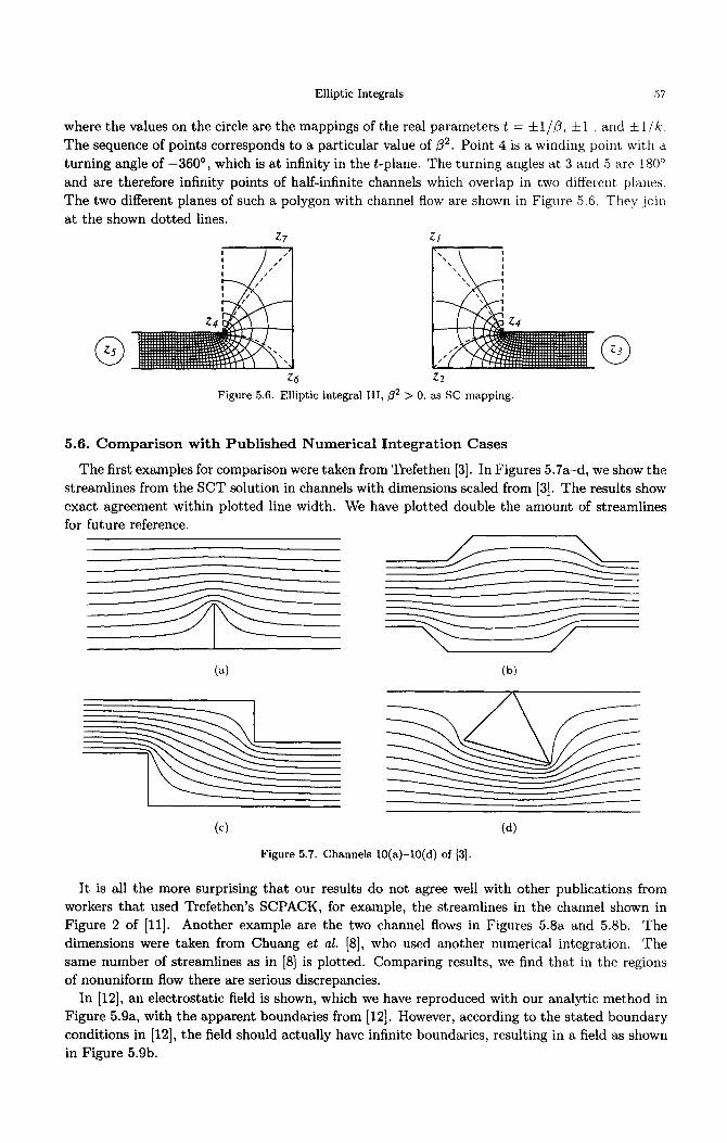
Elliptic Integrals 57
where the values on the circle are the mappings of the real parameters t = :t:1/~, ±1 , and ± l / k . The sequence of points corresponds to a particular value of ~2. Point 4 is a winding point with a turning angle of -360 °, which is at infinity in the t-plane. The turning angles at 3 and 5 are 180 ° and are therefore infinity points of half-infinite channels which overlap in two different planes. The two different planes of such a polygon with channel flow are shown in Figure 5.6. They join at the shown dotted lines.
Z7 Zl
', / "u !
Z6 Z2 Figure 5.6. Elliptic integral III, ~2 > 0, as SC mapping.
5.6. C o m p a r i s o n w i t h P u b l i s h e d N u m e r i c a l I n t e g r a t i o n Cases
The first examples for comparison were taken from Trefethen [3]. In Figures 5.7a-d, we show the streamlines from the SCT solution in channels with dimensions scaled from [3]. The results show exact agreement within plotted line width. We have plotted double the amount of streamlines for future reference.
(a) (b)
(c) (d)
Figure 5.7. Channels 10(a)-10(d) of [3].
It is all the more surprising that our results do not agree well with other publications from workers that used Trefethen's SCPACK, for example, the streamlines in the channel shown in Figure 2 of [11]. Another example are the two channel flows in Figures 5.8a and 5.8b. The dimensions were taken from Chuang et al. [8], who used another numerical integration. The same number of streamlines as in [8] is plotted. Comparing results, we find that in the regions of nonuniform flow there are serious discrepancies.
In [12], an electrostatic field is shown, which we have reproduced with our analytic method in Figure 5.9a, with the apparent boundaries from [12]. However, according to the stated boundary conditions in [12], the field should actually have infinite boundaries, resulting in a field as shown in Figure 5.9b.

58 W.C. HASSENPFLUG
, : ~
(a) (b)
Figure 5.8. Streamlines in channel[8, Figure 6].
I \ J I I k /
(a) (b)
Figure 5.9. Electrostatic field [12, Figure 3].
6 . R E V E R S I O N
6.1. I n t r o d u c t i o n
The terms inversion and reversion have often been used interchangeably, so that to avoid any confusion we define these terms as used in this section.
We use inversion as the term for the algebraic operation 1Ix on a variable x, in the current algebra, and we also use the exponent symbol x -1 for this operation. Inversion of a function f ( x ) is the inversion of the variable y = f ( x ) for all values of x, 1/y = l / f (x). This inversion is t ransformed in convolution algebra by the Taylor transform, see [20], into the operation
1 _ . - 1
We use reversion as the customary term for the operation of creating the function x = g(Y) out of the function y = f ( x ) , an operation that has no algebra and cannot be transformed into an equivalent convolution algebra operation. The corresponding operation in convolution algebra is a process rather than a single algebraic operation. If the customary symbol - 1 be used for this process, then we indicate it by the symbol used in [35], x = f [ - l l (y ) .

Elliptic Integrals 59
Particularly referring now to the SCT, the forward form is the nonhomogeneous linear differ- ential equation (4.1), with the scaling constant from equation (4.9),
dz(s) = c2 y [ ( s - sk) - ~ ~ f ( s k , s), (6.1)
d--~
which we will call the forward transformation, and the series solution z ( s ) , consisting of the set of expansions in the different convergence disks, is called the forward solution.
The revers ion of the Schwarz-Christ0ffel transformation is the homogeneous nonlinear differ- ential equation
1 ds(z)_~z = lc2 H ( s ( z ) - Sk)~k -- f ( s k , S(Z)) ' (6.2)
where the parameters sk remain the same. This corresponds to the form as posed by Trefethen [3] to be solved by an ODE solver " . . . to invert the Schwarz-Christoffel formula" in his terminology.
The iterative solution of s for a given value of z from the solution of equation (6.1) is not termed by us a reversion, but rather a reverse or inverse solut ion or computa t ion . As example, the inverse SCT by Costamagna [5] is merely the inverse computation of the forward SCT-solution.
In this section, we present certain solutions of the reverse transformation that can be found by convolution algebra.
6.2. P a r a m e t e r s
The parameters sk are as unknown in the reverse solution as in the forward SCT solution, and must be found by an iterative process if the problem is posed as a polygon in the z-plane. Therefore the known iteration method of the forward SCT may be used, which means the problem must be solved in the forward method first. Exceptions are the triangle, where the sk are arbitrary, and the rectangle, where the sk can be found by known explicit methods. It will be clear at the end of this section why we will not a t tempt to solve the parameter problem using the reverse SCT.
The reverse solution starts then with known parameters in equation (6.2) and its forward solution. From the same solution, the constants cx and c2 will be known.
6.3. T a y l o r Ser ies
Since the forward solution z ( s ) is assumed to be known, the point on the z-plane corresponding to the origin of the s-plane is known. Choosing a center z0 for the reverse expansion, the corresponding point so must be found iteratively from the forward solution. This is effectively the constant of integration, and the iteration complies with the fact that the initial value of a first-order differential equation must be found algebraically, see [20]. Using the transformed variables
u = s - so , v = z - z0 , uk = sk - so , (6 .3 )
equation (6.2) becomes
d u ( v ) ~ I - [ 1 (6 .4 ) ~V ---- (U(V) - Uk) ~k ==- f(uk, u(v))"
The solution of equation (6.4) in the regular region of the z-plane is the nonunit Taylor series
U ='UlV -~ U2 v2 -~- U 3 v 3 -~- • . .
- K " u , ( 6 .5 )

60 W . C . HASSENPFLUG
and the Taylor transform of equation (6.4) is
- ' (u - ) ° ' u = 1 - [ - uk 0 , ( 6 . 6 )
which is solved by pointer convolution numbers [20] in each Taylor convergence disk. The origin in the z-plane is arbitrary within the polygon, but the region of convergence is now
a disk in the z-plane within all singular points. This disk has no resemblance to the Taylor disks of the forward SCT. The singular points are all corners that do not have a turning angle of r/n. But there are also many points outside the polygon where z maps on s = co, and are therefore singular points of s(z), which limit the radius of the Taylor disk. We will demonstrate the Taylor solation in the following examples of special triangles and general rectangles.
6.4. T r i a n g l e s
There are three and only three special triangles where there are no singularities of the reverse function s(z) on the boundary. These are the three triangles shown in Figure 6.1. Let us now at tempt to obtain the reverse solution of the equilateral triangle.
Figure 6.1. Three special triangles.
Choosing symmetrical parameters in the s-plane, the values for the triangle are according to Table 6.1.
Table 6.1.
Corner a ~ z
1 120 ° 0 ° .8833216 + ~ 1.529958
2 120 ° 120 ° .8833216 + ~ 1.529958
3 120 ° 240 ° 1.766643 -I-~0
Since no parameter iteration is necessary, we choose So -~ 0 and z0 - 0, and see where the triangle is going to be relative to the origin in the z-plane. Choosing the constant c2 - 1, the differential equation to be solved is the convolution equation
The Taylor series is obtained as described above, and the result is shown in Figure 6.2a. The internal lines shown are mapped concentric circles in the s-plane, plotted by iterative solution of the Taylor series s(z), using convolution number length n = 20. The reflection of the center z0 about each of the sides is shown by a *. These are the points where s -~ co is mapped, therefore singularities of the function s(z). The distance of these points happen to be the same as the distance of the corners, which then determine the radius of convergence of the Taylor series. The numerical radius, using the factor 0.7, is shown by the dotted circle. The corners of the triangle are therefore not included in the central Taylor series, and can therefore not be computed directly from the Taylor series. But the midpoints of the sides are well within the numerical Taylor disk. Furthermore, from the differentials in equation (6.1) at the singular points, the orientation of each side of the triangle is known, depending on the branch of the fractional power. From this information we arrive indirectly, but with great accuracy, at the dimensions of the triangle.

Elliptic Integrals 61
Zl o ~ Zl
: : z3 : ~ !
22 t • Z2
(a) Central Taylor series s(z), n = 20. (b) Displaced Taylor series s(z - zo), r~ = 20.
%% z3
-
Z2 Z2 (c) Displaced Taylor series s(z - zo), n = 20. (d) Displaced Taylor series s(z - zo), n = 50.
Figure 6.2. Reverse Taylor series of equilateral triangle.
The dis tor ted shape of the mapped lines in Figure 6.2a verify clearly tha t there is no convergence
near the corners. Also, tha t the zeros of the first and second derivatives, s'(z) and s"(z), should bo th lie on the corners. But they are actual ly found at the points shown by a o, the zero of the
first derivative in the center and two zeros of the second derivative straddling the s y m m e t r y line. Therefore, while the dimensions of the triangle can be determined from the reverse Taylor series, the actual function s(z) near the corner must be determined with a second series.
As the next series we chose the center z0 = z3/2 for a Taylor disk. Wi th the usual t ransforma- tions, equat ion (6.7) becomes
~t = ("U - Ul-~O) "2/3 * (-u - lt2-~o) *2/3 * (-u - u3~o) .2/3 (6.8)
The apparen t numerical radius, determined again by the mapping of s = c~, includes now the
center of the tr iangle as well as the midpoints of the sides, so tha t we might still have one single
Taylor series for all points within the triangle, using the symmetry. The accuracy of the mapping seemed quite sat isfactory at n = 20, shown in Figure 6.2b. Yet we found the value of [s'(z)l = 1 at za, instead of zero. We can therefore not claim an analytic result, within machine accuracy, which is the purpose of the convolution number algebra. Even when we increased n, we could not get be t te r accuracy.
To show why this happens, we choose another point z0 = 0.75 z3 and use the previously de termined values of the corners zi, and the central series to determine so iteratively.
62 W.C. HASSENPFLUG
The solution is shown by the same mapping of circles in Figure 6.2c with n = 20, and Fig- ure 6.2d with n = 50. The reflected lines about the corner z3 are also plotted, representing the analytic continuation of s ( z ) outside the triangle. Instead of increasing the accuracy, the figures show clearly the the radius of convergence becomes smaller with increasing n. In fact, the results display a property similar as in asymptotic series, where the accuracy for a particular value of z increases first and then diverges with increasing n.
Inspection of Figure 6.2d reveals a convergence radius just beyond the corner za. On exam- ination we find the reason in the differential equation (6.8). In the computation of the term
( u - u3~0) .2/3, our numerical convolution algebra cannot distinguish between an exact power of 2/3 of an exact root, and a numerical approximation by digital computer. This particular factor is therefore divergent for all [ z - z0[ > [ z - z31, even if z3 is a zero of the function s ( z ) - s 3 , where theoretically a convergent series exists.
This is what causes the divergence shown so clearly in Figure 6.2d. Expressed differently, the method of computation of the convolution the factor is uns tab l e , and due to the recursion affects the whole convolution number u.
Tha t the radius is apparently a little larger than [z3 - z01 is due to the fact that the divergence is rather small near the theoretical Taylor expansion. The Taylor series including the corner z3 still exists, but we cannot find a stable method to determine it.
The reversion of the SCT for the three special triangles must therefore be carried out as for a general triangle, assuming singularities at the corners. A central Taylor series is obtained first, then the reverse solution at the corners is obtained by the reversion of the Frobenius series, as presented further below.
6.5. T h e R e c t a n g l e
The rectangle as boundary occurs quite frequently, either in mechanics because of the simple engineering shape, or in potential problems as region in the complex potential plane, e.g., [12]. The mapping of the rectangle is an exceptional problem for the SCT in as much only one un- known parameter has to be determined, allowing series expansions in a single variable, the known parameter. These have been extensively developed in connection with the elliptic integral of the first kind.
In the forward SCT, the parameter is the modulus k in the standard Jacobi form of equa- tion (3.1)
f0 t dt = F ( t , k) = V/(1 _ t2)( 1 _ k2t2 ) .
The corresponding rectangle has the dimensions 2K × K ~ in the C-plane, where K and K ' are the complete elliptic integral and the associated complete elliptic integrals of the first kind. Here we use the notation ~ instead of the classic notation u.
The customary reversion is the mapping of the rectangle on the upper half of the t-plane by the Jacobian elliptic function t =sn (~). Our reversion is slightly different because we map on a circle in the s-plane, which avoids the infinity which is present in sn (~). The differential equation to be solved for s ( z ) is
d s = l ( s _ s l ) l / 2 ( s _ s 2 ) l / 2 ( s _ s 3 ) l / Z ( s _ s4)1/2" (6.9) d z c2
If we choose four symmetric singular points on the circle, the relation between s and t of equa- tion (5.34) is
~ - v ~ t ~ 1 - s S = - - t----- - - - -
~ +v~ t ' v ~ l + s '
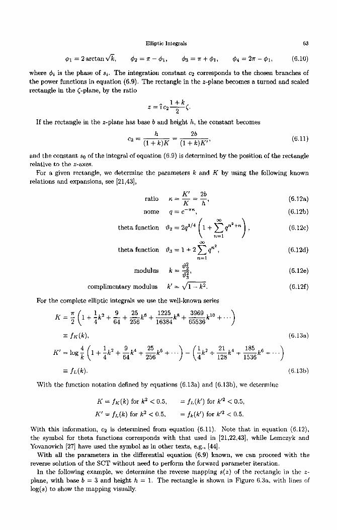
Elliptic Integrals 63
¢1 = 2 arctan x/k, ¢2 = 7 r - ¢1, ¢3=71"+¢1, ¢4 = 27r- ¢1, (6.10)
where ¢i is the phase of si. The integration constant c2 corresponds to the chosen branches of the power functions in equation (6.9). The rectangle in the z-plane becomes a turned and scaled rectangle in the (-plane, by the ratio
^ l + k . z = ~c2- -T~ .
If the rectangle in the z-plane has base b and height h, the constant becomes
h 2b ----- (6.11) c2 = (1 + k ) K (1 + k ) K "
and the constant so of the integral of equation (6.9) is determined by the position of the rectangle relative to the z-axes.
For a given rectangle, we determine the parameters k and K by using the following known relations and expansions, see [21,43],
K I 2b ratio a = K h ' (6.12a)
home q = e -~ ' , (6.12b)
theta function ~92 --- 2q 1/4 1 + q n2+n , (6.12c) n = l
oo
theta function ~3 1 + 2 E n2 -- q , (6.12d) n = l
modulus k = ~9.~ (6.12e) ~ '
complimentary modulus k' = v / 1 - k 2. (6.12f)
For the complete elliptic integrals we use the well-known series
7r ( 1 9 25k6 ~ 3969k10 ) K = ~ 1 + k 2 + ~ - ~ + ~ - ~ + k S + ~ + . . .
=- fK(k ) , (6.13a)
4 ( 1 25 6 ) ( 4 21 k4 185k6 " " ) K ' = log ~ 1 + k2 + 9 k 4 + 2--'~ k + . . . . k2 + 128 + 1536 +
=- fL(k) . (6.13b)
With the function notation defined by equations (6.13a) and (6.13b), we determine
K = fzv(k) for k 2 < 0.5, = fL(k ' ) for k '2 < 0.5,
K ' = fL(k) for k 2 < 0.5, = fk (k ' ) for k '2 < 0.5.
With this information, c2 is determined from equation (6.11). Note that in equation (6.12), the symbol for theta functions corresponds with that used in [21,22,43], while Lemczyk and Yovanovich [27] have used the symbol as in other texts, e.g., [44].
With all the parameters in the differential equation (6.9) known, we can proceed with the reverse solution of the SCT without need to perform the forward parameter iteration.
In the following example, we determine the reverse mapping s(z) of the rectangle in the z- plane, with base b = 3 and height h = 1. The rectangle is shown in Figure 6.3a, with lines of log(s) to show the mapping visually.

64 W . C . HASSENPFLUG
Z2 .~ •
! # I I !
',, /
Z3 "- " Z4
0
(a) Rectangle and lines log s in z-plane. (b) Constant x, y lines in s-plane.
Figure 6.3. Mapping of rectangle by reverse Taylor series.
The corresponding constants as determined from equations (6.10)-(6.12) are
k --- .3227981 x 10 -3,
~i --- 2.058597 °,
c2 -- .6364143.
Equation (6.9) is transformed to convolution numbers and solved by pointer numbers as an initial value problem. The initial value s(z -- 0) = 0 is evident from symmetry, therefore we start with a central Taylor series. The infinity points of s are mapped on the reflections of the origin about the sides, the nearest ones shown as sc~ in Figure 6.3a. These are the only singularities of s(z), which limit the numerical convergence radius as shown by the central dotted circle, using the empirical ratio of 0.7. To cover the remaining region on the right, we put another Taylor series at the center z0 halfway between the center and the right edge, which is just outside the inner Taylor disk. The second Taylor disk is again limited only by the two singularities shown, and passes just inside the corner points. In this case, we simply extend the numerical radius somewhat, using a larger length n for the expansions. For the central circle it becomes 0.75, and for the outer circle 0.721. Using the first Taylor series, the value So -= s(z = z0) is determined for the initial value of the second Taylor series, and the variables are transformed as in equation (6.3) to the new center.
The resulting two Taylor series are then used to cover the right half of the rectangle, and the
left by using symmetry. The function s(z) is displayed by means of constant x, y lines, enlarged near the boundary between Sl and s4, in Figure 6.3b.
ds To test the accuracy at the corners Zl and z4, we have computed the first derivative ~'7, which should be zero. Within machine accuracy, this is only achieved at n = 50. The second derivative, d28 ~rz, is not zero as for the equilateral triangle. We have computed its value by means of the Frobenius expansion of the forward SCT as -.0127354 + ~.3543014 at the corner Zl. This was verified by means of the reverse Frobenius series, as described later below, by the value of -.0127356 + 7.3543029, therefore accurate to ~, 6 digits. The values obtained from the reverse Taylor series are given in Table 6.2.
Therefore, the reverse Taylor series has converged well at the corners, contrary to the expec- tation that it would diverge there due to the destabilizing square root factor in the differential equation. Apparently that divergence is much less pronounced than was the case for the triangle. On the other hand, the large value of n required for good accuracy may just be due to this diver- gent contribution. We note also a slight unsymmetry in the values. This is probably due to the rather small angle difference ~b I - ~b4, typical of the large distortions in the SCT. Apparently this

Elliptic Integrals 65
Table 6.2.
d2s dz 2
n at Zl at z4
20 .0334748 -t- ~. 1950647 .0334896 - ~'. 1950764 30 -.0104412 + ~ .3630329 -.0104454 + ~ .3630360 40 -.0130508 + ~ .3540384 -.0130544 -I- ~ .3540325 50 -.0127189 -t- ~ .3543001 -.0127227 4- "~ .3543057 60 -.0127367 -t- ~" .3543040 -.0127329 -t- "~ .3542970 70 -.0127369 + ~ .3543036 -.0127324 + ~ .3542953 80 -.0127373 + ~ .3543042 -.0127316 4- ~ .3542948 90 -.0127376 + ~" .3543045 -.0127306 + "~ .3542936
100 -.0127376 -I-~ .3543050 -.0127300 4- ~ .3542927
tends to make the differential equation (6.9) ill-conditioned. Even when we took the precaut ion of making the four points sk exact ly symmetric , an unsymmet ry in the results remained.
Similarly, the reverse expansion for a rectangle of any ratio h/b cart be found, but the number
of series will depend on the ratio. Generally a single Taylor series is not possible. But for very' flat rectangles, the mapping on the circle becomes a problem as the angle 01 becomes rapidly
very small. While the reverse mapping function over the whole rectangle by a set of Taylor series has been
shown above, this me thod should be compared to other expansions. Such are obtained by posing
the equat ion
w = log s = log z + f(z),
and solving f(z) by the real boundary value problem
u(x, y) = log r + g(x, y),
where w = u + ~ v , log z = log r + ~ ¢ , f(z) = g(x,y) +~h(x,y). We would like to point out here t h a t the me thod of polynomials, or thogonalized on the boundary, does not work, because of the ill-conditioned matr ices t ha t occur, see [4]. We have solved a similar problem with a mere ratio of b/h = 2 on an Olivetti P r o g r a m m a with 22 digits. Using powers up to z m, we obta ined an
accuracy of 3 decimals. But an a t t empt do do the mapping problem on a modern P C with 7 digits, for the same ratio of b/h, failed completely, as it must when one a t t empts to represent a
diverging Taylor series by a polynomial. In some classic examples, see [45,46], not very elongated shapes were used, 10 to 12 decimals were employed, and accuracy of 3 decimals was obtained. Convergence with or thogonal polynomials is proved, see also [4], but the divergence problem lies in the expression of or thogonal polynomials by Taylor polynomials. For example, the computa t ion
of the values of Tchebychef polynomials Tn(z), expressed as Taylor polynomials, fails on a 7-digit compute r a lready at n > 20, near Izl = 1. But using the recursion formula for the values of Tn,
s tar t ing with To = 1, T1 = z, no such problem occurs even for n well over 100. A sat isfactory method is expansion in Fourier series, a method tha t is used for the classic
rectangle torsion problem, see [47], with the result of the form
27rn ~ 2~rn log s = log z +c + E ansin--~--z + EbnSinh---h--Z, (6.14)
n ~ l n ~ l
where the coefficients are t ranscendental numbers. This series converges over the whole rectangle; it differs from the Fourier series given in [21] for sn (4), which maps the rectangle on the upper half
on the t-plane, and which does not converge over the whole rectangle because of the s ingulari ty
¢ =~K'.
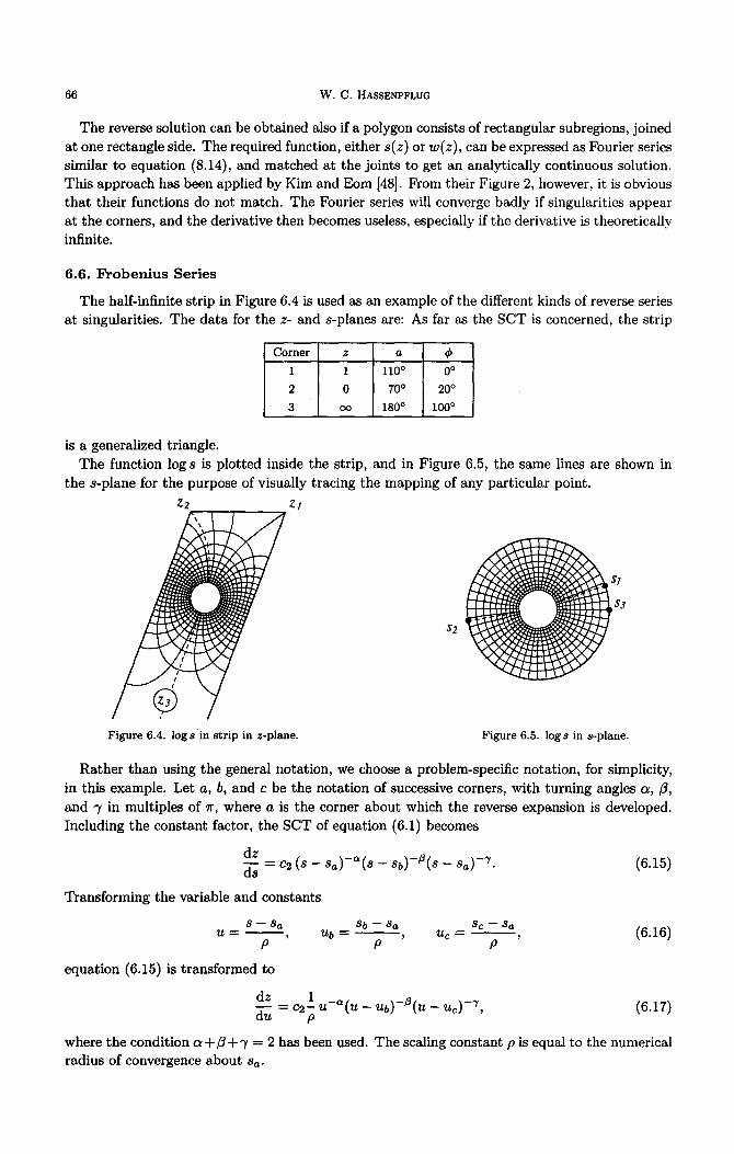
66 W . C . HASSENPFLUG
The reverse solution can be obtained also if a polygon consists of rectangular subregions, joined at one rectangle side. The required function, either s ( z ) or w ( z ) , can be expressed as Fourier series similar to equation (8.14), and matched at the joints to get an analytically continuous solution. This approach has been applied by Kim and Eom [48]. From their Figure 2, however, it is obvious that their functions do not match. The Fourier series will converge badly if singularities appear at the corners, and the derivative then becomes useless, especially if the derivative is theoretically infinite.
6.6. F r o b e n i u s Ser ies
The half-infinite strip in Figure 6.4 is used as an example of the different kinds of reverse series at singularities. The data for the z- and s-planes are: As far as the SCT is concerned, the strip
Corner z a ¢
i I I i 0 ° 0 °
2 0 70 ° 20 °
3 c~ 180 ° 100 °
is a generalized triangle. The function log s is plotted inside the strip, and in Figure 6.5, the same lines are shown in
the s-plane for the purpose of visually tracing the mapping of any particular point.
Z2 Zl
SI
$3
$2
Figure 6.4. log s i n s t r ip in z-plane. F igure 6.5. log s in s -plane.
Rather than using the general notation, we choose a problem-specific notation, for simplicity, in this example. Let a, b, and c be the notation of successive corners, with turning angles c~,/3, and 7 in multiples of ~r, where a is the corner about which the reverse expansion is developed. Including the constant factor, the SCT of equation (6.1) becomes
d z = c2 (s - s a ) - a ( s - Sb ) -a (S -- Sa) -'r. (6.15) ds
Transforming the variable and constants
S - - S a Sb--Sa 8c- -Sa U ~--- - - , ~Zb = ~ , Uc = - - , (6.16)
P P P
equation (6.15) is transformed to
dz 1 d'--u = c 2 - u - a (u - Ub ) -1 3 ( U - - Uc) -3', (6.17)
P
where the condition c~ +/3 + 3' -- 2 has been used. The scaling constant p is equal to the numerical radius of convergence about sa.

Elliptic Integrals 67
ORDINARY FROBENIUS SERIES. The forward Frobenius expansion about corners 1 and 2 has the form, according to equation (2.23), and including the integration constant cl and scaling constant c2,
z = cl + c2 (zo + u l - ~ ( z F o + ZFlU + . - . ) ) . ( 6 . 1 8 )
The point sa is mapped on the cornerpoint za such that
z~ = c l + c2zo, (6.19)
and we write equation (6.18) as
z - z a = u l _ a ( z f 0 + ZF1 i t + ' ' ' ) C2
= u ~ - ~ x ~ . z F . ( 6 . 2 0 )
We define the variable ( ~ 1/(1-~)
z - Za (6.21) \ c2 /
so that equation (6.20) is transformed to
--*l/(1--oc) V ~ u x U ' z F
[ 1/(l-a) U 2 ) = u x ~,Zfo + . . . u + . . . + . . . . (6.22)
Equation (6.22) is regular in both variables u and v and is therefore suitable for reversion. Obviously the leading part of the expansion in equation (6.18), Cl + c2(z0 + u l - ~ z f o ) , plays a major role, and we call it the principal part (PP).
Equation (6.21) defines a mapping from the z-plane on a v-plane, different for each corner. The mapping at corner 1 is shown in Figure 6.6a, and at corner 2 in Figure 6.6b. The mapped center of the s-plane is shown by a • inside the boundary. The reflection of this point by the straight line is shown by a • outside the boundary. As this latter point is the mapping of the reflection of s = 0 in the s-plane by the unit circle, which is oo, it is a singularity of the mapping function s ( v ) .
The mapped lines of the function log s show clearly that s ( v ) is a regular function within the boundaries, and is continued regularly in the reflection about the straight line boundary. The mapped corner 2 in Figure 6.6a, the mapped corner 1 in Figure 6.6b, and the mapped infinity point are singularities which limit the radius of convergence.
The numerical radius of convergence about each center is shown as determined in the v-plane. In Figure 6.6a, the radius is limited by the corner 2, but in Figure 6.6b, the infinity point is the one that limits the radius of convergence.
The purpose of equation (6.22) is only to arrive at suitably transformed variables. The reversion of a t runcated Taylor series is not exact, and needs as at least twice as many convolution variables as there are forward coefficients, see [20]. The actual reversion is carried out by solving the differential equation derived from equations (6.17) and (6.21),
~vv = (1 - v~)p (u - Ub)Z(u -- Uc) "y. (6.23)
In the reverse expansion, u is considered as function of v,
u = V- u; (6.24)
therefore the Taylor transform of equation (6.23) is
u = (1 - ~ ) p x • ~ - u b • u - ~ c , ( 6 . 2 5 )
which has to be solved for the convolution number u.

68 W . C . HASSENPFLUG
,,~oa
Y2
3oo
(a) Mapping around zz. (b) Mapping around z2.
Figure 6.6• log s in v-planes.
Equation (6.25) is free of the constants cl and c2, but they are still necessary for the relation between z and v in equation (6.21). Therefore, the forward SCT solution must be obtained first. Only in this example of a triangle, no iteration is required.
To solve equation (6.25), we define intermediate variables shown graphically in equation (6.26) below:
u --- ( 1 - ~ ) p x * ( ~ . . ~ . ~ ) ( ~ . ~ . 5 (6.26)
~'b r-c
Y ~b Uc U a
ql Y
From equation (6.22), it is clear that the reversed series in equation (6.24) is a nonunit,
u0 -- 0, (6.27)
so that equation (6.24) is in detail
u = U l V + u2v 2 + u 3 v 3 + . . . . (6.28)
From this property, it follows that the division U / 5 l in equation (6.26) is compatible. But it also implies tha t the shift of elements of convolution numbers on both sides of equation (6.26) is the same, on the left due to to the differentiation, on the right due to the division. We cannot employ directly the pointer number method, because the unknown element of u is the same in u and in p. Therefore we use the advance pointer method, see [20]. We define a function
- - ?
f = p - u (6.29)
which must be zero. To follow the theory clearly, a few algebraic steps are shown in detail. Let
(1 - a)p (u - U b ) ~ ( u - - We) ")' --~ ao '}- azu + a2u 2 + . . . . (6.30)

Elliptic Integrals 69
Substituting equation (6.28) and (6.30) into equation (6.23) produces the first elements
fo = aou~ - u l , (6.31a)
fx -- a lu~ +1 + aooLu~-au2 - 2u2, (6.31b)
1) f2 = a2u~ -t-2 Jr- alU2U~ -Jr" O~alU~U2 ~- ao 2 u~-2"tt22 -{'- a°c~u~-lu3 -- 3u3' (6.31c)
Consider equation (6.29) as implicit first-order differential equation -f ( u , u ' ) = 0. Equa-
tion (6.27) constitutes the necessary initial condition for a first-order differential equation. From the theory of [20, Section 13], we use the following results.
The first unknown element of u is solved from the element f0, with the solution
ux = alo/0-'~) (6.32)
The element fk does not contain elements ui>k+l. The element fk contains element uk+l linearly. Therefore we can express
a A - - . (6.33) fk = Yk(uo, Ul, u 2 , . . . , uk, 0) + duk+, Uk+l
From equation (6.31),
Oft: _ Opk (k + 1). (6.34) duk+l duk+l
From the theory in [20, Section 10], applied to equation (6.29), and using the solution equa- tion (6.31a),
Opk Opo . . . . c~. (6.35) duk+l dul
From equation (6.29) it is clear that f k on the r.h.s, of equation (6.33) can be replaced by Pk as defined in equation (6.26). The formula for the new element in the recursion routine is therefore
pk(uO, U l , . . . , Uk, O) uk+x = e~ - (k + 1) (6.36)
Equations (6.34)-(6.36) can be verified from equations (6.31a)-(6.31c). From equation (6.30) we find
a0 = (1 - o~)pu~(--Ub)~(--Uc) "~, (6.37)
and it can be verified numerically by using equations (6.20), (6.21), (6.30), and (6.23) tha t this is the same as
1 a 0 ~
zFO
Pointer convolution number algebra is used to determine the value of pk(u0, Ul . . . . . uk, 0) in a computation loop, using all the intermediate variables indicated in equation (6.26). Initial values are set for ux, Uao = u~, u ~ = (--Ub) ~, U¢0 = (--uc) 7, which sets the proper pointer to p = 0.
The advance number is a = 1, and the pointer in u is set to p + 1 at the beginning of each loop. This allows Pk to be computed without element Uk+x with the standard pointer routines. At the end of the loop, the element Pk is recalled, element Uk+l computed according to equation (6.36)

7'0 W . C . HASSENPFLUG
and inserted in u. The pointer of all dependent variables is now reset to p by subtracting 1 from the current value of p.
Care must be taken to choose the branch in the solution of the multivalued function in equa- tion (6.32) so that the result satisfies equation (6.31a) with the branch chosen there for u~.
*e Each exponent in the loop is computed by an functional routine. Generally for f = u , a
pointer routine is written to solve the differential equation
- - ! ! - - U ?
U
This routine is used as a subroutine for two reasons. First, it needs only to be written once for the three exponents in the main routine. But second, for each main loop the subroutine needs two loops, which would hold up the main routine if it were directly included.
The solution of equation (6.25) is carried out for cornerpoint 1, with the indices a, b, and c, and the values of the exponents (~, f~, and ~/referring to corners 1, 2, and 3, respectively. Since the constants cl, c2 and cornerpoints in all planes are assumed to be known from the forward solution, no matching is required.
The same equations apply to every corner which has a forward Frobenius series of the form of equation (6.18). Therefore, for cornerpoint 2, the indices a, b, and c, and the values of the exponents a, f~, and 7 refer to corners 2, 3, and 1, respectively.
FROBENIUS SERIES WITH LEADING LOGARITHMIC TERM. The forward Frobenius expansion from equation (6.23) about corner 3 has a logarithmic term according to equation (2.27),
Z = e I -~ c 2 (Z 0 -~ gOFIOgu + U___" Z F ) . (6.38)
Defining za as in equation (6.19), it follows that
z - z a l o g u + U zF -- = • ------ U . a . (6.39) C2gOF - - goF - -
Define now the variable
v = e (z-z ' ) / (c2g°F) , (6.40)
then
v = u x U . e ' ~ = _ . U . ~
= b l u + b 2 u 2 + . . . , (6.41)
which is a regular nonunit Taylor series. The reverse has therefore the same form as equa- tions (6.24) and (6.28). Equation (6.40) represents a mapping of the z-plane on a v-plane shown in Figure 6.7a. At the corners 1 and 2, u ( v ) has singularities. The central part is shown enlarged in Figure 6.7b, with the center s = 0 and its reflection on the straight line, representing s = or. This latter point is the singularity nearest to the origin and therefore determines the numerical radius of convergence, shown by the circle in Figure 6.7b.
Substitute now a, b, and c as indices and a , f~, and 7 as exponents at corners 3, 2, and 1, respectively, then from equation (6.17), and using the derivative of equation (6.40), we obtain the differential equation
du u " ~ -~ gOFp v (U -- ?.tb) (U -- U c ) ~/ ( 6 . 4 2 )

Elliptic Integrals 71
Y2 /
Y3
s ~
(a) Full v-plane. (b) Detail at v3.
Figure 6.7. logs in v-plane at z3.
and the Taylor transform
u = goFP × * u - ub * u - uc (6.43)
Equations (6.42) and (6.43) have the same form as equations (6.23) and (6.25), considering that - 1, and are therefore solved with the same advance pointer convolution number technique.
The constant a0 = 1, and ul - 1, so that equation (6.31a) is again satisfied.
REVERSION OF THE WHOLE POLYGON. The mapped regions of convergence about the corners in the z-plane are shown in Figure 6.8. The circles of the v-plane of corners 1 and 2 become circular
segments, and the circle of the v-plane of corner 3 becomes the straight line. There is yet an
uncovered region in the middle. This can be covered by a Taylor series in the z-plane. Choosing
the center at a point zk , the radius of convergence is limited in the z-plane by the reflection of s = 0 on both straight sides of the strip, so that the Taylor series is valid in the circle as shown
in Figure 6.8.
The forward transformation is
Z = Ca --b c 2 ( z 0 q- Zl u + Z2 u 2 + ' ' " ) . (6.44)
Let zk = Cl + C2Zo and transform again to the new variable
z - z k v = - - , (6.45)
C2
then the reverse expansion u = V . u is obtained from the differential equation
which is solved by normal pointer convolution number algebra. We can assume that the forward expansion around zk is not available because the point zk was chosen in the z-plane. Therefore, we find the corresponding point sk by iteration from the other available forward expansions, assuming that the whole unit disk in the s-plane was covered. With this information, we determine p as the numerical radius of convergence in the s-plane, to transform to the variable
8 -- 8 k u = (6.47)
P

72 W.C. HASSENPFLUG
Sc~ $1
Figure 6.8. Convergence regions in z-plane. Figure 6.9. z-lines mapped on s-plane.
In Figure 6.8 we have also shown a set of parallel straight lines to be used as visual display for the reverse mapping s(z) . These mapped lines are shown in the s-plane in Figure 6.9, using the solutions in the appropriate convergence disks, using convolution number length n = 20.
As a check, we also reversed the Taylor series of equation (6.44) directly according to the
method in [20, Section 20.2], using only the first five coefficients of ZF. The result was tha t the
first five coefficients of u by both methods agreed quite well, the first coefficient being the same. Note tha t the reversion of a t runcated Taylor series only approximates each coefficient, while the reverse solution form the differential equation gives a machine-exact result of each coefficient.
In this example, we have not considered the reflection of the center s = 0 on the curved
boundaries in the different v-planes, nor on the straight line 1-2 in the z-plane, because they are too far away to limit the radius of convergence. But with other geometries this may not be the case. Generally in every reverse problem all reflections may have to be considered.
FROBENIUS SERIES WITH FIRST TERM A LOGARITHMIC SERIES. The first term of the Frobenius series will be a logarithmic series when the turning angle at infinity is near lr, according to equation (2.26). Let the cornerpoint be zl and the turning angle al = 1 + 5, as shown in Figure 6.10a. The da ta for the SCT are:
Corner z a ¢ 1 oo 190 ° 0 ° 2 ~, ~ ~r 80 ° 120 °
3 0 90 ° 240 °
The slope of the wedge shape is 10 ° for this demonstration example. A logarithmic series will
actually be used only for much smaller angles, typically < i °. The mapped lines of concentric
circles in the s-plane are plotted to convey the mapping visually, the mapped position of the
center of the circle, s -- 0, is shown by a *.
The point 4 is chosen as Z4 = 1/5. The point z2 becomes then z2 = ~ (1/5)tan(6zr) ~ ~zr. The
SCT is
d..z_z = c2u_(1+6 ) (u - u2) -~(u - u3) -~, (6.48) du
and the integral has the form
z -- al log u + a2 log 2 u + a3 log 3 u + . . . + U . f ' . (6.49)
The P P is the logarithmic series, which maps the circle boundary through st into the two half- infinite straight lines at zx. Therefore, the transformation of the z-region near zl on the lower half v-plane is will be the reverse of the logarithmic series, which is a Taylor series in the variable

Elliptic Integrals 73
- . : = - . . . . . . . . . . . . . . . . . . . . . . . . . . . . . . . .
Z4 Z 3
(a) Narrow-angle polygon in the z-plane.
S~
I) 2
(b) Narrow-angle polygon mapped on the v-plane.
Figure 6.10.
log U, of which the reverse exists. The reverse is obtained directly by mapping of the region between the straight lines on the lower half of the v-plane by
v = (1 + ,Sz) -1 /~ , (6.50)
which has the derivative
dv _ vX+~" (0.51) dz
The straight lines shown in Figure 6.10a are mapped on straight lines in the v-plane by this transformation.
Equation (6.50) is ill-determined for small 5, and therefore expanded into the well-determined form, similar to equation (2.26),
v = e -z+O/2)~z2-(1/3)~2z%' '" (6.52)
which is valid for small 5 --* 0, and becomes equation (6.40) for ~ = 0. The mapped region in the v-plane is shown in Figure 6.10b. The reverse SCT for u(v ) is obtained from equation (6.48) and the analytical closed form derivative in equation (6.51),
du - 1 ( U ~ 1+'5 ~VV -- C-~ , v / (u - u2)~(u - u3) ~. (6.53)
This is of the same form as equation (6.25), and the solution is obtained by the same convolution number method in equations (6.26)-(6.36).
The radius of convergence of the reverse series is determined entirely by the singularities of u ( v )
in the v-plane. The smallest radius in this example is determined by s~ , which is the reflection of the mapping of point s = 0 in the v-axis. The corresponding convergence region is shown by the hatched side of the dotted line in the v-plane, and its mapped region in the z-plane, the hatched

74 W.C. HASSENPFLUG
side (to the right) of the left dotted line in Figure 6.10a. However, the numerical convergence
of the series in equation (6.52) is limited to z < 0.71z41 = 0.7/6, which affects the computation of v(z) in the reverse calculation. This region is shown by the hatched side (to the left) of the
right dotted line in the z-plane in Figure 6.10a. For small 6, this is a large number, which may
be sufficient for practical purposes in view of the transformed value of v, and u being close to 0.
But this is still an unsatisfactory situation in as much values of z as large as a computer allows,
should be able to be transformed. We conclude that this is not possible by an explicit method.
The only method we can find to transform values of z > 0.7/6 is to use the PP as a function z(v)
and then solve v(z) iteratively. In this example the expansion is given by
e - ~ l ° g v -- 1 Z - -
6
= - l o g v + 261og2v- ~621og3v + . . . , (6.54)
which has unlimited radius of convergence in the v-plane.
F R O B E N I U S SERIES W IT H S E C O N D T E R M L O G A R I T H M I C . A s example, we use the flow along a step in a wall shown in Figure 6.11a. The data for the z- and s-planes are:
Corner z a ¢
1 c¢ 360 ° 0 °
2 z 7r -90 ° 120 °
3 0 90 ° 240 °
P 4 . , P/ P3
(a) z-plane. (b) v-plane.
F igure 6.11. M app i ng of s tep in wall.
The corner at infinity is the point zl. The SCT according to equation (6.1) becomes for this c a s e
d_~z = c2u_2( u _ u 2 ) X / 2 ( u _ u3)_l/~ (6.55) du
with the usual transformed variable u according to equation (6.3). The Probenius expansion around point 1 is, according to equation (2.27),
Z ~- C. 1 "4- C2 (7-,0 "[- ZFO u - 1 "[- ZF1 log u + ZF2U "[- ZF3 u2 "4-'" ") . (6.56)
The PP of the series in equation (6.56) is ZFOU - 1 + zF1 log u, which is the part that transforms the regular circle boundary through point sl into the two half-infinite straight lines in the z-plane,

Elliptic Integrals 75
where the logarithmic term corresponds to the parallel offset of the straight lines. Unlike the
ordinary case, we do not have a simple explicit reversion of the PP to transform the boundary
near point zl of the z-plane into a straight line of the v-plane similar to Figure 6.7a. The best we can do is to use the PP as implicit function to transform the z-plane into the v-plane by
1 z = - - log v. (6.57)
v
The mapped flow in the v-plane is shown in Figure 6.11b. The corners z2 and z3 are mapped conformally into corners v2 and v3, but the transformation has a singularity at a point z4, z = - 1 + ~ 7r, causing the corner at v4, v = - 1 .
Using equations (6.55) and (6.57), the reverse SCT becomes
d--~ = -c2 (1 + v)
Near v = 0 the reverse function u(v) is regular and can be expanded in a nonunit Taylor series as in equation (6.5). The Taylor transform of equation (6.58) is then
u , * (1 + ~1) (6.59)
*2 The convolution division inside the term (u / 51 ) is again compatible. The division by 1 + ~1 causes the limit Ivl < 1 of the Taylor series, corresponding to the contraformal point v4. The mapping of the center of the circle, s = 0, is shown by a • in the z-plane in Figure 6.11a and in the s-plane in Figure 6.1lb. The reflection of this point in the real v-axis, marked soo, is the singularity of the function u(v) where s = (x~ and therefore u = co. Therefore, the numerical radius of convergence in the v-plane is determined by the lesser of distances of - 1 and soo in the v-plane, from which the radius of the Taylor disk is determined as indicated by the dotted line in Figure 6.1lb. The corresponding region that is covered in the z-plane is shown in Figure 6.11a as the hatched side of the dotted line.
The convolution number solution of equation (6.59) proceeds as in the previous example, by the sequence of equations (6.26)-(6.36).
The result is tha t the complete reversion s(z) includes the iterative solution of v(z) from equation (6.57), and therefore the purpose of reversion, to obtain an explicit function s(z), is in this case only partially achieved.
CONCLUSION. The reverse of a Frobenius series is an ordinary Taylor series in a t ransformed variable. The Principal Part , PP, of the Frobenius series is the te rm tha t t ransforms the regular circle boundary through the cornerpoint point sa into the two straight lines from the corner za in the z-plane. The reverse of the PP transforms this corner in the z-plane into a straight line in the v-plane, which has then a suitable region around the transformed point va for the reverse Taylor series. The PP can be reversed explicitly in the ordinary case, or iteratively in cases containing the logarithm or a logarithmic series after the first term.
The reverse of a Frobenius series is not a Frobenius series. If there was only one te rm in the SCT, the forward and the reverse would be of the same form. But the forward expression has a "tail" after the first term, which makes the forward and reverse forms different.
6.7. L a u r e n t Ser i e s
For the reverse series solution, the Laurent expansion is just as important as in the forward series, i.e., it would need in some cases too many small Taylor disks to cover the region in the z-plane.

76 W.C. HASSENPFLUG
An example is shown in Figure 6.12a with the following data:
Corner z a ¢
1 - . 1 3 3 8 6 4 5 - ~ . 3 6 8 8 4 6 2 5 5 ° 1 . 6 6 7 6 0 7 °
2 - . 6 3 9 5 8 3 8 - l' 1 . 7 6 2 2 9 0 100 ° 1 6 5 . 0 7 5 5 °
3 . 7 2 5 8 5 5 2 - ~ 2 . 0 0 0 0 0 0 120 ° 1 9 4 . 9 2 4 6 °
4 . 1 1 0 0 9 2 4 - l" . 3 0 3 3 4 5 4 85 ° 3 5 8 . 3 3 2 4 °
Two straight line segments of the polygon are to be mapped on a single straight line in the
v-plane, shown in Figure 6.12b. The transformation v(z) may be explicit or implicit by the same method as described for the reverse of Frobenius series before. In this case, the straight lines meet in a point z0 = 0, and the transformation is explicit, v = (.720 - ~ . 6 9 4 ) z 4"5. The mapped concentric circles of the s-plane are shown in Figure 6.12a to visualize the mapping.
Z0
I t I %%
Z, I '~Z4
Z3 (a) Q u a d r i l a t e r a l in z - p l a n e .
//,, 'f, 'P'~zt#~ z
(b) L a u r e n t a n n u l u s in v - p l a n e . (c) I n n e r L a u r e n t c i r c l e in v - p l a n e .
F i g u r e 6 .12 . Q u a d r i l a t e r a l for r e v e r s e L a u r e n t ser ies .
The par t of the v-plane that includes the s ~ point is shown in Figure 6.12b, with the Laurent outer radius limited by the point s~, which is the reflection of the center s = 0, as shown. Figure 6.12c is enlarged by a factor of 50 to show the how the inner Laurent radius is limited by the included corners at vl and v4. The full annulus of the v-plane is shown as the sector in the z-plane Figure 6.12a.
The function s(v) is analytic in the annulus, and therefore a regular Laurent series of the reverse s(v) exists.

Elliptic Integrals 77
However, we have no Laurent convolution number algebra available to solve the differential equation of the reverse SCT. The only method we can suggest is to calculate the values of z(v) at a number of points on the two circles, iteratively from the forward solution, and then to calculate the Lanrent coefficients by a discrete Fourier analysis on both circles. A large number of points must be used to minimize aliasing.
6.8. C o n c l u s i o n
We have described how the reverse SCT of any polygon can be solved by Taylor series analyti- cally and Laurent series numerically. As in the forward transformation, a separate series for each corner is required, but a transformation to a new variable v(z) must be made first. The reverse series at the corners are regular series of the transformed variable, not Frobenius series as in the forward solution. Additional Taylor series may be necessary to cover the complete polygon. The reverse of the rectangle can be covered by Taylor series only.
Except for the rectangle, the reverse solution is much more complicated than the forward for several reasons. First, the forward solution must in any case be obtained first to get the parameters. Second, the distribution of singular points that limit the convergence disks is more complicated. Third, at the corners a transformation of variable v(z) must be made, for which in some cases we could not find an explicit form. Finally, a differential equation must be solved, which at the corners require a special pointer method. For the Laurent series only a discrete numerical solution could be found.
If one would a t tempt the solution of the parameter problem by the inverse SCT, the additional problem is tha t the position of the singularity s(v) = oo is not known, and therefore convergence disks are not known at the start of the problem. The solution of the forward SCT to find the parameters is therefore much simpler even if the reverse solution is actually sought.
The only remaining advantage of any reverse solution is that points s(z) can be computed explicitly faster than from iteration of z(s) by a factor of between 2 and 6. In any particular application, this advantage will have to be warranted compared to the large programming effort.
7. E X T E R N A L P O L Y G O N
7.1. G e n e r a l S o l u t i o n
The SCT according to equations (4.1) and (4.3) maps the interior of the unit disk in the s- plane on the exterior region of a polygon, which we call the external polygon. It seems natural to rather map the exterior of a unit disk on the exterior of the polygon, and substitute the negative turning angles in Figure 5.1d by positive turning angles/~ = - a i . With the transformation
1 = - (7.1)
8
we obtain a formula for the exterior mapping
1~ ~l 1 ) ~2 1 ~"
The far exterior region is then mapped in a natural way by a half infinite Laurent series
¢I C2 z=(+T (7.3)
of which the simplest example is the Joukowski transformation. If one deals only with exterior polygons, then the mapping of the exterior on the exterior according to the SCT of equation (7.2) is appropriate. Yet the Frobenius series about the singularities are still of the Taylor form, as well as any series of the filling disks. The Frobenius disks of the exterior SCT are not the same

78 W . C . HASSENPFLUG
as the Frobenius disks of the interior SCT, because although circles transform to circles by the inversion of equation (7.1), their centers do not transform to centers.
For the sake of uniformity of this treatise, we use the mapping of the interior disk in the s-plane also for the exterior polygon, and negative exterior angles as in Figure 5.1b. We also keep in mind that an exterior region is topologically still an interior region, with the result that the direction of the boundary of the exterior polygon is clockwise.
It has often been assumed that the center of the disk, s = 0, should be transformed to the infinity point in the z-plane, z = cx), as in equation (4.1); see [34,35]. But this often leads to an undesirable distribution of points on the circle. Therefore, a more general form of equation (4.1)
will be used, where the interior point s = b is mapped on z = oo,
Equation (7.4) is obtained by a M6bius transformation of equation (4.1), and this form is invariant under M6bius transformation. Particularly for the external polygon, n = -1 , equation (7.4)
becomes
z= f
- J g(s) ds, (7.6)
which transforms the point b inside the s-disk to z = co. Equations (7.4) and (7.5) are cast in
a form that is suitable to include the case b = 0. The natural form of the mapping as z ~ oc is then done indirectly by a complex potential w according to the case of the problem, as in the two examples in this section. The form of equation (7.5) corresponds to the form given for the mapping of the half-plane on the exterior region in [28,35].
To obtain a mapping which is continuous at z = ~ , the residue of the expansion of g(s) in
equation (7.6) about b must be zero, see [28], which is found to be
sai - b + 21 -- b 2 - r(b) = 0, (7.7)
where 52 = Ibl 2 = b b. For any distribution of points on the circle, sai = e ¢', which we call a
constellation, let us denote the array of angles ¢i, arranged as ¢i < ¢i+t, by a vector ~ n . For
any chosen constellation ~ n of an exterior problem, we must solve equation (7.7) for b. The condition equation (7.7), for the central form as in equation (4.1), is given by [28], but we could find no proof of the following hypothesis.
For every given constellation of-¢ n, n > 2, and the condition Y].ai = -2 , there is one and
only one solution s = b of r(s) = 0 in the disk, Ibl < 1.
The problem is that equation (7.7) is not an analytical function of the complex variable b, and therefore the Shur-Cohn algorithm [35] cannot be applied directly.
The solution of equation (7.7) is done by the Newton-Raphson method, but is not always easy because of large variations of It(s)[ for extreme polygons.
Since the inner point b is mapped on z = oo, it is also clear that an exterior polygon can have no positive corners (as > 0) at infinity. Therefore all polygons with positive infinity corners are interior polygons. In view of this fact, it is interesting to note that the only external S C T with 2 corners is the Joukowski transformation. Negative infinity corners may appear, but these would be sheets that run through the enclosed interior region to overlap with the continuous exterior region.

Elliptic Integrals 79
There are now altogether n + 2 singular points, of which n are on the circle, one is the internal
point b, and one is its external reflection at s = 1 / b . On the boundary we need n Frobenius expansions, and another one Frobenius expansion in the interior of the s-disk. The external
Frobenius series at 1 /b is never required, but the point has to be considered in limiting the radii of the other disks. Compared to the internal polygon, we have the additional factors, transforming to the scaled variable u = ( s - b ) / p , where p is taken as the radius of the disk,
(~ ~ ) - ~ ( 1 - ~ ) -~ - _ - = U * g n l * g n 2 ( 7 . 8 )
in the Taylor series of g ( s ) in equation (7.6). The one additional Frobenius series at point b is
(~-~) ~ (~- ~ ~)-~ ii~-~o.~-o, _ - u ~ _~,~ ~ Due to the integral power, there is no discontinuity branchline out of this disk, subject to equa- tion (7.7).
To demonstra te the effect of the eccentric point b, an initial uniform constellation -~n of a typical 10-cornered external polygon is shown in Figure 7.1a. The internal Frobenius disk at
and its external counterpart at 1 / b are shown. If the mapping of s = 0 on z = co is used,
the balanced constellation with b is as shown in Figure 7.lb. Clearly this is an unfavorable distribution of points on the circle.
lJ?,
(a) Balanced g # 0. (b) Balanced g = 0.
Figure 7.1. Boundary disks for the same external polygon.
The programming of the external polygon solution follows the same sequence as the internal solution. The tables of regions contain information of all n + 2 disks. The last row of the table is not complete because the expansion of the external series is not used.
7.2. S o u r c e a n d U n i f o r m F l o w
The complex potential w of the flow of a source or vortex in the z-plane is mapped on the s-plane by
~_-~,o~ ( ~ - ~ ) - ~lo~ (~ s - 1 ) , ~0~ m
h -- - - = real for a source, 21r - ~ F
h = - - = imaginary for a vortex, 2zr
of which an example is shown in Figure 7.2a.
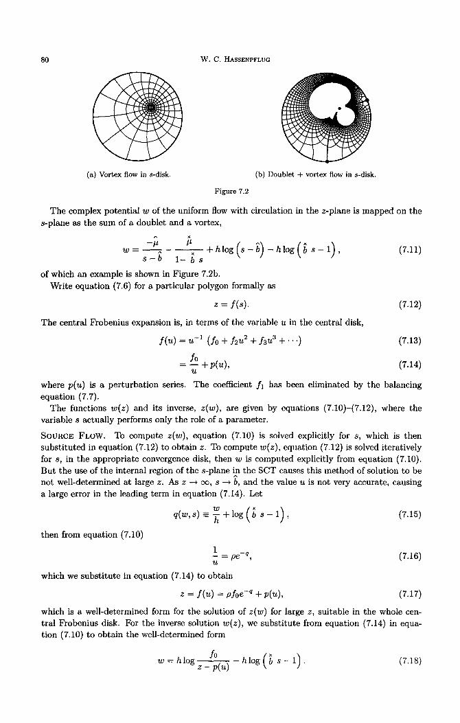
80 W . C . HASSENPFLUG
(a) Vor tex flow in s-disk. (b) Double t + vor tex flow in s-disk.
F igure 7.2
The complex potential w of the uniform flow with circulation in the z-plane is mapped on the s-plane as the sum of a doublet and a vortex,
^
s-b 1 - b s
of which an example is shown in Figure 7.2b. Write equation (7.6) for a particular polygon formally as
z = f ( s ) . (7.12) The central Frobenius expansion is, in terms of the variable u in the central disk,
f ( u ) = U -1 (fo "1- f2u 2 "-t- f3 u3 "-I-'" ") (7.13)
f o = - - + p(u) , (7.14)
U
where p(u) is a perturbation series. The coefficient f l has been eliminated by the balancing equation (7.7).
The functions w(z ) and its inverse, z (w) , are given by equations (7.10)-(7.12), where the variable s actually performs only the role of a parameter.
SOURCE FLOW. To compute z (w) , equation (7.10) is solved explicitly for s, which is then substi tuted in equation (7.12) to obtain z. To compute w(z ) , equation (7.12) is solved iteratively for s, in the appropriate convergence disk, then w is computed explicitly from equation (7.10). But the use of the internal region of the s-plane in the SCT causes this method of solution to be not well-determined at large z. As z --* oc, s --* b, and the value u is not very accurate, causing a large error in the leading term in equation (7.14). Let
) q(w, s) =-- -~ + log s - 1 , (7.15)
then from equation (7.10)
1 -- = pe -q, (7.16) U
which we substitute in equation (7.14) to obtain
z = f ( u ) = pfoe -q + p ( u ) , (7.17)
which is a well-determined form for the solution of z (w) for large z, suitable in the whole cen- tral Frobenius disk. For the inverse solution w(z ) , we substitute from equation (7.14) in equa- tion (7.10) to obtain the well-determined form
w = hlog f0 - h l o g ( b s - 1 ) . (7.18) z - p ( u )

Elliptic Integrals 81
The source or vortex potential of an external polygon is shown in Figure 7.3a. This could be an electrostatic or magnetic field, or a coordinate grid for another problem. The convergence disks are shown in Figure 7.3b. Probenius disks are shown in thick lines and Taylor disks in thin lines; there is no Laurent disk in this example. The external Frobenius disk is too far away to be shown.
(a) Source flow of external polygon. (b) Convergence disks for (a).
Figure 7.3.
UNIFORM FLOW WITH CIRCULATION. For the computation of z(w), we must solve equa- tion (7.11) iteratively for s, which is the normal procedure in flow inside or outside a circle. Then s is substituted in equation (7.12). The inverse solution z(w) starts again with the iterative solution of s from equation (7.12), then w is computed explicitly from equation (7.11). For large z,
we substitute 1/(s - b) = 1/pu from the leading term in equation (7.11) into equation (7.14) to obtain
z - -~ w + - - hlog(pu)+hlog(b s - 1 ) +p(u), (7.19) # 1 - b s
which is a well-determined form for the problem z(w) in the central Frobenius disk. The term log(pu) is small compared to w.
For the inverse solution w(z), we substitute the leading term in equation (7.11) by the leading term of equation (7.14) to obtain the well-determined form
^ z - p ( u ) ~ + h l o g ( pfo "~ ( s - l ) (7.20) pro z-p(u)) - hlog. , w : - ] £
where s is again first found iteratively from equation (7.12). From equations (7.18) and (7.20), it is clear that w and z are properly matched at z ~ oc.
The fact tha t the point s = 0 is mapped on some finite point in the z-plane does not matter at all. What counts is that the singularity of w(s) is situated at the point s = ~) which is mapped on z = oo.
The flow over an external polygon is shown in Figures 7.4a and 7.4b. The circulation and direction of uniform flow has been adjusted in equation (7.11) by selecting particular corners

82 W.C. HASSENPFLUG
on the circle as leading and trailing stagnation points. The figures also show that overlapping regions may occur in external polygons. There may also be winding points, which are points with turning angle - a > r. The discontinuity of the potential is not visible in the streamlines, and such a potential is only possible in pseudo-potential problems, like irrotational flow and magnetic fields.
(a) Symmetric. (b) Unsymmetri¢.
Figure 7.4. Uniform flow with circulation over external polygon.
8. P E R I O D I C P O L Y G O N
8.1. I n t roduc t i on
The periodic polygon has been computed successfully by numerical integration by Floryan [38]. Using the upper half of the complex t-plane, with the infinite straight line as boundary, he extends the SCT formula to the infinite number of corners of the periodic polygon. The method is based on his discovery that only a finite number m of corners have to be used for the actual computation. Therefore Floryan [38] computes a polygon with a number m of similar polygon sides, and two straight half-infinite sides. This is the same as using the well-known fact that the details of a far enough part of the boundary has an asymptotically decreasing influence on the near solution. In fact, theoretical infinities are such an approximation in reverse of any real polygon. In our method of using the unit disk as premapping plane, such an approach is not feasible because decreasingly small Frobenius disks will be crowded infinitesimally at the infinity point.
The disadvantage of the method of [38], albeit small in numerical integration methods, is that rn times as many product terms have to be computed than actual different sides of the polygon.
8.2. Per iodic Mapping
The formula given in equations (4.1) and (4.7), and derived in Appendix B, is an explicit closed exact formula, with only the required number of terms and singularities, which is well adapted to our method requiring a finite number of convergence disks. A MSbius transformation of equation (4.1) results in
-/g(s) ds. (8.2)
The form of equation (8.1) is invariant under bilinear transformation, and allows favourable adjustment of the distribution of corners on the circle.
The central Frobenius series around point b is
z=golog(s-b) +U__'ZF. (8.3)

Elliptic Integrals 83
The logarithmic term is the one providing the multivalued periodical values of the the SC in- tegral z(s). The function z(s) is not a continuous function in the s-disc as was the case with the previous polygons. The s-disc, considered as reverse function s(z), consists therefore of in-
finitely many sheets of a Riemann plane. The singularity at b causes an additional limit of the convergence disks. An example of typical convergence disks is shown in Figure 8.1a~ with the discontinuity branch from b. The mapping of the boundary is shown in Figure 8.1b, yet without any particular scaling constant c2, where the resulting complex period p is indicated.
\
\ " \ ,
( "'!, " ' \ " \ , \
\ \
(a) Periodic regions for 3 corners. (b) Periodic boundary with 3 corners.
Figure 8.1.
The Frobenius, and additional Laurent and Taylor, expansions are obtained by convolution algebra as in the previous sections. Matching of the series is done such that the centers of the convergence disks are in one consistent sheet of the Riemann plane. The overlapping of some of the disks occurs in different sheets. Here only the central expansion needs special attention.
There is no particular constraint equation for the choice of t h e parameter b as was the case in the external polygon. But the complex period p is a function of b. The factor in the logarithmic term is go of the central Frobenius series, which is from a theorem in convolution algebra [20] directly obtained from the function g(s) of equation (8.2)
and the complex period is
= 2 ~ g 0 . (8.5)
The periodic polygon can then be lined up as required with the z-axes, as shown in Figure 8.2a, with a particular possible flow field w(z). The complex potential is shown in the s-plane in Figure 8.2b,
(log (s w= 2 7 Therefore, near infinity of the z-plane we obtain the perturbation form
log W ~ - - X - - - . _ _
P
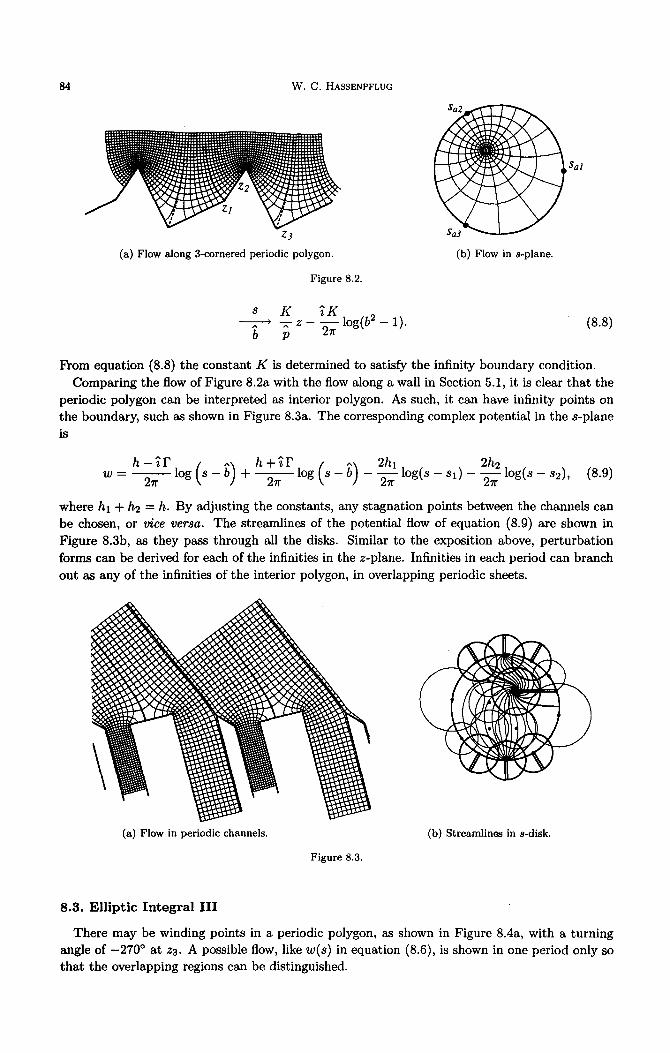
84 W . C . HASSENPFLUG
$a2
Sal
Z3 Sa3
(a) Flow along 3-cornered periodic polygon. (b) Flow in s-plane.
Figure 8.2.
s K ~K , ~ - z - ~ - log(b z - 1) . ( 8 . 8 )
p
From equation (8.8) the constant K is determined to satisfy the infinity boundary condition. Comparing the flow of Figure 8.2a with the flow along a wall in Section 5.1, it is clear that the
periodic polygon can be interpreted as interior polygon. As such, it can have infinity points on the boundary, such as shown in Figure 8.3a. The corresponding complex potential in the s-plane is
w = 2 ~ log - b) + ~ log 2hi log(s - 8 1 ) - 2h2 log(s - s 2 ) , (8.9)
where hi + h2 -- h. By adjusting the constants, any stagnation points between the channels can be chosen, or vice versa. The streamlines of the potential flow of equation (8.9) are shown in Figure 8.3b, as they pass through all the disks. Similar to the exposition above, perturbation forms can be derived for each of the infinities in the z-plane. Infinities in each period can branch out as any of the infinities of the interior polygon, in overlapping periodic sheets.
)
(a) Flow in periodic channels. (b) Streamlines in s-disk.
Figure 8.3.
8 . 3 . E l l i p t i c I n t e g r a l I I I
There may be winding points in a periodic polygon, as shown in Figure 8.4a, with a turning angle of -270 ° at zz. A possible flow, like w(s) in equation (8.6), is shown in one period only so that the overlapping regions can be distinguished.

Elliptic Integrals 85
® ®
Z ~ 3 z 4 ~ z2
Z5 Zl Z5 Zl
(a) Periodic polygon with winding point. (b) Elliptic integral III,/?2 < 0.
Figure 8.4.
W h e n mapp ing the real axis of the t -plane on the un i t circle in the s-plane by the bi l inear
t ransformation
l + ~ t ^ 1 - s s = ~ t = ~ - - , (8.10)
1 - 1 t ' 1 + s
the elliptic integral of the third kind
dt (8.11) z = (1 - 1~2t2) ~/(1 - tz)(1 - k2t ~)
is t ransformed to
5 5 f Z C/(S b)-l(1 -- 58) -1 -- H(S 8 = - __ - a i ) - " ' ds, ~ c ~ i = 0. (8.12)
J i=1 i=1
For real/~2 < 0, called circular cases [21],
{ c~ = (8.13) b - 1 + - 2 , i = 5 ,
which in this form is seen to be a mapping of the s-circle on a 5-cornered periodic polygon, with the two singular points b and 1/b not on the circle. The mapping is like a further distortion of the mapping of Figure 8.4a, with 4 corners of 90 °, and where the winding angle is increased to - 3 6 0 °. The winding corner is not visible in the real form of equation (8.11), because it happens at infinity on the real axis, which is mapped on the finite point s = - 1 .
The same flow from equation (8.6), Figure 8.2b, is shown mapped into one period in Figure 8.4b, with two adjacent overlapping rectangles. The adjacent periods are joined at the vertical potential line above the rectangle.
8.4. N o n p e r i o d i c F l o w
The s t ream or potential function in the examples above is continuous in the s-disk, resulting in periodic flow in the z-plane. If for any reason nonperiodic flow exists, then the mapping of the periodic polygon on the upper half of the t-plane is required, with all periods of the z- plane mapped on a continuous sequence of rectangular half-infinite strips of the t-plane. This is accomplished by mapping all sheets of the Riemann plane in the s-disk on the t-plane by the t ransformation
l -~ e2r~ t t = log s, s , (8.14) 2rr7

8 6 W . C . HASSENPFLUG
where the point b is shifted to 0 by a bilinear mapping first. The central Frobenius series then becomes
,, ^ Z f z k s k Z = C2go log S +
= t + Z f z k e ~rk;t (8.15)
S ~t
0
using equation (8.5), and choosing the constant c2 = 1 /p . Equation (8.15) constitutes a uniform map plus a Fourier series, valid for ~(t) > ( - log p)/2~r. On the boundary the different Frobenius, Laurent, or Taylor series apply.
It is therefore easy, once the periodic mapping solution is available, to map any flow in the upper half of the t-plane on the periodic polygon in the z-plane. An example is shown in Figure 8.5.
I I I I I I I I I I
Figure 8.5. Nonperiodic flow in periodic mapping.
9. C Y C L I C P O L Y G O N
The purpose of the SCT for cyclic polygon is a time saver, considering that all polygons can be mapped with the three basic forms of internal, periodic, and external forms.
Let the original disk be in the C-plane, and consider the regular SCT formula of equation (4.1) for a polygon with m cycles and n corners in each cycle. If the points of each cycle are spaced in equal sectors of the circumference of the ~-disk, then the SCT formula of equation (4.1) becomes the well-known SCT formula for the cyclic polygon, see [34,35],
n
z = f c J H ( ¢ m - ¢~)-a~ de, (9.1) i----1
where j -- 0 for the internal and j = - 2 for the external polygon. The SCT of the cyclic polygon with m cycles is obtained from the symmetric form of equation (9.1) to a new s-disk by the transformation, see [28],
s = ;m, (9.2)
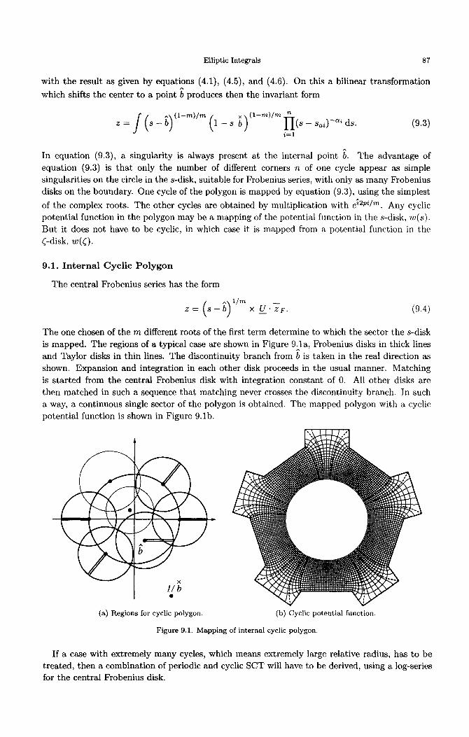
Elliptic Integrals 87
with the result as given by equations (4.1), (4.5), and (4.6). On this a bilinear transformation
which shifts the center to a point b produces then the invariant form
z = - - s b ) i i ( s - s o i ) - o , d s ( 9 . 3 ) i = l
In equation (9.3), a singularity is always present at the internal point b. The advantage of equation (9.3) is that only the number of different corners n of one cycle appear as simple singularities on the circle in the s-disk, suitable for Frobenius series, with only as many Frobenius disks on the boundary. One cycle of the polygon is mapped by equation (9.3), using the simplest
of the complex roots. The other cycles are obtained by multiplication with e ~2pilm. Any cyclic potential function in the polygon may be a mapping of the potential function in the s-disk, w ( s ) .
But it does not have to be cyclic, in which case it is mapped from a potential function in the C-disk, w(;) .
9.1. I n t e r n a l Cyc l i c P o l y g o n
The central Frobenius series has the form
z = s - x U . z F . (9.4)
The one chosen of the m different roots of the first term determine to which the sector the s-disk is mapped. The regions of a typical case are shown in Figure 9.1a, Frobenius disks in thick lines and Taylor disks in thin lines. The discontinuity branch from b is taken in the real direction as shown. Expansion and integration in each other disk proceeds in the usual manner. Matching is s tarted from the central Frobenius disk with integration constant of 0. All other disks are then matched in such a sequence that matching never crosses the discontinuity branch. In such a way, a continuous single sector of the polygon is obtained. The mapped polygon with a cyclic potential function is shown in Figure 9.lb.
(a) Regions for cyclic polygon. (b) Cyclic potential function.
Figure 9.1. Mapping of internal cyclic polygon.
If a case with extremely many cycles, which means extremely large relative radius, has to be treated, then a combination of periodic and cyclic SCT will have to be derived, using a log-series for the central Frobenius disk.

88 W.C. HASSENPFLUG
{}.2. E x t e r n a l Cycl ic P o l y g o n
The central Frobenius series has the same form of equation (9.4), except that the number of cycles is counted with a negative number m. In contrast to the single external polygon, no logarithmic terms appear in the central Frobenius series for any finite m, and therefore no balancing of the position b is required. Interestingly, if we, for example, treated an external polygon with m-cycles as simple external polygon with - m x n corners, then balancing would be required.
The only difference in the iteration computer program is that allowance must be made for negative m where this is used as counter.
An external cyclic polygon with the same geometry of corners is shown in Figure 9.2, the regions in Figure 9.2a, and a possible external potential function in Figure 9.2b.
(a) Regions for cyclic polygon. (b) Cyclic potential function.
Figure 9.2. Mapping of external cyclic polygon.
10. P A R A M E T E R I T E R A T I O N
Every SCT solution method needs an iteration routine. There are many satisfactory existing routines used in the numeric SCT solutions, and it only remains to implement one of them in terms of our analytical method, with some modifications that we have found useful.
The constants si in the SCT, equation (4.1), are the known as the parameters. They are distinguished from the constants c~i, which are of course also parameters of the SCT formula, because in all known applications the latter are always given. Generally the posed problem is the mapping on a given polygon, where the cornerpoints zai are given. Then the parameters sl in the SCT axe unknown, and must be determined by iteration, which makes them so important in the so-called parameter problem [28,37]. In [3], they are called accessory parameters, and everybody else quoting Trefethen's method calls them so, e.g., Henrici in [4], perhaps having the cornerpoints zai as primary parameters in mind, which are parameters of the problem, but not of the SCT formula. Accessory parameters are actually the parameters of Schwarz's differential equation which maps the circular arc polygon on the circle of the half-plane [28,37].
The parameter problem is posed as a set of nonlinear equations. These are solved numerically by an optimization method by Costamagna [5]. Howe [1] uses a Simplex least squares method. Successive approximation using relations between particular constants and polygon sides are used by Minuhin [18], thus avoiding the Jacobian matrix, i.e., a scalar iteration. Also a scalar iteration is the method by Chaudhry and Schinzinger [7], who relate the parameters to the next sides of

Elliptic Integrals 89
the polygon, s tar t ing from the fixed parameter. Trefethen [3] uses the Newton-Raphson iteration,
subst i tut ing the Jacobian matr ix by a finite difference matr ix as used in an available nonlinear equation solver. Nearer to an analytical Jacobian matrix, Chuang et al. [8] approximate the derivative by a Lagrange interpolation over a few numerically determined variations.
We have chosen the Newton-Raphson method, and present here first the development of the nonlinear equations. As z-plane parameters we use coordinates of cornerpoints rather than ratios of lengths of sides. Consequently, we have to include the integration and multiplicative complex
^ A
constants Cl and c2 in the general SCT for the n-sided polygon
z = Cl + c2 (s - si) - a ' ds. (10.1) o i = 1
^
The complex symbol is used for the constants to emphasize the number of scalar components.
10.1. The Nonlinear Equations
Our first modification of the existing methods is to use the Cartesian dimensions of the coordi- nates as target values in the nonlinear parameter equations. Let us follow Figure 10.1a, and t reat it as a general irregular polygon with six corners, two at infinity. All points are marked in a pos- itive turning sequence, i.e., counterclockwise. To s tar t with any finite point, say point 1 without loss of generality, we need the two coordinates Xl and Yl. These first two coordinates are stored
- - c ZC 1 ZC2. as the first two elements of an array of scalar fixed values, z , as and We draw both backward and forward direction lines from point 1 according to the prescribed turning angles. To reach point 2, we enter x2 as next element, z c3 -- x2, and draw the direction line towards point 3. To fix point 3, we have the choice of using either ordinate x3 or Y3. In practice we would use the rule: the ordinate to be used is the one which is best conditioned to define point 3 coming from point 2. If line 2-3 slopes > 45 ° then we use Y3, if it slopes < 45 ° then we use x3, which is the case here, therefore z c4 = x3. Actually this rule was already employed using z c3 = x2. The infinity point 4 cannot be drawn, therefore we do not a t t empt to at tach any coordinates to it. But so is point 5. The way to draw the partial line 4-5 is to use the height h above point 1. We have marked a point P with a * on this line, with otherwise no specified coordinates. We will call it a degenerate point, adapted from Trefethen [3], who calls it a degenerate vertex. The height h and the direction of line 4-5 is sufficient to draw this line. We enter z c5 -- h. We will not allow to use Y4 or Y5 in the place of h, considering z4 and z5 infinite in general nonaligned axes. The next finite point is 6. Because the direction 1-6 is already drawn, we need only one ordinate to fix it, and because of the slope of 1-6 being < 45 °, it is best fixed by x6, so tha t z c6 = x6. We have now defined a 6-sided polygon with given 6 turning angles, by 6 dimensions.
P 5,6
4,5 Z(Z(Z~ Z6 h Z3 Z(Z(~ 3,4
: ] ' ~ x 3 6,1
1 g X2 1, 2 , - j
(a) Unsymmetric dimensions. (b) Almost-degenerate corner.
Figure 10.1. Typical 6-sided polygons.
To introduce an ill-condition in selecting a sequence of independent dimensions, we show in Figure 10.1b a polygon with two possible numberings of corner points, and with a turning angle

9 0 W . C . HASSENPFLUG
of c~ of 0 or nearly 0, at a point which we call a degenerate vertex, in analogy of Trefethen's terminology. Just like we have to be prepared for an occasional 0 turning up in computations, we have to allow for an occasional degenerate vertex. This might happen if we do a s tudy on varying angles where c~ might pass through 0 on its way from positive to negative. If we number the polygon start ing with 1 at the degenerate corner, then giving the sequence of dimensions xl , yl , Y2, x3, x4, y6 will define every corner in a well-conditioned manner, particularly corner 6 which is defined last by two orthogonal lines. But if we s tar t numbering one point below, making the lower left corner point i and giving the sequence of dimensions Xl, Yl, x2, x3, Y4, x6, then the degenerate corner 6 is not defined at all. If what is now c~6 is not 0 but near to 0, then the definition of corner 6 is ill-conditioned. Such arbitrariness is unacceptable and a well-posed method is presented further below.
The next step in da ta preparat ion is to designate the point to fix the origin of the z-plane, ^
which is determined by adjustment of the positioning constant Cl. This must be a point with two coordinates, for example point 1, i.e., elements z cI and z c2.
Next we choose one coordinate to determine the magnitude Ic2]. This may be x2, but preferably the largest coordinate in the array, which is element z ca = h. We collect the remaining elements into a new array of target values
--tZ : Z t l -~ Z c3 , Z t2 = Z c4 , Z t3 = Z c6 . (10.2)
- - e These are the values to which another variable array z must converge during iteration, where z cl = xl and z c2 = Y l have been left out because they are used for Cl. The error during iteration is called d z e, computed as
- - e ~ t d z ~- - z - z , (10.3)
where d z e -- O when the solution is met. Note tha t we have used the perhaps slightly inconsistent name z for the real elements in the vectors in equation (10.3), while z in equation (10.1) is the notat ion of the complex variable. In this section, all vector and matr ix elements are real but denoted by z.
We turn now to the points si on the circle, defined by the phase angles ¢i. Three points must be fixed, according to Riemann's mapping theorem. For lack of bet ter information, or intuition, we fix those points which lie closest to three uniformly distributed points, i.e., closest to 120 ° spacing. In this example, we may fix ¢1 = 0, ¢3 = 120 °, ¢5 = 240 °. Note tha t Trefethen [3] has avoided fixing more than one point by choosing a point z0 (we in his notation) to be the mapping of s = 0, to ensure best uniformity. But we believe tha t the two methods are equivalent in not guaranteeing any uniformity in the end result whatsoever.
The remaining angles which are free to be shifted during iteration are collected into an array ¢ , ¢vl = ¢2, ¢.2 = ¢4, ¢v3 = ¢6. The amount that they are shifted during each iteration step is
d e v. The number of elements in ¢ " are the degrees of freedom n . = n - 3 , which is 3 in this case. The angles ¢ v -- e, are used in the SCT to compute the estimates z which we write functionally as
( ) z -- z . 10.4
Equation (10.4) is the set of nonlinear equations to be solved for the three correct positions 7 v - - e - - t
to obtain the three target values z -- z in equation (10.2).
The iteration process starts with the solution of the SCT using the initial est imated ¢ ~ ,
augmented with the fixed positions to ~ '~, to compute the initial approximation z e ~t z t. The differential of equation (10.4) is
d z ~ - - . d ~ v = d z e. (10.5) d ~ v

Elliptic Integrals 91
- - ¢
dz_~ is the Jacobian matrix. The N-R method consists of solving the matrix equation (10.5), at de each iteration step, by Gauss elimination, which we write formally as a matrix left division
_ ~ d z ~ \ d e = ~ d z ~. (10.6)
d ~ v
The Jacobian matrix in equation (10.5) is computed by two alternative means to be described later.
We construct a distribution matrix ~ v n, which directs the solution d-¢ v to the change of all
angles ~ n during iteration,
_____n" d~V = d e n. (10.7)
In this example, the distribution matrix is
0 0 0 1 0 0
- - n 0 0 0 D -- (10.8) - -v 0 1 0
0 0 0 0 0 1
The empty rows in the distribution matrix are the mathematical implementation c of keeping angles ¢1, ¢3, and ¢5 fixed. Note that with a slight rearrangement in the vector z . we have a transposed relation
z ---- "z . (9)10.
In any N-R iteration method, the solution of equation (10.6) has to be clipped to advance
in a curved fashion in Cn-space to the solution to prevent spurious overshooting, which is well indicated by the differential symbols. In the SCT in particular, the solution has to be clipped at least to satisfy the distribution of the angles
¢1 < ¢2 < " ' " < Cn. ( 1 0 . 1 0 )
Trefethen [3] eliminates the constraint of the unknown variable by a mathematically elegant and numerically efficient transformation of the variable Cv in each interval. We have not yet incorporated his method in our computations.
By a simple linear computation we determine the smallest vector A ¢ " proportional to d e ~ that makes one of the inequalities in equation (10.10) an equality. The solution d ~ n is then clipped to
d ¢ ~ = cr A ~ n, (10.11)
where cr < 1 is a clipping ratio. By this means we satisfy both conditions of equation (10.10)
and of a curved approach to the solution. The clipping is released as soon as d C n / A ~ n < c.. The N-R iteration step ends with
n (new) = ¢ " (previous) - d e c n. (10.12)
- - e
To get from the solution ~ n to the values z , we define the intermediate functions
P n
I(¢) - / y I ( s - s,) -,~, ds + fok, (10.13)
^
z = f (¢ ) = cl + c2 I(¢) , (10.14)
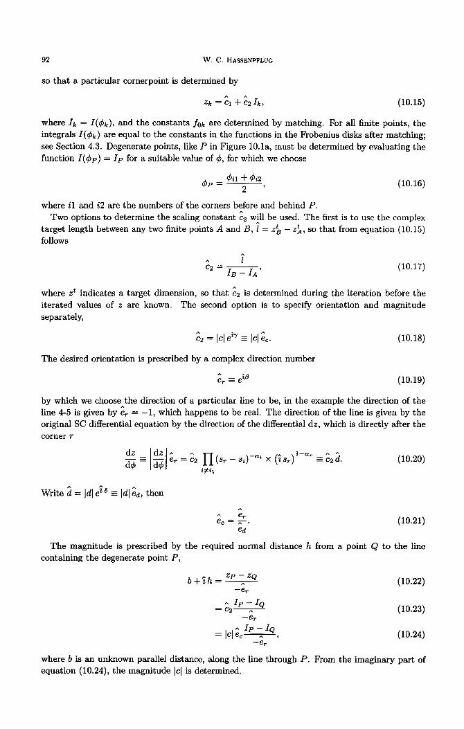
92 W . C . HASSENPFLUG
SO that a particular cornerpoint is determined by
^
Z k = C l "~- C2 I k , (10.15)
where I k = I(¢k), and the constants fOk are determined by matching. For all finite points, the integrals I ( ¢ k ) are equal to the constants in the functions in the Frobenius disks after matching; see Section 4.3. Degenerate points, like P in Figure 10.1a, must he determined by evaluating the function I ( ¢p ) = I p for a suitable value of ¢, for which we choose
¢~1 + ¢i2 Cv = 2 ' (10.16)
where i l and i2 are the numbers of the corners before and behind P. ^
Two options to determine the scaling constant c2 will be used. The first is to use the complex target length between any two finite points A and B, 1 = z~ - z~, so that from equation (10.15) follows
C 2 I B -- I A ' (10.17)
where z t indicates a target dimension, so that c2 is determined during the iteration before the iterated values of z are known. The second option is to specify orientation and magnitude separately,
c2 = Icl e " - I c l ;c. (lO.18)
The desired orientation is prescribed by a complex direction number
^
er -- e ~f~ (10.19)
by which we choose the direction of a particular line to be, in the example the direction of the ^
line 4-5 is given by e r -- - 1 , which happens to be real. The direction of the line is given by the original SC differential equation by the direction of the differential dz, which is directly after the corner r
= " ---- c2 d. (10.20) er e2 i y i i l
Write d = ]d[ e ~ -= [d]ed, then
^
^ e r ec = --.^ (10.21)
ed
The magnitude is prescribed by the required normal distance h from a point Q to the line containing the degenerate point P,
b + T h - z p - ̂ ZQ (10.22) - - e r
^ I F - - IQ (10.23) - - C2 .., - - e r
= [el e~ IF -,. IQ , (10.24) - - e r
where b is an unknown parallel distance, along the line through P. From the imaginary part of equation (10.24), the magnitude [c[ is determined.

Elliptic Integrals 93
We are only now ready to determine cl. Let the finite point to be used to fix cl be z~, then from equation (10.15)
c l = - c 2 I o . (10.25)
We may also specify the middle of two points z~ and z~ such that
^ 1 ^ 1 cl = ~ (z b + z}) - c2~(Io + IT). (10.26)
The end effect is the same as equation (10.25). The purpose of equation (10.26) is to get a symmetric display of the iterated polygon on the computer screen during iteration on a PC.
In the iteration loop, we have now arrived at a point that we can determine the cornerpoints from equation (10.15). Independent of the option to determine the constant c2, we want to include any possible dimensions of degenerate points, like h in Figure 10.1a, of which there may be two in the worst case, or even more in rather abstract overlapping polygons. Such dimensions are
^
determined by equation (10.15), where now c2 is already known. All the cornerpoints, including ^ ^
degenerate dimensions, but also cl and c2, are values that vary during the iteration.
This brings us to the beginning of the loop with the new error in equation (10.3). The iteration can proceed once the Jacobian matrix is determined, described below.
10.2. T h e Q u o t i e n t M a t r i x
All numerical Newton-Raphson method approximations employ an approximation of the Ja- cobian matrix by a Quotient matrix, even if indirectly by Chuang et al. [8], or by a packaged solver [3]. The Quotient matrix is
d z e A z e
de LXT"" (10.27)
First we compute the columns of the larger matrix A z n / A ¢ v by solving the SCT by the same routine nv times with positions ¢1, ¢ 2 , . . . , ¢i + A ¢ i , . . . , Ca, subtracting the basic solution zn(-¢n), and dividing by A¢i (hence, Quotient matrix), which is the customary method. Each variation A¢i corresponds to a column
A¢-7 .n = (10.28)
The solution is in terms of the expansions in convergence disks, which only need to cover the circle boundary during iteration. The computational effort in our analytical method is getting the expansions, while the determination of the cornerpoints afterwards is trivial, all n points being available after matching. The evaluation of the series is necessary for the matching, only any degenerate points will require additional series evaluation. Therefore it is no more effort to compute the complete column A z n / A ¢ i than to compute the partitioned column A z e / A ¢ i .
The stepsize A¢i is controlled to ensure both that ¢i + A¢i remains in the available gap, and - - e
tha t the column A z e / A ¢ i is a reasonable finite approximation of the partial derivative Oz d¢~ " The n , expansions and evaluations for matching are the equivalent of the n , x n , numerical
integrations of the numerical method.
The Quotient matrix A z e / A ¢ " is a partition of the independent rows of A z n / A ¢ " with which the Gauss elimination in equation (10.6) can now proceed. But that is not what we are going to do.

94 W.C. HASSENPFLUG
1 0 . 3 . T h e H - M a t r l x
Instead of solving equation (10.5), we solve the overdetermined matrix equation
d z " • d e v = d z n (10.29)
d ~ v
by Gauss elimination with total pivot search. We call this the H-matrix method for short because it is usually introduced in matrix algebra texts under homogeneous equations [49]. The right vector is the difference between iterated computed values of all finite corner points and all target dimensions,
d z n = - - n - t ~ z - z ( 1 0 . 3 0 )
instead of equation (10.3). Therefore, we supply all finite target coordinate dimensions instead of having to determine an independent set at the input stage. The pivot search elimination routine will select exactly nv independent rows, and the solution is unique because the right vector is compatible. But not only will the pivot search select independent rows, it will also select the best conditioned independent rows. In the example of Figure 10.1a, it will select the dimension x2 from both x2 and Y2. If the coordinate axis direction changes, the selection will change. The computational effort is not more since only nv rows are used for computation. The extra computer storage of the larger matrix is trivial compared to the convolution numbers. We have followed the selection of rows by the H-matrix routine in some examples, and found it quite surprising in what sequence a figure can be drawn instead of the sequence described in Section 10.1. The angles and dimensions of a polygon are determined by a problem orientated subroutine, which
^ ^
also computes Cl and c2. Therefore we do not have to give the information to the main program of which dimensions are now redundant, the H-matrix routine will simply eliminate those rows. We
A ^
can change the reference points for Cl and c2 without any information to the main program; the H-matrix routine will just select appropriate other rows. We can also use any other conceivable consistent method to compute Cl and c2 in the problem routine without any effect on the main routine at all. This method also solves the problem of full or almost degenerate vertices of a polygon. We have compared the H-matrix method with the normal determined method and found no difference in performance. But it relieves us of all the constraints of posing the problem dimensions; the H-matrix sorts it out, better than we can prepare it by limited insight.
10.4. F i x p o i n t s
We call a particular distribution of ¢i a constellation. We have made experiments with crowded points in a constellation and found the rather surprising result that crowding does not slow the convergence down, it merely affects the final accuracy, although this end effect is undesirable in itself, and limits the range of problems we can compute. But what we did find is that the choice of the three fixed points on the circle influence the convergence rate very much. As demonstration, we show a typical path of the vector ~ n during iteration projected on the plane ¢3, ¢4 for ill- chosen fixed points in Figure 10.2a. In Figure 10.2b, a typical path for better chosen fixed points is shown, projected on the plane ¢2, ¢4. The starting point is marked by a • in the figures.
As a remedy, it is not sufficient to place evenly distributed fixed points on the circle at the beginning of the iteration, because these may be badly chosen in the final constellation.
Although we may choose best 120 ° spaced fixpoints, a regular 3-pointed star pattern, intu- itively, there is no theory available to confirm this. Therefore we have made some experiments with different problems as follows. We used no fixpoints at all, contrary to Riemann's mapping theorem, and constructed a larger H-matrix Azn/A-¢ n, still containing all the overdetermined rows. The total pivot search in the H-matrix solution covers all rows and columns. We prescribed

Elliptic Integrals 95
2 1 7 ° 2 5 2 o
1 1 2 ° 1 4 7 °
4 0 ° 1 8 0 ° - 2 0 ° 1 2 0 °
(a) Ill-chosen fixpoints. (b) Well-chosen fixpoints.
Figure 10.2. Projected convergence path in C-space.
the rank of the matrix as nv = n - 3 and followed now which three columns are not selected.
These are the fixpoints. The other points were then used in the continuing iteration.
The result was almost as expected. Throughout the iteration, the three fixpoints were always
selected (i.e., omitted in the H-matrix) in almost the regular star pattern. The only strange
result was that within a few degrees not the best possible regular star pattern was selected. Therefore we use the empirically determined rule to use fixpoints as near as possible to a regular
star pattern. This is determined by a search-like routine at each iteration step, and the routine continues with new variable points at each iteration. In this way, we start with a regular star pattern at the beginning and we end with a best approximated one. Perhaps in the future such a rule can be confirmed theoretically, along the lines of condition number of matrices.
We cannot use the larger H-matrix method to determine the fixpoints during the iteration be-
cause we would waste the computation of three extra columns, i.e., three full SCT computations. It was further interesting to find out whether the rank of the larger H-matrix is in fact n - 3.
This was difficult to determine, as the matrices are often quite ill-conditioned, and a suitable small e to determine numerical rank could not be estimated. But towards the end of each iteration the distinction was quite clear; the rank could confidently be established as n - 3, which is actually a numerical verification of Riemann's mapping theorem.
10.5. B i l i n e a r C o n d i t i o n i n g
It has been noted before that an iteration routine like the one above may tend to crowd some
points unfavourably. Trefethen [3] has noted that this can always be alleviated by a MSbius
transformation. But this is too late after convergence. Crowding causes inaccuracies due to small differences in ¢i while ¢ is a potential-like function with a range of 2r.
We have therefore introduced a MSbius transformation, also called bilinear transformation,
after each iteration step. This consists of selecting the two smallest gaps and make them equal
and on opposite positions of a diameter, which makes them a maximum. If the gaps are adjacent, then the maximum will be obtained by an equilateral of the three points on the circle. But this
will make other gaps smaller again. Therefore, the bilinear transformation is done in small increments at a time. A bilinear transformation can be considered as a shift of the center of the circle by a complex number b to another point. We calculate the number b to effect the maximizing of the two smallest gaps, but then transform only by a small fraction Ab. After this, we look for the new two smallest gaps and continue. The process stops if either the two gaps are equal and opposite, or if a third, previously larger, gap becomes as small. We found that with approximately one to five such steps our goal has been achieved. We have not yet made experiments to relate the size of Ab to the number n of the polygon. Each iteration step

96 W . C . HASSENPFLUG
starts then with the best possible condition of a constellation. In the example of Trefethen's Figure 10b [3] (see Figure 5.7b), we get without bilinear conditioning, a smallest gap of 0.05240 ° and an accuracy of 4 • 10-Sh at convergence after 16 iterations, where h is the channel width. With bilinear conditioning, we get two smallest gaps of 2.0082 ° and an accuracy of 5 • 10-Sh at convergence after 15 iterations. The problem gets worse with small gaps; we have constructed a more difficult 6-cornered example, where without bilinear conditioning the smallest gap is .0009 °, which reduced to .04 ° with conditioning. If no better initial information is available, the iteration is started with uniformly distributed points. After convergence, the constellation is unique for each problem, independent of the fixpoints.
We show in Figure 10.3 the projected path of the iterated solution vector with bilinear condi- tioning, with ill-chosen fixpoints in (a) and well-chosen fixpoints in (b), for the same problem. In an alternative graphical display, the convergence of a 12-sided polygon is shown in a (¢, iteration- step)-diagram in Figure 10.4a and Figure I0.4b, without and with bilinear conditioning.
2 5 2 o
o 1 4 7 °
4 0 ° 1 8 0 ° - 2 0 ° 1 2 0 °
(a) Ill-chosen fixpoints. (b) Well-chosen fixpoints.
Figure 10.3. Projected convergence path in ~-space, with bilinear conditioning.
X/Ill~If , \ I \ I I , I I I I i / \ I Ill I/Ill
X/ ///I I \ i l I | / I I I II II [ I
~ I I| I J I1 I f I| I I I| I I
0 o 3 6 0 ° 0 o 3 5 0 °
(a) No bilinear conditioning. (b) With bilinear conditioning.
Figure 10.4. Convergence path (~n, iteration-step).
The small gap and corresponding inaccuracy is also associated with an ill-conditioned Quotient matrix. Results of the used rows of the Quotient matrix and the Euclidean matrix condition number k E , see [46,50], are presented in Table 9.1, for the polygon in Figure 10.1a. In Case (a), bad fixpoints and no bilinear conditioning were applied, and in Case (b), the fixpoints and bilinear conditioning were applied as described above. While the condition number in the latter case is still acceptable, it indicates the trend towards an ill-condition.

Elliptic Integrals 97
Table 9.1.
Condi t ion N u m b e r Gap Quot ien t Mat r ix
kE
.1052708 .0862352 --.0205346
Case (a) 2,8311 ° .0628882 - . 6993138 - .0215445 7.02321
0 .0101056 .650712
1.631816 -1 .068623 -3 .711639
Case (b) .0674 ° -10 .70067 34.51363 -1 .489695 73.0026
9.942525 -29 .60374 1.302242
One might suggest tha t the bilinear conditioning could be incorporated in the Newton-Raphson iteration as a constraint condition. But this is not desirable for two reasons. The first is that in the beginning of the iteration the correction steps d e '~ are quite large, while the bilinear conditioning steps need to be small. The second is tha t there is no need to. Imagining the convergence paths of all possible constellations in Figure 10.3b, then it is clear tha t the previous Newton-Raphson routine always follows the best available path anyway.
10.6. C o n v e r g e n c e D i s k s
The regions in which the different series are valid are the convergence disks. During the iteration, only the covering of circular boundary of the s-plane is necessary. While the P-~obenius disks are prescribed by the centers sai, the remaining gaps must be covered by Taylor or Laurent disks.
The Laurent disks are introduced to prevent too many small Taylor disks start ing from the tiny at crowded points. We have constructed a routine tha t seeks clusters of points that are suitable to be enclosed by a Laurent disk, which is an annulus. Suitability is defined as a prescribed ratio of at least 2 of ro/ri. For each cluster, the Laurent disk information is placed in the Laurent regions table, until all possible clusters are exhausted. By definition of clusters, it may happen tha t Laurent disks lie within another Laurent annulus. The still remaining gaps are covered by Taylor disks. In each gap, as few as possible Taylor disks are placed on the circle, with the constraints of the nearest singular point on either side of the gap, as well as other singularities on the circle. I t is important tha t the numerical radius of convergence is > 0.5 times the theoretical, so tha t consecutive Taylor disks away from a tiny Frobenius disk will become larger.
Any open regions within the unit s-disk are not covered during iteration. At the end of this routine, the disk F1 is chosen as reference and a sequence of match points
is established and entered in a match table to be used when matching of the series is done. For each iteration step, new tables have to be set up. In the Quotient matr ix method, new tables have to be set up even for each difference step. It is therefore imperative that this covering is done automatical ly during iteration.
The boundary disks only have to touch each other. Only for the full disk covering is an overlapping better. Only at the application of the i terated converged result, additional Taylor disks are inserted to cover the remaining open spaces. This is not part of the iteration routine and we have not programmed such a routine. Instead we enter suitable Taylor disk centers as input interactively on the screen. As visual aid, three different colors are used for the three different types of disks. A suitable set is then placed in the data tables; see Section 4.4.
10.7. R e s u l t s
The convergence of the polygon of Figure 10.1a is shown in Figure 10.5a, and tha t of Fig- ure 10.1b in Figure 10.5b. In many practical applications accuracy of 10 -3 is quite sufficient, and
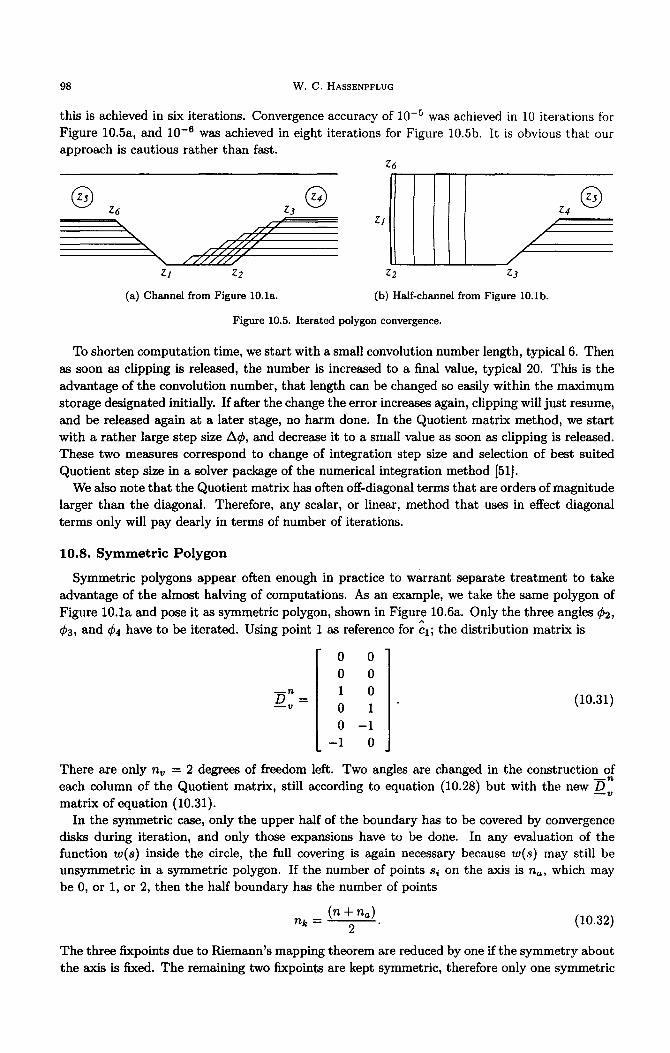
98 W . C . HASSENPFLUG
this is achieved in six iterations. Convergence accuracy of 10 -5 was achieved in 10 iterations for Figure 10.5a, and 10 -6 was achieved in eight iterations for Figure I0.5b. It is obvious that our approach is cautious rather than fast.
z6
@ @ @ Z6 Z3 Z4
Zl Z2 Z2 Z3
(a) Channel from Figure 10.1a. (b) Half-channel from Figure 10.1b.
Figure 10.5. Iterated polygon convergence.
To shorten computation time, we start with a small convolution number length, typical 6. Then as soon as clipping is released, the number is increased to a final value, typical 20. This is the advantage of the convolution number, that length can be changed so easily within the maximum storage designated initially. If after the change the error increases again, clipping will just resume, and be released again at a later stage, no harm done. In the Quotient matrix method, we start with a rather large step size A t , and decrease it to a small value as soon as clipping is released. These two measures correspond to change of integration step size and selection of best suited Quotient step size in a solver package of the numerical integration method [51].
We also note tha t the Quotient matrix has often off-diagonal terms that are orders of magnitude larger than the diagonal. Therefore, any scalar, or linear, method that uses in effect diagonal terms only will pay dearly in terms of number of iterations.
10.8. S y m m e t r i c P o l y g o n
Symmetric polygons appear often enough in practice to warrant separate t reatment to take advantage of the almost halving of computations. As an example, we take the same polygon of Figure 10.1a and pose it as symmetric polygon, shown in Figure 10.6a. Only the three angles ¢2,
^ ¢3, and ¢4 have to be iterated. Using point 1 as reference for Cl; the distribution matrix is
0 0 0 0
- -n 1 0 --Dr = 0 1 (10.31)
0 - 1 - 1 0
There are only nv = 2 degrees of freedom left. Two angles are changed in the construction of - - n each column of the Quotient matrix, still according to equation (10.28) but with the new D matr ix of equation (10.31).
In the symmetric case, only the upper half of the boundary has to be covered by convergence disks during iteration, and only those expansions have to be done. In any evaluation of the function w(s) inside the circle, the full covering is again necessary because w(s) may still be unsymmetric in a symmetric polygon. If the number of points si on the axis is ha, which may be 0, or 1, or 2, then the half boundary has the number of points
(n + no) nk = 2 (10.32)
The three fixpoints due to Riemann's mapping theorem are reduced by one if the symmetry about the axis is fixed. The remaining two fixpoints are kept symmetric, therefore only one symmetric

Elliptic Integrals 99
P
(a) Symmetric dimensions. (b) Symmetric convergence.
Figure 10.6. Symmetric polygon channel.
fixpoint has to be chosen. The degrees of freedom are then
(n -- no) n v - ~ 1. (10.33)
For example, treating the rectangle as symmetric leaves only one degree of freedom which is reflected in the modulus k of elliptic integrals.
The symmetric constellation of ~ n is due to the fact that symmetry can be kept invariant during transformation z(s) . Therefore, the bilinear conditioning must be done by a symmetric routine that searches for the two smallest gaps only above the symmetry axis, and allows only axial displacement Ab.
We have made another set of experiments with a full overdetermined H-matrix of the symmetric points, and it confirmed that the best fixpoint is nearly normal to the axis. It may depend on the number n a o f points on the axis, but it is not worthwhile to make that distinction in the selection of the fixpoint. Therefore, for the symmetric case, another fixpoint routine is implemented that seeks the point nearest to the normal to the axis. Note that the final constellation is independent of the fixpoint. For example, the symmetric triangle, with zero degrees of freedom, will be mapped on equally 120 ° spaced points on the circle due to bilinear conditioning.
The symmetric convergence of the polygon in Figure 10.6a is shown in Figure 10.6b. Accuracy of 10 -3 was achieved in seven iteration steps, and convergence of 10 -6 in nine iteration steps.
10.9. J a c o b i a n M a t r i x
The Jacobian matrix in equation (10.29) is
0zl Ozl
d z n d¢1 d¢n
d e ~ - . (10.34)
Ozn eOzn
d¢1 d¢~
A Jacobian matrix is actually square, therefore we will call the analytical version of the H-Matrix in equation (10.29) the Jacobian H-Matrix if the distinction is necessary.
While the Quotient matrix is computed by known right-hand sides of equation (10.29), for the analytical Jacobian it is the other way round: the partial derivatives are determined first. The partial derivatives are transformed to analytical complex derivatives by the transformation
Ozk Ozk dsj Ozk ^ d C j - dsj d¢ i - ds 3 zsy, (10.35)

100 W . C . HASSENPFLUG
where the complex derivative is the derivative of equation (10.15)
~Zk OC1 0C2 ^ OIk dsj = ds--~. + ~sj Ik + c2 -~sj" (10.36)
But we never use the integrals at the corners sk, which is clear when we review the procedure of Section 4.3 to compute Ik by matching of the series expansions. The integrals Ik are obtained from the series integration without a specific constant first, a function which we designate now by Fk(s), and integration fok constants are found from matching. Let us define the notation
n
F(s) - / H ( s - s,) -a ' ds + fOk, (10.37) i----1
Fk(s) = expansion of the SC-function in disk k,
Fk = Fk(sk),
Ik(s) = Fk(s) +/ok,
Ik = Ik(sk).
At all finite corner points sk the functions Fk(Sk) = 0, and we use point 1 as reference, f01 = 0. Therefore I1 = O, Ik = fOk. If point 1 is an infinite point, we use f01 = 0 anyway. To get the integration constant in a disk at point k from a previous disk in the matching sequence at point r, we use a matching point s,n in the overlapping region, where the series values are set e q u a l , Ik(Sm) = fr(Sm), s o that
fok = Fr(sm) + fOr - Fk(sm).
Therefore, the corner integrals are actually determined by the functions at the matching points by the sequence of matching
11 = 0, (10.38)
12 = F l ( S m ) - F2(8m),
Ik -- Ir = Fr(sm) - Fk(Sm), (10.39)
where sm is a different value in every matching equation. Finite values of Ik in the equations above corresponding to infinite corners are simply ignored in equation (10.15).
Similarly, we define the notation
~Fk dsj = expansion of the Leibniz integral in disk k,
OFk OFk(sk)
dsj dsj '
OIk(S) OFk(s) = ~ + l o k , dsj dsj
oI~ O~k(sk)
dsj dsj '
where the integration constants lOk axe found by the same matching of the Leibniz integral functions. Therefore,
011 dsj = 0, (10.40)

Elliptic Integrals 101
012 OFl(sm) OF2(sm) dsj dsj dsj '
Olk oI~ OFt(sin) OFk(sm) - - - - - - (10.41)
dsj dsj dsj dsj
From equation (10.37)
OF 0 f n dsj - dsj I I ( s - si) -~' ds. (10.42)
i = 1
From Leibniz' formula we get
OF / '~ ds---~ = c~j (s - sj) - ° j - 1 1-I(s - s~) -~ 'ds - Yj(s), (10.4:3)
i#j
which is a SCT integral that can be evaluated by the same method as the original integral iH equation (10.13). Let us refer to the 1.h.s. as the Leibniz derivative, and the r.h.s, as the Leibniz
integral. To our knowledge, no record exists of evaluating the integral in equation (10.43) to obtain the
Jacobian directly. The nearest to a numerical evaluation of the analytical Jacobian is presented by Chuang et al. [8], who give equation (10.42), but do not continue to the Leibniz integral. Instead, they use an interpolation formula to obtain the derivative from five varied computat ions of Ik, which means tha t they use five times as many computat ions as are necessary to compute
the derivative directly from equation (10.43). The Leibniz integrals Jj (s) are computed by convolution numbers in terms of Probenius, Lau-
rent, and Taylor series using the same channels of computat ion as for the basic SC integral. In the computer program, we star t each iteration with one computat ion of the SC integral, with the exponents in equation (10.13), to get the present iterate values of zk. For later reference, we call this stage of the program the direct mode. Then we use the same covering convergence disks, the same transformation
8 - - 8 i u -- , (10.44)
Pi
to compute the Leibniz integral, by simply substituting the exponents of equation (10.13) by those of equation (10.43), and multiplying the result by c~. We call this stage of the program the derivative mode. The Leibniz integrals Jjk = Jj(sk) are finite when the corner zk is finite, and infinite when the corner zk is at infinity, except for the diagonal term ~ = Jkk. The analysis of dsk the diagonal t e rm is presented in Appendix C, including the case c~ = 0.
The derivatives of the constants in equation (10.36) (which should be seen as variationals in this context to avoid a contradiction of terms) are obtained by taking the derivatives of their mode of calculation. From equations (10.17) and (10.15)
,, (91 OI
^ (10.45) ds---~ = -c2 IB -- IA '
then from equation (10.26)
OCl 0c21 ,, 1 (OIo OIT~ ds--'~ = -~sj 2 ( Io- - IT)--c2-2 \-~sj -~sj ] " (10.46)

102 W.C. HASSENPFLUG
The second option for c2 is more complicated. The derivative of equation (10.18) is
dc2 dlCle~ +~ ^ d-~ d C k = dCk c 2 ~ . (10.47)
From the derivative of the logarithm of equation (10.20), and using equation (10.21), we obtain
d ,, d'~ ~sk dCk log ]d I - z ~ k : a k ~ , s r -- sk if r ~ k, (10.48)
~sk ---- Z - ~ i +7 (1 - ~ k ) , if r = k, (10.49)
8k - - s i ~ k
from which d_y_ is obtained by the Imaginary Part of the r.h.s. dCk Taking the derivative of equation (10.23),
db dh ¢k ( Ip - IQ) + c2 dl d l
- - - - ^ (10.50) dCk' + ~ dCk -e~
In this equation, the value h is a given constant, so that d ~ : 0. T h e n ~ is extracted from the known Imaginary Part, which completes the values required for equation (10.36).
Finally, for any degenerate dimension h, we use the Imaginary Part of equation (10.50) again, this time with known ~ , to compute ~ on the 1.h.s.
The derivatives in the Jacobian H-matrix matrix can now be computed by equation (10.35). This matrix is supplied in the place of equation (10.29), while the iteration steps are computed exactly as in the Quotient matrix method.
The problem orientated routine must now Mso supply the information about the details of the different options of specifying the constants cl and c2 so that the appropriate derivatives can be computed in the Main program. Any other options are not permitted unless the derivatives of their construction are added to the Main program. This is quite different from the Quotient matrix Main program which is not concerned about which method is employed.
The symmetric problem routine is much more complicated to construct. The missing Leibniz integrals must be constructed by using certain symmetries. But to obtain these symmetries, the whole complex algebra must be made symmetric as well. For example, the complex logarithms and exponents must be taken on a Riemann plane from -Tr < ¢ < lr. In view of our conclusions in Section 10.10 below, we have not completed such a program.
10.10. Resu|ts
To verify correct computation, the Jacobian matrix was compiled for a symmetric polygon, showing that the elements are consistent within six digits. Comparison with the Quotient matrix showed that the approximations were correct within two to three digits. Yet the convergence was not significantly affected. In the initial iteration stages the steps are clipped anyway, therefore the better accuracy of the Jacobian matrix is ineffective. Towards the end of the iteration, it seems that the limitation of crowded points is more severe than an accurate Jacobian matrix. Perhaps we may still come across ill-conditioned problems where the accuracy of the analytical Jacobian is an advantage. But in the meantime, we conclude that a well-constructed Quotient matrix is just as effective as the analytical Jacobian matrix in the SCT parameter iteration problem. The approximation of the analytical Jacobian matrix by the Quotient matrix as a means of course does not effect the accuracy of the final analytic solution in terms of series as a result.

Elliptic Integrals 103
10.11. E x t e r n a l P o l y g o n
The same Quotient matr ix iteration with the H-matr ix is applied for the iteration of the
external polygon parameters ¢i- In [28], it is stated that the balance to eliminate the residue is
an additional equation to be satisfied in the parameter problem. But with our construction of according to equation (7.7), b is dependent on the parameters ¢i, and is computed merely as one additional step in every iteration as well as every column computat ion of the H-matrix. This is
quite similar to the computat ion of the constants cl and c2. The initial value of b may be hard to find, but the consecutive values during iteration are close enough, due to clipping, to be found quickly.
Therefore, we need the same three fixed points, and the H-matr ix has the same n - 3 columns as for the internal problem. In all practical cases there are no infinity points of the external polygon (see Section 7.1), therefore the H-matr ix consists of the full 2n rows. If there are theoretical infinity points, then there are fewer rows.
The convergence disks must cover the boundary, and there must be a connected sequence to the inner disk at b.
An example of the convergence of an external polygon is shown in Figure 10.7. This is the same example of which the boundary disks are shown in Figure 7.1.
Zlo Zl
Z8 Z9~Z~2 Z3 - % ,
Z7 [ ~ Z4 Z6 Z5
Figure 10.7. Convergence of external polygon.
10.12. P e r i o d i c P o l y g o n
To develop a rational method for the periodic polygon parameter iteration, we consider the remaining independent parameters tha t define the geometric shape of the polygon, if the turning angles c~ are given. To be free from dimensions and orientation, we choose the period p = 1, which is implemented by the scaling constant
^ 1 c2 = ~---, (10.51)
P1
where Pl is the period from the integral before scaling. Starting from point 1, we need one direction relative to p. The the last line through point n is then also fixed, then the polygon is defined by n - 2 lengths in between. Therefore, there are altogether
nv = n - 1 (10.52)
independent parameters, which have to be satisfied by the available parameters in the SCT formula. The available set for variation during iteration is ~ n g, which are n + 2 parameters; therefore, we will have to fix three of these. Note tha t the components of b do not occur as single complex number in equation (8.1). If we consider tha t any variation of these parameters which consti tute a bilinear transformation, will leave the geometry of the polygon invariant; the safest way is to fix the point b during the iteration step. Then we may choose ¢1 as fixed third parameter , or some other measure like ¢1 + ¢n, to fix an axis. In the periodic mapping the

104 W.C. HASSENPFLUG
parameter b has a special influence, somewhat between being free in the internal polygon and
dependent in the external polygon, which causes the unique choice of only one fixed point on the
circle. Note that such a choice allows the same procedure down to the smallest possible number
of n = 2 of the periodic polygon.
To get a better understanding of the influence of the variation of parameters, consider as
example the triangular wave, n = 2, al = 90 °, and a choice of 41 = 0, 4~ = ~r on the circle, as
shown in Figure 10.8a. The triangular wave can then vary with its vertex along a circular arc as
shown in Figure 10.8b. Any variation of b from its shown position along a circular arc through
points 1 and 2, indicated by the dotted line, is a bilinear transformation and will not influence
the triangular wave. The best variation is therefore a variation in a normal direction, along the
shown y-axis. This variation will provide all possible triangular waves with 90 ° vertex. Now we
show how we get exactly the same end result by our iteration procedure, which consists of the following three steps:
• variation of only 42 in the matrix iteration correction;
• bilinear conditioning--this will bring 41 and 42 diagonally opposite each other, and will ^
shift b;
• rotation to bring 41 back to 0.
Y Y
q~2 ~l X Zl Zl
(a) Parameter in the s-plane. (b) Boundary in the z-plane.
Figure 10.8. Mapping of the triangular polygon wave.
We use the same H-matrix method of specifying all 2n coordinates of the n corners with any - - e
infinities left out, in the target array z , and construct the nv = n - 1 columns of the Quotient
matr ix d z as before. d¢
In special cases, no finite length may appear, or perhaps only a very small one. In that case,
a slope of a half-infinite line may be given as coordinate. In exotic cases where infinite lines are included, degenerate dimensions will have to be used. These coordinates are all calculated in the problem subroutine; the quotient matrix will simply consider them as numbers and use the corresponding finite differences.
A typical convergence during iteration is shown in Figure 10.9a (not making use of symmetry), and a potential flow in such a polygon boundary is shown in Figure 10.9b.
10.13. Cyc l i c I n t e r n a l P o l y g o n
The free parameters are the same as for the periodic polygon, nv = n - 1. Therefore, also the central point b and the position 41 are held constant during the iteration step, then bilinear conditioning is applied. The essential difference compared to the periodic polygon is the selection
^
of a norm. Taking the constant cl -- 0 places the center of the polygon at z -- 0 because the

Elliptic Integrals 105
!
92 12 12 92 , | I 2
I I g2
(a) Convergence of periodic polygon. (b) Flow along periodic polygon.
Figure 10.9.
central Frobenius disk is chosen as reference. Then any one point relative to the corners is chosen as fixed. In the example of Section 9.1, the point (Zl + z4)/2 = ~ was chosen. The constant c2 is determined accordingly by
^
c2 ---- (I1 ~- 14)/2' (10.53)
where Ii are the integrals of equations (10.38)-(10.39), in each iteration step and for each Quotient matrix column. All finite coordinates are given as target values for the H-matrix method. Only when exotic infinite corners occur will a slope or degenerate dimension have to be specified.
The smallest number of different corners in a cyclic polygon is n = 1, which is the regular m-sided polygon. No iteration is necessary for only that case.
Convergence during iteration of the example in Section 9.1 is shown in Figure 10.10a. The initial conditions were deliberately set unsymmetric.
D D
(a) Convergence of cyclic internal polygon. (b) Convergence of cyclic external polygon.
Figure 10.10.
10.14. Cyc l i c E x t e r n a l P o l y g o n
The iteration of the cyclic external polygon follows exactly the same iteration routine as the cyclic internal polygon, with the proper negative number m used for the number of cycles.
Convergence during iteration of the example in Section 9.2 is shown in Figure 10.10b, with the same initial conditions as for Figure 10.10a.
33-12-E

106 W . C . HASSENPFLUG
11. C O N C L U S I O N
The Schwarz-Christoffel integral is solved with convolution number algebra for internal, exter- nal, periodic, and cyclic polygons. The solution is analytic, relying on a computer environment. The parameter problem is solved with the quotient H-matrix method which simplifies data input for a specific case. The analytical Jacobian matrix is also obtained, but not found to deliver any bet ter results than a well-groomed quotient matrix method, while being cumbersome in programming and data preparation.
Any SCT solution is not quite sufficient for practical purposes yet. The corners that produce infinities of velocity in potential flow, of temperature, magnetic, electrostatic, or electrodynamic fields are physically not possible. In potential flow, the infinities are avoided by separation, or at least smoothed by a boundary layer. In temperature fields, the material is either dissipating heat or melting away. In magnetic fields, the infinite flux is avoided by oversaturation, altering the potential equation, and in alternating magnetic fields by eddy current heating. In electrodynamic fields, the current is heating up the material until the current density is changed to such a finite value that equilibrium between heating and cooling exists, similar to a boundary layer. In electrostatic fields, the dielectric will break down and released current will flow.
True potential solutions are only possible if the convex corners are rounded. This can be ap- proximated for practical purposes by the replacement of a factor in the SC integrand, see [35]. An example of such use appears in [52]. It is beyond the scope of the present treatise to give an analysis of this method in terms of convolution algebra; suffice it to note that corresponding ad- ditional singularities appear. Whether more elaborate treatment of curvature, as by Floryan [39], can be treated efficiently with convolution number algebra we cannot predict. Alternatively, as practical approximation the close vicinity of a corner may be mapped locally to a corner with a curve if the radius is small.
A further practical application may be the approximation of other than polygon boundaries. This again may be put into two classes. We agree with Trefethen [3] that polygonal approxima- tion of a boundary with a large number of corners renders the parameter iteration impractical, in our case especially so with the convergence disks that convolution algebra requires. In the past, there were such suggestions, as in [6], without actually executing them, although in [17] Costamagna et al. has reported such approximation with up to 100 corners. Instead we propose that a compromise may be useful. Arbitrary boundaries may be surrounded by a polygon, and the SCT will then transform the boundary to a near-circle, from where it can be treated with near-circle iteration methods. For example, all the contours around the external polygon in Fig- ure 7.3a are transformed to circles. In fact, the oldest example is the Joukowski transformation to map an airfoil on a circle. We do not, however, suggest that it may be easy to find a rational method for such an approximation. The computational advantage is that the near-circle region may be sufficiently well approximated by only a central Taylor series. A very short truncated Taylor series has been used by Muskhelishvili [53].
Another class of approximation may be to use the SCT with other than the theoretical SCT sum of angles, resulting in a polygon with curved sides. In Figure 10.11 we show a channel obtained with n = 2 corners, 360 ° on the left end and 180 ° on the right end. In Figure 10.12 we show a curved side polygon which may be used to map a curved boundary with the same angles at the corners to a smooth near-circle boundary.
It is up to the user to decide whether he prefers the existing efficient numerical solutions that are available or the analytical method that we have presented here as a first a t tempt and not quite completc we have not yet got a full-region automatic disk covering routine. To this end, we cannot furnish useful information of computer operating time. Our analytical method has been programmed during the research period and is not optimized. The solution of the parameter problem, in QuickBASIC, takes minutes rather than seconds as reported by Trefethen [3]. During each iteration step we have several screen outputs, particularly color display of all regions and

Elliptic Integrals 107
Figure 10.11. Curved boundary channel. Figure 10.12. Curved boundary octagon.
the present i terated boundary, all of which use time, but during research, t ime well spent in experiencing the mathemat ics graphically, as it were.
A P P E N D I X A
S C A L E D V A R I A B L E
During the large range of proportions of the intervals between singular points of elliptic integrals or the SCT, convergence disks may range from very small radius e to very large radius 1/e. Let the value of the the k th te rm of a series on the edge of a disk with radius r have the value A, which is computed as A = ckr k. During the expansion, the coefficient will therefore be computed as
A A in a small disk, ck = -~g = e~ ,
= A x ek, in a large disk.
In the first case, the coefficient ck may become so large tha t it may overflow long before the end of the convolution number. In the second case, it may become zero before the end of the convolution number, and a multiplication with r k will not recover the value A.
To alleviate this numerical problem, a scaled variable is used in each disk
Z u = - - , (A.1)
Pi
so tha t the coefficient comes into a suitable numerical range ck x pk. For a Taylor and Frobenius disk, we use the radius of the disk as scaling parameter, p = rT and p = rF. For a Laurent disk, we have used the inner radius as scaling parameter, p = ri, which is of the order of the Frobenius disks inside the Laurent annulus.
Consider the integration of a function with scaled variable
-
h = * g d z = p * g d u = p U * f
= U , h ,
where f" = f g and ~ = pf ' . Here we have the choice to evaluate the result as h = p × f ( u ) or as h = hu . In the first case, we have a scaled value f ( u ) available, which may be used to gauge local accuracy. In the second case, we obtain directly an unscaled value of h(u) with global accuracy.
When the inner radius of the Laurent disk ---, 0, the scaling will still be appropriate for the enclosed Frobenius series, but not possible for the Laurent series. Also, considering the Laurent

108 W . C . HASSENPFLUG
series as the product or sum of two independent series which each has a different radius of convergence, a consistent method of two separate scaling parameters can be used. The product
and separation in Section 2.2 must then be adapted to obtain new separated series
a(u) × b(v) = g(u) + h(v). (A.2)
Let the scaled variables be
z u = - , for the Taylor series,
P z
v = - , for the half-Laurent series, -y
and the two series
a(u) = ao + alu + a2 u2 -{- a3u 3 + . . . ,
b(v) = bo + bt + b2 b3
The coefficients of the product can be conveniently displayed as in Figure 2.1, from which it can be shown tha t the separated series
g(u) = go + gxu + g2u 2 + g3u 3 + . . . ,
h(v) = ho + hs + h2 h3 T
have the coefficients
g~ = ~ ai+jbj j=o
hi = ~ ajbi+j j=0
When the scaled variable occurs in the logarithmic series of equation (2.26), the integration constant C tha t was chosen for equation (2.26) depends on the scaling parameter p. This is irrelevant in the series solution of the SCT, where the scaling parameter in each disk is fixed and integration constants are obtained by matching. But when the same function is evaluated with different scaling parameters, the dependency C(p) must be taken into account to obtain the same function values.
Denote the logarithmic series in equation (2.26) by ls(z), and the exponent ~ + m = e,
z -1+¢ dz = __1 + - - =/8( log z). (A.3) ( (
The integral of the scaled variable is, using the same value of the constant C consistently,
/ ( p u ) - l + ~ dz = p~ / ( p u ) - l + ~ du
1 u e = _ _ + p c X - -
£ £
= p e __ + 1 +
= pe/s(log u) +/8(log p). (A.4)
The factor p~ follows directly from the transformation of the differential, but a log-p series, which is the par t /8( log p) in equation (A.4), must be added to keep the integration constant invariant.

Elliptic Integrals 109
A P P E N D I X B S C H W A R Z - C H R I S T O F F E L F O R M U L A FOR THE
S T R A I G H T PERIODIC P O L Y G O N
Let the angles of the polygon in the z-plane be a, b, c , . . . , measured as in Figure 4.1f, and the exponents ~ = a/Tr, j3 = b / r , ~ = c / r , . . . , then
a + / 3 + - / + . . . . 0. (B.1)
The mapped points on the circle in the s-plane are sa = eta, sb -- e ~b, sc -- e~C,.... To obtain a straight periodic mapping we require that the inside of the circle in the s-plane maps into the half-infinite strip in the z-plane; therefore for s --* 0 we require z --~ log s, and dz -d7 --~ 1 / s . The function that satisfies these conditions is
d z ( s - s ~ ) a ( s - Sb)~(S -- Sc) " r ' ' ' (B.2)
ds s
To prove that the function of equation (B.2) satisfies the conditions on the perimeter, we follow the proof as in [31] for the closed polygon. On the circle s = e ¢¢, ds = ~e ¢~ de, therefore
d z = - e a) ° - - de. (B.3)
The factor e ~ cancels. From each term in brackets like ( e ~ - e ~a) extract a factor like e~(C;/2)e ~(a/2) ,
and then separate complex and real factors,
dz = C (sin 2 (¢ - a ) ) ° ( s i n l ( ¢ - b ) ) ~ (sin 1 ( ¢ - c ) ) ~ . . , d~, (B.4)
where the complex constant
= 7 2 ~ e ~(~/2)° 2 ~ e ~(b/2)~ 2 ~ e ~(~/2)~ - - •
and the factor
e i(¢/2)(a+B+'r+' ' ' ) = 1 (B.5)
in view of the sum in equation (B. 1). From here the proof carries on as in [31], that equation (B.4)
is the equation of a straight line segment in the direction of C as long as ¢ > a, b, c . . . . . The angle ¢ changes from 0 to 2~r on the circle. Each time that ¢ becomes larger than the next angle, the factor - 1 is extracted from the sin-term, changing the direction of the segment dz by r a , r~3, r % . . . , at each corner. In the cases where any one of the angles a, b, c , . . . , are outside the range from 0 to 2~r, the appropriate multiple of 27r is subtracted in the sin-terms in equation (B.4).
The customary proof for the cyclic periodic polygon uses a transformation of a 1 / n segment of a circle on the full circle, see [28], which cannot be applied to the straight periodic polygon with infinite n. But the proof for the cyclic polygon can be carried out as above, changing equation (B.1) to the correct sum, 2~r /n for the internal and - 2 r / n for the external polygon, and then dividing in equation (B.2) by a power of s such that equation (B.5), now with an uncancelled factor from equation (B.3), becomes true again. Then it is easy to see that the formula is also true for n not an integer.

i i0 W.C . HASSENPFLUG
A P P E N D I X C D I A G O N A L J A C O B I A N M A T R I X E L E M E N T
In the case of the diagonal of the Jacobian matrix of equation (10.34), the derivative in equa- tion (10.42) is
OFk O f - - dsk J ( s - Sk) -~k H ( S -- Si) -~ ' ds. (C.1)
dSk
From Leibniz' formula we get
n
OFkdsk = ak / (S -- Sk) -~k -1 H ( S -- Si) -~ ' ds. (C.2)
An alternative expression of the derivative is obtained if we do partial integration first and apply Leibniz' formula to the integral in the second term, with the result
= - ( s - H ( s - si)-°, + J ( s - skl ds (c.3/
The fact tha t for finite corners the Leibniz integrals are finite is of no importance because we have to deal with the integral at infinite corners anyway. But there is a different implied constant in the two forms of the derivative. To make this clear, consider the expansion with the transformation
u = s - s k . ( C . 4 )
Then equation (C.2) becomes
°/ / d--s u -~k x U__" g du = ak U - a k - 1 X U " g du
× u. f J(- ak--1)
= akU - ~ x go + --ak + 1 g lu + --ak + + .. (C.5)
~ - g o u -1 + g l l o g u +g2u 2 + -g3u 2 + ' " . (C.6) 1
Equation (C.3) becomes
o/ _ / d-~ u -ak x U . g d u = - u -~k x U . g + u - ~ x U . g ' d u
/(_ - ' = - u -ak x U . g + u -~k+l x U " g (C.7) ak)
= U_a. (_gO nu OLk OLk ) --ak "k 1 g lu + - - g2 u2 -[- . . . (C.8)
--ak + 2
t~k 1 2 1 ) g l l o g u - - g 0 u - 1 - g l + g 2 u 2 + ~ g 3 u + ' ' ' . (C.9)
Equations (C.5) and (C.8) are the same, but equation (C.8) is well determined for ak ~ 0 while equation (C.5) is not. Equation (C.9) differs from equation (C.6) by the constant - g l , generally

Elliptic Integrals l l 1
when a logarithmic term gm log u is present, by the constant -gin. This is a result of the arbitrary constant implied in equation (2.26). Due to matching in equation (10.41), the constant would still be irrelevant were it not for the occasion that the logarithm may occur in the Frobenius series at the reference point 1. To find out which equation to use, we investigate the meaning of
0Ik AIk (C.10)
dsk Ask
as the quotient of two small quantities, true to the meaning of Leibniz' derivative symbol. In Figure C.1, two overlapping convergence disks at points 1 and k are shown with the variations that produce A I k / A s k . In each disk, the transformation u, = s - s, is used for the convergent Frobenius series
P n
F1 = / u - ~ '~' H ( u l + s - s , )du, (C.11) J
I " n
Fk = / u - k '~ H ( U k + S -- s~)du. (C.12) J i#1
The corner integral at point k is determined, according to equation (10.39), by the difference of the functions at the matchpoint
Ik - I1 = Fl(sk, urn1) - Fk(sk, Umk). (C.13)
The matchpoint is sin, which is a distance urn1 from point 1 and a distance Umk from point k, such that s~ = urn1 - "ll, mk. The point k is now moved by the amount dsk to position Sk +dsk . The difference in the functions Fi is due to the change of parameter Sk, but also due to change of distances Umi, therefore
OIk 011 OF1 OF1 [ dural dSk ~Sk = d s k u,,~l (Sk'UmX) "Jr- ~ ] s k ($k,Urnl) X ds--'--'k-
OFk [ OFk dumk (C.14) dsk (Sk,Umk) -- ~ (Sk,Umk) x ds----~"
I ~nk 8k
dsk \
st I
Umk ./ I" / ~" ~.
/ / Um~ - dsk
\ \ /
Figure (?.1. Differentials in 0I / d ~ l k "
We may assume that the matchpoint Sm remains the same. This is no restriction, because according to the convergence of series it does not matter where in the overlapping region the

112 W.C. HASSENPFLUG
matchpoint is chosen. Therefore ~dsk = 0 and ~ask = -1, and equation (C.14) becomes
OIk 011 OF1 [ OFk OFk
dSk ds-k = d s k I (sk, um,)- ~ (sk, umk) + du---~lsk (sk, umk). (C.15) UTnl ~$rnk
The first term in equation (C.15) is the Leibniz integral 0F~ according to equation (10.42), dsk
because Sk appears in one of the product terms. Therefore we remain with the diagonal derivative
OFk _ OFk ~ OFk (C.16) ds~ ~ - du s~'
which applied to equation (C.12) produces
n
OFk f u_~ O i i ( ~ + sk _ 8 , ldu_ u;o~ l-i(u + sk _ s~) d s k = k dsk i~1 i~,
0 n n /-°k l - I ( u + s~ - s , ) , ( c . 1~ ) = ~k ~ H ( ~ + s k - s ~ ) d u - u k iyt l i#I
and these are exactly the terms of equation (C.3) (in reverse sequence) with the transformation of equation (C.4). Therefore, we have the proper from of the diagonal derivative and its geometrical explanation. Equation (C.3) is also well conditioned for ak ~ O. Take, for instance, the example of ak = O. Then
OF, - 0, for all i ~ k including 1,
dsk
OFk dsk : - - g o .
Therefore
oI~ - - 0, for all i ~ k including 1,
dsk
0Ik dsk = - g o .
Geometrically, this means that the polygon remains in the same position and only the degenerate point k moves. This is obvious because the factor of the degenerate point does not appear in the SCT equation. But if a l -- 0, then due to I , = 0, the degenerate point cannot move. Therefore, the whole polygon moves in the opposite direction. The derivatives are now
oF, d81 : - g o ,
OF~ = 0, for all i ~ 1;
dsl
therefore
011 -- 0, by definition,
dSl
oh ds, = go, for all i ~ 1,
as expected.
Elliptic Integrals 113
In our applications, the transformation of equation (C.4) is actually replaced by the scaled variable transformation, see Section 2.4 and Appendix A,
8 -- 8 k u -- (C.18)
P
To get the same Jacobian and Quotient matrix element in equation (C.10) when A s k --* O, we must include the log-p series, see Appendix A, whenever a logarithm or logarithmic series appears in (C.9). But it turns out that due to the differences being taken in equation (10.41), this is not necessary.
R E F E R E N C E S 1. D. Howe, The application of numerical methods to the conformal transformation of polygonal boundaries,
J. Inst. Maths. Applics. 12, 125-136 (1973). 2. W. Squire, Computer implementation of the Schwarz-Christoffel transformation, Journal of the Franklin
Institute 299 (5), 315-322 (1975). 3. L.N. Trefethen, Numerical computation of the Schwarz-Christoffel transformation, SIAM J. Sei. Star. Corn-
put. 1 (1), 82-102 (1980). 4. P. Henrici, Applied and Computational Complex Analysis, Vol. 3. Discrete Fourier Analysis--Cauchy Inte-
grals-Construction of Conformal Maps--Univalent Functions, John Wiley, New York, (1986). 5. E. Costamagna, On the numerical inversion of the Schwarz-Christoffel conformal transformation, IEEE
Transactions on Microwave Theory and Techniques M T T - 3 5 (1), 35-40 (1987). 6. A. Gilicz, Alternative, useful conformal mapping method can be used for odd-shaped fields, Oil 8¢ Gas
Journal 85 (23), 57-58, 60, 62 (1987). 7. M.A. Chaudhry and R. Schinzinger, Numerical computat ion of the Schwarz-Christoffel t ransformation param-
eters for conformal mapping of arbitrarily shaped polygons with finite vertices, COMPEL, The International Journal for Computation and Mathematics in Electrical and Electronic Engineering I I (1), 263-275 (1992).
8. J.M. Chuang, Q.Y. Gui and C.C. Hsiung, Numerical computation of Schwarz-Christoffel t ransformation for simply connected unbounded domain, Computer Methods in Applied Mechanics and Engineering 105, 93-109 (1993).
9. L.H. Howell and L.N. Trefethen, A modified Schwarz-Christoffel transformation for elongated regions, SIAM g. Sci. Stat. Coraput. 11 (5), 928-949 (1990).
10. T.A. Driscoll, Algorithm 756: A MATLAB toolbox for Schwarz-Christoffel mapping, ACM Transactions on Mathematical Software 22 (2), 168-186 (1996).
11. D.P. Levinson and A.D. Snider, Optimal trim patterns for low current noise, The International Journal for Hybrid Mieroelectronics 11 (4), 77-80 (1988).
12. ~. Koq and P.F. Ordung, Schwarz-Christoffel transformation for the simulation of two-dimensional capaci- tance,, IEEE Transactions on Computer-Aided Design 8 (9), 1025-1027 (1989).
13. E. Costamagna and A. Fanni, Asymmetric TEM cell impedance calculation, IEEE Proceedings, (Technical Memorandum) 137 (5), 35-40 (1990).
14. E. Costamagna and A. Fanni, Analysis of rectangular coaxial structures by numerical inversion of the Schwarz-Christoffel transformation, IEEE Transactions on Magnetics 28 (2), 35-40 (1992).
15. J.-S. Yang and C.-R. Chang, Magnetic field of an asymmetric ring head with an underlayer, IEEE Transac- tions on Magnetics 29 (2), 2069-2072 (1993).
16. M.A. Martens, R.W. Brown and E.M. Haacke, Conformal mapping analyses of microstrips with circular and elliptic cross-sections, IEEE Transactions on Microwave Theory and Techniques 40 (9), 1836-1840 (1992).
17. E. Costamagna, A. Fanni and M. Usai, Slab line impedances revisited, IEEE Transactions on Microwave Theory and Techniques 41 (1), 156-159 (1993).
18. V.B. Minuhin, A general solution for the field of polygonal electromagnet, IEEE Transactions on Magnet- ics 29 (6), 4121-4141 (1993).
19. M.D. Meyerson, Conformal mapping and fracture mechanics, Engineering [Yacture Mechanics 41 (6), 951-953 (1992).
20. W.C. Hassenpfiug, Convolution number, Computers Math. Applic. 26 (11), 3-135 (1993). 21. P.F. Byrd and M.D. Friedman, Handbook of Elliptic Integrals for Engineers and Scientists, Springer, Berlin,
(1971). 22. M. Abramowitz and I.A. Stegun, Handbook of Mathematical Functions, Dover, New York, (1972). 23. F. Riegels, Formeln und Tabellen fiir ein in der r~iumlichen Potentialtheorie auftretendes elliptisches Integral,
Archly der Mathematik 2, 117-125 (1949/50). 24. D. Kiicheman and J. Weber, Aerodynamics of Propulsion, McGraw-Hill, New York, (1953). 25. R. Bulirsch, Numerical calculation of elliptic integrals and elliptic functions, Numerische Mathematik 7,
78-90 (1965). 26. R. Bulirsch, Numerical calculation of elliptic integrals and elliptic functions, II, Numerische Mathematik 7,
353-354 (1965).

114 W.C. HASSENPFLUG
27. T.F. Lemczyk and M.M. Yovanovich, Efficient evaluation of incomplete elliptic integrals and functions, Com- puters Math. Applic. 16 (9), 747-757 (1988).
28. W. yon Koppenfels and F. Stallmann, Praxis der Konformen Abbildung, Die Grundlehren der Mathematis- chen Wissenschaften, Bd. 100, Springer, Berlin, (1959).
29. L.M. Milne-Thomson, Plane Elastic Systems, Springer, Berlin, (1968). 30. P.V. O'Neii, Advanced Engineering Mathematics, 3 rd Edition, PWS Publishing, Boston, (1993). 31. L.M. Milne-Thomson, Theoretical Hydrodynamics, 5 th Edition, Macmillan, London, (1968). 32. R.V. Churchill, Complex Variables and Application.s, 2 nd Edition, McGraw-Hill, New York, (1960). 33. E.T. Copson, Theory of b~nctions of a Complex Variable, Oxford University Press, (1935). 34. Z. Nehari, Conformal Mapping, Dover, New York, (1975). 35. P. Henrici, Applied and Computational Complex Analysis, Vol. 1. Power Series--Integration--Conformal
Mapping--Location of Zeros, John Wiley, New York, (1974). 36. A. Betz, Konforme Abbildung, 2 nd Edition, Springer, Berlin, (1964). 37. D. Gaier, Konstruktive Methoden der Konformen Abbildung, Springer, Berlin, (1964). 38. J.M. Floryan, Conformal-mapping-based coordinate generation method for channel flows, Journal of Com-
putational Physics 58, 229-245 (1985). 39. J M. Floryan, Conformal-mapping-based coordinate generation method for flows in periodic configurations,
Journal of Computational Physics 62, 221-247 (1986). 40. L.C. Woods, The Theory of Subsonic Plane Flow, Cambridge, (1961). 41. H. Kober, Dictionary of Conformal Representations, Dover, New York, (1957). 42. L.I. Volkovyskii, I.G. Lunts and I.G. Aramanovich, A Collection of Problems on Complex Analysis, (Trans-
lated by J. Berry), Pergamon, Oxford, (1965). 43. E. Jahnke, F. Emde and F. I2~h, Tables of Higher i~unctions, 6 th Edition, Stuttgart, (1960). 44. E.D. Rainville, Special ~unctions, Chelsea, New York, (1960). 45. J. Todd, Editor, Survey of Numerical Analysis, McGraw-Hill, New York, (1962). 46. L. Collatz, bhnktionanall/sis und Numerische Mathematik, Springer, Berlin, (1968). 47. S.P. Timoshenko and J.N. Goodier, Theory of Elasticity, (Reissue), McGraw-Hill, New York, (1987). 48. Y.S. Kim and H.J. Eom, Fourier-transform analysis of electrostatic potential distribution through a thick
slit, IEEE Tbznsactions on Electromagnetic Compatibilty 38 (1), 35-40 (1996). 49. R. Znrmiihl, Matrizen, Springer, Berlin, (1964). 50. R.A. Horn and C.R. Johnson, Matrix Analysis, Cambridge, (1985). 51. IMSL User's Manual, IMSL Customer Relations, Houston, (1984). 52. R. Ramaswami and H.C. Lin, Simulation of time-dependent tunneling characteristics of MOS structures,
Solid State Electronics 34 (3), 291-299 (1991). 53. N.I. Mnskhelishvili, Some Basic Problems of the Mathematical Theory of Elasticity, (English Translation by
J.R.M. Radok), Noordhoff, Groningen, (1953).