Embed Size (px)
Citation preview
CONTRACTOR
REPORT
TABLES OF ELLIPTIC INTEGRALS
by U?iZl.imz Joel NeZZis
$ Prepared under Grant No. NsG-293 by
i IOWA STATE UNIVERSITY I 1 Ames, Iowa
! NATIONAL AERONAUTICS AND SPACE ADMINISTRATION . WASHINGTON, D. C. . AUGUST 1965
https://ntrs.nasa.gov/search.jsp?R=19650021539 2020-04-08T18:46:41+00:00Z

TECH LIBRARY KAFB, NM
0099785 NASA CR-289
TABLES OF ELLIPTIC INTEGRALS
By W illiam Joel Nellis
Distribution of this report is provided in the interest of information exchange. Responsibility for the contents resides in the author or organization that prepared it.
Prepared under Grant No. NsG-293 by IOWA STATE UNIVERSITY
Ames, Iowa
for
NATIONAL AERONAUTICS AND SPACE ADMINISTRATION
For sole by the C!eoringhouse for Federal Scientific and Technical Information Springfield, Virginia 22151 - Price $2.00


TABLE OF CONTENTS
I. INTRODUCTION
II. DEFINITION AND PROPERTIES OF THE R FUNCTION
III. DESCRIPTION OF TABLE 1
IV. DESCRIPTION OF TABLES 2 AND 3
V. DESCRIPTION OF TABLE 4
VI. EXAMPLES
VII. TABLES
VIII. LITERATURE CITED
IX. ACKNOWLEDGEMENTS
X. APPENDIX: FORTRAN SUBROUTINE PROGRAM FOR COMPUTING RF
AND RG BY MEANS OF DESCENDING GAUSS OR ASCENDING
TANDEN TRANSFORMATIONS
Page
1
2
8
10
13
14
22
41
42
43
. . . 111
--____---~ _ .-

LIST OF TABLES
Table Page
1 Integrals with algebraic or trigonometric integrands 22
2 Reduction formulas for complete integrals of the first 25 and second kinds
3 Reduction formulas for incomplete integrals of the 29 first and second fcinds
4a Numerical table of $(x,y,l) 35
4b Numerical table of RG(x,y,l) 38
iv

I. INTRODUCTION
The tables present a method of evaluating el .liptic integrals of the
first and second kinds by means of the R function, a hypergeometric
function of several variables (1). The general method is to reduce an
integral of elliptic type to an R function by means of the integral
formulas of Table 1. The formulas of Table 2 (for complete integrals)
or Table 3 (for incomplete integrals) are then used to reduce the R
function to a linear combination of two standard R functions and an
algebraic function. The two standard functions 4 and RR (in the complete
case) or RF and R G (in the incomplete case), are normal elliptic integrals
of the first and second kinds (2). Table 4 gives numerical values of the
normal integrals over a limited range; it is intended only to give an
idea of the behavior of the functions and should not be used for inter-
polation near x = 0 or y = 0.
Table 1 can also be used to express elliptic integrals of the third
kind (as well as many other integrals) in terms of the R function, but
tables for reduction and numerical evaluation of integrals of the third
kind are not included. Until such tables are developed, the reader is
referred to conventional tables of elliptic integrals, for example (3,
4, 5), which deal with integrals of all three kinds. For integrals of
the first two kinds, it is believed that the present scheme of reduction
offers significant advantages in conciseness.
. . . ___ ,.___ - -
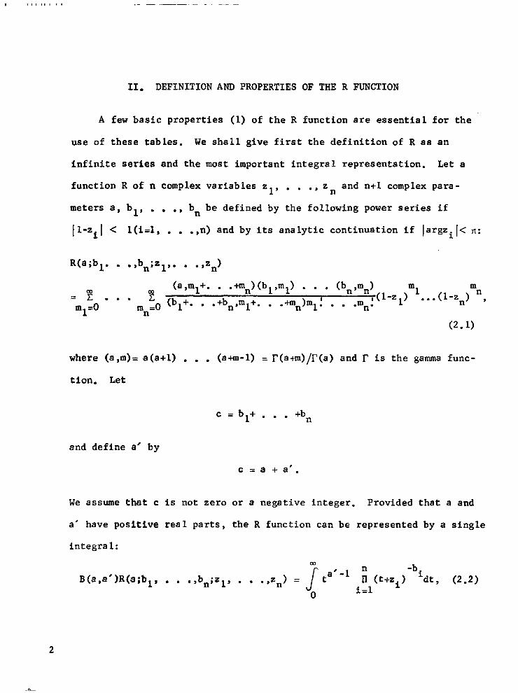
II. DEFINITION AND PROPERTIES OF THE R FUNCTION
A few basic properties (1) of the R function are essential for the
use of these tables. We shall give first the definition of R as an
infinite series and the most important integral representation. Let a
function R of n complex variables 21, . . . , z n and n+l complex para-
meters a, bl, . . . , bn be defined by the following power series if
11-zi1 < l(i=l, . . .,n) and by its analytic continuation if largzil< n:
R(a;bl. . .,bn;sl,. . . ,nn)
=“c... “c (a,ml+. . .+m,)(bl,ml) l . . (b, ,mJ ml
m =O 1 mn=O (bl+. . .+bn,ml+. . .+m,)ml! . . .mn! (l-=1) l l l (l-‘n,““’
(2.1)
where (a,m)= a(a+l) . . . (a+m-1) = r(a+m)/r(a) and r is the gamma func-
tion. Let
c = bl+ . . . +bn
and define a* by
c = a + a’.
We assume that c is not zero or a negative integer. Provided that a and
a’ have positive real parts, the R function can be represented by a single
integra 1: cd
B(a,a’)R(a;bl, . . .,bn;al, . . .,zn) = s
ta ‘-’ ; (t+z )-bidt , (2.2) 0 iA i
2

where B(a,a') = r(a)r(a')/r(c) is the beta function.
The R function has two important properties, symmetry and homogeneity.
Symmetry is apparent from either representation: R(a;bl, . . .,b,;
=y. - .,zn) is invariant under permutation of the subscripts 1, . . .,n,
that is, R does not change when the b's and z's are permuted together.
A scale factor common to all the z's can be removed by changing the
variable of integration in 2.2. Thus, R is homogeneous of degree -a
in the variables z 1, . . ., zn:
W;bl, . . .,bn;szl, . . .,szn) = seaR(a;bl, . . .,bn;zZ, . . .,zn).
(2.3)
This property is often used to make all the arguments of an R function
less than or equal to unity.
The substitution t = r -1 in 2.2 leads to the Euler transformation,
which allows us to change the value of the a-parameter:
n R(a;bl,. . .,bn;zl,. . -,zn)=( R zi
-bi i=l
)R(a';bl,. . .,bn;zlW1,. . .,zn-1).
(2.4)
For the case n = 2, there is another relation which can be used to change
the value of the a-parameter:
a2ka;bl,b2;El,Z2) = z2 bkbl;a,a’ ;y,z2) . (2.5)
Equation 2.5 has no analogue for n > 2. Equations 2.3, 2.4, and 2.5 are
actually valid without restriction on a or a'.
3
h

There are a few special cases of the
provide very useful relations. If one of
zero, say bn, then
parameters and variables which
the b-parameters in 2.1 is
(bn ,mi) = (0, mi) = C m o
i
' is a Kronecker delta, and
R(a;bl,. . . .,bnSl,O;zl,. . . .,z.)=R(a;bl,. . . .,bn-l;zl,. . . .,zn-1).
(2.6)
If any two arguments are equal, say zl = z2, then 2.2 shows that
R(a;bl,. . .,bn;z2,z2,z3,. . . .+.,I
= R(a;bl+b2,b3,. . .,bn;z2,. . . ,q. (2.7)
If any one of the arguments vanishes, say zl, 2.2 again shows that
B(a,a')R(a;bl,. . .,bn;0,z2,. . .,zn)
= B(a,a'-bl)R(a;b2,. . .,bn;z2,. . .,z,),
(2.8)
provided that Re(a'-bl) > 0.
Tables 2 and 3 were derived from recursion formulas for the R
function. Let
R = R(a;bl,. . .,bn;zl,. . .,zn),
R(aLl) = R(a+l;bl,. . .,b,;zl,. . .,zn),
R(bi+l) = R(a;bl,. . .,bifl,. . .,bn;zl,. . .,zn).
4
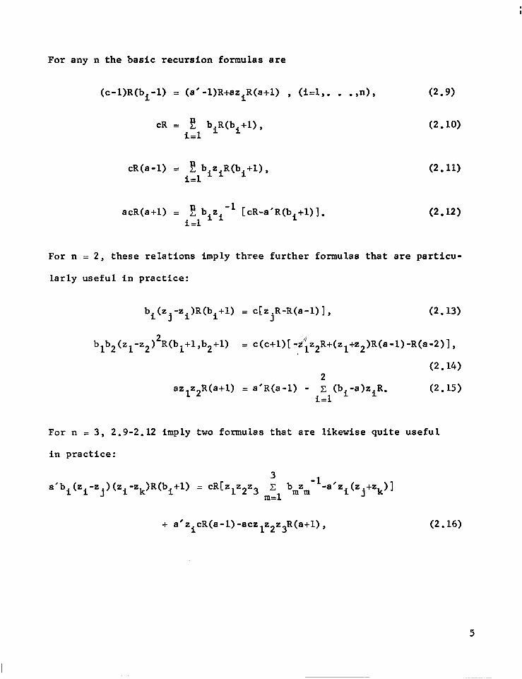
For any n the basic recursion formulas are
(c-l)R(bi-1) = (a'-l)R+aziR(a+l) , (id,. . .,n), (2.9)
CR = 5 biR(bi+l), I=1
(2.10)
cR(a-1) = i~~izi~(bi+l), (2.11)
acR(a+l) = 2 b.z." [CR-a'R(bi+l)]. 14 = 1
(2.12)
For n = 2, these relations imply three further formulas that are particu-
larly useful in practice:
b,(z,-zi)R(bi+l) = c[zjR-R(a-l)], (2.13)
blb2(zl-z2)2R(bl+l,b2+l) = c(c+l)[-,3'iz2R+(zl+z2)R(a-l)-R(a-2)],
(2.14) 2
azlz2R(a+l) = a'R(a-1) - c (bi-a)ziR. (2.15) I=1
For n = 3, 2.9-2.12 imply two formulas that are likewise quite useful
in practice:
3 a'bi(Zi-Zj) (Zi k -z )R(bi+l) = cR[zlz2z3 c
m=l bmzm -l-a'zi(zj+zk)]
+ a'zicR(a-1)-aczlz2z3R(a+l), (2.16)
5
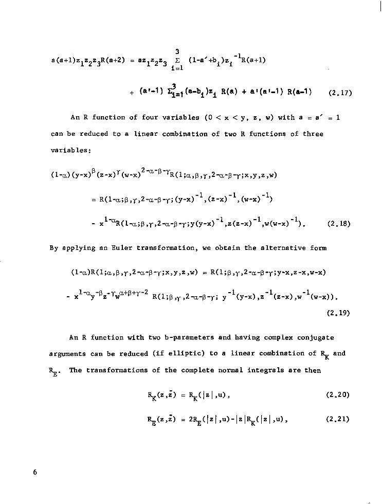
3 a(a+l)zlz2z3R(a+2) = azlz2z3 Xl (l-a'+bi)zi -lR(a+l)
+ fa’-l ) <=I @-bibi R(a) + aI (al-1 ) R(a-1) (2.17)
An R function of four variables (0 < x < y, z, w) with a = a' = 1
can be reduced to a linear combination of two R functions of three
variables:
(l-a) (y-x)B (z -x>r(w-x)2 - a-p-rR(1;o,B,y,2-a-P-y' ,X,Y ,= ,w)
= R(1-a;@,$-a-p-y;(Y-x) -l,(z-x)-l,(w-x)-l>
- +w-a;p ,yJ-a-j3-y;y(y-x) -l,z(z-x)-l,w(w-x) -5. (2.18)
By applying an Euler transformation, we obtain the alternative form
Wa)W;a,13,y,2 -a-P-~;x,Y,z,w) = R(l;p,y-,2-a-p-y;y-x,z-x,w-x)
- x l-uy-pz-rwu+p+y-2 R(l;P ,y ,2-u-B-y; y -+y-x) ,z-l(z-x) ,w-fw-x)).
(2.19)
An R function with two b-parameters and having complex conjugate
arguments can be reduced (if elliptic) to a linear combination of RR and
% The transformations of the complete normal integrals are then
'k((Gl = R-&l,u), (2.20)
%(z,z’> = 2%+1 ,u)-~+~(IzI ru), (2.21)
6
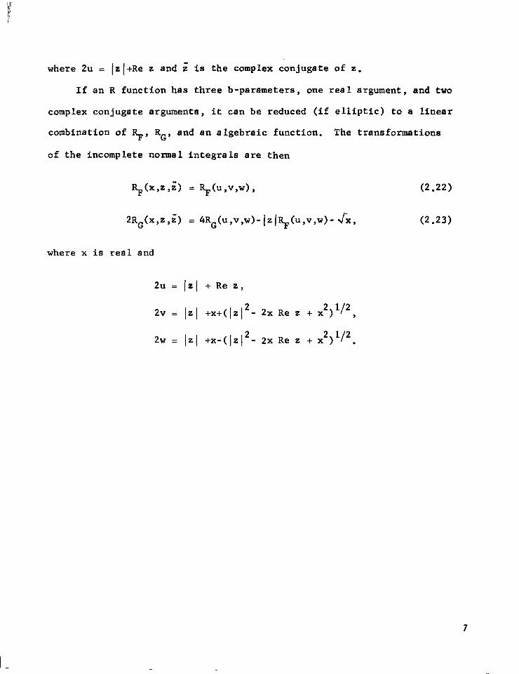
where 2u = IzI +Re z and z' is the complex conjugate of z.
If an R function has three b-parameters, one real argument, and two
complex conjugate arguments, it can be reduced (if elliptic) to a linear
combination of %' RG' and an algebraic function. The transformations
of the incomplete normal integrals are then
$(x,z ,a = ~(u,v,w) , (2.22)
2RG(x,z,G) = 4RG(u,v,w)-Iz(R+,v,w)-A, (2.23)
where x is real and
2u = IzI + Re
2v = IZI +x+(
2w = IZI +x-(
z,
lz12- 2x Re z + x2)li2 ,
H2- 2x Re z + x2)1i2 .
7
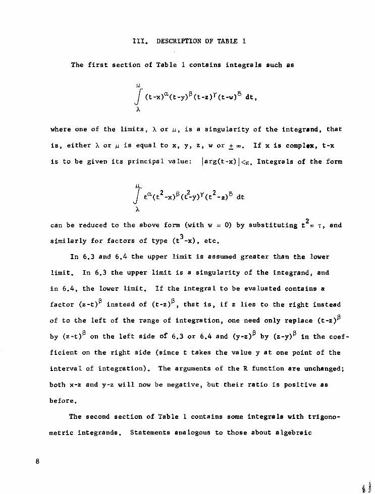
III. DESCRIPTION OF TABLE 1
The first section of Table 1 contains integrals such as
?- J (t-x)“(t-y)B(t-z)r(t-w)’ dt,
A
where one of the limits, A or I-(, is a singularity of the integrend, that
is, either A or p is equal to x, y, z, w or + 00. If x is complrx, t-x
is to be given its principal value: Jarg(t-x) 1 CR. Integrals of the form
P
s t”(t2-x)P(t2-y)r(t2-z)6 dt
x
can be reduced to the above form (with w = 0) by substituting t2= T, and
similarly for factors of type (t3-x), etc.
In 6.3 and 6.4 the upper limit is assumed greater than the lower
limit. In 6.3 the upper limit is a singularity of the integrand, and
in 6.4, the lower limit. If the integra 1 to be evaluated contains a
factor (z-t)B instead of (t-z)P, that is, if z lies to the right instead
of to the left of the range of integration, one need only replace (t-z) P
by (z-t)’ on the left side of 6.3 or 6.4 and (y-z)’ by (z-y>B in the coef -
ficient on the right side (since t takes the value y at one point of the
interva 1 of integration). The arguments of the R function are unchanged;
both x-z and y-z will now be negative, but their ratio is positive as
before.
The second section of Table 1 contains some integrals with trigono-
metric integrands. Statements analogous to those about algebraic
8

integrals can also be made about trigonometric ones. For example, in 6.7
if (1-pcos$) is negative, replace (1-pcos0)' by (pcose-1)' on the left
hand side and (1-p)' by (p-1)' in the coefficient of R on the right hand
side. The arguments of the R function are unchanged; both l-pcosQ and l-p
will now be negative, but their ratio is still positive.

IV. DESCRIPTION OF TABLES 2 AND 3
Table 2 (the complete case) expresses a number of R functions with
half-integral a- and b-parameters as linear combinations of two R func-
tions, RK and RE, which are taken as normal elliptic integrals of the
first and second kinds, respectively:
RK(X’Y) = R+;+,+;x,y),
R.&Y) = R(-+;$;x,y).
Table 3 (the incomplete case) expresses a number of R functions with half
integral a- and b-parameters as linear combinations of three standard R
functions, rj o e of which is algebraic:
R&Y,z) = R++,+,+,Y,z),
RG(x,~,z) = R( -+;~,~,+,Y ,z) ,
(xyz)-1/2 3 111 = R(~;~~~;x,Y ,z).
Each complete integral is a multiple of an incomplete integral with one
vanishing argument, as shown by 2.8:
2RF(x,y,0) = n RK(x,y), (4.1)
4RG(x,y,0) = IT R.#,Y). (4.2)
We are concerned primarily with R functions in which all the
parameters a, bl, . . ., bn are half-integral or integral. If the a-
10

parameter is a negative integer, the series 2.1 terminates and the R
function is a polynomial. If a' is a negative integer, the Euler trans-
formation 2.4 shows that R is then algebraic. A number of such cases
are included in Table 3( the coefficients multiplying the normal elliptic
integrals being zero), but they cannot arise from single integrals of
the type in Table 1, since the integral representation 2.2 converges only
if a and a' have positive real parts.
Excluding such algebraic cases, we have the following rules of thumb:
(1) If n = 2 and all parameters but the c-parameter are half-
integral, we have a complete elliptic integral of the first or second
331 kind; e.g., R(~;~,~;x,y).
(2) If there are three b-parameters, all half-integral, and if
one of the pair (a,a') is a half integer (the other being an integer),
we have an incomplete elliptic integral of the first or second kind;
1311 e.g., R(y;~,~,px,y,z>.
(3) If there are three b-parameters, two half-integral and one
integral, and if the a-parameter is half-integral, we have a complete
elliptic integral of the third kind; e.g., R(i;i,$,l;x,y,z).
(4) If there are four b-parameters, three half-integral and one
integral, we have an incomplete elliptic integral of the third kind;
1111 e.g., R(~;T,~,'~-,~;w,x,Y,z).
(5) If we have four b-parameters, all half-integral, and if a =
a' = 1, we have an incomplete integral of the first or second kind; 1111
e.g., R(~;~,~,T,~;w,x,Y,z).
11
There are many R functions which fall into one of these classes
only after being subjected to some (perhaps quadratic or cubic) trans-
formation. For example, R($$,i; x,y) is a complete elliptic integral of
the first kind.
Table 2 gives some reduction formulas for class (1) in which the c-
parameter is positive and the largest b-parameter is 3/2. Table 3 gives
some reduction formulas for class (2). Equation 2.18 reduces R functions
of class (5) to two R functions of class (1) or (2). If an R function is
not found in Table 2 or 3 but falls into class (1) or (2)) one can extend
these tables by use of 2.9-2.17, especially by 2.13-2.15 in the complete
case and by 2.16 and 2.17 in the incomplete case.
12
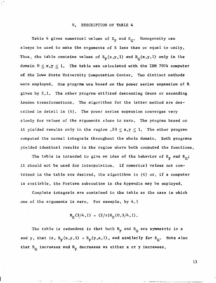
V. DESCRIPTION OF TABLE 4
Table 4 gives numerical values of RF and RG. Homogeneity can
always be used to make the arguments of R less than or equal to unity.
Thus, the table contains values of RF(x,y,l) and RG(x,y,L) only in the
domain 0 < x,y < 1. The table was calculated with the IBM 7074 computer
of the Iowa State University Computation Center. Two distinct methods
were employed. One program was based on the power series expansion of R
given by 2.1. The other program utilized descending Gauss or ascending
Landen transformations. The algorithms for the latter method are des-
cribed in detail in (6). The power series expansion converges very
slowly for values of the arguments close to zero. The program based on
it yielded results only in the region .20 6 x,y 5 1. The other program
computed the normal integrals throughout the whole domain. Both programs
yielded identical results in the region where both computed the functions.
The table is intended to give an idea of the behavior of RF and RG;
it should not be used for interpolation. If numerical values not con-
tained in the table are desired, the algorithms in (6) or, if a computer
is available, the Fortran subroutine in the Appendix may be employed.
Complete integrals are contained in the table as the case in which
one of the arguments is zero. For example, by 4.1
%(3/4,1) = (2/n)RF(0,3/4,1).
The table is redundant in that both % and RG are symmetric in x
and Y, that is , R-+Y,l) = yY,x,l), and similarly for RG. Note also
that RG increases and RF decreases as either x or y increases.
13
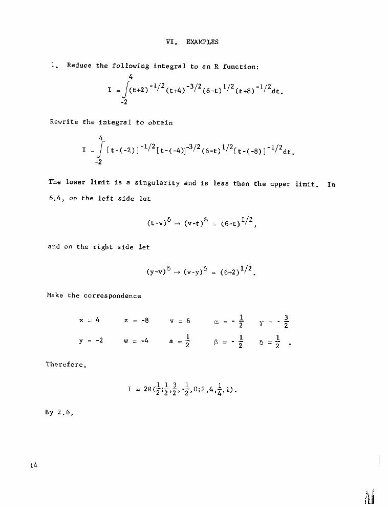
VI. EXAMPLES
1. Reduce the following integral to an R function: 4
I = J
(t+2) -1/2(t+4)-3/2(6-t)1/2(t+8)-1~2dt. -2
Rewrite the integral to obtain
4
I- J
[t+2)]-1/2[t-(-4)]-3/2(6-t)1/2[t-(-8)]-1/2dt.
-2
The lower limit is a singularity and is less than the upper limit. In
6.4, on the left side let
(t-v>6 -+ (v-t)" = (6-t) v2 ,
and on the right side let
(Y-VP 6 4 (v-y) = (6+2>li2.
Make the correspondence
x :: 4 z = -8 v=6 1 a=-- 2
y = -2 w = -4 1 a -- 2 p=-; s=+ .
Therefore,
1 = 2R(25,2,-p 3 , ,;,U. 1.1 2 1 0.2 4 1
By 2.6,
14

1 = 2R$;p2,-p , ,4 . 1 12 1.2 4 1)
2. Reduce the following integral to an R function:
h
I = s
(t+d)1/2(t-f)1/2(h-t)-1/2dt, - d < f < g C h.
g
Equation 6.3 is appropriate. We have the choice of setting either p, y, or
6 equal to zero. Make the correspondence
y=h w = -d 1 a=-T
x=g v=f p=o s=$ .
Therefore,
I = 2(h-g) 1/2(h+d) 1/2(h-f)1/2R(+;0,++$;~,~,~, 1).
Using symmetry and 2.6 we obtain
I = 2(h-g)1/2(h+d)1/2(h-f)li2 R(+;$,+-+; l,$$ g).
3. Express Legendre's incomplete elliptic integral of the first kind as
an R function. X
I= s
(l-t2)-1/2(1-k2t2)'1/2dt , 0 < k x < 1 , . 0
Substitute t2= 'C to obtain
X2
21= 7 s
-1/2(L-T) -1/2(lmk2T)-1/2dT,
0
15
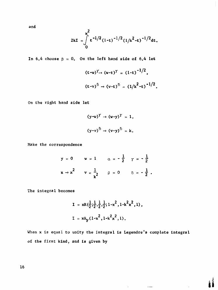
and
X2
2kI= t s
‘V2(1,t) - ‘i2 ( l/k2 -t) ‘l12dt. 0
In 6.4 choose p = 0. On the left hand side of 6.4 let
(t-w& (w-t)Y = (l-t)+*,
(t-v)” -+ (v-t)” = (l/k*+) -l/2 .
On the right hand side let
(y-wp- + (w-yp = 1,
(Y-VP + (v-y) 6 = k.
Make the correspondence
y=o w = 1 C-J, = -- 1 2
2 x3x VIZ-- :2
p=o
The integra 1 becomes
6-i.
1 = N2’2’2’2’ 1.L 1 1. lsx2, lmk2x2, 1) ,
I = x$(1-x2,1-k2x2,1).
When x is equal to unity the integral is Legendre’s complete integral
of the first kind, and is given by
16

I = s(O,l-k2,1), x = 1.
4. Reduce the following integral to a standard R function:
1
I = s
t-1/2(t2+1)-1/2dt.
0
The substitution t2= 7 yields
1 = 2R2(4,4,2~ 9 1.2 1.1 2).
We can obtain an R function whose a- and b-parameters are all half-
integral by reducing the integral to an R with one real argument and two
complex conjugate arguments, and then using the transformation 2.22.
Rewrite the integral as
1
I= .I
t'1/2(t+i)-1/2(t-i)'1/2dt .
0
In 6.4 make the correspondence
x = 1 w = -i 1 a=-- 2 r=-+
y=o v=i p =o s=-$.
The integral becomes
I = 2RR(l+i,l-i,l).
By 2.22,
6
L-
17

I = 2RR(u,v,w),
where
2u &2 + 1
2v = QF2 + 2
2w J2.
5. Reduce the following integral to an R function whose a-parameter
is half-integral:
co
I= s
t112 (t+f)-3/2(t+g)-l/2(t+h)-l/2 dt, f,g,h > 0. 0
In 2.2 make the correspondence
bl+ b3=i a' 2' =-
b2 =$ 5 c =- 2 a = 1.
The integral becomes
31 = 2R(l;~,~,~, 3 L L- f,g,h).
Using the Euler transformation 2.4, we obtain the result,
3f(fgh)l/21 = 2R(;;+,;,$;f-1, g-l, h-l).
6. Express the following R function as another R whose arguments lie
between zero and unity, and then evaluate numerically:
18
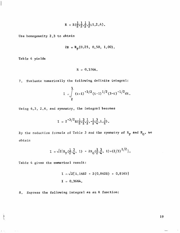
R = R(2,2,2,29 , a L.11 L.1 2 4).
Use homogeneity 2.3 to obtain
2R = $(0.25, 0.50, 1.00).
Table 4 yields
R = 0.3764.
7. Evaluate numerically the following definite integral:
3 I::
s (t+l> -3/2(t-l> 112(3-t) -lj2dt. 2
Using 6.3, 2.6, and symmetry, the integral becomes
By the reduction formula of Table 3 and the symmetry of RR and RG, we
obtain
I = J2[R&,$ 1) - 2R&, 1)+(2/3) II2 ] .
Table 4 gives the numerical result:
I =d2[1.1682 - 2(0.8628) + 0.81651
I = 0.3664.
8. Express the following integral as an R function:
19
. . a . . . . , . , . , , . - . . -
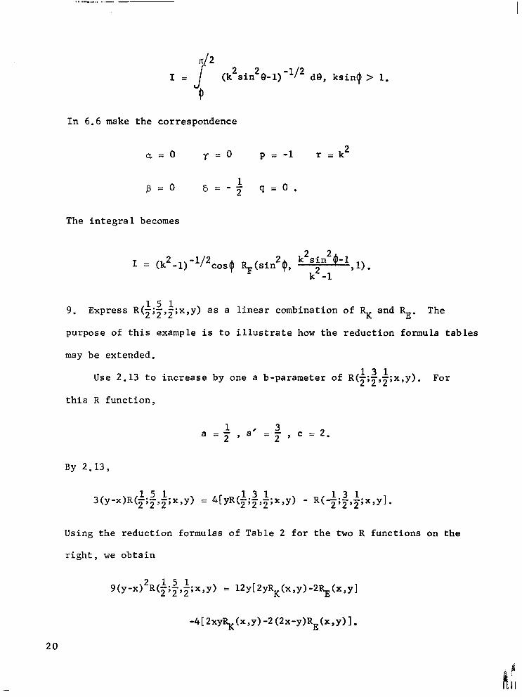
In 6 .6 m a k e th e c o r r e s p o n d e n c e
cc=0 y = o
P 0 =
T h e in tegra l b e c o m e s
IT2 I I= (k2s in2Q- l ) - 1 1 2 d e , ks in$ l> 1 .
P = - 1 r = k2
q = o .
1 = (k2- l ) '1 /2cos$ RF(s in2$, *,l). k2 -1
9 . 1 5 1 Express R ( ~ ;~ ,z;x,y) as a l i near c o m b i n a tio n o f s a n d s. T h e
p u r p o s e o f th is e x a m p l e is to i l lustrate h o w th e r e d u c tio n fo r m u l a tab les
m a y b e e x t e n d e d .
Use 2 .1 3 to i nc rease by o n e a b - p a r a m e te r o f R ( $ ;$ ,+ ;x,y). Fo r
th is R fu n c tio n ,
1 a = - ,a ' 3 2 = - 2 ’ c = 2 .
By 2.13,
3(y-x)R(~;~,~;x,y 1 5 1 > = 4 [yR(+;$+;x,y) - R ( + ;$ ,+ ;x,yl.
Us ing th e r e d u c tio n fo rmu las o f T a b l e 2 fo r th e two R fu n c tio n s o n th e
r ight, w e o b ta in
9(y-x) 2 W 2 L .5 l;x,y) = 1 2 y [2yRK(x,y)-2Rg(x,y] ,2 ,2
- 4 [2 x ~ ~ ( x ,~ ) -2 (2x -~ )R~(x ,~ ) ].
2 0
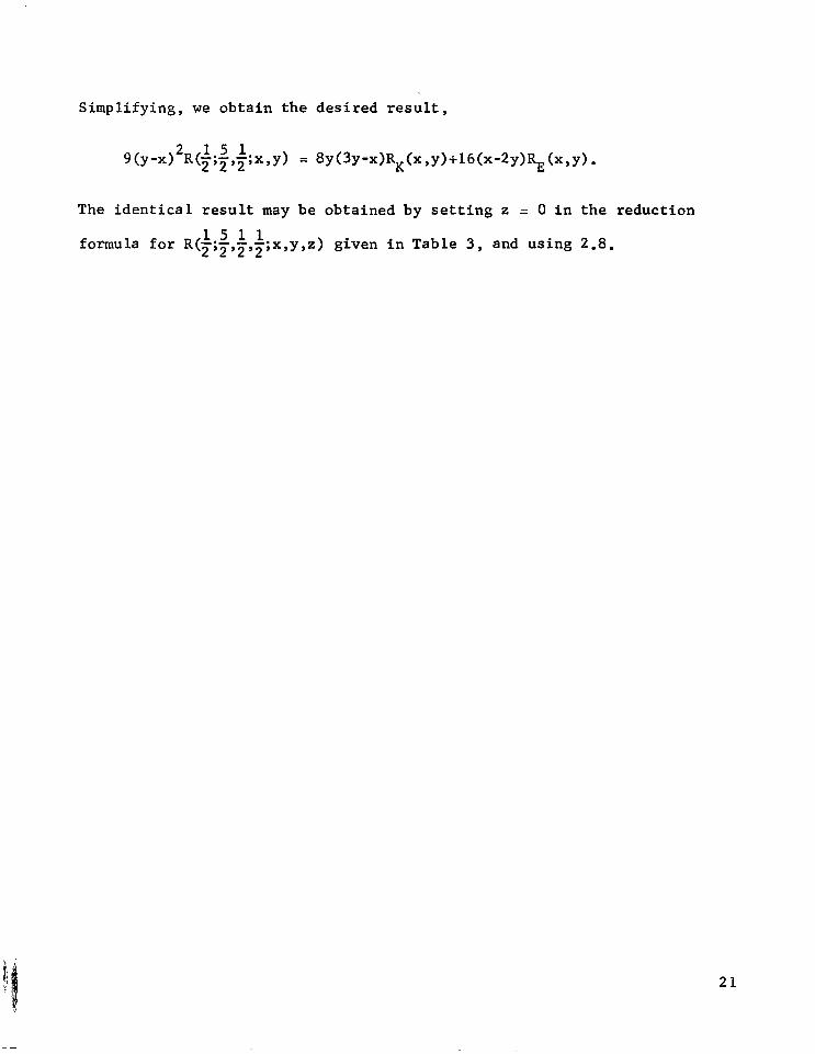
Simplifying, we obtain the desired result,
9(y-x)2R($$,+;x,y) = 8y(3y-x)s(x,y)+l6(x-2y)RE(x,y).
The identical result may be obtained by setting z = 0 in the reduction
1511 formula for R(F;T,~,~, -*x,y,z) given in Table 3, and using 2.8.
21
VII. TABLES
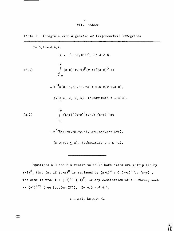
Table 1. Integrals with algebraic or trigonometric integrands
In 6.1 and 6.2,
a = -(c+Sv+&tl), Re a > 0.
(6.1)
X
s (z-t)a(w-t)P(v-t)Y(s-t)' dt
-03
=a -LR (a;-a,-p,-r,-6; z-x,w-x,v-x,s-x),
(x 5 2, w, v, s), (substitute t = x-u).
(6.2)
0.3
s (t-z)c(t-w)S(t-v)Y(t-s)' dt
X
= a-lR(a;-o, -p ,-y, -6; x-z ,x-w,x-v,x-s) ,
(z,w,v,s < x), (substitute t = x +u).
Equations 6.3 and 6.4 remain valid if both sides are multiplied by
(-9, that is, if (t-z)B is replaced by (z-t)' and (Y-z)~ by (z-y)".
The same is true for (-l)y, (-l)', or any combination of the three, such
as (-l)'? (see Section III). In 6.3 and 6.4,
a = c+l, Re a > -1.
22

Table 1. (Continued)
(6.3)
Y
J
(y-t)a(t-z)P(t-w)r(t-v)6 dt
X
.R(a;-P,-y,-6,~1,+p+y+6+2; ff$ , z , z, l),
(substitute t = (uy+x)(u+l)-1).
(6.4)
X
s (t-y)a(t-z)P(t-w)r(t-v)'dt
Y
-R(a;-p, -r, -6, a+p+r-+6+2 ; x-z x-w x-v l), y-z' y-w' y-v'
(substitute t = (uy+x)(u+l)-I).
0 (6.5) J (sin9)a(sin2$-sin 0) 2 P (c0s0)r(p+qcos2Q+rsin 6)) 2 'de
0
= i (p+q)S(sin$)a+2P+lB(q , p+l>
.R(+; 2, 1-r a+2B+y+28+2 2 cos2Q,p+qcos 2 4) +rsin 2 -8, ; p+q ? 11,
( 0 < 0 < f;Re a,Re p > -1), (substitute sin0 = (l+t) -l/2 sin@.
23
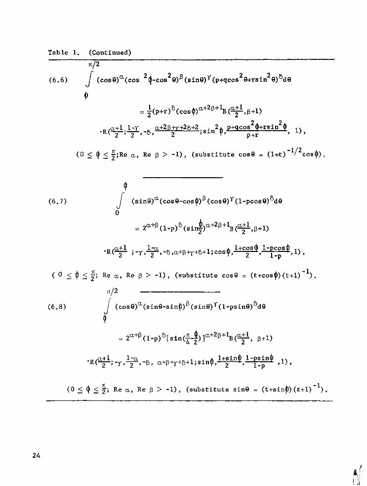
Table 1. (Continued)
d2 (6.6) J (cose)a(cos 20 2P -cos Q) (sinQ)r(p+qcos28+rsin2Q)'dQ
0
= $(p+r)S(c0s+)a+2P+$(+,pil)
a+2 +2&-t-2 ;sin2jI,P+q 2
.R(+;+ -6, *F cos +rsin2 p+r ? 11,
(0 5 0 < $;Re CI,, Re p > -l), (substitute case = (l+t) -l/2 cos$>.
(6.7) J (sine)a(cOse-cOs~)B(cOse)~(l-pcOse)~de
0
= 2a+B(1-p)6(si 2) A a+2p+l a+1 B( 2 -,P+l)
.R(L$L 1-u ; -r,-$f-’ -G,u+P+y+G+l;cos$, l-Pcoso, 1) lccos~
2 , Imp ,
(0 I$<;; Re a, Re p > -l), (substitute case = (t+cos$)(t+l)").
d2
(6.8) J (cosQ)"(sin&sin~)B(sin~)r(l-psinf3)'dQ
0
‘R(+; my,+,
(0 5 C/ 5 5; Re CL, Re p > -l), (substitute sine = (t+sinfQ(t+l)-1).
24

Table 2. Reduction formulas for complete integrals of the first and second kinds
These formulas are of the form
AR(a ;bl,b2;x,y) = AKRKSAERE,
where RK = R(+;$,$; X,Y) >
s = R(-$;;,+;x,y).
The symbol b is defined as
b = (bl,b2).
a a' !I A
5 1 2 2 3xy(x-y12 -16xy 8 (x+y>
2. 2 b-Yj2 g(x+y) -16 2 2
1 2
5 3(x-Y12 -16xy ~(x+Y) 2
(2 3) -1 7 2' 2
T F 15(x-y)2 -8xy(x+y) 16(x2+y2-xy)
E
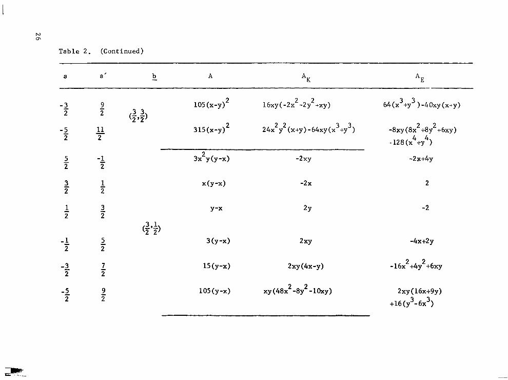
Table 2. (Continued)
a a' b A AK AE
-3 Ti-
-5 2
9 2
11 2
5 T
-1. 2
2 2
33 $q)
16xy(-2x2-2y2+xy)
24x2y2(x+y)-64xy(x3+y3)
3x2Y(Y-x)
X(Y-xl
-2xy
-2x
1 2 Y-x 2Y 2 2
(T'$ 31
-1 T
5 3(y-x) 2XY 2
-2 L 15(Y-x) ~xY(~x-Y) 2 2
-1. 9 105(y-x) xy(48x2-8y2-1Oxy) 2 2
64(x3+y3)-4Oxy(x;y)
-8xy(8x2i8y2+6xy)
+128(x4+y4)
-2x+4y
2
-2
-4x+2y
-16x2+4y2+6xy
2xy(16x+9y)
+16(y3-6x3)

Table 2. (Continued)
a a' ii! A AK AE
1 T
-1 2
-2 2
-5 2
5 2
2 2
1 2
-2 2
-1 2
3x3y -4xy -x+8y
2 X -X 2
X 0 1
3 -1 $9 g
1 'Y 2
3 -4xy 8x-y
15 xy(-24x+y) 48x2-2y2-8xy
3x2y2 'XY 11
CT q)
XY 0
2 (x+y >
1
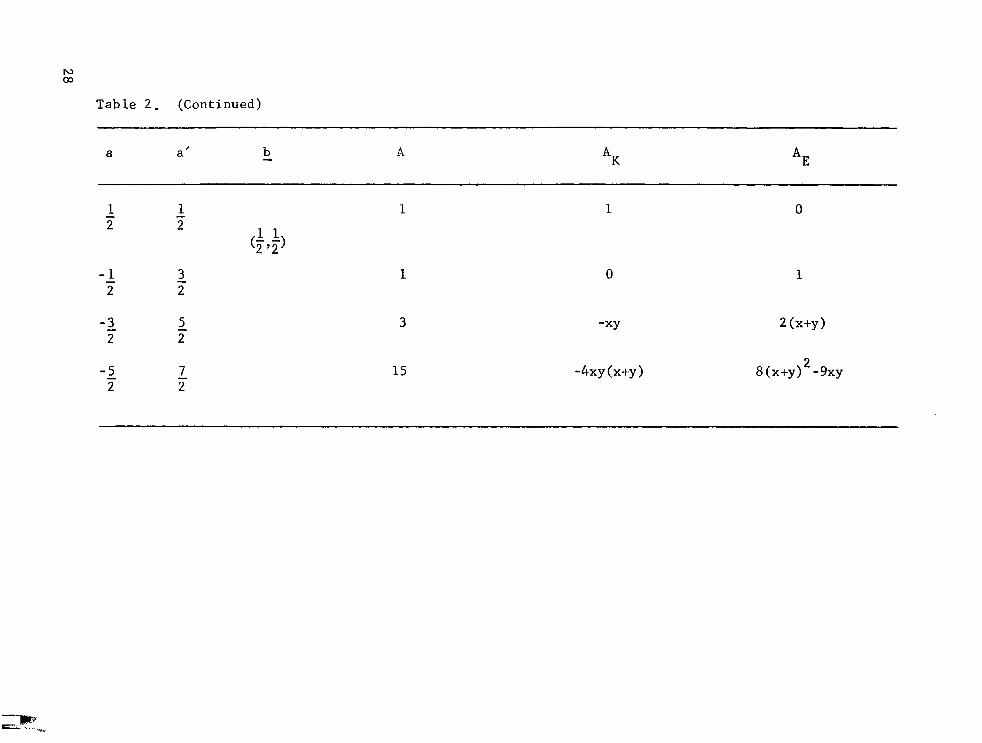
Table 2. (Continued)
b A AK AE
-1 2
-2 5 2 z
-5 2
1
1
3
15 -4xy(x+y) 8 (x+y>2 -9xy
1
0
‘XY
0
1
2 (x+y >

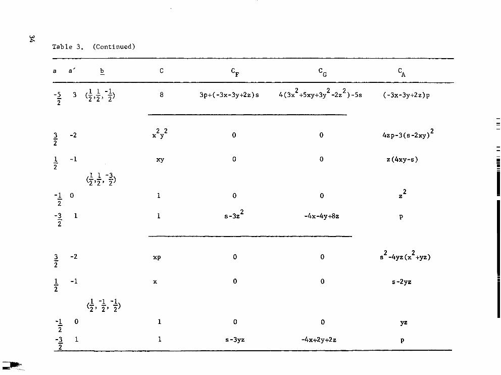
Table 3. Reduction formulas for incomplete integrals of the first and second kinds
These formulas are of the form
CR(a;bl,b2,b3;x,y,z) = CFRF + CGRG + CA(xyz) -l/2
,
where
RF = +$~,+,Y,~),
RG = R(-+;$$+;x,y,z),
(xyz) -v2 3111 = R(;?-;~T,T;x,Y 32).
The symbols s,p, and )- are defined as
s = xy+xz+yz
p = xyz
a = (bl,b2,b3)
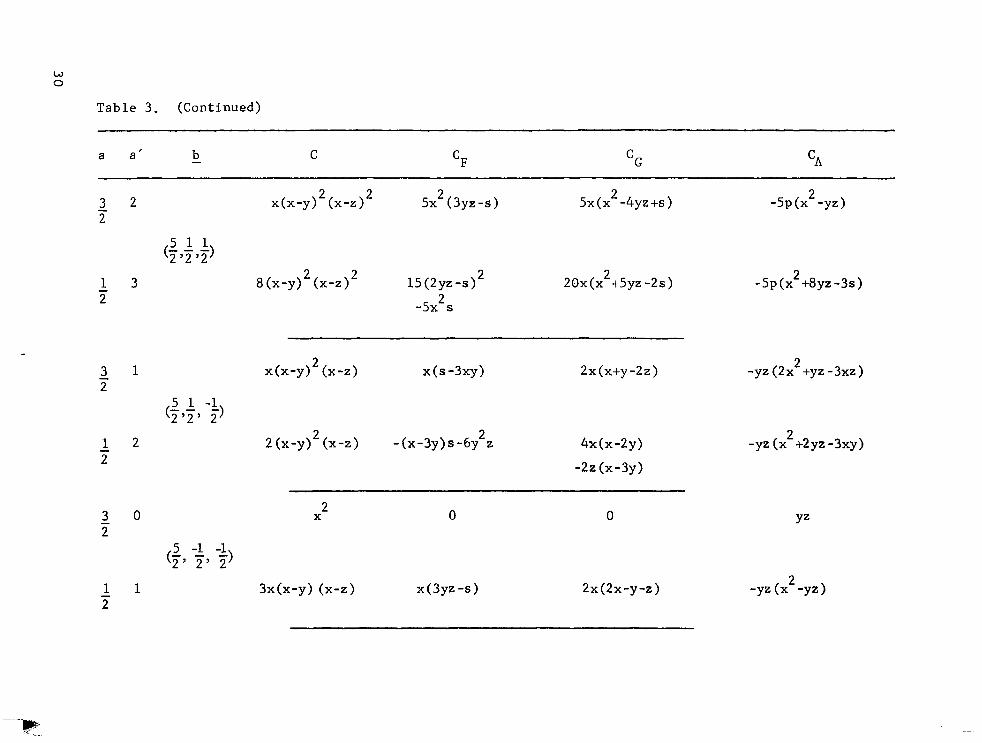
Table 3. (Continued)
a a' b C cF cG cA
2 2 x(x-y)2(x-z)2 5x2(3yz-s) 5x(x2 -4yz+s) -5p(x2-yz) 2
13 2
15(2yz-~)~
-5x2s
20x(x2+5yz-2s) -5p(x2+8yz-3s)
3 1 T
x(x-y>2 (x-z) x(s-3xy) 2x(x+y-2z)
$2' 5 1 -1 2)
12 2
2(x-y)2(x-z) -(x-3y)s-6y2z 4x(x-2y)
-22(x-3y)
2 0 2
1 1 2
2 X
3x(x-y)(x-z) x(3yz-s) 2x(2x-y-z)
-yz(2x2+yz-3xz)
-yz(x2+2yz-3xy)
YZ
-yz (x2-yz)

Table 3. (Continued)
a a’ b C cF cG cA
1 2
2 2
2 2
1 T
-1 T
-2 2
2 2
1 b
331 (pp$ ~(x-Y)~(Y-z)(x-z> 15z2 (x-y)2 3ox2(y-z) 15p(s-3xy)
+15xy(s-3xy) +30y2 (x-z)
3 3 -3 <py, 2) XY 0 0 2
Z
(x-y> (x-z > 3x -6 3YZ
2 (X-Y) (x-z > 3(2yz-s) 6x -3P
8 (X-Y) (x-z> 3x(2yz -s) 6(x-y) (x+)+6x2 -3xp
16(x-y) (x-z) -s [ (x-y) (x-z)+3x2 I
+6xp
(x-y) (x-z) (lox+4y+4z) -[ (x-y) (x-z)+3x2]p
+6x3
X 0 0
X-Y ‘Y 2
Z
-Y=
(21-l -1 2’2’ 2
L
I W I-

Table 3. (Continued)
a a' b C cF cG
-L 2 2
-3 3 2
2 -1 2
1 0 2
3 -1 2
1 0 2
-1 1 7
-2 2 2
2 0 2
(21 -1 2 2' 9
2 (x-y>
8(x-y)
2yz-s 4x-2y
-2 (4x-1-y) (x-y) 2 (x-y) (5x+2y-z)
-XY (4X-Y) +6x 2 -(4x-y)p
2 XY 0 0 3yz (z-x)+xz2
(,,p 3 1 -3 2)
2 X 0 0 z
2 X 0 0 4yz -s
X 0 0 Y= (,, 3 -1 -1
z, F> 1 -y-z 4 'Y=
1 3yz -2s 8x-y-z -2P
1 1 1 (2,py) 1 0 0 1
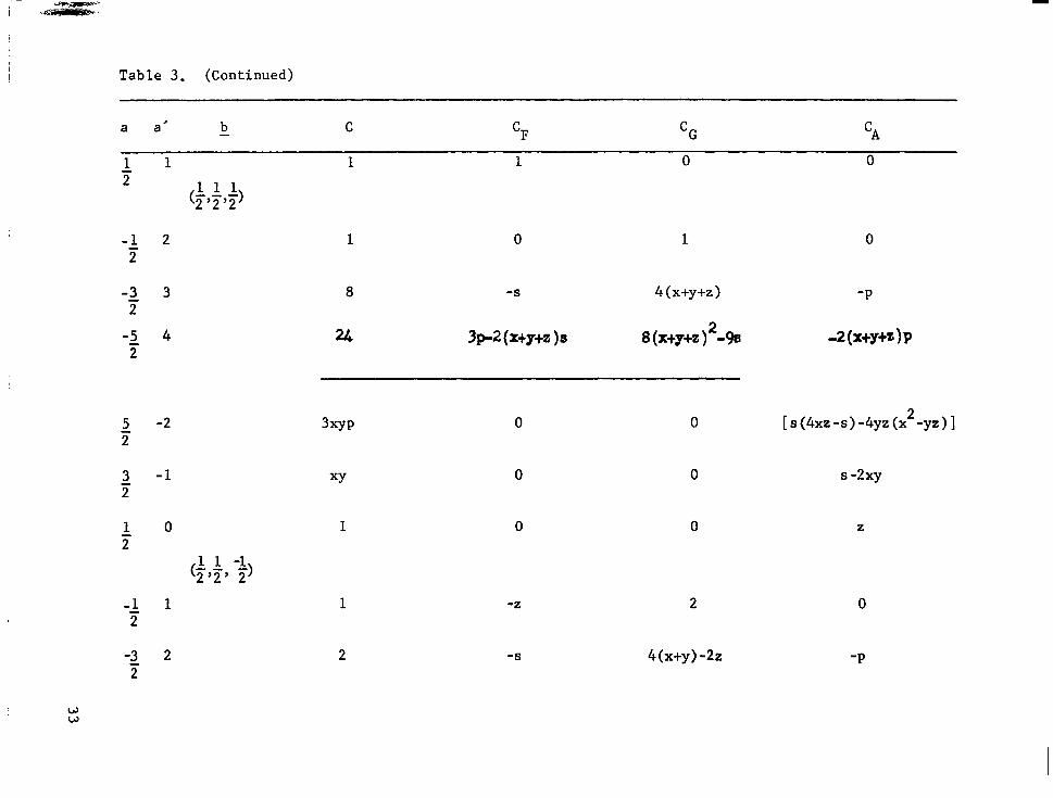
Table 3. (Continued)
a a' b C cF cG cA
1 1 2 111
(pp$
-1 2 2
-2 3 2
-5 4 2
2 -2 2
2 -1 2
10 Ti
<pp 1 1 -1 T>
-1 1 2
-2. 2 2
1 0 1
8 -S 4(x+y+z)
24 3~2 (xtytz )s 8(xtytz)2-9a
0
-P
-2(x+y+Qp
3XYP 0 0
XY 0 0
1 0 0
1 -2 2
2 -S 4(x+y) -22
[ s (4x2 ‘S) -4yz (x2 -yz) ]
s -2xy
z
0
-P
w w
W *
Table 3. (Continued)
a a' b C cF cG cA
-1 3 (;,+,-+) 8 3p+( -3x-3y+2z) s 4(3x2+5xy+3y2-2z2)-5s 2
(-3x-3y+2z)p
2 -2 2
1 -1 2
1 1 -3 (‘iq, F>
-1 0 2
-2 1 2
2 2 XY 0 0
XY 0 0
1 0 0
1 s-32 2 -4x-4y+8z
2 -2 2
1 -1 2
1 -1 -1 ('i-' 2, r>
-1 0 2
-3 1 7
XP
X
0 0
0 0
1 0 0 Y=
1 s -3yz -4x+2y+2z P
2 (4xy-s)
z2
P
s2 -4yz (x2+yz)
s -2yz
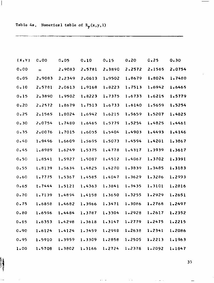
Table 4a. Numerical table of R+'Y, 1)
(X,Y) c.00 0.05 0.10 0.15 0.20 0.2s 0.30
0.00
0.05
0.10
0.15
0.20
0.25
0.30
0.35
0.40
0.45
0.50
0.55
0.60
0.65
0.70
0.75
0.80
0.85
0.90
0.95
1.00
co 2.9083 2.5781 2.3890 2.2572 2.1565 2.0754
2.9083 2.2349 2.0613 1.9502 1.8679 1.8024 1.7480
2.5781 2.0613 1.9168 1.8223 1.7513 1.6942 I.6465
2.3890 1.9502 1.8223 1.7375 1.6733 1.6215 1.5779
2.2572 1.8679 1.7513 1.6733 1.6140 1.5659 1.5254
2.1565 1.8024 1.6942 1.6215 l-5659 1.5207 1.4825
2.0754 1.7480 I.6465 1.5779 1.5254 1.4825 1.4461
2.0076 1.7015 1.6055 1.5404 1.4903 l-4493 1.4146
1.9496 1.6609 i.T695 1 .so73 1.4594 1.4201 1.3867
1.8989 1.6249 1.537s 1.4778 1.4317 1.3939 1.3617
1.8541 1.5927 1.5087 1.4512 1.4067 1.3702 1.3391
1.8139 1.5634 1.4825 1.4270 1.3839 I.3485 1.3183
1.777s 1.5367 1.4585 1.4047 1.3629 1.3286 1.2993
1.7444 1.5121 1.4363 1.3841 1.3435 1.3101 1.2816
1.7139 1.4894 1.4158 1.3650 1.3255 1.2929 1.2651
1.6858 1.4682 1.3966 1.3471 1.3086 1.2768 1.2497
1.6596 1.4484 1.3787 1.3304 1.2928 1.2617 1.2352
1.6353 1.4298 1.3618 1.3147 1.2779 1.2475 1.2215
1.6124 1.4124 1.3459 1.2998 1.2638 1.2341 1.2086
1.5910 1.3959 1.3309 1.2858 1.2505 1.2213 1.1963
1.5708 1.38C2 1.3166 1.2724 1.2378 1.2092 1.1847
35

Table 4a. (Continued)
(X*Y) 0.35 0.40 0.45 0.50 0.55 0.60 0.65
0.00 2.0076 1.9496 1.8989 1.8541 1.8139 1.7775 1.744.4
0.05 1.7015 1.6609 1.6249 1.5927 1.5634 1.5367 l-5121
0.10 1.6055 1.5695 1.5375 1.5087 1.4825 1.4585 1.4363
0.15 1.5404 1.5073 1.4778 1.4512 1.4270 1.4047 1.3841
0.20 1.4903 1.4594 1.4317 1.4C67 1.3839 1.3629 1.3435
0.25 1.4493 1.4201 1.3939 1.3702 1.3485 1.3286 1.3101
0.30 1.4146 1.3867 1.3617 1.3391 1.3183 1.2993 1.2816
0.35 1.3844 1.3577 1.3337 1.3119 1 l 2920 1.2736 1.2566
0.40 1.3577 1.3319 1.3088 1.2878 1.2686 1.2509 1.2344
0.45 1.3337 1.3088 1.2865 1.2662 1.2475 1.2304 1.2144
0.50 1.3119 1.2878 1.2662 1.2465 1.2284 1.2117 1.1962
0.55 1.2920 1.2686 1.2475 1.2284 1.2108 1.1946 1.1795
0.60 1.2736 1.2509 1.2304 1.2117 1.1946 1.1787 1.1640
0.65 1.2566 1.2344 1.2144 1.1962 1.1795 1.1640 1.1496
0.70 1.2407 1.2191 1.1995 1.1817 1.1654 1.1503 1.1362
0.7s 1.2259 1.2047 1.1856 1.1682 1.1522 1.1374 1.1236
0.80 1.2119 1.1912 1.1725 1.1554 1.1397 1.1252 1.. 1117
0.85 1.19e7 1.1784 1.1601 1.1433 1.1280 1.1137 1.100s
0.90 1.1862 1.1663 1.1483 1.1319 1.1168 1.1028 1.0898
0.95 1.1744 1.1548 1.1372 1.1211 1.1062 1.0925 1.0797
1.00 1.1631 1.1439 1.1266 1.1107 1.0961 1.0826 1.0701
36

Table 4a. (Continued)
(X,Y) 0.70 0.75 0.80 0.85 0.90 O.YS 1.00
0.00 1.7139 1.6858 1.6596
0.05 1.4894 1.4682 1.4484
0.10 1.4158 1.3966 1.3787
0.15 1.3650 1.3471 1.3304
0.20 1.3255 1.3086 1.2928
0.25 1.2929 1.2768 1.2617
0.30 1.2651 1.2497 1.2352
0.35 1.2407 1.2259 1.2119
0.40 1.2191 1.2047 1.1912
0.45 l-1995 1.1856 1.1725
0.50 1.1817 1.1682 1.1554
0.55 1.1654 1.1522 1.1397
0.60 1.1503 1.1374 1.1252
0.65 1.1362 1.1236 1.1117
0.70 1.1231 1.1107 1.0991
0.75 1.1107 1.0986 1.0872
0.80 1.0991 1.0872 1.0760
0.85 I.0881 1.0764 1.0654
0.90 1.0776 1.0662 1.0554
0.95 1.0677 1.0565 1.0459
1.00 1.0583 1.0472 1.0367
1.6353
1.4298
1.3618
1.3147
1.2779
1.2475
1.2215
1.1987
1.17E4
1.1601
1.1433
1.1280
1.1137
l.lOC5 .
1.0881
1.0764
1.0654
1.0550
1.0452
1.03S8
1.0269
1.6124 1.5910 1.5708
1.4124 1.3959 1.3802
1.3459 1.3309 1.3166
1.2998 1.2858 1.2724
1.2638 1.2505 1.2378
1.2341 1.2213 1.2092
1.2086 1.1963 1.1847
1.1862 1.1744 1.1631
1.1663 1.1548 1.1439
1.1483 1.1372 1.1266
1.1319 1.1211 1.1107
1.116R 1.1062 1.0961
L.1028 1.0925 1.0826
1.0898 1.0797 1.0701
1.0776 1.0677 1.0583
1.0662 1.0565 1.0472
1.0554 1.0459 1.0367
1.0452 1.0358 1.0269
1.0355 1.0263 1.0175
1.0263 1.0172 1.0085
1.0175 1.0085 1.0000
37

Table 4b. Numerical table of RG(x,y,l)
(X,Y) 0.00 0.05
0.00 0.5oco 0.5302
0.05 0.5302 0.5559
0.10 0.5524 0.5763
0.15 0.5717 0.5945
0.20 0.5892 0.6112
0.25 0.6055 0.6267
0.30 0.6208 0.6415
0.35 0.6354 0.6555
0.40 0.6452 0.6689
0.45 0.6625 0.6818
0.50 0.6753 0.6942
o.ss 0.6877 0.7063
0.60 0.6997 0.7180
0.65 0.7113 0.7294
0.70 0.7227 0.7404
0.75 0.7337 0.7513
0.80 0.7445 0.7618
0.85 0.7551 0.7721
0.90 0.7654 0.7823
0.95 0.7755 0.7922
1.00 0.7854 0.8019
38
0.10
0.5524
0.5763
0.5958
0.6133
0.6295
0.6446
0.6589
0.6726
0.6857
0.6983
0.7105
0.7223
0.7338
0.7450
0.7559
0.7665
0.7769
0.7871
0.7970
0.8068
0.8164
0.15 0.20 0.25 0.30
0.5717 0.5892 0.6055 0.6208
0.5945 0.6112 0.6267 0.6415
0.6133 0.6295 0.6446 0.6589
0.6303 0.6460 0.6608 0.6748
0.6460 0.6614 0.6759 0.6896
0.6608 0.6759 0.6901 0.7036
0.6748 0.6896 0.7036 0.7169
0.6882 0.7028 0.7166 0.7297
0.7011 0.7154 0.7290 0.7420
0.7135 0.7276 0.7410 0.7538
0.7254 0.7394 0.7527 0.7653
0.7371 0.7509 0.7640 0.7765
0.7484 0.7620 0.7750 0.7874
0.7594 0.7729 0.7857 0.7980
0.7701 0.7835 0.7962 0.8083
0.7806 0.7938 0.8064 0.8185
0.7908 0.8039 0.8164 0.8284
0.8009 0.8139 0.8262 0.8381
0.8107 0.8236 0.8359 0.8476
0.8204 0.8331 0.8453 0.8570
0.8299 0.8425 0.8546 0.8662
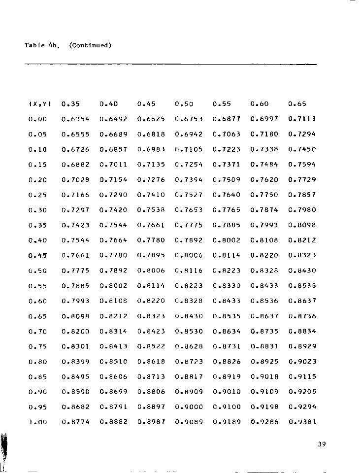
Table 4b. (Continued)
(X,Y) 0.35 0.40 0.45 0.50 0.55 0.60 0.65
0.00 0.6354 0.6492 0.6625 0.6753 0.6877 0.6997 0.7113
0.05 0.6555 0.6689 0.6818 0.6942 0.7063 0.7180 0.7294
0.10 0.6726 0.6857 0.6983 0.7105 0.7223 0.7338 0.7450
0.15 0.6882 0.7011 0.7135 0.7254 0.7371 0.7484 0.7594
0.20 0.7028 0.7154 0.7276 0.7394 0.7509 0.7620 0.7729
0.25 0.7166 0.7290 0.7410 0.7527 0.7640 0.7750 0.7857
0.30 0.7297 0.7420 0.7538 0.7653 0.7765 0.7874 0.7980
0.35 0.7423 0.7544 0.7661 0.7775 0.7885 0.7993 0.8098
0.40 0.7544 0.7664 0.7780 0.7892 0.8002 0.8108 cl.8212
OP45 0.7661 0.7780 0.7895 0.8006 0.8114 0.8220 0.8373
(1.50 0.7775 0.7892 0.8006 0.8116 0.8223 0.8328 0.8430
0.55 0.7885 0.8002 0.8114 0.8223 0.8330 0.8433 0.8535
0.60 0.7993 0.8108 0.8220 0.8328 0.8433 0.8536 0.8637
0.65 0.8098 0.8212 0.8323 0.8430 0.8535 0.8637 0.8736
0.70 0.8200 0.8314 0.8423 o.a530 0.8634 0.8735 0.8834
0.75 0.8301 0.8413 0.8522 0.8628 0.8731 0.8831 0.8929
0.80 0.R399 0.8510 0.8618 0.6723 0.8826 0.8925 0.9023
0.85 0.8495 0.8606 0.8713 0.8817 0.8919 0.9018 0.9115
0.90 0.8590 0.8699 0.8806 0.8909 0.9010 0.9109 0.9205
0.95 0.8682 0.8791 0.8897 0.9000 c.9100 0.9198 0.9294
1.00 0.8774 0.8882 0.8987 0.9089 0.9189 0.9286 0.9381
39

Table 4b. (Continued)
(X*Y) 0.70 0.75 0.80 0.85 0.90 c-95 1.00
0.00 0.7227 0.7337 0.7445 0.7551 0.7654 0.7755 0.7854
0.05 0.7404 0.7513 0.7618 0.7721 0.7823 0.7922 0.8019
0.10 0.7559 0.7665 0.7769 0.7871 0.7970 0.8068 0.8164
0.15 0.7701 0.7806 0.7908 0.8009 0.8107 0.8204 0.8299
0.20 0.7835 0.7938 0.8039 0.8139 0.8236 0.8331 0.8425
0.25 0.7962 0.8064 0.8164 0.8262 0.8354, 0.8453 0.8546
0.30 0.8083 0.8185 0.8284 0.8381 0.8476 c-8570 0.8662
0.35 0.8200 0.8301 0.8399 0.8495 o-as90 0.8682 0.8774
0.40 0.8314 0.8413 0.8510 0.8606 0.8699 0.8791 0.8882
0.45 0.8423 0.8522 0.8618 0.8713 0.8806 0.8897 0.8987
0.50 0.8530 0.8628 0.8723 0.8817 0.8909 0.9000 0.9089
0.55 0.8634 0.8731 0.8826 0.8919 0.9010 0.9100 0.9189
0.60 C-8735 0.8831 0.8925 0.9018 0.9109 0.9198 0.9286
0.65 0.8834 0.8929 C.9C23 0.9115 C-9205 0.9294 0.9381
0.70 0.8931 0.9026 0.9119 0.9210 0.9300 0.9388 0.9475
0.75 0.9026 0.9120 0.9212 c-9303 0.9392 0.9480 0.9566
0.80 0.9119 0.9212 0.9304 0.9394 0.9483 0.9570 0.9656
0.85 0.9210 0.9303 0.9394 0.9484 C-9572 0.9659 0.9744
0.90 0.9300 0.9392 0.9483 0.9572 0.9660 C-9746 0.9831
0.95 0.9388 0.9480 0.9570 0.9659 0.9746 0.9832 0.9916
1.00 0.9475 0.9566 0.9656 0.9744 0.9831 0.9916 1.0000
40

VIII. LITERATURE CITED
1. Carlson, B. C. Lauricella's hypergeometric function FD. Journal of
Mathematical Analysis and Applications 7: 452-470. 1963.
2. Carlson, B. C. Normal elliptic integrals of the first and second kinds. Duke Mathematical Journal 31: 405-419. 1964.
3. tiJyrd > P. F. and Friedman, M. D. Handbook of elliptic integrals for engineers and physicists. Berlin, Germany, Springer-Verlag. 1954.
4. Milne-Thomson, L. M. Elliptic integrals. In Abramowitz, Milton and Stegun, Irene, eds. Handbook of mathematical functions. pp. 587-626. Washington, D. C., IJ. S. Government Printing Office. 1964.
5. Griibner, Wolfgang and Hofreiter, Nikolaus. Integraltafel. Parts 1 and 2. Vienna, Austria, Springer-Verlag. 1957 and 1958.
rs . Carlson, B. C. On computing elliptic integrals and functions. To be published in Journal of Mathematics and Physics. circa July, 1965.
41
IX. ACKNOWLEDGEMENTS
The author wishes to express his sincere gratitude to Dr. B. C.
Carlson for both his professional and personal advice and encouragement.
The author also wishes to thank two members of the Ames Laboratory Computer
Service Group, Mr. James Delany and Mr. Frank Carlsen. Mr. Delany wrote
the Fortran subroutine program to calculate RR and RG using quadratic
transformations. Mr. Carlsen provided valuable advice for the computation
of R F and R G directly from their power series expansions.
42

X. APPENDIX: FORTRAN SUBROUTINE PROGRAM FOR
COMPUTING RF AND RG BY MEANS OF DESCENDING
GAUSS OR ASCENDING IANDEN TRANSFORMATIONS
This program has been written under the assumption that
05x5 ysz. Particular values worthy of note are RF (O,O,l) =
m and RG(O,O,l) = l/2.
5 8
10
11 9
12
13
14
15
21
80
SUBROUTINE ELINT(X,Y,Z,RF,RG,INF) DIMENSION V(3),W(3)
IF(X) 7,8,8 SQRTZ =SQRTF(Z) IF(Y) 7,10,11 INF=l RG=.5":SQRTZ GOT0 7 INF=O IF(Z-X) 13,12,13 RF=~./SQRTZ RG-SQRTZ GOT0 7 D=Y+Y-X-Z A=SQRTF(Z-X) IF(D) 15,14,14 T=SQRTZ H=SQRTF(X) cszz-Y GOT0 21 T=SQRTF(X) H=SQRTZ CS=Y-x T=.5+c(T+SQRTF(Y)) N=O A=.5yc(A+SQRTF(A;'rA-CS)) CC=(.25+CS)/A cs =ccxc N=N+l V(N)=A;';A-CS W(N)=H IF(N-1) 81,82,81
43

82
17
18 19
20 81 23 24
25 26
27 28
29
30
33
32
31 34
35 36
7
E&C/A IF(E-7.46E-3) 18,18,17 NMAX-3 GOT0 81 IF(E-1.39E-5) 20,20,19 NMAXZ2 GOT0 81 NMfiX=l IF@-N-Mix) 23,27,23 IF(D) 25,24,24 Q=SQRTF(T>kT-CS) GOT0 26 Q=SQRTF(T*T+CS) H-(WAT)/Q T=.S"(T+O) GOT0 80 IF(D) 29,28,28 RF=(ASINF(A/T))/A GOT0 30 AT&/T RF=(LOGF(AT+SQRTF(l.tATJcAT)))/A B=V(l) CL-W(l) IF(NMAX-2) 31,32,33 B&d.f~(V(3)-V(2)) cLc+4*qw(3)-w(2)) V21=V(2)-V(1) W21=W(2)-W(1) Bd3+V21+V21 C&lW21+W21 IF(D) 34,35,35 UL;z-B COT0 36 U=X+B RGz,5f:(IJ~:-RFcC) RETURN END
44 NASA-Langley, 1965 CR-289

“The aeronautical and space activities of the United States shall be conducted so as to contribute . . . to the expansion of human knowl- edge of phenomena in the atmosphere and space. The Administration shall provide for the widest practicable and appropriate dissemination of information concerning its actiuities and the results thereof."
-NATIONAL AERONAUTICS AND SPACE ACT OF 1958
NASA SCIENTIFIC AND TECHNICAL PUBLICATIONS
TECHNICAL REPORTS: Scientific and technical information considered important, complete, and a lasting contribution to existing knowledge.
TECHNICAL NOTES: Information less broad in scope but nevertheless of importance as a contribution to existing knowledge.
TECHNICAL MEMORANDUMS: Information receiving limited distri- bution because of preliminary data, security classification, or other reasons.
CONTRACTOR REPORTS: Technical information generated in con- nection with a NASA contract or grant and released under NASA auspices.
TECHNICAL TRANSLATIONS: Information published in a foreign language considered to merit NASA distribution in English.
TECHNICAL REPRINTS: Information derived from NASA activities and initially published in the form of journal articles.
SPECIAL PUBLICATIONS: Information derived from or of value to NASA activities but not necessarily reporting the results ,of individual NASA-programmed scientific efforts. Publications include conference proceedings, monographs, data compilations, handbooks, sourcebooks, and special bibliographies.
Details on the availability of these publications may be obtained from:
SCIENTIFIC AND TECHNICAL INFORMATION DIVISION
NATIONAL AERONAUTICS AND SPACE ADMINISTRATION
Washington, D.C. PO546