Embed Size (px)
Citation preview

arX
iv:m
ath/
0701
436v
2 [
mat
h.C
A]
8 A
ug 2
007
GENERALIZED ELLIPTIC INTEGRALS
Ville Heikkala†,Mavina K. Vamanamurthy,
and
Matti Vuorinen
File: ggem74.tex, printed: 2008-2-2, 11.56
Abstract
Jacobi’s elliptic integrals and elliptic functions arise naturally from the Schwarz-Christoffel conformal transformation of the upper half plane onto a rectangle. Inthis paper we study generalized elliptic integrals which arise from the analogousmapping of the upper half plane onto a quadrilateral and obtain sharp mono-tonicity and convexity properties for certain combinations of these integrals, thusgeneralizing analogous well-known results for classical conformal capacity and qua-siconformal distortion functions. An algorithm for the computation of the modulusof the quadrilateral is given.
2000 Mathematics Subject Classification: Primary 33B15, 33C05, Secondary30C62.
1 Introduction
Given complex numbers a, b, and c with c 6= 0,−1,−2, . . ., the Gaussian hypergeometricfunction is the analytic continuation to the slit plane C \ [1,∞) of the series
F (a, b; c; z) = 2F1(a, b; c; z) =
∞∑
n=0
(a, n)(b, n)
(c, n)
zn
n!, |z| < 1 .(1.1)
Here (a, 0) = 1 for a 6= 0, and (a, n) is the shifted factorial function or the Appell symbol
(a, n) = a(a + 1)(a + 2) · · · (a + n − 1)
for n ∈ N \ {0}, where N = {0, 1, 2, . . .}.†Author supported by the Magnus Ehrnrooth fund of the Finnish Academy of Science and Letters.
1

A generalized modular equation of order (or degree) p > 0 is
F (a, b; c; 1 − s2)
F (a, b; c; s2)= p
F (a, b; c; 1 − r2)
F (a, b; c; r2), 0 < r < 1 .(1.2)
Sometimes we just call this an (a, b, c)-modular equation of order p and we usually assumethat a, b, c > 0 with a + b ≥ c, in which case this equation uniquely defines s, see Lemma4.5.
Many particular cases of (1.2) have been studied in the literature on both analyticnumber theory and geometric function theory, [Be], [BB], [BBG], [AVV], [AQVV], [LV].The classical case (a, b, c) = (1
2, 1
2, 1) was studied already by Jacobi and many others in the
nineteenth century, see [Be]. In 1995 B. Berndt, S. Bhargava, and F. Garvan publishedan important paper [BBG] in which they studied the case (a, b, c) = (a, 1 − a, 1) andp an integer. For several rational values of a such as a = 1
3, 1
4, 1
6and integers p (e.g.
p = 2, 3, 5, 7, 11, ...) they were able to give proofs for numerous algebraic identities statedby Ramanujan in his unpublished notebooks. These identities involve r and s from (1.2).After the publication of [BBG] many papers have appeared on modular equations, seee.g. [AQVV], [Be], [CLT], [Q], and [S].
To rewrite (1.2) in a slightly shorter form, we use the decreasing homeomorphismµa,b,c : (0, 1) → (0,∞), defined by
µa,b,c(r) =B(a, b)
2
F (a, b; c; r′2)
F (a, b; c; r2), r ∈ (0, 1)(1.3)
for a, b, c > 0, a + b ≥ c, where B is the beta function, see (3.5) below. We call µa,b,c thegeneralized modulus, cf. [LV, (2.2)]. We can now write (1.2) as
µa,b,c(s) = pµa,b,c(r) , 0 < r < 1 .(1.4)
With p = 1/K, K > 0, the solution of (1.2) is then given by
s = ϕa,b,cK (r) = µ−1
a,b,c(µa,b,c(r)/K) .(1.5)
We call ϕa,b,cK the (a, b, c)-modular function with degree p = 1/K [BBG], [AQVV, (1.5)].
In the case a < c we also use the notation
µa,c = µa,c−a,c , ϕa,cK = ϕa,c−a,c
K .
For 0 < a < min{c, 1} and 0 < b < c ≤ a + b, define the generalized complete ellipticintegrals of the first and second kinds (cf. [AQVV, (1.9), (1.10), (1.3), and (1.5)]) on [0, 1]by
K = Ka,b,c = Ka,b,c(r) =B(a, b)
2F (a, b; c; r2) ,(1.6)
E = Ea,b,c = Ea,b,c(r) =B(a, b)
2F (a − 1, b; c; r2) ,(1.7)
K′ = K
′
a,b,c = Ka,b,c(r′) , and E
′ = E′
a,b,c = Ea,b,c(r′)(1.8)
2

for r ∈ (0, 1), r′ =√
1 − r2. The end values are defined by limits as r tends to 0+ and1−, respectively. In particular, we denote Ka,c = Ka,c−a,c and Ea,c = Ea,c−a,c . Thus, by(3.9) below,
Ka,b,c(0) = Ea,b,c(0) =B(a, b)
2
and
Ea,b,c(1) =1
2
B(a, b)B(c, c + 1 − a − b)
B(c + 1 − a, c − b), Ka,b,c(1) = ∞ .
Note that the restrictions on a, b and c ensure that the function Ka,b,c is increasing andunbounded whereas Ea,b,c is decreasing and bounded, as in the classical case a = b =12, c = 1. Note also that our terminology differs from that of [BB, Section 5.5], where
generalized elliptic integrals refer to the particular case c = 1.In this paper we study the modular function ϕa,b,c
K and the generalized modulus µa,b,c
as well as the generalized elliptic integrals Ka,b,c and Ea,b,c. In the case b = 1 − a, c = 1,these functions coincide with the special cases ϕa
K , µa, Ka, and Ea which were studied in[AQVV].
In Section 2 we construct a conformal mapping from a quadrilateral with internalangles bπ, (c − b)π, (1 − a)π, and (1 − c + a)π onto the upper half plane. We denotethis mapping by sna,b,c. If b = 1 − a and c = 1, this mapping reduces to the generalizedelliptic sine function sna in [AQVV, 2.1]. We given an algorithm for the computation of
the conformal modulus of a quadrilateral and its implementation in the Mathematicar
language. In a later work, we study the dependence of the modulus on the geometry ofthe quadrilateral, [DV], [RV].
In Section 3 we recall some basic properties of the hypergeometric, gamma, and betafunctions, that are used in the sequel.
Section 4 contains our main results: differentiation formulas and monotone proper-ties of the generalized elliptic integrals and of several combinations of these functions.Theorems 4.3 and 4.4, which provide sufficient conditions for the quotients of two Maclau-rin series to be monotone increasing, seem to be of independent interest and, as far aswe know, these results are new. Also a similar result is given for the quotient of twopolynomials of the same degree.
The special functions Ka,b,c, µa,b,c and quotients of hypergeometric functions are presentlystudied very intensively. The manuscript [HLVV] is a direct continuation of this workand for some particular parameter triples (a, b, c) there are very recent results by manyauthors [B1]-[B4], [KS], [WZQC], [ZWC].
Throughout this paper we denote r′ =√
1 − r2 whenever r ∈ (0, 1). The standardsymbols C, R, Z, and N denote the sets of complex numbers, real numbers, integers, andnatural numbers (with zero included), respectively.
2 The Schwarz-Christoffel map onto a quadrilateral
For 0 < a, b < 1, max{a + b, 1} ≤ c ≤ min{a, b} + 1, r ∈ (0, 1), let gr(t) = tb−1(1 −t)c−b−1(1 − r2t)−a, t ∈ C, Im t ≥ 0, denote the analytic branch for which the argumentof each of the factors t, 1 − t, and 1 − r2t is π whenever it is real and negative. Denote
3

C = C(b, c) = 1/B(b, c − b). We define the generalized Jacobi sine function sna,b,c(w) =sna,b,c(w, r) as the inverse of the function f given on the closed upper half plane by
w = f(z) = fa,b,c(z) = C
∫ z
0
gr(t)dt
= C
∫ z
0
tb−1(1 − t)c−b−1(1 − r2t)−adt(2.1)
= ei(a+b+1−c)πCr−2a
∫ z
0
tb−1(t − 1)c−b−1(t − 1/r2)(1−a)−1dt .
Recall the Euler integral representation [AAR, Theorem 2.2.1] [AS, 15.3.1]
F (a, b; c; z) =Γ(c)
Γ(b)Γ(c − b)
∫ 1
0
tb−1(1 − t)c−b−1(1 − tz)−adt(2.2)
= C(b, c)ei(a+b+1−c)π
∫ 1
0
tb−1(t − 1)c−b−1(tz − 1)−adt
for Re c > Re b > 0 and z ∈ C \ {u ∈ R | u ≥ 1}.The next result is well-known, but for the sake of completeness a proof is given.
As general references concerning the Schwarz-Christoffel mapping [M] and [N] may bementioned.
2.3. Proposition. The Schwarz-Christoffel mapping of the upper half plane H ontoa quadrilateral with turning angles βkπ at the vertices ak ∈ R is
w = F (z) =
∫ z
0
dz
Π4k=1(z − ak)βk
, −1 < βk < 1,
4∑
k=1
βk = 2,
where ak are the points on the real axis that F maps to the four vertices of the quadrilat-eral.
Proof. As in [N, pp. 192-193] let T : H → U be the Mobius transformation T (z) =(z − i)/(z + i) , where U is the unit disk {z : |z| < 1}. Then f(z) = F (T−1(z)) maps Uonto the quadrilateral Q and
f(ζ) =
∫ ζ
0
dw
Π4k=1(w − ζk)βk
,
where ζk are the points on the unit circle that map onto the four vertices of the quadri-lateral Q. Now
ζf ′′(ζ)
f ′(ζ)= −
4∑
k=1
βkζ
(ζ − ζk)=
4∑
k=1
βk1 + ζkζ
1 − ζkζ
and recalling that the βk sum to 2 we have that
1 +ζf ′′(ζ)
f ′(ζ)=
1
2
4∑
k=1
βk1 + ζkζ
1 − ζkζ.
4

For all points ζ ∈ U
Re
{
1 +ζf ′′(ζ)
f ′(ζ)
}
=1
2
4∑
k=1
βkRe
{
1 + ζkζ
1 − ζkζ
}
=1
2
4∑
k=1
βk1 − |ζ |2|1 − ζkζ |2
> 0 .
This proves that f maps U bijectively onto a convex domain, since Re {1+ζf ′′(ζ)/f ′(ζ)} >0 is a necessary and sufficient condition for this to be true, see [N, Ex. 5, p. 224]. �
1 2
1
2
3
4
m = 0.02+0.02i p = 2+0.02i
q = 2+4is = 0.02+4i
0.2 0.4 0.6 0.8 1 1.2
0.25
0.5
0.75
1
1.25
1.5
1.75
f(0)
f(1)
f(1/r^2)
f(Infinity)
f(m)
f(p)
f(q)f(s)
Figure 1: The image quadrilateral and the image of a grid under the mapping fa,b,c witha = 0.2, b = 0.3, c = 1.0, r = 0.7
2.4. Theorem. Let H denote the closed upper half-plane {z ∈ C | Im z ≥ 0} and let0 < a, b < 1, max{a + b, 1} ≤ c ≤ 1 + min{a, b}, r ∈ (0, 1). Then the function f in (2.1)is a homeomorphism of H onto the quadrilateral Q with vertices
f(0) = 0 , f(1) = F (a, b; c; r2) ,
f(1/r2) = f(1) +B(c − b, 1 − a)
B(b, c − b)e(b+1−c)iπr′
2(c−a−b)F (c − a, c − b; c + 1 − a − b; r′
2) ,
and
f(∞) = f(1/r2) +B(1 − a, a + 1 − c)
B(b, c − b)ei(a+b+1−c)πr2(1−c)r′
2(c−a−b)F (1− b, 1− a; 2− c; r2) ,
and interior angles bπ, (c− b)π, (1− a)π and (a + 1− c)π, respectively, at these vertices.It is conformal in the interior of H.
5

Proof. It is clear that f(0) = 0 and by (2.2) f(1) = F (a, b; c; r2). Next we evaluate
f(1/r2) = C
∫ 1/r2
0
gr(t)dt
= C
∫ 1
0
gr(t)dt + C
∫ 1/r2
1
gr(t)dt
= F (a, b; c; r2) + C
∫ 1/r2
1
gr(t)dt .
To evaluate the second integral above, we make the change of variable t = 1/(1 − r′2u)for which dt = (1 − r′2u)−2r′2du. We observe that this change of variable is simply therestriction to reals of the plane Mobius transformation taking the ordered triple (1, 1/r2, 0)onto the ordered triple (0, 1,∞). Then
gr(t)dt = (1 − r′2u)1−b
(
1 − 1
1 − r′2u
)c−b−1(
1 − r2
1 − r′2u
)
−a
(1 − r′2u)−2r′
2du
= (−1)b+1−cr′2(c−a−b)
uc−b−1(1 − u)−a(1 − r′2u)a−cdu
= e(b+1−c)iπr′2(c−a−b)
uc−b−1(1 − u)−a(1 − r′2u)a−cdu
and by (2.2) we get
C
∫ 1/r2
1
gr(t)dt = e(b+1−c)iπr′2(c−a−b) Γ(c)
Γ(b)Γ(c − b)
∫ 1
0
uc−b−1(1 − u)−a(1 − r′2u)a−cdu
= e(b+1−c)iπr′2(c−a−b) Γ(c)
Γ(b)Γ(c − b)
Γ(c − b)Γ(1 − a)
Γ(c + 1 − a − b)·
·F (c − a, c − b; c + 1 − a − b; r′2)
=B(c − b, 1 − a)
B(b, c − b)e(b+1−c)iπr′
2(c−a−b)F (c − a, c − b; c + 1 − a − b; r′
2)
=B(c − b, 1 − a)
B(b, c − b)e(b+1−c)iπr2(1−c)r′
2(c−a−b) ·
·F (1 − a, 1 − b; c + 1 − a − b; r′2) ,
where the last expression follows from (3.9) below. Hence f(1/r2) has the value claimed.We proceed to evaluate the remaining value, namely
f(∞) = C
∫
∞
0
gr(t)dt = C
∫ 1/r2
0
gr(t)dt + C
∫
∞
1/r2
gr(t)dt .
The first integral above equals f(1/r2). To compute the second one, we apply the changeof variable t = (1 − r2v)/(r2(1 − v)). We observe that this change of variable is simplythe restriction to reals of the plane Mobius transformation taking the ordered triple(1/r2,∞, 1) onto the ordered triple (0, 1,∞). Then dt = (1− r2)/(r2(1−v)2)dv, t = 1/r2
gives v = 0, and t = ∞ gives v = 1. We get
gr(t)dt =
(
1 − r2v
r2(1 − v)
)b−1(
1 − 1 − r2v
r2(1 − v)
)c−b−1
·
6

·(
1 − r2(1 − r2v)
r2(1 − v)
)
−a(1 − r2
r2(1 − v)2
)
dv
= r2(1+a−b+b+1)(1 − v)a−c(1 − r2v)b−1(r2 − 1)c−b−1(r2(r2 − 1)v)−a(1 − r2)dv
= (−1)a+b+1−cr′2(c−a−b)
r2(1−c)v−a(1 − v)a−c(1 − r2v)b−1dv
so that
C
∫
∞
1/r2
gr(t)dt = (−1)a+b+1−cr′2(c−a−b)
r2(1−c)C
∫ 1
0
v−a(1 − v)a−c(1 − r2v)b−1dv
= (−1)a+b+1−cr′2(c−a−b)
r2(1−c) B(1 − a, 1 + a − c)
B(b, c − b)·
·F (1 − b, 1 − a; 2 − c; r2) .
The claimed value for f(∞) follows.It follows from the formula (2.1) that (see e.g. [M, pp. 128–134]) f is a Schwarz-
Christoffel transformation which maps H onto a quadrilateral Q with vertices f(0), f(1),f(1/r2), and f(∞) and interior angles bπ, (c − b)π, (1 − a)π, and (1 − c + a)π in coun-terclockwise order. By Proposition 2.3 f is univalent. �
2.5. Corollary. Let 0 < a, b < 1, max{a + b, 1} ≤ c ≤ 1 + min{a, b}, and let Qbe a quadrilateral in the upper half plane with vertices 0, 1, A and B, the interior anglesat which are, respectively, bπ, (c − b)π, (1 − a)π and (1 + a − c)π. Then the conformalmodulus of Q (cf. [LV]) is given by
mod(Q) = K(r′)/K(r),
where r ∈ (0, 1) satisfies the equation
A − 1 =Lr′2(c−a−b)F (c − a, c − b; c + 1 − a − b; r′2)
F (a, b; c; r2)= G(r) ,(2.6)
say, and
L =B(c − b, 1 − a)
B(b, c − b)e(b+1−c)iπ.
Proof. Clearly, arg(A−1) = (b+1− c)π = arg(L). Since G(0) = ∞ and G(1) = 0,it follows that a unique solution r ∈ (0, 1) of equation (2.6) exists. Let f be as inTheorem 2.4 and let g = f/f(1). Then g maps the upper half plane H onto Q, withg(0) = 0, g(1) = 1, g(1/r2) = A, and g(∞) = B. The function h = sn−1 maps the firstquadrant conformally [Bo] onto the standard rectangle R, with h(0) = 0, h(1) = K(r),h(1/r) = K(r) + iK(r′), and h(∞) = iK(r′). Hence the function k = h(
√) maps H
conformally onto R. Thus, by conformal invariance, mod(Q) = K(r′)/K(r). �
2.7. Remark. (1) The quadrilateral Q in Theorem 2.4 reduces to a trapezoid if andonly if c = 1 or c = a + b, to a parallelogram if and only if c = 1 = a + b, [AQVV] and toa rectangle (the classical case) if and only if a = b = 1
2and c = 1, [Bo].
(2) The hypotheses in Corollary 2.5 imposed on the triple a, b, c imply that the quadri-lateral Q is convex.
7

2.8. Remark. Bowman [Bo, pp. 103-104] gives a formula for the conformal modulusof the quadrilateral with vertices 0, 1, 1+hi, and (h− 1)i when h > 1 as q = K(r)/K(r′)where
r =
(
t1 − t2t1 + t2
)2
, t1 = µ−1( π
2c
)
, t2 = µ−1(πc
2
)
, c = 2h − 1 .
Therefore, the quadrilateral can be conformally mapped onto the rectangle 0, 1, 1 + qi,qi with vertices corresponding.
2.9. Computational discovery. We have written a Mathematicar function thatcomputes the modulus of the quadrilateral with vertices at 0, 1, A, B where Im A >0, Im B > 0. This led to the following discovery for symmetric quadrilaterals:
If |B| = 1 and 2argA = argB, then the modulus is equal to 1 .(2.10)
It is not difficult to prove this analytically (see e.g. [Hen, p. 433] or [Her]). The followingfigure illuminates the variation of the modulus of the quadrilateral with vertices 0, 1, x +iy, i in the first quadrant.
1
2
3
4
x
1
23
4y
0
0.5
1
1.5
2
Mod
1
2
3x
1
23
y
Figure 2: Modulus of the quadrilateral with vertices 0, 1, x + iy, i and the line (x, x, 1).
2.11. Duplication formula for quadrilateral modulus. For the sake of convenientnotation, denote by QM(a, b, c, d) the modulus of the polygon with vertices a, b, c, d. Thatis, QM(a, b, c, d) = q if and only if there exists a conformal map of the polygon onto therectangle with vertices 1 + iq, iq, 0, 1 such that the vertices correspond. Clearly QM(1 +iq, iq, 0, 1) = q. Remark 2.8 gives now an explicit formula for QM(1 + ih, i(h − 1), 0, 1)
8
when h > 1. (By the way, it seems likely that QM(1 + ih, i(h − 1), 0, 1) ∈ [h − 1, h].) By(2.10) we see that QM(teiπ/4, i, 0, 1) = 1 for all t > 0 and it is clear by symmetry that
QM(tei(π/4−α), i, 0, 1) = 1/QM(tei(π/4+α), i, 0, 1)
for all α ∈ (0, π/4) and all t > 0. From [AQVV, Corollary 2.3] we have an expression forthe parallelogram case QM(1 + reiα, reiα, 0, 1).
We are not familiar with cases other than those mentioned above where the values ofQM(a, b, c, d) could be expressed in reasonably simple form. Therefore it might be of someinterest to record a duplication formula for QM(a, b, c, d) which follows from an elementarysymmetry consideration. To this end, let h, k > 0 and consider the quadrilaterals (1 +ih, ik,−ik, 1 − ih) and (1 + ih, ik, 0, 1). It is clear by symmetry that
QM(1 + ih, ik,−ik, 1 − ih) = 2QM(1 + ih, ik, 0, 1) .
We now use the invariance of QM(a, b, c, d) under homotheties to express this result in asimpler form. Choose a homothety T (z) = az + b with T (−ik) = 0, T (1− ih) = 1. Thena = 1/c, b = ik/c with c = 1 + i(k − h). Because
T (1 + ih) = (1 + i(h + k))/c , T (ik) = 2ik/c , T (−ik) = 0 , and T (1 − ih) = 1 ,
we have for h, k > 0, c = 1 + i(k − h) that
QM((1 + i(h + k))/c, 2ik/c, 0, 1) = 2QM(1 + ih, ik, 0, 1) .(2.12)
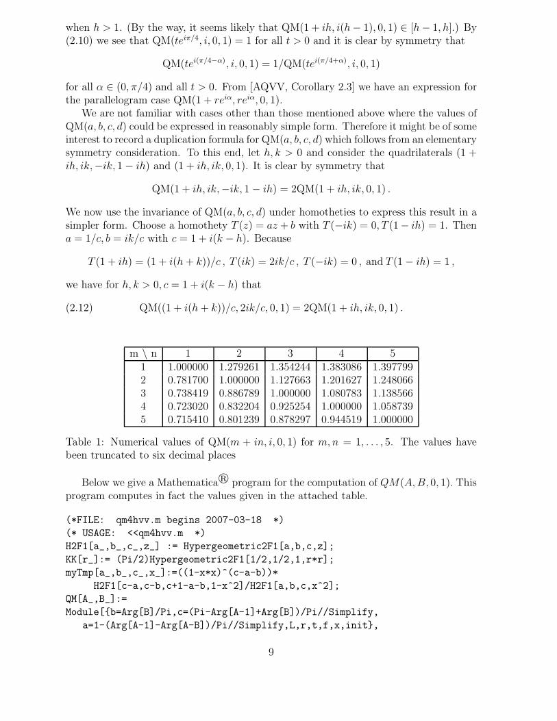
m \ n 1 2 3 4 51 1.000000 1.279261 1.354244 1.383086 1.3977992 0.781700 1.000000 1.127663 1.201627 1.2480663 0.738419 0.886789 1.000000 1.080783 1.1385664 0.723020 0.832204 0.925254 1.000000 1.0587395 0.715410 0.801239 0.878297 0.944519 1.000000
Table 1: Numerical values of QM(m + in, i, 0, 1) for m, n = 1, . . . , 5. The values havebeen truncated to six decimal places
Below we give a Mathematicar program for the computation of QM(A, B, 0, 1). Thisprogram computes in fact the values given in the attached table.
(*FILE: qm4hvv.m begins 2007-03-18 *)
(* USAGE: <<qm4hvv.m *)
H2F1[a_,b_,c_,z_] := Hypergeometric2F1[a,b,c,z];
KK[r_]:= (Pi/2)Hypergeometric2F1[1/2,1/2,1,r*r];
myTmp[a_,b_,c_,x_]:=((1-x*x)^(c-a-b))*
H2F1[c-a,c-b,c+1-a-b,1-x^2]/H2F1[a,b,c,x^2];
QM[A_,B_]:=
Module[{b=Arg[B]/Pi,c=(Pi-Arg[A-1]+Arg[B])/Pi//Simplify,
a=1-(Arg[A-1]-Arg[A-B])/Pi//Simplify,L,r,t,f,x,init},
9
L=Beta[c-b,1-a]/Beta[b,c-b]*Exp[I*(b+1-c)*Pi];
f[x_]:=myTmp[a,b,c,x]-Re[(A-1)/L];
r=x/.FindRoot[f[x]==0,{x,10^-6},WorkingPrecision->50,
MaxIterations->50];
KK[Sqrt[1-r*r]]/KK[r]];
Do[Do[Print["QM[",m,"+I*",n,",I]=",QM[m+I*n,I]], {m,1,5}], {n,1,5}]
(*FILE: qm4hvv.m ends *)
This program enables one to carry out experiments with the moduli of quadrilaterals.The dependence of the modulus of a polygonal quadrilateral on the geometry is thesubject of our subsequent work [DV], [RV].
3 Hypergeometric functions
Let Γ denote Euler’s gamma function and let Ψ be its logarithmic derivative (also calledthe digamma function), Ψ(z) = Γ′(z)/Γ(z). By [Ah, p. 198] the function Ψ and itsderivative have the series expansions
Ψ(z) = −γ − 1
z+
∞∑
n=1
z
n(n + z), Ψ′(z) =
∞∑
n=0
1
(n + z)2,(3.1)
where γ = −Ψ(1) = limn→∞(∑n
k=1 1/k − log n) = 0.57721 . . . is the Euler-Mascheroniconstant. From (3.1) it is seen that Ψ is strictly increasing on (0,∞) and that Ψ′ isstrictly decreasing there, so that Ψ is concave. Moreover, Ψ(z + 1) = Ψ(z) + 1/z andΨ(1
2) = −γ − 2 log 2, see [AS, Ch. 6].For all z ∈ C \ {0,−1,−2, . . .} and for all n ∈ N we have
Γ(z + n) = (z, n)Γ(z) ,(3.2)
a fact which follows by induction [WW, 12.12]. This enables us to extend the Appellsymbol for all complex values of a and a + t, except for non-positive integer values, by
(a, t) =Γ(a + t)
Γ(a).(3.3)
Furthermore, the gamma function satisfies the reflection formula [WW, 12.14]
Γ(z)Γ(1 − z) =π
sin(πz)(3.4)
for all z 6∈ Z. In particular, Γ(12) =
√π.
The beta function is defined for Re x > 0, Re y > 0 by
B(x, y) =
∫ 1
0
tx−1(1 − t)y−1dt =Γ(x)Γ(y)
Γ(x + y).(3.5)
We use the standard notation for contiguous hypergeometric functions (cf. [R1])
F = F (a, b; c; z), F (a+) = F (a + 1, b; c; z), F (a−) = F (a − 1, b; c; z) ,
10

etc. We also let
v = v(z) = F , u = u(z) = F (a−) , v1 = v1(z) = v(1 − z) , and u1 = u1(z) = u(1 − z) .
The derivative of F can be written in the following several different forms which will beuseful in deriving the fifteen important Gauss contiguous relations [R1]
dv
dz=
dF
dz=
a
z(F (a+) − F ) =
b
z(F (b+) − F ) =
c − 1
z(F (c−) − F )
=ab
cF (a+, b+; c+) =
1
1 − z
(
(a + b − c)F +(c − a)(c − b)
cF (c+)
)
(3.6)
=(c − a)u + (a − c + bz)v
z(1 − z)
and
du
dz=
dF (a−)
dz= (a − 1)
(
F +b − c
cF (c+)
)
=a − 1
z(v − u) .(3.7)
In particular, from (3.6) it follows that (cf. [AQVV, Theorem 3.12 (3)])
ab
cz(1 − z)F (a + 1, b + 1; c + 1; z) = (c − a)u(z) + (a − c + bz)v(z) .(3.8)
The behavior of the hypergeometric function near z = 1 in the three cases Re (a+ b−c) < 0, a + b = c, and Re (a + b − c) > 0, respectively, is given by
F (a, b; c; 1) = Γ(c)Γ(c−a−b)Γ(c−a)Γ(c−b)
,
B(a, b)F (a, b; a + b; z) + log(1 − z) = R(a, b) + O((1 − z) log(1 − z)) ,
F (a, b; c; z) = (1 − z)c−a−bF (c − a, c − b; c; z) ,
(3.9)
where R(a, b) = −Ψ(a)−Ψ(b)− 2γ. The above asymptotic formula for the zero-balancedcase a + b = c is due to Ramanujan (see [Be]). This formula is implied by [AS, 15.3.10].Note that R(1
2, 1
2) = log 16.
For complex a, b, c, and z, with |z| < 1, we let
M(z) = M(a, b, c, z) = z(1 − z)
(
v1(z)dv
dz− v(z)
dv1
dz
)
.(3.10)
From (3.6) it is easy to see that
M = (c − a)(uv1 + u1v) + (2(a − c) + b)vv1(3.11)
= (c − a)(uv1 + u1v − vv1) + (a + b − c)vv1.
It follows from [AQVV, Corollary 3.13(5)] and (3.4) that
M(a, 1 − a, 1, r) =1 − a
Γ(a)Γ(2 − a)=
sin(πa)
π(3.12)
11

for 0 < a < 1 and 0 ≤ r < 1. In particular, we get the classical Legendre relation ([AAR],[BF])
M(1/2, 1/2, 1, r) =1
π.(3.13)
The next result generalizes [AQVV, Theorem 3.9].
3.14. Theorem. For 0 < a, b < c, let the function f be defined on [0,∞) by f(x) =F (a, b; c; 1 − e−x) and let g(x) = f(x) exp(−(a + b − c)x). Then f and g are increasing,with f(0) = g(0) = 1. If a+b > c, then f(∞) = ∞. If a+b = c, then f(∞) = g(∞) = ∞.If a + b < c, then f(∞) = B(c, c − a − b)/B(c − a, c − b) and g(∞) = ∞. Moreover,h(x) = f ′(x)e−x(a+b−c) is also increasing, with h(0) = ab/c and h(∞) = Γ(c)Γ(a+ b+1−c)/(Γ(a)Γ(b)) or h(∞) = ∞ according as a + b + 1 > c or a + b + 1 ≤ c.
Proof. The assertions f(0) = g(0) = 1 and that f is increasing, so that if a+ b < c,then g is increasing, are all clear. In the three cases, a+b < c, a+b = c and a+b > c, thelimiting values at ∞ are clear by (3.9). Next, by (3.9), g(x) = F (c − a, c − b; c; 1 − e−x),which is clearly increasing. Next, by differentiation,
c/(ab)f ′(x) = e−xF (a + 1, b + 1; c + 1; 1 − e−x) .
Hence, by (3.9)
c/(ab)f ′(x) = (e−x)(e−x(c−a−b−1))F (c − a, c − b; c + 1; 1 − e−x)
= ex(a+b−c)F (c − a, c − b; c + 1; 1 − e−x) ,
so that h(x) = (ab/c)F (c − a, c − b; c + 1; 1 − e−x), which is increasing, with boundaryvalues h(0) = ab/c, and by (3.9) and (3.2),
h(∞) = (ab/c)Γ(c + 1)Γ(a + b + 1 − c)
Γ(a + 1)Γ(b + 1)=
Γ(c)Γ(a + b + 1 − c)
Γ(a)Γ(b),
if a + b + 1 > c, and = ∞ if a + b + 1 ≤ c. �
3.15. Theorem. For a, b, c, d > 0, with a + b > c > max{a, b}, let the function fbe defined on [0,∞) by f(x) = F (a, b; c; 1 − (1 + x)−1/d), and let
g(x) = (1 + x)((c+d)−(a+b))/df ′(x) .
Then g is increasing, with
g(0) =ab
cdand g(∞) =
(a + b − c)Γ(c)Γ(a + b − c)
d Γ(a)Γ(b).
Proof. With u = 1 − (1 + x)−1/d, by (3.6) and (3.9),
f ′(x) =ab
cd(1 + x)−1−(1/d)F (a + 1, b + 1; c + 1; u)
=ab
cd(1 + x)(1/d)(a+b−c−d)F (c − a, c − b; c + 1; u) ,
12

so that g(x) = (ab/(cd))F (c − a, c − b; c + 1; u), which is clearly positive and increasing.The boundary value g(0) = ab/(cd) is clear, while the value of g(∞) follows from (3.9).�
3.16. Remark. (1) With c = a+b, Theorem 3.14 reduces to [AQVV, Theorem 3.9].(2) For a + b = c + d, Theorem 3.15 reduces to [AQVV, Theorem 3.10.].
0.5 1
0.15
0.3 (1)
0.5 10.4
0.5
0.6 (2)
0.5 1
3
6 (3)
Figure 3: (1) M(0.5, 1.0, 2.0, ·), (2) M(0.5, 1.0, 1.5, ·), (3) M(0.5, 1.0, 1.0, ·)
3.17. Theorem. For positive constants a, b, c, the restriction to (0, 1) of the contin-uous function M in (3.10) has the following properties. Denote M(x) = M(a, b, c, x).
(1) M(x) = M(1 − x) > 0 for all x ∈ (0, 1).(2) If a+b ≤ c, then M(x) is bounded and extends continuously to [0, 1]. In particular,
if a + b = c = 1, then M(x) equals the constant sin(πa)/π.(3) If a + b > c, then M is unbounded on (0, 1), with M(0+) = M(1−) = ∞.(4) If a + b < c < a + b + 1, then
limx→0+
xa+b−cM(x) = limx→1−
(1 − x)a+b−cM(x) =Γ(c)Γ(a + b + 1 − c)
Γ(a)Γ(b).
(5) If a + b + 1 = c, then
limx→0+
M(x)
x log(1/x)= lim
x→1−
M(x)
(1 − x) log(1/(1 − x))=
a + b
B(a, b).
(6) If a + b + 1 < c, then
limx→0+
M(x)
x= lim
x→1−
M(x)
1 − x=
ab(2c − a − b − 1)B(c, c − a − b)
c(c − a − b − 1)B(c − a, c − b).
(7) If a + b > c, then
limx→0+
xa+b−cM(x) = limx→1−
(1 − x)a+b−cM(x) =(a + b − c)B(c, a + b − c)
B(a, b).
13

Proof. (1) From (3.8) and (3.10), we get
M(x) =abx(1 − x)
c(F (a + 1, b + 1; c + 1; x)v(1 − x)
+F (a + 1, b + 1; c + 1; 1 − x)v(x))
= G(x) + H(x) > 0 .
Here
G(x) =abx(1 − x)
cF (a + 1, b + 1; c + 1; x)v(1 − x)
and
H(x) =abx(1 − x)
cF (a + 1, b + 1; c + 1; 1 − x)v(x) = G(1 − x) .
(2) First, if a + b < c, then from (3.9) and (3.10),
M(0+) = M(1−) = (c − a)u(1) + (a + b − c)v(1) = 0 .
Next, if a + b = c, then from (3.9), G(0+) = 0 and
H(x) =ab(1 − x)
cF (a, b; a + b + 1; 1 − x)v(x) ,
so that H(0+) = (ab/c)F (a, b; a + b + 1; 1). Next, H(1−) = 0 and
G(x) =abx
cF (a, b; a + b + 1; x)v(1 − x) ,
so that G(1−) = (ab/c)F (a, b; a + b + 1; 1). Thus,
M(0+) = M(1−) = (ab/c)F (a, b; a + b + 1; 1) = 1/B(a, b) .
(3) Let a + b > c. Then
H(x) =ab
c(1 − x)xc−a−bF (c − a, c − b; c + 1; 1 − x)v(x) ,
so that H(0+) = ∞. Similarly, G(1−) = ∞.(4) By (3.9),
c
abM(x) = x(1 − x)F (a + 1, b + 1; c + 1; x)F (a, b; c; 1 − x; )
+xc−a−b(1 − x)F (c − a, c − b; c + 1; 1 − x)F (a, b; c; x) ,
so that the result follows by (1).(5) By (3.9),
cM(x)
abx log(1/x)= x(1 − x)F (a + 1, b + 1; c + 1; x)F (a, b; c; 1 − x)
+1 − x
log(1/x)F (a + 1, b + 1; c + 1; 1 − x)F (a, b; c; x) ,
14

so that the result follows from (1) and (3.9).(6) By (3.9),
cM(x)
abx= (1 − x)F (a + 1, b + 1; c + 1; x)F (a, b; c; 1 − x)
+(1 − x)F (a + 1, b + 1; c + 1; x) ,
so that by (1) and (3.9),
limx→0+
M(x)
x= lim
x→1−M(x)/(1 − x)
=ab
c
(
B(c, c − a − b)
B(c − a, c − b)+
B(c + 1, c − a − b − 1)
B(c − a, c − b)
)
=ab(2c − a − b − 1)
(c(c − a − b − 1)
B(c, c − a − b)
B(c − a, c − b).
(7) By (3.9),
c
abxa+b−cM(x) = x(1 − x)F (a + 1, b + 1; c + 1; x)F (a, b; c; 1 − x)
+(1 − x)F (c − a, c − b; c + 1; 1 − x)F (a, b; c; x) ,
so that by (1) and (3.9),
limx→0+
xa+b−cM(x) = limx→1−
(1 − x)a+b−cM(x)
=ab
cF (c − a, c − b; c + 1; 1)
=ab
c
B(c + 1, a + b + 1 − c)
B(a + 1, b + 1)
=(a + b − c)B(c, a + b − c)
B(a, b). �
3.18. Lemma. The function M in (3.10) satisfies the differentiation formula
dM(a, b, c, z)
dz=
1
z(1 − z)
(
(c − a)[(1 − c + (a + b − 1)z)u(z)v1(z)
+(−a − b + c + (a + b − 1)z)u1(z)v(z)]
+(1 − 2z)[(c − a)(a + 2b − 1) − b2]v(z)v1(z))
.
Proof. Denote D = d/dz. Then, by (3.6), (3.7), and the chain rule, we get
zDu = (a − 1)(v − u), z(1 − z)Dv = (c − a)u + (a − c + bz)v
(1 − z)Du1 = (1 − a)(v1 − u1), z(1 − z)Dv1 = −((c − a)u1 + (a − c + b(1 − z))v1).
15

Hence, by the product rule, after simplification, we get
z(1−z)D(uv1) = −(c−a)uu1 +(a−1)(1−z)vv1 +((1−a)(1−z)+(c−a− b(1−z)))uv1 ,
z(1 − z)D(u1v) = (c − a)uu1 + (1 − a)zvv1 + (a − c + (a + b − 1)z)u1v,
andz(1 − z)D(vv1) = (c − a)(uv1 − u1v) + b(2z − 1)vv1.
Substituting these we get
z(1 − z)DM(a, b, c, z) = (c − a)[(1 − c + (a + b − 1)z)uv1
+(−a − b + c + (a + b − 1)z)u1v]
+(1 − 2z)[(c − a)(a + 2b − 1) − b2]vv1. �
3.19. Remark. If we put c = a + b = 1 in Lemma 3.18 above, then we get thefamiliar fact that
d
dzM(a, 1 − a, 1, z) = 0.
We also observe that DM(a, b, c, 1/2) = 0.
4 Generalized elliptic integrals
The following two important Theorems, 4.1 and 4.3, are indispensable in simplified proofsfor monotonicity of the quotient of two functions. The first one, called L’Hopital’s Mono-tone Rule, appears in [AVV, Theorem 1.25], while a more general version of the secondone appears in [BK] and [PV, Lemma 2.1].
4.1. Theorem. Let −∞ < a < b < ∞, and let f, g : [a, b] → R be continuouson [a, b], differentiable on (a, b). Let g′(x) 6= 0 on (a, b). If f ′(x)/g′(x) is increasing(decreasing) on (a, b), then so are
f(x) − f(a)
g(x) − g(a)and
f(x) − f(b)
g(x) − g(b).
If f ′(x)/g′(x) is strictly monotone, then the monotoneity in the conclusion is also strict.
4.2. Lemma. Let {an} and {bn} be real sequences with bn > 0 for all n. If thesequence {an/bn} is increasing (decreasing), then
Tn =n∑
k=0
(n − k)(an−kbk − akbn−k)
is positive (negative) for n = 1, 2, . . ..
16

Proof. It is enough to prove the case {an/bn} is increasing, since the other one issimilar. Clearly
T1 = a1b0 − a0b1 = b0b1
(
a1
b1− a0
b0
)
> 0.
Let n ≥ 2. First let n = 2m be even. Then
Tn = T2m =2m∑
k=0
(2m − k)(a2m−kbk − akb2m−k)
=2m−1∑
k=0
(2m − k)(a2m−kbk − akb2m−k)
=m−1∑
k=0
(2m − k)(a2m−kbk − akb2m−k) + 0
+2m−1∑
k=m+1
(2m − k)(a2m−kbk − akb2m−k)
=m−1∑
k=0
(2m − k)(a2m−kbk − akb2m−k)
+m−1∑
k=1
k(akb2m−k − a2m−kbk)
= 2m(a2mb0 − a0b2m) +m−1∑
k=1
(2m − 2k)(a2m−kbk − akb2m−k)
= 2mb0b2m
(
a2m
b2m− a0
b0
)
+m−1∑
k=1
(2m − 2k)bkb2m−k
(
a2m−k
b2m−k− ak
bk
)
> 0.
Next, let n = 2m + 1 be odd. Then
Tn =
2m+1∑
k=0
(2m + 1 − k)(a2m+1−kbk − akb2m+1−k)
=
2m∑
k=0
(2m + 1 − k)(a2m+1−kbk − akb2m+1−k)
= (2m + 1)(a2m+1b0 − a0b2m+1) +
m∑
k=1
(2m + 1 − k)(a2m+1−kbk − akb2m+1−k)
+
2m∑
k=m+1
(2m + 1 − k)(a2m+1−kbk − akb2m+1−k)
= (2m + 1)(a2m+1b0 − a0b2m+1) +m∑
k=1
(2m + 1 − k)(a2m+1−kbk − akb2m+1−k)
+
m∑
k=1
k(akb2m+1−k − a2m+1−kbk)
17

= (2m + 1)(a2m+1b0 − a0b2m+1) +m∑
k=1
(2m + 1 − 2k)(a2m+1−kbk − akb2m+1−k)
= (2m + 1)(b0b2m+1)
(
a2m+1
b2m+1
− a0
b0
)
+m∑
k=1
(2m + 1 − 2k)bkb2m+1−k
(
a2m+1−k
b2m+1−k
− ak
bk
)
> 0. �
4.3. Theorem. Let∑
∞
n=0 anxn and∑
∞
n=0 bnxn be two real power series converging
on the interval (−R, R). If the sequence {an/bn} is increasing (decreasing), and bn > 0for all n, then the function
f(x) =
∑
∞
n=0 anxn
∑
∞
n=0 bnxn
is also increasing (decreasing) on (0, R). In fact, the function f ′(x) (∑
∞
n=0 bnxn)2
haspositive Maclaurin coefficients.
Proof.
f ′(x)
(
∞∑
n=0
bnxn
)2
=∞∑
n=0
bnxn∞∑
n=0
nanxn−1 −∞∑
n=0
anxn
∞∑
n=0
nbnxn−1
= (1/x)∞∑
n=0
(
n∑
k=0
(n − k)(an−kbk − akbn−k)
)
xn.
The result follows from Lemma 4.2. �
The following theorem solves the corresponding problem in the case where we have aquotient of two polynomials instead of two power series.
4.4. Theorem. Let fn(x) =∑n
k=0 akxk and gn(x) =
∑nk=0 bkx
k be real polynomials,with bk > 0 for all k. If the sequence {ak/bk} is increasing (decreasing), then so is thefunction fn(x)/gn(x) for all x > 0. In fact, gnf
′
n−fng′
n has positive (negative) coefficients.
Proof. We prove the increasing case by induction on n. The proof of the decreasingcase is similar. Let first n = 1. Then
f1(x)
g1(x)=
a0 + a1x
b0 + b1x.
Hence
g1f′
1 − f1g′
1 = (b0 + b1x)a1 − (a0 + a1x)b1
= a1b0 − a0b1
= b0b1
(
a1
b1− a0
b0
)
> 0.
18
Next, assume that the claim holds for all k ≤ n. Now
fn+1(x)
gn+1(x)=
fn(x) + an+1xn+1
gn(x) + bn+1xn+1.
We get
gn+1f′
n+1 − fn+1g′
n+1 = (gn + bn+1xn+1)(f ′
n + (n + 1)an+1xn)
−(fn + an+1xn+1)(g′
n + (n + 1)bn+1xn)
= (gnf′
n − fng′
n) + (n + 1)xn(gnan+1 − fnbn+1)
+xn+1(bn+1f′
n − an+1g′
n)
= (gnf′
n − fng′
n) + (n + 1)xn
n∑
k=0
(an+1bk − bn+1ak)xk
+xn+1
n∑
k=1
k(akbn+1 − bkan+1)xk−1
= (gnf′
n − fng′
n) +
n∑
k=0
(n + 1 − k)(an+1bk − bn+1ak)xn+k
= (gnf′
n − fng′
n) +n∑
k=0
(n + 1 − k)bkbn+1
(
an+1
bn+1
− ak
bk
)
xn+k.
Hence each coefficient is positive. �
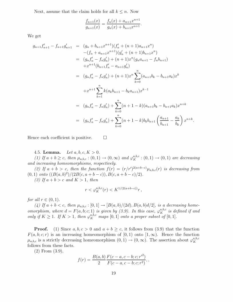
4.5. Lemma. Let a, b, c, K > 0.(1) If a + b ≥ c, then µa,b,c : (0, 1) → (0,∞) and ϕa,b,c
K : (0, 1) → (0, 1) are decreasingand increasing homeomorphisms, respectively.
(2) If a + b > c, then the function f(r) = (r/r′)2(a+b−c)µa,b,c(r) is decreasing from(0, 1) onto ((B(a, b)2)/(2B(c, a + b − c)), B(c, a + b − c)/2).
(3) If a + b > c and K > 1, then
r < ϕa,b,cK (r) < K1/(2(a+b−c))r ,
for all r ∈ (0, 1).(4) If a + b < c, then µa,b,c : [0, 1] → [B(a, b)/(2d), B(a, b)d/2], is a decreasing home-
omorphism, where d = F (a, b; c; 1) is given by (3.9). In this case, ϕa,b,cK is defined if and
only if K ≥ 1. If K > 1, then ϕa,b,cK maps [0, 1] onto a proper subset of [0, 1].
Proof. (1) Since a, b, c > 0 and a + b ≥ c, it follows from (3.9) that the functionF (a, b; c; r) is an increasing homeomorphism of [0, 1) onto [1,∞). Hence the functionµa,b,c is a strictly decreasing homeomorphism (0, 1) → (0,∞). The assertion about ϕa,b,c
K
follows from these facts.(2) From (3.9),
f(r) =B(a, b)
2
F (c − a, c − b; c; r′2)
F (c − a, c − b; c; r2), ,
19

which is decreasing with required limiting values at 0 and 1.(3) With s = ϕa,b,c
K (r) > r, from (2) we get
f(s) = (s/s′)2(a+b−c)µa,b,c(s) = (s/s′)2(a+b−c)µa,b,c(r)/K
< f(r) = (r/r′)2(a+b−c)µa,b,c(r) ,
so that(s/s′)2(a+b−c) < K(r/r′)2(a+b−c) ,
which gives s/s′ < K1/(2(a+b−c))r/r′. Hence
r < s < K1/(2(a+b−c))r(s′/r′) < K1/(2(a+b−c))r .
(4) For a, b, c > 0 and a + b < c, (3.9) implies that F (a, b; c; r) is an increasinghomeomorphism [0, 1] → [1, F (a, b; c; 1)]. Now the claim follows from (1.3) and (1.5).�
0.5 1
0.5
1 (7)
0.5 1
0.5
1 (8)
0.5 1
0.5
1 (9)
4 8
0.5
1 (4)
3 6 9
0.5
1 (5)
4 80.3
0.6
0.9 (6)
0.5 1
4
8 (1)
0.5 1
10
20 (2)
0.5 1
10
20 (3)
Figure 4: (1) µ0.5,0.5,1, (2) µ0.1,1.1,1, (3) µ2.5,1.5,2, (4) µ−10.5,0.5,1, (5) µ−1
0.1,1.1,1,
(6) µ−12.5,1.5,2, (7) ϕ0.5,0.5,1
1.5 , (8) ϕ0.1,1.1,12.5 , (9) ϕ2.5,1.5,2
3.5 .
The function µa,b,c is a natural generalization for the function µa in [AQVV, (1.3)].Namely,
µa,1−a,1(r) =B(a, 1 − a)
2
F (a, 1 − a; 1; r′2)
F (a, 1 − a; 1; r2)= µa(r) ,(4.6)
20

since by (3.4) and (3.5),
B(a, 1 − a) =Γ(a)Γ(1 − a)
Γ(1)=
π
sin(πa).
Clearly (1.3) and (1.5) imply the identities (cf. [AQVV, (4.8), (4.9)]),
µa,b,c(r)µa,b,c(r′) =
(
B(a, b)
2
)2
, r ∈ (0, 1) ,(4.7)
µ−1a,b,c(x)2 + µ−1
a,b,c(y)2 = 1 ,(4.8)
where x, y > 0 with xy = (B(a, b)/2)2, and
ϕa,b,cK (r)2 + ϕa,b,c
1/K (r′)2 = 1 .(4.9)
Moreover, from (1.3) and (3.9) we get, for c < a + b,
r′2(c−a−b)
µa,b,c(r) = r2(c−a−b)µc−a,c−b,c(r) , r ∈ (0, 1) .(4.10)
4.11. Lemma. Let f be a bijection from a real interval I onto (0,∞) and let g bedefined on I by g(x) = af(x), where a > 0 is a constant. Then for each constant K > 0,we have
f−1(Kf(x)) = g−1(Kg(x)) .
Proof. Let u = f−1(Kf(x)). Then f(u) = Kf(x), so that af(u) = aKf(x), thatis, g(u) = Kg(x). Hence u = g−1(Kg(x)). �
4.12. Remark. For a, b, c > 0 with a + b ≥ c, K > 0, and r ∈ (0, 1) denote
µa,b,c(r) =F (a, b; c; r′2)
F (a, b; c; r2)
andϕa,b,c
K (r) = µ−1a,b,c(µa,b,c(r)/K) .
By Lemma 4.11 we see thatϕa,b,c
K (r) = ϕa,b,cK (r) .
4.13. Remark. Observe first that limc→a+ B(a, c−a) = ∞ and Γ(c−a)(c−a, n) =Γ(c − a + n), which tends to Γ(n) = (n − 1)!, as c → a+.
(1) limc→a+ (Ka,c(r) − (B(a, c − a)/2)) = log(1/r′).
(2) limc→a+ (Ea,c(r) − (B(a, c − a)/2)) = log(1/r′) −(
12
∑
∞
n=1r2n
a+n−1
)
.
In particular, for each fixed r ∈ (0, 1) all the three functions Ka,c(r), Ea,c(r), andEa,c(r) − r′2Ka,c(r) tend to ∞ as c → a+.
21

4.14. Theorem. The following differentiation formulae hold:
dKa,b,c
dr=
2
rr′2(
(c − a)Ea,b,c + (br2 + a − c)Ka,b,c
)
,(4.15)
dEa,b,c
dr=
2(a − 1)
r(Ka,b,c − Ea,b,c) ,(4.16)
d
dr(Ka,b,c − Ea,b,c) =
2
rr′2
(
((c − a) − (1 − a)r′2)Ea,b,c(4.17)
+((a + b)r2 − c + r′2)Ka,b,c
)
,
d
dr(Ea,b,c − r′
2Ka,b,c) =
2
r((1 − c)Ea,b,c + (c − 1 − (b − 1)r2)Ka,b,c) ,(4.18)
d
drµa,b,c(r) = −B(a, b)M(a, b, c, r2)
rr′2v(r2)2= −B(a, b)3M(r2)
4rr′2K2 ,(4.19)
M(a, b, c, s2)
M(a, b, c, r2)
ds
dr=
1
K
ss′2v(s2)2
rr′2v(r2)2=
1
K
ss′2K(s)2
rr′2K(r)2, s = ϕa,b,c
K (r) .(4.20)
Proof. From (3.6)
dF
dz=
(c − a)u + (a − c + bz)v
z(1 − z).
Put z = r2 and multiply both sides by B(a, b)/2 . This gives (4.15).For (4.16) recall that by (3.7)
du
dz=
(a − 1)
z(v − u) .
Put z = r2 and multiply both sides by B(a, b)/2 . This gives (4.16).The formulae (4.17) and (4.18) follow from (4.15) and (4.16).From (3.10), putting z = r2, we get
M(r2) = −r2r′2dµ
dr
(
2
B(a, b)
)3
K2
(
1
2r
)
,
so thatdµ
dr= −B(a, b)3M(r2)
4rr′2K2 .
Denote s = ϕa,b,cK (r). Then by (1.5)
µa,b,c(s) =1
Kµa,b,c(r)
so thatd
dsµa,b,c(s)
ds
dr=
1
K
d
drµa,b,c(r) .
Now (4.20) follows from (4.19). �
22

4.21. Lemma. (cf. [AQVV, Lemmas 5.2 and 5.4]) For 0 < a, b < min{c, 1} andc ≤ a + b , denote K = Ka,b,c and E = Ea,b,c. Then the function
(1) f1(r) = (K−E)/(r2K) is strictly increasing from (0, 1) onto (b/c, 1). In particular,
we have the sharp inequality,b
c<
K − E
r2K< 1
for all r ∈ (0, 1).(2) f2(r) = (E − r′2K)/r2 has positive Maclaurin coefficients and maps (0, 1) onto
(B(a, b)(c − b)/(2c), C), where
C =B(a, b)B(c, c + 1 − a − b)
2B(c + 1 − a, c − b).
(3) f3(r) = r′−2(c+1−a−b)E has positive Maclaurin coefficients and maps [0, 1) onto
(B(a, b)/2,∞).
(4) f4(r) = r′2(a+b−c)K has positive Maclaurin coefficients and maps [0, 1) onto
[B(a, b)/2, B(c, a + b − c)/2).(5) f5(r) = r′−2
E has positive Maclaurin coefficients and maps [0, 1) onto[B(a, b)/2,∞).
(6) f6(r) = r′2K has negative Maclaurin coefficients, except for the constant term,and maps [0, 1) onto (0, B(a, b)/2].
(7) f7(r) = K has positive Maclaurin coefficients and is log-convex from [0, 1) onto[B(a, b)/2,∞). In fact, (d/dr)(logK) also has positive Maclaurin coefficients.
(8) f8(r) = (E − r′2K)/(r2K) is strictly decreasing from (0, 1) onto (0, 1 − (b/c)).
(9) f9(r) = (K − E)/(E − r′2K) is strictly increasing from (0, 1) onto (b/(c − b),∞).(10) f10(r) = (K − B(a, b)/2)/ log(1/r′) is strictly increasing from (0, 1) onto
(abB(a, b)/c, D), where D = 1 if c = a + b and D = ∞ if c < a + b.(11) f11(r) = (B(a, b)/2−r′2K)/r2 has positive Maclaurin coefficients and maps (0, 1)
onto (B(a, b)(c − ab)/(2c), B(a, b)/2).
(12) f12(r) = (K−B(a, b)/2)/(r′2(c−a−b) −1), for a+ b > c, is strictly increasing from(0, 1) onto (abB(a, b)/(2c(a + b − c)), B(c, a + b − c)/2).
(13) f13(r) = ((1−a−(b−c)r2)E−(1−a)r′2K)/r2 has negative Maclaurin coefficients,except for the constant term, with
f13(0+) = (c + 1 − a)(c − b)B(a, b)/(2c)
and f13(1−) = (c + 1 − a − b)E(1).(14) f14(r) = (c − a)E − (b − a)r′2K has negative Maclaurin coefficients, except for
the constant term, and maps [0, 1] onto [C, D], where
C = (c − a)E(1) and D = (c − b)B(a, b)/2.
Proof. (1) From (3.6)
dF (a−)
dz=
(a − 1)
z
(
F − F (a−))
=(a − 1)b
cF (a, b + 1; c + 1; z) .
23

Putting z = r2 and multiplying by B(a, b)/2, we get
K − E
r2=
bB(a, b)
2cF (a, b + 1; c + 1; r2) .
Hence
f1(r) =b
c
F (a, b + 1; c + 1; r2)
F (a, b; c; r2).
Thus f1(0) = b/c. The ratio of the coefficients of the numerator and denominator equals
b
c
(a, n)(b + 1, n)(c, n)
(c + 1, n)(a, n)(b, n)=
b
c
b + n
b
c
c + n=
b + n
c + n= 1 − c − b
c + n,
which is increasing in n. Hence the result follows from Theorem 4.3. The limit f1(1−) = 1follows from (3.9).
(2) From (3.6) and (3.7), we get
dF (a−)
dz=
(a − 1)
z(F − F (a−)) = (a − 1)(F +
(b − c)
cF (c+)) .
Hence putting z = r2, we get
K − E
r2= K +
(b − c)B(a, b)
2cF (a, b; c + 1; r2) .
Thus,
f2(r) =(c − b)B(a, b)
2cF (a, b; c + 1; r2) ,
which proves the assertion. The limiting values follow from (3.9).(3) By (3.9),
f3(r) =B(a, b)
2
F (a − 1, b; c; r2)
r′2(c+1−a−b)
=B(a, b)
2F (c + 1 − a, c − b; c; r2),
and the result follows.(4) By (3.9),
f4(r) =B(a, b)
2r′
2(a+b−c)F (a, b; c; r2)
=B(a, b)
2F (c − a, c − b; c; r2),
and the result follows.(5) By (3.9)
f5(r) =B(a, b)
2r′2F (a − 1, b; c; r2) =
B(a, b)
2(1 − r2)−(a+b−c)F (c + 1 − a, c − b; c; r2) ,
which is a product of two Maclaurin series with positive coefficients, hence the result.
24

(6) We have thatf6(r) = E(r) − (E(r) − r′
2K(r)) .
Hence, by (2), f6(r) − B(a, b)/2 has all Maclaurin coefficients negative.(7) The positivity of Maclaurin coefficients and the limiting values are clear. Next,
by (4.15), after simplification, we get
d
drlog K =
2r
r′2K
(
(a + b − c)K +(c − a)(E − r′2K)
r2
)
,
which has positive Maclaurin coefficients by (2) and (6).(8) f8(r) = 1 − f1(r), so that the result follows from (1).(9) f9(r) = f1(r)/f8(r), hence the result follows from (1) and (8).(10) The ratio of the coefficients equals
B(a, b)(a, n)(b, n)
(c, n)(n − 1)!≡ Tn ,
say. ThenTn+1
Tn
=(a + n)(b + n)
(c + n)n> 1 ,
so that the monotonicity follows from 4.3. The limiting values follow from (3.9).(11)
f11(r) = K − K − B/2
r2
=B
2
(
1 − ab
c+
∞∑
n=1
(
(a, n)(b, n)
(c, n)n!(1 − (a + n)(b + n)
(c + n)(n + 1))r2n
)
)
,
which has all coefficients positive. The limiting values are obvious.(12) The ratio has the indeterminate form 0/0 at r = 0. The derivative ratio equals
abB(a, b)
2c(a + b − c)
F (a + 1, b + 1; c + 1; r2)
r′2(c−a−b−1)=
abB(a, b)
2c(a + b − c)F (c − a, c − b; c + 1; r2),
by (3.9), and so the result follows by Lemma 4.1.(13) From (3.6) and (3.7)
dF (a−)
dz=
1
1 − z
(
(a − 1 + b − c)F (a−) +(c + 1 − a)(c − b)
cF (a−, c+)
)
=(a − 1)
z(F − F (a−)) .
Multiplying by z(1 − z)B(a, b)/2, we get
z(a − 1 + b − c)E +(c + 1 − a)(c − b)
czF (a−, c+)
B(a, b)
2= (a − 1)(1 − z)(K − E) .
With z = r2 this yields the result.(14) In the Gauss contiguous relation in [R1, Exercise 21(9), p. 71], if we change z to
r2 and multiply by B(a, b)/2, then we get f14(r) = ((c − b)B(a, b)/2)F (a, b − 1; c; r2), sothat the assertions on the coefficients follow. The limiting values are clear. �
25
4.22. Remark. In the classical case, a = b = 1/2 and c = 1, the boundary valuesin the above result 4.21 (13) reduce to f13(0+) = 3π/8 and f13(1−) = 1, showing thatthe above result is quite sharp.
4.23. Theorem. Let 0 < a < c ≤ 1, b = c − a, R = R(a, c − a) = −Ψ(a) − Ψ(c −a) − 2γ, and B = B(a, c − a). Then
(1) The function f(r) = Ka,c(r) + log r′ has negative Maclaurin coefficients, exceptfor the constant term, and maps [0, 1) onto (R/2, B/2].
(2) The function g(r) = Ka,c(r) + (1/r2) log r′ has positive Maclaurin coefficientsand maps (0, 1) onto ((B − 1)/2, R/2) if a, b ∈ (0, 1), while it has negative Maclaurincoefficients and maps (0, 1) onto (R/2, (B − 1)/2) if a, b ∈ (1,∞).
(3) The function h(r) = r2Ka,c(r)/ log(1/r′) is strictly decreasing (respectively, in-
creasing) from (0, 1) onto (1, B) if a, b ∈ (0, 1) (respectively, onto (B, 1), if a, b ∈ (1,∞)).(4) The function k(r) = Ka,c(r)/ log((eR/2)/r′) is strictly decreasing from (0, 1) onto
(1, B/R).
Proof. (1) That f(0+) = B(a, c − a)/2 is clear and f(1−) = R(a, c − a)/2 followsfrom [AVV, Theorem 1.52 (2)]. Next,
2f(r) = B + B
∞∑
n=1
(
(a, n)(b, n)
(c, n)n!− 1
n
)
r2n.
Thus, we need to show that Tn = (a, n)(b, n)/((c, n)(n − 1)!) < 1. Now
Tn+1
Tn=
(a + n)(b + n)
(c + n)n=
(a + b)n + n2 + ab
(a + b)n + n2> 1,
and limn→∞ Tn = 1 by Stirling’s formula. Hence Tn < 1 for all n = 1, 2, 3, . . ..(2)
g(0+) =B
2+ lim
r→0
log r′
r2=
B
2− 1
2.
Next, g(r) = f(r) + (1/r2 − 1) log r′, so that g(1−) = f(1−) = R/2, from (1). Next,
2g(r) = BF (a, b; c; r2) − 1
r2log
1
1 − r2
=
∞∑
n=0
1
n + 1
(
B(a, n)(b, n)(n + 1)
(c, n)n!− 1
)
r2n.
Let
Tn =B(a, n)(b, n)(n + 1)
(c, n)n!.
ThenTn+1
Tn=
(a + n)(b + n)(n + 2)
(c + n)(n + 1)2.
26

Now (a+n)(b+n)(n+2)− (c+n)(n+1)2 = −(1−ab)n− (a+ b−2ab), which is negative(positive) if a, b ∈ (0, 1) (a, b ∈ (1,∞)). By Stirling’s formula, limn→∞ Tn = 1. Hence theresult follows.
(3)
h(r) =g(r)
1r2 log 1
r′
+ 1,
so that h(0+) = B and h(1−) = 1 are clear. Next,
h(r) =B∑
∞
n=0(a,n)(b,n)(c,n)n!
r2n
∑
∞
n=01
n+1r2n
,
so that the coefficient ratio equals (a, n)(b, n)(n + 1)/((c, n)n!), which is decreasing ifa, b ∈ (0, 1) and increasing if a, b ∈ (1,∞). Hence the result follows from [PV, Lemma2.1].
(4) We have k(r) = 1 + (f(r)−R/2)/ log(eR/2/r′). Hence the result follows from (1).�
4.24. Theorem. (1) Let 0 < a, b < c and 2ab < c ≤ a + b < c + 1/2. Then thefunction f(r) = r′K(r) is strictly decreasing from [0, 1) onto (0, B(a, b)/2].
(2) Let 0 < a, b < c < a + b. Then the function g(r) = r′2(a+b−c)(K − E)/r2 haspositive Maclaurin coefficients and maps (0, 1) onto (bB(a, b)/(2c), B(c, a + b − c)/2).
(3) Let 0 < a, b < 1, c = a + b, and a(2b + 1) < b + 1 < 1/a. Then the functionh(r) = (K − E)/ log(1/r′) is decreasing from (0, 1) onto (1, bB(a, b)/c).
Proof. (1) Clearly f(0) = B(a, b)/2 and by (3.9), f(1) = 0. We have f(r) =g(r)/h(r), where
g(r) = B(a, b)∞∑
0
(a, n)(b, n)
(c, n)n!r2n ,
and
h(r) = 2∞∑
0
dnr2n ,
with d0 = 1 and dn = (1 · 3 · . . . · (2n− 1))/(2 · 4 · . . . · (2n)) for n = 1, 2, 3, . . .. Hence, thecoefficient ratio equals
Tn =B(a, b)(a, n)(b, n)2n
(c, n) · 1 · 3 · . . . · (2n − 1).
ThenTn+1
Tn
=2(n + 1)(n + b)
(2n + 1)(n + c).
Now
(2n + 1)(n + c) − 2(n + a)(n + b) = n(2c + 1 − 2a − 2b) + c − 2ab > 0 ,
so that Tn is decreasing and hence by Theorem 4.3, f is also decreasing.
27

(2) From (3.6), (3.9) and (4.16), we get
f(r) =bB(a, b)
2cr′
2(a+b−c)F (a, b + 1; c + 1; r2) =
bB(a, b)
2cF (c + 1 − a, c − b; c + 1; r2).
Hence the assertion follows from (3.9).(3) As in (2), from (3.6), (3.9) and (4.16), we get
h(r) =bB(a, b)
c
r2F (a, b + 1; c + 1; r2)
2 log(1/r′).
Writing the Maclaurin series expansion of both the numerator and the denominator, theratio of coefficients equals
Tn =bB(a, b)
c
(a, n)(b + 1, n)(n + 1)
(c + 1, n)n!=
B(a, b)(a, n)(b, n + 1)(n + 1)
(c, n + 1)n!.
HenceTn+1
Tn=
(a + n)(b + n + 1)(n + 2)
(c + n + 1)(n + 1)2.
Then,
(c + n + 1)(n + 1)2 − (a + n)(b + n + 1)(n + 2) = n(1 − a − ab) + (1 + b − 2ab − a) > 0.
Hence, Tn is decreasing, so that the result follows by (3.9) and Theorem 4.3. �
4.25. Remark. Theorem 4.24(3) generalizes [AQVV, Lemma 5.2 (12)]. The latterfollows if we put c = 1 in Theorem 4.24(3).
4.26. Differential equations. The hypergeometric function w = F (a, b; c; z) sat-isfies the differential equation [R1, p. 54]
z(1 − z)w′′ + (c − (a + b + 1)z)w′ − abw = 0 .
Changing the variable z to z2, this reduces to
z(1 − z2)w′′ + (2c − 1 − (2a + 2b + 1)z2)w′ − 4abzw = 0 .
In particular, the generalized elliptic integrals, w = Ka,c(r) and w = K′
a,c(r), satisfy,respectively, the differential equations
rr′2w′′ + (2c − 1 − (2c + 1)r2)w′ − 4a(c − a)rw = 0 ,(4.27)
andrr′
2w′′ − (1 − (2c + 1)r2)w′ − 4a(c − a)rw = 0 .(4.28)
In the special case c = 1 the above two equations coincide (cf. [AQVV, (4.3)], [L, 3.8.19,p. 75]). Next, the generalized elliptic integrals w = Ea,c(r) and w = E
′
a,c(r) satisfy,respectively, the differential equations
rr′2w′′ − (2c − 1)r′
2w′ + 4(1 − a)(c − a)rw = 0 ,(4.29)
28

andrr′
2w′′ − (1 + (2c − 1)r2)w′ + 4(1 − a)(c − a)rw = 0 .(4.30)
In the special case c = 1 the equations (4.29) and (4.30) are still different unlike in thecase of (4.27) and (4.28) (cf. [L, 3.8.17, p. 74 and 3.8.23, p. 75]).
4.31. Correction. In [AQVV, (4.3), p. 14] the first differential equation has asymmetry property, namely, it is satisfied both by Ka and K
′
a. However, the seconddifferential equation is satisfied only by Ea, and not by E
′
a. The differential equationsatisfied by w = E
′
a is obtained by putting c = 1 in (4.30). Thus it is
rr′2w′′ − (1 + r2)w′ + 4(1 − a)2rw = 0 .
We use the notation
Sw =
(
w′′
w′
)′
− 1
2
(
w′′
w′
)2
for the Schwarzian derivative.
4.32. Lemma. [R2, p. 9] Let w1, w2 be linearly independent solutions of the differ-ential equation w′′ + p(z)w′ + q(z)w = 0. Then W = w1/w2 satisfies the differentialequation
SW (z) = 2q(z) − p′(z) − p(z)2/2 .
4.33. Theorem. Let 0 < a, b < 1 and 2c = a + b + 1. Then the modulus µ = µa,b,c
satisfies the differential equation
Sµ(r) = 2q(r) − p′(r) − p(r)2/2 ,
where
p(r) =2c − 1 − (4c − 1)r2
rr′2, q(r) = −4ab
r′2.
Proof. Follows immediately from Lemma 4.32 and (4.27). �
4.34. Theorem. Let 0 < a, b < 1 and 2c = a + b. Then the function ν = E′/E
satisfies the differential equation
Sν(r) = 2q(r) − p′(r) − p(r)2/2 ,
where
p(r) =2c − 1 − (4c − 1)r2
rr′2, q(r) = −4(a − 1)b
r′2.
29

Proof. Follows immediately from Lemma 4.32 and (4.29). �
4.35. Lemma. If 0 < a < min{c, 1} and c ≤ a + (1/2), then the function f(r) =rKa,c(r)/arthr is strictly decreasing from (0, 1) onto (1, B/2), where B = B(a, c − a).
Proof. Let f(r) = g(r)/h(r), where g(r) = rKa,c(r) and h(r) = arth r. Theng(0) = h(0) = 0 and
g′(r)/h′(r) = 2(c − a)Ea,c(r) + (1 − 2(c − a))(r′2)Ka,c(r) ,
which, by Lemma 4.21 (6), being a sum of two strictly decreasing functions, is also so.Hence, the monotonicity follows from L’Hopital’s Monotone Rule, Lemma 4.1. Finally,f(0+) = B/2 by L’Hopital’s Rule and f(1−) = g′(1−)/h′(1−) = 1, again by L’Hopital’sRule. �
Acknowledgments. The authors wish to thank the Finnish National Academy ofScience and Letters, the Finnish Mathematical Society, and the Departments of Math-ematics at the University of Helsinki and the University of Turku for generous sup-port. The authors are indebted to Heikki Ruskeepaa for providing expert help with
the Mathematicar software. They are also grateful to D. Askey, B. C. Carlson, N.Stylianopoulos, and T. Sugawa for interesting discussions and correspondence.
References
[AS] M. Abramowitz and I. A. Stegun, editors: Handbook of Mathematical Functions
with Formulas, Graphs and Mathematical Tables, Dover, New York, 1965.
[Ah] L. V. Ahlfors: Complex Analysis, 2nd ed., McGraw-Hill, New York, 1966.
[AQVV] G. D. Anderson, S. -L. Qiu, M. K. Vamanamurthy, and M. Vuorinen: Gen-
eralized elliptic integrals and modular equations, Pacific J. Math. 192 (2000), 1–37.
[AVV] G. D. Anderson, M. K. Vamanamurthy, and M. Vuorinen: Conformal Invari-
ants, Inequalities, and Quasiconformal Maps, J. Wiley, 1997.
[AAR] G. E. Andrews, R. Askey, and R. Roy: Special Functions, Cambridge Univ.Press, 1999.
[B1] A. Baricz: Landen-type inequality for Bessel function, Comput. Methods Funct.
Theory 5 (2005), no. 2, 373–379.
[B2] A. Baricz: Functional inequalities involving special functions, J. Math. Anal. Appl.
319 (2006), 450–459.
[B3] A. Baricz: Functional inequalities involving special functions II, J. Math. Anal.
Appl. 327 (2007), 1202–1213.
30

[B4] A. Baricz: Turan type inequalities for generalized complete elliptic integrals, Math.
Z. 256 (2007), 895–911.
[Be] B. C. Berndt: Modular equations in Ramanujan’s lost notebook, Number theory,55–74, Trends Math., Birkhauser, Basel, 2000.
[BBG] B. C. Berndt, S. Bhargava and F. G. Garvan: Ramanujan’s theories of elliptic
functions to alternative bases, Trans. Amer. Math. Soc., 347 (1995), 4163–4244.
[BK] M. Biernacki and J. Krzyz: On the monotonicity of certain functionals in the
theory of analytic functions, Ann. Univ. M. Curie-Sklodowska, 2 (1955), 134–145.
[BB] J. M. Borwein and P. B. Borwein: Pi and the AGM, John Wiley & Sons, NewYork, 1987.
[Bo] F. Bowman: Introduction to Elliptic Functions with applications, English UniversitiesPress Ltd., London, 1953.
[BF] P. F. Byrd and M. D. Friedman: Handbook of Elliptic Integrals for Engineers and
Scientists, 2nd ed., Grundlehren Math. Wiss. Vol. 67, Springer-Verlag, Berlin, 1971.
[CLT] H. H. Chan, W-C. Liaw and V. Tan: Ramanujan’s class invariant λn and a new
class of series for 1/π, J. London Math. Soc. (2) 64 (2001), no. 1, 93–106.
[DV] V. N. Dubinin and M. Vuorinen: On conformal moduli of polygonal quadrilaterals,arXiv:math.CV/0701387
[HLVV] V. Heikkala, H. Linden, M. K. Vamanamurthy, and M. Vuorinen: General-ized elliptic integrals II, arXiv:math.CA/0701438
[Hen] P. Henrici: Applied and Computational Complex Analysis, Vol. III, Wiley, New York,1986.
[Her] J. Hersch: On harmonic measures, conformal moduli and some elementary symmetry
methods, J. Analyse Math. 42 (1982/83), 211–228.
[KS] D. Karp and S. M. Sitnik: Inequalities and monotonicity of ratios for generalizedhypergeometric function, arXiv:math.CA/0703084.
[L] D. F. Lawden: Elliptic Functions and Applications, Applied Math. Sciences, Vol. 80,Springer-Verlag, New York, 1989.
[LV] O. Lehto and K. I. Virtanen: Quasiconformal Mappings in the Plane, 2nd ed.,Grundlehren Math. Wiss., Band 126, Springer-Verlag, New York, 1973.
[M] A. I. Markushevich: Theory of Functions of a Complex Variable, Vol. II, Prentice-Hall, Englewood Cliffs, NJ, 1965.
[N] Z. Nehari: Conformal mapping, McGraw-Hill Book Co., Inc., New York, Toronto,London, 1952. viii+396 pp.
[PV] S. Ponnusamy and M. Vuorinen: Asymptotic expansions and inequalities for hy-
pergeometric functions, Mathematika 44 (1997), 278–301.
[Q] S. L. Qiu: Grotzsch ring and Ramanujan’s modular equations, (Chinese) Acta Math.Sinica 43 (2000), no. 2, 283–290.
31

[QV1] S. L. Qiu and M. Vuorinen: Duplication inequalities for the ratios of hypergeometric
functions, Forum Math. 12 (2000), no. 1, 109–133.
[QV2] S.-L. Qiu and M. Vuorinen: Landen inequalities for hypergeometric functions,
Nagoya Math. J. 154 (1999), 31-56.
[R1] E. D. Rainville: Special Functions, Macmillan, New York, 1960.
[R2] E. D. Rainville: Intermediate differential equations, 2nd ed. Macmillan, New York,1964.
[RV] A. Rasila and M. Vuorinen: Experiments with the moduli of quadrilaterals,arXiv:math.NA/0703149, Rev. Roumaine Math. Pures Appl. 51 (2006), 747–757,
[S] L-C. Shen: On an identity of Ramanujan based on the hypergeometric series
2F1(1/3, 2/3; 1/2;x), J. Number Theory 69 (1998), no. 2, 125–134.
[WZQC] G. Wang, X. Zhang, S.-L. Qiu, and Y. Chu: The bounds of the solutions togeneralized modular equations, J. Math. Anal. Appl. 321 (2006), 589–594.
[WW] E. T. Whittaker and G. N. Watson: A Course of Modern Analysis, 4th ed.,Cambridge Univ. Press, London, 1927.
[ZWC] X. Zhang, G. Wang, and Y. Chu: Some inequalities for the generalized Grotzschfunction, Proc. Edinburgh Math. Soc. ( to appear )
V. Heikkala
SSH Communications Security Corp.
Valimotie 17
FIN–00380 Helsinki
Finland
email: [email protected]
fax: +358-20-5007051
M.K. Vamanamurthy
Department of Mathematics
The University of Auckland
P B 92019, Auckland
New Zealand
email: [email protected]
fax: +64-9-3737457
M. Vuorinen
Department of Mathematics
FIN-20014 University of Turku
FINLAND
email: [email protected]
fax: +358-2-3336595
32