PART IV BUSINESS CYCLE THEORY: THE ECONOMY … · Learning Objectives This chapter introduces you to understanding: business cycle time horizons in Macroeconomics aggregate demand

PART IVPART IV

BUSINESS CYCLE THEORY: THE ECONOMY IN THE SHORT RUN

Chapter 9: Introduction to Economic Fluctuations 1/44

Chapter 9: Introduction to Economic Fluctuations*

MACROECONOMICS

Seventh Edition

N. Gregory Mankiw

Chapter 9: Introduction to Economic Fluctuations 2/44* Slides based on Ron Cronovich's slides, adjusted for course in Macroeconomics for International Masters Program at the Wang Yanan Institute for Studies in Economics at Xiamen University.

Learning Objectives

This chapter introduces you to understanding:

business cycle

time horizons in Macroeconomics

aggregate demand


aggregate supply

stabilization policy

• GDP growth averages 3–3.5 percent per year over the long run with large fluctuations in the short run.

9.1) Business Cycle

� Some Facts

the long run with large fluctuations in the short run.

• Consumption and investment fluctuate with GDP, but consumption tends to be less volatile and investment more volatile than GDP.

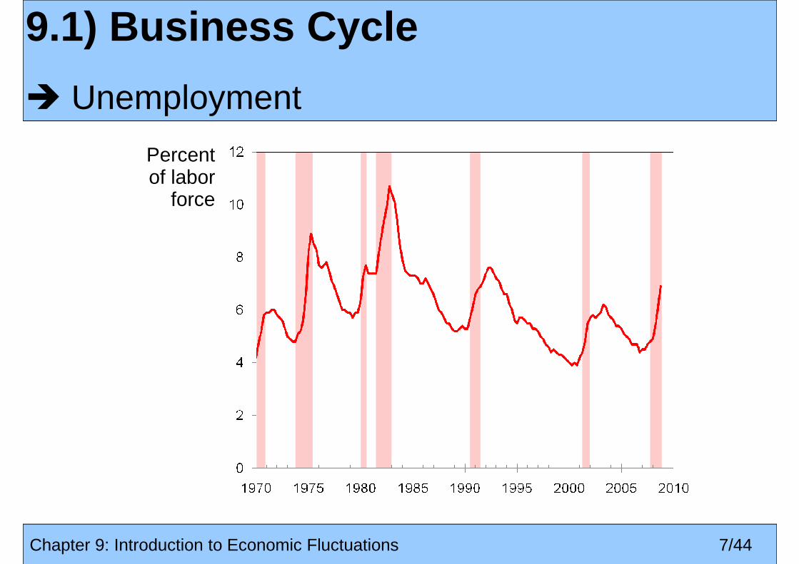
• Unemployment rises during recessions and falls during expansions.


during expansions.

• Okun’s Law : the negative relationship between GDP and unemployment.

9.1) Business Cycle

� Growth Rates of Real GDP, ConsumptionPercent change from 4

Real GDP growth rate

from 4 quarters

earlier

Average growth

rate

Consumption growth rate


9.1) Business Cycle

� Growth Rates of RGDP, C, IPercent change from 4

Investment growth rate

from 4 quarters

earlier

Real GDP growth rate

Consumption growth rate


growth rate

9.1) Business Cycle

� Unemployment

Percent of labor

force


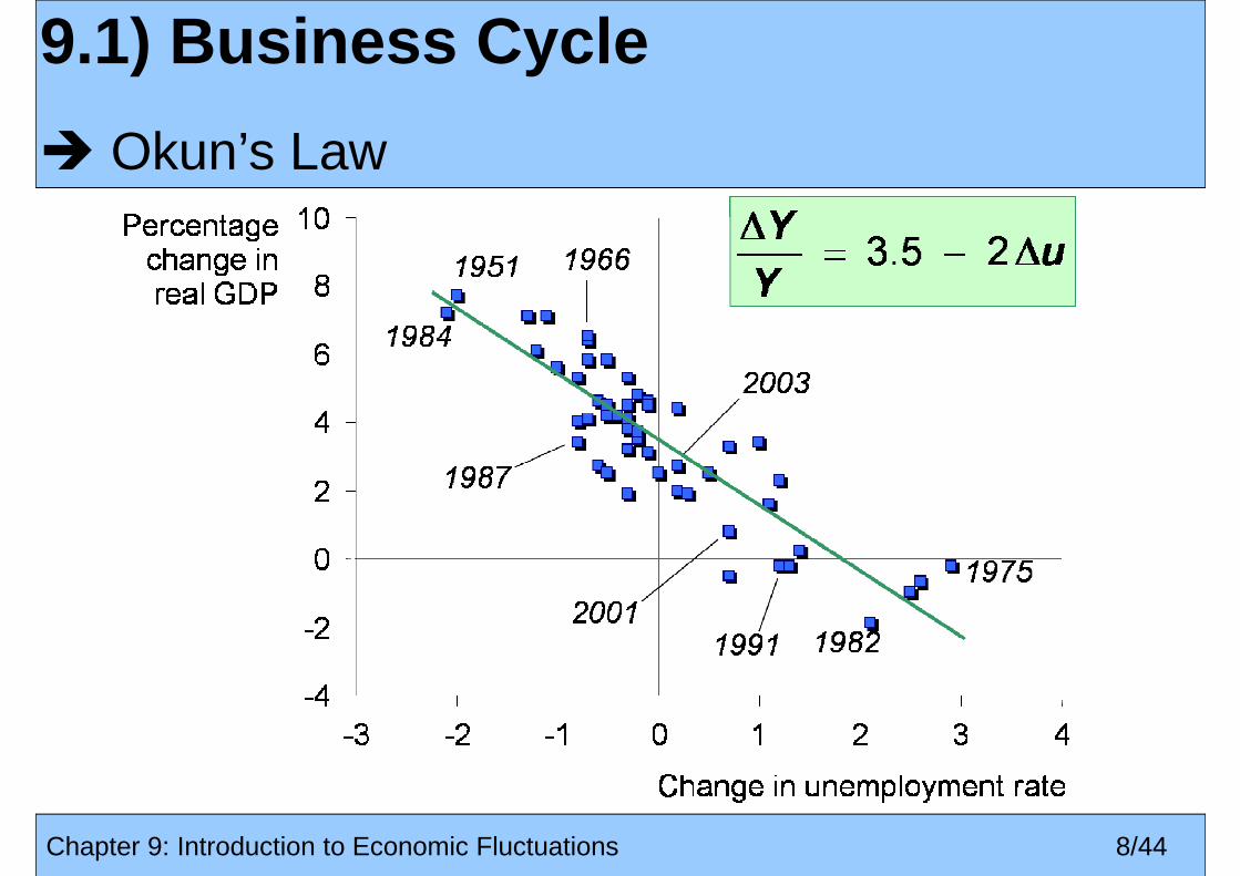
9.1) Business Cycle

� Okun’s Law


9.1) Business Cycle

� Index of Leading Economic Indicators

• Published monthly by the Conference Board.

• Aims to forecast changes in economic activity 6-9 months into the future.

• Used in planning by businesses and govt, despite not


• Used in planning by businesses and govt, despite not being a perfect predictor.

• Average workweek in manufacturing• Initial weekly claims for unemployment insurance

9.1) Business Cycle

� Components of the LEI Index

• Initial weekly claims for unemployment insurance• New orders for consumer goods and materials• New orders, nondefense capital goods• Index of supplier deliveries• New building permits issued• Index of stock prices


• Index of stock prices• M2• Yield spread (10-year minus 3-month) on Treasuries• Index of consumer expectations

9.1) Business Cycle

� Index of Leading Economic Indicators20

04 =

100


Source: Conference Board

Learning Objectives


business cycle


aggregate demand


aggregate supply


• Long run: Prices are flexible, respond to changes in supply or

9.2) Time Horizons in Macro

� Long Run and Short Run

Prices are flexible, respond to changes in supply or demand.

• Short run:Many prices are “sticky” at some predetermined level.

The economy behaves much


The economy behaves much differently when prices are sticky.

• Output is determined by the supply side:

– supplies of capital, labor


� Recap. of Classical Macro Theory (Chaps 3-8)

– supplies of capital, labor

– technology.

• Changes in demand for goods & services (C, I, G ) only affect prices, not quantities.

• Assumes complete price flexibility.

• Applies to the long run.


• Applies to the long run.


� When Prices are Sticky…

…output and employment also depend on demand, which is affected by

– fiscal policy (G and T )

– monetary policy (M )

– other factors, like exogenous changes in C or I.


– other factors, like exogenous changes in C or I.

• the paradigm most mainstream economists and


� The Model of Aggregate Demand and Supply

• the paradigm most mainstream economists and policymakers use to think about economic fluctuations and policies to stabilize the economy

• shows how the price level and aggregate output are determined


• shows how the economy’s behavior is different in the short run and long run

Learning Objectives


business cycle


aggregate demand


aggregate supply


• The aggregate demand curve shows the relationship

9.3) Aggregate Demand

� Outline

• The aggregate demand curve shows the relationship between the price level and the quantity of output demanded.

• For this chapter’s intro to the AD/AS model, we use a simple theory of aggregate demand based on the quantity theory of money.


• Chapters 10-12 develop the theory of aggregate demand in more detail.


� The Quantity Equation as Aggregate Demand

• From Chapter 4, recall the quantity equation

M V = P Y

• For given values of M and V, this equation implies an inverse relationship between P and Y .


If output increases people engage in more If output increases people engage in more


� The Downward-Sloping AD Curve

Pengage in more transactions and demand more money…

...However, at constant money supply, prices

engage in more transactions and demand more money…

...However, at constant money supply, prices


must fall to fulfill the mathematical equality from the quantity equation.

must fall to fulfill the mathematical equality from the quantity equation.

Y

AD

An increase in the An increase in the

P


� Shifting the AD Curve

An increase in the money supply shifts the ADcurve to the right.

An increase in the money supply shifts the ADcurve to the right.

AD2


Y

AD1

Learning Objectives


business cycle


aggregate demand


aggregate supply


Recall from Chapter 3:

9.4) Aggregate Supply

� Aggregate Supply in the Long Run

In the long run, output is determined by factor supplies and technology: ,= ( )Y F K L

where is the full-employment or natural level of output, the level of output at which the economy’s resources are fully employed.

Y


resources are fully employed.

“Full employment” means that unemployment equals its natural rate (not zero).

does not does not

P LRAS

Y


� The Long-Run Aggregate Supply Curve

does not depend on P, so LRAS is vertical.

does not depend on P, so LRAS is vertical.

Y


Y

( )= ,

Y

F K L

An increase in M shifts AD to

P LRAS


� Long-run Effects of an Increase in M

M shifts AD to the right.

AD

P1

P2In the long run, this raises the price level… AD2


Y

AD1

Y…but leaves output the same.

• Many prices are sticky in the short run.


� Aggregate Supply in the Short Run

• Many prices are sticky in the short run.

• For now (and through Chap. 12), we assume all prices are stuck at a predetermined level in the short run, and firms are willing to sell as much at that price level as their customers are willing to buy.


• Therefore, the short-run aggregate supply (SRAS) curve is horizontal.

The SRAS curve is horizontal:The SRAS curve is horizontal:

P


� The Short-run Aggregate Supply Curve

is horizontal:

The price level is fixed at a predetermined level, and firms sell as much as buyers demand.

is horizontal:

The price level is fixed at a predetermined level, and firms sell as much as buyers demand.

PSRAS


buyers demand.buyers demand.

Y

…an increase in aggregate

PIn the short run when prices are


� Short-run Effects of an Increase in M

aggregate demand…

AD

when prices are sticky,…

PSRAS

AD2


Y

AD1

…causes output to rise.

Y2Y1

Over time, prices gradually become “unstuck.” When they do, will they rise or fall?


� From the Short Run to the Long Run

they do, will they rise or fall?

Y Y>Y Y<

rise

fall

In the short-run equilibrium, if

then over time, P will…


Y Y= remain constant

The adjustment of prices is what moves the economy to its long-run equilibrium.

A = initial equilibrium

P LRAS


� The SR & LR Effects of ∆M > 0

AD

PSRAS

P2

A

B

CB = new short-

run eq’m after Fed increases M

AD2


Y

AD1

Y Y2

C = long-run equilibrium

• Shocks : exogenous changes in agg. supply or demand


� Shocks to Aggregate Supply and Demand

• Shocks : exogenous changes in agg. supply or demand

• Shocks temporarily push the economy away from full employment.

• Example: exogenous decrease in velocity.If the money supply is held constant, a decrease in Vmeans people will be using their money in fewer


means people will be using their money in fewer transactions, causing a decrease in demand for goods and services.

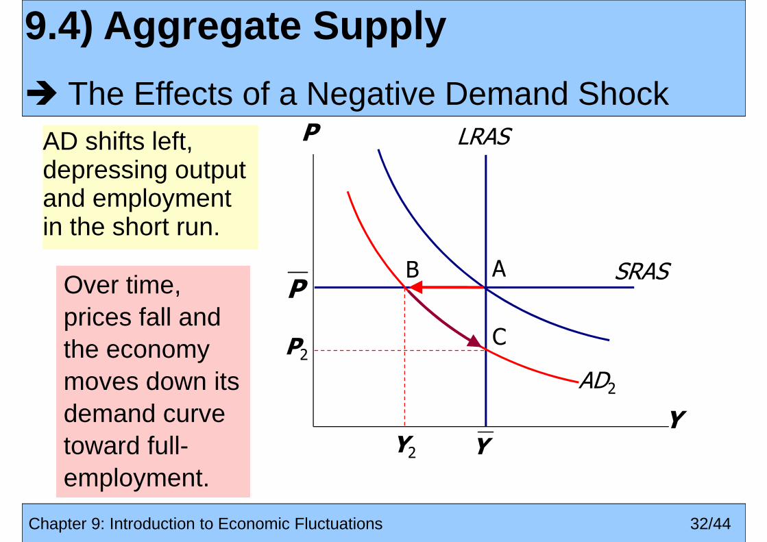
AD shifts left, depressing output AD shifts left, depressing output

LRASP


� The Effects of a Negative Demand Shock

depressing output and employment in the short run.

depressing output and employment in the short run.

PSRAS

AD1P2

AB

C

Over time, prices fall and the economy

Over time, prices fall and the economy


AD2

Y

YY2

the economy moves down its demand curve toward full-employment.

the economy moves down its demand curve toward full-employment.

• A supply shock alters production costs, affects the prices that firms charge. (also called price shocks )


� Supply Shocks

prices that firms charge. (also called price shocks )

• Examples of adverse supply shocks:

– Bad weather reduces crop yields, pushing up food prices.

– Workers unionize, negotiate wage increases.

– New environmental regulations require firms to reduce


– New environmental regulations require firms to reduce emissions. Firms charge higher prices to help cover the costs of compliance.

• Favorable supply shocks lower costs and prices.

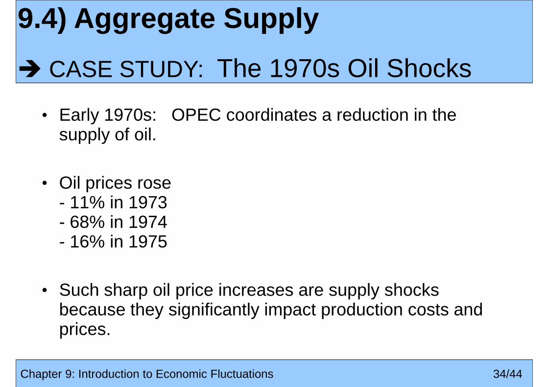
• Early 1970s: OPEC coordinates a reduction in the supply of oil.


� CASE STUDY: The 1970s Oil Shocks

supply of oil.

• Oil prices rose- 11% in 1973- 68% in 1974- 16% in 1975


• Such sharp oil price increases are supply shocks because they significantly impact production costs and prices.

The oil price shock shifts SRAS up, causing output and

The oil price shock shifts SRAS up, causing output and

P LRAS



causing output and employment to fall. causing output and employment to fall.

1P

SRAS1

AD

A

B

In absence of further price shocks, prices will fall over time and

In absence of further price shocks, prices will fall over time and

2P

SRAS2

A


Y

AD

YY2

fall over time and economy moves back toward full employment.

fall over time and economy moves back toward full employment.

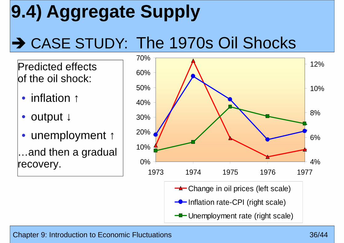
Predicted effects of the oil shock:

60%

70%12%



of the oil shock:

• inflation ↑

• output ↓

• unemployment ↑…and then a gradual recovery. 0%

10%

20%

30%

40%

50%

4%

6%

8%

10%


recovery. 0%1973 1974 1975 1976 1977

4%

Change in oil prices (left scale)

Inflation rate-CPI (right scale)

Unemployment rate (right scale)

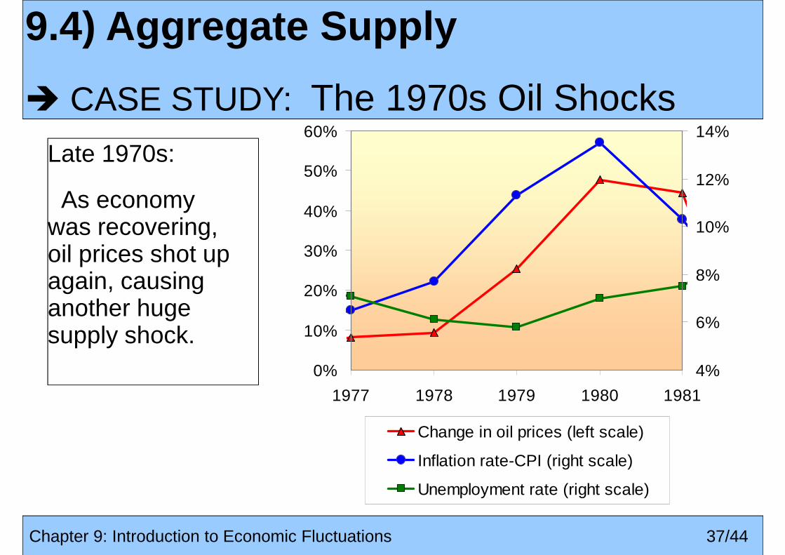
Late 1970s: 50%

60%

12%

14%



As economy was recovering, oil prices shot up again, causing another huge supply shock.

0%

10%

20%

30%

40%

4%

6%

8%

10%

12%


0%

1977 1978 1979 1980 1981

4%




1980s:

A favorable 20%

30%

40%

8%

10%



A favorable supply shock--a significant fall in oil prices.

As the model predicts, inflation and -50%

-40%

-30%

-20%

-10%

0%

10%

20%

0%

2%

4%

6%

8%


inflation and unemployment fell:

-50%

1982 1983 1984 1985 1986 1987

0%




Learning Objectives


business cycle


aggregate demand


aggregate supply


• Definition: policy actions aimed at reducing the severity

9.5) Stabilization Policy

� Definition and Example

• Definition: policy actions aimed at reducing the severity of short-run economic fluctuations.

• Example: Using monetary policy to combat the effects of adverse supply shocks:


P LRAS


� Stabilizing Output with Monetary Policy

1P

SRAS1

AD1

B

A

The adverse supply shock moves the economy to point B.

The adverse supply shock moves the economy to point B.

2P

SRAS2


Y

AD1

Y2 Y

P LRASBut the Fed accommodates But the Fed accommodates


� Stabilizing Output with Monetary Policy

1P

AD1

B

A

C

accommodates the shock by raising agg. demand.

accommodates the shock by raising agg. demand.

Results: P is permanently Results: P is permanently

2P

SRAS2

AD2


Y

AD1

Y2 Y

P is permanently higher, but Yremains at its full-employment level.

P is permanently higher, but Yremains at its full-employment level.

Chapter SummaryChapter Summary

1. Long run: prices are flexible, output and employment are always at their natural rates, and the classical theory always at their natural rates, and the classical theory applies.

Short run: prices are sticky, shocks can push output and employment away from their natural rates.

2. Aggregate demand and supply: a framework to analyze economic fluctuations


a framework to analyze economic fluctuations

3. The aggregate demand curve slopes downward.

Chapter SummaryChapter Summary

4. The long-run aggregate supply curve is vertical, because 4. The long-run aggregate supply curve is vertical, because output depends on technology and factor supplies, but not prices.

5. The short-run aggregate supply curve is horizontal, because prices are sticky at predetermined levels.

6. Shocks to aggregate demand and supply cause


6. Shocks to aggregate demand and supply cause fluctuations in GDP and employment in the short run.

7. The Fed can attempt to stabilize the economy with monetary policy.

Documents

PART IV BUSINESS CYCLE THEORY: THE ECONOMY … · Learning Objectives This chapter introduces you to understanding: business cycle time horizons in Macroeconomics aggregate demand