Part III - Combinatorics1 Hall’s theorem III Combinatorics 1 Hall’s theorem We shall begin with a discussion of Hall’s theorem. Ideally, you’ve already met it in IID Graph

Part III — Combinatorics

Based on lectures by B. BollobasNotes taken by Dexter Chua

Michaelmas 2017

These notes are not endorsed by the lecturers, and I have modified them (oftensignificantly) after lectures. They are nowhere near accurate representations of what

was actually lectured, and in particular, all errors are almost surely mine.

What can one say about a collection of subsets of a finite set satisfying certain conditionsin terms of containment, intersection and union? In the past fifty years or so, a goodmany fundamental results have been proved about such questions: in the course weshall present a selection of these results and their applications, with emphasis on theuse of algebraic and probabilistic arguments.

The topics to be covered are likely to include the following:

– The de Bruijn–Erdos theorem and its extensions.

– The Graham–Pollak theorem and its extensions.

– The theorems of Sperner, EKR, LYMB, Katona, Frankl and Furedi.

– Isoperimetric inequalities: Kruskal–Katona, Harper, Bernstein, BTBT, and theirapplications.

– Correlation inequalities, including those of Harris, van den Berg and Kesten, andthe Four Functions Inequality.

– Alon’s Combinatorial Nullstellensatz and its applications.

– LLLL and its applications.

Pre-requisites

The main requirement is mathematical maturity, but familiarity with the basic graph

theory course in Part II would be helpful.

1

Contents III Combinatorics

Contents

1 Hall’s theorem 3

2 Sperner systems 6

3 The Kruskal–Katona theorem 11

4 Isoperimetric inequalities 16

5 Sum sets 22

6 Projections 24

7 Alon’s combinatorial Nullstellensatz 29

Index 35

2

1 Hall’s theorem III Combinatorics

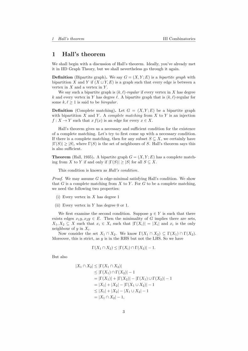
1 Hall’s theorem

We shall begin with a discussion of Hall’s theorem. Ideally, you’ve already metit in IID Graph Theory, but we shall nevertheless go through it again.

Definition (Bipartite graph). We say G = (X,Y ;E) is a bipartite graph withbipartition X and Y if (X t Y,E) is a graph such that every edge is between avertex in X and a vertex in Y .

We say such a bipartite graph is (k, `)-regular if every vertex in X has degreek and every vertex in Y has degree `. A bipartite graph that is (k, `)-regular forsome k, ` ≥ 1 is said to be biregular .

Definition (Complete matching). Let G = (X,Y ;E) be a bipartite graphwith bipartition X and Y . A complete matching from X to Y is an injectionf : X → Y such that x f(x) is an edge for every x ∈ X.

Hall’s theorem gives us a necessary and sufficient condition for the existenceof a complete matching. Let’s try to first come up with a necessary condition.If there is a complete matching, then for any subset S ⊆ X, we certainly have|Γ(S)| ≥ |S|, where Γ(S) is the set of neighbours of S. Hall’s theorem says thisis also sufficient.

Theorem (Hall, 1935). A bipartite graph G = (X,Y ;E) has a complete match-ing from X to Y if and only if |Γ(S)| ≥ |S| for all S ⊆ X.

This condition is known as Hall’s condition.

Proof. We may assume G is edge-minimal satisfying Hall’s condition. We showthat G is a complete matching from X to Y . For G to be a complete matching,we need the following two properties:

(i) Every vertex in X has degree 1

(ii) Every vertex in Y has degree 0 or 1.

We first examine the second condition. Suppose y ∈ Y is such that thereexists edges x1y, x2y ∈ E. Then the minimality of G implies there are sets,X1, X2 ⊆ X such that xi ∈ Xi such that |Γ(Xi)| = |Xi| and xi is the onlyneighbour of y in Xi.

Now consider the set X1 ∩ X2. We know Γ(X1 ∩ X2) ⊆ Γ(X1) ∩ Γ(X2).Moreover, this is strict, as y is in the RHS but not the LHS. So we have

Γ(X1 ∩X2) ≤ |Γ(Xi) ∩ Γ(X2)| − 1.

But also

|X1 ∩X2| ≤ |Γ(X1 ∩X2)|≤ |Γ(X1) ∩ Γ(X2)| − 1

= |Γ(X1)|+ |Γ(X2)| − |Γ(X1) ∪ Γ(X2)| − 1

= |X1|+ |X2| − |Γ(X1 ∪X2)| − 1

≤ |X1|+ |X2| − |X1 ∪X2| − 1

= |X1 ∩X2| − 1,

3


which contradicts Hall’s condition.One then sees that the first condition is also satisfied — if x ∈ X is a vertex,

then the degree of x certainly cannot be 0, or else |Γ({x})| < |{x}|, and we seethat d(x) cannot be > 1 or else we can just remove an edge from x withoutviolating Hall’s condition.

We shall now describe some consequences of Hall’s theorem. They willbe rather straightforward applications, but we shall later see they have someinteresting consequences.

Let A = {A1, . . . , Am} be a set system. All sets are finite. A set of distinctrepresentatives of A is a set {a1, . . . am} of distinct elements ai ∈ Ai.

Under what condition do we have a set of distinct representatives? If wehave one, then for any I ⊆ [m] = {1, 2, . . . ,m}, we have∣∣∣∣∣⋃

i∈IAi

∣∣∣∣∣ ≥ |I|.We might hope this is sufficient.

Theorem. A has a set of distinct representatives iff for all B ⊆ A, we have∣∣∣∣∣ ⋃B∈B

B

∣∣∣∣∣ ≥ |B|.This is an immediate consequence of Hall’s theorem.

Proof. Define a bipartite graph as follows — we let X = A, and Y =⋃

i∈[m]Ai.Then draw an edge from x to Ai if x ∈ Ai. Then there is a complete matchingof this graph iff A has a set of distinct representations, and the condition in thetheorem is exactly Hall’s condition. So we are done by Hall’s theorem.

Theorem. Let G = (X,Y ;E) be a bipartite graph such that d(x) ≥ d(y) forall x ∈ X and y ∈ Y . Then there is a complete matching from X to Y .

Proof. Let d be such that d(x) ≥ d ≥ d(y) for all x ∈ X and y ∈ Y . For S ⊆ Xand T ⊆ Y , we let e(S, T ) be the number of edges between S and T . Let S ⊆ X,and T = Γ(S). Then we have

e(S, T ) =∑x∈S

d(x) ≥ d|S|,

but on the other hand, we have

e(S, T ) ≤∑y∈T

d(y) ≤ d|T |.

So we find that |T | ≥ |S|. So Hall’s condition is satisfied.

Corollary. If G = (X,Y ;E) is a (k, `)-regular bipartite graph with 1 ≤ ` ≤ k,then there is a complete matching from X to Y .

Theorem. Let G = (X,Y ;E) be biregular and A ⊆ X. Then

|Γ(A)||Y |

≥ |A||X|

.

4


Proof. Suppose G is (k, `)-regular. Then

k|A| = e(A,Γ(A)) ≤ `|Γ(A)|.

Thus we have|Γ(A)||Y |

≥ k|A|`|Y |

.

On the other hand, we can count that

|E| = |X|k = |Y |`,

and sok

`=|Y ||X|

.

So we are done.

Briefly, this says biregular graphs “expand”.

Corollary. Let G = (X,Y ;E) be biregular and let |X| ≤ |Y |. Then there is acomplete matching of X into Y .

In particular, for any biregular graph, there is always a complete matchingfrom one side of the graph to the other.

Notation. Given a set X, we write X(r) for the set of all subsets of X with relements, and similarly for X(≥r) and X(≤r).

If |X| = n, then |X(r)| =(nr

).

Now given a set X and two numbers r < s, we can construct a biregulargraph (X(r), X(s);E), where A ∈ X(r) is joined to B ∈ X(s) if A ⊆ B.

Corollary. Let 1 ≤ r < s ≤ |X| = n. Suppose |n2 − r| ≥ |n2 − s|. Then there

exists an injection f : X(r) → X(s) such that A ⊆ f(A) for all A ∈ X(r).If |n2 − r| ≤ |

n2 − s|, then there exists an injection g : X(s) → X(r) such that

A ⊇ g(A) for all A ∈ X(s).

Proof. Note that |n2 − r| ≤ |n2 − s| iff

(nr

)≥(ns

).

5

2 Sperner systems III Combinatorics

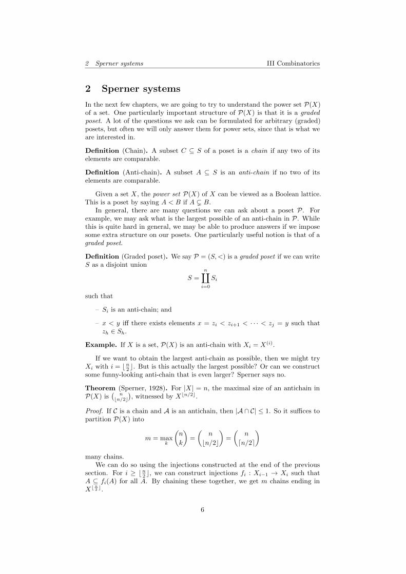
2 Sperner systems

In the next few chapters, we are going to try to understand the power set P(X)of a set. One particularly important structure of P(X) is that it is a gradedposet. A lot of the questions we ask can be formulated for arbitrary (graded)posets, but often we will only answer them for power sets, since that is what weare interested in.

Definition (Chain). A subset C ⊆ S of a poset is a chain if any two of itselements are comparable.

Definition (Anti-chain). A subset A ⊆ S is an anti-chain if no two of itselements are comparable.

Given a set X, the power set P(X) of X can be viewed as a Boolean lattice.This is a poset by saying A < B if A ( B.

In general, there are many questions we can ask about a poset P. Forexample, we may ask what is the largest possible of an anti-chain in P. Whilethis is quite hard in general, we may be able to produce answers if we imposesome extra structure on our posets. One particularly useful notion is that of agraded poset.

Definition (Graded poset). We say P = (S,<) is a graded poset if we can writeS as a disjoint union

S =

n∐i=0

Si

such that

– Si is an anti-chain; and

– x < y iff there exists elements x = zi < zi+1 < · · · < zj = y such thatzh ∈ Sh.

Example. If X is a set, P(X) is an anti-chain with Xi = X(i).

If we want to obtain the largest anti-chain as possible, then we might tryXi with i = bn2 c. But is this actually the largest possible? Or can we constructsome funny-looking anti-chain that is even larger? Sperner says no.

Theorem (Sperner, 1928). For |X| = n, the maximal size of an antichain inP(X) is

(nbn/2c

), witnessed by Xbn/2c.

Proof. If C is a chain and A is an antichain, then |A ∩ C| ≤ 1. So it suffices topartition P(X) into

m = maxk

(n

k

)=

(n

bn/2c

)=

(n

dn/2e

)many chains.

We can do so using the injections constructed at the end of the previoussection. For i ≥ bn2 c, we can construct injections fi : Xi−1 → Xi such thatA ⊆ fi(A) for all A. By chaining these together, we get m chains ending inXb

n2 c.

6


Similarly, we can partition X(≤bn/2c) into m chains with each chain endingin X(bn/2c). Then glue them together.

Another way to prove this result is to provide an alternative measure on howlarge an antichain can be, and this gives a stronger result.

Theorem (LYM inequality). Let A be an antichain in P(X) with |X| = n.Then

n∑r=0

|A ∩X(r)|(nr

) ≤ 1.

In particular, |A| ≤ maxr

(nr

)=(

nbn/2c

), as we already know.

Proof. A chain C0 ⊆ C1 ⊆ · · · ⊆ Cm is maximal if it has n + 1 elements.Moreover, there are n! maximal chains, since we start with the empty set andthen, given Ci, we produce Ci+1 by picking one unused element and adding itto Ci.

For every maximal chain C, we have |C ∩ A| ≤ 1. Moreover, every set of kelements appears in k!(n− k)! maximal chains, by a similar counting argumentas above. So ∑

A∈A|A|!(n− |A|)! ≤ n!.

Then the result follows.

There are analogous results for posets more general than just P(X). Toformulate these results, we must introduce the following new terminology.

Definition (Shadow). Given A ⊆ Si, the shadow at level i− 1 is

∂A = {x ∈ Si−1 : x < y for some y ∈ A}.

Definition (Downward-expanding poset). A graded poset P = (S,<) is said tobe downward-expanding if

|∂A||Si−1|

≥ |A||Si|

for all A ⊆ Ai.We similarly define upward-expanding , and say a poset is expanding if it is

upward or downward expanding.

Definition (Weight). The weight of a set A ⊆ S is

w(A) =

n∑i=0

|A ∩ Si||Si|

.

The theorem is that the LYM inequality holds in general for any downwardexpanding posets.

7


Theorem. If P is downward expanding and A is an anti-chain, then w(A) ≤ 1.In particular, |A| ≤ maxi |Si|.

Since each Si is an anti-chain, the largest anti-chain has size maxi |Si|.

Proof. We define the span of A to be

spanA = maxAj 6=∅

j − minAi 6=∅

i.

We do induction on spanA.If spanA = 0, then we are done. Otherwise, let hi = maxAj 6=0 j, and set

Bh−1 = ∂Ah. Then since A is an anti-chain, we know Ah−1 ∩Bh−1 = ∅.We set A′ = A\Ah∪Bh−1. This is then another anti-chain, by the transitivity

of <. We then have

w(A) = w(A′) + w(Ah)− w(Bh−1) ≤ w(A′) ≤ 1,

where the first inequality uses the downward-expanding hypothesis and thesecond is the induction hypothesis.

We may want to mimic our other proof of the fact that the largest size of anantichain in P(X) is

(nbn/2c

). This requires the notion of a regular poset.

Definition (Regular poset). We say a graded poset (S,<) is regular if for eachi, there exists ri, si such that if x ∈ Ai, then x dominates ri elements at leveli− 1, and is dominated by si elements at level i+ 1.

Proposition. An anti-chain in a regular poset has weight ≤ 1.

Proof. Let M be the number of maximal chains of length (n+ 1), and for eachx ∈ Sk, let m(x) be the number of maximal chains through x. Then

m(x) =

k∏i=1

ri

n−1∏i=k

si.

So if x, y ∈ Si, then m(x) = m(y).Now since every maximal chain passes through a unique element in Si, for

each x ∈ Si, we have

M =∑x∈Si

m(x) = |Si|m(x).

This gives the formula

m(x) =M

|Si|.

now let A be an anti-chain. Then A meets each chain in ≤ 1 elements. So wehave

M =∑

maximal chains

1 ≥∑x∈A

m(x) =

n∑i=0

|A ∩ Si| ·M

|Si|.

So it follows that ∑ |A ∩ Si||Si|

≤ 1.

8


Let’s now turn to a different problem. Suppose x1, . . . , xn ∈ C, with each|xi| ≥ 1. Given A ⊆ [n], we let

xA =∑i∈A

xi.

We now seek the largest size of A such that |xA − xB | < 1 for all A,B ∈ A.More precisely, we want to find the best choice of x1, . . . , xn and A so that |A|is as large as possible while satisfying the above condition.

If we are really lazy, then we might just choose xi = 1 for all i. By takingA = [n]bn/2c, we can obtain |A| =

(nbn/2c

).

Erdos noticed this is the best bound if we require the xi to be real.

Theorem (Erdos, 1945). Let xi be all real, |xi| ≥ 1. For A ⊆ [n], let

xA =∑i∈A

xi.

Let A ⊆ P(n). Then |A| ≤(

nbn/2c

).

Proof. We claim that we may assume xi ≥ 1 for all i. To see this, suppose weinstead had x1 = −2, say. Then whether or not i ∈ A determines whether xAshould include 0 or −2 in the sum. If we replace xi with 2, then whether or noti ∈ A determines whether xA should include 0 or 2. So replacing xi with 2 justessentially shifts all terms by 2, which doesn’t affect the difference.

But if we assume that xi ≥ 1 for all i, then we are done, since A must be ananti-chain, for if A,B ∈ A and A ( B, then xB − xA = xB\A ≥ 1.

Doing it for complex numbers is considerably harder. In 1970, Kleitmanfound a gorgeous proof for every normed space. This involves the notion of asymmetric decomposition. To motivate this, we first consider the notion of asymmetric chain.

Definition (Symmetric chain). We say a chain C = {Ci, Ci+1, . . . , Cn−i} issymmetric if |Cj | = j for all j.

Theorem. P(n) has a decomposition into symmetric chain.

Proof. We prove by induction. In the case n = 1, we simply have to take{∅, {1}}.

Now suppose P(n − 1) has a symmetric chain decomposition C1 ∪ · · · ∪ Ct.Given a symmetric chain

Cj = {Ci, Ci+1, . . . , Cn−1−i},

we obtain two chains C(0)j , C(1)j in P(n) by

C(0)j = {Ci, Ci+1, . . . , Cn−1−i, Cn−1−i ∪ {n}}

C(1)j = {Ci ∪ {n}, Ci+1 ∪ {n}, . . . , Cn−2−i ∪ {n}}.

Note that if |Cj | = 1, then C(1)j = ∅, and we drop this. Under this convention, we

note that every A ∈ P(n) appears in exactly one C(ε)j , and so we are done.

9


We are not going to actually need the notion of symmetric chains in ourproof. What we need is the “profile” of a symmetric chain decomposition. By asimple counting argument, we see that for 0 ≤ i ≤ n

2 , the number of chains withn+ 1− 2i sets is

`(n, i) ≡(n

i

)−(

n

i− 1

).

Theorem (Kleitman, 1970). Let x1, x2, . . . , xn be vectors in a normed spacewith norm ‖xI‖ ≥ 1 for all i. For A ∈ P(n), we set

xA =∑i∈A

xi.

Let A ⊆ P(n) be such that ‖xA − xB‖ < 1. Then ‖A‖ ≤(

nbn/2c

).

This bound is indeed the best, since we can pick xi = x for some ‖x‖ ≥ 1,and then we can pick A = [n]bn/2c.

Proof. Call F ⊆ P(n) sparse if ‖xE − xF ‖ ≥ 1 for all E,F ∈ F , E 6= F . Notethat if F is sparse, then |F ∩ A| ≤ 1. So if we can find a decomposition of P(n)into

(nbn/2c

)sparse sets, then we are done.

We call a partition P(n) = F1 ∪ · · · ∪ Ft symmetric if the number of familieswith n + 1 − 2i sets is `(n, i), i.e. the “profile” is that of a symmetric chaindecomposition.

Claim. P(n) has a symmetric decomposition into sparse families.

We again induct on n. When n = 1, we can take {∅, {1}}. Now suppose∆n−1 is a symmetric decomposition of P(n− 1) as F1 ∪ · · · ∪ Ft.

Given Fj , we construct F (0)j and F (1)

j “as before”. We pick some D ∈ Fj , tobe decided later, and we take

F (0)j = Fj ∪ {D ∪ {n}}

F (1)j = {E ∪ {n} : E ∈ Fj \ {D}}.

The resulting set is certainly still symmetric. The question is whether it is sparse,

and this is where the choice of D comes in. The collection F (1)j is certainly still

sparse, and we must pick a D such that F (0)j is sparse.

To do so, we use Hahn–Banach to obtain a linear functional f such that‖f‖ = 1 and f(xn) = ‖xn‖ ≥ 1. We can then pick D to maximize f(xD). Thenwe check that if E ∈ Fj , then

f(xD∪{n} − x2) = f(xD)− f(xE) + f(xn).

By assumption, f(xn) ≥ 1 and f(xD) ≥ f(xE). So this is ≥ 1. Since ‖f‖ = 1, itfollows that ‖xD∪{n} − xE‖ ≥ 1.

10

3 The Kruskal–Katona theorem III Combinatorics

3 The Kruskal–Katona theorem

For A ⊆ X(r), recall we defined the lower shadow to be

∂A = {B ∈ X(r−1) : B ⊆ A for some A ∈ A}.

The question we wish to understand is how small we can make ∂A, relative toA. Crudely, we can bound the size by

|∂A| ≥ |A|(

nr−1)(

nr

) =n− rr|A|.

But surely we can do better than this. To do so, one reasonable strategy is tofirst produce some choice of A we think is optimal, and see how we can provethat it is indeed optimal.

To do so, let’s look at some examples.

Example. Take n = 6 and r = 3. We pick

A = {123, 456, 124, 256}.

Then we have∂A = {12, 13, 23, 45, 46, 56, 14, 24, 25, 26},

and this has 10 elements.But if we instead had

A = {123, 124, 134, 234},

then∂A = {12, 13, 14, 23, 24, 34},

and this only has 6 elements, and this is much better.

Intuitively, the second choice of A is better because the terms are “bunched”together.

More generally, we would expect that if we have |A| =(kr

), then the best

choice should be A = [k](r), with |∂A| =(

kr−1). For other choices of A, perhaps

a reasonable strategy is to find the largest k such that(kr

)< |A|, and then take

A to be [k](r) plus some elements. To give a concrete description of which extraelements to pick, our strategy is to define a total order on [n](r), and say weshould pick the initial segment of length |A|.

This suggests the following proof strategy:

(i) Come up with a total order on [n](r), or even N(r) such that [k](r) areinitial segments for all k.

(ii) Construct some “compression” operators P(N(r))→ P(N(r)) that pusheseach element down the ordering without increasing the |∂A|.

(iii) Show that the only subsets of N(r) that are fixed by the compressionoperators are the initial segments.

There are two natural orders one can put on [n](r):

11


– lex: We say A < B if minA∆B ∈ A.

– colex: We say A < B if maxA∆B ∈ B.

Example. For r = 3, the elements of X(3) in colex order are

123, 124, 134, 234, 125, 135, 235, 145, 245, 345, 126, . . .

In fact, colex is an order on N(r), and we see that the initial segment with(nr

)elements is exactly [n](r). So this is a good start.If we believe that colex is indeed the right order to do, then we ought to

construct some compression operators. For i 6= j, we define the (i, j)-compressionas follows: for a set A ∈ X(r), we define

Cij(A) =

{(A \ {j}) ∪ {i} j ∈ A, i 6∈ AA otherwise

For a set system, we define

Cij(A) = {Cij(A) : A ∈ A} ∪ {A ∈ A : Cij(A) ∈ A}

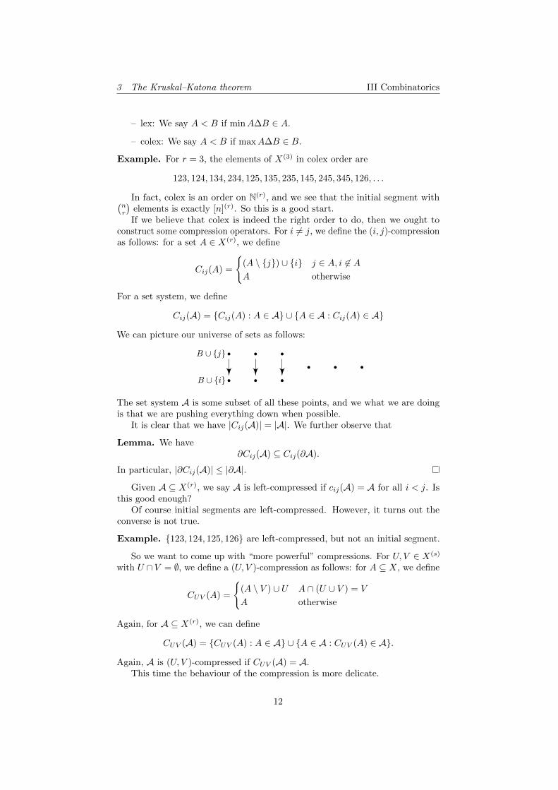
We can picture our universe of sets as follows:

B ∪ {j}

B ∪ {i}

The set system A is some subset of all these points, and we what we are doingis that we are pushing everything down when possible.

It is clear that we have |Cij(A)| = |A|. We further observe that

Lemma. We have∂Cij(A) ⊆ Cij(∂A).

In particular, |∂Cij(A)| ≤ |∂A|.

Given A ⊆ X(r), we say A is left-compressed if cij(A) = A for all i < j. Isthis good enough?

Of course initial segments are left-compressed. However, it turns out theconverse is not true.

Example. {123, 124, 125, 126} are left-compressed, but not an initial segment.

So we want to come up with “more powerful” compressions. For U, V ∈ X(s)

with U ∩V = ∅, we define a (U, V )-compression as follows: for A ⊆ X, we define

CUV (A) =

{(A \ V ) ∪ U A ∩ (U ∪ V ) = V

A otherwise

Again, for A ⊆ X(r), we can define

CUV (A) = {CUV (A) : A ∈ A} ∪ {A ∈ A : CUV (A) ∈ A}.

Again, A is (U, V )-compressed if CUV (A) = A.This time the behaviour of the compression is more delicate.

12


Lemma. Let A ⊆ X(r) and U, V ∈ X(s), U ∩ V = ∅. Suppose for all u ∈ U ,there exists v such that A is (U \ {u}, V \ {v})-compressed. Then

∂CUV (A) ⊆ CUV (∂A). �

Lemma. A ⊆ X(r) is an initial segment of X(r) in colex if and only if it is(U, V )-compressed for all U, V disjoint with |U | = |V | and maxV > maxU .

Proof. ⇒ is clear. Suppose A is (U, V ) compressed for all such U, V . If A is notan initial segment, then there exists B ∈ A and C 6∈ A such that C < B. ThenA is not (C \B,B \ C)-compressed. A contradiction.

Lemma. Given A ∈ X(r), there exists B ⊆ X(r) such that B is (U, V )-compressed for all |U | = |V |, U ∩ V = ∅, maxV > maxU , and moreover

|B| = |A|, |∂B| ≤ |∂A|. (∗)

Proof. Let B be such that ∑B∈B

∑i∈B

2i

is minimal among those B’s that satisfy (∗). We claim that this B will do. Indeed,if there exists (U, V ) such that |U | = |V |, maxV > maxU and CUV (B) 6= B,then pick such a pair with |U | minimal. Then apply a (U, V )-compression, whichis valid since given any u ∈ U we can pick any v ∈ V that is not maxV to satisfythe requirements of the previous lemma. This decreases the sum, which is acontradiction.

From these, we conclude that

Theorem (Kruskal 1963, Katona 1968). Let A ⊆ X(r), and let C ⊆ X(r) bethe initial segment with |C| = |A|. Then

|∂A| ≥ |∂C|.

We can now define the shadow function

∂(r)(m) = min{|∂A| : A ⊆ X(r), |A| = m}.

This does not depend on the size of X as long as X is large enough to accommo-date m sets, i.e.

(nr

)≥ m. It would be nice if we can concretely understand this

function. So let’s try to produce some initial segments.Essentially by definition, an initial segment is uniquely determined by the

last element. So let’s look at some examples.

Example. Take r = 4. What is the size of the initial segment ending in 3479?We note that anything that ends in something less than 8 is less that 3479,and there are

(84

)such elements. If you end in 9, then you are still fine if the

second-to-last digit is less than 7, and there are(63

)such elements. Continuing,

we find that there are (8

4

)+

(6

3

)+

(4

2

)such elements.

13


Given mr > mr−1 > · · · > ms ≥ s, we letB(r)(mr,mr−1, . . . ,ms) be theinitial segment ending in the element

mr + 1,mr−1 + 1, . . . ,ms+1 + 1,ms,ms − 1,ms − 2, . . . ,ms − (s− 1).

This consists of the sets {a1 < a2 < · · · < ar} such that there exists j ∈ [s, r]with ai = mi + 1 for i > j, and aj ≤ mj .

To construct an element in B(r)(mr, . . . ,ms), we need to first pick a j, andthen select j elements that are ≤ mj . Thus, we find that

|B(r)(mr, . . . ,ms)| =r∑

j=s

(mj

j

)= b(r)(m1, . . . ,ms).

We see that this B(r) is indeed the initial segment in the colex order endingin that element. So we know that for all m ∈ N, there is a unique sequencemr > mr−1 > . . . , > ms ≥ s such that n =

∑rj=0

(mj

j

).

It is also not difficult to find the shadow of this set. After a bit of thinking,we see that it is given by

B(r−1)(mr, . . . ,ms).

Thus, we find that

∂(r)

(r∑

i=s

(mi

i

))=

r∑i=s

(mi

i− 1

),

and moreover every m can be expressed in the form∑r

i=s

(mi

i

)for some unique

choices of mi.In particular, we have

∂(r)((

n

r

))=

(n

r − 1

).

Since it might be slightly annoying to write m in the form∑r

i=s

(mi

i

), Lovasz

provided another slightly more convenient bound.

Theorem (Lovasz, 1979). If A ⊆ X(r) with |A| =(xr

)for x ≥ 1, x ∈ R, then

|∂A| ≥(

x

r − 1

).

This is best possible if x is an integer.

Proof. Let

A0 = {A ∈ A : 1 6∈ A}A1 = {A ∈ A : 1 ∈ A}.

For convenience, we write

A1 − 1 = {A \ {1} : A ∈ A1}.

We may assume A is (i, j)-compressed for all i < j. We induct on r and then on|A|. We have

|A0| = |A| − |A1|.

14


We note that A1 is non-empty, as A is left-compressed. So |A0| < |A|.If r = 1 and |A| = 1 then there is nothing to do.Now observe that ∂A ⊆ A1 − 1, since if A ∈ A, 1 6∈ A, and B ⊆ A is such

that |A \ B| = 1, then B ∪ {1} ∈ A1 since A is left-compressed. So it followsthat

|∂A0| ≤ |A1|.

Suppose |A1| <(x−1r−1). Then

|A0| >(x

r

)−(x− 1

r − 1

)=

(x− 1

r

).

Therefore by induction, we have

|∂A0| >(x− 1

r − 1

).

This is a contradiction, since |∂A0| ≤ |A1|. Hence |A1| ≥(x−1r−1). Hence we are

done, since

|∂A| ≥ |∂A1| = |A1|+ |∂(A1 − 1)| ≥(x− 1

r − 1

)+

(x− 1

r − 2

)=

(x

r − 1

).

15

4 Isoperimetric inequalities III Combinatorics

4 Isoperimetric inequalities

We are now going to ask a question similar to the one answered by Kruskal–Katona. Kruskal–Katona answered the question of how small can ∂A be amongall A ⊆ X(r) of fixed size. Clearly, we obtain the same answer if we sought tominimized the upper shadow instead of the lower. But what happens if we wantto minimize both the upper shadow and the lower shadow? Or, more generally,if we allow A ⊆ P(X) to contain sets of different sizes, how small can the set of“neighbours” of A be?

Definition (Boundary). Let G be a graph and A ⊆ V (A). Then the boundaryb(A) is the set of all x ∈ G such that x 6∈ A but x is adjacent to A.

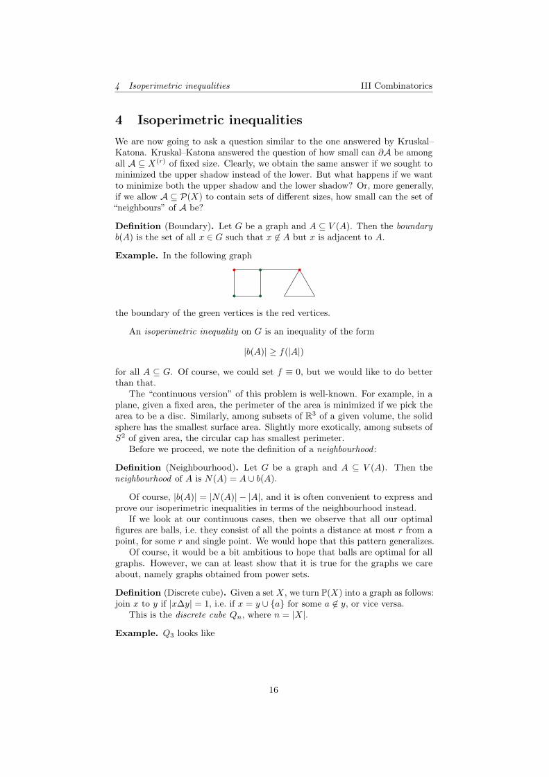
Example. In the following graph

the boundary of the green vertices is the red vertices.

An isoperimetric inequality on G is an inequality of the form

|b(A)| ≥ f(|A|)

for all A ⊆ G. Of course, we could set f ≡ 0, but we would like to do betterthan that.

The “continuous version” of this problem is well-known. For example, in aplane, given a fixed area, the perimeter of the area is minimized if we pick thearea to be a disc. Similarly, among subsets of R3 of a given volume, the solidsphere has the smallest surface area. Slightly more exotically, among subsets ofS2 of given area, the circular cap has smallest perimeter.

Before we proceed, we note the definition of a neighbourhood :

Definition (Neighbourhood). Let G be a graph and A ⊆ V (A). Then theneighbourhood of A is N(A) = A ∪ b(A).

Of course, |b(A)| = |N(A)| − |A|, and it is often convenient to express andprove our isoperimetric inequalities in terms of the neighbourhood instead.

If we look at our continuous cases, then we observe that all our optimalfigures are balls, i.e. they consist of all the points a distance at most r from apoint, for some r and single point. We would hope that this pattern generalizes.

Of course, it would be a bit ambitious to hope that balls are optimal for allgraphs. However, we can at least show that it is true for the graphs we careabout, namely graphs obtained from power sets.

Definition (Discrete cube). Given a set X, we turn P(X) into a graph as follows:join x to y if |x∆y| = 1, i.e. if x = y ∪ {a} for some a 6∈ y, or vice versa.

This is the discrete cube Qn, where n = |X|.

Example. Q3 looks like

16


123

1312 23

21 3

∅

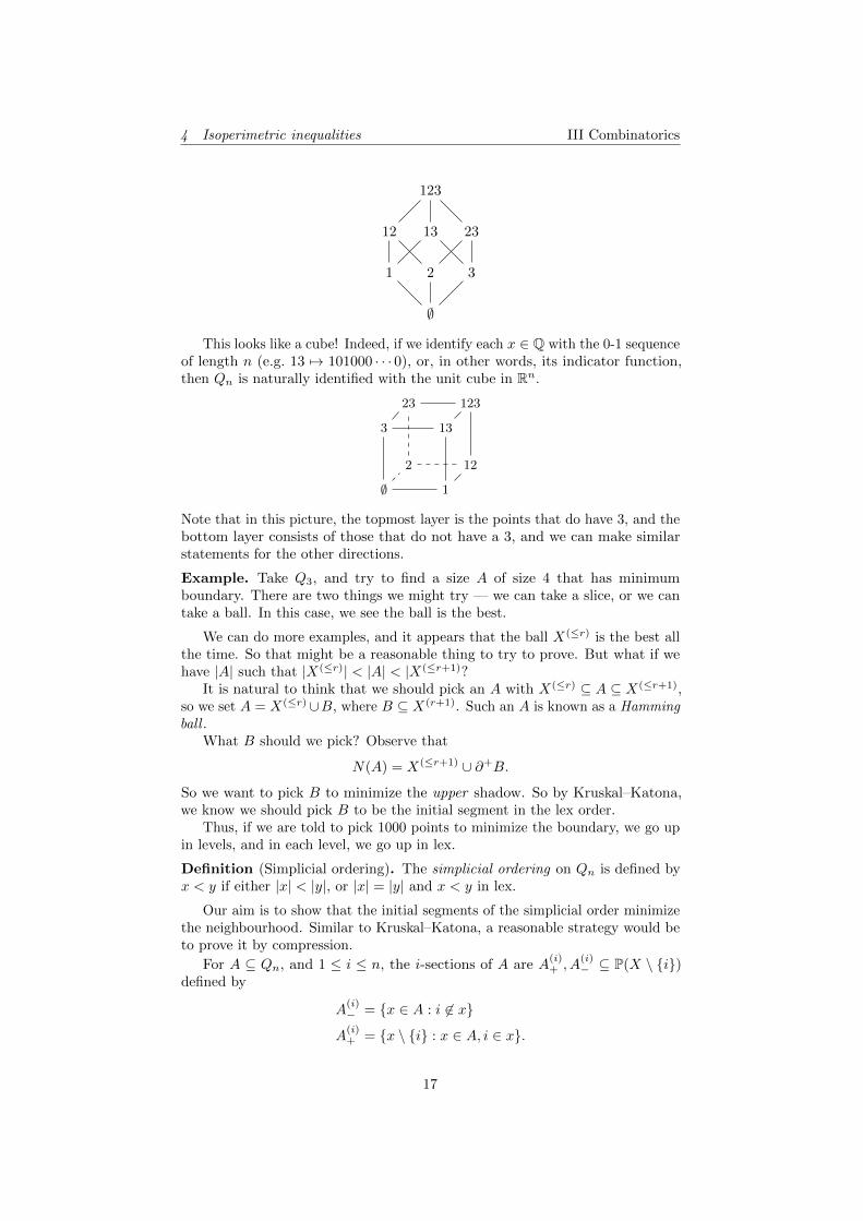
This looks like a cube! Indeed, if we identify each x ∈ Q with the 0-1 sequenceof length n (e.g. 13 7→ 101000 · · · 0), or, in other words, its indicator function,then Qn is naturally identified with the unit cube in Rn.

∅ 1

3

2 12

13

23 123

Note that in this picture, the topmost layer is the points that do have 3, and thebottom layer consists of those that do not have a 3, and we can make similarstatements for the other directions.

Example. Take Q3, and try to find a size A of size 4 that has minimumboundary. There are two things we might try — we can take a slice, or we cantake a ball. In this case, we see the ball is the best.

We can do more examples, and it appears that the ball X(≤r) is the best allthe time. So that might be a reasonable thing to try to prove. But what if wehave |A| such that |X(≤r)| < |A| < |X(≤r+1)?

It is natural to think that we should pick an A with X(≤r) ⊆ A ⊆ X(≤r+1),so we set A = X(≤r)∪B, where B ⊆ X(r+1). Such an A is known as a Hammingball .

What B should we pick? Observe that

N(A) = X(≤r+1) ∪ ∂+B.

So we want to pick B to minimize the upper shadow. So by Kruskal–Katona,we know we should pick B to be the initial segment in the lex order.

Thus, if we are told to pick 1000 points to minimize the boundary, we go upin levels, and in each level, we go up in lex.

Definition (Simplicial ordering). The simplicial ordering on Qn is defined byx < y if either |x| < |y|, or |x| = |y| and x < y in lex.

Our aim is to show that the initial segments of the simplicial order minimizethe neighbourhood. Similar to Kruskal–Katona, a reasonable strategy would beto prove it by compression.

For A ⊆ Qn, and 1 ≤ i ≤ n, the i-sections of A are A(i)+ , A

(i)− ⊆ P(X \ {i})

defined by

A(i)− = {x ∈ A : i 6∈ x}

A(i)+ = {x \ {i} : x ∈ A, i ∈ x}.

17


These are the top and bottom layers in the i direction.The i-compression (or co-dimension 1 compression) of A is Ci(A), defined by

Ci(A)+ = first |A+| elements of P(X \ {i}) in simplicial

Ci(A)− = first |A−| elements of P(X \ {i}) in simplicial

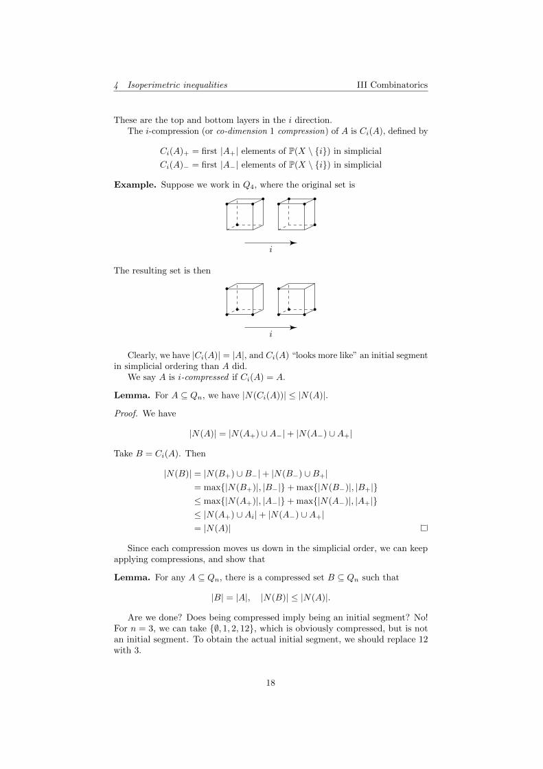
Example. Suppose we work in Q4, where the original set is

i

The resulting set is then

i

Clearly, we have |Ci(A)| = |A|, and Ci(A) “looks more like” an initial segmentin simplicial ordering than A did.

We say A is i-compressed if Ci(A) = A.

Lemma. For A ⊆ Qn, we have |N(Ci(A))| ≤ |N(A)|.

Proof. We have

|N(A)| = |N(A+) ∪A−|+ |N(A−) ∪A+|

Take B = Ci(A). Then

|N(B)| = |N(B+) ∪B−|+ |N(B−) ∪B+|= max{|N(B+)|, |B−|}+ max{|N(B−)|, |B+|}≤ max{|N(A+)|, |A−|}+ max{|N(A−)|, |A+|}≤ |N(A+) ∪Ai|+ |N(A−) ∪A+|= |N(A)|

Since each compression moves us down in the simplicial order, we can keepapplying compressions, and show that

Lemma. For any A ⊆ Qn, there is a compressed set B ⊆ Qn such that

|B| = |A|, |N(B)| ≤ |N(A)|.

Are we done? Does being compressed imply being an initial segment? No!For n = 3, we can take {∅, 1, 2, 12}, which is obviously compressed, but is notan initial segment. To obtain the actual initial segment, we should replace 12with 3.

18


∅ 1

3

2 12

13

23 123

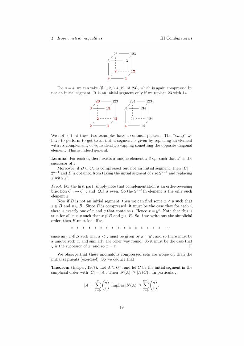
For n = 4, we can take {∅, 1, 2, 3, 4, 12, 13, 23}, which is again compressed bynot an initial segment. It is an initial segment only if we replace 23 with 14.

∅ 1

3

2 12

13

23 123

4 14

34

24 124

134

234 1234

We notice that these two examples have a common pattern. The “swap” wehave to perform to get to an initial segment is given by replacing an elementwith its complement, or equivalently, swapping something the opposite diagonalelement. This is indeed general.

Lemma. For each n, there exists a unique element z ∈ Qn such that zc is thesuccessor of z.

Moreover, if B ⊆ Qn is compressed but not an initial segment, then |B| =2n−1 and B is obtained from taking the initial segment of size 2n−1 and replacingx with xc.

Proof. For the first part, simply note that complementation is an order-reversingbijection Qn → Qn, and |Qn| is even. So the 2n−1th element is the only suchelement z.

Now if B is not an initial segment, then we can find some x < y such thatx 6∈ B and y ∈ B. Since B is compressed, it must be the case that for each i,there is exactly one of x and y that contains i. Hence x = yc. Note that this istrue for all x < y such that x 6∈ B and y ∈ B. So if we write out the simplicialorder, then B must look like

· · ·

since any x 6∈ B such that x < y must be given by x = yc, and so there must bea unique such x, and similarly the other way round. So it must be the case thaty is the successor of x, and so x = z.

We observe that these anomalous compressed sets are worse off than theinitial segments (exercise!). So we deduce that

Theorem (Harper, 1967). Let A ⊆ Qn, and let C be the initial segment in thesimplicial order with |C| = |A|. Then |N(A)| ≥ |N(C)|. In particular,

|A| =r∑

i=0

(n

i

)implies |N(A)| ≥

r+1∑i=0

(n

i

).

19


The edge isoperimetric inequality in the cube

Let A ⊆ V be a subset of vertices in a graph G = (V,E). Consider the edgeboundary

∂eA = {xy ∈ E : x ∈ A, y 6∈ A}.

Given a graph G, and given the size of A, can we give a lower bound for the sizeof ∂eA?

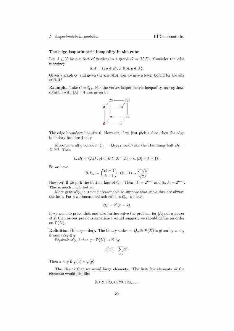
Example. Take G = Q3. For the vertex isoperimetric inequality, our optimalsolution with |A| = 4 was given by

∅ 1

3

2 12

13

23 123

The edge boundary has size 6. However, if we just pick a slice, then the edgeboundary has size 4 only.

More generally, consider Qn = Q2k+1, and take the Hamming ball Bk =X(≤`). Then

∂eBk = {AB : A ⊆ B ⊆ X : |A| = k, |B| = k + 1}.

So we have

|∂eBk| =(

2k + 1

k + 1

)· (k + 1) ∼ 2n

√n√

2π.

However, if we pick the bottom face of Qn. Then |A| = 2n−1 and |∂eA| = 2n−1.This is much much better.

More generally, it is not unreasonable to suppose that sub-cubes are alwaysthe best. For a k-dimensional sub-cube in Qn, we have

|∂k| = 2k(n− k).

If we want to prove this, and also further solve the problem for |A| not a powerof 2, then as our previous experience would suggest, we should define an orderon P(X).

Definition (Binary order). The binary order on Qn∼= P(X) is given by x < y

if maxx∆y ∈ y.Equivalently, define ϕ : P(X)→ N by

ϕ(x) =∑i∈x

2i.

Then x < y if ϕ(x) < ϕ(y).

The idea is that we avoid large elements. The first few elements in theelements would like like

∅, 1, 2, 123, 13, 23, 123, . . . .

20


Theorem. Let A ⊆ Qn be a subset, and let C ⊆ Qn be the initial segment oflength |A| in the binary order. Then |∂eC| ≤ |∂eA|.

Proof. We induct on n using codimension-1 compressions. Recall that we

previously defined the sets A(i)± .

The i-compression of A is the set B ⊆ Qn such that |B(i)± | = |A

(i)± |, and B

(i)±

are initial segments in the binary order. We set Di(A) = B.Observe that performing Di reduces the edge boundary. Indeed, given any

A, we have

|∂eA| = |∂eA(i)+ |+ |∂eA

(i)− |+ |A

(i)+ ∆A

(i)i |.

Applying Di clearly does not increase any of those factors. So we are happy.Now note that if A 6= DiA, then∑

x∈A

∑i∈x

2i <∑

x∈DiA

∑i∈x

2i.

So after applying compressions finitely many times, we are left with a compressedset.

We now hope that a compressed subset must be an initial segment, but thisis not quite true.

Claim. If A is compressed but not an initial, then

A = B = P(X \ {n}) \ {123 · · · (n− 1)} ∪ {n}.

By direct computation, we have

|∂eB| = 2n−1 − 2(n− 2),

and so the initial segment is better. So we are done.The proof of the claim is the same as last time. Indeed, by definition, we can

find some x < y such that x 6∈ A and y ∈ A. As before, for any i, it cannot bethe case that both x and y contain i or neither contain i, since A is compressed.So x = yc, and we are done as before.

21

5 Sum sets III Combinatorics

5 Sum sets

Let G be an abelian group, and A,B ⊆ G. Define

A+B = {a+ b : a ∈ A, b ∈ B}.

For example, suppose G = R and A = {a1 < a2 < · · · < an} and B = {b1 <b2 < · · · < bm}. Surely, A+B ≤ nm, and this bound can be achieved. Can webound it from below? The elements

a1 + b1, a1 + b2, . . . , a1 + bm, a2 + bm, . . . , an + bm

are certainly distinct as well, since they are in strictly increasing order. So

|A+B| ≥ m+ n− 1 = |A|+ |B| − 1.

What if we are working in a finite group? In general, we don’t have an order, sowe can’t make the same argument. Indeed, the same inequality cannot alwaysbe true, since |G+G| = |G|. Slightly more generally, if H is a subgroup of G,then |H +H| = |H|.

So let’s look at a group with no subgroups. In other words, pick G = Zp.

Theorem (Cauchy–Davenport theorem). Let A and B be non-empty subsetsof Zp with p a prime, and |A|+ |B| ≤ p+ 1. Then

|A+B| ≥ |A|+ |B| − 1.

Proof. We may assume 1 ≤ |A| ≤ |B|. Apply induction on |A|. If |A| = 1, thenthere is nothing to do. So assume A ≥ 2.

Since everything is invariant under translation, we may assume 0, a ∈ A witha 6= 0. Then {a, 2a, . . . , pa} = Zp. So there exists k ≥ 0 such that ka ∈ B and(k + 1)a 6∈ B.

By translating B, we may assume 0 ∈ B and a 6∈ B.Now 0 ∈ A ∩B, while a ∈ A \B. Therefore we have

1 ≤ |A ∩B| < |A|.

Hence

|(A ∩B) + (A ∪B)| ≥ |A ∩B|+ |A ∪B| − 1 = |A|+ |B| − 1.

Also, clearly(A ∩B) + (A ∪B) ⊆ A+B.

So we are done.

Corollary. Let A1, . . . , Ak be non-empty subsets of Zp such that

d∑i=1

|Ai| ≤ p+ k − 1.

Then

|A1 + . . .+Ak| ≥k∑

i=1

|Ai| − k + 1.

22

5 Sum sets III Combinatorics

What if we don’t take sets, but sequences? Let a1, . . . , am ∈ Zn. What mdo we need to take to guarantee that there are m elements that sums to 0? Bythe pigeonhole principle, m ≥ n suffices. Indeed, consider the sequence

a1, a1 + a2, a1 + a2 + a3, · · · , a1 + · · ·+ an.

If they are all distinct, then one of them must be zero, and so we are done. Ifthey are not distinct, then by the pigeonhole principle, there must be k < k′

such thata1 + · · ·+ ak = a1 + · · ·+ ak′ .

So it follows thatak+1 + · · ·+ ak′ .

So in fact we can even require the elements we sum over to be consecutive. Onthe other hand, m ≥ n is also necessary, since we can take ai = 1 for all i.

We can tackle a harder question, where we require that the sum of a fixednumber of things vanishes.

Theorem (Erdos–Ginzburg–Ziv). Let a1, . . . , a2n−1 ∈ Zn. Then there existsI ∈ [2n− 1](n) such that ∑

i∈Iai = 0

in Zn.

Proof. First consider the case n = p is a prime. Write

0 ≤ a1 ≤ a2 ≤ · · · ≤ a2p−1 < p.

If ai = ai+p−1, then there are p terms that are the same, and so we are doneby adding them up. Otherwise, set Ai = {ai, ai+p−1} for i = 1, . . . , p− 1, andAp = {a2p−1}, then |Ai| = 2 for i = 1, . . . , p− 1 and |Ap| = 1. Hence we know

|A1 + · · ·+Ap| ≥ (2(p− 1) + 1)− p+ 1 = p.

Thus, every element in Zp is a sum of some p of our terms, and in particular 0 is.In general, suppose n is not a prime. Write n = pm, where p is a prime and

m > 1. By induction, for every 2m− 1 terms, we can find m terms whose sumis a multiple of m.

Select disjoint S1, S2, . . . , S2p−1 ∈ [2n− 1](m) such that∑j∈Si

aj = mbi.

This can be done because after selecting, say, S1, . . . , S2p−2, we have

(2n− 1)− (2p− 2)m = 2m− 1

elements left, and so we can pick the next one.We are essentially done, because we can pick j1, . . . , jp such that

∑pk=1 bik is

a multiple of p. Thenp∑

k=1

∑j∈Sik

aj

is a sum of mp = n terms whose sum is a multiple of mp.

23

6 Projections III Combinatorics

6 Projections

So far, we have been considering discrete objects only. For a change, let’s workwith something continuous.

Let K ⊆ Rn be a bounded open set. For A ⊆ [n], we set

KA = {(xi)i∈A : ∃y ∈ K, yi − xi for all i ∈ A} ⊆ RA.

We write |KA| for the Lebesgue measure of KA as a subset of RA. The questionwe are interested in is given some of these |KA|, can we bound |K|? In somecases, it is completely trivial.

Example. If we have a partition of A1 ∪ · · · ∪Am = [n], then we have

|K| ≤m∏i=1

|KAi |.

But, for example, in R3, can we bound |K| given |K12|, |K13| and |K23|?It is clearly not possible if we only know, say |K12| and |K13|. For example,

we can consider the boxes (0,

1

n

)× (0, n)× (0, n).

Proposition. Let K be a body in R3. Then

|K|2 ≤ |K12||K13||K23|.

This is actually quite hard to prove! However, given what we have done sofar, it is natural to try to compress K in some sense. Indeed, we know equalityholds for a box, and if we can make K look more like a box, then maybe we canend up with a proof.

For K ⊆ Rn, its n-sections are the sets K(x) ⊆ Rn−1 defined by

K(x) = {(x1, . . . , xn−1) ∈ Rn−1 : (x1, . . . , xn−1, x) ∈ K}.

Proof. Suppose first that each section of K is a square, i.e.

K(x) = (0, f(x))× (0, f(x)) dx

for all x and some f . Then

|K| =∫f(x)2 dx.

Moreover,

|K12| =(

supxf(x)

)2

≡M2, |K13| = |K23| =∫f(x) dx.

So we have to show that(∫f(x)2 dx

)2

≤M2

(∫f(x) dx

)2

,

24


but this is trivial, because f(x) ≤M for all x.Let’s now consider what happens when we compress K. For the general case,

define a new body L ⊆ R3 by setting its sections to be

L(x) = (0,√|K(x)|)× (0,

√|K(x)|).

Then |L| = |K|, and observe that

|L12| ≤ sup |K(x)| ≤∣∣∣⋃K(x)

∣∣∣ = |K12|.

To understand the other two projections, we introduce

g(x) = |K(x)1|, h(x) = |K(x)2|.

Now observe that|L(x)| = |K(x)| ≤ g(x)h(x),

Since L(x) is a square, it follows that L(x) has side length ≤ g(x)1/2h(x)1/2. So

|L13| = |L23| ≤∫g(x)1/2h(x)1/2 dx.

So we want to show that(∫g1/2h1/2 dx

)2

≤(∫

g dx

)(∫h dx

).

Observe that this is just the Cauchy–Schwarz inequality applied to g1/2 andh1/2. So we are done.

Let’s try to generalize this.

Definition ((Uniform) cover). We say a family A1, . . . , Ar ⊆ [n] covers [n] if

r⋃i=1

Ar = [n],

and is a uniform k-cover if each i ∈ [n] is in exactly k many of the sets.

Example. With n = 3, the singletons {1}, {2}, {3} form a 1-uniform cover,and so does {1}, {2, 3}. Also, {1, 2}, {1, 3} and {2, 3} form a uniform 2-cover.However, {1, 2} and {2, 3} do not form a uniform cover of [3].

Note that we allow repetitions.

Example. {1}, {1}, {2, 3}, {2}, {3} is a 2-uniform cover of [3].

Theorem (Uniform cover inequality). If A1, . . . , Ar is a uniform k-cover of [n],then

|K|k =

r∏i=1

|KA|.

25


Proof. Let A be a k-uniform cover of [k]. Note that A is a multiset. Write

A− = {A ∈ A : n 6∈ A}A+ = {A \ {n} ∈ A : n ∈ A}

We have |A+| = k, and A+ ∪ A− forms a k-uniform cover of [n− 1].Now note that if K = Rn and n 6∈ A, then

|KA| ≥ |K(x)A| (1)

for all x. Also, if n ∈ A, then

|KA| =∫|K(x)A\{n}| dx. (2)

In the previous proof, we used Cauchy–Schwarz. What we need here is Holder’sinequality ∫

fg dx ≤(∫

fp dx

)1/p(∫gq dx

)1/q

,

where 1p + 1

q = 1. Iterating this, we get

∫f1 · · · fk dx ≤

k∏i=1

(∫fki dx

)1/k

.

Now to perform the proof, we induct on n. We are done if n = 1. Otherwise,given K ⊆ Rn and n ≥ 2, by induction,

|K| =∫|K(x)| dx

≤∫ ∏

A∈A−

|K(x)A|1/k∏

A∈A+

|K(x)A|1/k dx (by induction)

≤∏

A∈A−

|KA|1/k∫ ∏

A∈A+

|K(x)A|1/k dx (by (1))

≤∏

A≤|A−

|KA|1/k∏

A∈A+

(∫|K(x)A|

)1/k

(by Holder)

=∏A∈A|KA|1/k

∏A∈A+

|KA∪{n}|1/k. (by (2))

This theorem is great, but we can do better. In fact,

Theorem (Box Theorem (Bollobas, Thomason)). Given a body K ⊆ Rn, i.e.a non-empty bounded open set, there exists a box L such that |L| = |K| and|LA| ≤ |KA| for all A ⊆ [n].

Of course, this trivially implies the uniform cover theorem. Perhaps moresurprisingly, we can deduce this from the uniform cover inequality.

To prove this, we first need a lemma.

26


Definition (Irreducible cover). A uniform k-cover is reducible if it is the disjointunion of two uniform covers. Otherwise, it is irreducible.

Lemma. There are only finitely many irreducible covers of [n].

Proof. Let A and B be covers. We say A < B if A is a “subset” of B, i.e. foreach A ⊆ [n], the multiplicity of A in A is less than the multiplicity in B.

Then note that the set of irreducible uniform k-covers form an anti-chain,and observe that there cannot be an infinite anti-chain.

Proof of box theorem. For A an irreducible cover, we have

|K|k ≤∏A∈A|KA|.

Also,

|KA| ≤∏i∈A|K{i}|.

Let {xA : A ⊆ [n]} be a minimal array with xA ≤ |KA| such that for eachirreducible k-cover A, we have

|K|k ≤∏A∈A

xA (1)

and moreoverxA ≤

∏i∈A

x{i} (2)

for all A ⊆ [n]. We know this exists since there are only finitely many inequalitiesto be satisfied, and we can just decrease the xA’s one by one. Now again byfiniteness, for each xA, there must be at least one inequality involving xA on theright-hand side that is in fact an equality.

Claim. For each i ∈ [n], there exists a uniform ki-cover Ci containing {i} withequality

|K|ki =∏A∈Ci

xA.

Indeed if xi occurs on the right of (1), then we are done. Otherwise, it occurson the right of (2), and then there is some A such that (2) holds with equality.Now there is some cover A containing A such that (1) holds with equality. Thenreplace A in A with {{j} : j ∈ A}, and we are done.

Now let

C =

n⋃i=1

Ci, C′ = C \ {{1}, {2}, . . . , {n}}, k =

n∑i=1

ki.

Then

|K|k =∏A∈C

xA =

( ∏A∈C1

xA

)≥ |K|k−1

n∏i=1

xi.

27


So we have

|K| ≥n∏

i=1

xi.

But we of course also have the reverse inequality. So it must be the case thatthey are equal.

Finally, for each A, consider A = {A} ∪ {{i} : i 6∈ A}. Then dividing (1) by∏i∈A xi gives us ∏

i 6∈A

xi ≤ xA.

By (2), we have the inverse equality. So we have

xA =∏i∈A

xi

for all i. So we are done by taking L to be the box with side length xi.

Corollary. If K is a union of translates of the unit cube, then for any (notnecessarily uniform) k-cover A, we have

|K|k ≤∏A∈A|KA|.

Here a k-cover is a cover where every element is covered at least k times.

Proof. Observe that if B ⊆ A, then |KB | ≤ |KA|. So we can reduce A to auniform k-cover.

28

7 Alon’s combinatorial Nullstellensatz III Combinatorics

7 Alon’s combinatorial Nullstellensatz

Alon’s combinatorial Nullstellensatz is a seemingly unexciting result that hassurprisingly many useful consequences.

Theorem (Alon’s combinatorial Nullstellensatz). Let F be a field, and letS1, . . . , Sn be non-empty finite subsets of F with |Si| = di + 1. Let f ∈F[X1, . . . , Xn] have degree d =

∑ni=1 di, and let the coefficient of Xd1

1 · · ·Xdnn be

non-zero. Then f is not identically zero on S = S1 × · · · × Sn.

Its proof follows from generalizing facts we know about polynomials in onevariable. Here R will always be a ring; F always a field, and Fq the unique fieldof order q = pn. Recall the following result:

Proposition (Division algorithm). Let f, g ∈ R[X] with g monic. Then we canwrite

f = hg + r,

where deg h ≤ deg f − deg g and deg r < deg g.

Our convention is that deg 0 = −∞.Let X = (X1, . . . , Xn) be a sequence of variables, and write R[X] =

R[X1, . . . , Xn].

Lemma. Let f ∈ R[X], and for i = 1, . . . , n, let gi(Xi) ∈ R[Xi] ⊆ R[X]be monic of degree deg gi = degXi

gi = di. Then there exists polynomialsh1, . . . , hn, r ∈ R[X] such that

f =∑

figi + r,

where

deg hi ≤ deg f − deg di degXir ≤ di − 1

degXihi ≤ degXi

f − di degXir ≤ degXi

f

degXjhi ≤ degXj

f deg r ≤ deg f

for all i, j.

Proof. Consider f as a polynomial with coefficients in R[X2, . . . , Xn], then divideby g1 using the division algorithm. So we write

f = h1g1 + r1.

Then we have

degX1h1 ≤ degX1

f − d1 degX1r1 ≤ d1 − 1

deg h1 ≤ deg f degXjr1 ≤ degXj

f

degXjh1 ≤ degXj

f deg r ≤ deg f.

Then repeat this with f replaced by r1, g1 by g2, and X1 by X2.

We also know that a polynomial of one variable of degree n ≥ 1 over a fieldhas at most n zeroes.

29


Lemma. Let S1, . . . , Sn be non-empty finite subsets of a field F, and let h ∈ F[X]be such that degXi

h < |Si| for i = 1, . . . , n. Suppose h is identically 0 onS = S1 × · · · × Sn ⊆ Fn. Then h is the zero polynomial.

Proof. Let di = |Si| − 1. We induct on n. If n = 1, then we are done. For n ≥ 2,consider h as a one-variable polynomial in F [X1, . . . , Xn−1] in Xn. Then we canwrite

h =

dn∑i=0

gi(X1, . . . , Xn−1)Xim.

Fix (x1, . . . , xn−1) ∈ S1 × · · ·Sn−1, and set ci = gi(x1, . . . , xn−1) ∈ F. Then∑dn

i=0 ciXin vanishes on Sn. So ci = gi(x1, . . . , xn−1) = 0 for all (x1, . . . , xn−1) ∈

S1 × · · · × Sn−1. So by induction, gi = 0. So h = 0.

Another fact we know about polynomials in one variables is that if f ∈ F[X]vanishes at z1, . . . , zn, then f is a multiple of

∏ni=1(X − zi).

Lemma. For i = 1, . . . , n, let Si be a non-empty finite subset of F, and let

gi(Xi) =∏s∈Si

(Xi − s) ∈ F[Xi] ⊆ F [X].

Then if f ∈ F[X] is identically zero on S = S1 × · · · × Sn, then there existshi ∈ F[X], deg hi ≤ deg f − |Si| and

f =

n∑i=1

higi.

Proof. By the division algorithm, we can write

f =

n∑i=1

higi + r,

where r satisfies degXir < deg gi. But then r vanishes on S1 × · · · × Sn, as both

f and gi do. So r = 0.

We finally get to Alon’s combinatorial Nullstellensatz.

Theorem (Alon’s combinatorial Nullstellensatz). Let S1, . . . , Sn be non-emptyfinite subsets of F with |Si| = di + 1. Let f ∈ F[X] have degree d =

∑ni=1 di,

and let the coefficient of Xd11 · · ·Xdn

n be non-zero. Then f is not identically zeroon S = S1 × · · · × Sn.

Proof. Suppose for contradiction that f is identically zero on S. Define gi(Xi)and hi as before such that

f =∑

higi.

Since the coefficient of Xd11 · · ·Xdn

n is non-zero in f , it is non-zero in some hjgj .But that’s impossible, since

deg hj ≤

(n∑

i=1

di

)− deg gj =

∑i 6=j

di − 1,

and so hj cannot contain a Xd11 · · · Xj

dj · · ·Xdnn term.

30


Let’s look at some applications. Here p is a prime, q = pk, and Fq is theunique field of order q.

Theorem (Chevalley, 1935). Let f1, . . . , fm ∈ Fq[X1, . . . , Xn] be such that

m∑i=1

deg fi < n.

Then the fi cannot have exactly one common zero.

Proof. Suppose not. We may assume that the common zero is 0 = (0, . . . , 0).Define

f =

m∏i=1

(1− fi(X)q−1)− γn∏

i=1

∏s∈F×q

(Xi − s),

where γ is chosen so that F (0) = 0, namely the inverse of(∏

s∈F×q (−s))m

.

Now observe that for any non-zero x, the value of fi(x)q−1 = 1, so f(x) = 0.Thus, we can set Si = Fq, and they satisfy the hypothesis of the theorem. In

particular, the coefficient of Xq−11 · · ·Xq−1

n is γ 6= 0. However, f vanishes on Fnq .

This is a contradiction.

It is possible to prove similar results without using the combinatorial Null-stellensatz. These results are often collectively refered to as Chevalley–Warningtheorems.

Theorem (Warning). Let f(X) = f(X1, . . . , Xn) ∈ Fq[X] have degree < n.Then N(f), the number of zeroes of f is a multiple of p.

One nice trick in doing these things is that finite fields naturally come withan “indicator function”. Since the multiplicative group has order q− 1, we knowthat if x ∈ Fq, then

xq−1 =

{1 x 6= 0

0 x = 0.

Proof. We have

1− f(x)q−1 =

{1 f(x) = 0

0 otherwise.

Thus, we know

N(f) =∑x∈Fn

q

(1− f(x)q−1) = −∑x∈Fn

q

f(x)q−1 ∈ Fq.

Further, we know that if k ≥ 0, then

∑x∈Fn

q

xk =

{−1 k = q − 1

0 otherwise.

So let’s write f(x)q−1 as a linear combination of monomials. Each monomialhas degree < n(q − 1). So there is at least one k such that the power of Xk inthat monomial is < q − 1. Then the sum over Xk vanishes for this monomial.So each monomial contributes 0 to the sum.

31


We can use Alon’s combinatorial Nullstellensatz to effortlessly prove some ofour previous theorems.

Theorem (Cauchy–Davenport theorem). Let p be a prime and A,B ⊆ Zp benon-empty subsets with |A|+ |B| ≤ p+ 1. Then |A+B| ≥ |A|+ |B| − 1.

Proof. Suppose for contradiction that A+B ⊆ C ⊆ Zp, and |C| = |A|+ |B| − 2.Let’s come up with a polynomial that encodes the fact that C contains the sumA+B. We let

f(X,Y ) =∏c∈C

(X + Y − c).

Then f vanishes on A×B, and deg f = |C|.To apply the theorem, we check that the coefficient of X |A|−1Y |B|−1 is

( |C||A|−1

),

which is non-zero in Zp, since C < p. This contradicts Alon’s combinatorialNullstellensatz.

We can also use this to prove Erdos–Ginzburg–Ziv again.

Theorem (Erdos–Ginzburg–Ziv). Let p be a prime and a1, . . . , a2p+1 ∈ Zp.Then there exists I ∈ [2p− 1](p) such that∑

i∈Iai = 0 ∈ Zp.

Proof. Define

f1(X1, . . . , X2p−1) =

2p−1∑i=1

Xp−1i .

f2(X1, . . . , X2p−1) =

2p−1∑i=1

aiXp−1i .

Then by Chevalley’s theorem, we know there cannot be exactly one commonzero. But 0 is one common zero. So there must be another. Take this solution,and let I = {i : xi 6= 0}. Then f1(X) = 0 is the same as saying |I| = p, andf2(X) = 0 is the same as saying

∑i∈I ai = 0.

We can also consider restricted sums. We set

A·+B = {a+ b : a ∈ A, b ∈ B, a 6= b}.

Example. If n 6= m, then

[n]·+ [m] = {3, 4, . . . ,m+ n}

[n]·+ [n] = {3, 4, . . . , 2n− 1}

From this example, we show that if |A| ≥ 2, then |A·+A| can be as small as

2|A| − 3. In 1964, Erdos and Heilbronn

Conjecture (Erdos–Heilbronn, 1964). If 2|A| ≤ p+ 3, then |A·+A| ≥ 2|A| − 3.

32


This remained open for 30 years, and was proved by Dias da Silva andHamidoune. A much much simpler proof was given by Alon, Nathanson andRuzsa in 1996.

Theorem. Let A,B ⊆ Zp be such that 2 ≤ |A| < |B| and |A| + |B| ≤ p + 2.

Then A·+B ≥ |A|+ |B| − 2.

The above example shows we cannot do better.

Proof. Suppose not. Define

f(X,Y ) = (X − Y )∏c∈C

(X + Y − c),

where A·+B ⊆ C ⊆ Zp and |C| = |A|+ |B| − 3.

Then deg g = |A|+ |B| − 2, and the coefficient of X |A|−1Y |B|−1 is(|A|+ |B| − 3

|A| − 2

)−(|A|+ |B| − 3

|A| − 1

)6= 0.

Hence by Alon’s combinatorial Nullstellensatz, f(x, y) is not identically zero onA×B. A contradiction.

Corollary (Erdos–Heilbronn conjecture). If A,B ⊆ Zp, non-empty and |A|+|B| ≤ p+ 3, and p is a prime, then |A

·+B| ≥ |A|+ |B| − 3.

Proof. We may assume 2 ≤ |A| ≤ |B|. Pick a ∈ A, and set A′ = A \ {a}. Then

|A·+B| ≥ |A′

·+B| ≥ |A′|+ |B| − 2 = |A|+ |B| − 3.

Now consider the following problem: suppose we have a circular table Z2n+1.Suppose the host invites n couples, and the host, being a terrible person, wantsthe ith couple to be a disatnce di apart for some 1 ≤ di ≤ n. Can this be done?

Theorem. If 2n+ 1 is a prime, then this can be done.

Proof. We may wlog assume the host is at 0. We want to partition Zp \{0} = Z×pinto n pairs {xi, xi + di}. Consider the polynomial ring Zp[X1, . . . , Xn] = Zp[X].We define

f(x) =∏i

Xi(Xi+di)∏i<j

(Xi−Xj)(Xi+di−Xj)(Xi−Xj−dj)(Xi+di−Xj−dj).

We want to show this is not identically zero on Znp

First of all, we have

deg f = 4

(n

2

)+ 2n = 2n2.

So we are good. The coefficient of X2n1 · · ·X2n

n is the same as that in

∏X2

i

∏i<j

(Xi −Xj)4 =

∏X2

i

∏i6=j

(Xi −Xj)2 =

∏X2n

i

∏i6=j

(1− Xi

Xj

)2

.

33


This, we are looking for the constant term in

∏i6=j

(1− Xi

Xj

)2

.

By a question on the example sheet, this is(2n

2, 2, . . . , 2

)6= 0 in Zp.

Our final example is as follows: suppose we are in Zp, and a1, . . . , ap andc1, . . . , cp are enumerations of the elements, and bi = ci − ai. Then clearly wehave

∑bi = 0. Is the converse true? The answer is yes!

Theorem. If b1, . . . , bp ∈ Zp are such that∑bi = 0, then there exists numer-

ations a1, . . . , ap and b1, . . . , bp of the elements of Zp such that for each i, wehave

ai + bi = ci.

Proof. It suffices to show that for all (bi), there are distinct a1, · · · , ap−1 suchthat ai + bi 6= aj + bj for all i 6= j. Consider the polynomial∏

i<j

(Xi −Xj)(Xi + bi −Xj − bj).

The degree is

2

(p− 1

2

)= (p− 1)(p− 2).

We then inspect the coefficient of Xp−21 · · ·Xp−2

p−1 , and checking that this isnon-zero is the same as above.

34

Index III Combinatorics

Index

(k, `)-regular, 3X(≤r), 5X(r), 5X≥r, 5Γ(S), 3P(X), 6·+, 32n-sections, 24

Alon’s combinatorialNullstellensatz, 29, 30

anti-chain, 6

ballHamming, 17

binary order, 20bipartite graph, 3biregular graph, 3boundary, 16box theorem, 26

Cauchy–Davenport theorem, 22, 32chain, 6Chevalley–Warning theorems, 31co-dimension 1 compression, 18colex order, 12combinatorial Nullstellensatz, 29,

30complete matching, 3compression operator, 11cover, 25

discrete cube, 16distinct representatives, 4division algorithm, 29

downward-expanding poset, 7

edge boundary, 20expanding, 7

graded poset, 6

Hall’s condition, 3Hall’s theorem, 3Hamming ball, 17

irreducible cover, 27isoperimetric inequality, 16

lex order, 12LYM inequality, 7

neighbourhood, 16

posetregular, 8

power set, 6

reducible cover, 27regular poset, 8restricted sum, 32

shadow, 7shadow function, 13simplicial ordering, 17symmetric chain, 9

uniform cover, 25uniform cover inequality, 25upward-expanding, 7

weight, 7

35

Documents

Part III - Combinatorics1 Hall’s theorem III Combinatorics 1 Hall’s theorem We shall begin with a discussion of Hall’s theorem. Ideally, you’ve already met it in IID Graph