Embed Size (px)
Citation preview
Pergamon Computers & Geosciences Vol. 20, No. 2, pp. 91-104, 1994
Copyright © 1994 Elsevier Science Ltd 0 0 9 8 - 3 0 0 4 ( 9 3 ) E 0 0 0 1 - V Printed in Great Britain. All rights reserved
0098-3004/94 $7.00 + 0.00
PARALLEL PROCESSING OF SPATIAL STATISTICS
MARC P. ARMSTRONG, l CLAIRE E. PAVLIK 2, and RICHARD MARCIANO 3 tDepartments of Geography and Computer Science, and Program in Applied Mathematical and
Computational Sciences, 2Department of Geography and 3Gerard P. Weeg Computer Center and Department of Computer Science, The University of Iowa, Iowa City, IA 52242, U.S.A.
(Received 12 March 1993; accepted 29 September 1993)
Abstract--The computational intensity of spatial statistics, including measures of spatial association, has hindered their application to large empirical data sets. Computing environments using parallel processing have the potential to eliminate this problem. In this paper, we develop a method for processing a computationally intensive measure of spatial association (G) in parallel and present the performance enhancements obtained. Timing results are presented for a single processor and for 2-14 parallel processors operating on data sets containing 256-1600 point observations. The results indicate that significant improvements in processing time can be achieved using parallel architectures.
Key Words: Parallel processing, Spatial statistics.
INTRODUCTION
The measurement of the strength and significance of spatial association for a collection of observations is important in a wide variety of research contexts. Anselin and Griffith (1988) for example demonstrate the importance of spatial effects on regression models that use spatial variables, whereas Oliver, Webster, and Gerard (1989a, 1989b) illustrate the use of semi- variance analysis to study and model spatial structure in soils and other types of physical data. Conse- quently, a variety of statistical evaluation techniques have been developed during the past several decades; many of these are based on autocorrelation measures (Cliff and Ord, 1981). Recently, Getis and Ord (1992) again have demonstrated that researchers must account for autocorrelation effects in spatial models and have presented a new method (G) to measure the degree of spatial association among point-referenced observations. Such measures have broad applications across the geosciences.
Measures of spatial association may require sub- stantial amounts of computation time because the amount of calculation tends to increase with the square of the problem size. For point data, such measures typically rely on interpoint distances, each of which requires the use of comparatively slow calculations (e.g. calculating Euclidean distance by squaring, summing, then taking the square root of differences in Cartesian coordinates). These aspects of geoprocessing have led, in part, to its relative marginalization with respect to the mainstream of statistical and analytical computing, despite the im- portance of these methods to the development of valid and accurate spatial models (Griffith, 1990). In
91
addition, the sheer size and computational load of real geographical computing problems have tended to preclude interactive, exploratory analyses of spatial data. As a result, several researchers (e.g. Griffith, 1990; Openshaw, Cross, and Charlton, 1990; Sandhu and Marble, 1988) have begun to explore the use of high-performance vector architectures to tackle geoprocessing problems.
"Traditional" high-performance vector processing architectures, which developed rapidly in the 1970s and 1980s, usually are characterized by high acqui- sition and maintenance costs. As a result of these costs high-performance computers have tended to be scarce, inaccessible resources. Although the technical development of these vector environments has been impressive, incremental performance enhancements now demonstrate decreasing returns on investment. Thus, as improvements continue to be wrested from these architectures, the cost of marginal increases in performance spirals upward and designers have looked to other architectures as potential candidates for high-performance computing. Computer manu- facturers and the research community have begun recently to exploit parallel processing architectures to provide cost-effective high performance computing environments (see e.g. Myers, 1993). Although paral- lel processing has been suggested as a way to over- come computational problems associated with the analysis of geographical data sets (e.g. Armstrong and Densham, 1992; Mills, Fox, and Heimbach, 1992), many experts in geoprocessing are unfamiliar with the task of converting a serial algorithm into a parallel implementation. The purpose of this paper is to illustrate this process of serial to parallel conver- sion for a computationally intensive algorithm and to
92 M.P. ARMSTRONG, C. E. PAVL1K, and R. MARCIANO
evaluate its performance across a range of problem sizes using different numbers of processors running in parallel.
BACKGROUND: PARALLEL PROCESSING
Parallel processing has a relatively long history in modern computing but, until recently, it has been of more interest as a research vehicle than as a practical approach to computational problem- solving. Language constructs for parallel processing such as fork and join were introduced by Conway (1963) and Dennis and Van Horn (1966). These were among the first language notations for specifying concurrency and preceded the com- mercial availability of parallel machines. A higher level language construct for specifying concurrency was the parbegin/parend statement of Dijkstra (1968).
In a widely used classification of computer archi- tectures (Flynn, 1966), two of the four main classes are parallel architectures. [For a complete description of these architectures, refer to Lilja (1991).] Parallel architectures defined as single instruction, multiple data stream (SIMD) computers use large numbers of simple processors to complete tasks, whereas those categorized as multiple instruction, multiple data (MIMD) computers typically have comparatively complex processing elements. Although both cat- egories are defined as parallel computers, individually and taken together they encompass a wide variety of processing elements and programming environ- ments. This diversity explains, in part, why the development of parallel processing has been slow: the range of architectures and the difficulty in moving between them has made these machines exotic. Specialized code to exploit the characteristics of each architecture had to be written. As a result, parallel code has lacked portability between environ- ments.
At present, a consensus on the constructs needed in parallel programming environments is developing. Just as programming languages for sequential ma- chines were codified and incrementally extended to enhance portability among computing environments, basic concepts required for parallel programming now are being identified and formalized. Thus the way in which these constructs are implemented is not necessarily identical for different machines, the underlying concepts are congruent. On some ma- chines, parallel programming extensions to existing languages ease the investment required to convert serial to parallel code. For example, the results presented in this paper were obtained using parallel extensions of FORTRAN in a MIMD computing environment. Although the specific dialect of FOR- TRAN used is not available universally, the general constructs used to implement the algorithm in paral- lel are adaptable readily to a broad class of parallel
architectures. Thus, the code itself is not directly portable, but it can be implemented easily on other parallel computing systems.
Compilers that purport to perform automated parallelization of conventional serial code have been developed; however, they have not been effective fully in capturing relationships that can be exploited by parallel architectures (e.g. Hwang and DeGroot, 1989; Pancake, 1991; Shen, Li, and Yew, 1990). While this shortcoming has been a tremendous boon to legions of computer science graduate students, it is incumbent upon researchers to become familiar with the parallelization process as it will be a routine part of computing practices. Because serial architectures have been the dominant computing environments, most algorithms have been developed and optimized for these architectures. In order to take advantage of the performance capabilities of parallel architectures, serial algorithms must be converted to exploit their inherent parallelism; thus, the conversion of algorithms from serial to parallel versions will become commonplace during the 1990s.
BACKGROUND: G STATISTICS
The statistic selected to illustrate the serial-to-par- allel conversion process is from a family of statistics known as G (Getis and Ord, 1992). The specific form of the G statistic used here [G(d)] measures the spatial assocation of point-referenced data in the plane. Unlike other well-known measures such as Moran's I or Geary's c (Cliff and Ord, 1981), G(d) does not provide a global assessment of spatial structure, but focuses on local structure. Normally the statistic is reported as a series of measures calculated for a set of user-specified distances. Getis and Ord (1992) state that this local focus is important especially if spatial data have unequal local averages and values that are related by the distance between observations rather than by absolute location. These characteristics, also known as "nonstationarity", usually occur in spatial data collections (Cliff and Ord, 1981; Oliver, Webster, and Gerrard, 1989a).
Let us define the data set as n observations, labeled as sites 1 to n, each described by Cartesian coordi- nates and a positive, real-valued variable, x. The G(d) statistic focuses on spatial association by summar- izing characteristics of the x-values contained in circles of differing sizes. The procedure is summarized easily: imagine a set of observations assigned to points on a two-dimensional (2-D) surface. Select a single point, site i, and center a circle of radius d on it. Compute the product of site i's x-value with the x-value for each of the other sites within the circle, then sum these products. Repeat the procedure for the rest of the sites with the same radius circle, then add the summed values for all sites. Finally, normal- ize this result by dividing it by the double-sum of all
Parallel processing of spatial statistics 93
different site xixj-products. Stated in equation form, the G(d) statistic is:
n
E wi,(d)x,x, G ( d ) : i= l ]=l
iixi , i = l j - I
j not equal to i, Vi = 1 . . . . . j = 1 . . . . . n, (1)
where the ~% (d) are binary variables that indicate whether site j is within radius d of site i (w o ( d ) = 1) or not (w 0 ( d ) = 0).
Using this equation, a series of statistics that evaluate G for circles of various radii can be com- puted. These statistics are used to determine the degree of spatial association through comparison to expected values under the assumption of no spatial association. Because the expected value and variance of the statistic can be computed, G-statistics also may be standardized for comparison across data sets; standardized G (d) values for individual sites may be compared as well (see Getis and Ord, 1992). The expected value of the statistic is defined by:
where
E[G(d)I = W/[n (n -- 1)], (2)
w = E Y w,j(d), i = l j = l
j not equal to i, Vi = 1 , . . . ,n, j = 1 . . . . . n. Calculation of G(d) is intensive computationally
for two reasons. First, similar to many other measures of spatial association, it requires the com- putation of interpoint distances among observations, and computation of these distances increases as the square of the problem size. Moreover, distance com- putations by themselves require a substantial amount of calculation. Depending on the instruction set of the computer used, the execution of multiplications and square roots may take several cycles to produce a single result. Because each of these operations is performed repeatedly by the program, computation increases rapidly with problem size. Similar problems have been reported by other researchers who have examined distance-related computations. MacDou- gall (1984), for example, has demonstrated the effect of problem size on the computation times required for interpolating inverse distance weighted surfaces on a microcomputer.
The second cause of computational burden lies in the way the G(d) selects points to be used in the calculation of the statistic. In the heuristic used to describe the statistic, we can imagine performing calculations only for observations that fall in a circle of a certain radius; for machine computation, how- ever, the selection of points for the calculation is not performed by visual inspection, but by comparison of the distance between two observations with a radius cutoff value. Depending on the structure of the algorithm used, the calculation of G(d) for a series of
d-values may involve examining an entire matrix of interpoint distances, and performing some calcu- lations only for those observations with interpoint distances less than d.
PARALLEL IMPLEMENTATION OF G(d)
To implement a parallel version of a program originally formulated for serial implementation, a programmer must make several decisions that are conditioned by the architecture of the parallel com- puter and the structure of the algorithm. First, the sequential program must be divided into parts that will be executed concurrently on the parallel com- puter. For SIMD computers, the size of these units usually is small (e.g. instruction level), whereas there is considerably more flexibility in the size of the subproblem that can be allocated to each processor on MIMD computers. It is usual, for example, to place several different portions of a loop on different MIMD processing elements (PE), each of which are given different portions of data to execute. In parti- tioning the program, the size of the set of instructions allocated to each of the parallel processors is referred to as its granularity. In the implementation described here, we adopted a relatively coarse-grained ap- proach to program partitioning. This is in keeping with the characteristics of the MIMD computer used.
The parallel computing environment
The program was written for an Encore Multimax. The Multimax is a modular, expandable multiproces- sor system built around the Nanobus, a wide, fast (sustained bandwidth of 100 MB/sec) bus that pro- vides the primary communications pathway among system modules (ANL, 1987). A Multimax system incorporates from 2 to 20 32-bit processors, each provided with a 32KB cache of fast static RAM, and from 4 to 32 MB of fast shared memory. The Encore Multimax (Encore Computer Corp., 1988) used in the computing experiments described in this paper was configured as follows:
• 14 NS32332 processors (3 MIPS/processor for a total of 42 MIPS) and
• 32 MB of shared memory.
Language extensions to accommodate parallel con- s l r u c l s
Programming in parallel environments usually is supported by a set of extensions to conventional languages. Carriero and Gelernter (1990) for example describe a "dual language" approach to parallel programming in which a programmer uses a comput- ing language, such as FORTRAN, to calculate and perform data manipulation tasks, and a specialized coordination language to create parallel processes and support communication among them. The three
94 M.P. ARMSTRONG, C. E. PAVLIK, and R. MARCIANO
major constructs that may be supported by parallel extensions to programming languages are:
• Process creation: mechanisms must be pro- vided for creating multiple "execution units" that have separate existence and can be executed in parallel.
• Sharing or privatization of memory: parallel pro- cesses may need to share data that are common to the problem being solved.
• Process synchronization: synchronization mech- anisms allow parallel processes to access shared data in a controlled and orderly fashion.
Encore Parallel FORTRAN (EPF)
Our parallel implementation of G(d) uses the En- core Parallel FORTRAN (EPF) compiler. EPF, a parallel programming superset of FORTRAN77, provides a set of extensions to implement the general constructs described here. The ease of use of the EPF compiler and the clarity and readabil- ity of EPF programs made it a suitable candidate for the programming tasks we needed to ac- complish.
Parallel task creation. An EPF program is a con- ventional FORTRAN77 program into which explic- itly parallel regions are added. A parallel region is a sequence of statements surrounded by the keywords PARALLEL and END PARALLEL. This is the fundamental EPF construct; other EPF parallel con- structs can be used only within a parallel region. For example, the DO A L L . . . END DO ALL construct partitions the iterations of a loop among the running tasks, allowing a loop to execute in parallel. Upon encountering a PARALLEL statement, the program initiates additional tasks and executes them in paral- lel on the available processors. Before running the program, the number of parallel tasks, n, is estab- lished by setting an environment variable termed EPR PROCS. At the command line, under the csh shell for example, if one were to type setenv EPR_PROCS 3, then two additional tasks are cre- ated when the first PARALLEL statement is exe- cuted.
Shared memory. By default, all variables are shared by all tasks unless they are explicitly rede- clared inside a parallel region. A variable declared, or redeclared, inside a parallel region is not visible outside that parallel region and each task has its own private copy of that variable. An optional way to stress this behavior is to use the keyword PRIVATE when declaring such variables.
Process synchronization. Portions of a program may depend strictly on data that are calculated elsewhere in the program. This is referred to as a dependency. Consequently, most parallel languages provide functions that allow the programmer to control the execution of tasks executing in parallel to prevent them from proceeding until they are synchro- nized with the completion of other, related tasks. In
EPF, the following synchronization constructs are allowed inside a parallel region:
(1) CRITICAL SECTION and END CRITICAL SECTION: these two constructs are used to enclose a group of statements if there is contention between tasks. Only one task is allowed to execute within the block of enclosed statements; all the other tasks are blocked.
(2) BARRIER: this construct acts as a "dam". Barriers block parallel tasks until the last parallel task of a given taks set arrives, "bursting the dam" and freeing all of the accumulated tasks at once.
(3) WAIT LOCK lockvar and SEND LOCK lock- var: a task executing the first of these two constructs blocks and suspends itself if lockvar (a user-defined variable of type LOCK) was initialized to .LOCKED. Once a task has suspended itself on lockvar the only way for that task to resume its execution is for another task to invoke the second construct on the same lock variable (this has the effect of resetting the lock variable to .UNLOCKED.). Note that combin- ing these two constructs on the same lock variable, initialized to .UNLOCKED., is equivalent to using the CRITICAL SECTION and END CRITICAL SECTION constructs.
(4) WAIT SYNC lockvar and SEND SYNC lock- var. These two constructs behave essentially the same as WAIT LOCK lockvar and SEND LOCK lockvar. The only difference is that if a number of tasks have blocked and suspended themselves after executing WAIT SYNC lockvar (where lockvar is a user-defined variable to type EVENT, initialized to .WAIT.), then an unblocked task executing a SEND SYNC lockvar on the same event variable will reset that variable to .GO. and free all of the suspended tasks rather than just one of them as with SEND LOCK.
Program description
The implementation of the parallel version of the G(d) program (see Appendix) required us to complete several tasks. The serial version of the program was written originally in FORTRAN and ran on a per- sonal computer. The first step in conversion to a parallel environment is to determine whether there are dependencies among different parts of the pro- gram. If dependencies are located, then they must be removed or controlled to avoid adverse effects on computational results.
In the G(d) program, for example, interpoint distances must be calculated before it can be deter- mined that a point is within radius d of another point. Likewise, the G statistic for a given d can be computed only after products and summations have been completed for all observations in the data set. Dependencies also can occur at a finer level of detail. These dependencies, illustrated in greater detail next, are controlled through the use of a CRITICAL SECTION.
Parallel processing of spatial statistics 95
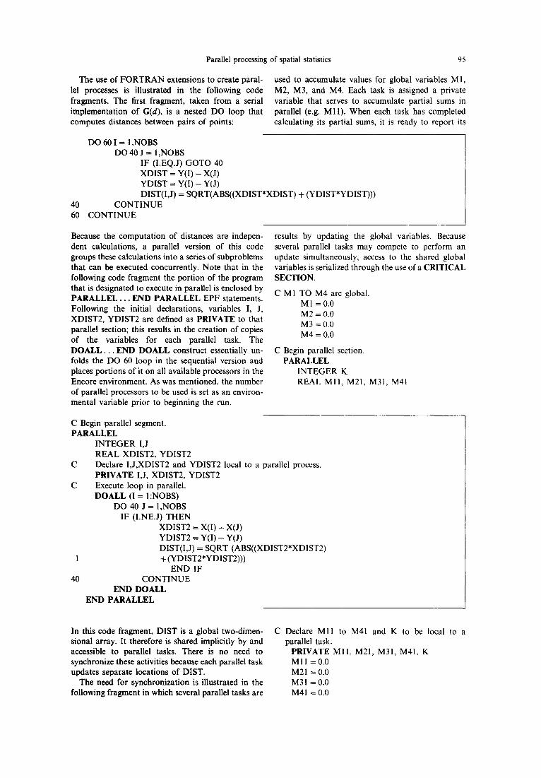
The use of FORTRAN extensions to create paral- lel processes is illustrated in the following code fragments. The first fragment, taken from a serial implementation of G(d), is a nested DO loop that computes distances between pairs of points:
used to accumulate values for global variables M1, M2, M3, and M4. Each task is assigned a private variable that serves to accumulate partial sums in parallel (e.g. M l l ) . When each task has completed calculating its partial sums, it is ready to report its
40 60
DO 601 = I,NOBS DO 40 J = I,NOBS
IF (I.EQ.J) GOTO 40 XDIST = Y(I) - X(J) YDIST = Y(I) - Y(J) DIST(I,J) = SQRT(ABS((XDIST*XDIST) + (YDIST*YDIST)))
CONTINUE CONTINUE
Because the computation of distances are indepen- dent calculations, a parallel version of this code groups these calculations into a series of subproblems that can be executed concurrently. Note that in the following code fragment the portion of the program that is designated to execute in parallel is enclosed by P A R A L L E L . . . END PARALLEL EPF statements. Following the initial declarations, variables I, J, XDIST2, YDIST2 are defined as PRIVATE to that parallel section; this results in the creation of copies of the variables for each parallel task. The D O A L L . . . END DOALL construct essentially un- folds the DO 60 loop in the sequential version and places portions of it on all available processors in the Encore environment. As was mentioned, the number of parallel processors to be used is set as an environ- mental variable prior to beginning the run.
results by updating the global variables. Because several parallel tasks may compete to perform an update simultaneously, access to the shared global variables is serialized through the use of a CRITICAL SECTION.
C M1 TO M4 are global. MI = 0.0 M2 = 0.0 M3 = 0.0 M4 = 0.0
C Begin parallel section. PARALLEL
INTEGER K REAL M l l , M21, M31, M41
C Begin parallel segment. PARALLEL
INTEGER I,J REAL XDIST2, YDIST2
C Declare I,J,XDIST2 and YDIST2 local to a parallel process. PRIVATE I,J, XDIST2, YDIST2
C Execute loop in parallel. DOALL (I = I:NOBS)
DO 40 J = 1,NOBS IF (I.NE.J) THEN
XDIST2 = X(I) - X(J) YDIST2 = Y(I) - Y(J) DIST(I,J) = SQRT (ABS((XDIST2*XDIST2)
1 + (YDIST2*YDIST2))) END IF
40 CONTINUE END DOALL
END PARALLEL
In this code fragment, DIST is a global two-dimen- sional array. It therefore is shared implicitly by and accessible to parallel tasks. There is no need to synchronize these activities because each parallel task updates separate locations of DIST.
The need for synchronization is illustrated in the following fragment in which several parallel tasks are
C Declare M i l to M41 and K to be local to a parallel task.
PRIVATE MII , M21, M31, M41, K MII ---0.0 M21 = 0.0 M31 = 0.0 M41 = 0.0
96 M. P ARMSTRONG, C. E. PAVLIK, and R. MARCIANO
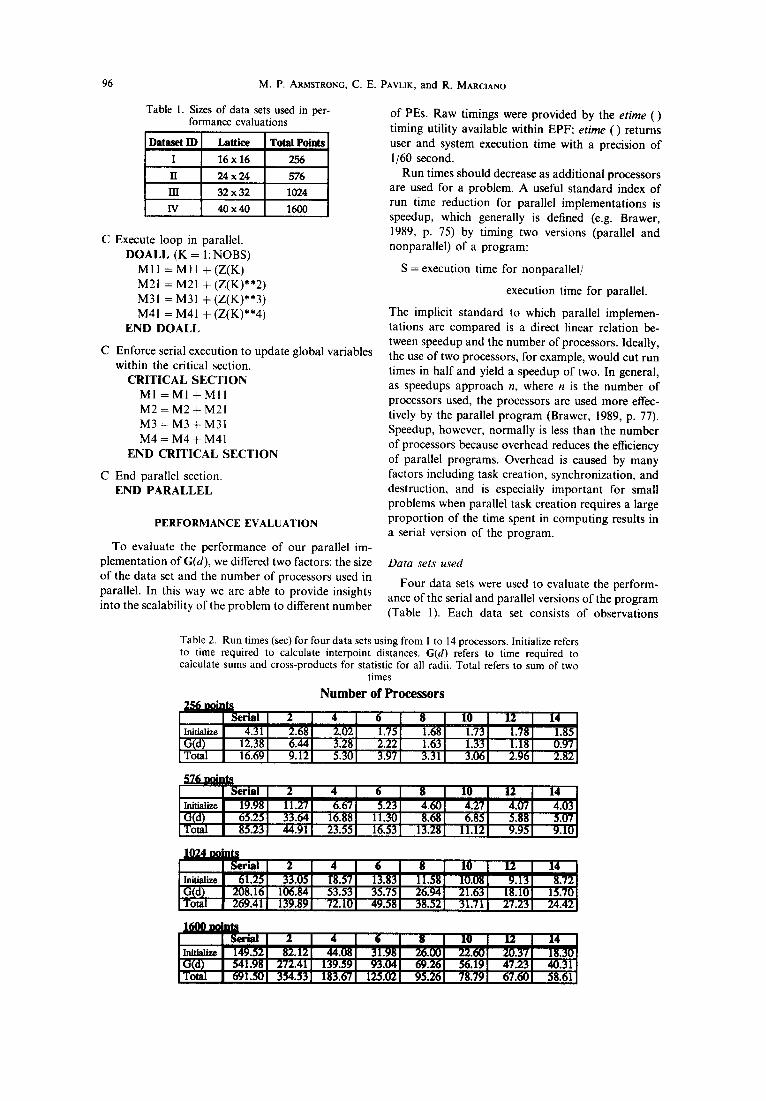
Table 1. Sizes of data sets used in per- formance evaluations
Dataset ID
I
IT
m
W
Lattice Total Points
16 x 16 256
24x24 576
32 x 32 1024
40 x 40 1600
C Execute loop in parallel. D O A L L (K -- 1: NOBS)
M I I = M I I ÷ ( Z ( K ) M21 = M21 + (Z(K)**2) M31 = M31 + (Z(K)**3) M41 = M41 + (Z(K)**4)
END D O A L L
C Enforce serial execution to update global variables within the critical section.
C R I T I C A L S E C T I O N MI = M l + M l l M2 = M2 + M21 M3 = M3 + M31 M4 = M4 + M41
END C R I T I C A L S E C T I O N
C End parallel section. END P A R A L L E L
PERFORMANCE EVALUATION
To evaluate the performance of our parallel im- plementation of G(d), we differed two factors: the size of the data set and the number of processors used in parallel. In this way we are able to provide insights into the scalability of the problem to different number
of PEs. Raw timings were provided by the etime ( ) timing utility available within EPF; etime ( ) returns user and system execution time with a precision of 1/60 second.
Run times should decrease as additional processors are used for a problem. A useful standard index of run time reduction for parallel implementations is speedup, which generally is defined (e.g. Brawer, 1989, p. 75) by timing two versions (parallel and nonparallel) of a program:
S = execution time for nonparallel/
execution time for parallel.
The implicit standard to which parallel implemen- tations are compared is a direct linear relation be- tween speedup and the number of processors. Ideally, the use of two processors, for example, would cut run times in half and yield a speedup of two. In general, as speedups approach n, where n is the number of processors used, the processors are used more effec- tively by the parallel program (Brawer, 1989, p. 77). Speedup, however, normally is less than the number of processors because overhead reduces the efficiency of parallel programs. Overhead is caused by many factors including task creation, synchronization, and destruction, and is especially important for small problems when parallel task creation requires a large proport ion of the time spent in computing results in a serial version of the program.
Data sets used
Four data sets were used to evaluate the perform- ance of the serial and parallel versions of the program (Table 1). Each data set consists of observations
Table 2. Run times (sec) for four data sets using from 1 to 14 processors. Initialize refers to time required to calculate interpoint distances. G(d) refers to time required to calculate sums and cross-products for statistic for all radii. Total refers to sum of two
times
Number of Processors 256 oints
Serial 2 4 6 8 10 12 14 Initialize 4.31 2.68 2.02 1.75 1.68 1.73 1.78 1.85 G(d) 12.38 6.44 3.28 2.22 1.63 1.33 1.18 0.97 Total 16.69 9.12 5.30 3.97 3.31 3.06 2.96 2.82
1600 noints
J m u . u , u u i i . ~
_ ' , i U U U i ~ l i i ~ m |:;YJ i km:~! i i L~:! i (lilt:! 'Jgl :kb.
i L ' r ~ m U U U U U U U
m
0 o M
t -
o E
n -
o I -
p,
Parallel processing of spatial statistics
7 0 0
6 0 0
5 0 0
4 0 0
3 0 0
2 0 0
1 0 0
0
2 5 6
I I I
5 7 6 1 0 2 4 1 6 0 0
Number of Observations
97
Figure 1. Effect of problem size on total computation time for serial version of program.
regularly spaced in a square with a side length of 32 units. The number of observations increases across data sets, so that larger data sets have more points per unit area. Larger data sets result in an increased com- putational burden for two reasons. First, as the number of observations increases, additional comparisons of distance values must be made for each G(d) statistic computed. Second, as the density of points increases, more observation sites fall within radius d so that additional xixfproducts must be calculated.
Timing results
The Encore system is a multiuser system and minor irregularities in timing on such systems may arise from a variety of causes. To eliminate effects that multiple users might have on overall system perform- ance, the timing results were obtained during low-use periods (e.g. 4 a.m.). Although we attempted to con-
trol access by scheduling our runs at low demand times and monitoring the system to ensure that usage was minimal, some logins may have occurred. In addition, processes for which we have no control could have been initiated by the operating system. Nevertheless, the results reported are indicative of what can be expected in performance improvements.
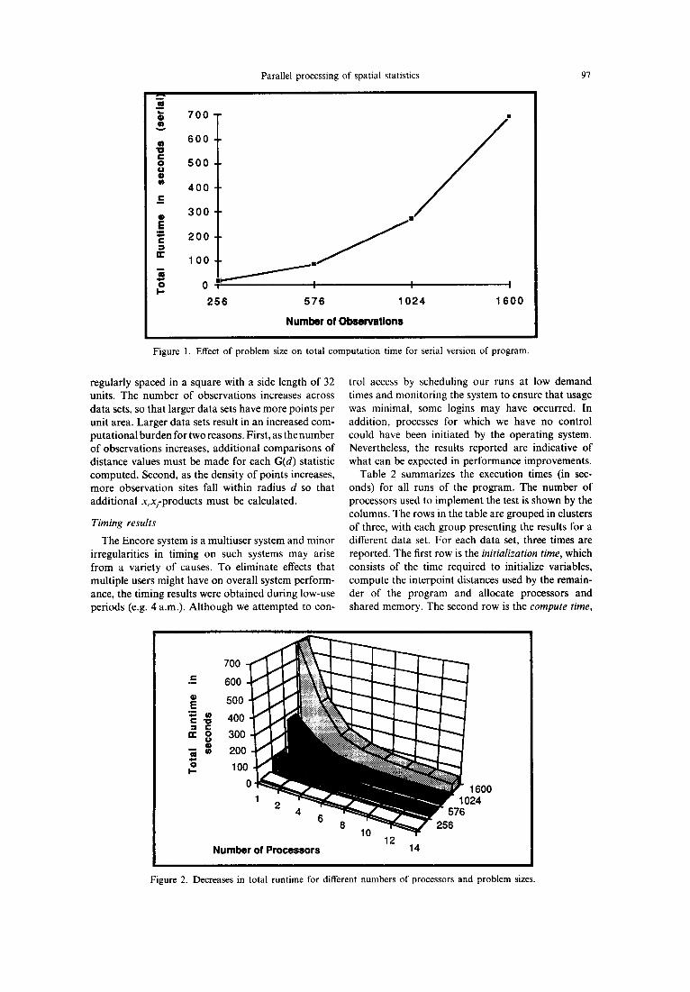
Table 2 summarizes the execution times (in sec- onds) for all runs of the program. The number of processors used to implement the test is shown by the columns. The rows in the table are grouped in clusters of three, with each group presenting the results for a different data set. For each data set, three times are reported. The first row is the initialization time, which consists of the time required to initialize variables, compute the interpoint distances used by the remain- der of the program and allocate processors and shared memory. The second row is the compute time,
700
600
500
400
30C
20C
lOq
0
E m .,.,
" "o = g
0 I -
II0
Number of Processors 14
1600 24
Figure 2. Decreases in total runtime for different numbers of processors and problem sizes.
98 M. P. ARMSTRONG, C. E. PAVLIK, and R. MARCIANO
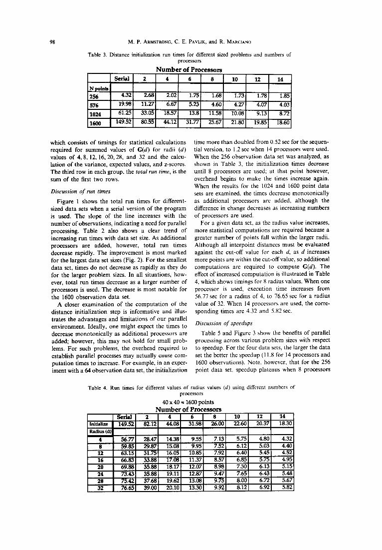
Table 3. Distance initialization run times for different sized problems and numbers of processors
N u m b e r o f Processors
Serial 2 4 6 8 10 12 14
N points 256 4.32
576 19.98
1024 61.25
1600 149.52
2.68 2.02 1.75 1.68 1.73 1.78 1.85
11.271 6.67 5.23 4.60 4.27 4.07 4.03
33.05 18.57 13.8 11.58 10.08 9.13 8.72
80.55 44.12 31.77 25.67 21.80 19.85 18.60
which consists of timings for statistical calculations required for summed values of G(d) for radii (d) values of 4, 8, 12, 16, 20, 28, and 32 and the calcu- lation of the variance, expected values, and z-scores. The third row in each group, the total run time, is the sum of the first two rows.
Discussion of run times
Figure 1 shows the total run times for different- sized data sets when a serial version of the program is used. The slope of the line increases with the number of observations, indicating a need for parallel processing. Table 2 also shows a clear trend of increasing run times with data set size. As additional processors are added, however, total run times decrease rapidly. The improvement is most marked for the largest data set sizes (Fig. 2). For the smallest data set, times do not decrease as rapidly as they do for the larger problem sizes. In all situations, how- ever, total run times decrease as a larger number of processors is used. The decrease is most notable for the 1600 observation data set.
A closer examination of the computation of the distance initialization step is informative and illus- trates the advantages and limitations of our parallel environment. Ideally, one might expect the times to decrease monotonically as additional processors are added; however, this may not hold for small prob- lems. For such problems, the overhead required to establish parallel processes may actually cause com- putation times to increase. For example, in an exper- iment with a 64 observation data set, the initialization
time more than doubled from 0.52 sec for the sequen- tial version, to 1.2 sec when 14 processors were used. When the 256 observation data set was analyzed, as shown in Table 3, the initialization times decrease until 8 processors are used; at that point however, overhead begins to make the times increase again. When the results for the 1024 and 1600 point data sets are examined, the times decrease monotonically as additional processors are added, although the difference in change decreases as increasing numbers of processors are used.
For a given data set, as the radius value increases, more statistical computations are required because a greater number of points fall within the larger radii. Although all interpoint distances must be evaluated against the cut-off value for each d, as d increases more points are within the cut-off value, so additional computations are required to compute G(d). The effect of increased computation is illustrated in Table 4, which shows timings for 8 radius values. When one processor is used, execution time increases from 56.77 sec for a radius of 4, to 76.65 sec for a radius value of 32. When 14 processors are used, the corre- sponding times are 4.32 and 5.82 sec.
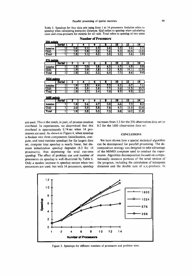
Discussion of speedups
Table 5 and Figure 3 show the benefits of parallel processing across various problem sizes with respect to speedup. For the four data sets, the larger the data set the better the speedup (11.8 for 14 processors and 1600 observations). Note, however, that for the 256 point data set, speedup plateaus when 8 processors
Table 4. Run times for different values of radius values (d) using different numbers of processors
40 X 40 = 1600 points N u m b e r of Processors
Serial 2 4 6 8 10 12 14 i Initialize 149.52 82.12 44.08 31.98 26.00 22.60 20.37 18.30 Radius (d)
4 56.77 28.47 14.38 9.55 7.13! 5.75 4.80 4.32 f
8 59.85 29.87 15.08 9.95 7.52 6.12 5.03 4.40 12 63.15 31.751 16.05 10.85 7.92 6.40 5.45 4.52 16 66.83 33.88 17.08 11.37 8.57 6.85 5.75 4.95 20 69.88 35.88 18.17 12.07 8.98 7.30 6.13 5.15 24 73.43 35.88 19.11 12.87 9.47 7.65 6.43 5.48 28 75.42 37.68 19.62 13.08 9.75 8.00 6.72 5.67 32 76.65 39.00 20.10 13.30 9.92 8.12 6.92 5.82
Parallel processing of spatial statistics
Table 5. Speedups for four data sets using from 1 to 14 processors. Initialize refers to speedup when calculating interpoint distances. G(d) refers to speedup when calculating sums and cross-products for statistic for all radii. Total refers to speedup of two times
Number of Processors
~ r l a l I 2 4 6 8 10 12 14 Initialize 1.6 2.1 2.5 2.6 2.5 2.4 2.3 G(d) 1 I 1.9 3.8 5.6 7.6 9.3 10.5 12.8 Total 1 1.8 3.1 4.2 5.0 5.5 5.6 5.9
99
m ~-~-~ m B L B B B K B B B L I B U BLg~B U BBglB ,-rr~trra ! M.. 'tb] M:! 9:] ,,~I -~1 ~l K , ~ l i | ~"1 ' ) ' ] ): ! _it. 'Jk| J i l l pI I • wrnnm i K'I ' ][~,I I~ p ] ;'~! Jl~ :Jr.-'] I"
m.-:.'z m -- I,m =mE
i r~r~a ! K'm ' Itl ,El lgl ,ill ,1hi ,11 ~ * ~ . l i | K'I ,!.] ~;! '-JlfJ '~1 |ll~l l - - t , ~ m I K'm ']bJ ~! ,.go] :It I ~ d ] g i ~ t l . I !
m. 'z m -- [, umm m
~ I , ~ m ! '-K*I '&'] )el ~;1 'M~ I ~ ~ q ~ t ,m m I i : m m m'I¢
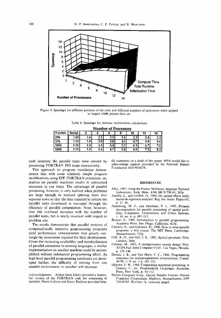
are used. This is the result, in part, of process creation overhead. In experiments, we determined that this overhead is approximately 0.74sec when 14 pro- cessors are used. As shown in Figure 4, when speedup is broken into three components (initialization, com- pute, and total runtime speedup) for the largest data set, compute time speedup is nearly linear, but dis- tance initialization speedup degrades (8.2 for 14 processors), thus depressing the total run-time speedup. The effect of problem size and number of processors on speedup is well-illustrated by Table 6. Only a modest increase in speedup occurs when two processors are used, but with 14 processors, speedup
increases from 2.3 for the 256 observation data set to 8.2 for the 1600 observation data set.
CONCLUSIONS
We have shown how a spatial statistical algorithm can be decomposed for parallel processing. The de- composition strategy was designed to take advantage of the MIMD computer used to conduct the exper- iments. Algorithm decomposition focused on compu- tationally intensive portions of the serial version of the program, including the calculation of interpoint distances and the double sum of xlx/-products. In
12
10
==. )° 4
0 , m ~ 1 6 0 0
[] 1 0 2 4
' 5 7 6
¢ 2 5 6
O ~
1 2 4 6 8 10 12 14
Number of Processors
Figure 3. Speedups for different numbers of processors and problem sizes.
100 M.P. ARMSTRONG, C. E. PAVLIK, and R. MARCIANO
12
10
8 -
6- 4. 2 - 0
1
{:1.
g=. ¢./)
Number of Processors 1;," 14
3ompute Time :al Runtime
zation Time
Figure 4. Speedups for different portions of the code and different numbers of processors when applied to largest (1600 points) data set.
Table 6. Speedups for distance initialization calculations
N u m b e r o f P r o c e s s o r s N points Serial 2 4
256 1.00 1.6 2.1] 576 1.00 1.8 3.0 1024 1.00 1.9 3.3 1600 1.00 1.9 3.4
6 8 10 12 14 2.5 2.6 2.5 2.4 2.3 3.8 4.3 4.7 4.9 5.0 4.4 5.3 6.1 6.7 7.0 4.7 5.8 6.9 7.5 8.2
each situation the parallel tasks were created by processing F O R T R A N DO loops concurrently.
This approach to program translation demon- strates that with some relatively simple program modifications using EPF F O R T R A N extensions, ex- ecution on parallel machines results in substantial decreases in run times. The advantage of parallel processing, however, is only realized when problems are large enough to warrant splitting them into separate tasks so that the time required to initiate the parallel tasks (overhead) is recouped through the efficiency of parallel computation. Note, however, that this overhead increases with the number of parallel tasks, but is nearly invariant with respect to problem size.
The results demonstrate that parallel versions of computationally intensive geoprocessing programs yield performance enhancements that greatly out- weigh the investment required for their development. Given the increasing availability and standardization of parallel extensions to existing languages, a similar implementation on another machine could be accom- plished without substantial programming effort. As high-level parallel programming constructs are devel- oped further, the difficulty of moving from one parallel environment to another will decrease.
Acknowledgments--Arthur Getis kindly provided a sequen- tial version of the FORTRAN code for computing G statistics. Panos Lolonis and Gerry Rushton provided help-
ful comments on a draft of this paper. MPA would like to acknowledge support provided by the National Science Foundation SES-9024278.
REFERENCES
ANL, 1987, Using the Encore Multimax: Argonne National Laboratory, Tech. Mem. ANL/MCS-TM-65, 263p.
Anselin, L., and Griffith, D., 1988, Do spatial effects really matter in regresson analysis?: Reg. Sci. Assoc. Papers 65, p. ll 34.
Armstrong, M. P., and Densham, P. J., 1992, Domain decomposition for parallel processing of spatial prob- lems: Computers, Environment and Urban Systems, v. 16, no. 6, p. 497 513.
Brawer, S., 1989, Introduction to parallel programming: Academic Press, San Diego, California, 423p.
Carriero, N., and Gelernter, D., 1990, How to write parallel programs: a first course: The MIT Press, Cambridge, Massachussets, 232p.
Cliff, m. D., and Ord, J. K., 1981, Spatial processes: Pion, London, 266p.
Conway, M., 1963, A multiprocessor system design: Proc. AFIPS Fall Joint Computer Conf., Las Vegas, Nevada, p. 139--146.
Dennis, J. B., and Van Horn, E. C., 1966, Programming semantics for multiprogrammed computations: Comm. ACM, v. 9, no. 3 p. 143-155.
Dijkstra, E. W., 1968, Cooperating sequential processing, in Genuys, F., ed., Programming Languages: Academic Press, New York, p. 43-112.
Encore Computer Corp., Encore Parallel Fortran: Encore Computer Corporation, Malboro, Massachusetts, EPF 724-06785, Revision A, variously paged.
Parallel processing of spatial statistics 101
Flynn, M. J., 1966, Very high speed computing systems: Proc. IEEE, v. 54, no. 12, p. 1901-1909.
Getis, A., and Ord, J. K., 1992, The analysis of spatial association by use of distance statistics: Geographical Analysis, v. 24, no. 3, p. 189-206.
Grit~th, D., 1990, Supercomputing and spatial statistics: a reconnaissance: The Professional Geographer, v. 42, no. 4, p. 481-492.
Hwang, K., and DeGroot, D., 1989, Parallel programming environment and software support, in Hwang, K., and Degroot, D., eds., Parallel processing for supercomput- ers and artificial intelligence: McGraw-Hill Book Co., New York, p. 369-408.
Lilja, D. J., 1991, Architectural alternatives for exploiting parallelism: IEEE Computer Society Press, Los Alami- tos, California, 447p.
MacDougall, E. B., 1984, Surface mapping with weighted averages in a microcomputer, in Spatial algorithms for processing land data with a microcomputer: Lincoln Inst. Mon. 84-2, Cambridge, Massachusetts, p. 125-152.
Mills, K., Fox, G., and Heimbach, R., 1992, Implementing an intervisibility analysis model on a parallel computing system: Computers & Geosciences, v. 18, no. 8, p. 1047-1054.
Myers, W., 1993, Supercomputing 92 reaches down to the workstation: IEEE Computer, v. 26, no. 1, p. 113-117.
Oliver, M., Webster, R., and Gerrard, J., 1989a, Geostatis- tics in physical geography. Part I: theory: Trans. Inst. British Geographers, v. 14, no. 3, p. 259-269.
Oliver, M., Webster, R., and Gerrard, J., 1989b, Geostatis- tics in physical geography. Part II: applications: Trans. Inst. British Geographers. v. 14, no. 3, p. 270-286.
Openshaw, S., Cross, A., and Charlton, M., 1990, Building a prototype Geographical Correlates Exploration Machine: Intern. Jour. Geographical Information Systems, v. 4, no. 3, p. 297-312.
Pancake, C. M., 1991, Software support for parallel com- puting: where are we headed?: Comm. Assoc. Comput- ing Machinery, v. 34, no. 11, p. 52~)4.
Sandhu, J. S., and Marble, D. F., 1988, An investigation into the utility of the Cray X-MP supercomputer for handling spatial data: Proc. Third Intern. Syrup. Spatial Data Handling, IGU Commission on GIS, Columbia, South Carolina, p. 253-267.
Shen, Z., Li, Z., and Yew, P-C., 1990, An empirical study of Fortran programs for parallelizing compilers: IEEE Trans. Parallel and Distributed Systems, v. 1, no. 3, p. 356-364.
A P P E N D I X
EPF Version of G-stat
C
PROGRAM GSTAT REAL X(2500),Y(2500),Z(2500),DIST(2500,2500),W(2500) REAL ZSUM,STEP,XDIST,YDIST, ZS,M1 ,M2,M3,M4 REAL G,VARG,ZSCORE,MAX, INC,NOBS REAL S1,S2,B0,B1,B2,B3,B4,EG,EG2 REAL BOA,BOB,BOC,BIA, BIB,BIC,B2A, B2B, B2C,B3A, B3B, B3C REAL EAA, EA,MM1,MM2,MM3,MM4,EG2A,R INTEGER A,I,J,K,WT,WA,WB CHARACTER * 40 INNAME,OUTNAM DATA ZSUM,STEP,XDIST,YDIST, ZS,M1,M2,M3,M4/9*0.0/ DATA G,VARG,ZSCORE,MAX,INC,NOBS/6*0.0/ DATA S1,S2,B0,B1,B2,B3,B4,EG,EG2/9*0.0/ DATA BOA,BOB,BOC,BIA, BIB,BIC, B2A, B2B, B2C,B3A, B3B,B3C/12"0.0/ DATA EAA,EA,MM1,MM2,MM3,MM4,EGZA,R/8*0.0/ DATA A,I,J,K,WT,WA,WB/7*0/ real t_start, Lend, tmp(2), t l , t2
DO 10 A=1,20000 READ (1,*,END=20) X(A),Y(A),Z(A)
10 CONTINUE
WRITE (*,*) 'INPUT FILE NAME?' WRITE (*,*) READ (*,I) INNAME WRITE (*,*) 'OU'I~UT FILE NAME?' WRITE (*,*) READ ('1) OUTNAM 1 FORMAT (A) OPEN (1,FILE=IN'NAME,STATUS='OLD') OPEN (2,FILE--OUTNAM,STATUS='OLD') WRITE (~,*) 'MAXIMUM SEARCH RADIUS?' WRITE (**) READ (*,*) MAX WRrFE (**) 'NUMBER OF INCREMENTS?' WRITE (*,*) READ (~,*) INC WRITE (2,*) ' STEP G EG G-EG',
1 'VARG ZSCORE NOBS' WRITE (2,*) '
102 M.P . ARMSTRONG, C. E. PAVLIK, and R. MARCIANO
t_start = et ime( tmp) 20 NOBS=A-1
SI=0.0 MI=0.0 M2=0.0 M3=0.0 M4=0.0 PARALLEL
INTEGER K REAL M l l , M21, M31, M41 PRIVATE M l l , M21, M31, M41, K
M l l = 0.0 M21 = 0.0 M31 = 0.0 M41 = 0.0
DOALL (K=I:NOBS) M l l = M l l + Z(K) M21 = M21 + (Z(K) ** 2) M31 = M31 + (Z(K) ** 3) M41 = M41 + (Z(K) ** 4)
E N D DOALL
C R m C A L SECTION M1 = M1 + M l l M2 = M 2 + M21 M3 = M3 +M31 M4 = M 4 + M41
END CRITICAL SECTION E N D PARALLEL
MMI=M4/(M2**2) MM2=(MI**2) /M2 M M 3 = ( M I * M 3 ) / ( M 2 " 2 ) MM4=(MI**4) / (M2"2)
PARALLEL INTEGER I, J REAL XDIST2, YDIS3R PRIVATE I, J, XDIST2, YDIST2
1
40
DOALL (I=l :NOBS) DO 40 J=I,NOBS
IF (I .NE. J) THEN XDIST2 = X(I) - X(J) YDIST2 = Y(I)- Y(J) DIST(I,J) = SQRT (ABS ((XDIST2 * XDIST2)
+ (YDIST2 * YDIST2))) END IF
CONTINUE E N D DOALL
E N D PARALLEL t_end = et ime( tmp) t l = ( t e n d - t_start) pr in t *,' + Init ial ization Time = ', t l p r in t * , "
STEP=O.O 70 STEP=STEP+(MAX/INC)
pr in t *, ' m STEP = ', STEP t_start = e t ime( tmp)
ZSUM=0.0

Parallel processing of spatial statistics 103
ZS---0.0 WT=0.0 WA=0.0 P A R A L L E L
INTEGER WT1, I, J, W A 2 REAL ZSUM1, 7-_51 P R I V A T E ZSUM1, ZS1, WT1, I, J, W A 2
WT1 = 0 ZS1 -- 0.0 ZSUM1 = 0.0
D O A L L (I=I:NOBS) W A 2 = 0.0 DO 30 J=I ,NOBS
IF (I .NE. J) T H E N ZSUM1 = ZSUM1 + (Z(I) * z(J)) IF (DIST(I,J) .LE. STEP) T H E N
ZS1 = ZS1 + (Z(I) * Z(J)) WT1 = WT1 + 1 W A 2 = W A 2 + 1 W(I) = W A 2
E N D IF E N D IF
30 C O N T I N U E E N D D O A L L
C R I T I C A L S E C T I O N W T = W T + WT1 ZS = ZS + ZS1 Z S U M = Z S U M + ZSUM1
E N D C R I T I C A L S E C T I O N E N D P A R A L L E L
R=(WT*M2)/ (NOBS*(MI*M1-M2)) EG=WT/((NOBS)*(NOBS-1)) G=ZS/ZSUIVl
W'I2=WT*"2 EAA=WT2*(NOBS-3)*(NOBS-2)*(NOBS-1 ) E A = N O B S / E A A
WB=0 $2=0.0 P A R A L L E L
INTEGER I REAL S21,WB1 P R I V A T E $21, WB1, I
WB1 = 0.0 $21 = 0.0
D O A L L (I=I:NOBS) WBI=WB1 +W(I) $21 = $21 + ((2 * W(I)) ** 2)
E N D D O A L L
C R I T I C A L S E C T I O N W B = W B + WB1 $2 = $2 + $ 2 1
E N D C R I T I C A L S E C T I O N E N D P A R A L L E L
$ 1 = ( 4 " W B ) / 2 N2=NOBS**2
BOA=N2-(3"NOBS)+3
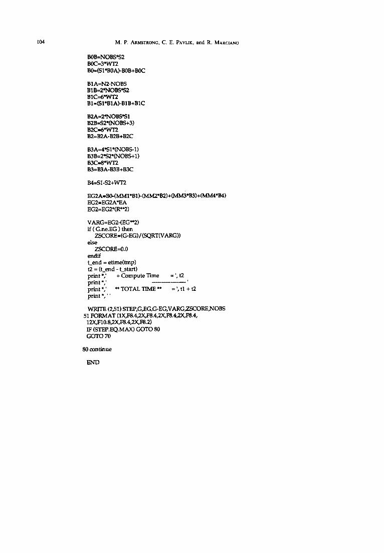
104 M.P. ARMSTRONG, C. E. PAVLIK, and R. MARCIANO
BOB=NOBS~S2 BOC=3*WT2 B0=(SI*BOA)-BOB+BOC
B1A=N2-NOBS BIB=2*NOBSIS2 BIC=6*WT2 BI=(SI*BIA)-BIB+BIC
B2A=2*NOBSI"S1 B2B=S2*(NOBS+3) B2C=6*WT2 B2=B2A-B2B+B2C
B3A=4*SI*(NOBS-1) B3B=2*S2*(NOBS+I) B3C--8*WT2 B3=B3A-B3B+B3C
B4=$1 -S2+WT2
EG2A-~B0-(MMI*B1)-(MM2*B2)+(MM3*B3)+(MM4*B4) EG2=EG2A*EA EG2=EG2*(R**2)
VARG=EG2-(EG*~) if ( G.ne.EG ) then
ZSCORE=(G-EG) / (SQRT(VARG)) else
ZSCORE=0.0 endif Lend = etime(tmp) t2 = ( t e n d - t s ta r t ) print *,' + Compute Time print *,' print *,' ** TOTAL TIME ** print * ,"
= I e t 2
= ' , t l +t2
WRITE (2,51) STEP,G,EG,G-EG,VARG,ZSCORE,NOBS 51 FORMAT (1X,F8.4,2X,F8.4,2X,FS.4,2X,F8.4,
12X,F10.8,2X,F8.4,2X, F8.2) IF (STEP.EQ.MAX) GOTO 80 GOTO 70
80 continue
END